efficient identification of improving moves in a ball for pseudo-boolean problems
TRANSCRIPT

1 / 28 GECCO 2014, Vancouver, Canada, July 14
Introduction Background Contribution Experiments Conclusions & Future Work
Efficient Identification of Improving Moves in a Ball for Pseudo-Boolean Problems
Francisco Chicano, Darrell Whitley, Andrew M. Sutton
2 / 28 GECCO 2014, Vancouver, Canada, July 14
Introduction Background Contribution Experiments Conclusions & Future Work
r = 1 n
r = 2�n2
�
r = 3�n3
�
r
�nr
�
BallPr
i=1
�ni
�
S1(x) = f(x� 1)� f(x)
Sv(x) = f(x� v)� f(x) =mX
l=1
(f (l)(x� v)� f
(l)(x)) =mX
l=1
S
(l)(x)
S4(x) = f(x� 4)� f(x)
S1,4(x) = f(x� 1, 4)� f(x)
S1,4(x) = S1(x) + S4(x)
S1(x) = f
(1)(x� 1)� f
(1)(x)
S2(x) = f
(1)(x� 2)� f
(1)(x) + f
(2)(x� 2)� f
(2)(x) + f
(3)(x� 2)� f
(3)(x)
S1,2(x) = f
(1)(x�1, 2)�f
(1)(x)+f
(2)(x�1, 2)�f
(2)(x)+f
(3)(x�1, 2)�f
(3)(x)
S1,2(x) 6= S1(x) + S2(x)
f(x) =NX
l=1
f
(l)(x)
1
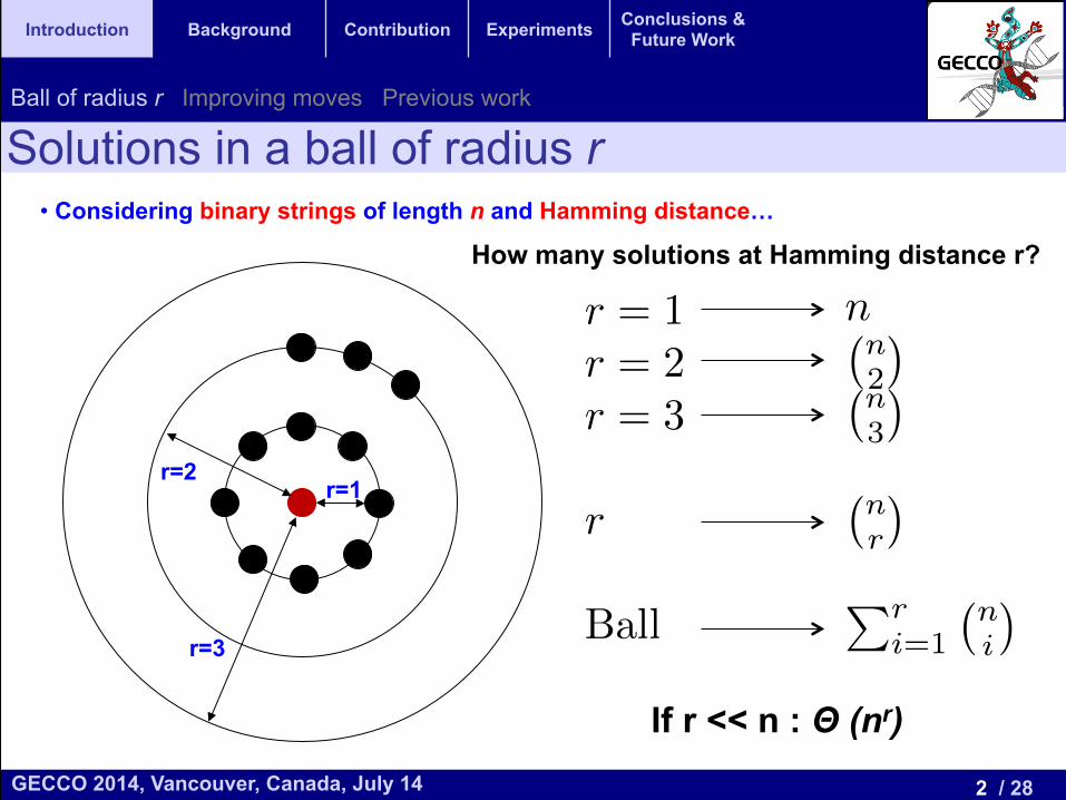
• Considering binary strings of length n and Hamming distance…
Solutions in a ball of radius r
r=1 r=2
r=3
Ball of radius r Improving moves Previous work
How many solutions at Hamming distance r?
If r << n : Θ (nr)
3 / 28 GECCO 2014, Vancouver, Canada, July 14
Introduction Background Contribution Experiments Conclusions & Future Work
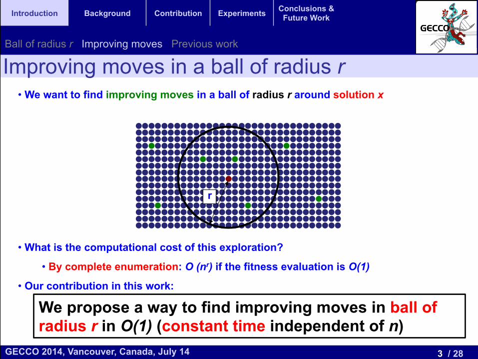
• We want to find improving moves in a ball of radius r around solution x
• What is the computational cost of this exploration?
• By complete enumeration: O (nr) if the fitness evaluation is O(1)
• Our contribution in this work:
Improving moves in a ball of radius r
r
We propose a way to find improving moves in ball of radius r in O(1) (constant time independent of n)
Ball of radius r Improving moves Previous work
4 / 28 GECCO 2014, Vancouver, Canada, July 14
Introduction Background Contribution Experiments Conclusions & Future Work
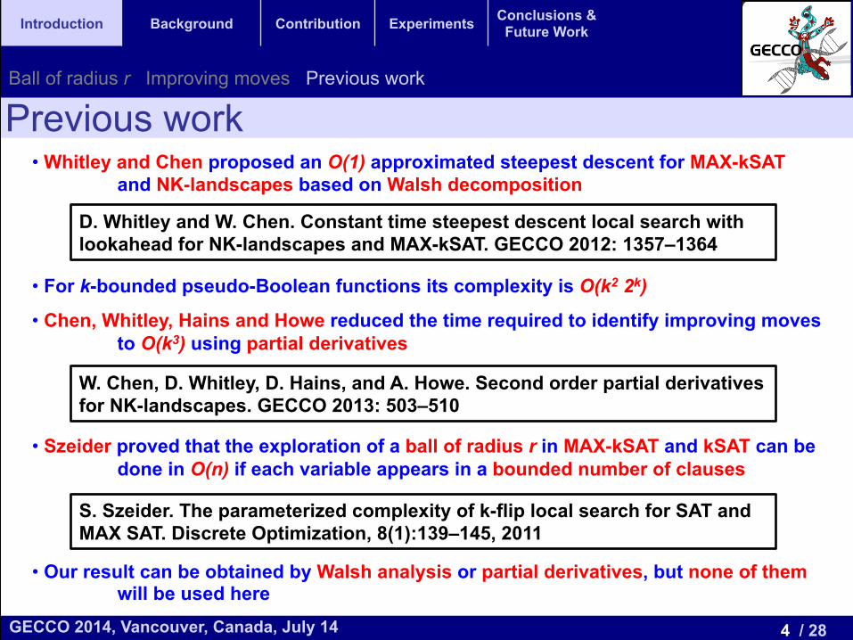
• Whitley and Chen proposed an O(1) approximated steepest descent for MAX-kSAT and NK-landscapes based on Walsh decomposition
• For k-bounded pseudo-Boolean functions its complexity is O(k2 2k)
• Chen, Whitley, Hains and Howe reduced the time required to identify improving moves to O(k3) using partial derivatives
• Szeider proved that the exploration of a ball of radius r in MAX-kSAT and kSAT can be done in O(n) if each variable appears in a bounded number of clauses
• Our result can be obtained by Walsh analysis or partial derivatives, but none of them will be used here
Previous work Ball of radius r Improving moves Previous work
D. Whitley and W. Chen. Constant time steepest descent local search with lookahead for NK-landscapes and MAX-kSAT. GECCO 2012: 1357–1364
W. Chen, D. Whitley, D. Hains, and A. Howe. Second order partial derivatives for NK-landscapes. GECCO 2013: 503–510
S. Szeider. The parameterized complexity of k-flip local search for SAT and MAX SAT. Discrete Optimization, 8(1):139–145, 2011
5 / 28 GECCO 2014, Vancouver, Canada, July 14
Introduction Background Contribution Experiments Conclusions & Future Work
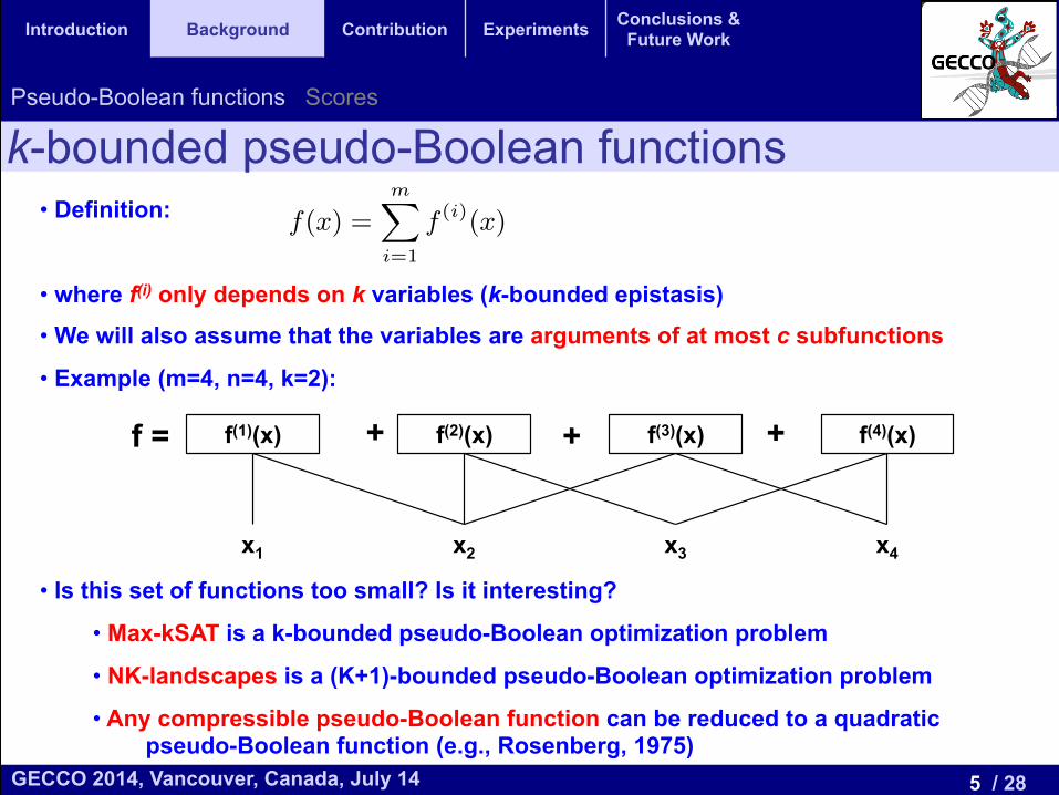
• Definition:
• where f(i) only depends on k variables (k-bounded epistasis)
• We will also assume that the variables are arguments of at most c subfunctions
• Example (m=4, n=4, k=2):
• Is this set of functions too small? Is it interesting?
• Max-kSAT is a k-bounded pseudo-Boolean optimization problem
• NK-landscapes is a (K+1)-bounded pseudo-Boolean optimization problem
• Any compressible pseudo-Boolean function can be reduced to a quadratic pseudo-Boolean function (e.g., Rosenberg, 1975)
k-bounded pseudo-Boolean functions Pseudo-Boolean functions Scores
derivative, they reduce the time needed to identify improv-ing moves from O(k22k) to O(k3). In addition, the newapproach avoids the use of the Walsh transform, making theapproach conceptually simpler.
In this paper, we generalize this result to present a localsearch algorithm that can look r moves ahead and iden-tify all improving moves. This means that moves are beingidentified in a neighborhood containing all solutions that liewithin a Hamming ball of radius r around the current so-lution. We assume that r = O(1). If r ⌧ n, the numberof solutions in such a neighborhood is ⇥(nr). New improv-ing moves located up to r moves away can be identified inconstant time. The memory required by our approach isO(n). To achieve O(1) time per move, the number of sub-functions in which any variable appears must be bounded bysome constant c. We then prove that the resulting algorithmrequires O((3kc)rn) space to track potential moves.
In order to evaluate our approach we perform an experi-mental study based on NKq-landscapes. The results revealnot only that the time required by the next ascent is inde-pendent of n, but also that increasing r we obtain a signifi-cant gain in the quality of the solutions found.
The rest of the paper is organized as follows. In the nextsection we introduce the pseudo-Boolean optimization prob-lems. Section 3 defines the“Scores”of a solution and providean algorithm to e�ciently update them during a local searchalgorithm. We propose in Section 4 a next ascent hill climberwith the ability to identify improving moves in a ball of ra-dius r in constant time. Section 5 empirically analyzes thishill climber using NKq-landscapes instances and Section 6outlines some conclusions and future work.
2. PSEUDO-BOOLEAN OPTIMIZATIONOur method for identifying improving moves in the radius
r Hamming ball can be applied to all k-bounded pseudo-Boolean Optimization problems. This makes our methodquite general: every compressible pseudo-Boolean Optimiza-tion problem can be transformed into a quadratic pseudo-Boolean Optimization problem with k = 2.
The family of k-bounded pseudo-Boolean Optimizationproblems have also been described as an embedded landscape.An embedded landscape [3] with bounded epistasis k is de-fined as a function f(x) that can be written as the sumof m subfunctions, each one depending at most on k inputvariables. That is:
f(x) =mX
i=1
f (i)(x), (1)
where the subfunctions f (i) depend only on k componentsof x. Embedded Landscapes generalize NK-landscapes andthe MAX-kSAT problem. We will consider in this paper thatthe number of subfunctions is linear in n, that is m 2 O(n).For NK-landscapes m = n and is a common assumption inMAX-kSAT that m 2 O(n).
3. SCORES IN THE HAMMING BALLFor v, x 2 Bn, and a pseudo-Boolean function f : Bn ! R,
we denote the Score of x with respect to move v as Sv(x),defined as follows:1
Sv(x) = f(x� v)� f(x), (2)1We omit the function f in Sv(x) to simplify the notation.
where � denotes the exclusive OR bitwise operation. TheScore Sv(x) is the change in the objective function when wemove from solution x to solution x� v, that is obtained byflipping in x all the bits that are 1 in v.All possible Scores for strings v with |v| r must be
stored as a vector. The Score vector is updated as localsearch moves from one solution to another. This makes itpossible to know where the improving moves are in a ball ofradius r around the current solution. For next ascent, all ofthe improving moves can be bu↵ered. An approximate formof steepest ascent local search can be implemented usingmultiple bu↵ers [9].If we naively use equation (2) to explicitly update this
Score vector, we will have to evaluate allPr
i=0
�ni
�neigh-
bors in the Hamming ball. Instead, if the objective functionsatisfies some requirements described below, we can designan e�cient next ascent hill climber for the radius r neigh-borhood that only stores a linear number of Score values andrequires a constant time to update them. We next explainthe theoretical foundations of this next ascent hill climber.The first requirement for the objective function is that it
must be written such that each subfunction depends only onk Boolean variables of x (k-bounded epistasis). In this case,we can write the scoring function Sv(x) as an embeddedlandscape:
Sv(x) =mX
l=1
⇣f (l)(x� v)� f (l)(x)
⌘=
mX
l=1
S(l)v (x), (3)
where we use S(l)v to represent the scoring functions of the
subfunctions f (l). Let us define wl 2 Bn as the binary stringsuch that the i-th element of wl is 1 if and only if f (l) dependson variable xi. The vector wl can be considered as a maskthat characterizes the variables that a↵ect f (l). Since f (l)
has bounded epistasis k, the number of ones in wl, denotedwith |wl|, is at most k. By the definition of wl, the nextequalities immediately follow.
f (l)(x� v) = f (l)(x) for all v 2 Bn with v ^ wl = 0, (4)
S(l)v (x) =
⇢0 if wl ^ v = 0,
S(l)v^wl
(x) otherwise.(5)
Equation (5) claims that if none of the variables thatchange in the move characterized by v is an argument off (l) the Score of this subfunction is zero, since the value ofthis subfunction will not change from f (l)(x) to f (l)(x� v).On the other hand, if f (l) depends on variables that change,we only need to consider for the evaluation of S
(l)v (x) the
changed variables that a↵ect f (l). These variables are char-acterized by the mask vector v ^ wl. With the help of (5)we can write (3) as:
Sv(x) =mX
l=1wl^v 6=0
S(l)v^wl
(x), (6)
3.1 Scores DecompositionThe Score values in a ball of radius r give more informa-
tion than just the change in the objective function for movesin that ball. Let us illustrate this idea with the moves in theballs of radius r = 1 and r = 2. Let us assume that xi andxj are two variables that do not appear together as argu-ments of any subfunction f (l). Then, the Score of the move
f = + + + f(1)(x) f(2)(x) f(3)(x) f(4)(x)
x1 x2 x3 x4
6 / 28 GECCO 2014, Vancouver, Canada, July 14
Introduction Background Contribution Experiments Conclusions & Future Work
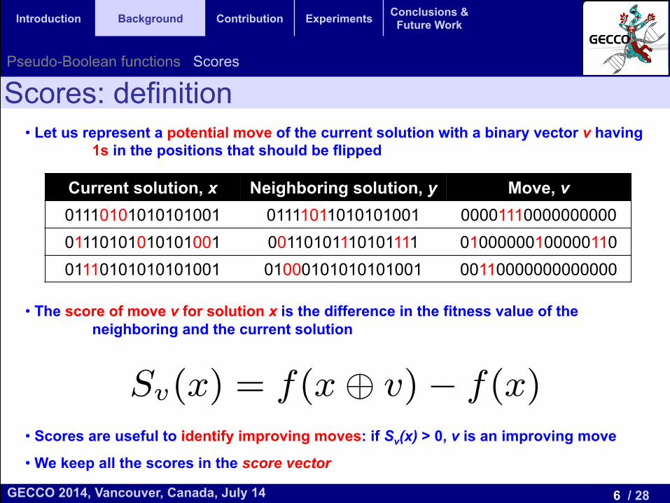
• Let us represent a potential move of the current solution with a binary vector v having 1s in the positions that should be flipped
• The score of move v for solution x is the difference in the fitness value of the neighboring and the current solution
• Scores are useful to identify improving moves: if Sv(x) > 0, v is an improving move
• We keep all the scores in the score vector
Scores: definition
Current solution, x Neighboring solution, y Move, v 01110101010101001 01111011010101001 00001110000000000 01110101010101001 00110101110101111 01000000100000110 01110101010101001 01000101010101001 00110000000000000
derivative, they reduce the time needed to identify improv-ing moves from O(k22k) to O(k3). In addition, the newapproach avoids the use of the Walsh transform, making theapproach conceptually simpler.
In this paper, we generalize this result to present a localsearch algorithm that can look r moves ahead and iden-tify all improving moves. This means that moves are beingidentified in a neighborhood containing all solutions that liewithin a Hamming ball of radius r around the current so-lution. We assume that r = O(1). If r ⌧ n, the numberof solutions in such a neighborhood is ⇥(nr). New improv-ing moves located up to r moves away can be identified inconstant time. The memory required by our approach isO(n). To achieve O(1) time per move, the number of sub-functions in which any variable appears must be bounded bysome constant c. We then prove that the resulting algorithmrequires O((3kc)rn) space to track potential moves.
In order to evaluate our approach we perform an experi-mental study based on NKq-landscapes. The results revealnot only that the time required by the next ascent is inde-pendent of n, but also that increasing r we obtain a signifi-cant gain in the quality of the solutions found.
The rest of the paper is organized as follows. In the nextsection we introduce the pseudo-Boolean optimization prob-lems. Section 3 defines the“Scores”of a solution and providean algorithm to e�ciently update them during a local searchalgorithm. We propose in Section 4 a next ascent hill climberwith the ability to identify improving moves in a ball of ra-dius r in constant time. Section 5 empirically analyzes thishill climber using NKq-landscapes instances and Section 6outlines some conclusions and future work.
2. PSEUDO-BOOLEAN OPTIMIZATIONOur method for identifying improving moves in the radius
r Hamming ball can be applied to all k-bounded pseudo-Boolean Optimization problems. This makes our methodquite general: every compressible pseudo-Boolean Optimiza-tion problem can be transformed into a quadratic pseudo-Boolean Optimization problem with k = 2.
The family of k-bounded pseudo-Boolean Optimizationproblems have also been described as an embedded landscape.An embedded landscape [3] with bounded epistasis k is de-fined as a function f(x) that can be written as the sumof m subfunctions, each one depending at most on k inputvariables. That is:
f(x) =mX
i=1
f (i)(x), (1)
where the subfunctions f (i) depend only on k componentsof x. Embedded Landscapes generalize NK-landscapes andthe MAX-kSAT problem. We will consider in this paper thatthe number of subfunctions is linear in n, that is m 2 O(n).For NK-landscapes m = n and is a common assumption inMAX-kSAT that m 2 O(n).
3. SCORES IN THE HAMMING BALLFor v, x 2 Bn, and a pseudo-Boolean function f : Bn ! R,
we denote the Score of x with respect to move v as Sv(x),defined as follows:1
Sv(x) = f(x� v)� f(x), (2)1We omit the function f in Sv(x) to simplify the notation.
where � denotes the exclusive OR bitwise operation. TheScore Sv(x) is the change in the objective function when wemove from solution x to solution x� v, that is obtained byflipping in x all the bits that are 1 in v.All possible Scores for strings v with |v| r must be
stored as a vector. The Score vector is updated as localsearch moves from one solution to another. This makes itpossible to know where the improving moves are in a ball ofradius r around the current solution. For next ascent, all ofthe improving moves can be bu↵ered. An approximate formof steepest ascent local search can be implemented usingmultiple bu↵ers [9].If we naively use equation (2) to explicitly update this
Score vector, we will have to evaluate allPr
i=0
�ni
�neigh-
bors in the Hamming ball. Instead, if the objective functionsatisfies some requirements described below, we can designan e�cient next ascent hill climber for the radius r neigh-borhood that only stores a linear number of Score values andrequires a constant time to update them. We next explainthe theoretical foundations of this next ascent hill climber.The first requirement for the objective function is that it
must be written such that each subfunction depends only onk Boolean variables of x (k-bounded epistasis). In this case,we can write the scoring function Sv(x) as an embeddedlandscape:
Sv(x) =mX
l=1
⇣f (l)(x� v)� f (l)(x)
⌘=
mX
l=1
S(l)v (x), (3)
where we use S(l)v to represent the scoring functions of the
subfunctions f (l). Let us define wl 2 Bn as the binary stringsuch that the i-th element of wl is 1 if and only if f (l) dependson variable xi. The vector wl can be considered as a maskthat characterizes the variables that a↵ect f (l). Since f (l)
has bounded epistasis k, the number of ones in wl, denotedwith |wl|, is at most k. By the definition of wl, the nextequalities immediately follow.
f (l)(x� v) = f (l)(x) for all v 2 Bn with v ^ wl = 0, (4)
S(l)v (x) =
⇢0 if wl ^ v = 0,
S(l)v^wl
(x) otherwise.(5)
Equation (5) claims that if none of the variables thatchange in the move characterized by v is an argument off (l) the Score of this subfunction is zero, since the value ofthis subfunction will not change from f (l)(x) to f (l)(x� v).On the other hand, if f (l) depends on variables that change,we only need to consider for the evaluation of S
(l)v (x) the
changed variables that a↵ect f (l). These variables are char-acterized by the mask vector v ^ wl. With the help of (5)we can write (3) as:
Sv(x) =mX
l=1wl^v 6=0
S(l)v^wl
(x), (6)
3.1 Scores DecompositionThe Score values in a ball of radius r give more informa-
tion than just the change in the objective function for movesin that ball. Let us illustrate this idea with the moves in theballs of radius r = 1 and r = 2. Let us assume that xi andxj are two variables that do not appear together as argu-ments of any subfunction f (l). Then, the Score of the move
Pseudo-Boolean functions Scores

7 / 28 GECCO 2014, Vancouver, Canada, July 14
Introduction Background Contribution Experiments Conclusions & Future Work
• The key idea of our proposal is to compute the scores from scratch once at the beginning and update their values as the solution moves (less expensive)
Scores update Main idea Decomposition of scores Constant time update
r
Selected improving move
Update the score vector

8 / 28 GECCO 2014, Vancouver, Canada, July 14
Introduction Background Contribution Experiments Conclusions & Future Work
• The key idea of our proposal is to compute the scores from scratch once at the beginning and update their values as the solution moves (less expensive)
• How can we do it less expensive?
• We have still O(nr) scores to update!
• … thanks to two key facts:
• We don’t need all the O(nr) scores to know if there is an improving move
• From the ones we need, we only have to update a constant number of them and we can do each update in constant time
Key facts for efficient scores update
r
Main idea Decomposition of scores Constant time update
9 / 28 GECCO 2014, Vancouver, Canada, July 14
Introduction Background Contribution Experiments Conclusions & Future Work
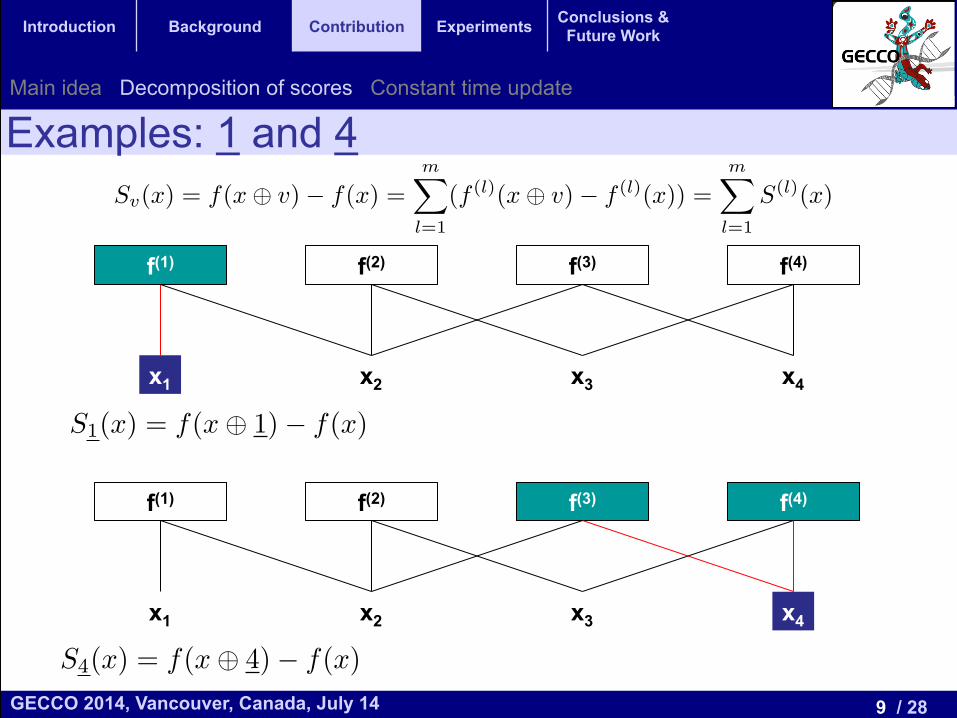
Examples: 1 and 4
f(1) f(2) f(3) f(4)
x1 x2 x3 x4
r = 1 n
r = 2�n2
�
r = 3�n3
�
r
�nr
�
BallPr
i=1
�ni
�
S1(x) = f(x� 1)� f(x)
Sv(x) = f(x� v)� f(x) =mX
l=1
(f (l)(x� v)� f
(l)(x)) =mX
l=1
S
(l)(x)
1
r = 1 n
r = 2�n2
�
r = 3�n3
�
r
�nr
�
BallPr
i=1
�ni
�
S1(x) = f(x� 1)� f(x)
Sv(x) = f(x� v)� f(x) =mX
l=1
(f (l)(x� v)� f
(l)(x)) =mX
l=1
S
(l)(x)
1
f(1) f(2) f(3) f(4)
x1 x2 x3 x4
r = 1 n
r = 2�n2
�
r = 3�n3
�
r
�nr
�
BallPr
i=1
�ni
�
S1(x) = f(x� 1)� f(x)
Sv(x) = f(x� v)� f(x) =mX
l=1
(f (l)(x� v)� f
(l)(x)) =mX
l=1
S
(l)(x)
S4(x) = f(x� 4)� f(x)
1
Main idea Decomposition of scores Constant time update
10 / 28 GECCO 2014, Vancouver, Canada, July 14
Introduction Background Contribution Experiments Conclusions & Future Work
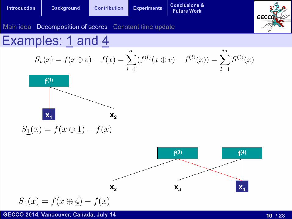
Examples: 1 and 4
f(1)
x1 x2
r = 1 n
r = 2�n2
�
r = 3�n3
�
r
�nr
�
BallPr
i=1
�ni
�
S1(x) = f(x� 1)� f(x)
Sv(x) = f(x� v)� f(x) =mX
l=1
(f (l)(x� v)� f
(l)(x)) =mX
l=1
S
(l)(x)
1
r = 1 n
r = 2�n2
�
r = 3�n3
�
r
�nr
�
BallPr
i=1
�ni
�
S1(x) = f(x� 1)� f(x)
Sv(x) = f(x� v)� f(x) =mX
l=1
(f (l)(x� v)� f
(l)(x)) =mX
l=1
S
(l)(x)
1
f(3) f(4)
x2 x3 x4
r = 1 n
r = 2�n2
�
r = 3�n3
�
r
�nr
�
BallPr
i=1
�ni
�
S1(x) = f(x� 1)� f(x)
Sv(x) = f(x� v)� f(x) =mX
l=1
(f (l)(x� v)� f
(l)(x)) =mX
l=1
S
(l)(x)
S4(x) = f(x� 4)� f(x)
1
Main idea Decomposition of scores Constant time update
11 / 28 GECCO 2014, Vancouver, Canada, July 14
Introduction Background Contribution Experiments Conclusions & Future Work
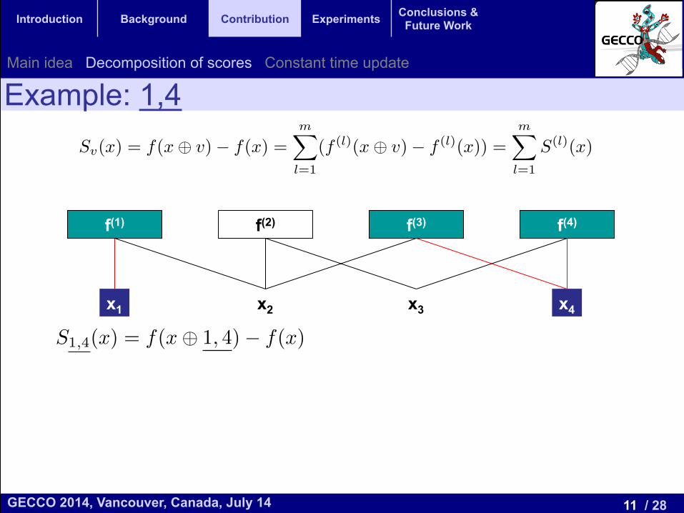
Example: 1,4
f(1) f(2) f(3) f(4)
x1 x2 x3 x4
r = 1 n
r = 2�n2
�
r = 3�n3
�
r
�nr
�
BallPr
i=1
�ni
�
S1(x) = f(x� 1)� f(x)
Sv(x) = f(x� v)� f(x) =mX
l=1
(f (l)(x� v)� f
(l)(x)) =mX
l=1
S
(l)(x)
1
r = 1 n
r = 2�n2
�
r = 3�n3
�
r
�nr
�
BallPr
i=1
�ni
�
S1(x) = f(x� 1)� f(x)
Sv(x) = f(x� v)� f(x) =mX
l=1
(f (l)(x� v)� f
(l)(x)) =mX
l=1
S
(l)(x)
S4(x) = f(x� 4)� f(x)
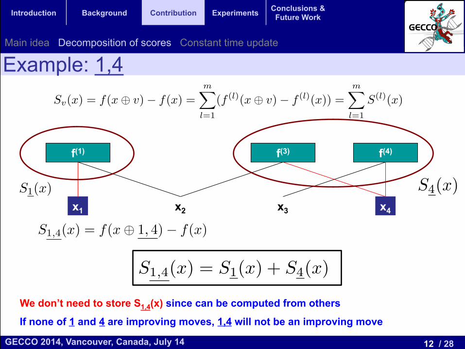
S1,4(x) = f(x� 1, 4)� f(x)
1
Main idea Decomposition of scores Constant time update
12 / 28 GECCO 2014, Vancouver, Canada, July 14
Introduction Background Contribution Experiments Conclusions & Future Work
Example: 1,4
f(1) f(3) f(4)
x1 x2 x3 x4
r = 1 n
r = 2�n2
�
r = 3�n3
�
r
�nr
�
BallPr
i=1
�ni
�
S1(x) = f(x� 1)� f(x)
Sv(x) = f(x� v)� f(x) =mX
l=1
(f (l)(x� v)� f
(l)(x)) =mX
l=1
S
(l)(x)
1
r = 1 n
r = 2�n2
�
r = 3�n3
�
r
�nr
�
BallPr
i=1
�ni
�
S1(x) = f(x� 1)� f(x)
Sv(x) = f(x� v)� f(x) =mX
l=1
(f (l)(x� v)� f
(l)(x)) =mX
l=1
S
(l)(x)
S4(x) = f(x� 4)� f(x)
S1,4(x) = f(x� 1, 4)� f(x)
1
r = 1 n
r = 2�n2
�
r = 3�n3
�
r
�nr
�
BallPr
i=1
�ni
�
S1(x) = f(x� 1)� f(x)
Sv(x) = f(x� v)� f(x) =mX
l=1
(f (l)(x� v)� f
(l)(x)) =mX
l=1
S
(l)(x)
1
r = 1 n
r = 2�n2
�
r = 3�n3
�
r
�nr
�
BallPr
i=1
�ni
�
S1(x) = f(x� 1)� f(x)
Sv(x) = f(x� v)� f(x) =mX
l=1
(f (l)(x� v)� f
(l)(x)) =mX
l=1
S
(l)(x)
S4(x) = f(x� 4)� f(x)
1
r = 1 n
r = 2�n2
�
r = 3�n3
�
r
�nr
�
BallPr
i=1
�ni
�
S1(x) = f(x� 1)� f(x)
Sv(x) = f(x� v)� f(x) =mX
l=1
(f (l)(x� v)� f
(l)(x)) =mX
l=1
S
(l)(x)
S4(x) = f(x� 4)� f(x)
S1,4(x) = f(x� 1, 4)� f(x)
S1,4(x) = S1(x) + S4(x)
1
We don’t need to store S1,4(x) since can be computed from others
If none of 1 and 4 are improving moves, 1,4 will not be an improving move
Main idea Decomposition of scores Constant time update
13 / 28 GECCO 2014, Vancouver, Canada, July 14
Introduction Background Contribution Experiments Conclusions & Future Work
Example: 1,2
r = 1 n
r = 2�n2
�
r = 3�n3
�
r
�nr
�
BallPr
i=1
�ni
�
S1(x) = f(x� 1)� f(x)
Sv(x) = f(x� v)� f(x) =mX
l=1
(f (l)(x� v)� f
(l)(x)) =mX
l=1
S
(l)(x)
S4(x) = f(x� 4)� f(x)
S1,4(x) = f(x� 1, 4)� f(x)
S1,4(x) = S1(x) + S4(x)
S1(x) = f
(1)(x� 1)� f
(1)(x)
1
f(1) f(2) f(3)
x1 x2 x3 x4
f(1) f(2) f(3)
x1 x2 x3 x4
f(1)
x1 x2
r = 1 n
r = 2�n2
�
r = 3�n3
�
r
�nr
�
BallPr
i=1
�ni
�
S1(x) = f(x� 1)� f(x)
Sv(x) = f(x� v)� f(x) =mX
l=1
(f (l)(x� v)� f
(l)(x)) =mX
l=1
S
(l)(x)
S4(x) = f(x� 4)� f(x)
S1,4(x) = f(x� 1, 4)� f(x)
S1,4(x) = S1(x) + S4(x)
S1(x) = f
(1)(x� 1)� f
(1)(x)
S2(x) = f
(1)(x� 2)� f
(1)(x) + f
(2)(x� 2)� f
(2)(x) + f
(3)(x� 2)� f
(3)(x)
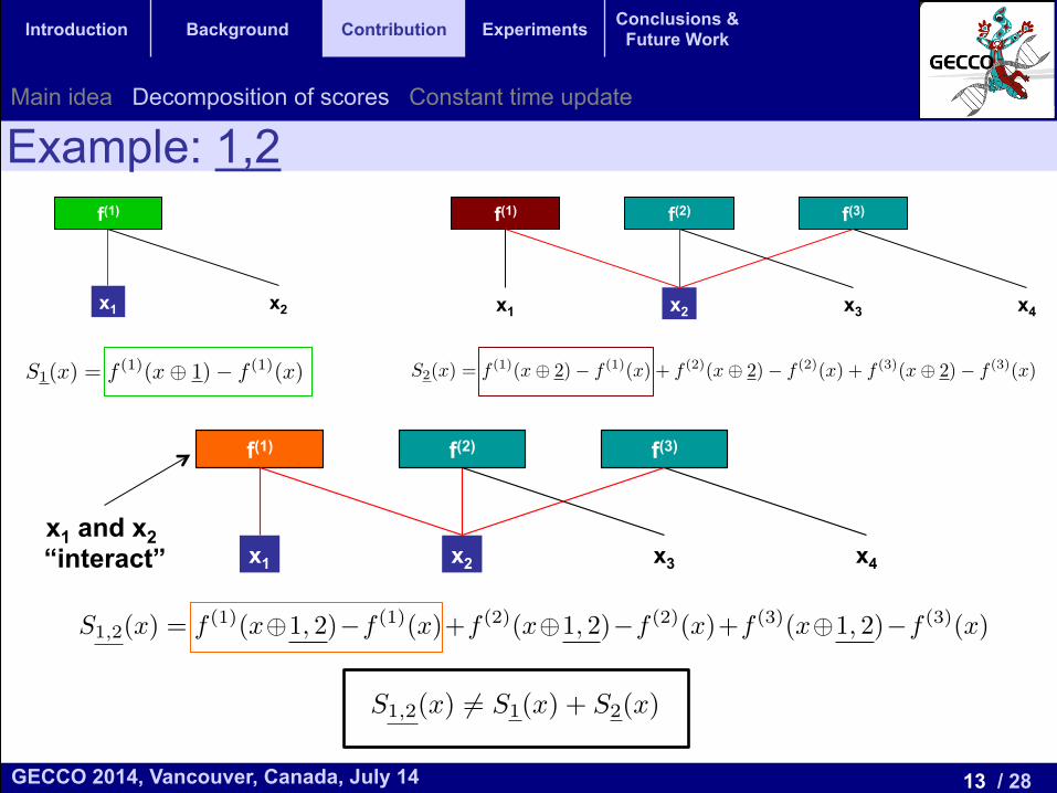
S1,2(x) = f
(1)(x�1, 2)�f
(1)(x)+f
(2)(x�1, 2)�f
(2)(x)+f
(3)(x�1, 2)�f
(3)(x)
S1,2(x) 6= S1(x) + S2(x)
1
r = 1 n
r = 2�n2
�
r = 3�n3
�
r
�nr
�
BallPr
i=1
�ni
�
S1(x) = f(x� 1)� f(x)
Sv(x) = f(x� v)� f(x) =mX
l=1
(f (l)(x� v)� f
(l)(x)) =mX
l=1
S
(l)(x)
S4(x) = f(x� 4)� f(x)
S1,4(x) = f(x� 1, 4)� f(x)
S1,4(x) = S1(x) + S4(x)
S1(x) = f
(1)(x� 1)� f
(1)(x)
S2(x) = f
(1)(x� 2)� f
(1)(x) + f
(2)(x� 2)� f
(2)(x) + f
(3)(x� 2)� f
(3)(x)
S1,2(x) = f
(1)(x�1, 2)�f
(1)(x)+f
(2)(x�1, 2)�f
(2)(x)+f
(3)(x�1, 2)�f
(3)(x)
S1,2(x) 6= S1(x) + S2(x)
1
x1 and x2 “interact”
Main idea Decomposition of scores Constant time update
14 / 28 GECCO 2014, Vancouver, Canada, July 14
Introduction Background Contribution Experiments Conclusions & Future Work
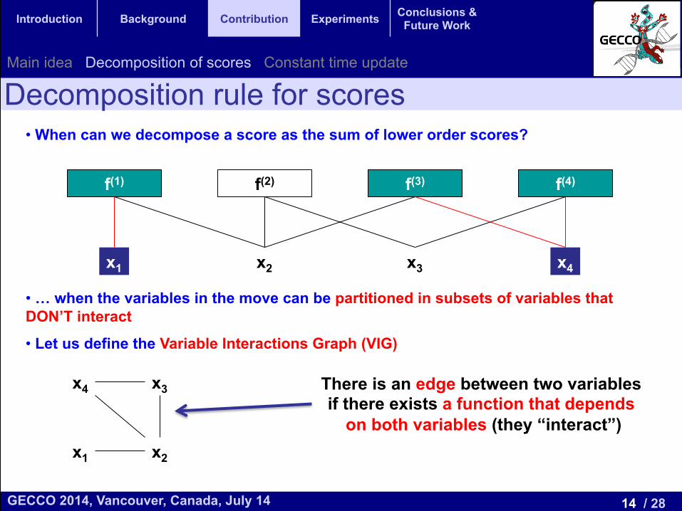
Decomposition rule for scores • When can we decompose a score as the sum of lower order scores?
• … when the variables in the move can be partitioned in subsets of variables that DON’T interact
• Let us define the Variable Interactions Graph (VIG)
f(1) f(2) f(3) f(4)
x1 x2 x3 x4
There is an edge between two variables if there exists a function that depends
on both variables (they “interact”)
x4 x3
x1 x2
Main idea Decomposition of scores Constant time update
15 / 28 GECCO 2014, Vancouver, Canada, July 14
Introduction Background Contribution Experiments Conclusions & Future Work
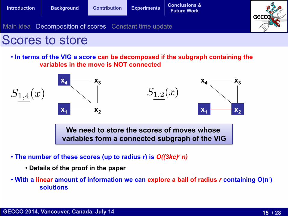
Scores to store • In terms of the VIG a score can be decomposed if the subgraph containing the
variables in the move is NOT connected
• The number of these scores (up to radius r) is O((3kc)r n)
• Details of the proof in the paper
• With a linear amount of information we can explore a ball of radius r containing O(nr) solutions
x4 x3
x1 x2
x4 x3
x1 x2
r = 1 n
r = 2�n2
�
r = 3�n3
�
r
�nr
�
BallPr
i=1
�ni
�
S1(x) = f(x� 1)� f(x)
Sv(x) = f(x� v)� f(x) =mX
l=1
(f (l)(x� v)� f
(l)(x)) =mX
l=1
S
(l)(x)
S4(x) = f(x� 4)� f(x)
S1,4(x) = f(x� 1, 4)� f(x)
S1,4(x) = S1(x) + S4(x)
S1(x) = f
(1)(x� 1)� f
(1)(x)
S2(x) = f
(1)(x� 2)� f
(1)(x) + f
(2)(x� 2)� f
(2)(x) + f
(3)(x� 2)� f
(3)(x)
S1,2(x) = f
(1)(x�1, 2)�f
(1)(x)+f
(2)(x�1, 2)�f
(2)(x)+f
(3)(x�1, 2)�f
(3)(x)
S1,2(x) 6= S1(x) + S2(x)
1
r = 1 n
r = 2�n2
�
r = 3�n3
�
r
�nr
�
BallPr
i=1
�ni
�
S1(x) = f(x� 1)� f(x)
Sv(x) = f(x� v)� f(x) =mX
l=1
(f (l)(x� v)� f
(l)(x)) =mX
l=1
S
(l)(x)
S4(x) = f(x� 4)� f(x)
S1,4(x) = f(x� 1, 4)� f(x)
S1,4(x) = S1(x) + S4(x)
1
We need to store the scores of moves whose variables form a connected subgraph of the VIG
Main idea Decomposition of scores Constant time update
16 / 28 GECCO 2014, Vancouver, Canada, July 14
Introduction Background Contribution Experiments Conclusions & Future Work
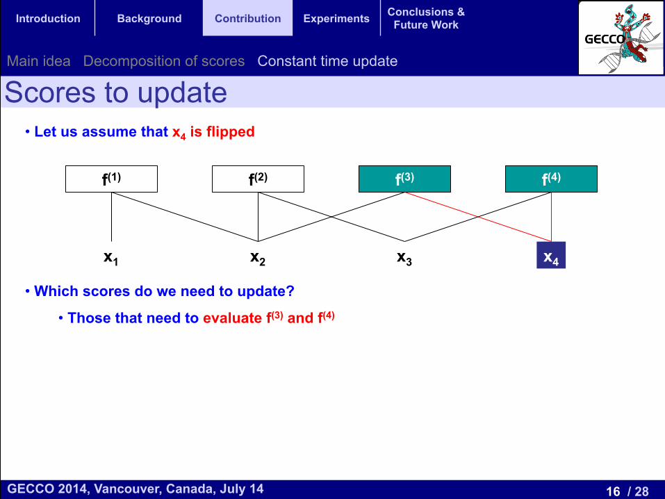
Scores to update • Let us assume that x4 is flipped
• Which scores do we need to update?
• Those that need to evaluate f(3) and f(4)
f(1) f(2) f(3) f(4)
x1 x2 x3 x4
Main idea Decomposition of scores Constant time update
17 / 28 GECCO 2014, Vancouver, Canada, July 14
Introduction Background Contribution Experiments Conclusions & Future Work
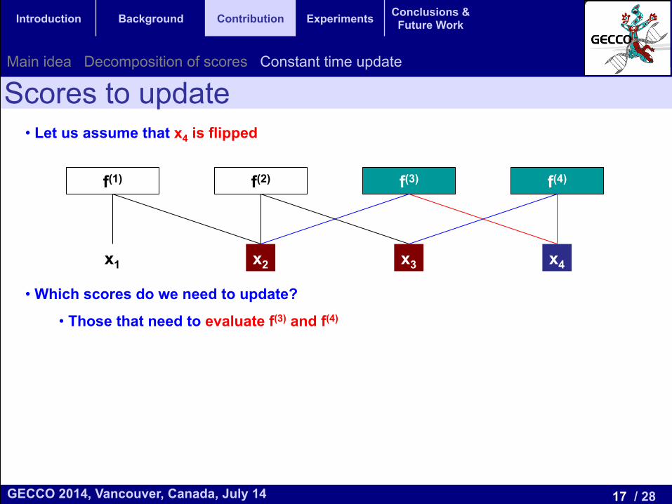
Scores to update • Let us assume that x4 is flipped
• Which scores do we need to update?
• Those that need to evaluate f(3) and f(4)
f(1) f(2) f(3) f(4)
x1 x2 x3 x4
Main idea Decomposition of scores Constant time update
18 / 28 GECCO 2014, Vancouver, Canada, July 14
Introduction Background Contribution Experiments Conclusions & Future Work
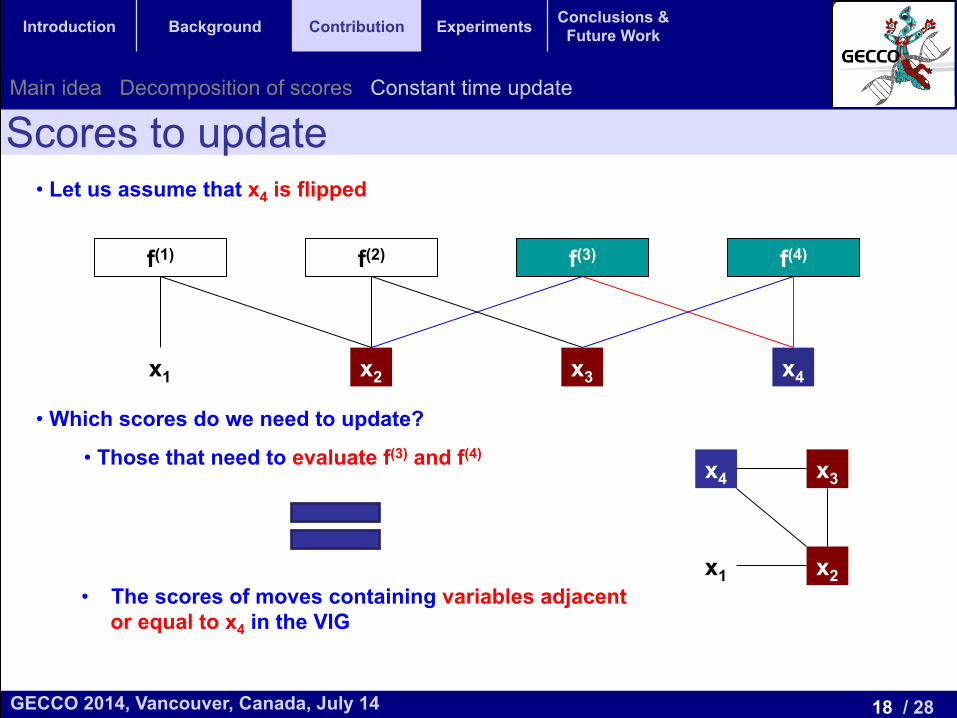
Scores to update • Let us assume that x4 is flipped
• Which scores do we need to update?
• Those that need to evaluate f(3) and f(4)
f(1) f(2) f(3) f(4)
x1 x2 x3 x4
Main idea Decomposition of scores Constant time update
x4 x3
x1 x2 • The scores of moves containing variables adjacent
or equal to x4 in the VIG
19 / 28 GECCO 2014, Vancouver, Canada, July 14
Introduction Background Contribution Experiments Conclusions & Future Work
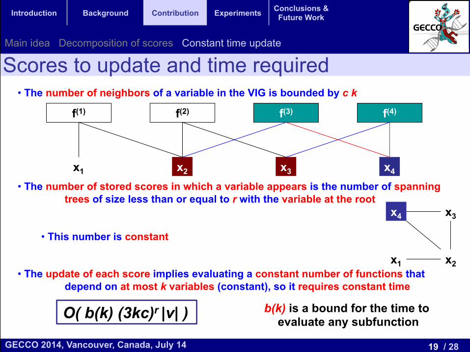
Scores to update and time required • The number of neighbors of a variable in the VIG is bounded by c k
• The number of stored scores in which a variable appears is the number of spanning trees of size less than or equal to r with the variable at the root
• This number is constant
• The update of each score implies evaluating a constant number of functions that depend on at most k variables (constant), so it requires constant time
x4 x3
x1 x2
O( b(k) (3kc)r |v| ) b(k) is a bound for the time to evaluate any subfunction
Main idea Decomposition of scores Constant time update
f(1) f(2) f(3) f(4)
x1 x2 x3 x4
20 / 28 GECCO 2014, Vancouver, Canada, July 14
Introduction Background Contribution Experiments Conclusions & Future Work
Definition NKq-landscapes Sanity check Random model Next improvement
Why NKq and not NK?
Floating point precision
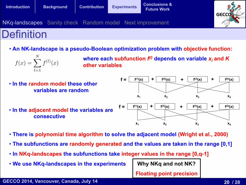
• An NK-landscape is a pseudo-Boolean optimization problem with objective function:
where each subfunction f(l) depends on variable xl and K other variables
• There is polynomial time algorithm to solve the adjacent model (Wright et al., 2000)
• The subfunctions are randomly generated and the values are taken in the range [0,1]
• In NKq-landscapes the subfunctions take integer values in the range [0,q-1]
• We use NKq-landscapes in the experiments
r = 1 n
r = 2�n2
�
r = 3�n3
�
r
�nr
�
BallPr
i=1
�ni
�
S1(x) = f(x� 1)� f(x)
Sv(x) = f(x� v)� f(x) =mX
l=1
(f (l)(x� v)� f
(l)(x)) =mX
l=1
S
(l)(x)
S4(x) = f(x� 4)� f(x)
S1,4(x) = f(x� 1, 4)� f(x)
S1,4(x) = S1(x) + S4(x)
S1(x) = f
(1)(x� 1)� f
(1)(x)
S2(x) = f
(1)(x� 2)� f
(1)(x) + f
(2)(x� 2)� f
(2)(x) + f
(3)(x� 2)� f
(3)(x)
S1,2(x) = f
(1)(x�1, 2)�f
(1)(x)+f
(2)(x�1, 2)�f
(2)(x)+f
(3)(x�1, 2)�f
(3)(x)
S1,2(x) 6= S1(x) + S2(x)
f(x) =NX
l=1
f
(l)(x)
1
f = + + + f(1)(x) f(3)(x) f(2)(x) f(4)(x)
x1 x2 x3 x4
• In the random model these other variables are random
• In the adjacent model the variables are consecutive
f = + + + f(1)(x) f(3)(x) f(2)(x) f(4)(x)
x1 x2 x3 x4

21 / 28 GECCO 2014, Vancouver, Canada, July 14
Introduction Background Contribution Experiments Conclusions & Future Work
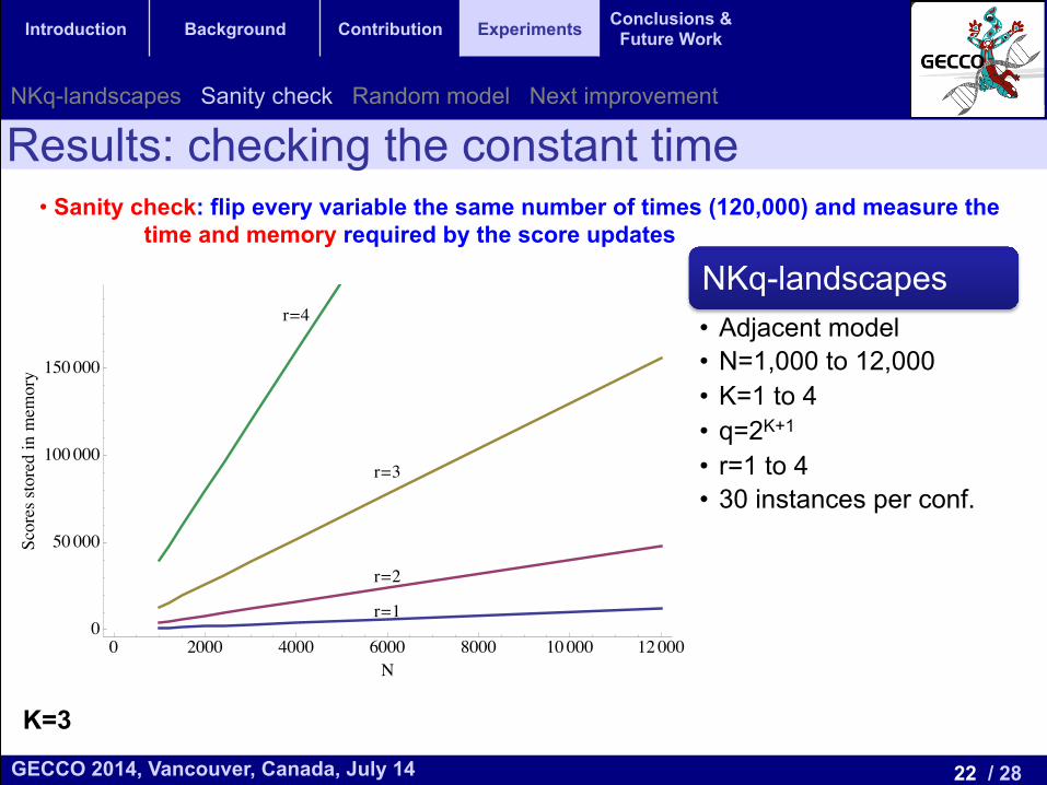
Results: checking the constant time • Sanity check: flip every variable the same number of times (120,000) and measure the
time and memory required by the score updates
NKq-landscapes • Adjacent model • N=1,000 to 12,000 • K=1 to 4 • q=2K+1
• r=1 to 4 • 30 instances per conf.
K=3
r=1r=2
r=3
r=4
0 2000 4000 6000 8000 10000 120000
5
10
15
20
N
TimeHsL
NKq-landscapes Sanity check Random model Next improvement
22 / 28 GECCO 2014, Vancouver, Canada, July 14
Introduction Background Contribution Experiments Conclusions & Future Work
Results: checking the constant time • Sanity check: flip every variable the same number of times (120,000) and measure the
time and memory required by the score updates
NKq-landscapes • Adjacent model • N=1,000 to 12,000 • K=1 to 4 • q=2K+1
• r=1 to 4 • 30 instances per conf.
K=3
r=1
r=2
r=3
r=4
0 2000 4000 6000 8000 10000 120000
50000
100000
150000
N
Scoresstoredinmemory
NKq-landscapes Sanity check Random model Next improvement
23 / 28 GECCO 2014, Vancouver, Canada, July 14
Introduction Background Contribution Experiments Conclusions & Future Work
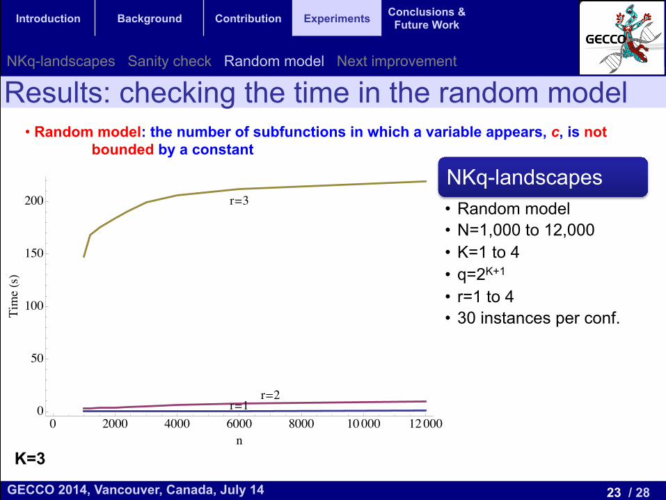
Results: checking the time in the random model • Random model: the number of subfunctions in which a variable appears, c, is not
bounded by a constant
NKq-landscapes • Random model • N=1,000 to 12,000 • K=1 to 4 • q=2K+1
• r=1 to 4 • 30 instances per conf.
K=3
r=1r=2
r=3
0 2000 4000 6000 8000 10000 120000
50
100
150
200
n
TimeHsL
NKq-landscapes Sanity check Random model Next improvement
24 / 28 GECCO 2014, Vancouver, Canada, July 14
Introduction Background Contribution Experiments Conclusions & Future Work
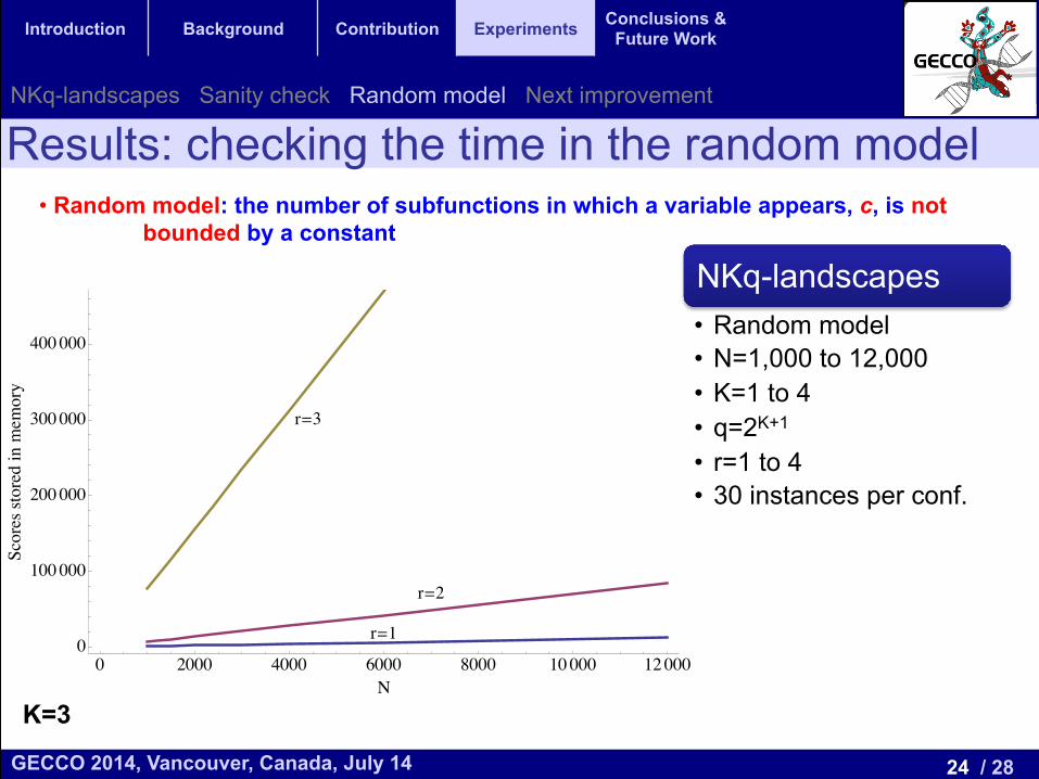
Results: checking the time in the random model • Random model: the number of subfunctions in which a variable appears, c, is not
bounded by a constant
NKq-landscapes • Random model • N=1,000 to 12,000 • K=1 to 4 • q=2K+1
• r=1 to 4 • 30 instances per conf.
K=3
r=1
r=2
r=3
0 2000 4000 6000 8000 10000 120000
100000
200000
300000
400000
N
Scoresstoredinmemory
NKq-landscapes Sanity check Random model Next improvement
25 / 28 GECCO 2014, Vancouver, Canada, July 14
Introduction Background Contribution Experiments Conclusions & Future Work
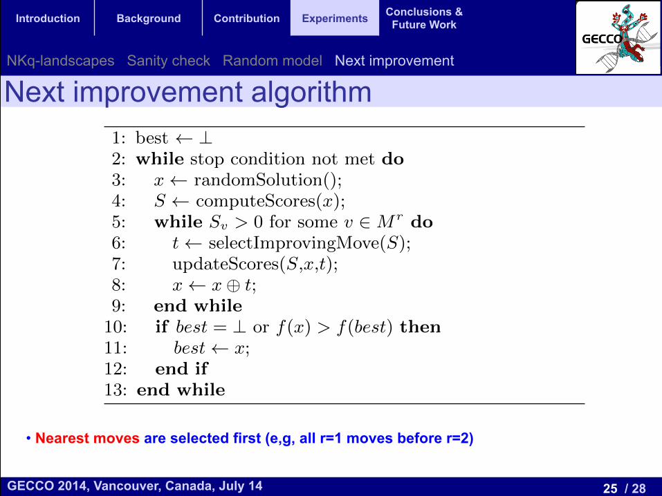
Next improvement algorithm
• Nearest moves are selected first (e,g, all r=1 moves before r=2)
depends only on at most k Boolean variables and each vari-able appears in at most c subfunctions. Let the graph G bethe variable interaction graph of f and Mr the set of movesv 2 Br up to order r such that G[v] is a connected graph.Then:
• The cardinality of Mr is O((3kc)rn).
• We only need to check the Scores Sv(x) with v 2 Mr
of the current solution x to determine the presence ofan improving move in a ball of radius r around x. Ifthe Scores are stored in memory this check requiresconstant time.
• The Scores Sv(x) for v 2Mr can be updated when wemove from one solution x to x � t using Algorithm 1in time O(b(k)(3kc)r|t|), where b(k) is a bound of thetime required to evaluate any subfunction f (l). Thistime is independent of n if k, r and c are independentof n.
4. THE HAMMING-BALL HILL CLIMBERThe e�cient Scores update of Algorithm 1 can be used
in combination with any trajectory-based method like, It-erated Local Search or Tabu Search. In this section we de-scribe a next ascent hill climber based on it. The proposedhill climber is shown in Algorithm 3. We assume maximiza-tion and for this reason we say that it is an “ascent” hillclimber. However, the algorithm can consider minimizationjust changing the > operators in lines 5 and 10 by < oper-ators. In the algorithm, variable best stores the best foundsolution at any given time. The algorithm starts by assign-ing the special value ?, which means “no solution” to best.Next, it enters a loop that is repeated until the stoppingcondition is met. Each run of the loop body is an ascentstarting from a random solution in the search space. In theloop, once a random solution has been selected and stored inx, the algorithm computes the Scores Sv(x) for all v 2 Mr
using the expression (6). The inner loop starting in line 5implements the next ascent. While an improving move ex-ists (Sv > 0 for some v 2 Mr), the algorithm selects oneof the improving moves t (line 6), updates the Scores usingAlgorithm 1 (line 7) and changes the current solution by thenew one (line 8).
Algorithm 3 Hamming-ball next ascent.
1: best ?2: while stop condition not met do3: x randomSolution();4: S computeScores(x);5: while Sv > 0 for some v 2Mr do6: t selectImprovingMove(S);7: updateScores(S,x,t);8: x x� t;9: end while10: if best = ? or f(x) > f(best) then11: best x;12: end if13: end while
Regarding the selection of the improving move, our ap-proach in the experiments was to select always the one withthe lowest Hamming distance to the current solution, that
is, the lowest value of |t|. The main reason for selecting thenearest improving move is that, as stated by Theorem 1,the time required for updating the Scores is proportional to|t|. Thus, the nearest improving move is the fastest movein our algorithm. This selection can be done in constanttime, since the classification of the moves as improving ornon-improving can be done when the Scores are calculatedand the Scores can be added to di↵erent lists depending onthe distance to the current solution.From the point of view of computation time, we expect
the statements between lines 6 and 8 to run in a time thatis independent of n. However, this time depends on k, cand r, where r is the only algorithm-dependent parameter(the others depend on the problem instance). According toTheorem 1, the time is exponential in r. Therefore, we haveto be especially careful when we set the radius of the ball.Lines 3 and 4 are expected to run in linear time with respectto n, since the number of Scores (and variables) is linear.Let us now consider the quality of the solutions obtained
by the algorithm when we change r. Let us pick two radiifor the ball: r1 < r2. Let us imagine that two ascents startfrom the same solution, one in each algorithm. Both in-stances of the algorithm will visit the same solutions untilthe algorithm with radius r1 gets stuck in a local optimumor a plateau. In this case, however, the algorithm with r2,which is considering a larger neighborhood, could find an im-proving move and could continue. Thus, we expect longerascents and better quality solutions at the end of the ascentsfor larger values of r.The fitness value of the best solution is a non-decreasing
function of the time. As we increase r we expect bettersolutions at the end of the ascents, but the time spent in eachascent is also longer. It could happen that an instance of thealgorithm with a lower value for r can reach better solutionsearlier just because it is faster and finds an appropriate pathjoining lower distance moves. This fact makes impossible toset an a priori value for r that is valid for all the problemsand instances. In the experimental section we will discussthis issue again on the results.
5. EXPERIMENTAL RESULTSIn this section we present experimental results obtained
with the Hamming-ball next ascent. For the experiments weused NKq-landscapes. They are randomly generated func-tions that are specially interesting because it is possible tochange their ruggedness and neutrality changing K and q,respectively. The objective function is:
f(x) =nX
l=1
f (l)(x), (10)
where each subfunction f (l) depends on variable xl and otherK variables and we have k = K +1. These variables can berandomly selected from the remaining n�1, which yields therandom-model NKq-landscapes. If the variables for subfunc-tion f (l) are {xl, xl+1, . . . , xl+K} with sum modulo n (andindices in the range 1 to n), then we have the adjacent-modelNKq-landscapes. The latter has the advantage that a globaloptimum can be found in polynomial time using an algo-rithm proposed by Wright et al. [10], but also the numberof subfunctions depending on a given variable is constant:c = k = K + 1. In the random-model there is no constantbound for the number of subfunctions in which the variables
NKq-landscapes Sanity check Random model Next improvement
26 / 28 GECCO 2014, Vancouver, Canada, July 14
Introduction Background Contribution Experiments Conclusions & Future Work
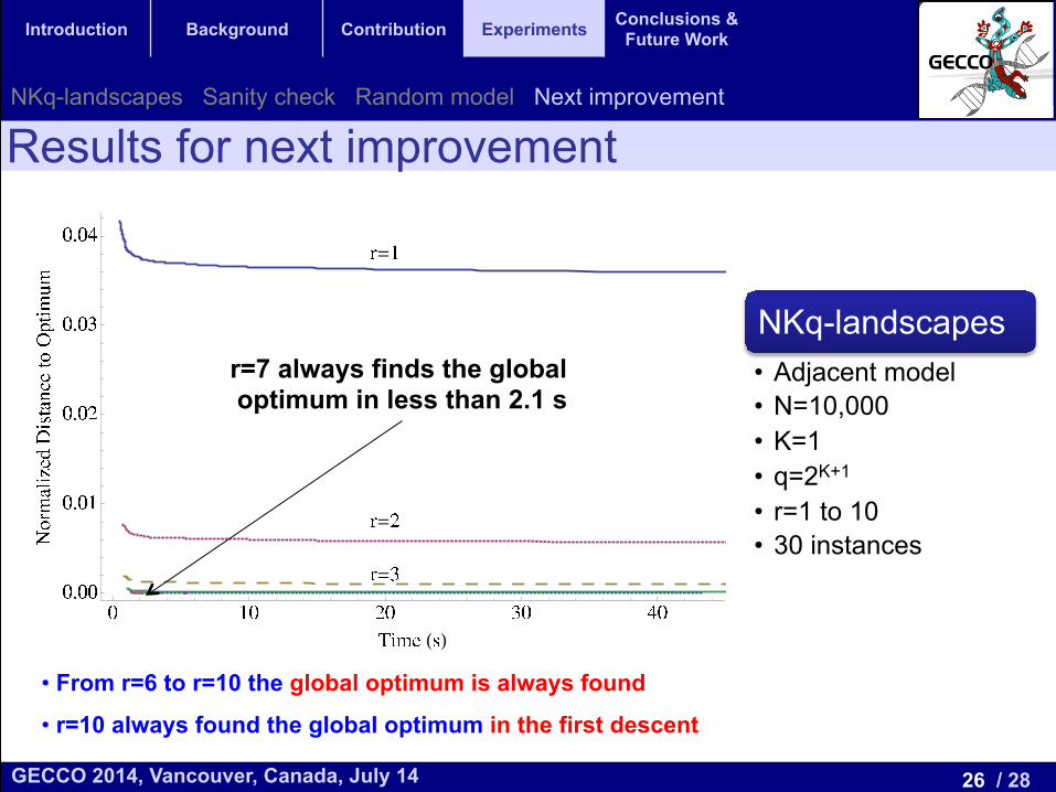
Results for next improvement
way with n as illustrated in Figure 5(b), although in theorythe increase could be more than linear.
(a) Time for Score updates (b) Scores stored in memory
(c) Maximum subfunctions a↵ected, c
Figure 5: Time, Scores and maximum numberof subfunctions a↵ected by a single variable forrandom-model NKq-landscapes.
5.2 On the Quality of the SolutionsIn Section 4 we argued that an ascent of the Hamming-
ball next ascent with radius r1 < r2 cannot obtain a bettersolution than an ascent starting from the same solution butusing radius r2. As a consequence, if the stopping condi-tion of Algorithm 3 is to reach a fixed number of ascents,then we expect the quality of the solutions using r2 to beno worse than the quality of the solutions when r1 is theradius. However, larger radius also means longer executiontime, not only for the Scores update but also for the di↵er-ent initialization procedures. If the stopping condition is toreach a fixed amount of time we cannot say which radius isthe best option. The experiments in this section illustratewhat happens in this case of NKq-landscapes.
Let us start analyzing the adjacent-model. We fix n =10, 000 and generated 30 instances for each combination ofKused. We run the algorithm for 120 seconds in all the cases.Figure 6 shows the average fitness over the 30 instances ofthe best solution found by the algorithms against the elapsedtime from the start of the search. The radius used are r = 1to 6. In the figure K = 2 and q = 8. We can observethat using larger values for r the algorithm is able to findbetter solutions at any time. In the figure, it is clear that thealgorithm with r = 1 cannot reach in 120 seconds the qualityof the solutions found by the one with r = 2 at the beginningof its search. The same applies in the comparison with otherradii. We can conclude that, in this example and for r = 1to 6, increasing the value of r we obtain progressively betteralgorithms, even when the stopping condition is a time limit.
However, this improvement has also limitations. The gainin the quality of the solutions when we increase r from 1 to 2is larger than the gain when we increase r from 2 to 3. Sincethe fitness value of the global optimum acts as a bound forthe quality of the solutions, there must be an r value forwhich there is no gain. At this point, increasing r we canonly penalize the e�cacy of the algorithm because the run-
Figure 6: Best solution fitness over time for theHamming-ball next ascent in adjacent-model NKq-landscapes.
time will still increase. To check this fact, we show in Fig-ure 7 the normalized distance to the global optimum of theHamming-ball next ascent for di↵erent radii (note that weare maximizing the objective function, but minimizing thedistance to the global optimum). The points are averagesover 30 random instances with n = 10, 000, K = 1, q = 4and r = 1 to 10. The algorithms were run for 120 seconds.The normalized distance to the optimum, nd, is:
nd(x) =f⇤ � f(x)
f⇤ , (11)
where f⇤ is the fitness value of the global optimum, com-puted using the algorithm by Wright et al. [10].
Figure 7: Normalized distance to the global opti-mum for the Hamming-ball next ascent.
With r = 1 the algorithm is approximately within 3.6% ofthe global optimum after 20 seconds. As we increase r, thealgorithms get closer to the global optimum and the gainsshrink. For r = 3 the results are withing 0.2% of the globaloptimum. For r > 3 the di↵erences are so small that cannotbe observed in the plot. For r � 6 an optimal solution isfound in all the instances. For r = 6 the solution is foundin 3.7 seconds. For r = 7 it is found in 2.1 seconds, and thisis the fastest algorithm. For r = 8, 9 and 10 the algorithmrequires 2.8 s, 3.4 s, and 5 s to find the optimal solution. Forr = 10 the algorithm finds an optimal solution in the firstascent for all the instances.Let us now consider a random NKq-Landscape, one that
does not use adjacent interacting variables. In Figure 8 we
NKq-landscapes • Adjacent model • N=10,000 • K=1 • q=2K+1
• r=1 to 10 • 30 instances
• From r=6 to r=10 the global optimum is always found
• r=10 always found the global optimum in the first descent
r=7 always finds the global optimum in less than 2.1 s
NKq-landscapes Sanity check Random model Next improvement
27 / 28 GECCO 2014, Vancouver, Canada, July 14
Introduction Background Contribution Experiments Conclusions & Future Work
Conclusions and Future Work Conclusions & Future Work
• We can identify improving moves in a ball of radius r around a solution in constant time (independent of n)
• The space required to store the information (scores) is linear in the size of the problem n
• This information can be used to design efficient search algorithms
Conclusions
• Random restarts are costly, study the applicability of soft restarts
• Application to other pseudo-Boolean problems like MAX-kSAT • Include clever strategies to escape from local optima
Future Work

28 / 28 GECCO 2014, Vancouver, Canada, July 14
Acknowledgements
Efficient Identification of Improving Moves in a Ball for Pseudo-Boolean Problems