efficient calculation of counterparty exposure … books/201003 efficient calculation... · 2...

1

Discussions of counterparty credit have long recognised that it is a dual contingency risk. An institution experiences exposure to po-tential credit loss when a counterparty loses money on its bilateral trades with the institution. This creates positive mark-to-market values on the institution’s balance sheet reflecting the present value of money owed by the counterparty. Actual realised losses (credit risk rather than just credit exposure) require that the counterparty default after having experienced losses on its bilateral portfolio of trades with the institution. If the likelihood of default is statistically independent of the mar-ket events giving rise to exposure, it is valid to calculate expected credit losses by simulating expected exposure separately and then multiplying by the likelihood of default. Unfortunately, this is not a valid approach if default and exposure are correlated (either posi-tively or negatively) with each other. This chapter describes a means of simulating exposure conditional on default of a counterparty. The expected value of such conditional exposure can then be multiplied by the probability of default to derive a statistically valid estimate of expected loss even when exposure and default are correlated. This makes derivation of expected loss no more computationally bur-densome than a standard unconditional exposure simulation.

INTRODUCTIONSimulation of credit exposure to derivative counterparties dates back to the mid-1980s. It was initially prompted by the need to in-

3

Efficient Calculation of Counterparty Exposure Conditional on DefaultDavid M. Rowe, Philip Koop, Daniel Travers

SunGard

2

COUNTERPARTY CREDIT RISK

clude a provision in the Basel I Capital Accord for potential credit losses on banks’ rapidly growing derivative market-making activi-ties. Early analysis focused on individual interest rate swaps and foreign exchange transactions, and was designed to provide an em-pirical basis for the parameters in what came to be known as the mark-to-market plus add-on approach. This type of calculation was originally designed as a simple way for banks to derive their total potential credit exposure to all derivative counterparties. An unfor-tunate effect of implementing this approach in the Basel I rules was that nearly all banks proceeded to implement a similar (although often more conservative) calculation for measuring and controlling potential credit exposure to individual counterparties. Arguably, this delayed serious efforts to develop more realistic exposure mea-surement techniques for many years. In the early days, application of netting was not legally certain, even in major G7 economies. Thus, the simple addition of assess-ments for single transactions did not introduce a serious distortion. As netting became more widely recognised in legislation and case law precedents, some means of reflecting this risk-reducing phe-nomenon in credit assessments became more urgent. Even then, however, this often took the form of some easing of the parameters in the mark-to-market plus add-on approach, rather than develop-ing a full-blown simulation process. A few banks began work on exposure simulation systems in the early 1990s.1 Such efforts were necessarily hampered by limitations on the computing capacity that was commercially practical to de-vote to such systems. The focus was primarily on making significant improvements to the mark-to-market plus add-on approach, which was quite a modest goal given the well-known shortcoming of that technique. In general, the philosophy was to err on the side of con-servatism so that simulations would not understate exposure versus approved limits. Achieving significantly greater sophistication was deemed commercially impractical and of marginal importance. Much has changed in the past 20 years, both in the derivative market itself and in the technology available to support related risk systems. The biggest change in the derivative market has been the explosion of transactions for which some form of credit risk is the primary variable driving the value. Single-name credit default

3

EFFICIENT CALCULATION OF COUNTERPARTY EXPOSURE CONDITIONAL ON DEFAULT

swaps and a vast array of structured credit securities, both primary and synthetic, have introduced a new dimension of complexity to valuation and to counterparty exposure simulation. More recently, the crisis in financial markets that erupted in 2008 sharpened the recognition of counterparty risk as a very real threat that must be taken seriously. This has generated increased demand for more so-phisticated exposure measures and a desire to price for counter-party credit risk in the normal course of daily trading activity. Fortunately, some advances in technology since the turn of the century are well suited to supporting these aspirations for coun-terparty credit risk analysis that is both timelier and more sophisti-cated. The two advances with the most to offer are:

o

o

grid computing that enables massive parallel processing; and64-bit architecture that supports a massive expansion in address-able memory capacity.

While these are not extremely recent innovations, they have only become proven, commercially attractive, mainstream technologies in recent years. Furthermore, as with all major advances in hard-ware architecture, pre-existing software has had to undergo signifi-cant revisions to take full advantage of the new possibilities. The combination of these hardware advances and progressive software adaptation has created dramatic new opportunities for improved management of counterparty credit risk. For the first time it is com-mercially feasible to deploy incremental Monte Carlo simulation as a means of assessing the exposure impact of a proposed new deal sufficiently rapidly to provide trading decision support. This is es-sential if traders are going to be charged for the incremental expect-ed credit default losses implied by their trades – credit valuation adjustment (CVA) – and for the capital to provide a cushion against potential unexpected credit losses. This chapter focuses on an ef-ficient derivation of the exposure at default (EAD) appropriate for input into the economic capital calculation which is sensitive to non-zero correlation between exposure and the probability of default.

WRONG-WAY AND RIGHT-WAY RISKWrong-way credit risk burst into market consciousness in the midst of the Asian currency crisis of 1997–98. Many Asian corporations

4


had borrowed in G7 currencies, most often US dollars or yen. If their revenues were primarily in domestic currency, this presented a major foreign exchange risk. Depreciation of these borrowers’ local currency would significantly increase their effective debt burden. To alleviate this contingency, many such corporations hedged their for-eign exchange risk in the currency swap market. Furthermore, they often executed these transactions with Western banks. Having exe-cuted these trades with an Asian corporation, the Western bank now held a sizable open foreign exchange position that they needed to hedge. In looking for suitable professional counterparties, the most active players often would be money centre banks in the original borrower’s home country. In executing such a hedge, however, the Western banks took on classic wrong-way risk. The Western bank was paying the Asian currency and receiving its own currency from an Asian bank. When several Asian currencies depreciated dra-matically, the value of these trades moved decisively in favour of the Western banks just as the local economies of their counterparty banks were falling into crisis. The local turmoil resulted in several Asian bank failures and consequent credit losses for the Western bank counterparties to these significantly in-the-money trades. As always, experience was a harsh but effective teacher. Since the derivative credit losses stemming from the largely inadvertent build-up of wrong-way risk prior to the Asian currency crisis, the correla-tion between exposure and default probability has remained a lively topic for debate. Since most end-users are primarily attempting to hedge fundamental business risks most of the time, there should be a strong presumption that most derivative positions represent right-way risk. An example is an airline entering into a swap where they pay fixed and receive a floating payment based on the future price of jet fuel. They lose money on the swap when jet fuel prices fall, but this price decline tends to increase the profitability of their core business, making them a better credit risk. Even though most swaps and other derivatives are used to hedge fundamental business risks, the Asian crisis and its associated losses drove home the realisation that this cannot be taken for granted in any given bilateral portfolio.

IMPLICATIONS FOR CALCULATION OF ECONOMIC CAPITALIn general, we think of expected credit losses as the product of the probability of default times expected exposure (adjusted for expect-

5


ed recoveries). This is quite correct if exposure is static and prede-termined. It also is correct if we can assume that random exposure is uncorrelated with the probability of counterparty default. As not-ed in the previous section, however, such statistical independence between exposure and default will tend to be rare. In most cases it is to be expected that exposure is negatively (ie, favourably) cor-related with the likelihood of default. If a counterparty is hedging a fundamental business risk, the bank will tend to make money on their bilateral trades when the fundamental economic factors are favourable to the counterparty’s business, thereby reducing the probability of default. In other, probably less likely but potentially important, situations the toxic combination of rising exposure and rising default probability needs to be recognised. In calculating unexpected losses used for deriving economic capital, it is similarly important not to assume the independence of exposure and probability of default, as these unlikely but toxic cases of wrong-way risk may have an even greater impact on the tail losses driving trading book economic capital than on the level of expected loss. In the discussion that follows, we first consider credit defaults as the only driver of economic capital. At the end we briefly describe how the method we propose could be extended to reflect the impact of credit rating transitions short of default. The usual process for dealing with the correlation of exposure and default is to include a credit quality variable in the simulation, and to correlate this with all the market variables that drive the value of trades in the bilateral portfolio. The credit quality variable is then evaluated against a default threshold. For every time point in every simulation, it is then possible to derive the value of the exposure and a binary default/no default indicator for the status of the counterparty. By generating a sufficient number of paths, it is possible to determine what proportion of the time a default oc-curs and the distribution of exposure across those instances when it does. The obvious problem with this “brute force” approach is that it is massively wasteful of computing resources. In the overwhelm-ing majority of instances, for all but the shakiest of counterparties, there will be no default. In these cases the exposure amount is ir-relevant to the credit calculation since no credit loss has occurred. Of course, it is possible to simulate the full set of market drivers,

6


including the credit quality variable, and only calculate the implied exposure if a default has occurred. Even so, given the rarity of a default it would often be necessary to generate a million or more full market scenarios to obtain as few as a thousand instances of de-fault. Our proposal is to take this thought process a step further and simulate the drivers of the portfolio value conditional on the credit quality variable being in default status at a specified time horizon. This approach encounters problems if the desire is to generate a full life of the portfolio analysis since, in such an approach, the require-ment is to capture those situations where default occurs at a given time while not having occurred prior to that time. Nevertheless, for a single period analysis (say at a one-year horizon, commonly used for calculating economic capital) simulating exposure condi-tional on default can lead to a significant reduction in the necessary amount of computation.

THE SIMULATION FRAMEWORKThe analytics behind this approach are as follows. Let the scalar V(t) be the future value of a portfolio of securities as a function of time. For portfolios of practical interest, V(t) is unknown and a fun-damental risk management problem is to estimate its distribution. A common solution to this problem is a Monte Carlo simulation in which V(t) is calculated as a function v of a vector of realisations of a set of stochastic market price processes p(t). These processes are generally modelled mathematically as continuous functions but in the simulation can be realised only at a set of n discrete times t1, t2, … tn. For simplicity, we assume that this set of times is the same for each process. Each Monte Carlo scenario s consists of an equally probable vector of discrete process realisations ps(t) and a corresponding evaluation of Vs(t) = v[ps(t)]. To lighten the notation, the remaining discussion is in the context of a single Monte Carlo scenario. Also, we do not assume any particular form of informa-tion filtration, though most implementations operate in the “natu-ral” filtration. In the framework we are considering, an individual price process P(t) may be of a form which could comprise diffusive, jump and complicated drift components, but all randomness is derived from a vector z of correlated standard normal variables generated at

7


each simulation realisation time. In other words, the value of each process realisation at the kth simulation time P(tk) can be written as a function of zk and the realisation of p(t) at previous simulation times. (The size m of z may be either smaller or larger than the size of p. On the one hand, some processes may have more than one stochastic driver; on the other, some stochastic drivers may be sys-temic and be shared among several processes.) We assume that the correlation matrix Σ of z is the same at each simulation time. In this framework, the form of the individual price processes is quite general, but their possible joint distribution is constrained by the underlying multivariate Gaussian distribution. Despite this limi-tation, the framework is justly popular because of its relative tracta-bility with respect to calibration and implementation. It also is ame-nable to various extensions, one of which we describe in this chapter.

CONDITIONAL SIMULATIONSuppose that at a given simulation time, the m normal variables of z are partitioned into subsets z1 and z2 of sizes q and m - q respectively:

where z2 is fixed in advance. The distribution of z1 conditioned on z2 is the conditional multivariate normal distribution. In general terms (if the variables of z do not have identical, standard normal distri-butions), when z is characterised by the mx1 mean vector μ and the mxm covariance matrix Σ then, conditional on fixed values Z2 of the stochastic vector z2, z1 is a multivariate normal distribution charac-terised by the qx1 mean vector μq and the qxq covariance matrix Σq. If we partition the parameters of the unconstrained stochastic process such that

with dimensions

[qx1], [qxq], [qx(m-q)][(m-q)x1], [(m-q)xq], [(m-q)x(m-q)]

then the parameters of the constrained stochastic process for z1

8


conditional on the realisation Z2 of the stochastic vector z2 can be derived as

(Note that, in general, neither Σ nor Σ22 is positive definite; conse-quently, the inverse of Σ22 must be represented by some approxima-tion such as the Moore-Penrose pseudo-inverse.) The significance of the conditional multivariate normal distribution is that it is not necessary to generate complete scenario realisations of all market processes if we want to restrict our attention to scenarios for which some subset of the processes p(t) (let’s refer to this subset as r(t)) exhibits a particular property. It is sufficient to generate candidates of r(t) alone because we can “fill-in” the complete scenario by con-ditioning the remaining normal draws driving the simulation from the subset of z2 that generates acceptable values for r(t).

CONDITIONING APPLIED TO DEFAULTIn the setting we have described, the processes r(t) represent the credit status process of the counterparty, and we are interested in realisations of r(t) that imply counterparty default. We have stated earlier that in this chapter we restrict our attention to short simula-tion horizons for which a single period default model is suitable. From this perspective, the credit status process can have only two outcomes, namely default and survival. Suppose, then, that we choose a credit status process in which only the terminal value is relevant in deciding default. We will not have a default time to guide us in choosing a particular exposure value in the simulation scenario to use as the exposure at default. For regulatory capital this would be consistent with the use of so-called effective expo-sure, in which exposure is floored at its previous maximum value, as the measure of exposure at default. For economic capital pur-poses, another measure of exposure, such as a simple or a weighted average over the one-year time horizon, may be considered. Why are we interested in a complete realisation of the credit sta-tus process if its terminal value is the only thing that determines default? The reason is that exposure may be path dependent if it arises from some path-dependent valuation feature such as a bar-

9


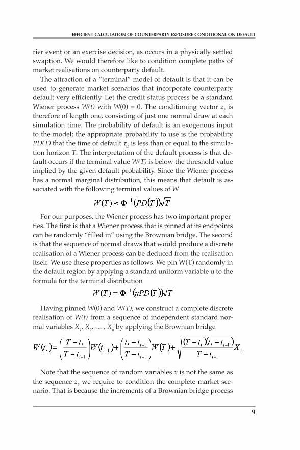
rier event or an exercise decision, as occurs in a physically settled swaption. We would therefore like to condition complete paths of market realisations on counterparty default. The attraction of a “terminal” model of default is that it can be used to generate market scenarios that incorporate counterparty default very efficiently. Let the credit status process be a standard Wiener process W(t) with W(0) = 0. The conditioning vector z2 is therefore of length one, consisting of just one normal draw at each simulation time. The probability of default is an exogenous input to the model; the appropriate probability to use is the probability PD(T) that the time of default τD is less than or equal to the simula-tion horizon T. The interpretation of the default process is that de-fault occurs if the terminal value W(T) is below the threshold value implied by the given default probability. Since the Wiener process has a normal marginal distribution, this means that default is as-sociated with the following terminal values of W

For our purposes, the Wiener process has two important proper-ties. The first is that a Wiener process that is pinned at its endpoints can be randomly “filled in” using the Brownian bridge. The second is that the sequence of normal draws that would produce a discrete realisation of a Wiener process can be deduced from the realisation itself. We use these properties as follows. We pin W(T) randomly in the default region by applying a standard uniform variable u to the formula for the terminal distribution

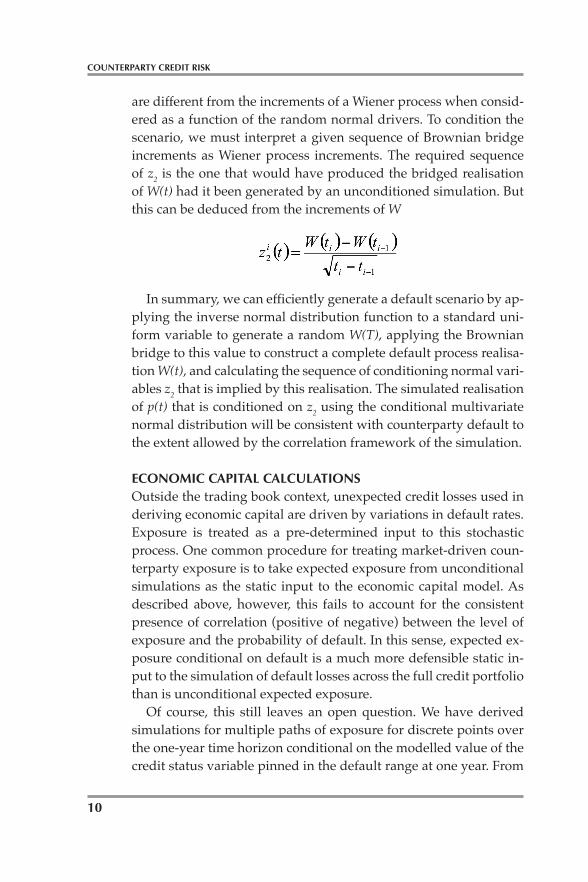
Having pinned W(0) and W(T), we construct a complete discrete realisation of W(t) from a sequence of independent standard nor-mal variables X1, X2, … , Xn by applying the Brownian bridge

Note that the sequence of random variables x is not the same as the sequence z2 we require to condition the complete market sce-nario. That is because the increments of a Brownian bridge process

10


are different from the increments of a Wiener process when consid-ered as a function of the random normal drivers. To condition the scenario, we must interpret a given sequence of Brownian bridge increments as Wiener process increments. The required sequence of z2 is the one that would have produced the bridged realisation of W(t) had it been generated by an unconditioned simulation. But this can be deduced from the increments of W

In summary, we can efficiently generate a default scenario by ap-plying the inverse normal distribution function to a standard uni-form variable to generate a random W(T), applying the Brownian bridge to this value to construct a complete default process realisa-tion W(t), and calculating the sequence of conditioning normal vari-ables z2 that is implied by this realisation. The simulated realisation of p(t) that is conditioned on z2 using the conditional multivariate normal distribution will be consistent with counterparty default to the extent allowed by the correlation framework of the simulation.

ECONOMIC CAPITAL CALCULATIONSOutside the trading book context, unexpected credit losses used in deriving economic capital are driven by variations in default rates. Exposure is treated as a pre-determined input to this stochastic process. One common procedure for treating market-driven coun-terparty exposure is to take expected exposure from unconditional simulations as the static input to the economic capital model. As described above, however, this fails to account for the consistent presence of correlation (positive of negative) between the level of exposure and the probability of default. In this sense, expected ex-posure conditional on default is a much more defensible static in-put to the simulation of default losses across the full credit portfolio than is unconditional expected exposure. Of course, this still leaves an open question. We have derived simulations for multiple paths of exposure for discrete points over the one-year time horizon conditional on the modelled value of the credit status variable pinned in the default range at one year. From

11


this we can extract an expected exposure at each simulation point. We still need to decide how to transform this vector of conditional expected exposures into a fixed input to the economic capital mod-el. Remember that we have constrained the credit status indicator in a way that guarantees default status sometime in the following year, rather than at a specific point in time. This argues for taking some type of average over the year as our input rather than the ter-minal value at one year, even though one-year forward is the only point where default status of the credit variable is guaranteed. Us-ing the terminal value also would have the unfortunate property of showing zero expected exposure at default when all trades run off during the year, even though default could occur before year end. The spirit of Basel II would argue for using the average over time of effective expected exposure, where each period’s value is floored at the previous maximum. This approach is based on the assump-tion of continuing replacement business as existing transactions mature. For economic capital, this violates the spirit of most coun-terparty exposure calculations, which are premised on analysing a static portfolio with existing trades ageing and running off over time. A seemingly attractive option would be to evaluate the values of the credit status variable based on the Brownian bridge against the default threshold at each point over the year. It then would be possible to take the exposure at the point the credit indicator first crossed the default threshold for each simulation and use the aver-age of these exposures as input to the economic capital model. One argument against this is that tractable diffusion processes like the one used here are notoriously poor at reaching the default barrier at early times as frequently as we observe in the real world. With the process we propose, the simulated default times would be strongly biased toward the simulation horizon. While there is no obvious-ly “right” answer for how to derive a single conditional expected exposure value from our results, a simple average of the expected exposures across all simulation points out to one year seems like a reasonable approach.

EXTENSION TO INCLUDE CREDIT TRANSITIONSClearly not all credit losses are driven by default, and transition losses feature significantly in recent thinking by the regulators. To

12


include such losses in economic capital calculations, the technique in this chapter can be extended in a straightforward manner to in-clude transitions. Given the probability of transition to a given state over a one-year horizon, we can determine the range within which the credit status variable at one year must lie to be consistent with this transition. Pinning the terminal value of the credit status vari-able in that range and following the logic outlined will give expo-sure paths conditional on this transition. One drawback is that this process requires repeating the exposure simulation for each termi-nal transition state we wish to consider. This still must be massively more efficient, however, than a brute force approach.

1 Notable among these banks were Citibank, Bankers Trust, Morgan Guarantee Trust and Bank of America.

efficient calculation of counterparty exposure … books/201003 efficient calculation... · 2...

Documents