efficient c++ finite element computing with rheolef
TRANSCRIPT

HAL Id: cel-00573970https://cel.archives-ouvertes.fr/cel-00573970v10
Submitted on 18 Sep 2013 (v10), last revised 3 Jun 2016 (v13)
HAL is a multi-disciplinary open accessarchive for the deposit and dissemination of sci-entific research documents, whether they are pub-lished or not. The documents may come fromteaching and research institutions in France orabroad, or from public or private research centers.
L’archive ouverte pluridisciplinaire HAL, estdestinée au dépôt et à la diffusion de documentsscientifiques de niveau recherche, publiés ou non,émanant des établissements d’enseignement et derecherche français ou étrangers, des laboratoirespublics ou privés.
Efficient C++ finite element computing with RheolefPierre Saramito
To cite this version:Pierre Saramito. Efficient C++ finite element computing with Rheolef. DEA. Grenoble, France, 2012,pp.161. <cel-00573970v10>
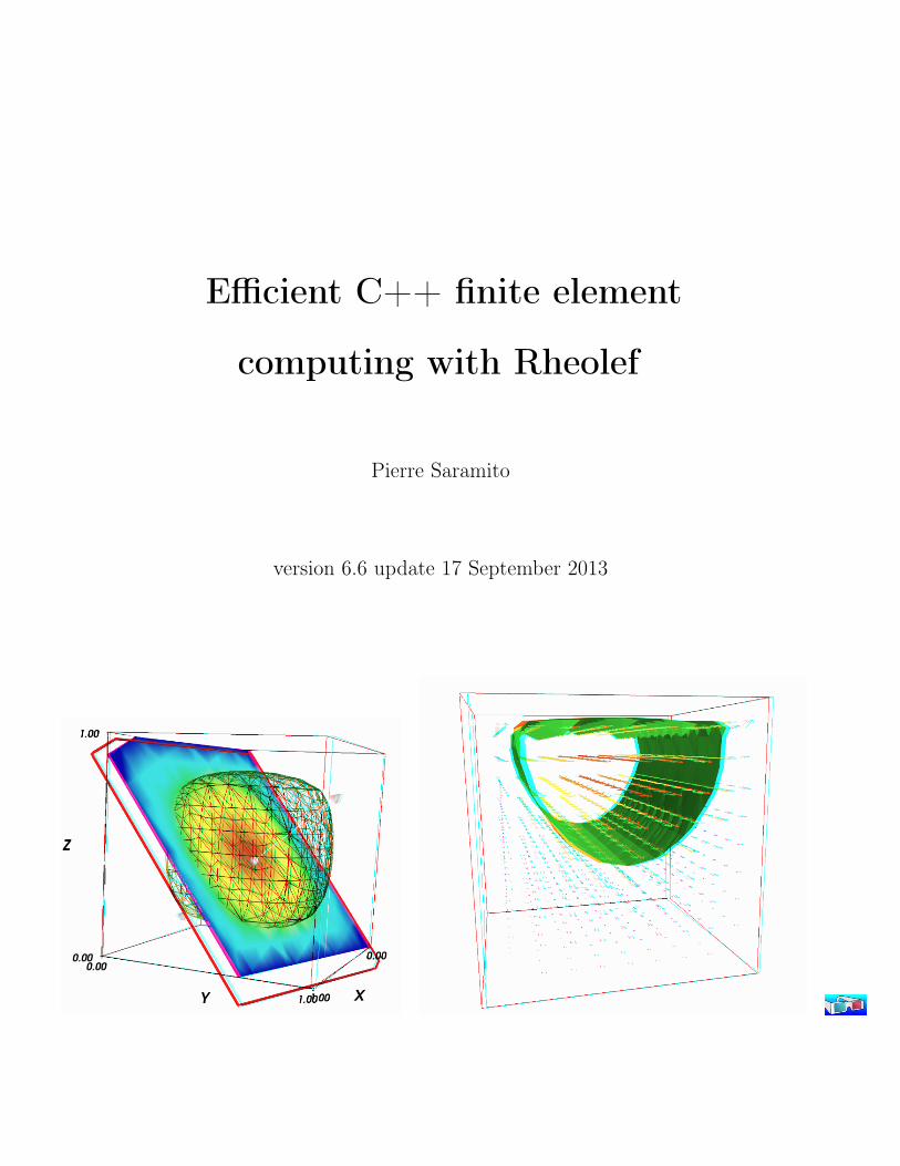
Efficient C++ finite element
computing with Rheolef
Pierre Saramito
version 6.6 update 17 September 2013

Copyright (c) 2003-2013 Pierre SaramitoPermission is granted to copy, distribute and/or modify this document under the terms of theGNU Free Documentation License, Version 1.3 or any later version published by the Free SoftwareFoundation; with no Invariant Sections, no Front-Cover Texts, and no Back-Cover Texts. A copyof the license is included in the section entitled "GNU Free Documentation License".

2 Rheolef version 6.6 update 17 September 2013
Introduction
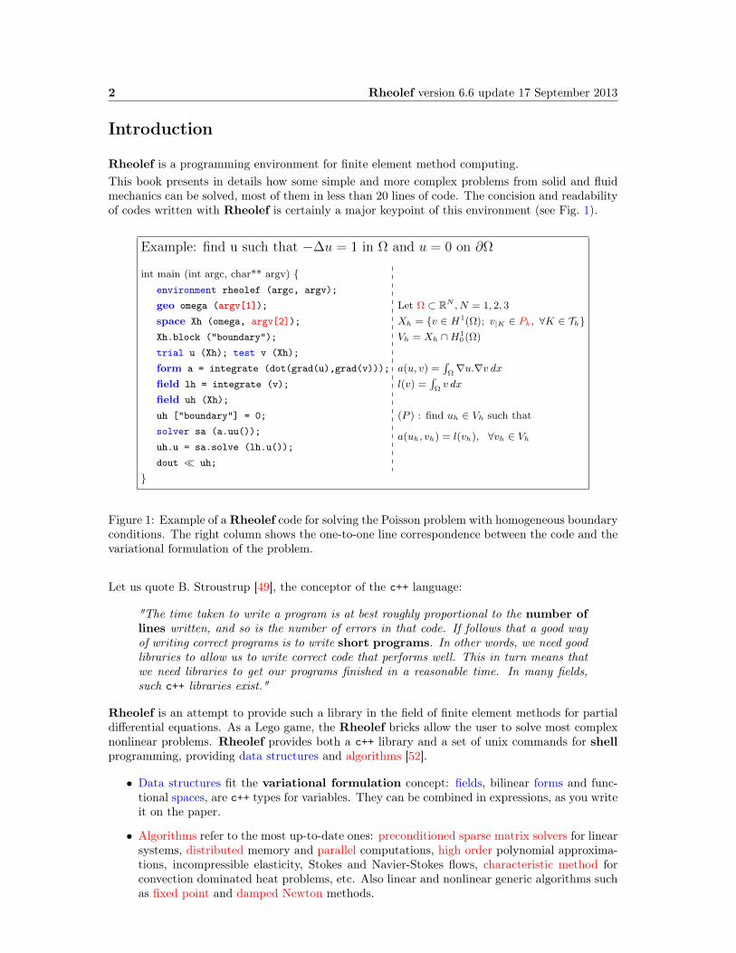
Rheolef is a programming environment for finite element method computing.This book presents in details how some simple and more complex problems from solid and fluidmechanics can be solved, most of them in less than 20 lines of code. The concision and readabilityof codes written with Rheolef is certainly a major keypoint of this environment (see Fig. 1).
Xh.block ("boundary");
space Xh (omega, argv[2]);
geo omega (argv[1]);
environment rheolef (argc, argv);
int main (int argc, char** argv)
field uh (Xh);
uh ["boundary"] = 0;
solver sa (a.uu());
uh.u = sa.solve (lh.u());
dout ≪ uh;
field lh = integrate (v);
form a = integrate (dot(grad(u),grad(v)));
trial u (Xh); test v (Xh);
Example: find u such that −∆u = 1 in Ω and u = 0 on ∂Ω
Let Ω ⊂ RN , N = 1, 2, 3
Xh = v ∈ H1(Ω); v|K ∈ Pk, ∀K ∈ ThVh = Xh ∩H1
0 (Ω)
a(u, v) =∫Ω∇u.∇v dx
l(v) =∫Ωv dx
(P ) : find uh ∈ Vh such that
a(uh, vh) = l(vh), ∀vh ∈ Vh
Figure 1: Example of aRheolef code for solving the Poisson problem with homogeneous boundaryconditions. The right column shows the one-to-one line correspondence between the code and thevariational formulation of the problem.
Let us quote B. Stroustrup [49], the conceptor of the c++ language:
"The time taken to write a program is at best roughly proportional to the number oflines written, and so is the number of errors in that code. If follows that a good wayof writing correct programs is to write short programs. In other words, we need goodlibraries to allow us to write correct code that performs well. This in turn means thatwe need libraries to get our programs finished in a reasonable time. In many fields,such c++ libraries exist."
Rheolef is an attempt to provide such a library in the field of finite element methods for partialdifferential equations. As a Lego game, the Rheolef bricks allow the user to solve most complexnonlinear problems. Rheolef provides both a c++ library and a set of unix commands for shellprogramming, providing data structures and algorithms [52].
• Data structures fit the variational formulation concept: fields, bilinear forms and func-tional spaces, are c++ types for variables. They can be combined in expressions, as you writeit on the paper.
• Algorithms refer to the most up-to-date ones: preconditioned sparse matrix solvers for linearsystems, distributed memory and parallel computations, high order polynomial approxima-tions, incompressible elasticity, Stokes and Navier-Stokes flows, characteristic method forconvection dominated heat problems, etc. Also linear and nonlinear generic algorithms suchas fixed point and damped Newton methods.

Rheolef version 6.6 update 17 September 2013 3
An efficient usage of Rheolef supposes a raisonable knowledge of the c++ programming language(see e.g. [43, 48]) and also of the classical finite element method and its variational principles.

4 Rheolef version 6.6 update 17 September 2013
Contacts
email [email protected]
home page http://www-ljk.imag.fr/membres/Pierre.Saramito/rheolef
Please send all comments and bug reports by electronic mail to
The Rheolef present contributorsfrom 2008 Ibrahim Cheddadi: discontinuous Galerkin method for transport problems.from 2010 Mahamar Dicko: finite element methods for equations on surfaces.from 2002 Jocelyn Étienne: characteristic method for time-dependent problems.from 2000 Pierre Saramito: project leader: main developments and code maintainer.
Past contributors2010 Lara Abouorm: banded level set method for equations on surfaces.2000 Nicolas Roquet: initial versions of Stokes and Bingham flow solvers.
Contents
Notations 8
I Getting started with simple problems 11
1 Getting started with Rheolef 151.1 The model problem . . . . . . . . . . . . . . . . . . . . . . . . . . . . . . . . . . . . 151.2 Approximation . . . . . . . . . . . . . . . . . . . . . . . . . . . . . . . . . . . . . . 161.3 Comments . . . . . . . . . . . . . . . . . . . . . . . . . . . . . . . . . . . . . . . . . 161.4 How to compile the code . . . . . . . . . . . . . . . . . . . . . . . . . . . . . . . . . 181.5 How to run the program . . . . . . . . . . . . . . . . . . . . . . . . . . . . . . . . . 191.6 Distributed and parallel runs . . . . . . . . . . . . . . . . . . . . . . . . . . . . . . 191.7 Stereo visualization . . . . . . . . . . . . . . . . . . . . . . . . . . . . . . . . . . . . 201.8 High-order finite element methods . . . . . . . . . . . . . . . . . . . . . . . . . . . 211.9 Tridimensional computations . . . . . . . . . . . . . . . . . . . . . . . . . . . . . . 211.10 Quadrangles, prisms and hexahedra . . . . . . . . . . . . . . . . . . . . . . . . . . 22
2 Standard boundary conditions 232.1 Non-homogeneous Dirichlet conditions . . . . . . . . . . . . . . . . . . . . . . . . . 232.2 Non-homogeneous Neumann boundary conditions for the Helmholtz operator . . . 312.3 The Robin boundary conditions . . . . . . . . . . . . . . . . . . . . . . . . . . . . . 332.4 Neumann boundary conditions for the Laplace operator . . . . . . . . . . . . . . . 35
3 Non-constant coefficients and multi-regions 39
II Fluids and solids computations 45
4 The linear elasticity and the Stokes problems 474.1 The linear elasticity problem . . . . . . . . . . . . . . . . . . . . . . . . . . . . . . 474.2 Computing the stress tensor . . . . . . . . . . . . . . . . . . . . . . . . . . . . . . . 514.3 Mesh adaptation . . . . . . . . . . . . . . . . . . . . . . . . . . . . . . . . . . . . . 544.4 The Stokes problem . . . . . . . . . . . . . . . . . . . . . . . . . . . . . . . . . . . 574.5 Computing the vorticity . . . . . . . . . . . . . . . . . . . . . . . . . . . . . . . . . 604.6 Computing the stream function . . . . . . . . . . . . . . . . . . . . . . . . . . . . . 62
5 Nearly incompressible elasticity and the stabilized Stokes problems 65
5
6 Rheolef version 6.6 update 17 September 2013
5.1 The incompressible elasticity problem . . . . . . . . . . . . . . . . . . . . . . . . . 655.2 The P1b− P1 element for the Stokes problem . . . . . . . . . . . . . . . . . . . . . 675.3 Axisymmetric geometries . . . . . . . . . . . . . . . . . . . . . . . . . . . . . . . . 735.4 The axisymmetric stream function and stress tensor . . . . . . . . . . . . . . . . . 73
6 Time-dependent problems 776.1 The heat equation . . . . . . . . . . . . . . . . . . . . . . . . . . . . . . . . . . . . 776.2 The convection-diffusion problem . . . . . . . . . . . . . . . . . . . . . . . . . . . . 806.3 The Navier-Stokes problem . . . . . . . . . . . . . . . . . . . . . . . . . . . . . . . 86
III Advanced and highly nonlinear problems 95
7 Equation defined on a surface 977.1 Approximation on an explicit surface mesh . . . . . . . . . . . . . . . . . . . . . . 977.2 Building a surface mesh from a level set function . . . . . . . . . . . . . . . . . . . 1067.3 The banded level set method . . . . . . . . . . . . . . . . . . . . . . . . . . . . . . 1097.4 A direct solver for the banded level set method . . . . . . . . . . . . . . . . . . . . 111
8 The highly nonlinear p-laplacian problem 1178.1 Problem statement . . . . . . . . . . . . . . . . . . . . . . . . . . . . . . . . . . . . 1178.2 The fixed-point algorithm . . . . . . . . . . . . . . . . . . . . . . . . . . . . . . . . 1188.3 The Newton algorithm . . . . . . . . . . . . . . . . . . . . . . . . . . . . . . . . . . 1268.4 The damped Newton algorithm . . . . . . . . . . . . . . . . . . . . . . . . . . . . . 1328.5 Error analysis . . . . . . . . . . . . . . . . . . . . . . . . . . . . . . . . . . . . . . . 135
IV Technical appendices 139
A How to write a variational formulation ? 141A.1 The Green formula . . . . . . . . . . . . . . . . . . . . . . . . . . . . . . . . . . . . 141A.2 The vectorial Green formula . . . . . . . . . . . . . . . . . . . . . . . . . . . . . . . 141A.3 The Green formula on a surface . . . . . . . . . . . . . . . . . . . . . . . . . . . . . 142
B How to prepare a mesh ? 143B.1 Bidimensional mesh with bamg . . . . . . . . . . . . . . . . . . . . . . . . . . . . . 143B.2 Unidimensional mesh with gmsh . . . . . . . . . . . . . . . . . . . . . . . . . . . . . 144B.3 Bidimensional mesh with gmsh . . . . . . . . . . . . . . . . . . . . . . . . . . . . . 145B.4 Tridimensional mesh with gmsh . . . . . . . . . . . . . . . . . . . . . . . . . . . . . 146
C Migrating to Rheolef version 6.0 149C.1 What is new in Rheolef 6.0 ? . . . . . . . . . . . . . . . . . . . . . . . . . . . . . . 149C.2 What should I have to change in my 5.x code ? . . . . . . . . . . . . . . . . . . . . 149C.3 New features in Rheolef 6.4 . . . . . . . . . . . . . . . . . . . . . . . . . . . . . . 151
D GNU Free Documentation License 153
List of example files 161

Rheolef version 6.6 update 17 September 2013 7
List of commands 163
Index 164
8 Rheolef version 6.6 update 17 September 2013
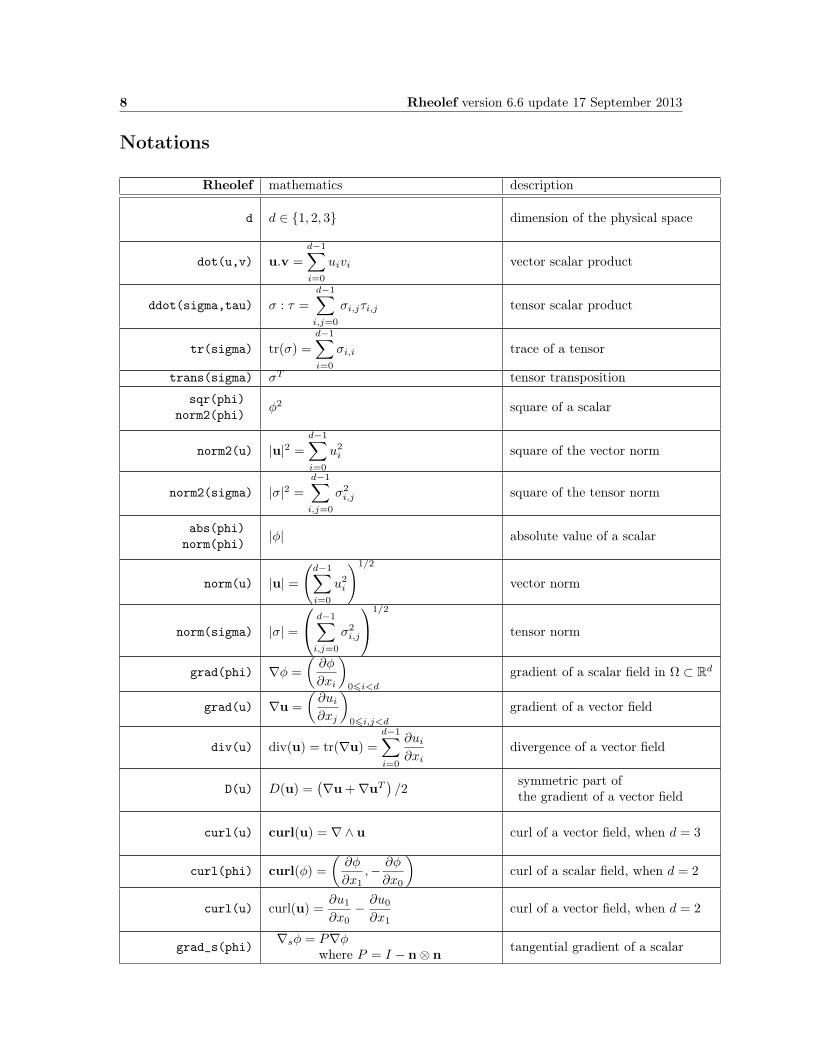
Notations
Rheolef mathematics description
d d ∈ 1, 2, 3 dimension of the physical space
dot(u,v) u.v =
d−1∑
i=0
uivi vector scalar product
ddot(sigma,tau) σ : τ =
d−1∑
i,j=0
σi,jτi,j tensor scalar product
tr(sigma) tr(σ) =
d−1∑
i=0
σi,i trace of a tensor
trans(sigma) σT tensor transposition
sqr(phi)norm2(phi) φ2 square of a scalar
norm2(u) |u|2 =
d−1∑
i=0
u2i square of the vector norm
norm2(sigma) |σ|2 =
d−1∑
i,j=0
σ2i,j square of the tensor norm
abs(phi)norm(phi) |φ| absolute value of a scalar
norm(u) |u| =(d−1∑
i=0
u2i
)1/2
vector norm
norm(sigma) |σ| =
d−1∑
i,j=0
σ2i,j
1/2
tensor norm
grad(phi) ∇φ =
(∂φ
∂xi
)
06i<d
gradient of a scalar field in Ω ⊂ Rd
grad(u) ∇u =
(∂ui∂xj
)
06i,j<d
gradient of a vector field
div(u) div(u) = tr(∇u) =
d−1∑
i=0
∂ui∂xi
divergence of a vector field
D(u) D(u) =(∇u +∇uT
)/2
symmetric part ofthe gradient of a vector field
curl(u) curl(u) = ∇∧ u curl of a vector field, when d = 3
curl(phi) curl(φ) =
(∂φ
∂x1,− ∂φ
∂x0
)curl of a scalar field, when d = 2
curl(u) curl(u) =∂u1
∂x0− ∂u0
∂x1curl of a vector field, when d = 2
grad_s(phi)∇sφ = P∇φ
where P = I − n⊗ ntangential gradient of a scalar
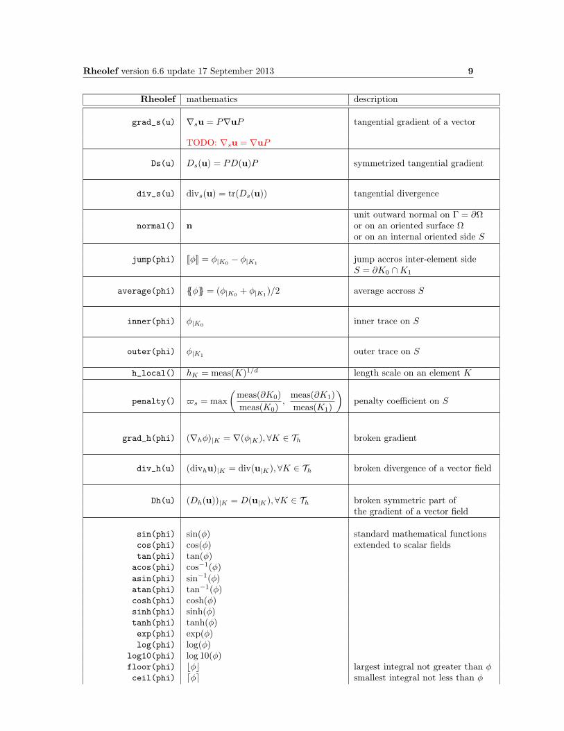
Rheolef version 6.6 update 17 September 2013 9
Rheolef mathematics description
grad_s(u) ∇su = P∇uP tangential gradient of a vector
TODO: ∇su = ∇uP
Ds(u) Ds(u) = PD(u)P symmetrized tangential gradient
div_s(u) divs(u) = tr(Ds(u)) tangential divergence
unit outward normal on Γ = ∂Ωnormal() n or on an oriented surface Ω
or on an internal oriented side S
jump(phi) [[φ]] = φ|K0− φ|K1
jump accros inter-element sideS = ∂K0 ∩K1
average(phi) φ = (φ|K0+ φ|K1
)/2 average accross S
inner(phi) φ|K0inner trace on S
outer(phi) φ|K1outer trace on S
h_local() hK = meas(K)1/d length scale on an element K
penalty() $s = max
(meas(∂K0)
meas(K0),
meas(∂K1)
meas(K1)
)penalty coefficient on S
grad_h(phi) (∇hφ)|K = ∇(φ|K),∀K ∈ Th broken gradient
div_h(u) (divhu)|K = div(u|K),∀K ∈ Th broken divergence of a vector field
Dh(u) (Dh(u))|K = D(u|K),∀K ∈ Th broken symmetric part ofthe gradient of a vector field
sin(phi) sin(φ) standard mathematical functionscos(phi) cos(φ) extended to scalar fieldstan(phi) tan(φ)acos(phi) cos−1(φ)asin(phi) sin−1(φ)atan(phi) tan−1(φ)cosh(phi) cosh(φ)sinh(phi) sinh(φ)tanh(phi) tanh(φ)exp(phi) exp(φ)log(phi) log(φ)
log10(phi) log 10(φ)floor(phi) bφc largest integral not greater than φceil(phi) dφe smallest integral not less than φ
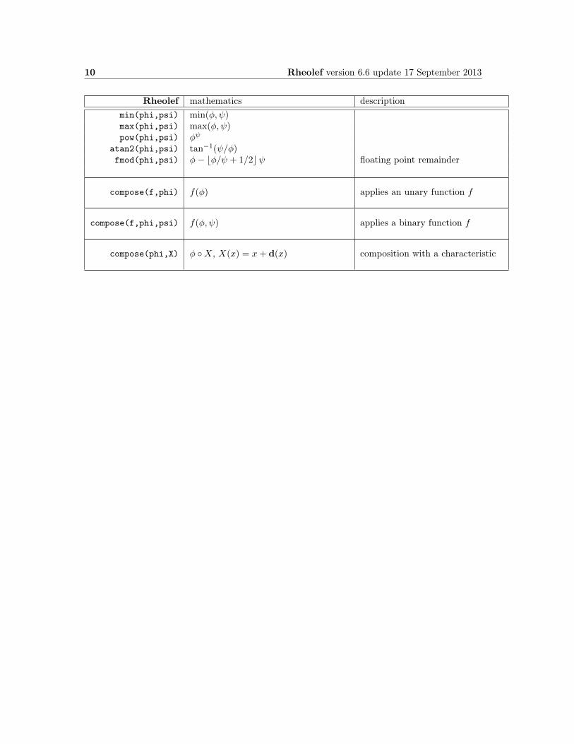
10 Rheolef version 6.6 update 17 September 2013
Rheolef mathematics descriptionmin(phi,psi) min(φ, ψ)max(phi,psi) max(φ, ψ)pow(phi,psi) φψ
atan2(phi,psi) tan−1(ψ/φ)fmod(phi,psi) φ− bφ/ψ + 1/2cψ floating point remainder
compose(f,phi) f(φ) applies an unary function f
compose(f,phi,psi) f(φ, ψ) applies a binary function f
compose(phi,X) φ X, X(x) = x+ d(x) composition with a characteristic
Part I
Getting started with simpleproblems
11


Rheolef version 6.6 update 17 September 2013 13
The first part of this book starts with the Dirichlet problem with homogeneous boundary condition:this example is declined with details in dimension 1, 2 and 3, as a starting point to Rheolef.Next chapters present various boundary conditions: for completeness, we treat non-homogeneousDirichlet, Neumann, and Robin boundary conditions for model problems. The last two examplespresents some special difficulties that appears in most problems: the first one introduce to problemswith non-constant coefficients and the second one, a ill-posed problem where the solution is definedup to a constant.This first part can be viewed as a pedagogic preparation for more advanced applications, such asStokes and elasticity, that are treated in the second part of this book. Problem with non-constantcoefficients are common as suproblems generated by various algorithms for non-linear problem.

14 Rheolef version 6.6 update 17 September 2013

Chapter 1
Getting started with Rheolef
For obtaining and installing Rheolef, see the installation instructions on the Rheolef home page:
http://www-ljk.imag.fr/membres/Pierre.Saramito/rheolef/
Before to run examples, please check your Rheolef installation with:
rheolef-config --check
The present book is available in the documentation directory of the Rheolef distribution. Thisdocumentation directory is given by the following unix command:
rheolef-config --docdir
All examples presented along the present book are also available in the example/ directory of theRheolef distribution. This directory is given by the following unix command:
rheolef-config --exampledir
This command returns you a path, something like /usr/share/doc/rheolef-doc/examples/ andyou should make a copy of these files:
cp -a /usr/share/doc/rheolef-doc/examples/ .cd examples
1.1 The model problem
Let us consider the classical Poisson problem with homogeneous Dirichlet boundary conditions ina domain bounded Ω ⊂ Rd, d = 1, 2, 3:(P): find u, defined in Ω, such that:
−∆u = 1 in Ω (1.1)u = 0 on ∂Ω (1.2)
where ∆ denotes the Laplace operator. The variational formulation of this problem expresses (seeappendix A.1 for details):(VF): find u ∈ H1
0 (Ω) such that:
a(u, v) = l(v), ∀v ∈ H10 (Ω) (1.3)
15
16 Rheolef version 6.6 update 17 September 2013
where the bilinear form a(., .) and the linear form l(.) are defined by
a(u, v) =
∫
Ω
∇u.∇v dx, ∀u, v ∈ H10 (Ω)
l(v) =
∫
Ω
v dx, ∀v ∈ L2(Ω)
The bilinear form a(., .) defines a scalar product in H10 (Ω) and is related to the energy form. This
form is associated to the −∆ operator.
1.2 Approximation
Let us introduce a mesh Th of Ω and the finite dimensional space Xh of continuous piecewisepolynomial functions.
Xh = v ∈ H1(Ω); v/K ∈ Pk, ∀K ∈ Th
where k = 1 or 2. Let Vh = Xh ∩H10 (Ω) be the functions of Xh that vanishes on the boundary of
Ω. The approximate problem expresses:(V F )h: find uh ∈ Vh such that:
a(uh, vh) = l(vh), ∀vh ∈ Vh
By developing uh on a basis of Vh, this problem reduces to a linear system. The following C++code implement this problem in the Rheolef environment.
Example file 1.1: dirichlet.cc1 #include "rheolef.h"2 using namespace rheolef;3 using namespace std;4 int main(int argc , char**argv) 5 environment rheolef (argc , argv);6 geo omega (argv [1]);7 space Xh (omega , argv [2]);8 Xh.block ("boundary");9 trial u (Xh); test v (Xh);
10 form a = integrate (dot(grad(u),grad(v)));11 field lh = integrate (v);12 field uh (Xh);13 uh ["boundary"] = 0;14 solver sa (a.uu());15 uh.set_u () = sa.solve (lh.u() - a.ub()*uh.b());16 dout << uh;17
1.3 Comments
This code applies for both one, two or three dimensional meshes and for both piecewise linear orquadratic finite element approximations. Four major classes are involved, namely: geo, space,form and field.Let us now comment the code, line by line.
#include "rheolef.h"
The first line includes the Rheolef header file ‘rheolef.h’.
using namespace rheolef;using namespace std;
Rheolef version 6.6 update 17 September 2013 17
By default, in order to avoid possible name conflicts when using another library, all class andfunction names are prefixed by rheolef::, as in rheolef::space. This feature is called the namespace. Here, since there is no possible conflict, and in order to simplify the syntax, we drop all therheolef:: prefixes, and do the same with the standard c++ library classes and variables, that arealso prefixed by std::.
int main(int argc , char**argv)
The entry function of the program is always called main and accepts arguments from the unixcommand line: argc is the counter of command line arguments and argv is the table of values.The character string argv[0] is the program name and argv[i], for i = 1 to argc-1, are theadditional command line arguments.
environment rheolef (argc , argv);
These two command line parameters are immediately furnished to the distributed environmentinitializer of the boost::mpi library, that is a c++ library based on the usual message passinginterface (mpi) library. Notice that this initialization is required, even when you run with onlyone processor.
geo omega (argv [1]);
This command get the first unix command-line argument argv[1] as a mesh file name and storethe corresponding mesh in the variable omega.
space Xh (omega , argv [2]);
Build the finite element space Xh contains all the piecewise polynomial continuous functions. Thepolynomial type is the second command-line arguments argv[2], and could be either P1, P2 orany Pk, where k > 1.
Xh.block ("boundary");
The homogeneous Dirichlet conditions are declared on the boundary.
trial u (Xh); test v (Xh);form a = integrate (dot(grad(u),grad(v)));
The bilinear form a(., .) is the energy form: it is defined for all functions u and v in Xh.
field lh = integrate (v);
The linear form lh(.) is associated to the constant right-hand side f = 1 of the problem. It isdefined for all v in Xh.
field uh (Xh);
The field uh contains the the degrees of freedom.
uh ["boundary"] = 0;
Some degrees of freedom are prescribed as zero on the boundary.Let (ϕi)06i<dim(Xh) be the basis of Xh associated to the Lagrange nodes, e.g. the vertices ofthe mesh for the P1 approximation and the vertices and the middle of the edges for the P2
approximation. The approximate solution uh expresses as a linear combination of the continuouspiecewise polynomial functions (ϕi):
uh =∑
i
uiϕi
Thus, the field uh is completely represented by its coefficients (ui). The coefficients (ui) of thiscombination are grouped into to sets: some have zero values, from the boundary condition andare related to blocked coefficients, and some others are unknown. Blocked coefficients are stored
18 Rheolef version 6.6 update 17 September 2013
into the uh.b array while unknown one are stored into uh.u. Thus, the restriction of the bilinearform a(., .) to Xh ×Xh can be conveniently represented by a block-matrix structure:
a(uh, vh) =(vh.u vh.b
)( a.uu a.uba.bu a.bb
)(uh.uuh.b
)
This representation also applies for the linear form l(.):
l(vh) =(vh.u vh.b
)( lh.ulh.b
)
Thus, the problem (V F )h writes now:
(vh.u vh.b
)( a.uu a.uba.bu a.bb
)(uh.uuh.b
)=(vh.u vh.b
)( lh.ulh.b
)
for any vh.u and where vh.b = 0. After expansion, the problem reduces to find uh.u such that:
a.uu ∗ uh.u = l.u− a.ub ∗ uh.b
The resolution of this linear system for the a.uu matrix is then performed. A preliminary stepbuild the LDLT factorization:
solver sa (a.uu());
Then, the second step solves the unknown part:
uh.set_u () = sa.solve (lh.u() - a.ub()*uh.b());
When d > 3, a faster iterative strategy is automatically preferred by the solver class for solvingthe linear system: in that case, the preliminary step build an incomplete Choleski factorizationpreconditioner, while the second step runs an iterative method: the preconditioned conjugategradient algorithm. Finally, the field is printed to standard output:
dout << uh;
The dout stream is a specific variable defined in the Rheolef library: it is a distributed andparallel extension of the usual cout stream in C++
1.4 How to compile the code
First, create a file ‘Makefile’ as follow:
include $(shell rheolef-config --libdir)/rheolef/rheolef.mkCXXFLAGS = $(INCLUDES_RHEOLEF)LDLIBS = $(LIBS_RHEOLEF)default: dirichlet
Then, enter:
make dirichlet
Now, your program, linked with Rheolef, is ready to run on a mesh.

Rheolef version 6.6 update 17 September 2013 19
1.5 How to run the program
Figure 1.1: Solution of the model problem for d = 2: (left) P1 element; (right) P2 element.
Enter the commands:
mkgeo_grid -t 10 > square.geogeo square.geo
The first command generates a simple 10x10 bidimensional mesh of Ω =]0, 1[2 and stores it in thefile square.geo. The second command shows the mesh. It uses gnuplot visualization programby default.The next command performs the computation:
./dirichlet square.geo P1 > square.fieldfield square.field
1.6 Distributed and parallel runs
Alternatively, a computation in a distributed and parallel environment writes:
mpirun -np 4 ./dirichlet square.geo P1 > square.field

20 Rheolef version 6.6 update 17 September 2013
Figure 1.2: Alternative representations of the solution of the model problem (d = 2 and the P1
element): (left) in black-and-white; (right) in elevation and stereoscopic anaglyph mode.
1.7 Stereo visualization
Also explore some graphic rendering modes (see Fig. 1.2):
field square.field -bwfield square.field -grayfield square.field -mayavifield square.field -elevation -nofill -stereo
The last command shows the solution in elevation and in stereoscopic anaglyph mode (see Fig. 1.4,left). The anaglyph mode requires red-cyan glasses: red for the left eye and cyan for the right one,as shown on Fig. 1.3.
Figure 1.3: Red-cyan anaglyph glasses for the stereoscopic visualization.
In the book, stereo figures are indicated by the logo in the right margin. See http://en.wikipedia.org/wiki/Anaglyph_image for more and http://www.alpes-stereo.com/

Rheolef version 6.6 update 17 September 2013 21
lunettes.html for how to find anaglyph red-cyan glasses. Please, consults the correspondingunix manual page for more on field, geo and mkgeo_grid:
man mkgeo_gridman geoman field
1.8 High-order finite element methods
Turning to the P2 or P3 approximations simply writes:
./dirichlet square.geo P2 > square-P2.fieldfield square-P2.field
Fig. 1.1.right shows the result. You can replace the P2 command-line argument by any Pk, wherek > 1. Now, let us consider a mono-dimensional problem Ω =]0, 1[:
mkgeo_grid -e 10 > line.geogeo line.geo./dirichlet line.geo P1 | field -
The first command generates a subdivision containing ten edge elements. The last two lines showthe mesh and the solution via gnuplot visualization, respectively.Conversely, the P2 case writes:
./dirichlet line.geo P2 | field -
1.9 Tridimensional computations
Let us consider a three-dimensional problem Ω =]0, 1[3. First, let us generate a mesh:
mkgeo_grid -T 10 > cube.geogeo cube.geogeo cube.geo -stereo -fullgeo cube.geo -stereo -cut
The previous commands draw the mesh with all internal edges (-full), stereoscopic anaglyph(-stereo)and then with a cut (-cut) inside the internal structure: a simple click on the centralarrow draws the cut plane normal vector or its origin, while the red square allows a translation.
22 Rheolef version 6.6 update 17 September 2013
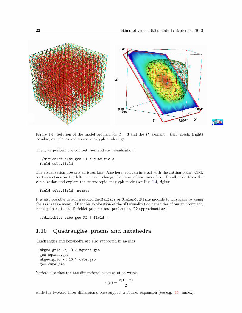
Figure 1.4: Solution of the model problem for d = 3 and the P1 element : (left) mesh; (right)isovalue, cut planes and stereo anaglyph renderings.
Then, we perform the computation and the visualization:
./dirichlet cube.geo P1 > cube.fieldfield cube.field
The visualization presents an isosurface. Also here, you can interact with the cutting plane. Clickon IsoSurface in the left menu and change the value of the isosurface. Finally exit from thevisualization and explore the stereoscopic anaglyph mode (see Fig. 1.4, right):
field cube.field -stereo
It is also possible to add a second IsoSurface or ScalarCutPlane module to this scene by usingthe Visualize menu. After this exploration of the 3D visualization capacities of our environment,let us go back to the Dirichlet problem and perform the P2 approximation:
./dirichlet cube.geo P2 | field -
1.10 Quadrangles, prisms and hexahedra
Quadrangles and hexahedra are also supported in meshes:
mkgeo_grid -q 10 > square.geogeo square.geomkgeo_grid -H 10 > cube.geogeo cube.geo
Notices also that the one-dimensional exact solution writes:
u(x) =x(1− x)
2
while the two-and three dimensional ones support a Fourier expansion (see e.g. [45], annex).

Chapter 2
Standard boundary conditions
We show how to deal with various non-homogeneous boundary conditions of Dirichlet, Neumanand Robin type.
2.1 Non-homogeneous Dirichlet conditions
Formulation
We turn now to the case of a non-homogeneous Dirichlet boundary conditions. Let f ∈ H−1(Ω)
and g ∈ H 12 (∂Ω). The problem writes:
(P2) find u, defined in Ω such that:
−∆u = f in Ω
u = g on ∂Ω
The variational formulation of this problem expresses:(V F2) find u ∈ V such that:
a(u, v) = l(v), ∀v ∈ V0
where
a(u, v) =
∫
Ω
∇u.∇v dx
l(v) =
∫
Ω
f v dx
V = v ∈ H1(Ω); v|∂Ω = gV0 = H1
0 (Ω)
Approximation
As usual, we introduce a mesh Th of Ω and the finite dimensional space Xh:
Xh = v ∈ H1(Ω); v/K ∈ Pk, ∀K ∈ Th
Then, we introduce:
Vh = v ∈ Xh; v|∂Ω = πh(g)V0,h = v ∈ Xh; v|∂Ω = 0
23

24 Rheolef version 6.6 update 17 September 2013
where πh denotes the Lagrange interpolation operator. The approximate problem writes:(V F2)h: find uh ∈ Vh such that:
a(uh, vh) = l(vh), ∀vh ∈ V0,h
The following C++ code implement this problem in the Rheolef environment.
Example file 2.1: dirichlet-nh.cc1 #include "rheolef.h"2 using namespace rheolef;3 using namespace std;4 #include "cosinusprod_laplace.icc"5 int main(int argc , char**argv) 6 environment rheolef(argc , argv);7 geo omega (argv [1]);8 size_t d = omega.dimension ();9 space Xh (omega , argv [2]);
10 Xh.block ("boundary");11 trial u (Xh); test v (Xh);12 form a = integrate (dot(grad(u),grad(v)));13 field lh = integrate (f(d)*v);14 field uh (Xh);15 space Wh (omega["boundary"], argv [2]);16 uh ["boundary"] = interpolate(Wh , g(d));17 solver sa (a.uu());18 uh.set_u () = sa.solve (lh.u() - a.ub()*uh.b());19 dout << uh;20
Let us choose Ω ⊂ Rd, d = 1, 2, 3 with
f(x) = d π2d−1∏
i=0
cos(πxi) and g(x) =
d−1∏
i=0
cos(πxi) (2.1)
Remarks the notation x = (x0, . . . , xd−1) for the Cartesian coordinates in Rd: since all arraysstart at index zero in C++ codes, and in order to avoid any mistakes between the code and themathematical formulation, we also adopt this convention here. This choice of f and g is convenient,since the exact solution is known:
u(x) =
d−1∏
i=0
cos(πxi)
The following C++ code implement this problem by using the concept of function object, alsocalled class-function (see e.g. [29]). A convenient feature is the ability for function objects to storeauxiliary parameters, such as the space dimension d for f here, or some constants, as π for f andg.
Example file 2.2: cosinusprod_laplace.icc1 struct f : field_functor <f,Float > 2 Float operator () (const point& x) const 3 return d*pi*pi*cos(pi*x[0])* cos(pi*x[1])* cos(pi*x[2]); 4 f(size_t d1) : d(d1), pi(acos(Float ( -1))) 5 size_t d; const Float pi;6 ;7 struct g : field_functor <g,Float > 8 Float operator () (const point& x) const 9 return cos(pi*x[0])* cos(pi*x[1])* cos(pi*x[2]);
10 g(size_t d1) : pi(acos(Float (-1))) 11 const Float pi;12 ;
Rheolef version 6.6 update 17 September 2013 25
Comments
The class point describes the coordinates of a point (x0, . . . , xd−1) ∈ Rd as a d-uplet of Float.The Float type is usually a double. This type depends upon the Rheolef configuration (see [42],installation instructions), and could also represent some high precision floating point class. Thedirichlet-nh.cc code looks like the previous one dirichlet.cc related to homogeneous bound-ary conditions. Let us comments the changes. The dimension d comes from the geometry Ω:
size_t d = omega.dimension ();
The linear form l(.) is associated to the right-hand side f and writes:field lh = integrate (f(d)*v);
Notice that the function object f is build with the dimension d as parameter. Notice also the useof field_functor1in the definition of the class f: this trick allows us to mixt functions, fields andtest-functions in the same expression, as f(d) ∗ v.The space Wh of piecewise Pk functions defined on the boundary ∂Ω is defined by:
space Wh (omega["boundary"], argv [2]);
where Pk is defined via the second command line argument argv[2]. This space is suitable forthe Lagrange interpolation of g on the boundary:
uh ["boundary"] = interpolate(Wh , g(d));
The values of the degrees of freedom related to the boundary are stored into the field uh.b, wherenon-homogeneous Dirichlet conditions applies. The rest of the code is similar to the homogeneousDirichlet case.
2.1.1 How to run the program
First, compile the program:
make dirichlet-nh
Running the program is obtained from the homogeneous Dirichlet case, by replacing dirichletby dirichlet-nh:
mkgeo_grid -e 10 > line.geo./dirichlet-nh line.geo P1 > line.fieldfield line.field
for the bidimensional case:
mkgeo_grid -t 10 > square.geo./dirichlet-nh square.geo P1 > square.fieldfield square.field
and for the tridimensional case:
mkgeo_grid -T 10 > box.geo./dirichlet-nh box.geo P1 > box.fieldfield -mayavi box.field
Here, the P1 approximation can be replaced by P2, P3, etc, by modifying the command-lineargument.
1The actual implementation of a field_functor class bases on the curiously recurring template pattern (CRTP)C++ idiom: the definition of the class f derives from field_functor<f,Float> that depend itself upon f. So,be carrefull when using copy-paste, as there a no checks if you write e.g. field_functor<g,Float> with anotherfunction g instead of f.

26 Rheolef version 6.6 update 17 September 2013
2.1.2 Error analysis
Principle
Since the solution u is regular, the following error estimates holds:
‖u− uh‖0,2,Ω ≈ O(hk+1)
‖u− uh‖0,∞,Ω ≈ O(hk+1)
‖u− uh‖1,2,Ω ≈ O(hk)
providing the approximate solution uh uses Pk continuous finite element method, k > 1. Here,‖.‖0,2,Ω, ‖.‖0,∞,Ω and ‖.‖1,2,Ω denotes as usual the L2(Ω), L∞(Ω) and H1(Ω) norms.By denoting πh the Lagrange interpolation operator, the triangular inequality leads to:
‖u− uh‖0,2,Ω 6 ‖(I − πh)(u)‖0,2,Ω + ‖uh − πhu‖0,2,Ω
From the fundamental properties of the Laplace interpolation πh, and since u is smooth enough,we have ‖(I−πh)(u)‖0,2,Ω ≈ O(hk+1). Thus, we have just to check the ‖uh−πhu‖0,2,Ω term. Thefollowing code implement the computation of the error.
Example file 2.3: cosinusprod_error.cc1 #include "rheolef.h"2 using namespace rheolef;3 using namespace std;4 #include "cosinusprod.icc"5 int main(int argc , char**argv) 6 environment rheolef(argc , argv);7 Float error_linf_expected = (argc > 1) ? atof(argv [1]) : 1e+38;8 field uh; din >> uh;9 space Xh = uh.get_space ();
10 size_t d = Xh.get_geo (). dimension ();11 field pi_h_u = interpolate(Xh, u_exact(d));12 field eh = uh - pi_h_u;13 trial u (Xh); test v (Xh);14 form m = integrate (u*v);15 form a = integrate (dot(grad(u),grad(v)));16 dout << "error_l2 " << sqrt(m(eh,eh)) << endl17 << "error_linf " << eh.max_abs () << endl18 << "error_h1 " << sqrt(a(eh ,eh)) << endl;19 return (eh.max_abs () <= error_linf_expected) ? 0 : 1;20
Example file 2.4: cosinusprod.icc1 struct u_exact : field_functor <u_exact ,Float > 2 Float operator () (const point& x) const 3 return cos(pi*x[0])* cos(pi*x[1])* cos(pi*x[2]); 4 u_exact(size_t d1) : d(d1), pi(acos(Float ( -1.0))) 5 size_t d; Float pi;6 ;
The m(., .) is here the classical scalar product on L2(Ω), and is related to the mass form.
Running the program
make dirichlet-nh cosinusprod_error
After compilation, run the code by using the command:
mkgeo_grid -t 10 > square.geo./dirichlet-nh square.geo P1 | ./cosinusprod_error
Rheolef version 6.6 update 17 September 2013 27
10−10
10−8
10−6
10−4
10−2
10−2 10−1
h
‖uh − πh(u)‖0,2,Ω
2 = k + 1
3
4 k = 1k = 2k = 3
10−10
10−8
10−6
10−4
10−2
10−2 10−1
h
‖uh − πh(u)‖0,∞,Ω
2 = k + 1
3
4
k = 1k = 2k = 3
10−8
10−6
10−4
10−2
100
10−2 10−1
h
|uh − πh(u)|1,2,Ω
1 = k
2
3
k = 1k = 2k = 3
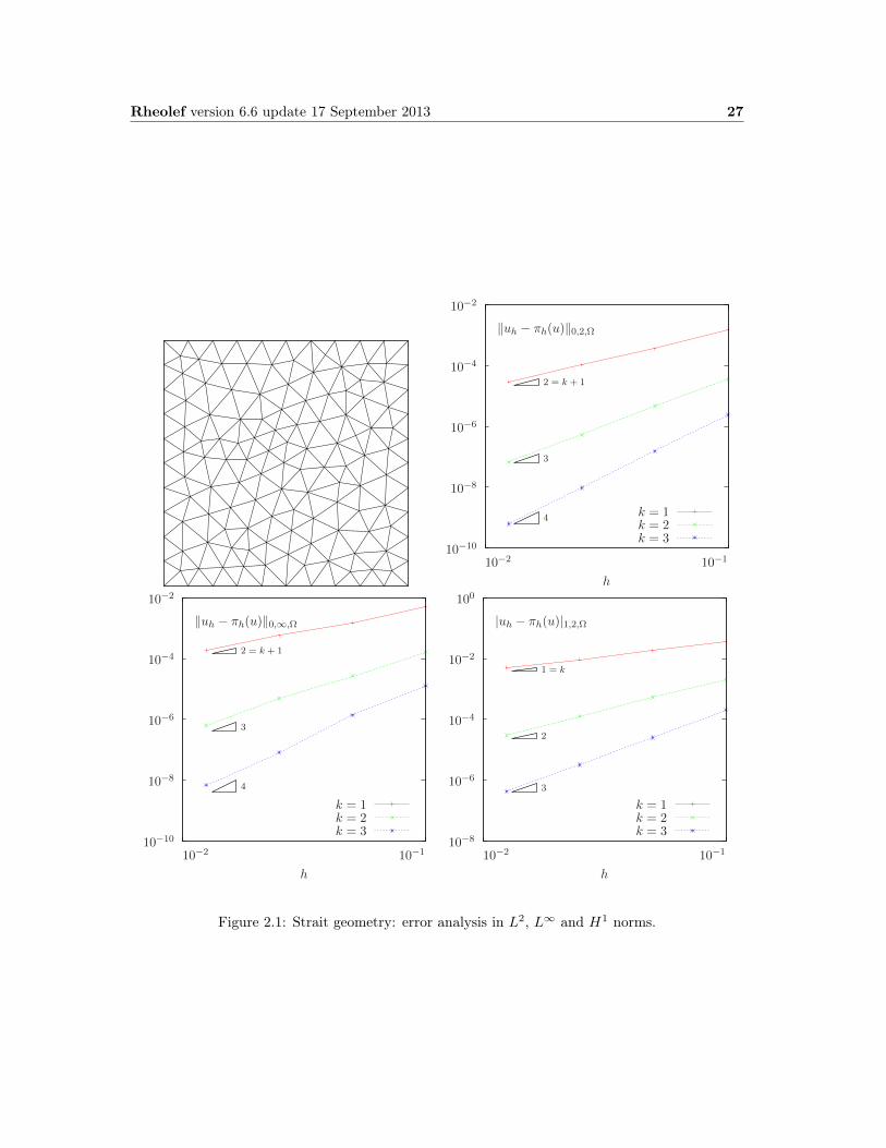
Figure 2.1: Strait geometry: error analysis in L2, L∞ and H1 norms.
28 Rheolef version 6.6 update 17 September 2013
The three L2, L∞ and H1 errors are printed for a h = 1/10 uniform mesh. Note that an unstruc-tured quasi-uniform mesh can be simply generated by using the mkgeo_ugrid command:
mkgeo_ugrid -t 10 > square.geogeo square.geo
Let nel denotes the number of elements in the mesh. Since the mesh is quasi-uniform, we haveh ≈ n
1d
el where d is the physical space dimension. Here d = 2 for our bidimensional mesh. Figure 2.1
plots in logarithmic scale the error versus n12
el for both Pk approximations, k = 1, 2, 3 and thevarious norms. Observe that the error behaves as predicted by the theory.
Curved domains
The error analysis applies also for curved boundaries and high order approximations.
Example file 2.5: cosinusrad_laplace.icc1 struct f : field_functor <f,Float > 2 Float operator () (const point& x) const 3 Float r = sqrt(sqr(x[0])+ sqr(x[1])+ sqr(x[2]));4 Float sin_over_ar = (r == 0) ? 1 : sin(a*r)/(a*r);5 return sqr(a)*((d-1)* sin_over_ar + cos(a*r)); 6 f(size_t d1) : d(d1), a(acos(Float ( -1.0))) 7 size_t d; Float a;8 ;9 struct g : field_functor <g,Float >
10 Float operator () (const point& x) const 11 return cos(a*sqrt(sqr(x[0])+ sqr(x[1])+ sqr(x[2]))); 12 g(size_t =0) : a(acos(Float ( -1.0))) 13 Float a;14 ;
Example file 2.6: cosinusrad.icc1 struct u_exact : field_functor <u_exact ,Float > 2 Float operator () (const point& x) const 3 Float r = sqrt(sqr(x[0])+ sqr(x[1])+ sqr(x[2]));4 return cos(a*r); 5 u_exact(size_t =0) : a(acos(Float ( -1.0))) 6 Float a;7 ;
First, generate the test source file and compile it:
sed -e ’s/sinusprod/sinusrad/’ < dirichlet-nh.cc > dirichlet_nh_ball.ccsed -e ’s/sinusprod/sinusrad/’ < cosinusprod_error.cc > cosinusrad_error.ccmake dirichlet_nh_ball cosinusrad_error
Then, generates the mesh of a circle and run the test case:
mkgeo_ball -order 1 -t 10 > circle-P1.geogeo circle-P1./dirichlet_nh_ball circle-P1.geo P1 | ./cosinusrad_error
For a high order k = 3 isoparametric approximation:
mkgeo_ball -order 3 -t 10 > circle-P3.geogeo circle-P3./dirichlet_nh_ball circle-P3.geo P3 | ./cosinusrad_error
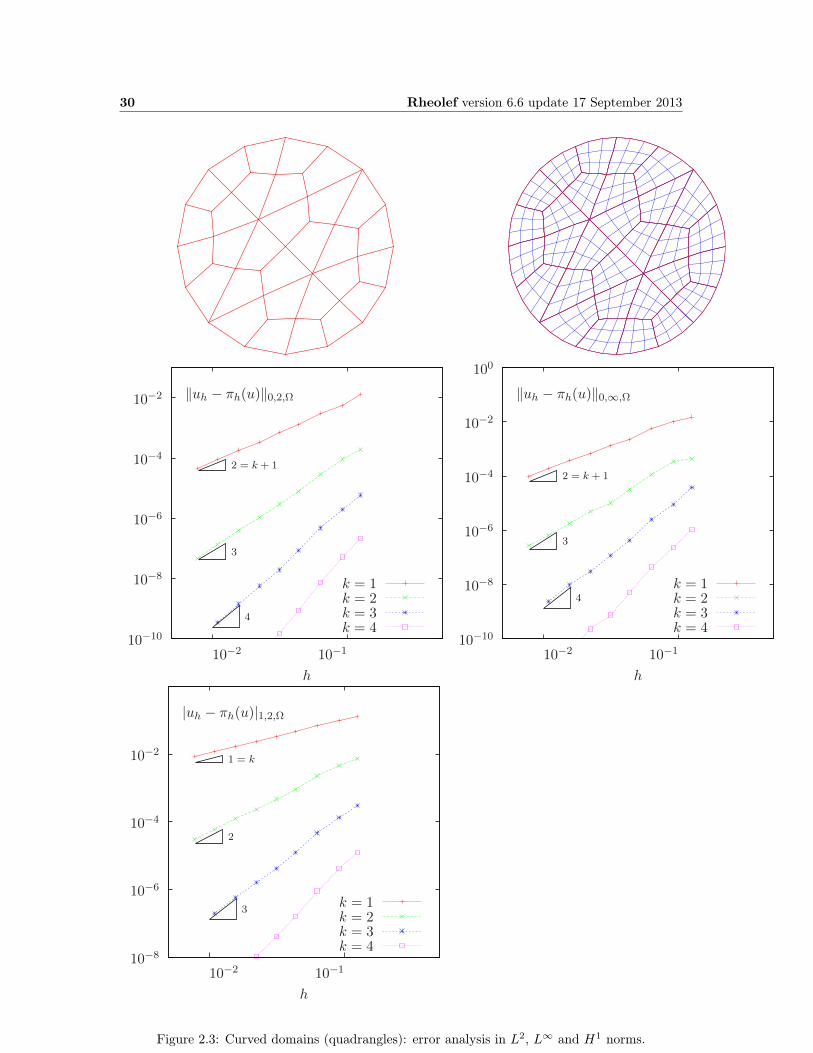
Observe Fig. 2.2: for meshes based on triangles: the error behave as expected when k = 1, 2, 3, 4.A similar result occurs for quadrangles, as shown on Fig. 2.3.

Rheolef version 6.6 update 17 September 2013 29
10−10
10−8
10−6
10−4
10−2
100
10−2 10−1
h
‖uh − πh(u)‖0,2,Ω
2 = k + 1
3
4
k = 1k = 2k = 3k = 4
10−10
10−8
10−6
10−4
10−2
100
10−2 10−1
h
‖uh − πh(u)‖0,∞,Ω
2 = k + 1
3
4k = 1k = 2k = 3k = 4
10−8
10−6
10−4
10−2
100
10−2 10−1
h
|uh − πh(u)|1,2,Ω
1 = k
2
3
k = 1k = 2k = 3k = 4
Figure 2.2: Curved domains (triangles): error analysis in L2, L∞ and H1 norms.
30 Rheolef version 6.6 update 17 September 2013
10−10
10−8
10−6
10−4
10−2
10−2 10−1
h
‖uh − πh(u)‖0,2,Ω
2 = k + 1
3
4
k = 1k = 2k = 3k = 4
10−10
10−8
10−6
10−4
10−2
100
10−2 10−1
h
‖uh − πh(u)‖0,∞,Ω
2 = k + 1
3
4k = 1k = 2k = 3k = 4
10−8
10−6
10−4
10−2
10−2 10−1
h
|uh − πh(u)|1,2,Ω
1 = k
2
3k = 1k = 2k = 3k = 4
Figure 2.3: Curved domains (quadrangles): error analysis in L2, L∞ and H1 norms.
Rheolef version 6.6 update 17 September 2013 31
mkgeo_ball -order 3 -q 10 > circle-q-P3.geogeo circle-q-P3./dirichlet_nh_ball circle-q-P3.geo P3 | ./cosinusrad_error
These features are currently in development for arbitrarily Pk high order approximations andthree-dimensional geometries.
2.2 Non-homogeneous Neumann boundary conditions forthe Helmholtz operator
Formulation
Let us show how to insert Neumann boundary conditions. Let f ∈ H−1(Ω) and g ∈ H− 12 (∂Ω).
The problem writes:(P3): find u, defined in Ω such that:
u−∆u = f in Ω
∂u
∂n= g on ∂Ω
The variational formulation of this problem expresses:(V F3): find u ∈ H1(Ω) such that:
a(u, v) = l(v), ∀v ∈ H1(Ω)
where
a(u, v) =
∫
Ω
(u v +∇u.∇v) dx
l(v) =
∫
Ω
f v dx+
∫
∂Ω
g v ds
32 Rheolef version 6.6 update 17 September 2013
Approximation
As usual, we introduce a mesh Th of Ω and the finite dimensional space Xh:
Xh = v ∈ H1(Ω); v/K ∈ Pk, ∀K ∈ Th
The approximate problem writes:(V F3)h: find uh ∈ Xh such that:
a(uh, vh) = l(vh), ∀vh ∈ Xh
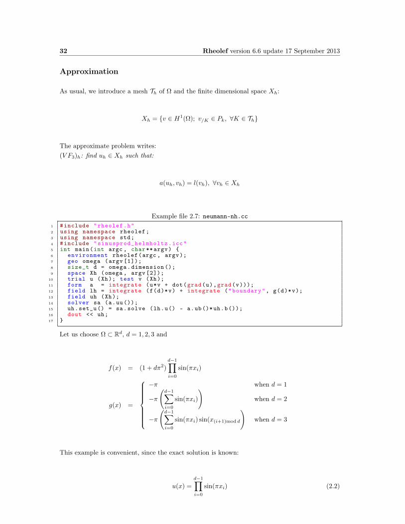
Example file 2.7: neumann-nh.cc1 #include "rheolef.h"2 using namespace rheolef;3 using namespace std;4 #include "sinusprod_helmholtz.icc"5 int main(int argc , char**argv) 6 environment rheolef(argc , argv);7 geo omega (argv [1]);8 size_t d = omega.dimension ();9 space Xh (omega , argv [2]);
10 trial u (Xh); test v (Xh);11 form a = integrate (u*v + dot(grad(u),grad(v)));12 field lh = integrate (f(d)*v) + integrate ("boundary", g(d)*v);13 field uh (Xh);14 solver sa (a.uu());15 uh.set_u () = sa.solve (lh.u() - a.ub()*uh.b());16 dout << uh;17
Let us choose Ω ⊂ Rd, d = 1, 2, 3 and
f(x) = (1 + dπ2)
d−1∏
i=0
sin(πxi)
g(x) =
−π when d = 1
−π(d−1∑
i=0
sin(πxi)
)when d = 2
−π(d−1∑
i=0
sin(πxi) sin(x(i+1)mod d
)when d = 3
This example is convenient, since the exact solution is known:
u(x) =
d−1∏
i=0
sin(πxi) (2.2)

Rheolef version 6.6 update 17 September 2013 33
Example file 2.8: sinusprod_helmholtz.icc1 struct f : field_functor <f,Float > 2 Float operator () (const point& x) const 3 switch (d) 4 case 1: return (1+d*pi*pi)*sin(pi*x[0]);5 case 2: return (1+d*pi*pi)*sin(pi*x[0])* sin(pi*x[1]);6 default: return (1+d*pi*pi)*sin(pi*x[0])* sin(pi*x[1])* sin(pi*x[2]);7 8 f(size_t d1) : d(d1), pi(acos(Float ( -1.0))) 9 size_t d; const Float pi;
10 ;11 struct g : field_functor <g,Float > 12 Float operator () (const point& x) const 13 switch (d) 14 case 1: return -pi;15 case 2: return -pi*(sin(pi*x[0]) + sin(pi*x[1]));16 default: return -pi*( sin(pi*x[0])* sin(pi*x[1])17 + sin(pi*x[1])* sin(pi*x[2])18 + sin(pi*x[2])* sin(pi*x[0]));19 20 g(size_t d1) : d(d1), pi(acos(Float ( -1.0))) 21 size_t d; const Float pi;22 ;
Comments
The neumann-nh.cc code looks like the previous one dirichlet-nh.cc. Let us comments onlythe changes.
form a = integrate (u*v + dot(grad(u),grad(v)));
The bilinear form a(., .) is defined. Notes the flexibility of the integrate function that takes asargument an expression involving the trial and test functions. The right-hand side is computedas:
field lh = integrate (f(d)*v) + integrate ("boundary", g(d)*v);
The second integration is perfomed on ∂Ω. The additional first argument of the integratefunction is here the name of the integration domain.
2.2.1 How to run the program
First, compile the program:
make neumann-nh
Running the program is obtained from the homogeneous Dirichlet case, by replacing dirichletby neumann-nh.
2.3 The Robin boundary conditions
Formulation
Let f ∈ H−1(Ω) and Let g ∈ H 12 (∂Ω). The problem writes:
(P4) find u, defined in Ω such that:
−∆u = f in Ω
∂u
∂n+ u = g on ∂Ω

34 Rheolef version 6.6 update 17 September 2013
The variational formulation of this problem expresses:(V F4): find u ∈ H1(Ω) such that:
a(u, v) = l(v), ∀v ∈ H1(Ω)
where
a(u, v) =
∫
Ω
∇u.∇v dx+
∫
∂Ω
uv ds
l(v) =
∫
Ω
uv dx+
∫
∂Ω
gv ds
Approximation
As usual, letXh = v ∈ H1(Ω); v/K ∈ Pk, ∀K ∈ Th
The approximate problem writes:(V F4)h: find uh ∈ Xh such that:
a(uh, vh) = l(vh), ∀vh ∈ Xh
Example file 2.9: robin.cc1 #include "rheolef.h"2 using namespace rheolef;3 using namespace std;4 #include "cosinusprod_laplace.icc"5 int main(int argc , char**argv) 6 environment rheolef(argc , argv);7 geo omega (argv [1]);8 size_t d = omega.dimension ();9 space Xh (omega , argv [2]);
10 trial u (Xh); test v (Xh);11 form a = integrate (dot(grad(u),grad(v))) + integrate ("boundary", u*v);12 field lh = integrate (f(d)*v) + integrate ("boundary", g(d)*v);13 field uh (Xh);14 solver sa (a.uu());15 uh.set_u () = sa.solve (lh.u() - a.ub()*uh.b());16 dout << uh;17
Comments
The code robin.cc looks like the previous one neumann-nh.cc. Let us comments the changes.form a = integrate (dot(grad(u),grad(v))) + integrate ("boundary", u*v);
This statement reflects directly the definition of the bilinear form a(., .), as the sum of two integrals,the first one over Ω and the second one over its boundary.
2.3.1 How to run the program
First, compile the program:
make robin
Running the program is obtained from the homogeneous Dirichlet case, by replacing dirichletby robin.
Rheolef version 6.6 update 17 September 2013 35
2.4 Neumann boundary conditions for the Laplace operator
In this chapter we study how to solve a ill-posed problem with a solution defined up to a constant.
Formulation
Let Ω be a bounded open and simply connected subset of Rd, d = 1, 2 or 3. Let f ∈ L2(Ω) andg ∈ H 1
2 (∂Ω) satisfying the following compatibility condition:∫
Ω
f dx+
∫
∂Ω
g ds = 0
The problem writes:(P5)h: find u, defined in Ω such that:
−∆u = f in Ω
∂u
∂n= g on ∂Ω
Since this problem only involves the derivatives of u, it is clear that its solution is never unique [19,p. 11]. A discrete version of this problem could be solved iteratively by the conjugate gradientor the MINRES algorithm [34]. In order to solve it by a direct method, we turn the difficulty byseeking u in the following space
V = v ∈ H1(Ω); b(v, 1) = 0where
b(v, µ) =
∫
Ω
v dx, ∀v ∈ L2(Ω),∀µ ∈ R
The variational formulation of this problem writes:(V F5): find u ∈ V such that:
a(u, v) = l(v), ∀v ∈ Vwhere
a(u, v) =
∫
Ω
∇u.∇v dx
l(v) = m(f, v) +mb(g, v)
m(f, v) =
∫
Ω
fv dx
mb(g, v) =
∫
∂Ω
gv ds
Since the direct discretization of the space V is not an obvious task, the constraint b(u, 1) = 0is enforced by a Lagrange multiplier λ ∈ R. Let us introduce the Lagrangian, defined for allv ∈ H1(Ω) and µ ∈ R by:
L(v, µ) =1
2a(v, v) + b(v, µ)− l(v)
The saddle point (u, λ) ∈ H1(Ω)×R of this Lagrangian is characterized as the unique solution of:
a(u, v) + b(v, λ) = l(v), ∀v ∈ H1(Ω)
b(u, µ) = 0, ∀µ ∈ R
It is clear that if (u, λ) is solution of this problem, then u ∈ V and u is a solution of (V F5).Conversely, let u ∈ V the solution of (V F5). Choosing v = v0 where v0(x) = 1, ∀x ∈ Ω leads toλmeas(Ω) = l(v0). From the definition of l(.) and the compatibility condition between the data fand g, we get λ = 0. Notice that the saddle point problem extends to the case when f and g doesnot satisfies the compatibility condition, and in that case λ = l(v0)/meas(Ω).
36 Rheolef version 6.6 update 17 September 2013
Approximation
As usual, we introduce a mesh Th of Ω and the finite dimensional space Xh:
Xh = v ∈ H1(Ω); v/K ∈ Pk, ∀K ∈ Th
The approximate problem writes:(V F5)h: find (uh, λh) ∈ Xh × R such that:
a(uh, v) + b(v, λh) = lh(v), ∀v ∈ Xh
b(uh, µ) = 0, ∀µ ∈ R
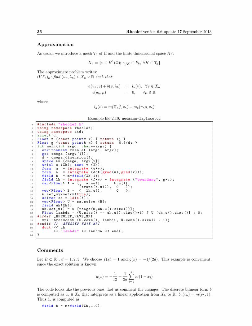
wherelh(v) = m(Πhf, vh) +mb(πhg, vh)
Example file 2.10: neumann-laplace.cc1 #include "rheolef.h"2 using namespace rheolef;3 using namespace std;4 size_t d;5 Float f (const point& x) return 1; 6 Float g (const point& x) return -0.5/d; 7 int main(int argc , char**argv) 8 environment rheolef (argc , argv);9 geo omega (argv [1]);
10 d = omega.dimension ();11 space Xh (omega , argv [2]);12 trial u (Xh); test v (Xh);13 form m = integrate (u*v);14 form a = integrate (dot(grad(u),grad(v)));15 field b = m*field(Xh ,1);16 field lh = integrate (f*v) + integrate ("boundary", g*v);17 csr <Float > A = a.uu(), b.u(),18 trans(b.u()), 0 ;19 vec <Float > B = lh.u(), 0 ;20 A.set_symmetry(true);21 solver sa = ldlt(A);22 vec <Float > U = sa.solve (B);23 field uh(Xh);24 uh.set_u () = U [range(0,uh.u(). size ())];25 Float lambda = (U.size() == uh.u(). size ()+1) ? U [uh.u(). size ()] : 0;26 #ifdef _RHEOLEF_HAVE_MPI27 mpi:: broadcast (U.comm(), lambda , U.comm (). size() - 1);28 #endif // _RHEOLEF_HAVE_MPI29 dout << uh30 << "lambda" << lambda << endl;31
Comments
Let Ω ⊂ Rd, d = 1, 2, 3. We choose f(x) = 1 and g(x) = −1/(2d). This example is convenient,since the exact solution is known:
u(x) = − 1
12+
1
2d
d∑
i=1
xi(1− xi)
The code looks like the previous ones. Let us comment the changes. The discrete bilinear form bis computed as bh ∈ Xh that interprets as a linear application from Xh to R: bh(vh) = m(vh, 1).Thus bh is computed as
field b = m*field(Xh ,1.0);

Rheolef version 6.6 update 17 September 2013 37
where the discrete bilinear form m is identified to its matrix and field(Xh,1.0) is the constantvector equal to 1. Let
A =
(a.uu trans(b.u)b.u 0
), U =
(uh.u
lambda
), B =
(lh.u
0
)
The problem admits the following matrix form:
A U = BThe matrix and right-hand side of the system are assembled by concatenation:csr <Float > A = a.uu , b.u,
trans(b.u), 0 ;vec <Float > B = lh.u, 0 ;
where csr and vec are respectively the matrix and vector classes. The csr is the abbreviation ofcompressed sparse row, a sparse matrix compression standard format. Notice that the matrix A issymmetric and non-singular, but indefinite : it admits eigenvalues that are either strictly positiveor strictly negative. While the Choleski factorization is not possible, its variant the LDLT one isperformed, thanks to the ldlt function:
solver sa = ldlt(A);
Then, the uh.u vector is extracted from the U one:uh.u = U [range(0,uh.u.size ())];
The extraction of lambda from U is more technical in a distributed environment. In a sequentialone, since it is stored after the uh.u values, it could be simply written as:
Float lambda = U [uh.u.size ()];
In a distributed environment, lambda is stored in U on the last processor, identified byU.comm().size()-1. Here U.comm() denotes the communicator, from the boost::mpi libraryand U.comm().size() is the number of processors in use, e.g. as specified by the mpirun com-mand. On this last processor, the array U has size equal to uh.u.size()+1 and lambda is storedin U[uh.u.size()]. On the others processors, the array U has size equal to uh.u.size() andlambda is not available. The following statement extract lambda on the last processor and set itto zero on the others:
Float lambda = (U.size() == uh.u.size ()+1) ? U [uh.u.size ()] : 0;
Then, the value of lambda is broadcasted on the others processors:mpi:: broadcast (U.comm(), lambda , U.comm (). size() - 1);
The preprocessing guards #idef. . .#endif assure that this example compile also when the libraryis not installed with the MPI support. Finally, the statement
dout << catchmark("u") << uh<< catchmark("lambda") << lambda << endl;
writes the solution (uh, λ). The catchmark function writes marks together with the solution inthe output stream. These marks are suitable for a future reading with the same format, as:
din >> catchmark("u") >> uh>> catchmark("lambda") >> lambda;
This is useful for post-treatment, visualization and error analysis.
2.4.1 How to run the program
As usual, enter:
make neumann-laplacemkgeo_grid -t 10 > square.geo./neumann-laplace square P1 | field -

38 Rheolef version 6.6 update 17 September 2013

Chapter 3
Non-constant coefficients andmulti-regions
This chapter is related to the so-called transmission problem. We introduce some new concepts:problems with non-constant coefficients, regions in the mesh, weighted forms and discontinuousapproximations.
Formulation
Let us consider a diffusion problem with a non-constant diffusion coefficient η in a domain boundedΩ ⊂ Rd, d = 1, 2, 3:(P ): find u defined in Ω such that:
−div(η∇u) = f in Ω (3.1)u = 0 on Γleft ∪ Γright (3.2)
∂u
∂n= 0 on Γtop ∪ Γbottom when d > 2 (3.3)
∂u
∂n= 0 on Γfront ∪ Γback when d = 3 (3.4)
where f is a given source term.
39

40 Rheolef version 6.6 update 17 September 2013
westeast
bottomrighttopleft
Figure 3.1: Transmission problem: the domain Ω partition: (Ωwest and Ωeast).
We consider here the important special case when η is piecewise constant:
η(x) =
ε when x ∈ Ωwest
1 when x ∈ Ωeast
where (Ωwest,Ωeast) is a partition of Ω in two parts (see Fig. 3.1). This is the so-called trans-mission problem: the solution and the flux are continuous on the interface Γ0 = ∂Ωeast ∩ ∂Ωwest
between the two domains where the problem reduce to a constant diffusion one:
uΩwest = uΩeast on Γ0
ε∂u/Ωwest
∂n=
∂uΩeast
∂non Γ0
It expresses the transmission of the quantity u and its flux across the interface Γ0 between tworegions that have different diffusion properties: Notice that the more classical problem, withconstant diffusion η on Ω is obtained by simply choosing when ε = 1.The variational formulation of this problem expresses:(V F ): find u ∈ V such that:
a(u, v) = l(v), ∀v ∈ V
where the bilinear forms a(., .) and the linear one l(.) are defined by
a(u, v) =
∫
Ω
η∇u.∇v dx, ∀u, v ∈ H1(Ω)
l(v) =
∫
Ω
f v dx, ∀v ∈ L2(Ω)
V = v ∈ H1(Ω); v = 0 on Γleft ∪ Γright
The bilinear form a(., .) defines a scalar product in V and is related to the energy form. This formis associated to the −div η∇ operator.The approximation of this problem could performed by a standard Lagrange Pk continuous ap-proximation.
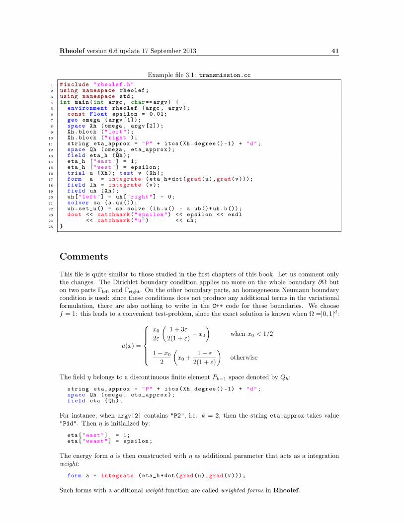
Rheolef version 6.6 update 17 September 2013 41
Example file 3.1: transmission.cc1 #include "rheolef.h"2 using namespace rheolef;3 using namespace std;4 int main(int argc , char**argv) 5 environment rheolef (argc , argv);6 const Float epsilon = 0.01;7 geo omega (argv [1]);8 space Xh (omega , argv [2]);9 Xh.block ("left");
10 Xh.block ("right");11 string eta_approx = "P" + itos(Xh.degree ()-1) + "d";12 space Qh (omega , eta_approx );13 field eta_h (Qh);14 eta_h ["east"] = 1;15 eta_h ["west"] = epsilon;16 trial u (Xh); test v (Xh);17 form a = integrate (eta_h*dot(grad(u),grad(v)));18 field lh = integrate (v);19 field uh (Xh);20 uh["left"] = uh["right"] = 0;21 solver sa (a.uu());22 uh.set_u () = sa.solve (lh.u() - a.ub()*uh.b());23 dout << catchmark("epsilon") << epsilon << endl24 << catchmark("u") << uh;25
Comments
This file is quite similar to those studied in the first chapters of this book. Let us comment onlythe changes. The Dirichlet boundary condition applies no more on the whole boundary ∂Ω buton two parts Γleft and Γright. On the other boundary parts, an homogeneous Neumann boundarycondition is used: since these conditions does not produce any additional terms in the variationalformulation, there are also nothing to write in the C++ code for these boundaries. We choosef = 1: this leads to a convenient test-problem, since the exact solution is known when Ω =]0, 1[d:
u(x) =
x0
2ε
(1 + 3ε
2(1 + ε)− x0
)when x0 < 1/2
1− x0
2
(x0 +
1− ε2(1 + ε)
)otherwise
The field η belongs to a discontinuous finite element Pk−1 space denoted by Qh:
string eta_approx = "P" + itos(Xh.degree ()-1) + "d";space Qh (omega , eta_approx );field eta (Qh);
For instance, when argv[2] contains "P2", i.e. k = 2, then the string eta_approx takes value"P1d". Then η is initialized by:
eta["east"] = 1;eta["weast"] = epsilon;
The energy form a is then constructed with η as additional parameter that acts as a integrationweight:
form a = integrate (eta_h*dot(grad(u),grad(v)));
Such forms with a additional weight function are called weighted forms in Rheolef.
42 Rheolef version 6.6 update 17 September 2013
How to run the program ?
Build the program as usual: make transmission. Then, creates a one-dimensional geometry withtwo regions:
mkgeo_grid -e 100 -region > line.geogeo line.geo
The trivial mesh generator mkgeo_grid, defines two regions east and west when used with the-region option. This correspond to the situation:
Ω = [0, 1]d, Ωwest = Ω ∩ x0 < 1/2 and Ωeast = Ω ∩ x0 > 1/2.
In order to avoid mistakes with the C++ style indexes, we denote by (x0, . . . , xd−1) the Cartesiancoordinate system in Rd.Finally, run the program and look at the solution:
make transmission./transmission line.geo P1 > line.fieldfield line.field
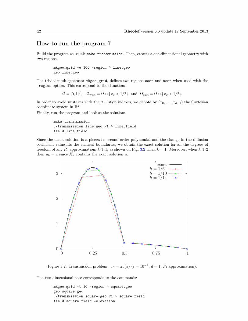
Since the exact solution is a piecewise second order polynomial and the change in the diffusioncoefficient value fits the element boundaries, we obtain the exact solution for all the degrees offreedom of any Pk approximation, k > 1, as shown on Fig. 3.2 when k = 1. Moreover, when k > 2then uh = u since Xh contains the exact solution u.
0
1
2
3
0 0.25 0.5 0.75 1
exacth = 1/6h = 1/10h = 1/14
Figure 3.2: Transmission problem: uh = πh(u) (ε = 10−2, d = 1, P1 approximation).
The two dimensional case corresponds to the commands:
mkgeo_grid -t 10 -region > square.geogeo square.geo./transmission square.geo P1 > square.fieldfield square.field -elevation

Rheolef version 6.6 update 17 September 2013 43
while the tridimensional to
mkgeo_grid -T 10 -region > cube.geo./transmission cube.geo P1 > cube.mfieldfield cube.field
As for all the others examples, you can replace P1 by higher-order approximations, change elementsshapes, such as q, H or P, and run distributed computations computations with mpirun.

44 Rheolef version 6.6 update 17 September 2013

Part II
Fluids and solids computations
45

Chapter 4
The linear elasticity and the Stokesproblems
4.1 The linear elasticity problem
Formulation
The total Cauchy stress tensor expresses:
σ(u) = λ div(u).I + 2µD(u) (4.1)
where λ and µ are the Lamé coefficients. Here, D(u) denotes the symmetric part of the gradi-ent operator and div is the divergence operator. Let us consider the elasticity problem for theembankment, in Ω =]0, 1[d, d = 2, 3. The problem writes:
(P ): find u = (u0, . . . , ud−1), defined in Ω, such that:
− div σ(u) = f in Ω,∂u
∂n= 0 on Γtop ∪ Γright
u = 0 on Γleft ∪ Γbottom,u = 0 on Γfront ∪ Γback, when d = 3
(4.2)
where f = (0,−1) when d = 2 and f = (0, 0,−1) when d = 3. The Lamé coefficients are assumedto satisfy µ > 0 and λ + µ > 0. Since the problem is linear, we can suppose that µ = 1 withoutany loss of generality.
47
48 Rheolef version 6.6 update 17 September 2013
x2
x1
left right
bottom
top
front
x1
x0bottom
rightleft
top
x0
back
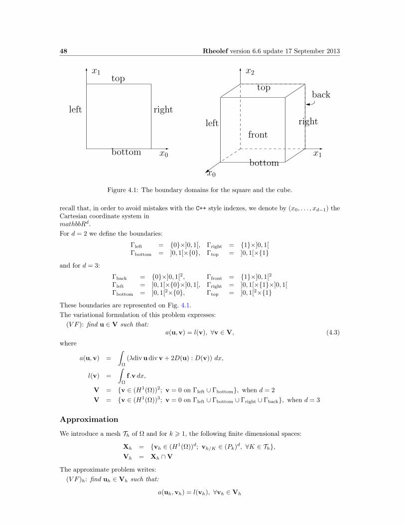
Figure 4.1: The boundary domains for the square and the cube.
recall that, in order to avoid mistakes with the C++ style indexes, we denote by (x0, . . . , xd−1) theCartesian coordinate system inmathbbRd.For d = 2 we define the boundaries:
Γleft = 0×]0, 1[, Γright = 1×]0, 1[Γbottom = ]0, 1[×0, Γtop = ]0, 1[×1
and for d = 3:
Γback = 0×]0, 1[2, Γfront = 1×]0, 1[2
Γleft = ]0, 1[×0×]0, 1[, Γright = ]0, 1[×1×]0, 1[Γbottom = ]0, 1[2×0, Γtop = ]0, 1[2×1
These boundaries are represented on Fig. 4.1.The variational formulation of this problem expresses:
(V F ): find u ∈ V such that:a(u,v) = l(v), ∀v ∈ V, (4.3)
where
a(u,v) =
∫
Ω
(λdivudivv + 2D(u) : D(v)) dx,
l(v) =
∫
Ω
f .v dx,
V = v ∈ (H1(Ω))2; v = 0 on Γleft ∪ Γbottom, when d = 2
V = v ∈ (H1(Ω))3; v = 0 on Γleft ∪ Γbottom ∪ Γright ∪ Γback, when d = 3
Approximation
We introduce a mesh Th of Ω and for k > 1, the following finite dimensional spaces:
Xh = vh ∈ (H1(Ω))d; vh/K ∈ (Pk)d, ∀K ∈ Th,Vh = Xh ∩V
The approximate problem writes:(V F )h: find uh ∈ Vh such that:
a(uh,vh) = l(vh), ∀vh ∈ Vh
Rheolef version 6.6 update 17 September 2013 49
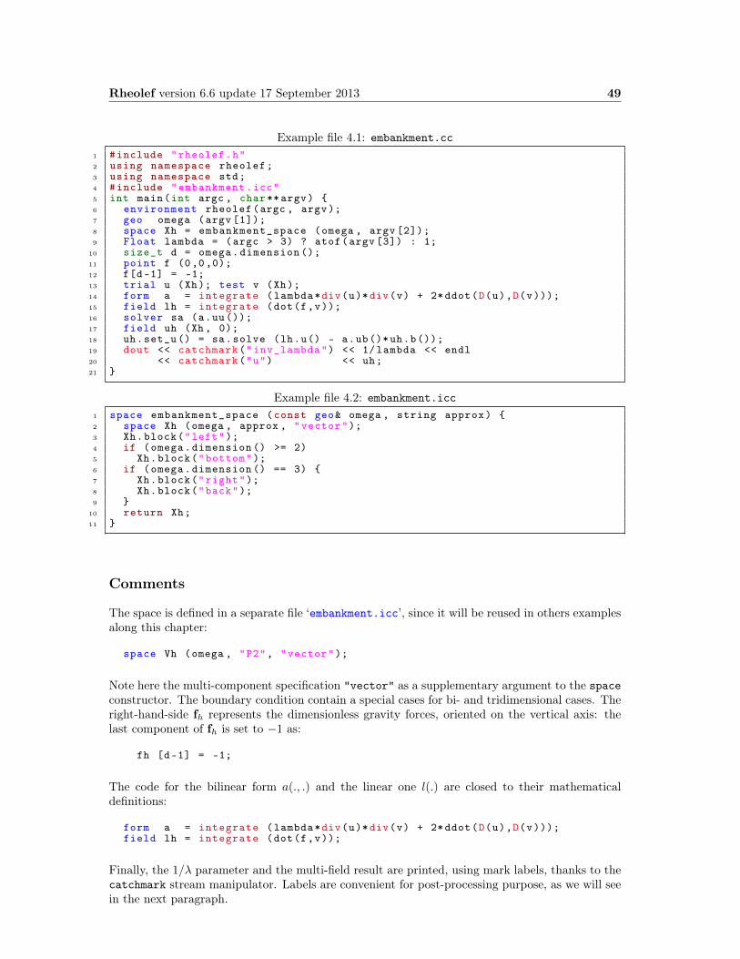
Example file 4.1: embankment.cc1 #include "rheolef.h"2 using namespace rheolef;3 using namespace std;4 #include "embankment.icc"5 int main(int argc , char**argv) 6 environment rheolef(argc , argv);7 geo omega (argv [1]);8 space Xh = embankment_space (omega , argv [2]);9 Float lambda = (argc > 3) ? atof(argv [3]) : 1;
10 size_t d = omega.dimension ();11 point f (0,0,0);12 f[d-1] = -1;13 trial u (Xh); test v (Xh);14 form a = integrate (lambda*div(u)*div(v) + 2*ddot(D(u),D(v)));15 field lh = integrate (dot(f,v));16 solver sa (a.uu());17 field uh (Xh, 0);18 uh.set_u () = sa.solve (lh.u() - a.ub()*uh.b());19 dout << catchmark("inv_lambda") << 1/ lambda << endl20 << catchmark("u") << uh;21
Example file 4.2: embankment.icc1 space embankment_space (const geo& omega , string approx) 2 space Xh (omega , approx , "vector");3 Xh.block("left");4 if (omega.dimension () >= 2)5 Xh.block("bottom");6 if (omega.dimension () == 3) 7 Xh.block("right");8 Xh.block("back");9
10 return Xh;11
Comments
The space is defined in a separate file ‘embankment.icc’, since it will be reused in others examplesalong this chapter:
space Vh (omega , "P2", "vector");
Note here the multi-component specification "vector" as a supplementary argument to the spaceconstructor. The boundary condition contain a special cases for bi- and tridimensional cases. Theright-hand-side fh represents the dimensionless gravity forces, oriented on the vertical axis: thelast component of fh is set to −1 as:
fh [d-1] = -1;
The code for the bilinear form a(., .) and the linear one l(.) are closed to their mathematicaldefinitions:
form a = integrate (lambda*div(u)*div(v) + 2*ddot(D(u),D(v)));field lh = integrate (dot(f,v));
Finally, the 1/λ parameter and the multi-field result are printed, using mark labels, thanks to thecatchmark stream manipulator. Labels are convenient for post-processing purpose, as we will seein the next paragraph.

50 Rheolef version 6.6 update 17 September 2013
How to run the program
Figure 4.2: The linear elasticity for λ = 1 and d = 2 and d = 3: both wireframe and filled surfaces; stereoscopic anaglyph mode for 3D solutions.
Compile the program as usual (see page 18):
make embankment
and enter the commands:
mkgeo_grid -t 10 > square.geogeo square.geo
The triangular mesh has four boundary domains, named left, right, top and bottom. Then,enter:
./embankment square.geo P1 > square-P1.field

Rheolef version 6.6 update 17 September 2013 51
The previous command solves the problem for the corresponding mesh and writes the multi-component solution in the ‘.field’ file format. Run the deformation vector field visualizationusing the default gnuplot render:
field square-P1.fieldfield square-P1.field -nofill
Note the graphic options usage ; the unix manual for the field command is available as:
man field
The view is shown on Fig. 4.2. A specific field component can be also selected for a scalarvisualization:
field -comp 0 square-P1.fieldfield -comp 1 square-P1.field
Next, perform a P2 approximation of the solution:
./embankment square.geo P2 > square-P2.fieldfield square-P2.field -mayavi -nofill
Finally, let us consider the three dimensional case
mkgeo_grid -T 10 > cube.geo./embankment cube.geo P1 > cube-P1.fieldfield cube-P1.field -stereofield cube-P1.field -stereo -fill
The two last commands show the solution in 3D stereoscopic anaglyph mode. The graphic isrepresented on Fig. 4.2. The P2 approximation writes:
./embankment cube.geo P2 > cube-P2.fieldfield cube-P2.field
4.2 Computing the stress tensor
Formulation and approximation
The following code computes the total Cauchy stress tensor, reading the Lamé coefficient λ andthe deformation field uh from a ‘.field’ file. Let us introduce:
Th = τh ∈ (L2(Ω))d×d; τh = τTh and τh;ij/K ∈ Pk−1, ∀K ∈ Th, 1 6 i, j 6 d
This computation expresses:find σh such that:
m(σh, τ) = b(τ,uh),∀τ ∈ Thwhere
m(σ, τ) =
∫
Ω
σ : τ dx,
b(τ,u) =
∫
Ω
(2D(u) : τ dx+ λdiv(u) tr(τ)) dx,
where tr(τ) =∑di=1 τii is the trace of the tensor τ .
52 Rheolef version 6.6 update 17 September 2013
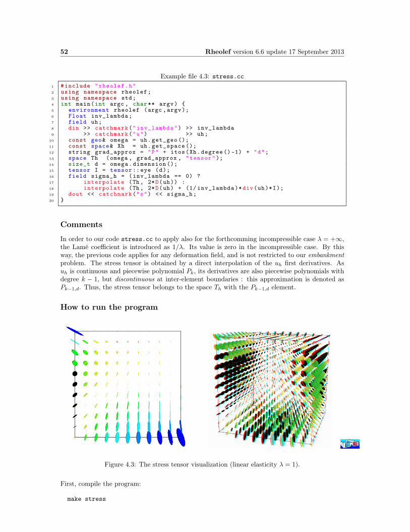
Example file 4.3: stress.cc1 #include "rheolef.h"2 using namespace rheolef;3 using namespace std;4 int main(int argc , char** argv) 5 environment rheolef (argc ,argv);6 Float inv_lambda;7 field uh;8 din >> catchmark("inv_lambda") >> inv_lambda9 >> catchmark("u") >> uh;
10 const geo& omega = uh.get_geo ();11 const space& Xh = uh.get_space ();12 string grad_approx = "P" + itos(Xh.degree ()-1) + "d";13 space Th (omega , grad_approx , "tensor");14 size_t d = omega.dimension ();15 tensor I = tensor ::eye (d);16 field sigma_h = (inv_lambda == 0) ?17 interpolate (Th, 2*D(uh)) :18 interpolate (Th, 2*D(uh) + (1/ inv_lambda )*div(uh)*I);19 dout << catchmark("s") << sigma_h;20
Comments
In order to our code stress.cc to apply also for the forthcomming incompressible case λ = +∞,the Lamé coefficient is introduced as 1/λ. Its value is zero in the incompressible case. By thisway, the previous code applies for any deformation field, and is not restricted to our embankmentproblem. The stress tensor is obtained by a direct interpolation of the uh first derivatives. Asuh is continuous and piecewise polynomial Pk, its derivatives are also piecewise polynomials withdegree k − 1, but discontinuous at inter-element boundaries : this approximation is denoted asPk−1,d. Thus, the stress tensor belongs to the space Th with the Pk−1,d element.
How to run the program
Figure 4.3: The stress tensor visualization (linear elasticity λ = 1).
First, compile the program:
make stress
Rheolef version 6.6 update 17 September 2013 53
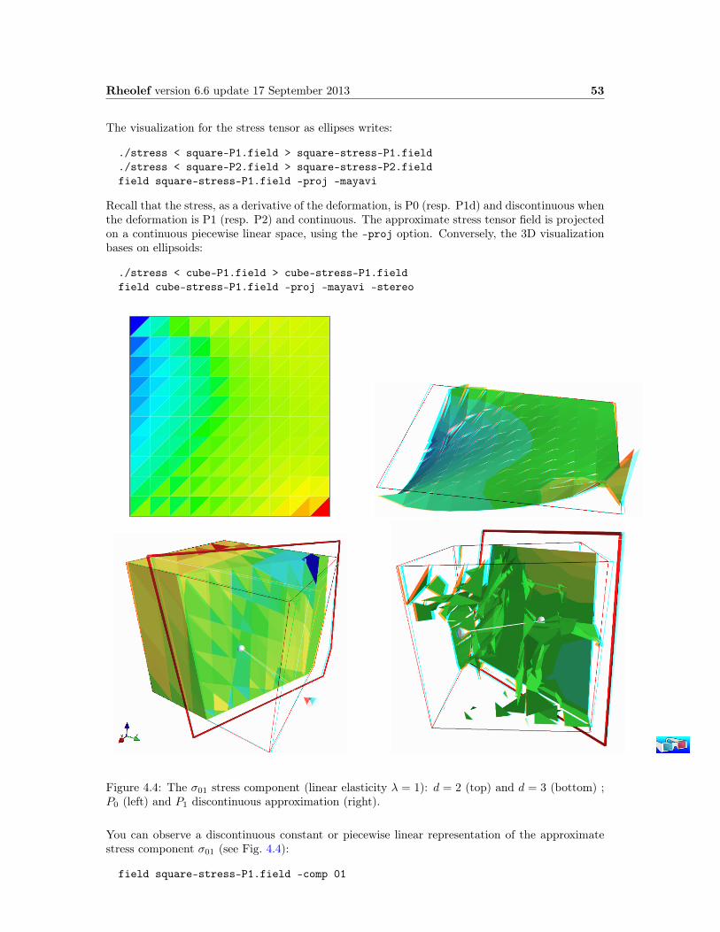
The visualization for the stress tensor as ellipses writes:
./stress < square-P1.field > square-stress-P1.field
./stress < square-P2.field > square-stress-P2.fieldfield square-stress-P1.field -proj -mayavi
Recall that the stress, as a derivative of the deformation, is P0 (resp. P1d) and discontinuous whenthe deformation is P1 (resp. P2) and continuous. The approximate stress tensor field is projectedon a continuous piecewise linear space, using the -proj option. Conversely, the 3D visualizationbases on ellipsoids:
./stress < cube-P1.field > cube-stress-P1.fieldfield cube-stress-P1.field -proj -mayavi -stereo
Figure 4.4: The σ01 stress component (linear elasticity λ = 1): d = 2 (top) and d = 3 (bottom) ;P0 (left) and P1 discontinuous approximation (right).
You can observe a discontinuous constant or piecewise linear representation of the approximatestress component σ01 (see Fig. 4.4):
field square-stress-P1.field -comp 01
54 Rheolef version 6.6 update 17 September 2013
field square-stress-P2.field -comp 01 -elevationfield square-stress-P2.field -comp 01 -elevation -stereo
Notice that the -stereo implies the -mayavi one, as this feature is not available with othersvisualization systems. The approximate stress field can be also projected on a continuous piecewisespace:
field square-stress-P2.field -comp 01 -elevation -proj
The tridimensional case writes simply (see Fig. 4.4):
./stress < cube-P1.field > cube-stress-P1.field
./stress < cube-P2.field > cube-stress-P2.fieldfield cube-stress-P1.field -comp 01 -stereofield cube-stress-P2.field -comp 01 -stereo -iso
and also the P1-projected versions write:
field cube-stress-P1.field -comp 01 -stereo -proj -isofield cube-stress-P2.field -comp 01 -stereo -proj -iso
These operations can be repeated for each σij components and for both P1 and P2 approximationof the deformation field.
4.3 Mesh adaptation
The main principle of the auto-adaptive mesh writes [6, 10,21,39,50]:
cin >> omega;uh = solve(omega);for (unsigned int i = 0; i < n; i++)
ch = criterion(uh);omega = adapt(ch);uh = solve(omega);
The initial mesh is used to compute a first solution. The adaptive loop compute an adaptivecriterion, denoted by ch, that depends upon the problem under consideration and the polynomialapproximation used. Then, a new mesh is generated, based on this criterion. A second solutionon an adapted mesh can be constructed. The adaptation loop converges generally in roughly 5 to20 iterations.Let us apply this principle to the elasticity problem.
Rheolef version 6.6 update 17 September 2013 55
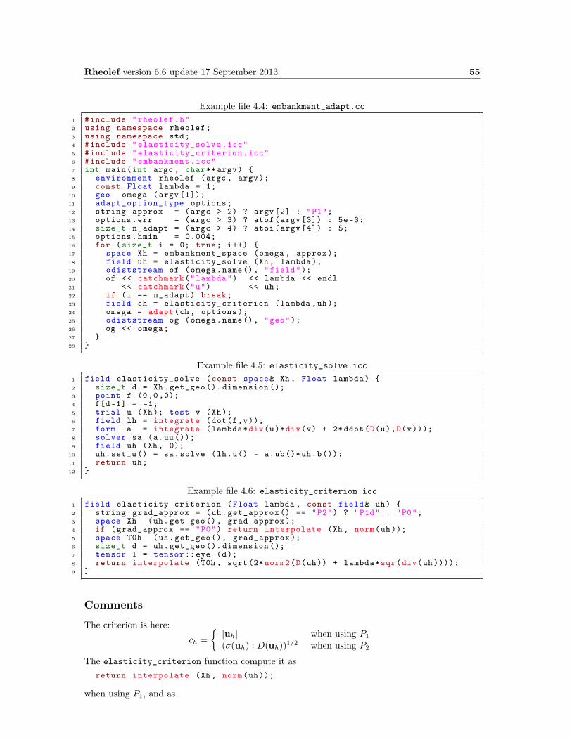
Example file 4.4: embankment_adapt.cc1 #include "rheolef.h"2 using namespace rheolef;3 using namespace std;4 #include "elasticity_solve.icc"5 #include "elasticity_criterion.icc"6 #include "embankment.icc"7 int main(int argc , char**argv) 8 environment rheolef (argc , argv);9 const Float lambda = 1;
10 geo omega (argv [1]);11 adapt_option_type options;12 string approx = (argc > 2) ? argv [2] : "P1";13 options.err = (argc > 3) ? atof(argv [3]) : 5e-3;14 size_t n_adapt = (argc > 4) ? atoi(argv [4]) : 5;15 options.hmin = 0.004;16 for (size_t i = 0; true; i++) 17 space Xh = embankment_space (omega , approx );18 field uh = elasticity_solve (Xh, lambda );19 odiststream of (omega.name(), "field");20 of << catchmark("lambda") << lambda << endl21 << catchmark("u") << uh;22 if (i == n_adapt) break;23 field ch = elasticity_criterion (lambda ,uh);24 omega = adapt(ch, options );25 odiststream og (omega.name(), "geo");26 og << omega;27 28
Example file 4.5: elasticity_solve.icc1 field elasticity_solve (const space& Xh , Float lambda) 2 size_t d = Xh.get_geo (). dimension ();3 point f (0,0,0);4 f[d-1] = -1;5 trial u (Xh); test v (Xh);6 field lh = integrate (dot(f,v));7 form a = integrate (lambda*div(u)*div(v) + 2*ddot(D(u),D(v)));8 solver sa (a.uu());9 field uh (Xh, 0);
10 uh.set_u () = sa.solve (lh.u() - a.ub()*uh.b());11 return uh;12
Example file 4.6: elasticity_criterion.icc1 field elasticity_criterion (Float lambda , const field& uh) 2 string grad_approx = (uh.get_approx () == "P2") ? "P1d" : "P0";3 space Xh (uh.get_geo(), grad_approx );4 if (grad_approx == "P0") return interpolate (Xh , norm(uh));5 space T0h (uh.get_geo(), grad_approx );6 size_t d = uh.get_geo (). dimension ();7 tensor I = tensor ::eye (d);8 return interpolate (T0h , sqrt (2* norm2(D(uh)) + lambda*sqr(div(uh ))));9
Comments
The criterion is here:
ch =
|uh| when using P1
(σ(uh) : D(uh))1/2 when using P2
The elasticity_criterion function compute it asreturn interpolate (Xh, norm(uh));
when using P1, and as
56 Rheolef version 6.6 update 17 September 2013
return interpolate (T0h , sqrt (2* norm2(D(uh)) + lambda*sqr(div(uh ))));
when using P2. The sqr function returns the square of a scalar. Conversely, the norm2 functionreturns the square of the norm. In the min programm, the result of the elasticity_criterionfunction is send to the adapt function:
field ch = elasticity_criterion (lambda , uh);omega = adapt (ch , options );
The adapt_option_type declaration is used by Rheolef to send options to the mesh generator.The err parameter controls the error via the edge length of the mesh: the smaller it is, the smallerthe edges of the mesh are. In our example, is set by default to one. Conversely, the hmin parametercontrols minimal edge length.
How to run the program
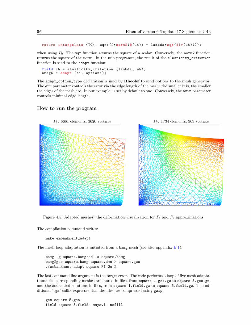
P1: 6661 elements, 3620 vertices P2: 1734 elements, 969 vertices
Figure 4.5: Adapted meshes: the deformation visualization for P1 and P2 approximations.
The compilation command writes:
make embankment_adapt
The mesh loop adaptation is initiated from a bamg mesh (see also appendix B.1).
bamg -g square.bamgcad -o square.bamgbamg2geo square.bamg square.dmn > square.geo./embankment_adapt square P1 2e-2
The last command line argument is the target error. The code performs a loop of five mesh adapta-tions: the corresponding meshes are stored in files, from square-1.geo.gz to square-5.geo.gz,and the associated solutions in files, from square-1.field.gz to square-5.field.gz. The ad-ditional ‘.gz’ suffix expresses that the files are compressed using gzip.
geo square-5.geofield square-5.field -mayavi -nofill
Rheolef version 6.6 update 17 September 2013 57
Note that the ‘.gz’ suffix is automatically assumed by the geo and the field commands.For a piecewise quadratic approximation:
./embankment_adapt square P2 5e-3
Then, the visualization writes:
geo square-5.geofield square-5.field -mayavi -nofill
A one-dimensional mesh adaptive procedure is also possible:
gmsh -1 line.mshcad -o line.mshmsh2geo line.msh > line.geogeo line.geo./embankment_adapt line P2geo line-5.geofield line-5.field -comp 0 -elevation
The three-dimensional extension of this mesh adaptive procedure is in development.
4.4 The Stokes problem
Formulation
Let us consider the Stokes problem for the driven cavity in Ω =]0, 1[d, d = 2, 3. The problemwrites:
(S) find u = (u0, . . . , ud−1) and p defined in Ω such that:
− div(2D(u)) + ∇p = 0 in Ω,− divu = 0 in Ω,
u = (1, 0) on Γtop,u = 0 on Γleft ∪ Γright ∪ Γbottom,∂u0
∂n=
∂u1
∂n= u2 = 0 on Γback ∪ Γfront when d = 3,
where D(u) = (∇u + ∇uT )/2. The boundaries are represented on Fig. 4.1, page 48.The variational formulation of this problem expresses:
(V FS) find u ∈ V(1) and p ∈ L20(Ω) such that:
a(u,v) + b(v, p) = 0, ∀v ∈ V(0),b(u, q) = 0, ∀q ∈ L2
0(Ω),
where
a(u,v) =
∫
Ω
2D(u) : D(v) dx,
b(v, q) = −∫
Ω
div(v) q dx.
V(α) = v ∈ (H1(Ω))2; v = 0 on Γleft ∪ Γright ∪ Γbottom and v = (α, 0) on Γtop, when d = 2,
V(α) = v ∈ (H1(Ω))3; v = 0 on Γleft ∪ Γright ∪ Γbottom,
v = (α, 0, 0) on Γtop and v2 = 0 on Γback ∪ Γfront, when d = 3,
L20(Ω) = q ∈ L2(Ω);
∫
Ω
q dx = 0.
58 Rheolef version 6.6 update 17 September 2013
Approximation
The Taylor-Hood [22] finite element approximation of the Stokes problem is considered. Weintroduce a mesh Th of Ω and the following finite dimensional spaces:
Xh = v ∈ (H1(Ω))d; v/K ∈ (P2)d, ∀K ∈ Th,Vh(α) = Xh ∩V(α),
Qh = q ∈ L2(Ω)) ∩ C0(Ω); q/K ∈ P1, ∀K ∈ Th,
The approximate problem writes:(V FS)h find uh ∈ Vh(1) and p ∈ Qh such that:
a(uh,v) + b(v, ph) = 0, ∀v ∈ Vh(0),b(uh, q) = 0, ∀q ∈ Qh. (4.4)
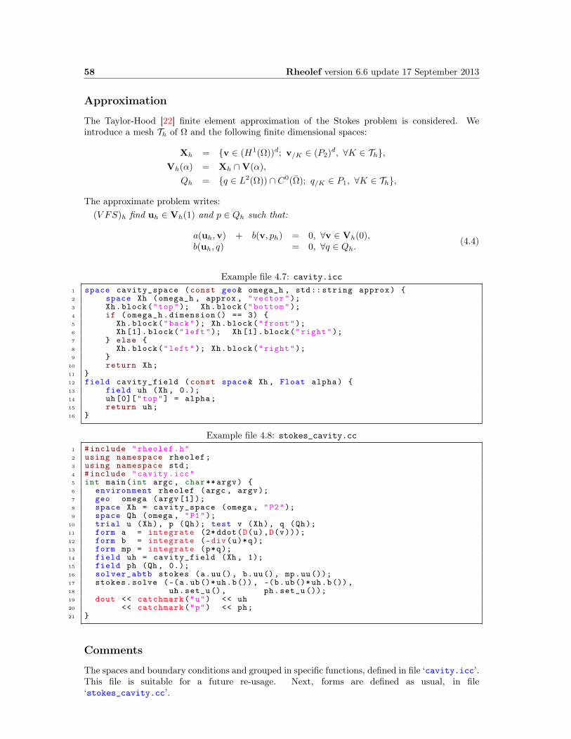
Example file 4.7: cavity.icc1 space cavity_space (const geo& omega_h , std:: string approx) 2 space Xh (omega_h , approx , "vector");3 Xh.block("top"); Xh.block("bottom");4 if (omega_h.dimension () == 3) 5 Xh.block("back"); Xh.block("front");6 Xh[1]. block("left"); Xh[1]. block("right");7 else 8 Xh.block("left"); Xh.block("right");9
10 return Xh;11 12 field cavity_field (const space& Xh, Float alpha) 13 field uh (Xh, 0.);14 uh[0]["top"] = alpha;15 return uh;16
Example file 4.8: stokes_cavity.cc1 #include "rheolef.h"2 using namespace rheolef;3 using namespace std;4 #include "cavity.icc"5 int main(int argc , char**argv) 6 environment rheolef (argc , argv);7 geo omega (argv [1]);8 space Xh = cavity_space (omega , "P2");9 space Qh (omega , "P1");
10 trial u (Xh), p (Qh); test v (Xh), q (Qh);11 form a = integrate (2* ddot(D(u),D(v)));12 form b = integrate (-div(u)*q);13 form mp = integrate (p*q);14 field uh = cavity_field (Xh, 1);15 field ph (Qh, 0.);16 solver_abtb stokes (a.uu(), b.uu(), mp.uu());17 stokes.solve (-(a.ub()*uh.b()), -(b.ub()*uh.b()),18 uh.set_u(), ph.set_u ());19 dout << catchmark("u") << uh20 << catchmark("p") << ph;21
Comments
The spaces and boundary conditions and grouped in specific functions, defined in file ‘cavity.icc’.This file is suitable for a future re-usage. Next, forms are defined as usual, in file‘stokes_cavity.cc’.
Rheolef version 6.6 update 17 September 2013 59
The problem admits the following matrix form:(
a.uu trans(b.uu)b.uu 0
)(uh.uph.u
)=
(−a.ub ∗ uh.b−b.ub ∗ uh.b
)
An initial value for the pressure field is provided:field ph (Qh, 0);
The main Stokes solver call writes:solver_abtb stokes (a.uu(), b.uu(), mp.uu());stokes.solve (-(a.ub()*uh.b()), -(b.ub()*uh.b()),
uh.set_u(), ph.set_u ());
For tridimensional geometries (d = 3), this system is solved by the preconditioned conjugategradient algorithm. the preconditioner is here the mass matrix mp.uu for the pressure: as showedin [24], the number of iterations need by the conjugate gradient algorithm to reach a given precisionis then independent of the mesh size. For more details, see the Rheolef reference manual relatedto mixed solvers, available e.g. via the unix command:
man solver_abtb
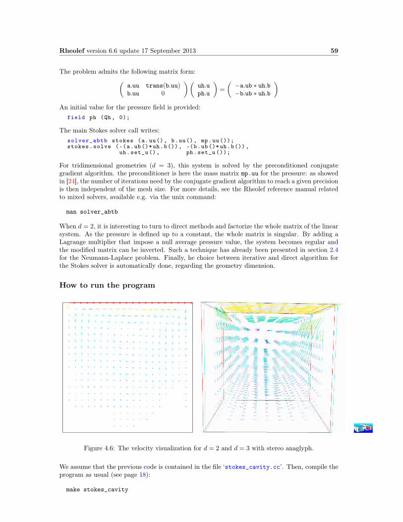
When d = 2, it is interesting to turn to direct methods and factorize the whole matrix of the linearsystem. As the pressure is defined up to a constant, the whole matrix is singular. By adding aLagrange multiplier that impose a null average pressure value, the system becomes regular andthe modified matrix can be inverted. Such a technique has already been presented in section 2.4for the Neumann-Laplace problem. Finally, he choice between iterative and direct algorithm forthe Stokes solver is automatically done, regarding the geometry dimension.
How to run the program
Figure 4.6: The velocity visualization for d = 2 and d = 3 with stereo anaglyph.
We assume that the previous code is contained in the file ‘stokes_cavity.cc’. Then, compile theprogram as usual (see page 18):
make stokes_cavity

60 Rheolef version 6.6 update 17 September 2013
and enter the commands:
mkgeo_grid -t 10 > square.geo./stokes_cavity square > square.field
The previous command solves the problem for the corresponding mesh and writes the solution ina ‘.field’ file. Run the velocity vector visualization :
field square.field -velocity
Run also some scalar visualizations:
field square.field -comp 0field square.field -comp 1field square.field -catchmark p
Note the -catchmark option to the field command: the file reader jumps to the label and thenstarts to read the selected field. Next, perform another computation on a finer mesh:
mkgeo_grid -t 20 > square-20.geo./stokes_cavity square-20.geo > square-20.field
and observe the convergence.Finally, let us consider the three dimensional case:
mkgeo_grid -T 5 > cube.geo./stokes_cavity cube.geo > cube.field
and the corresponding visualization:
field cube.field -velocityfield cube.field -comp 0field cube.field -comp 1field cube.field -comp 2field cube.field -catchmark p
4.5 Computing the vorticity
Formulation and approximation
When d = 2, we define [19, page 30] for any distributions φ and v:
curlφ =
(∂φ
∂x1, − ∂φ
∂x0
),
curlv =∂v1
∂x0− ∂v0
∂x1,
and when d = 3:
curl v =
(∂v2
∂x1− ∂v1
∂x2,∂v0
∂x2− ∂v2
∂x0,∂v1
∂x0− ∂v0
∂x1
)
Let u be the solution of the Stokes problem (S). The vorticity is defined by:
ω = curlu when d = 2,ω = curl u when d = 3.

Rheolef version 6.6 update 17 September 2013 61
Since the approximation of the velocity is piecewise quadratic, we are looking for a discontinuouspiecewise linear vorticity field that belongs to:
Yh = ξ ∈ L2(Ω); ξ/K ∈ P1, ∀K ∈ Th, when d = 2Yh = ξ ∈ (L2(Ω))3; ξi/K ∈ P1, ∀K ∈ Th, when d = 3
The approximate variational formulation writes:
ωh ∈ Yh,∫
Ωωh ξ dx =
∫Ω
curluh ξ dx, ∀ξ ∈ Yh when d = 2,
ω ∈ Yh,∫
Ωωh.ξ dx =
∫Ωcurl uh.ξ dx, ∀ξ ∈ Yh when d = 3.
Example file 4.9: vorticity.cc1 #include "rheolef.h"2 using namespace rheolef;3 using namespace std;4 int main(int argc , char** argv) 5 environment rheolef (argc , argv);6 field uh;7 din >> uh;8 const space& Xh = uh.get_space ();9 string grad_approx = "P" + itos(Xh.degree ()-1) + "d";
10 string valued = (uh.size() == 3) ? "vector" : "scalar";11 space Lh (uh.get_geo(), grad_approx , valued );12 field curl_uh = interpolate (Lh, curl(uh));13 dout << catchmark("w") << curl_uh;14
Comments
As for the stress tensor (see stress.cc, page 52), the vorticity is obtained by a direct interpolationof the uh first derivatives and its approximation is discontinuous at inter-element boundaries.
How to run the program
Figure 4.7: The vorticity: elevation view for d = 2 and vector representation for d = 3 (withanaglyph).
62 Rheolef version 6.6 update 17 September 2013
For d = 2, just enter:
make vorticity./vorticity < square.field | field -elevation -stereo -
and you observe a discontinuous piecewise linear representation of the approximate vorticity. Also,the vorticity presents two sharp peaks at the upper corners of the driven cavity: the vorticity isunbounded and the peaks will increase with mesh refinements. This singularity of the solution isdue to the boundary condition for the first component of the velocity u0 that jumps from zero toone at the corners. The approximate vorticity field can also be projected on a continuous piecewiselinear space, using the -proj option (See Fig. 4.7 left):
./vorticity < square.field | field -elevation -stereo -nofill -
./vorticity < square.field | field -elevation -stereo -proj -
For d = 3, the whole vorticity vector can also be visualized (See Fig. 4.7 right):
./vorticity < cube.field | field -proj -velocity -stereo -
In the previous command, the -proj option has been used: since the 3D render has no support fordiscontinuous piecewise linear fields, the P1-discontinuous field is transformed into a P1-continuousone, thanks to a L2 projection. P1 The following command shows the second component of thevorticity vector, roughly similar to the bidimensional case.
./vorticity < cube.field | field -comp 1 -
./vorticity < cube.field | field -comp 1 -proj -
4.6 Computing the stream function
Formulation and approximation
When d = 3, the stream function is a vector-valued field ψ that satisfies [19, page 90]: curlψ = uand divψ = 0. From the identity:
curl curlψ = −∆ψ +∇(divψ)
we obtain the following characterization of ψ :
−∆ψ = curl u in Ω,ψ = 0 on Γback ∪ Γfront ∪ Γtop ∪ Γbottom,
∂ψ
∂n= 0 on Γleft ∪ Γright.
When d = 2, the stream function ψ is a scalar-valued field the solution of the following problem [19,page 88]:
−∆ψ = curlu in Ω,ψ = 0 on ∂Ω.

Rheolef version 6.6 update 17 September 2013 63
Example file 4.10: streamf_cavity.cc1 #include "rheolef.h"2 using namespace rheolef;3 using namespace std;4 int main (int argc , char** argv) 5 environment rheolef (argc , argv);6 field uh;7 din >> uh;8 const space& Xh = uh.get_space ();9 size_t d = uh.get_geo (). dimension ();
10 string valued = (d == 3) ? "vector" : "scalar";11 space Ph (uh.get_geo(), "P2", valued );12 Ph.block("top"); Ph.block("bottom");13 if (d == 3) 14 Ph.block("back"); Ph.block("front");15 else 16 Ph.block("left"); Ph.block("right");17 18 trial u (Xh), psi (Ph); test phi (Ph);19 form a = (d == 3) ? integrate (ddot(grad(psi),grad(phi)))20 : integrate ( dot(grad(psi),grad(phi )));21 form b = (d==3) ? integrate (dot(curl(u),phi))22 : integrate (curl(u)*phi);23 field psi_h (Ph, 0.);24 field lh = b*uh;25 solver sa (a.uu());26 psi_h.set_u() = sa.solve (lh.u() - a.ub()* psi_h.b());27 dout << catchmark("psi") << psi_h;28
How to run the program
Figure 4.8: The stream function visualization: isolines for d = 2, and combined vectors andisonorm surface for d = 3.
For d = 2, just enter (see Fig. 4.8 left):
make streamf_cavity./streamf_cavity < square.field | field -bw -
64 Rheolef version 6.6 update 17 September 2013
For d = 3, the whole stream function vector can be visualized:
./streamf_cavity < cube.field | field -velocity -
The second component of the stream function is showed by:
./streamf_cavity < cube.field | field -comp 1 -
The combined representation of Fig. 4.8.right has been obtained in two steps. First, enter:
./streamf_cavity < cube.field | field -comp 1 -noclean -noexecute -mv output.vtk psi1.vtk./streamf_cavity < cube.field | field -velocity -
The -noclean -noexecute options cause the creation of the ‘.vtk’ file for the second compo-nent, without running the mayavi visualization. Next, in the mayavi window associated to thewhole stream function, select the File/Load data/VTK file menu and load ‘psi1.vtk’. Finally,select the Vizualize/Module/IsoSurface menu. Observe that the 3D stream function is mainlyrepresented by its second component.

Chapter 5
Nearly incompressible elasticity andthe stabilized Stokes problems
5.1 The incompressible elasticity problem
Formulation
Let us go back to the linear elasticity problem.When λ becomes large, this problem is related to the incompressible elasticity and cannot besolved as it was previously done. To overcome this difficulty, the pressure is introduced :
p = −λdivu
and the problem becomes:(E) find u and p defined in Ω such that:
− div(2D(u)) + ∇p = f in Ω,
− divu − 1
λp = 0 in Ω,
+B.C.
The variational formulation of this problem expresses:(V FE) find u ∈ V (1) and p ∈ L2(Ω) such that:
a(u,v) + b(v, p) = m(f ,v), ∀v ∈ V (0),b(u, q) − c(p, q) = 0, ∀q ∈ L2
0(Ω),
where
m(u,v) =
∫
Ω
u.v dx,
a(u,v) =
∫
Ω
D(u) : D(v) dx,
b(v, q) = −∫
Ω
div(v) q dx.
c(p, q) =1
λ
∫
Ω
p q dx.
V = v ∈ (H1(Ω))2; v = 0 on Γleft ∪ ΓbottomWhen λ becomes large, we obtain the incompressible elasticity problem, that coincides with theStokes problem.
65
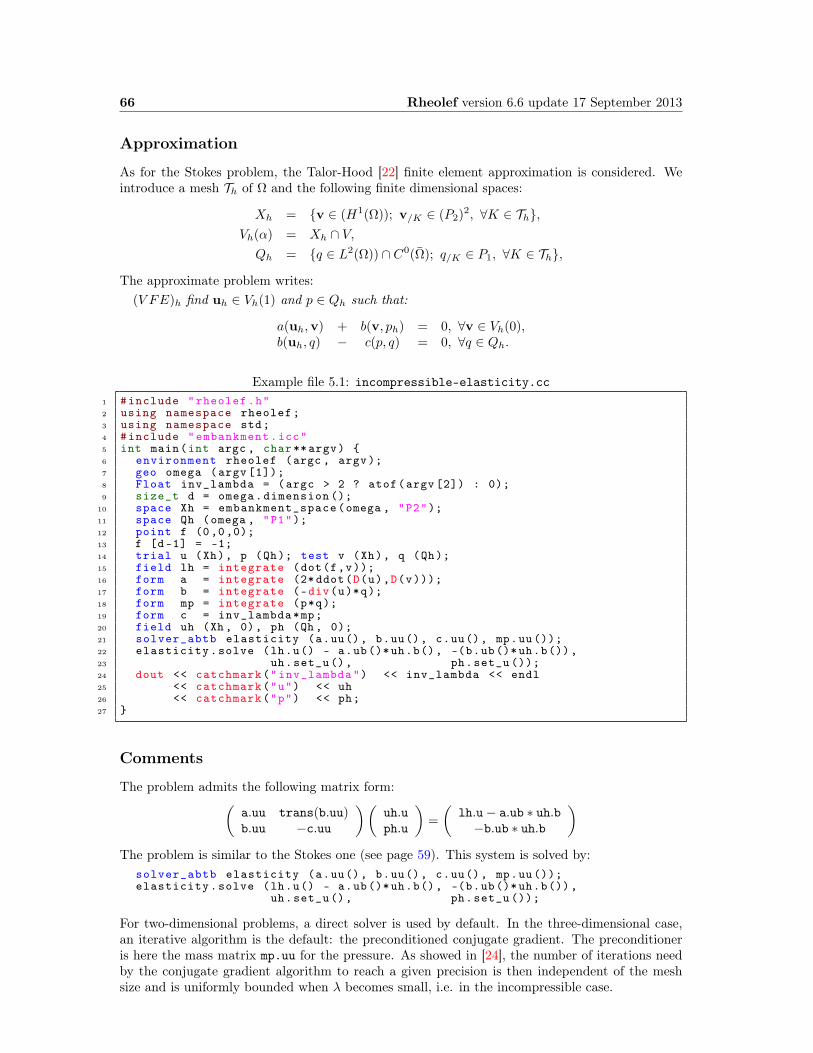
66 Rheolef version 6.6 update 17 September 2013
Approximation
As for the Stokes problem, the Talor-Hood [22] finite element approximation is considered. Weintroduce a mesh Th of Ω and the following finite dimensional spaces:
Xh = v ∈ (H1(Ω)); v/K ∈ (P2)2, ∀K ∈ Th,Vh(α) = Xh ∩ V,Qh = q ∈ L2(Ω)) ∩ C0(Ω); q/K ∈ P1, ∀K ∈ Th,
The approximate problem writes:(V FE)h find uh ∈ Vh(1) and p ∈ Qh such that:
a(uh,v) + b(v, ph) = 0, ∀v ∈ Vh(0),b(uh, q) − c(p, q) = 0, ∀q ∈ Qh.
Example file 5.1: incompressible-elasticity.cc1 #include "rheolef.h"2 using namespace rheolef;3 using namespace std;4 #include "embankment.icc"5 int main(int argc , char**argv) 6 environment rheolef (argc , argv);7 geo omega (argv [1]);8 Float inv_lambda = (argc > 2 ? atof(argv [2]) : 0);9 size_t d = omega.dimension ();
10 space Xh = embankment_space(omega , "P2");11 space Qh (omega , "P1");12 point f (0,0,0);13 f [d-1] = -1;14 trial u (Xh), p (Qh); test v (Xh), q (Qh);15 field lh = integrate (dot(f,v));16 form a = integrate (2* ddot(D(u),D(v)));17 form b = integrate (-div(u)*q);18 form mp = integrate (p*q);19 form c = inv_lambda*mp;20 field uh (Xh, 0), ph (Qh, 0);21 solver_abtb elasticity (a.uu(), b.uu(), c.uu(), mp.uu());22 elasticity.solve (lh.u() - a.ub()*uh.b(), -(b.ub()*uh.b()),23 uh.set_u(), ph.set_u ());24 dout << catchmark("inv_lambda") << inv_lambda << endl25 << catchmark("u") << uh26 << catchmark("p") << ph;27
Comments
The problem admits the following matrix form:(
a.uu trans(b.uu)b.uu −c.uu
)(uh.uph.u
)=
(lh.u− a.ub ∗ uh.b−b.ub ∗ uh.b
)
The problem is similar to the Stokes one (see page 59). This system is solved by:solver_abtb elasticity (a.uu(), b.uu(), c.uu(), mp.uu());elasticity.solve (lh.u() - a.ub()*uh.b(), -(b.ub()*uh.b()),
uh.set_u(), ph.set_u ());
For two-dimensional problems, a direct solver is used by default. In the three-dimensional case,an iterative algorithm is the default: the preconditioned conjugate gradient. The preconditioneris here the mass matrix mp.uu for the pressure. As showed in [24], the number of iterations needby the conjugate gradient algorithm to reach a given precision is then independent of the meshsize and is uniformly bounded when λ becomes small, i.e. in the incompressible case.
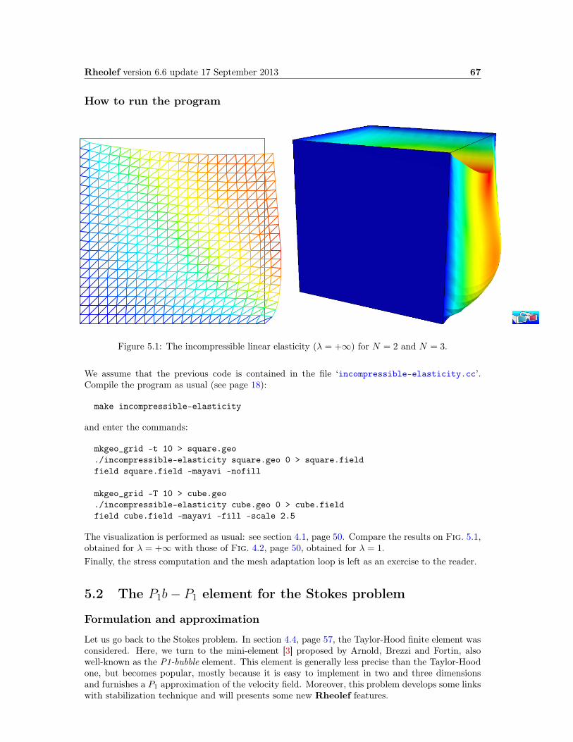
Rheolef version 6.6 update 17 September 2013 67
How to run the program
Figure 5.1: The incompressible linear elasticity (λ = +∞) for N = 2 and N = 3.
We assume that the previous code is contained in the file ‘incompressible-elasticity.cc’.Compile the program as usual (see page 18):
make incompressible-elasticity
and enter the commands:
mkgeo_grid -t 10 > square.geo./incompressible-elasticity square.geo 0 > square.fieldfield square.field -mayavi -nofill
mkgeo_grid -T 10 > cube.geo./incompressible-elasticity cube.geo 0 > cube.fieldfield cube.field -mayavi -fill -scale 2.5
The visualization is performed as usual: see section 4.1, page 50. Compare the results on Fig. 5.1,obtained for λ = +∞ with those of Fig. 4.2, page 50, obtained for λ = 1.Finally, the stress computation and the mesh adaptation loop is left as an exercise to the reader.
5.2 The P1b− P1 element for the Stokes problem
Formulation and approximation
Let us go back to the Stokes problem. In section 4.4, page 57, the Taylor-Hood finite element wasconsidered. Here, we turn to the mini-element [3] proposed by Arnold, Brezzi and Fortin, alsowell-known as the P1-bubble element. This element is generally less precise than the Taylor-Hoodone, but becomes popular, mostly because it is easy to implement in two and three dimensionsand furnishes a P1 approximation of the velocity field. Moreover, this problem develops some linkswith stabilization technique and will presents some new Rheolef features.
68 Rheolef version 6.6 update 17 September 2013
We consider a mesh Th of Ω ⊂ Rd, d = 2, 3 composed only of simplicial elements: triangles whend = 2 and tetrahedra when d = 3. The following finite dimensional spaces are introduced:
X(1)h = v ∈ (H1(Ω))d; v/K ∈ (P1)d, ∀K ∈ Th,Bh = β ∈ (C0(Ω))d; β/K ∈ B(K)d,∀K ∈ ThXh = X
(1)h ⊕Bh
Vh(α) = Xh ∩V(α),
Qh = q ∈ L2(Ω)) ∩ C0(Ω); q/K ∈ P1, ∀K ∈ Th,
where B(K) = vect(λ1 × . . . × λd+1) and λi are the barycentric coordinates of the simplex K.The B(K) space is related to the bubble local space. The approximate problem is similar to (4.4),page 58, up to the choice of finite dimensional spaces.
Remark that the velocity field splits in two terms: uh = u(1)h +u
(b)h , where u(1)
h ∈ X(1)h is continuous
and piecewise linear, and u(b)h ∈ Bh is the bubble term.
We consider the abrupt contraction geometry:
Ω =]−Lu, 0[×]0, c[ ∪ [0, Ld[×]0, 1[
where c > 1 stands for the contraction ratio, and Lu, Ld > 0, are the upstream and downstreamtube lengths. The boundary conditions on u = (u0, u1) for this test case are:
u0 = upoiseuille and u1 = 0 on Γupstream
u = 0 on Γwall
∂u0
∂x1= 0 and u1 = 0 on Γaxis
∂u
∂n= 0 on Γdownstream
where
Γupstream = −Lu×]0, c[
Γdownstream = Ld×]0, 1[
Γaxis = ]−Lu, Ld[×0Γwall = ]−Lu, 0[×c ∪ 0×]1, c[ ∪ ]0, Ld[×1
The matrix structure is similar to those of the Taylor-Hood element (see section 4.4, page 57).Since Xh = X
(1)h ⊕ Bh, any element uh ∈ Xh can be written as a sum uh = u1,h + ub,h where
u1,h ∈ X(1)h and ub,h ∈ Bh. Remark that
a(u1,h, vb,h) = 0, ∀u1,h ∈ X(1)h , ∀vb,h ∈ Bh.
Thus, the form a(., .) defined over Xh × Xh writes simply as the sum of the forms a1(., .) andab(., .), defined over X
(1)h ×X
(1)h and Bh × Bh respectively. Finaly, the form b(., .) defined over
Xh ×Qh writes as the sum of the forms b1(., .) and bb(., .), defined over X(1)h ×Qh and Bh ×Qh
respectively. Then, the linear system admits the following block structure :
A1 0 BT10 Ab BTbB1 Bb 0
U1
UbP
=
L1
LbLp
An alternative and popular implementation of this element eliminates the unknowns related tothe bubble components (see e.g. [1], page 24). Remark that, on any element K ∈ Th, any bubble

Rheolef version 6.6 update 17 September 2013 69
function vK that belongs to B(K) vanishes on the boundary of K and have a compact support inK. Thus, the Ab matrix is block-diagonal. Moreover, Ab is invertible and Ub writes :
Ub = A−1b (BTb p− Lb)
As Ab is block-diagonal, its inverse can be efficiently inverted at the element level during theassembly process. Then, Ub can be easily eliminated from the system that reduces to:
(A1 BT1B1 −C
)(U1
P
)=
(L1
Lp
)
where Lp = Lp − A−1b Lp and C = BbA
−1b BTb . Remarks that the matrix structure is similar to
those of the nearly incompressible elasticity (see 5.1, page 5.1). This reduced matrix formulationof the P1b − P1 element is similar to the direct P1 − P1 stabilized element, proposed by Brezziand Pitkäranta [9].
Example file 5.2: stokes_contraction_bubble.cc1 #include "rheolef.h"2 using namespace rheolef;3 using namespace std;4 #include "poiseuille.h"5
6 int main(int argc , char**argv) 7 environment rheolef (argc , argv);8 geo omega (argv [1]);9 space X1h (omega , "P1", "vector");
10 space Bh (omega , "bubble", "vector");11 space Qh (omega , "P1");12 space Wh (omega["upstream"], "P1");13 X1h.block ("wall");14 X1h.block ("upstream");15 X1h [1]. block ("axis");16 X1h [1]. block ("downstream");17 trial u1 (X1h), ub (Bh), p (Qh);18 test v1 (X1h), vb (Bh), q (Qh);19 form mp = integrate (p*q);20 form b1 = integrate (-div(u1)*q);21 form bb = integrate (-div(ub)*q);22 form a1 = integrate (2* ddot(D(u1),D(v1)));23 form_option_type fopt;24 fopt.invert = true;25 form inv_ab = integrate (2* ddot(D(ub),D(vb)), fopt);26 form c = bb*inv_ab*trans(bb);27 field u1h (X1h , 0), ph (Qh, 0);28 string sys_coord = omega.coordinate_system_name ();29 Float cr = omega.xmax ()[1];30 u1h [0]["upstream"] = interpolate (Wh , u_poiseuille(cr ,sys_coord ));31 solver_abtb stokes (a1.uu(), b1.uu(), c.uu(), mp.uu());32 stokes.solve (-(a1.ub()*u1h.b()), -(b1.ub()*u1h.b()),33 u1h.set_u(), ph.set_u ());34 dout << catchmark("inv_lambda") << 0 << endl35 << catchmark("u") << u1h36 << catchmark("p") << ph;37
Comments
First, A−1b is computed as:
form_option_type fopt;fopt.invert = true;form inv_ab = integrate (2* ddot(D(ub),D(vb)), fopt);
Notice the usage of the optional parameter fopt to the integrate function. As the form isbloc-diagonal, its inverse is computed element-by-element during the assembly process. Next, theC = BbA
−1b BTb form is simply computed as:
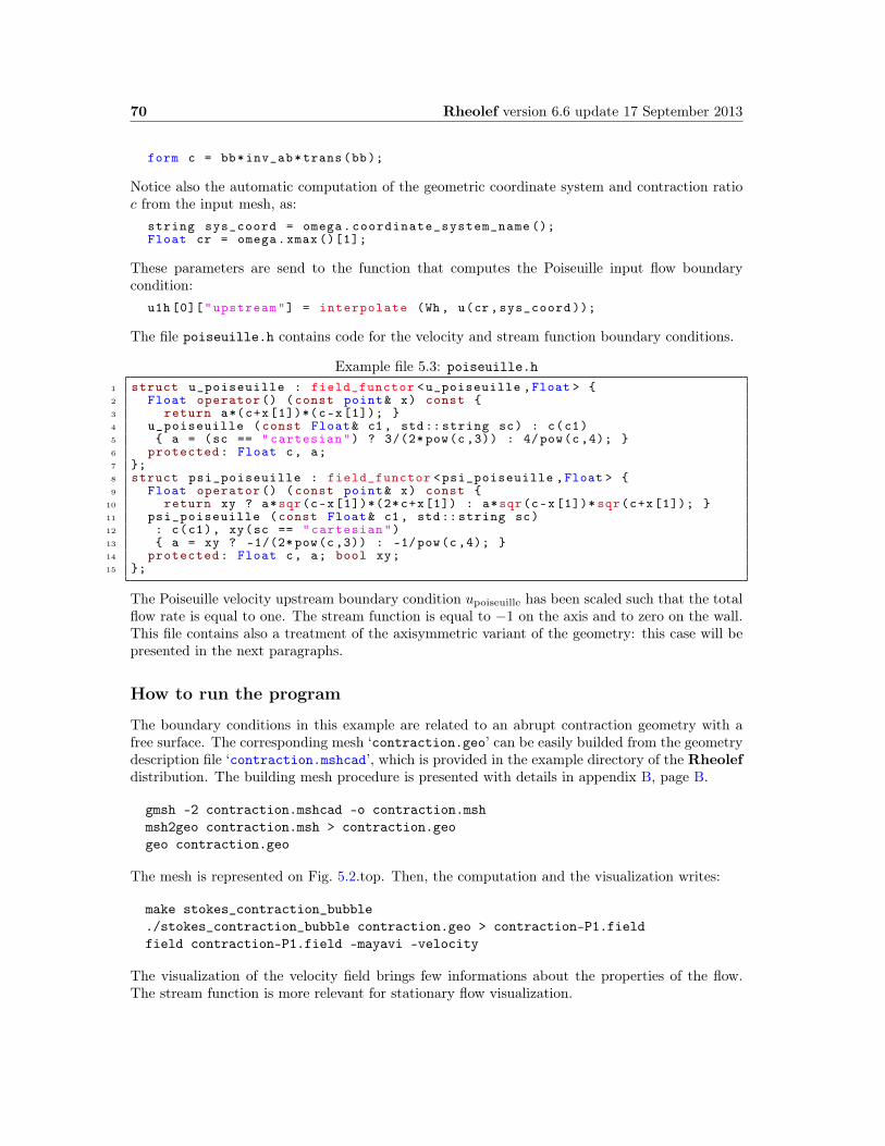
70 Rheolef version 6.6 update 17 September 2013
form c = bb*inv_ab*trans(bb);
Notice also the automatic computation of the geometric coordinate system and contraction ratioc from the input mesh, as:
string sys_coord = omega.coordinate_system_name ();Float cr = omega.xmax ()[1];
These parameters are send to the function that computes the Poiseuille input flow boundarycondition:
u1h [0]["upstream"] = interpolate (Wh , u(cr,sys_coord ));
The file poiseuille.h contains code for the velocity and stream function boundary conditions.
Example file 5.3: poiseuille.h1 struct u_poiseuille : field_functor <u_poiseuille ,Float > 2 Float operator () (const point& x) const 3 return a*(c+x[1])*(c-x[1]); 4 u_poiseuille (const Float& c1 , std:: string sc) : c(c1)5 a = (sc == "cartesian") ? 3/(2* pow(c,3)) : 4/pow(c,4); 6 protected: Float c, a;7 ;8 struct psi_poiseuille : field_functor <psi_poiseuille ,Float > 9 Float operator () (const point& x) const
10 return xy ? a*sqr(c-x[1])*(2*c+x[1]) : a*sqr(c-x[1])* sqr(c+x[1]); 11 psi_poiseuille (const Float& c1 , std:: string sc)12 : c(c1), xy(sc == "cartesian")13 a = xy ? -1/(2* pow(c,3)) : -1/pow(c,4); 14 protected: Float c, a; bool xy;15 ;
The Poiseuille velocity upstream boundary condition upoiseuille has been scaled such that the totalflow rate is equal to one. The stream function is equal to −1 on the axis and to zero on the wall.This file contains also a treatment of the axisymmetric variant of the geometry: this case will bepresented in the next paragraphs.
How to run the program
The boundary conditions in this example are related to an abrupt contraction geometry with afree surface. The corresponding mesh ‘contraction.geo’ can be easily builded from the geometrydescription file ‘contraction.mshcad’, which is provided in the example directory of the Rheolefdistribution. The building mesh procedure is presented with details in appendix B, page B.
gmsh -2 contraction.mshcad -o contraction.mshmsh2geo contraction.msh > contraction.geogeo contraction.geo
The mesh is represented on Fig. 5.2.top. Then, the computation and the visualization writes:
make stokes_contraction_bubble./stokes_contraction_bubble contraction.geo > contraction-P1.fieldfield contraction-P1.field -mayavi -velocity
The visualization of the velocity field brings few informations about the properties of the flow.The stream function is more relevant for stationary flow visualization.
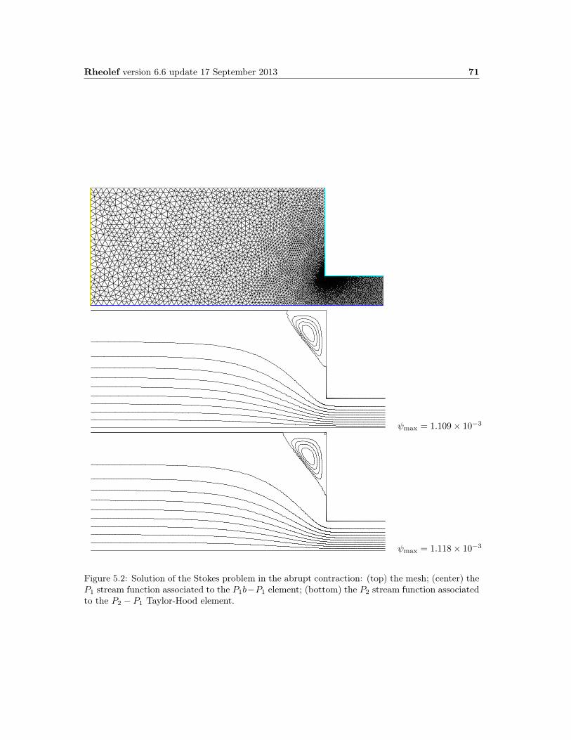
Rheolef version 6.6 update 17 September 2013 71
ψmax = 1.109× 10⁻³
ψmax = 1.118× 10⁻³
Figure 5.2: Solution of the Stokes problem in the abrupt contraction: (top) the mesh; (center) theP1 stream function associated to the P1b−P1 element; (bottom) the P2 stream function associatedto the P2 − P1 Taylor-Hood element.
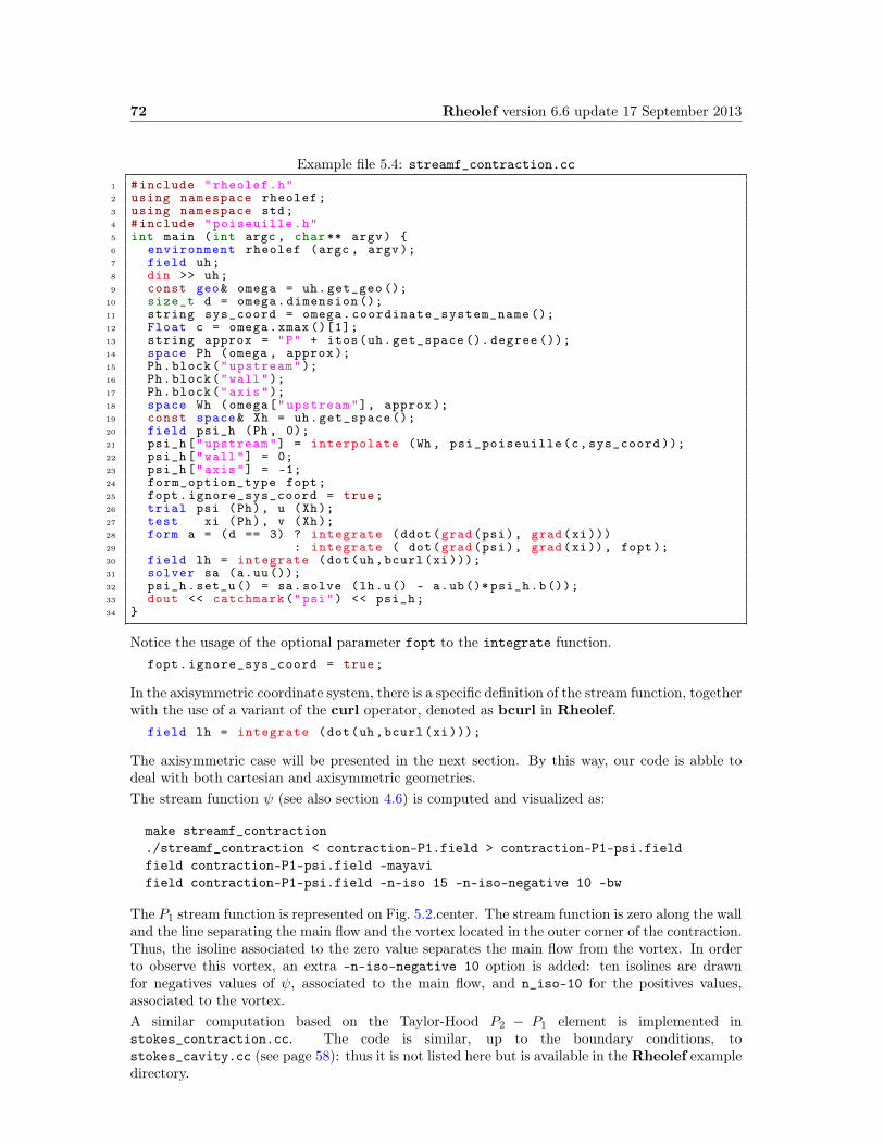
72 Rheolef version 6.6 update 17 September 2013
Example file 5.4: streamf_contraction.cc1 #include "rheolef.h"2 using namespace rheolef;3 using namespace std;4 #include "poiseuille.h"5 int main (int argc , char** argv) 6 environment rheolef (argc , argv);7 field uh;8 din >> uh;9 const geo& omega = uh.get_geo ();
10 size_t d = omega.dimension ();11 string sys_coord = omega.coordinate_system_name ();12 Float c = omega.xmax ()[1];13 string approx = "P" + itos(uh.get_space (). degree ());14 space Ph (omega , approx );15 Ph.block("upstream");16 Ph.block("wall");17 Ph.block("axis");18 space Wh (omega["upstream"], approx );19 const space& Xh = uh.get_space ();20 field psi_h (Ph, 0);21 psi_h["upstream"] = interpolate (Wh, psi_poiseuille(c,sys_coord ));22 psi_h["wall"] = 0;23 psi_h["axis"] = -1;24 form_option_type fopt;25 fopt.ignore_sys_coord = true;26 trial psi (Ph), u (Xh);27 test xi (Ph), v (Xh);28 form a = (d == 3) ? integrate (ddot(grad(psi), grad(xi)))29 : integrate ( dot(grad(psi), grad(xi)), fopt);30 field lh = integrate (dot(uh,bcurl(xi)));31 solver sa (a.uu());32 psi_h.set_u() = sa.solve (lh.u() - a.ub()* psi_h.b());33 dout << catchmark("psi") << psi_h;34
Notice the usage of the optional parameter fopt to the integrate function.fopt.ignore_sys_coord = true;
In the axisymmetric coordinate system, there is a specific definition of the stream function, togetherwith the use of a variant of the curl operator, denoted as bcurl in Rheolef.
field lh = integrate (dot(uh,bcurl(xi)));
The axisymmetric case will be presented in the next section. By this way, our code is abble todeal with both cartesian and axisymmetric geometries.The stream function ψ (see also section 4.6) is computed and visualized as:
make streamf_contraction./streamf_contraction < contraction-P1.field > contraction-P1-psi.fieldfield contraction-P1-psi.field -mayavifield contraction-P1-psi.field -n-iso 15 -n-iso-negative 10 -bw
The P1 stream function is represented on Fig. 5.2.center. The stream function is zero along the walland the line separating the main flow and the vortex located in the outer corner of the contraction.Thus, the isoline associated to the zero value separates the main flow from the vortex. In orderto observe this vortex, an extra -n-iso-negative 10 option is added: ten isolines are drawnfor negatives values of ψ, associated to the main flow, and n_iso-10 for the positives values,associated to the vortex.A similar computation based on the Taylor-Hood P2 − P1 element is implemented instokes_contraction.cc. The code is similar, up to the boundary conditions, tostokes_cavity.cc (see page 58): thus it is not listed here but is available in the Rheolef exampledirectory.

Rheolef version 6.6 update 17 September 2013 73
make stokes_contraction./stokes_contraction contraction.geo > contraction-P2.fieldfield contraction-P2.field -mayavi -velocity./streamf_contraction < contraction-P2.field > contraction-P2-psi.fieldfield contraction-P2-psi.field -n-iso-negative 10 -bw
The associated P2 stream function is represented on Fig. 5.2.bottom. Observe that the two solu-tions are similar and that the vortex activity, defined as ψmax, is accurately computed with thetwo methods (see also [41], Fig. 5.11.a, page 143).
field contraction-P1-psi.field -maxfield contraction-P2-psi.field -max
Recall that the stream function is negative in the main flow and positive in the vortex locatedin the outer corner of the contraction. Nevertheless, the Taylor-Hood based solution is moreaccurate : this is perceptible on the graphic, in the region where the upstream vortex reaches theboundary.
5.3 Axisymmetric geometries
Axisymmetric geometries are fully supported in Rheolef: the coordinate system is associatedto the geometry description, stored together with the mesh in the ‘.geo’ and this information ispropagated in spaces, forms and fields without any change in the code. Thus, a code that works inplane a 2D plane geometry is able to support a 3D axisymmetric one without changes. A simpleaxisymmetric geometry writes:
mkgeo_grid -t 10 -zr > square-zr.geomore square-zr.geo
Remark the additional line in the header:
coordinate_system zr
The axis of symmetry is denoted as z while the polar coordinates are (r, θ). By symmetry, theproblem is supposed to be independent upon θ and the computational domain is described by(x0, x1) = (z, r). Conversely, in some cases, it could be convenient to swap the order of thecoordinates and use (r, z): this feature is obtained by the -rz option:
mkgeo_grid -t 10 -rz > square-rz.geomore square-rz.geo
Axisymmetric problems uses L2 functional space equipped with the following weighted scalarproduct
(f, g) =
∫
Ω
f(z, r) g(z, r) r drdz
and all usual bilinear forms support this weight. Thus, the coordinate system can be chosenat run time and we can expect an efficient source code reduction.
5.4 The axisymmetric stream function and stress tensor
In the axisymmetric case, the velocity field u = (uz, ur) can be expressed in terms of the Stokesstream function ψ by (see Batchelor [5, p.453] and [51]):
u = (uz, ur) =
(1
r
∂ψ
∂r, −1
r
∂ψ
∂z
)(5.1)
74 Rheolef version 6.6 update 17 September 2013
Recall that in the axisymmetric case:
curlψ =
(1
r
∂(rψ)
∂r, −∂ψ
∂z
)
Thus, from this definition, in axisymmetric geometries u 6= curlψ and the definition of ψ differsfrom the 2D plane or 3D cases (see section 4.6, page 62).Let us turn to a variational formulation in order to compute ψ from u. For any ξ ∈ H1(Ω), letus multiply (5.1) by v = (∂rξ, −∂zξ) and then integrate over Ω with the r dr dz weight. For anyknown u velocity field, the problem writes:(P): find ψ ∈ Ψ(ψΓ) such that
a(ψ, ξ) = l(ξ), ∀ξ ∈ Ψ(0)
where we have introduced the following bilinear forms:
a(ψ, ξ) =
∫
Ω
(∂ψ
∂r
∂ξ
∂r+∂ψ
∂z
∂ξ
∂z
)dr dz
l(ξ) =
∫
Ω
(∂ξ
∂ruz −
∂ξ
∂zur
)r dr dz
These forms are defined in ‘streamf_contraction.cc’ as:form_option_type fopt;fopt.ignore_sys_coord = true;form a = integrate (dot(grad(psi), grad(xi)), fopt);
andfield lh = integrate (dot(uh,bcurl(xi)));
The fopt.ignore_sys_coord alows us to drops the r integration weight, i.e. replace r dr dz bydr dz when computing the a(., .) form. Conversely, l involves the bcurl operator defined as:
bcurl ξ =
(∂ξ
∂r, −∂ξ
∂z
)
It is is closely related but differs from the standard curl operator:
curl ξ =
(1
r
∂(rξ)
∂r, −∂ξ
∂z
)
The bcurl operator is a specific notation introduced in Rheolef: it coincides with the usual curloperator except for axisymmetric geometries. In tht case, it refers to the Batchelor trick, suitablefor the computation of the stream function.As an example, let us reconsider the contraction geometry (see section 5.2, page 67), extended inthe axisymmetric case. In that case, the functional space is defined by:
Ψ(ψΓ) = ϕ ∈ H1(Ω); ϕ = ψΓ on Γupstream ∪ Γwall ∪ Γaxis
with
ψΓ =
ψpoiseuile on Γupstream
0 on Γwall
−1 on Γaxis
This space corresponds to the imposition of Dirichlet boundary conditions on Γupstream, Γwall andΓaxis and a Neumann boundary condition on Γdownstream.The following unix commands generate the axisymmetric geometry:

Rheolef version 6.6 update 17 September 2013 75
ψmax = 1.84× 10⁻³
Figure 5.3: Solution of the axisymmetric Stokes problem in the abrupt contraction: (top) the P2
stream function associated to the P2 − P1 element; (bottom) comparison with the 2D Cartesiansolution (in red).
gmsh -2 contraction.mshcad -o contraction.mshmsh2geo -zr contraction.msh > contraction-zr.geomore contraction-zr.geogeo contraction-zr.geo
The previous code stokes_contraction.cc and streamf_contraction.cc are both reused as:
./stokes_contraction contraction-zr.geo > contraction-zr-P2.field
./streamf_contraction < contraction-zr-P2.field > contraction-zr-P2-psi.fieldfield contraction-zr-P2-psi.field -n-iso-negative 10 -bw
The solution is represented on Fig. 5.3: it slightly differs from the 2D Cartesian solution, ascomputed in the previous section (see Fig. 5.2). The vortex size is smaller but its intensityψmax = 1.84× 10⁻³ is higher. Despite the stream functions looks like similar, the plane solutionsare really different, as we can observe from a cut of the first component of the velocity along theaxis (see Fig. 5.4):
field contraction-P2.field -comp 0 -cut -normal 0 1 -origin 0 1e-15field contraction-zr-P2.field -comp 0 -cut -normal 0 1 -origin 0 1e-15
The 1e-15 argument replace the zero value, as the mesh intersection cannot yet be done exactlyon the boundary. Notice that the stokes_contraction_bubble.cc can be also reused in a similarway:
./stokes_contraction_bubble contraction-zr.geo > contraction-zr-P1.field
./streamf_contraction < contraction-zr-P1.field > contraction-zr-P1-psi.fieldfield contraction-zr-P1-psi.field -n-iso-negative 10 -bw
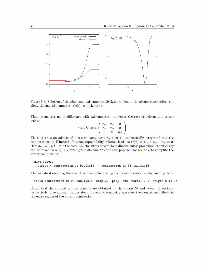
76 Rheolef version 6.6 update 17 September 2013
0
1
2
3
4
-8 -4 0 2z
u0(z, 0) axisymetriccartesian
-2
-1
0
-8 -4 0 2z
τθθ(z, 0)
Figure 5.4: Solution of the plane and axisymmetric Stokes problem in the abrupt contraction: cutalong the axis of symmetry: (left): u0; (right) τθθ.
There is another major difference with axisymmetric problems: the rate of deformation tensorwrites:
τ = 2D(u) =
τzz τrz 0τrz τrr 00 0 τθθ
Thus, there is an additional non-zero component τθθ that is automatically integrated into thecomputations in Rheolef. The incompressibility relation leads to tr(τ) = τzz + τrr + τθθ = 0.Here σtot = −p.I+ τ is the total Cauchy stress tensor (by a dimensionless procedure, the viscositycan be taken as one). By reusing the stress.cc code (see page 52) we are able to compute thetensor components:
make stress./stress < contraction-zr-P1.field > contraction-zr-P1-tau.field
The visualization along the axis of symmetry for the τθθ component is obtained by (see Fig. 5.4):
field contraction-zr-P1-tau.field -comp 22 -proj -cut -normal 0 1 -origin 0 1e-15
Recall that the τzz and τrr components are obtained by the -comp 00 and -comp 11 options,respectively. The non-zero values along the axis of symmetry expresses the elongational effects inthe entry region of the abrupt contraction.
Chapter 6
Time-dependent problems
6.1 The heat equation
Formulation
Let T > 0, Ω ⊂ Rd, d = 1, 2, 3 and fdefined in Ω. The heat problem writes:
(P ): find u, defined in Ω×]0, T [, such that
∂u
∂t−∆u = f in Ω×]0, T [,
u(0) = 0 in Ω,
u(t) = 0 on ∂Ω×]0, T [.
where f is a known function. In the present example, we consider f = 1.
Approximation
Let ∆t > 0 and tn = n∆t, n > 0. The problem is approximated with respect to time by thefollowing first-order implicit Euler scheme:
un+1 − un∆t
−∆un+1 = f(tn+1) in Ω
where un ≈ u(n∆t) and u(0) = 0. The variational formulation of the time-discretized problemwrites:(V F )n: Let un being known, find un+1 ∈ H1
0 (Ω) such that
a (un+1, v) = l(n)(v), ∀v ∈ H10 (Ω).
where
a(u, v) =
∫
Ω
(uv + ∆t∇u.∇v) v dx
l(n)(v) =
∫
Ω
(un + ∆t f(tn+1)) v dx
This is a Poisson-like problem. The discretization with respect to space of this problem is similarto those presented in section 1.1, page 15.
77
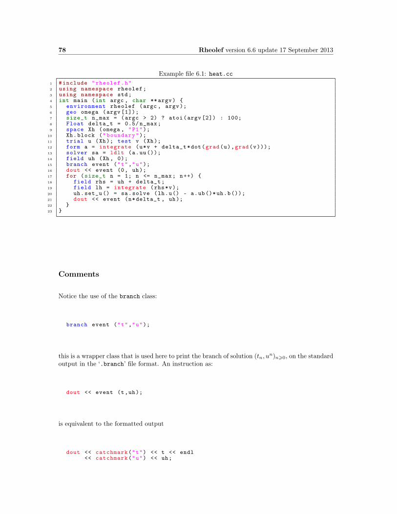
78 Rheolef version 6.6 update 17 September 2013
Example file 6.1: heat.cc1 #include "rheolef.h"2 using namespace rheolef;3 using namespace std;4 int main (int argc , char **argv) 5 environment rheolef (argc , argv);6 geo omega (argv [1]);7 size_t n_max = (argc > 2) ? atoi(argv [2]) : 100;8 Float delta_t = 0.5/ n_max;9 space Xh (omega , "P1");
10 Xh.block ("boundary");11 trial u (Xh); test v (Xh);12 form a = integrate (u*v + delta_t*dot(grad(u),grad(v)));13 solver sa = ldlt (a.uu());14 field uh (Xh, 0);15 branch event ("t","u");16 dout << event (0, uh);17 for (size_t n = 1; n <= n_max; n++) 18 field rhs = uh + delta_t;19 field lh = integrate (rhs*v);20 uh.set_u () = sa.solve (lh.u() - a.ub()*uh.b());21 dout << event (n*delta_t , uh);22 23
Comments
Notice the use of the branch class:
branch event ("t","u");
this is a wrapper class that is used here to print the branch of solution (tn, un)n>0, on the standard
output in the ‘.branch’ file format. An instruction as:
dout << event (t,uh);
is equivalent to the formatted output
dout << catchmark("t") << t << endl<< catchmark("u") << uh;
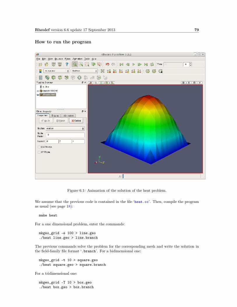
Rheolef version 6.6 update 17 September 2013 79
How to run the program
Figure 6.1: Animation of the solution of the heat problem.
We assume that the previous code is contained in the file ‘heat.cc’. Then, compile the programas usual (see page 18):
make heat
For a one dimensional problem, enter the commands:
mkgeo_grid -e 100 > line.geo./heat line.geo > line.branch
The previous commands solve the problem for the corresponding mesh and write the solution inthe field-family file format ‘.branch’. For a bidimensional one:
mkgeo_grid -t 10 > square.geo./heat square.geo > square.branch
For a tridimensional one:
mkgeo_grid -T 10 > box.geo./heat box.geo > box.branch

80 Rheolef version 6.6 update 17 September 2013
How to run the animation
branch line.branch -gnuplot -umax 0.125
A gnuplot window appears. Enter q to exit the window. For a bidimensional case, a moresophisticated procedure is required. Enter the following unix commands:
branch square.branch -paraviewparaview &
A window appears, that looks like a video player. Then, open the File->open menu andload square-..vtk. The first ’.’ stands for a wildcard, i.e. the time index family. Then,press the apply green button and, click a first time on the video play button, at the topof the window. Next, go to the object inspector window, select display and click on there-scale to data range button. Then click a second time on the video play button. An eleva-tion view can be also obtained: Select the Filter->alphabetical->wrap(scalar) menu, choose10 as scale factor and press the apply green button. Then, click on the graphic window, rotatethe view and finally re-play the animationTo generate an animation file1, go to the File->save animation menu and enter as file namesquare and as file type jpeg. A collection of jpeg files are generated by paraview. Then, runthe unix command:
ffmpeg -r 2 -i ’square.%04d.jpg’ square.mov
The animation file square.mov can now be started from any video player, such as vlc:
vlc --loop square.mov
For the tridimensional case, the animation feature is similar.
6.2 The convection-diffusion problem
Formulation
Let T > 0 and ν > 0. The convection-diffusion problem writes:
(P ): find φ, defined in Ω×]0, T [, such that
∂φ
∂t+ u.∇φ− ν∆φ+ σφ = 0 in Ω×]0, T [
φ(0) = φ0 in Ω
φ(t) = φΓ(t) on ∂Ω×]0, T [
where u, σ > 0, φ0 and φΓ being known. Notice the additional u.∇ operator.
Time approximation
This problem is approximated by the following first-order implicit Euler scheme:
φn+1 − φn Xn
∆t− ν∆φn+1 + σφn+1 = 0 in Ω
1At this time, the avi output feature is broken in paraview, and an alternate mpeg output is here suggested.
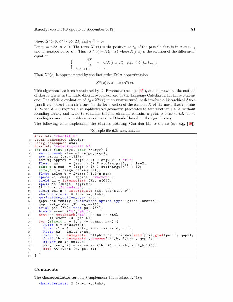
Rheolef version 6.6 update 17 September 2013 81
where ∆t > 0, φn ≈ φ(n∆t) and φ(0) = φ0.Let tn = n∆t, n > 0. The term Xn(x) is the position at tn of the particle that is in x at tn+1
and is transported by un. Thus, Xn(x) = X(tn, x) where X(t, x) is the solution of the differentialequation
dX
dt= u(X(t, x), t) p.p. t ∈ ]tn, tn+1[,
X(tn+1, x) = x.
Then Xn(x) is approximated by the first-order Euler approximation
Xn(x) ≈ x−∆tnn(x).
This algorithm has been introduced by O. Pironneau (see e.g. [35]), and is known as the methodof characteristic in the finite difference context and as the Lagrange-Galerkin in the finite elementone. The efficient evaluation of φh Xn(x) in an unstructured mesh involves a hierarchical d-tree(quadtree, octree) data structure for the localization of the element K of the mesh that containsx. When d = 3 requires also sophisticated geometric predicates to test whether x ∈ K withoutrounding errors, and avoid to conclude that no elements contains a point x close to ∂K up torounding errors. This problems is addressed in Rheolef based on the cgal library.The following code implements the classical rotating Gaussian hill test case (see e.g. [40]).
Example file 6.2: convect.cc1 #include "rheolef.h"2 using namespace rheolef;3 using namespace std;4 #include "rotating -hill.h"5 int main (int argc , char **argv) 6 environment rheolef (argc ,argv);7 geo omega (argv [1]);8 string approx = (argc > 2) ? argv [2] : "P1";9 Float nu = (argc > 3) ? atof(argv [3]) : 1e-2;
10 size_t n_max = (argc > 4) ? atoi(argv [4]) : 50;11 size_t d = omega.dimension ();12 Float delta_t = 2*acos (-1.)/ n_max;13 space Vh (omega , approx , "vector");14 field uh = interpolate (Vh, u(d));15 space Xh (omega , approx );16 Xh.block ("boundary");17 field phi_h = interpolate (Xh, phi(d,nu ,0));18 characteristic X (-delta_t*uh);19 quadrature_option_type qopt;20 qopt.set_family (quadrature_option_type :: gauss_lobatto );21 qopt.set_order (Xh.degree ());22 trial phi (Xh); test psi (Xh);23 branch event ("t","phi");24 dout << catchmark("nu") << nu << endl25 << event (0, phi_h );26 for (size_t n = 1; n <= n_max; n++) 27 Float t = n*delta_t;28 Float c1 = 1 + delta_t*phi::sigma(d,nu ,t);29 Float c2 = delta_t*nu;30 form a = integrate (c1*phi*psi + c2*dot(grad(phi),grad(psi)), qopt);31 field lh = integrate (compose(phi_h , X)*psi , qopt);32 solver sa (a.uu());33 phi_h.set_u() = sa.solve (lh.u() - a.ub()* phi_h.b());34 dout << event (t, phi_h);35 36
Comments
The characteristic variable X implements the localizer Xn(x):characteristic X (-delta_t*uh);
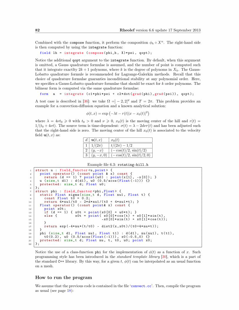
82 Rheolef version 6.6 update 17 September 2013
Combined with the compose function, it perform the composition φh Xn. The right-hand sideis then computed by using the integrate function:
field lh = integrate (compose(phi_h , X)*psi , qopt);
Notice the additional qopt argument to the integrate function. By default, when this argumentis omitted, a Gauss quadrature formulae is assumed, and the number of point is computed suchthat it integrate exactlty 2k + 1 polynoms, where k is the degree of polynoms in Xh. The Gauss-Lobatto quadrature formule is recommended for Lagrange-Galerkin methods. Recall that thischoice of quadrature formulae guaranties inconditional stability at any polynomial order. Here,we specifies a Gauss-Lobatto quadrature formulae that should be exact for k order polynoms. Thebilinear form is computed via the same quadrature formulae:
form a = integrate (c1*phi*psi + c2*dot(grad(phi),grad(psi)), qopt);
A test case is described in [36]: we take Ω =] − 2, 2[d and T = 2π. This problem provides anexample for a convection-diffusion equation and a known analytical solution:
φ(t, x) = exp(−λt− r(t)|x− x0(t)|2
)
where λ = 4νt0 > 0 with t0 > 0 and ν > 0, x0(t) is the moving center of the hill and r(t) =1/(t0 + 4νt). The source term is time-dependent: σ(t) = λ− 2dνr(t) and has been adjusted suchthat the right-hand side is zero. The moving center of the hill x0(t) is associated to the velocityfield u(t, x) as:
d u(t, x) x0(t)
1 1/(2π) t/(2π)− 1/22 (y,−x) (− cos(t)/2, sin(t)/2)3 (y,−x, 0) (− cos(t)/2, sin(t)/2, 0)
Example file 6.3: rotating-hill.h1 struct u : field_functor <u,point > 2 point operator () (const point & x) const 3 return (d == 1) ? point(u0) : point(x[1], -x[0]); 4 u (size_t d1) : d(d1), u0 (0.5/ acos(Float (-1))) 5 protected: size_t d; Float u0;6 ;7 struct phi : field_functor <phi ,Float > 8 static Float sigma(size_t d, Float nu1 , Float t) 9 const Float t0 = 0.2;
10 return 4*nu1/t0 - 2*d*nu1/(t0 + 4*nu1*t); 11 Float operator () (const point& x) const 12 point x0t;13 if (d == 1) x0t = point(x0[0] + u0*t); 14 else x0t = point( x0[0]* cos(t) + x0[1]* sin(t),15 -x0[0]* sin(t) + x0[1]* cos(t));16 17 return exp(-4*nu*(t/t0) - dist2(x,x0t )/(t0+4*nu*t));18 19 phi (size_t d1 , Float nu1 , Float t1) : d(d1), nu(nu1), t(t1),20 t0(0.2), u0 (0.5/ acos(Float (-1))), x0(-0.5,0) 21 protected: size_t d; Float nu, t, t0 , u0; point x0;22 ;
Notice the use of a class-function phi for the implementation of φ(t) as a function of x. Suchprogramming style has been introduced in the standard template library [30], which is a part ofthe standard C++ library. By this way, for a given t, φ(t) can be interpolated as an usual functionon a mesh.
How to run the program
We assume that the previous code is contained in the file ‘convect.cc’. Then, compile the programas usual (see page 18):

Rheolef version 6.6 update 17 September 2013 83
Figure 6.2: Animation of the solution of the rotating hill problem.
make convect
and enter the commands: Running the one-dimensional test case:
mkgeo_grid -e 500 -a -2 -b 2 > line2.geo./convect line2.geo P1 > line2.branchbranch line2.branch -gnuplot
Notice the hill that moves from x = −1/2 to x = 1/2. Since the exact solution is known, it ispossible to analyze the error:
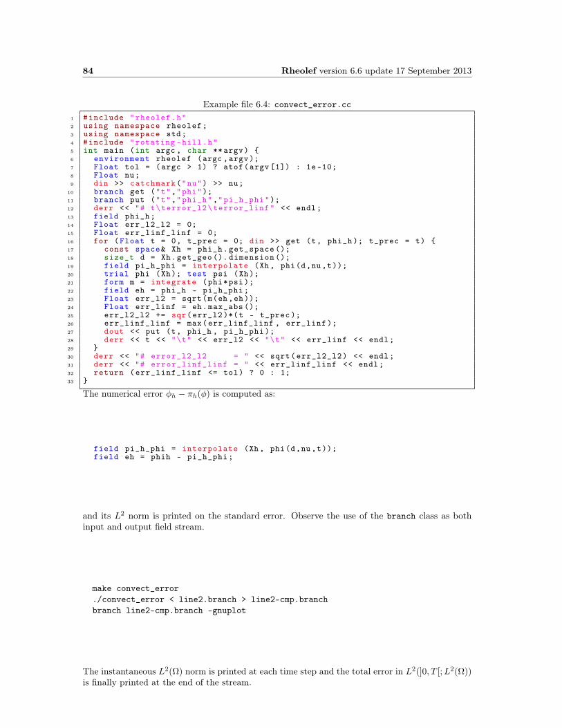
84 Rheolef version 6.6 update 17 September 2013
Example file 6.4: convect_error.cc1 #include "rheolef.h"2 using namespace rheolef;3 using namespace std;4 #include "rotating -hill.h"5 int main (int argc , char **argv) 6 environment rheolef (argc ,argv);7 Float tol = (argc > 1) ? atof(argv [1]) : 1e-10;8 Float nu;9 din >> catchmark("nu") >> nu;
10 branch get ("t","phi");11 branch put ("t","phi_h","pi_h_phi");12 derr << "# t\terror_l2\terror_linf" << endl;13 field phi_h;14 Float err_l2_l2 = 0;15 Float err_linf_linf = 0;16 for (Float t = 0, t_prec = 0; din >> get (t, phi_h ); t_prec = t) 17 const space& Xh = phi_h.get_space ();18 size_t d = Xh.get_geo (). dimension ();19 field pi_h_phi = interpolate (Xh, phi(d,nu ,t));20 trial phi (Xh); test psi (Xh);21 form m = integrate (phi*psi);22 field eh = phi_h - pi_h_phi;23 Float err_l2 = sqrt(m(eh ,eh));24 Float err_linf = eh.max_abs ();25 err_l2_l2 += sqr(err_l2 )*(t - t_prec );26 err_linf_linf = max(err_linf_linf , err_linf );27 dout << put (t, phi_h , pi_h_phi );28 derr << t << "\t" << err_l2 << "\t" << err_linf << endl;29 30 derr << "# error_l2_l2 = " << sqrt(err_l2_l2) << endl;31 derr << "# error_linf_linf = " << err_linf_linf << endl;32 return (err_linf_linf <= tol) ? 0 : 1;33
The numerical error φh − πh(φ) is computed as:
field pi_h_phi = interpolate (Xh, phi(d,nu ,t));field eh = phih - pi_h_phi;
and its L2 norm is printed on the standard error. Observe the use of the branch class as bothinput and output field stream.
make convect_error./convect_error < line2.branch > line2-cmp.branchbranch line2-cmp.branch -gnuplot
The instantaneous L2(Ω) norm is printed at each time step and the total error in L2(]0, T [;L2(Ω))is finally printed at the end of the stream.

Rheolef version 6.6 update 17 September 2013 85
‖φh − πh(φ)‖L2(L2) ‖φh − πh(φ)‖L∞(L∞)
0.001
0.01
0.1
1
0.001 0.01 0.1 1
h
∆t = 2π/50∆t = 2π/100∆t = 2π/200
22
P1P2
0.001
0.01
0.1
1
0.001 0.01 0.1 1
h
∆t = 2π/50∆t = 2π/100∆t = 2π/200
P1P2
Figure 6.3: Diffusion-convection when d = 1 and ν = 10−2: convergence versus h and ∆t for P1
and P2 elements: (left) in L2(L2) norm; (right) in L∞(L∞) norm.
A P2 approximation can be used as well:
./convect line2.geo P2 > line2.branchbranch line2.branch -gnuplot./convect_error < line2.branch > line2-cmp.branch
On Fig. 6.3.left we observe the L2(L2) convergence versus h for the P1 and P2 elements whend = 1: the errors reaches a plateau that decreases versus ∆t. On Fig. 6.3.right the L∞(L∞) normof the error presents a similar behavior. Since the plateau are equispaced, the convergence versus∆t is of first order.These computation was performed for a convection-diffusion problem with ν = 10−2. The puretransport problem (ν = 0, without diffusion) computation is obtained by:
./convect line2.geo P1 0 > line2.branchbranch line2.branch -gnuplot
Let us turn to the two-dimensional test case:
mkgeo_grid -t 80 -a -2 -b 2 -c -2 -d 2 > square2.geo./convect square2.geo P1 > square2.branchbranch square2.branch -paraviewparaview &
The visualization and animation are similar to those of the head problem previously presentedin paragraph 6.1. Observe the rotating hill. The result is shown on Fig. 6.2. The error analysiswrites:
./convect_error < square2.branch > square2-cmp.branchbranch square2-cmp.branch -paraview
From the paraview menu, you can visualize simultaneously both the approximate solution and theLagrange interpolate of the exact one. Finally, the three-dimensional case:
mkgeo_grid -T 15 -a -2 -b 2 -c -2 -d 2 -f -2 -g 2 > cube2.geo./convect cube2.geo P1 > cube2.branch
The visualization is similar to the two-dimensional case.

86 Rheolef version 6.6 update 17 September 2013
6.3 The Navier-Stokes problem
Formulation
This longer example combines most functionalities presented in the previous examples.Let us consider the Navier-Stokes problem for the driven cavity in Ω =]0, 1[d, d = 2, 3. Let Re > 0be the Reynolds number, and T > 0 a final time. The problem writes:
(NS): find u = (u0, . . . , ud−1) and p defined in Ω×]0, T [ such that:
Re
(∂u
∂t+ u.∇u
)− div(2D(u)) + ∇p = 0 in Ω×]0, T [,
− divu = 0 in Ω×]0, T [,u(t=0) = 0 in Ω× 0, T,
u = (1, 0) on Γtop×]0, T [,u = 0 on (Γleft ∪ Γright ∪ Γbottom)×]0, T [,∂u0
∂n=
∂u1
∂n= u2 = 0 on (Γback ∪ Γfront)×]0, T [ when d = 3,
where D(u) = (∇u + ∇uT )/2. This nonlinear problem is the natural extension of the linearStokes problem, as presented in paragraph 6.3, page 86. The boundaries are represented onFig. 4.1, page 48.
Time approximation
Let ∆t > 0. Let us consider the following backward second order scheme, for all φ ∈ C2([0, T ]) :
dφ
dt(t) =
3φ(t)− 4φ(t−∆t) + φ(t− 2∆t)
2∆t+O(∆t2)
The problem is approximated by the following second-order implicit scheme (BDF2):
Re3un+1 − 4un Xn + un−1 Xn−1
2∆t− div(2D(un+1)) + ∇pn+1 = 0 in Ω,
− divun+1 = 0 in Ω,un+1 = (1, 0) on Γtop,un+1 = 0 on Γleft ∪ Γright ∪ Γbottom,
∂un+10
∂n=∂un+1
1
∂n= un+1
2 = 0 on Γback ∪ Γfront when d = 3,
where, following [7, 15]:
Xn(x) = x−∆tu∗(x)
Xn−1(x) = x− 2∆tu∗(x)
u∗ = 2un − un−1
It is a second order extension of the method previously introduced in paragraph 6.2 page 80. Thescheme defines a second order recurrence for the sequence (un)n>−1, that starts with u−1 = u0 = 0.
Variational formulation
The variational formulation of this problem expresses:(NS)∆t: find un+1 ∈ V(1) and pn+1 ∈ L2
0(Ω) such that:
a(un+1,v) + b(v, pn+1) = m(fn,v), ∀v ∈ V(0),
b(un+1, q) = 0, ∀q ∈ L20(Ω),
Rheolef version 6.6 update 17 September 2013 87
where
fn =Re
2∆t
(4un Xn − un−1 Xn
)
and
a(u,v) =3Re
2∆t
∫
Ω
u.v dx+
∫
Ω
2D(u) : D(v) dx
and b(., .) and V(α) was already introduced in paragraph 4.4, page 57, while studying the Stokesproblem.
Space approximation
The Taylor-Hood [22] finite element approximation of this generalized Stokes problem was alsoconsidered in paragraph 4.4, page 57. We introduce a mesh Th of Ω and the finite dimensionalspaces Xh, Vh(α) and Qh. The approximate problem writes:
(NS)∆t,h: find un+1h ∈ Vh(1) and pn+1 ∈ Qh such that:
a(un+1h ,v) + b(v, pn+1
h ) = m(fnh ,v), ∀v ∈ Vh(0),b(un+1
h , q) = 0, ∀q ∈ Qh.(6.1)
where
fnh =Re
2∆t
(4unh Xn − un−1
h Xn)
The problem reduces to a sequence resolution of a generalized Stokes problems.

88 Rheolef version 6.6 update 17 September 2013
Example file 6.5: navier_stokes_solve.icc1 using namespace std;2 int navier_stokes_solve (3 Float Re , Float delta_t , field l0h , field& uh, field& ph,4 size_t& max_iter , Float& tol , odiststream *p_derr =0) 5 const space& Xh = uh.get_space ();6 const space& Qh = ph.get_space ();7 string label = "navier -stokes -" + Xh.get_geo (). name ();8 quadrature_option_type qopt;9 qopt.set_family(quadrature_option_type :: gauss_lobatto );
10 qopt.set_order(Xh.degree ());11 trial u (Xh), p (Qh);12 test v (Xh), q (Qh);13 form mp = integrate (p*q, qopt);14 form m = integrate (dot(u,v), qopt);15 form a = integrate (2* ddot(D(u),D(v)) + 1.5*(Re/delta_t )*dot(u,v), qopt);16 form b = integrate (-div(u)*q, qopt);17 solver sa (a.uu());18 solver_abtb stokes (a.uu(), b.uu(), mp.uu());19 if (p_derr != 0) *p_derr << "[" << label << "] #n |du/dt|" << endl;20 field uh1 = uh;21 for (size_t n = 0; true; n++) 22 field uh2 = uh1;23 uh1 = uh;24 field uh_star = 2.0* uh1 - uh2;25 characteristic X1 ( -delta_t*uh_star );26 characteristic X2 (-2.0* delta_t*uh_star );27 field l1h = integrate (dot(compose(uh1 ,X1),v), qopt);28 field l2h = integrate (dot(compose(uh2 ,X2),v), qopt);29 field lh = l0h + (Re/delta_t )*(2* l1h - 0.5* l2h);30 stokes.solve (lh.u() - a.ub()*uh.b(), -(b.ub()*uh.b()),31 uh.set_u(), ph.set_u ());32 field duh_dt = (3*uh - 4*uh1 + uh2 )/(2* delta_t );33 Float residual = sqrt(m(duh_dt ,duh_dt ));34 if (p_derr != 0) *p_derr << "[" << label << "] "<< n << " " << residual << endl;35 if (residual < tol) 36 tol = residual;37 max_iter = n;38 return 0;39 40 if (n == max_iter -1) 41 tol = residual;42 return 1;43 44 45
Comments
The navier_stokes_solve function is similar to the ‘stokes_cavity.cc’. It solves here a gen-eralized Stokes problem and manages a right-hand side fh:
characteristic X1 ( -delta_t*uh_star );characteristic X2 (-2.0* delta_t*uh_star );field l1h = integrate (compose(uh1 ,X1)*v, qopt);field l2h = integrate (compose(uh2 ,X2)*v, qopt);field lh = l0h + (Re/delta_t )*(2* l1h - 0.5* l2h);
This last computation is similar to those done in the ‘convect.cc’ example. The generalizedStokes problem is solved by the solver_abtb class. The stopping criterion is related to thestationary solution or the maximal iteration number.
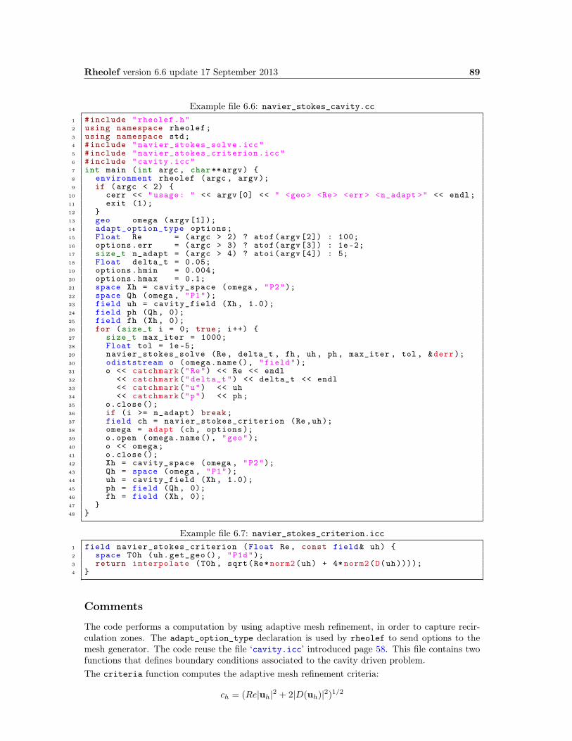
Rheolef version 6.6 update 17 September 2013 89
Example file 6.6: navier_stokes_cavity.cc1 #include "rheolef.h"2 using namespace rheolef;3 using namespace std;4 #include "navier_stokes_solve.icc"5 #include "navier_stokes_criterion.icc"6 #include "cavity.icc"7 int main (int argc , char**argv) 8 environment rheolef (argc , argv);9 if (argc < 2)
10 cerr << "usage: " << argv [0] << " <geo > <Re > <err > <n_adapt >" << endl;11 exit (1);12 13 geo omega (argv [1]);14 adapt_option_type options;15 Float Re = (argc > 2) ? atof(argv [2]) : 100;16 options.err = (argc > 3) ? atof(argv [3]) : 1e-2;17 size_t n_adapt = (argc > 4) ? atoi(argv [4]) : 5;18 Float delta_t = 0.05;19 options.hmin = 0.004;20 options.hmax = 0.1;21 space Xh = cavity_space (omega , "P2");22 space Qh (omega , "P1");23 field uh = cavity_field (Xh, 1.0);24 field ph (Qh, 0);25 field fh (Xh, 0);26 for (size_t i = 0; true; i++) 27 size_t max_iter = 1000;28 Float tol = 1e-5;29 navier_stokes_solve (Re , delta_t , fh , uh, ph, max_iter , tol , &derr);30 odiststream o (omega.name(), "field");31 o << catchmark("Re") << Re << endl32 << catchmark("delta_t") << delta_t << endl33 << catchmark("u") << uh34 << catchmark("p") << ph;35 o.close ();36 if (i >= n_adapt) break;37 field ch = navier_stokes_criterion (Re ,uh);38 omega = adapt (ch , options );39 o.open (omega.name(), "geo");40 o << omega;41 o.close ();42 Xh = cavity_space (omega , "P2");43 Qh = space (omega , "P1");44 uh = cavity_field (Xh, 1.0);45 ph = field (Qh , 0);46 fh = field (Xh , 0);47 48
Example file 6.7: navier_stokes_criterion.icc1 field navier_stokes_criterion (Float Re , const field& uh) 2 space T0h (uh.get_geo(), "P1d");3 return interpolate (T0h , sqrt(Re*norm2(uh) + 4* norm2(D(uh))));4
Comments
The code performs a computation by using adaptive mesh refinement, in order to capture recir-culation zones. The adapt_option_type declaration is used by rheolef to send options to themesh generator. The code reuse the file ‘cavity.icc’ introduced page 58. This file contains twofunctions that defines boundary conditions associated to the cavity driven problem.The criteria function computes the adaptive mesh refinement criteria:
ch = (Re|uh|2 + 2|D(uh)|2)1/2
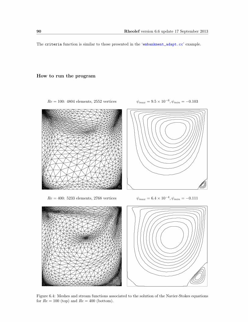
90 Rheolef version 6.6 update 17 September 2013
The criteria function is similar to those presented in the ‘embankment_adapt.cc’ example.
How to run the program
Re = 100: 4804 elements, 2552 vertices ψmax = 9.5× 10⁻⁶, ψmin = −0.103
Re = 400: 5233 elements, 2768 vertices ψmax = 6.4× 10⁻⁴, ψmin = −0.111
Figure 6.4: Meshes and stream functions associated to the solution of the Navier-Stokes equationsfor Re = 100 (top) and Re = 400 (bottom).

Rheolef version 6.6 update 17 September 2013 91
Re = 1000: 5873 elements, 3106 vertices ψmax = 1.64× 10⁻³, ψmin = −0.117
Figure 6.5: Meshes and stream functions associated to the solution of the Navier-Stokes equationsfor Re = 1000.
The mesh loop adaptation is initiated from a bamg mesh (see also appendix B.1).
bamg -g square.bamgcad -o square.bamgbamg2geo square.bamg square.dmn > square.geo
Then, compile and run the Navier-Stokes solver for the driven cavity for Re = 100:
make navier_stokes_cavity./navier_stokes_cavity square.geo 100
The program performs a computation with Re = 100. By default the time step is ∆t = 0.05and the computation loops for five mesh adaptations. At each time step, the program prints anapproximation of the time derivative, and stops when a stationary solution is reached. Then, wevisualize the ‘square-5.geo’ adapted mesh and its associated solution:
geo square-5.geofield square-5.field.gz -velocity -scale 4 -mayavi
Notice the -scale option that applies a multiplicative factor to the arrow length when plotting.The representation of the stream function writes:
make streamf_cavityzcat square-5.field.gz | ./streamf_cavity | field -bw -n-iso-negative 10 -
The programs ‘streamf_cavity.cc’, already introduced page 63, is here reused. The last optionsof the field program draws isocontours of the stream function using lines, as shown on Fig. 6.4.The zero isovalue separates the main flow from recirculations, located in corners at the bottom ofthe cavity.For Re = 400 and 1000 the computation writes:
./navier_stokes_cavity square.geo 400
./navier_stokes_cavity square.geo 1000
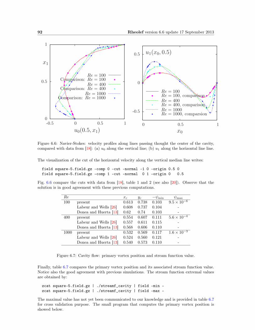
92 Rheolef version 6.6 update 17 September 2013
0
0.5
1
-0.5 0 0.5 1
u0(0.5, x1)
x1
Re = 100Comparison: Re = 100
Re = 400Comparison: Re = 400
Re = 1000Comparison: Re = 1000
-0.5
0
0.5
0 0.5 1x0
u1(x0, 0.5)
Re = 100Re = 100, comparisonRe = 400Re = 400, comparisonRe = 1000Re = 1000, comparsion
Figure 6.6: Navier-Stokes: velocity profiles along lines passing thought the center of the cavity,compared with data from [18]: (a) u0 along the vertical line; (b) u1 along the horizontal line line.
The visualization of the cut of the horizontal velocity along the vertical median line writes:
field square-5.field.gz -comp 0 -cut -normal -1 0 -origin 0.5 0field square-5.field.gz -comp 1 -cut -normal 0 1 -origin 0 0.5
Fig. 6.6 compare the cuts with data from [18], table 1 and 2 (see also [20]). Observe that thesolution is in good agreement with these previous computations.
Re xc yc −ψmin ψmax
100 present 0.613 0.738 0.103 9.5× 10⁻⁶
Labeur and Wells [26] 0.608 0.737 0.104 -Donea and Huerta [13] 0.62 0.74 0.103 -
400 present 0.554 0.607 0.111 5.6× 10⁻⁴
Labeur and Wells [26] 0.557 0.611 0.115 -Donea and Huerta [13] 0.568 0.606 0.110 -
1000 present 0.532 0.569 0.117 1.6× 10⁻³
Labeur and Wells [26] 0.524 0.560 0.121 -Donea and Huerta [13] 0.540 0.573 0.110 -
Figure 6.7: Cavity flow: primary vortex position and stream function value.
Finally, table 6.7 compares the primary vortex position and its associated stream function value.Notice also the good agreement with previous simulations. The stream function extremal valuesare obtained by:
zcat square-5.field.gz | ./streamf_cavity | field -min -zcat square-5.field.gz | ./streamf_cavity | field -max -
The maximal value has not yet been communicated to our knowledge and is provided in table 6.7for cross validation purpose. The small program that computes the primary vortex position isshowed below.

Rheolef version 6.6 update 17 September 2013 93
make vortex_positionzcat square-5.field.gz | ./streamf_cavity | ./vortex_position
Example file 6.8: vortex_position.cc1 #include "rheolef.h"2 using namespace rheolef;3 int main (int argc , char** argv) 4 environment rheolef (argc , argv);5 check_macro (communicator (). size() == 1, "please , use sequentially");6 field psi_h;7 din >> psi_h;8 size_t idof_min = 0;9 Float psi_min = std:: numeric_limits <Float >:: max ();
10 for (size_t idof = 0, ndof = psi_h.ndof (); idof < ndof; idof ++) 11 if (psi_h.dof(idof) >= psi_min) continue;12 psi_min = psi_h.dof(idof);13 idof_min = idof;14 15 const array <point >& xdof = psi_h.get_space (). get_xdofs ();16 point xmin = xdof [idof_min ];17 dout << "xc\t\tyc\t\tpsi" << std::endl18 << xmin [0] << "\t" << xmin [1] << "\t" << psi_min << std::endl;19
For higher Reynolds number, Shen [47] showed in 1991 that the flow converges to a stationary statefor Reynolds numbers up to 10 000; for Reynolds numbers larger than a critical value 10 000 <Re1 < 10 500 and less than another critical value 15 000 < Re2 < 16 000, these authors foundedthat the flow becomes periodic in time which indicates a Hopf bifurcation; the flow loses timeperiodicity for Re ≥ Re2. In 1998, Ould Salihi [33] founded a loss of stationarity between 10 000and 20 000. In 2002, Auteri et al. [4] estimated the critical value for the apparition of the firstinstability to Re1 ≈ 8018. In 2005, Erturk et al. [14] computed steady driven cavity solutions upto Re 6 21 000. Also in 2005, this result was infirmed by [16]: these authors estimated Re1 closeto 8000, in agreement with [4]. The 3D driven cavity has been investigated in [28] by the methodof characteristic (see also [27] for 3D driven cavity computations). In conclusion, the explorationof the driven cavity at large Reynolds number is a fundamental challenge in computational fluiddynamics.

94 Rheolef version 6.6 update 17 September 2013

Part III
Advanced and highly nonlinearproblems
95

Chapter 7
Equation defined on a surface
This chapter deals with equations defined on a closed hypersurface. We present three differentnumerical methods: the direct resolution of the problem on an explicit surface mesh generatedindependently of Rheolef, the direct resolution on a surface mesh generated by Rheolef from avolume mesh, and finally a level set type method based on a volume mesh in an h-narrow bandcontaining the surface. This last method allows to define hybrid operators between surface andvolume-based finite element fields. These methods are demonstrated on two model problems andtwo different surfaces.Let us consider a closed surface Γ ∈ Rd, d = 2 or 3 and Γ is a connected C2 surface of dimensiond− 1 with ∂Γ = 0. We first consider the following problem:
(P1) find u, defined on Γ such that:
u−∆su = f on Γ (7.1)
where f ∈ L2(Γ). For all function u defined on Γ, ∆s denotes the Laplace-Beltrami operator:
∆su = divs(∇su)
where ∇s and divs are the tangential derivative and the surface divergence along Γ, definedrespectively, for all scalar field ϕ and vector field v by:
∇sϕ = (I − n⊗ n)∇ϕdivs v = (I − n⊗ n) : ∇v
Here, n denotes a unit normal on Γ.We also consider the following variant of this problem:
(P2) find u, defined on Γ such that:
−∆su = f on Γ (7.2)
This second problem is similar to the first one: the Helmholtz operator I −∆s has been replacedby the Laplace-Beltrami one −∆s. In that case, the solution is defined up to a constant: if u isa solution, then u + c is also a solution for any constant c ∈ R. Thus, we refers to (P1) as theHelmholtz-Beltrami problem and to (P2) as the Laplace-Beltrami one.
7.1 Approximation on an explicit surface mesh
The Helmholtz-Beltrami problem
Tanks to the surface Green formula (see appendix A.3), the variational formulation of problem(P1) writes:
97
98 Rheolef version 6.6 update 17 September 2013
(V F1): find u ∈ H1(Γ) such that:
a(u, v) = l(v), ∀v ∈ H1(Γ)
where for all u, v ∈ H1(Γ),
a(u, v) =
∫
Γ
(u v +∇su.∇sv) ds
l(v) =
∫
Γ
f v ds
Let k > 1 and consider a k-th order curved surface finite element mesh Γh of Γ. We define thespace Wh:
Wh =vh ∈ H1(Γh); v|S ∈ Pk,∀S ∈ Γh
The approximate problem writes:(V F1)h: find uh ∈Wh such that:
a(uh, vh) = l(vh), ∀vh ∈Wh
Example file 7.1: helmholtz_s.cc1 #include "rheolef.h"2 using namespace rheolef;3 using namespace std;4 #include "sphere.icc"5 int main(int argc , char**argv) 6 environment rheolef(argc , argv);7 geo gamma (argv [1]);8 size_t d = gamma.dimension ();9 space Wh (gamma , argv [2]);
10 trial u (Wh); test v (Wh);11 form a = integrate (u*v + dot(grad_s(u),grad_s(v)));12 field lh = integrate (f(d)*v);13 field uh (Wh);14 solver sa (a.uu());15 uh.set_u () = sa.solve (lh.u() - a.ub()*uh.b());16 dout << uh;17
Comments
The problem involves the Helmholtz operator and thus, the code is similar to ‘neumann-nh.cc’presented page 32. Let us comments the only differences:
form a = integrate (u*v + dot(grad_s(u),grad_s(v)));
The form refers to the grad_s operator instead of the grad one, since only the coordinates relatedto the surface are involved.
field lh = integrate (f(d)*v);
The right-hand-side does not involve any boundary term, since the surface Γ is closed: the bound-ary domain ∂Γ = ∅. As test problem, the surface Γ is the unit circle when d = 2 and the unitsphere when d = 3. The data f has been chosen as in [11, p. 17]. This choice is convenient sincethe exact solution is known. Recall that the spherical coordinates (ρ, θ, φ) are defined from theartesian ones (x0, x1, x2) by:
ρ =√x2
0 + x21 + x2
2, φ = arccos (x2/ρ) , θ =
arccos(x0/√x2
0 + x21
)when x1 > 0
2π − arccos(x0/√x2
0 + x21
)otherwise
Rheolef version 6.6 update 17 September 2013 99
Example file 7.2: sphere.icc1 struct p : field_functor <p,Float > 2 Float operator () (const point& x) const 3 if (d == 2) return 26*( pow(x[0] ,5) - 10*pow(x[0] ,3)* sqr(x[1])4 + 5*x[0]* pow(x[1] ,4));5 else return 3*sqr(x[0])*x[1] - pow(x[1] ,3);6 7 p (size_t d1) : d(d1) 8 protected: size_t d;9 ;
10 struct f : field_functor <f,Float > 11 Float operator () (const point& x) const 12 if (d == 2) return _p(x)/pow(norm(x),5);13 else return alpha*_p(x);14 15 f (size_t d1) : d(d1), _p(d1) 16 Float pi = acos(Float (-1));17 alpha = -(13./8.)* sqrt (35./pi);18 19 protected: size_t d; p _p; Float alpha;20 ;21 struct u_exact : field_functor <u_exact ,Float > 22 Float operator () (const point& x) const 23 if (d == 2) return _f(x)/(25+ sqr(norm(x)));24 else return sqr(norm(x))/(12+ sqr(norm(x)))*_f(x);25 26 u_exact (size_t d1) : d(d1), _f(d1) 27 protected: size_t d; f _f;28 ;29 Float phi (const point& x) return norm(x) - 1;
How to run the program
The program compile as usual:
make helmholtz_s
A mesh of a circle is generated by:
mkgeo_ball -s -e 100 > circle.geogeo circle -mayavi
The mkgeo_ball is a convenient script that generates a mesh with the gmsh mesh generator. Then,the problem resolution writes:
./helmholtz_s circle P1 > circle.fieldfield circle.field -mayavifield circle.field -mayavi -elevation
The tridimensional case is similar:
mkgeo_ball -s -t 10 > sphere.geogeo sphere.geo -mayavi -stereo./helmholtz_s sphere.geo P1 > sphere.fieldfield sphere.field -mayavi -stereo
The solution is represented on Fig .7.1.left.

100 Rheolef version 6.6 update 17 September 2013
Figure 7.1: Helmholtz-Beltrami problem: high-order curved surface mesh and its correspondingisoparametric solution: (top) order = 1; (bottom) order = 3.
Higher-order isoparametric finite elements can be considered for the curved geometry:
mkgeo_ball -s -e 30 -order 3 > circle-P3.geogeo circle-P3.geo -subdivide 10
Observe the curved edges (see Fig .7.1). The -subdivide option allows a graphical representationof the curved edges by subdividing each edge in ten linear parts, since graphical softwares are notyet able to represent curved elements. The computation with the P3 isoparametric approximationwrites:
./helmholtz_s circle-P3 P3 > circle-P3.fieldfield circle-P3.field -mayavi -elevation
Notice that both the curved geometry and the finite element are second order. The tridimensionalcounterpart writes simply:
mkgeo_ball -s -t 10 -order 3 > sphere-P3.geogeo sphere-P3.geo./helmholtz_s sphere-P3 P3 > sphere-P3.fieldfield sphere-P3.field -mayavi -stereo
Rheolef version 6.6 update 17 September 2013 101
The solution is represented on Fig .7.1).right-bottom. The graphical representation is not yet ableto represent the high-order approximation: each elements is subdivided and a piecewise linearrepresentation is used in each sub-elements.Since the exact solution is known, the error can be computed: this is done by the programhelmholtz_s_error.cc. This file is not presented here, as it is similar to some others examples,but can be founded in the Rheolef example directory. Figure 7.2 plots the error in various normsversus element size for different isoparametric approximations.
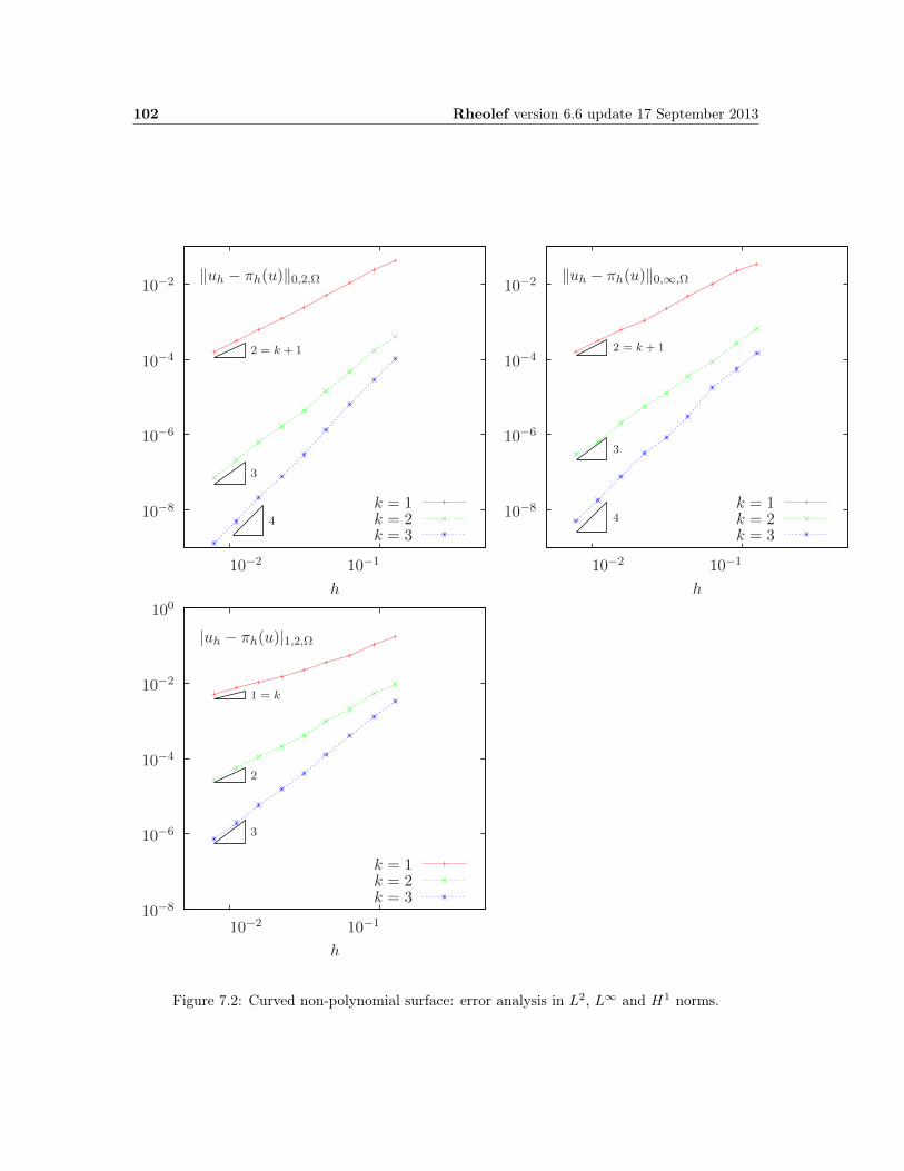
102 Rheolef version 6.6 update 17 September 2013
10−8
10−6
10−4
10−2
10−2 10−1
h
‖uh − πh(u)‖0,2,Ω
2 = k + 1
3
4
k = 1k = 2k = 3
10−8
10−6
10−4
10−2
10−2 10−1
h
‖uh − πh(u)‖0,∞,Ω
2 = k + 1
3
4k = 1k = 2k = 3
10−8
10−6
10−4
10−2
100
10−2 10−1
h
|uh − πh(u)|1,2,Ω
1 = k
2
3
k = 1k = 2k = 3
Figure 7.2: Curved non-polynomial surface: error analysis in L2, L∞ and H1 norms.
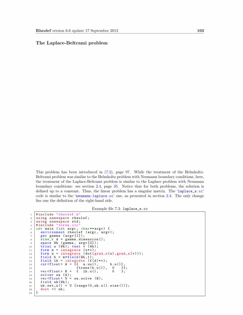
Rheolef version 6.6 update 17 September 2013 103
The Laplace-Beltrami problem
This problem has been introduced in (7.2), page 97. While the treatment of the Helmholtz-Beltrami problem was similar to the Helmholtz problem with Neumann boundary conditions, here,the treatment of the Laplace-Beltrami problem is similar to the Laplace problem with Neumannboundary conditions: see section 2.4, page 35. Notice that for both problems, the solution isdefined up to a constant. Thus, the linear problem has a singular matrix. The ‘laplace_s.cc’code is similar to the ‘neumann-laplace.cc’ one, as presented in section 2.4. The only changelies one the definition of the right-hand side.
Example file 7.3: laplace_s.cc1 #include "rheolef.h"2 using namespace rheolef;3 using namespace std;4 #include "torus.icc"5 int main (int argc , char**argv) 6 environment rheolef (argc , argv);7 geo gamma (argv [1]);8 size_t d = gamma.dimension ();9 space Wh (gamma , argv [2]);
10 trial u (Wh); test v (Wh);11 form m = integrate (u*v);12 form a = integrate (dot(grad_s(u),grad_s(v)));13 field b = m*field(Wh ,1);14 field lh = integrate (f(d)*v);15 csr <Float > A = a.uu(), b.u(),16 trans(b.u()), 0 ;17 vec <Float > B = lh.u(), 0 ;18 solver sa (A);19 vec <Float > U = sa.solve (B);20 field uh(Wh);21 uh.set_u () = U [range(0,uh.u(). size ())];22 dout << uh;23
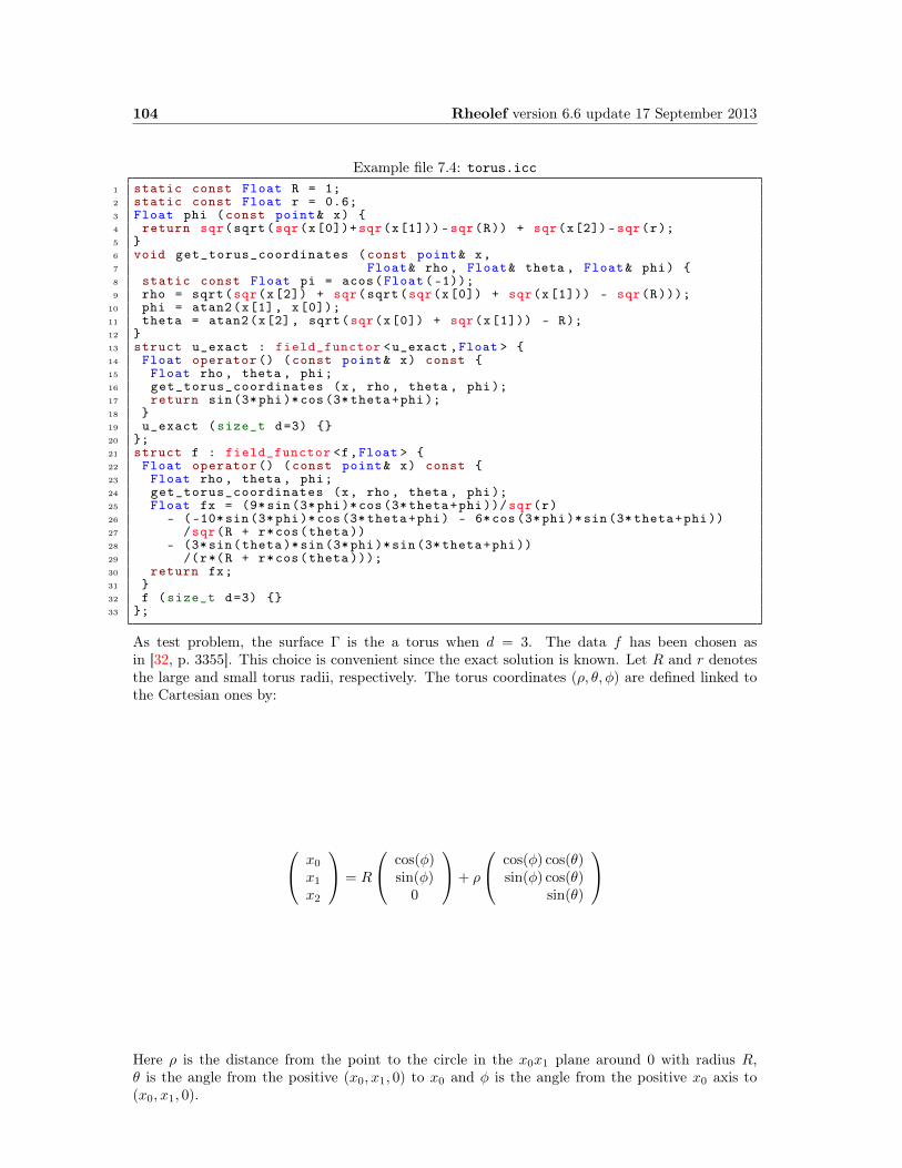
104 Rheolef version 6.6 update 17 September 2013
Example file 7.4: torus.icc1 static const Float R = 1;2 static const Float r = 0.6;3 Float phi (const point& x) 4 return sqr(sqrt(sqr(x[0])+ sqr(x[1]))- sqr(R)) + sqr(x[2])-sqr(r);5 6 void get_torus_coordinates (const point& x,7 Float& rho , Float& theta , Float& phi) 8 static const Float pi = acos(Float (-1));9 rho = sqrt(sqr(x[2]) + sqr(sqrt(sqr(x[0]) + sqr(x[1])) - sqr(R)));
10 phi = atan2(x[1], x[0]);11 theta = atan2(x[2], sqrt(sqr(x[0]) + sqr(x[1])) - R);12 13 struct u_exact : field_functor <u_exact ,Float > 14 Float operator () (const point& x) const 15 Float rho , theta , phi;16 get_torus_coordinates (x, rho , theta , phi);17 return sin(3*phi)*cos (3* theta+phi);18 19 u_exact (size_t d=3) 20 ;21 struct f : field_functor <f,Float > 22 Float operator () (const point& x) const 23 Float rho , theta , phi;24 get_torus_coordinates (x, rho , theta , phi);25 Float fx = (9*sin(3*phi)*cos (3* theta+phi))/ sqr(r)26 - (-10*sin(3*phi)*cos (3* theta+phi) - 6*cos(3*phi)*sin (3* theta+phi))27 /sqr(R + r*cos(theta))28 - (3*sin(theta)*sin (3* phi)*sin(3* theta+phi))29 /(r*(R + r*cos(theta )));30 return fx;31 32 f (size_t d=3) 33 ;
As test problem, the surface Γ is the a torus when d = 3. The data f has been chosen asin [32, p. 3355]. This choice is convenient since the exact solution is known. Let R and r denotesthe large and small torus radii, respectively. The torus coordinates (ρ, θ, φ) are defined linked tothe Cartesian ones by:
x0
x1
x2
= R
cos(φ)sin(φ)
0
+ ρ
cos(φ) cos(θ)sin(φ) cos(θ)
sin(θ)
Here ρ is the distance from the point to the circle in the x0x1 plane around 0 with radius R,θ is the angle from the positive (x0, x1, 0) to x0 and φ is the angle from the positive x0 axis to(x0, x1, 0).
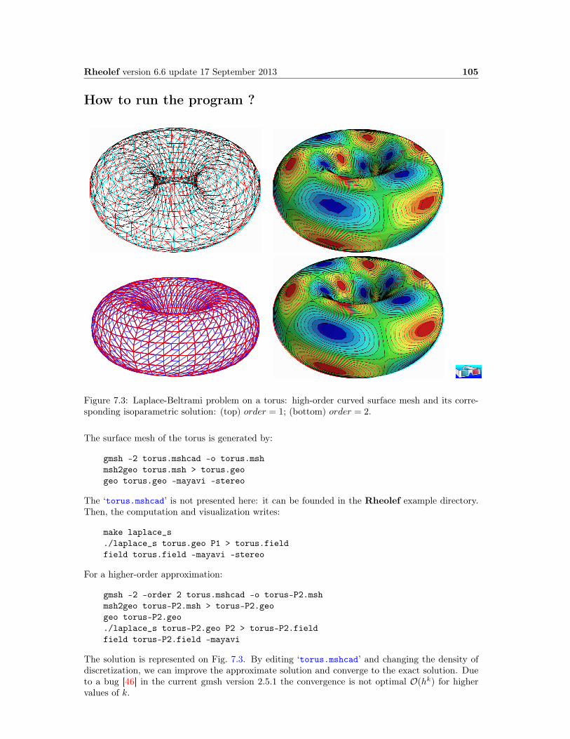
Rheolef version 6.6 update 17 September 2013 105
How to run the program ?
Figure 7.3: Laplace-Beltrami problem on a torus: high-order curved surface mesh and its corre-sponding isoparametric solution: (top) order = 1; (bottom) order = 2.
The surface mesh of the torus is generated by:
gmsh -2 torus.mshcad -o torus.mshmsh2geo torus.msh > torus.geogeo torus.geo -mayavi -stereo
The ‘torus.mshcad’ is not presented here: it can be founded in the Rheolef example directory.Then, the computation and visualization writes:
make laplace_s./laplace_s torus.geo P1 > torus.fieldfield torus.field -mayavi -stereo
For a higher-order approximation:
gmsh -2 -order 2 torus.mshcad -o torus-P2.mshmsh2geo torus-P2.msh > torus-P2.geogeo torus-P2.geo./laplace_s torus-P2.geo P2 > torus-P2.fieldfield torus-P2.field -mayavi
The solution is represented on Fig. 7.3. By editing ‘torus.mshcad’ and changing the density ofdiscretization, we can improve the approximate solution and converge to the exact solution. Dueto a bug [46] in the current gmsh version 2.5.1 the convergence is not optimal O(hk) for highervalues of k.
106 Rheolef version 6.6 update 17 September 2013
7.2 Building a surface mesh from a level set function
The previous method is limited to not-too-complex surface Γ, that can be described by a regularfinite element surface mesh Γh. When the surface change, as in a time-dependent process, complexchange of topology often occurs and the mesh Γh can degenerate or be too complex to be efficientlymeshed. In that case, the surface is described implicitly as the zero isosurface, or zero level set, ofa function:
Γ = x ∈ Λ; φ(x) = 0where Λ ⊂ Rd is a bounding box of the surface Γ.The following code automatically generates the mesh Γh of the surface described by the zeroisosurface of a discrete φh ∈ Xh level set function:
Γh = x ∈ Λ; φh(x) = 0
where Xh is a piecewise affine functional space over a mesh Th of Λ:
Xh = ϕ ∈ L2(Λ) ∩ C0(Λ); ϕ/K ∈ P1, ∀K ∈ Th
The polynomial approximation is actually limited here to first order: building higher order curvedfinite element surface meshes from a level set function is planed for the future versions of Rheolef.Finally, a computation, as performed in the previous paragraph can be done using Γh. We alsopoint out the limitations of this approach.
Example file 7.5: level_set_sphere.cc1 #include "rheolef.h"2 using namespace rheolef;3 using namespace std;4 #include "sphere.icc"5 int main (int argc , char**argv) 6 environment rheolef (argc ,argv);7 geo lambda (argv [1]);8 level_set_option_type opts;9 opts.split_to_triangle
10 = (argc > 2 && argv [2] == std:: string("-tq")) ? false : true;11 space Xh (lambda , "P1");12 field phi_h = interpolate(Xh, phi);13 geo gamma = level_set (phi_h , opts);14 dout << gamma;15
Comments
All the difficult work of building the intersection mesh Γh, defined as the zero level set of the φhfunction, is performed by the level_set function:
geo gamma = level_set (phi_h , opts);
When d = 3, intersected tetrahedra leads to either triangular or quadrangular faces. By default,quadrangular faces are split into two triangles. An optional -tq program flag allows to conservequadrangles in the surface mesh: it set the split_to_triangle optional field to false.
How to run the program ?
After the compilation, generates the mesh of a bounding box Λ = [−2, 2]d of the surface and runthe program:
Rheolef version 6.6 update 17 September 2013 107
make level_set_spheremkgeo_grid -t 20 -a -2 -b 2 -c -2 -d 2 > square2.geo./level_set_sphere square2.geo > circle.geogeo circle.geo -mayavi -stereo
The computation of the previous paragraph can be reused:
./helmholtz_s circle.geo P1 | field -mayavi -stereo -
Notice that, while the bounding box mesh was uniform, the intersected mesh could present arbi-trarily small edge length (see also Fig. 7.4):
geo -min-element-measure circle.geogeo -max-element-measure circle.geo
Let us turn to the d = 3 case:
mkgeo_grid -T 20 -a -2 -b 2 -c -2 -d 2 -f -2 -g 2 > cube2.geo./level_set_sphere cube2.geo | geo -upgrade - > sphere.geogeo sphere.geo -mayavi -stereo./helmholtz_s sphere.geo P1 | field -mayavi -stereo -
This approach can be extended to the Laplace-Beltrami problem on a torus:
sed -e ’s/sphere/torus/’ < level_set_sphere.cc > level_set_torus.ccmake level_set_torus./level_set_torus cube2.geo | geo -upgrade - > torus.geogeo torus.geo -mayavi -stereo./laplace_s torus.geo P1 | field -mayavi -stereo -
While the bounding box mesh was uniform, the triangular elements obtained by intersecting the3D bounding box mesh with the level set function can present arbitrarily irregular sizes nd shapes(see also Fig. 7.4):
geo -min-element-measure -max-element-measure sphere.geogeo -min-element-measure -max-element-measure torus.geo
Thus, there is no theoretical guaranties for the finite element method to converge on these irregularfamilies of meshes, despite, most of the time, the computations run well. This is the majordrawback of this method.

108 Rheolef version 6.6 update 17 September 2013
Figure 7.4: Building an explicit surface mesh from level set: (top) circle; (center) sphere; (bottom)torus.
Rheolef version 6.6 update 17 September 2013 109
7.3 The banded level set method
The banded level set method presents the advantages of the two previous methods without theirdrawback: it applies to very general geometries, as described by a level set funtion, and hastheoretical fundations, as usual finite element methods. The previous drawback of the intersectionmesh can be circumvented by enlarging the surface Γh to a band βh containing all the intersectedelements of Th (see [2, 12,32]):
βh = K ∈ Th;K ∩ Γh 6= ∅
Then, we introduce Bh the piecewise affine functional space over βh:
Bh = v ∈ L2(βh) ∩ C0(βh); v/K ∈ P1, ∀K ∈ Th
The problem is extended from Γh to βh as:(V F )h: find uh ∈ Bh such that:
a(uh, vh) = l(vh), ∀vh ∈ Bhwhere, for all u, v ∈ Bh,
a(u, v) =
∫
Γh
(u v +∇su.∇sv) ds
l(v) =
∫
Γh
f v ds
for all uh, vh ∈ Bh. Notice that while uh and vh are defined over βh, the summations in thevariational formulations are restricted only to Γh ⊂ βh.
Example file 7.6: helmholtz_band_iterative.cc1 #include "rheolef.h"2 using namespace std;3 using namespace rheolef;4 #include "sphere.icc"5 int main (int argc , char**argv) 6 environment rheolef(argc , argv);7 geo lambda (argv [1]);8 size_t d = lambda.dimension ();9 space Xh (lambda , "P1");
10 field phi_h = interpolate(Xh, phi);11 band gamma_h (phi_h );12 space Bh (gamma_h.band(), "P1");13 trial u (Bh); test v (Bh);14 form a = integrate (gamma_h , u*v + dot(grad_s(u),grad_s(v)));15 field lh = integrate (gamma_h , f(d)*v);16 field uh (Bh ,0);17 size_t max_iter = 10000;18 Float tol = 1e-10;19 pminres (a.uu(), uh.set_u(), lh.u(), eye(), max_iter , tol , &derr);20 dout << catchmark("phi") << phi_h21 << catchmark("u") << uh;22
Comments
The band is build directly from the level set function as:band gamma_h (phi_h );
The band structure is a small class that groups the surface mesh Γh, available asgamma_h.level_set(), and the βh mesh, available as gamma_h.band(). It also manages some
110 Rheolef version 6.6 update 17 September 2013
correspondance between both meshes. Then, the space of piecewise affine functions over the bandis introduced:
space Bh (gamma_h.band(), "P1");
Next, two forms are computed by using the integrate function, with the band gamma_h as adomain-like argument:
form m = integrate (gamma_h , u*v);form a = integrate (gamma_h , dot(grad_s(u),grad_s(v)));
The right-hand side also admits the gamma_h argument:
field lh = integrate (gamma_h , f(d)*v);
Recall that summations for both forms and right-hand side will be performed on Γh, representedby gamma_h.level_set(), while the approximate functional space is Bh. Due to this summationon Γh instead of βh, the matrix of the system is singular [2, 31, 32] and the MINRES algorithmhas been chosen to solve the linear system:
pminres (a.uu(), uh.set_u(), lh.u(), eye(), max_iter , tol , &derr);
The eye() argument represents here the identity preconditioner, i.e. no preconditioner at all. Ithas few influence of the convergence properties of the matrix and could be replaced by anothersimple one: the diagonal of the matrix diag(a.uu()) without sensible gain of performance:
pminres (a.uu(), uh.set_u(), lh.u(), diag(a.uu()), max_iter , tol , &derr);
How to run the program
The compilation and run writes:
make helmholtz_band_iterativemkgeo_grid -T 20 -a -2 -b 2 -c -2 -d 2 -f -2 -g 2 > cube-20.geo./helmholtz_band_iterative cube-20.geo > sphere-band.field
The run generates also two meshes (see Fig. 7.5): the intersection mesh and the band around it.The solution is here defined on this band: this extension has no interpretation in terms of theinitial problem and can be restricted to the intersection mesh for visualization purpose:
make proj_band./proj_band < sphere-band.field | field -mayavi -stereo -
The ‘proj_band.cc’ is presented below. The run generates also the Γh mesh (see Fig. 7.5), requiredfor the visualization. The two-dimensional case is obtained simply by replacing the 3D boundingbox by a 2D one:
mkgeo_grid -t 20 -a -2 -b 2 -c -2 -d 2 > square-20.geo./helmholtz_band_iterative square-20.geo > circle-band.field./proj_band < circle-band.field | field -mayavi -./proj_band < circle-band.field | field -mayavi -elevation -
Rheolef version 6.6 update 17 September 2013 111
Example file 7.7: proj_band.cc1 #include "rheolef.h"2 using namespace std;3 using namespace rheolef;4 int main (int argc , char**argv) 5 environment rheolef (argc , argv);6 field phi_h;7 din >> catchmark("phi") >> phi_h;8 const space& Xh = phi_h.get_space ();9 band gamma_h (phi_h );
10 space Bh (gamma_h.band(), "P1");11 field uh(Bh);12 din >> catchmark("u") >> uh;13 space Wh (gamma_h.level_set(), "P1");14 gamma_h.level_set (). save ();15 dout << interpolate (Wh, uh);16
7.4 A direct solver for the banded level set method
The iterative algorithm previously used for solving the linear system is not optimal: for 3Dproblems on a surface, the bidimensionnal connectivity of the sparse matrix suggests that a directsparse factorisation would be much more efficent.Recall that φh = 0 on Γh. Thus, if uh ∈ Bh is solution of the problem, then uh + αφh|βh
∈ Bhis also solution for any α ∈ R, where φh|βh
∈ Bh denotes the restriction of the level set functionφh ∈ Xh on the band βh. Thus there is multiplicity of solutions and the matrix of the problemis singular. The direct resolution is still possible on a modified linear system with additionalconstraints in order to recover the unicity of the solution. We impose the constraint that thesolution uh should be othogonal to φh|βh
∈ Bh. In some special cases, the band is composed ofseveral connected components (see Fig. 7.6): this appends when a vertex of the bounding boxmesh belongs to Γh. In that case, the constaint sould be expressed on each connected component.Fig. 7.6 shows also the case when a full side of an element is included in Γh: such an element ofthe band is called isolated.

112 Rheolef version 6.6 update 17 September 2013
Example file 7.8: helmholtz_band.cc1 #include "rheolef.h"2 using namespace std;3 using namespace rheolef;4 #include "sphere.icc"5 int main (int argc , char**argv) 6 environment rheolef(argc , argv);7 geo lambda (argv [1]);8 size_t d = lambda.dimension ();9 space Xh (lambda , "P1");
10 field phi_h = interpolate(Xh, phi);11 band gamma_h (phi_h );12 field phi_h_band = phi_h [gamma_h.band ()];13 space Bh (gamma_h.band(), "P1");14 Bh.block ("isolated");15 Bh.unblock ("zero");16 trial u (Bh); test v (Bh);17 form a = integrate (gamma_h , u*v + dot(grad_s(u),grad_s(v)));18 field lh = integrate (gamma_h , f(d)*v);19 vector <vec <Float > > b (gamma_h.n_connected_component ());20 vector <Float > z (gamma_h.n_connected_component (), 0);21 for (size_t i = 0; i < b.size (); i++) 22 const domain& cci = gamma_h.band() ["cc"+itos(i)];23 field phi_h_cci (Bh , 0);24 phi_h_cci [cci] = phi_h_band [cci];25 b[i] = phi_h_cci.u();26 27 csr <Float > A = a.uu(), trans(b),28 b, 0 ;29 vec <Float > F = lh.u(), z ;30 A.set_symmetry(true);31 solver sa = ldlt(A);32 vec <Float > U = sa.solve (F);33 field uh(Bh ,0);34 uh.set_u () = U [range(0,uh.u(). size ())];35 dout << catchmark("phi") << phi_h36 << catchmark("u") << uh;37
Comments
The management of the special sides and vertices that are fully included in Γh is perfomed by:
Bh.block ("isolated");Bh.unblock ("zero");
The addition of linear constraints is similar to the ‘neumann-laplace.cc’ code, as presented insection 2.4:
csr <Float > A = a.uu(), trans(b), b, 0 ;
Here b is a vector<vec<Float> >, i.e. a vector of linear constraints, one per connected componentof the band βh.
How to run the program
The commands are similar to the previous iterative implementation, just replacinghelmholtz_band_iterative by helmholtz_band.This approach could be also adapted to the Laplace-Beltrami problem on the torus.

Rheolef version 6.6 update 17 September 2013 113
Example file 7.9: laplace_band.cc1 #include "rheolef.h"2 using namespace std;3 using namespace rheolef;4 #include "torus.icc"5 int main (int argc , char**argv) 6 environment rheolef(argc , argv);7 geo lambda (argv [1]);8 size_t d = lambda.dimension ();9 space Xh (lambda , "P1");
10 field phi_h = interpolate(Xh, phi);11 band gamma_h (phi_h );12 field phi_h_band = phi_h [gamma_h.band ()];13 space Bh (gamma_h.band(), "P1");14 Bh.block ("isolated");15 Bh.unblock ("zero");16 trial u (Bh); test v (Bh);17 form m = integrate (gamma_h , u*v);18 form a = integrate (gamma_h , dot(grad_s(u),grad_s(v)));19 field lh = integrate (gamma_h , f(d)*v);20 vector <vec <Float > > b (gamma_h.n_connected_component ());21 vector <Float > z (gamma_h.n_connected_component (), 0);22 for (size_t i = 0; i < b.size (); i++) 23 const domain& cci = gamma_h.band() ["cc"+itos(i)];24 field phi_h_cci (Bh , 0);25 phi_h_cci [cci] = phi_h_band [cci];26 b[i] = phi_h_cci.u();27 28 field c = m*field(Bh ,1);29 csr <Float > A = a.uu(), trans(b), c.u(),30 b, 0, 0 ,31 trans(c.u()), 0, 0 ;32 vec <Float > F = lh.u(), z, 0;33 A.set_symmetry(true);34 solver sa = ldlt(A);35 vec <Float > U = sa.solve (F);36 field uh(Bh ,0);37 uh.set_u () = U [range(0,uh.u(). size ())];38 dout << catchmark("phi") << phi_h39 << catchmark("u") << uh;40
Comments
The code is simlar to the previous one helmholtz_band.cc. Since the solution is defined up to aconstant, an additional linear constraint has to be inserted:
∫
Γh
uh dx = 0
This writes:field c = m*field(Bh ,1);csr <Float > A = a.uu(), trans(b), c.u(),
b, 0, 0 , trans(c.u()), 0, 0 ;
How to run the program
make laplace_bandmkgeo_grid -T 20 -a -2 -b 2 -c -2 -d 2 -f -2 -g 2 > cube-20.geo./laplace_band cube-20.geo > torus-band.field

114 Rheolef version 6.6 update 17 September 2013
geo cube-20.band.geo -stereo -cut./proj_band < torus-band.field | field -mayavi -stereo -
The solution is represented on Fig. 7.5.bottom.
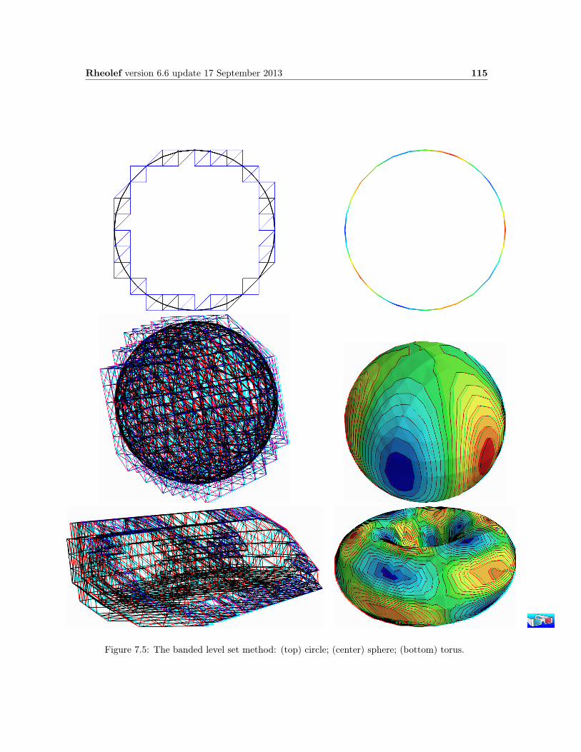
Rheolef version 6.6 update 17 September 2013 115
Figure 7.5: The banded level set method: (top) circle; (center) sphere; (bottom) torus.

116 Rheolef version 6.6 update 17 September 2013
cc0cc1cc2cc3cc4cc5cc6cc7cc8cc9
isolatedzero
Figure 7.6: The banded level set method: the band is composed of several connected components.

Chapter 8
The highly nonlinear p-laplacianproblem
8.1 Problem statement
Let us consider the classical p-Laplacian problem with homogeneous Dirichlet boundary conditionsin a domain bounded Ω ⊂ Rd, d = 1, 2, 3:(P): find u, defined in Ω such that:
−div(η(|∇u|2
)∇u)
= f in Ω
u = 0 on ∂Ω
where η : z ∈ R+ 7−→ zp−2
2 ∈ R+. Several variants of the η can be considered: see [44] for practicaland usefull examples. Here p ∈]1,+∞[ and f are known. For the computational examples, wechoose f = 1. When p = 2, this problem reduces to the linear Poisson problem with homogeneousDirichlet boundary conditions. Otherwise, for any p > 1, the nonlinear problem is equivalent tothe following minimization problem:(MP): find u ∈W 1,p
0 (Ω) such that:
u = arg minv∈W 1,p
0 (Ω)
1
2
∫
Ω
H(|∇v|2
)dx−
∫
Ω
f v dx,
where H denotes the primitive of η:
H(z) =
∫ z
0
η(z) dz =2zp
p
Here W 1,p0 (Ω) denotes the usual Sobolev spaces of functions in W 1,p(Ω) We also assume that f ∈
W−1,p(Ω), where W−1,p0 (Ω) denotes the dual space of W 1,p
0 (Ω) that vanishes on the boundary [8,p. 118]. The variational formulation of this problem expresses:(VF): find u ∈W 1,p
0 (Ω) such that:
a(u;u, v) = l(v), ∀v ∈W 1,p0 (Ω)
where a(., .) and l(.) are defined for any u0, u, v ∈W 1,p(Ω) by
a(u0;u, v) =
∫
Ω
η(|∇u0|2
)∇u.∇v dx, ∀u, v ∈W 1,p
0 (Ω) (8.1)
l(v) =
∫
Ω
f v dx, ∀u, v ∈ L2(Ω) (8.2)
The quantity a(u;u, u)1/p = ‖∇u‖0,p,Ω induces a norm in W 1,p0 , equivalent to the standard norm.
The form a(.; ., .) is bilinear with respect to the two last variable and is related to the energy form.
117

118 Rheolef version 6.6 update 17 September 2013
8.2 The fixed-point algorithm
8.2.1 Principe of the algorithm
This nonlinear problem is then reduced to a sequence of linear subproblems by using the fixed-pointalgorithm. The sequence
(u(n)
)n>0
is defined by recurrence as:
• n = 0: let u(0) ∈W 1,p0 (Ω) be known.
• n > 0: suppose that u(n) ∈W 1,p0 (Ω) is known and find u∗ ∈W 1,p
0 (Ω) such that:
a(u(n);u∗, v
)= l(v), ∀v ∈W 1,p
0 (Ω)
and then set
u(n+1) = ωu∗ + (1− ω) ∗ u(n)
Here ω > 0 is the relaxation parameter: when ω = 1 we obtain the usual un-relaxed fixed pointalgorithm. For stiff nonlinear problems, we will consider the under-relaxed case 0 < ω < 1. Letu(n+1) = G
(u(n)
)denotes the operator that solve the previous linear subproblem for a given u(n).
Since the solution u satisfies u = G(u), it is a fixed-point of G.Let us introduce a mesh Th of Ω and the finite dimensional space Xh of continuous piecewise poly-nomial functions and Vh, the subspace of Xh containing elements that vanishes on the boundaryof Ω:
Xh = vh ∈ C00
(Ω)
; vh/K ∈ Pk, ∀K ∈ ThVh = vh ∈ Xh; vh = 0 on ∂Ω
where k = 1 or 2. The approximate problem expresses: suppose that u(n)h ∈ Vh is known and find
u∗h ∈ Vh such that:
a(u
(n)h ;u∗h, vh
)= l(vh), ∀vh ∈ Vh
By developing u∗h on a basis of Vh, this problem reduces to a linear system.
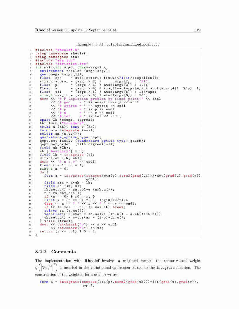
Rheolef version 6.6 update 17 September 2013 119
Example file 8.1: p_laplacian_fixed_point.cc1 #include "rheolef.h"2 using namespace rheolef;3 using namespace std;4 #include "eta.icc"5 #include "dirichlet.icc"6 int main(int argc , char**argv) 7 environment rheolef (argc ,argv);8 geo omega (argv [1]);9 Float eps = std:: numeric_limits <Float >:: epsilon ();
10 string approx = (argc > 2) ? argv [2] : "P1";11 Float p = (argc > 3) ? atof(argv [3]) : 1.5;12 Float w = (argc > 4) ? (is_float(argv [4]) ? atof(argv [4]) :2/p) :1;13 Float tol = (argc > 5) ? atof(argv [5]) : 1e5*eps;14 size_t max_it = (argc > 6) ? atoi(argv [6]) : 500;15 derr << "# P-Laplacian problem by fixed -point:" << endl16 << "# geo = " << omega.name() << endl17 << "# approx = " << approx << endl18 << "# p = " << p << endl19 << "# w = " << w << endl20 << "# tol = " << tol << endl;21 space Xh (omega , approx );22 Xh.block ("boundary");23 trial u (Xh); test v (Xh);24 form m = integrate (u*v);25 solver sm (m.uu());26 quadrature_option_type qopt;27 qopt.set_family (quadrature_option_type ::gauss );28 qopt.set_order (2*Xh.degree ()-1);29 field uh (Xh);30 uh ["boundary"] = 0;31 field lh = integrate (v);32 dirichlet (lh, uh);33 derr << "# n r v" << endl;34 Float r = 1, r0 = 1;35 size_t n = 0;36 do 37 form a = integrate(compose(eta(p),norm2(grad(uh)))* dot(grad(u),grad(v)),38 qopt);39 field mrh = a*uh - lh;40 field rh (Xh, 0);41 rh.set_u () = sm.solve (mrh.u());42 r = rh.max_abs ();43 if (n == 0) r0 = r; 44 Float v = (n == 0) ? 0 : log10(r0/r)/n;45 derr << n << " " << r << " " << v << endl;46 if (r <= tol || n++ >= max_it) break;47 solver sa (a.uu());48 vec <Float > u_star = sa.solve (lh.u() - a.ub()*uh.b());49 uh.set_u () = w*u_star + (1-w)*uh.u();50 while (true);51 dout << catchmark("p") << p << endl52 << catchmark("u") << uh;53 return (r <= tol) ? 0 : 1;54
8.2.2 Comments
The implementation with Rheolef involves a weighted forms: the tensor-valued weight
η
(∣∣∣∇u(n)h
∣∣∣2)
is inserted in the variationnal expression passed to the integrate function. The
construction of the weighted form a(.; ., .) writes:
form a = integrate(compose(eta(p),norm2(grad(uh)))* dot(grad(u),grad(v)),qopt);
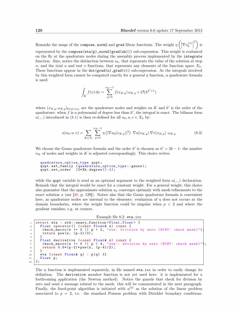
120 Rheolef version 6.6 update 17 September 2013
Remarks the usage of the compose, norm2 and grad libray functions. The weight η(∣∣∣∇u(n)
h
∣∣∣2)
is
represented by the compose(eta(p),norm2(grad(uh))) sub-expression. This weight is evaluatedon the fly at the quadrature nodes during the assembly process implemented by the integratefunction. Also, notice the distinction between uh, that represents the value of the solution at stepn, and the trial u and test v functions, that represents any elements of the function space Xh.These functions appear in the dot(grad(u),grad(v)) sub-expression. As the integrals involvedby this weighted form cannot be computed exactly for a general η function, a quadrature formulais used:
∫
K
f(x) dx =
nK−1∑
q=0
f(xK,q)ωK,q +O(hk′+1)
where (xK,q, ωK,q)06q<nKare the quadrature nodes and weights on K and k′ is the order of the
quadrature: when f is a polynomial of degree less than k′, the integral is exact. The bilinear forma(., .) introduced in (8.1) is then re-defined for all u0, u, v ∈ Xh by:
a(u0;u, v) =∑
K∈Th
nK−1∑
q=0
η(|∇u0(xK,q)|2
)∇u(xK,q).∇v(xK,q) ωK,q (8.3)
We choose the Gauss quadrature formula and the order k′ is choosen as k′ = 2k − 1: the numbernK of nodes and weights in K is adjusted correspondingly. This choice writes:
quadrature_option_type qopt;qopt.set_family (quadrature_option_type ::gauss );qopt.set_order (2*Xh.degree ()-1);
while the qopt variable is send as an optional argument to the weighted form a(., .) declaration.Remark that the integral would be exact for a constant weight. For a general weight, this choicealso guarantee that the approximate solution uh converges optimaly with mesh refinements to theexact solution u (see [38, p. 129]). Notice also that the Gauss quadrature formula is convenienthere, as quadrature nodes are internal to the elements: evaluation of η does not occurs at thedomain boundaries, where the weight function could be singular when p < 2 and where thegradient vanishes, e.g. at corners.
Example file 8.2: eta.icc1 struct eta : std:: unary_function <Float ,Float > 2 Float operator () (const Float& z) const 3 check_macro(z != 0 || p > 2, "eta: division by zero (HINT: check mesh)");4 return pow(z, (p -2)/2);5 6 Float derivative (const Float& z) const 7 check_macro(z != 0 || p > 4, "eta ’: division by zero (HINT: check mesh)");8 return 0.5*(p-2)* pow(z, (p -4)/2);9
10 eta (const Float& q) : p(q) 11 Float p;12 ;
The η function is implemented separately, in file named eta.icc in order to easily change itsdefinition. The derivative member function is not yet used here: it is implemented for aforthcoming application (the Newton method). Notice the guards that check for division byzero and send a message related to the mesh: this will be commentated in the next paragraph.Finally, the fixed-point algorithm is initiated with u(0) as the solution of the linear problemassociated to p = 2, i.e. the standard Poisson problem with Dirichlet boundary conditions.
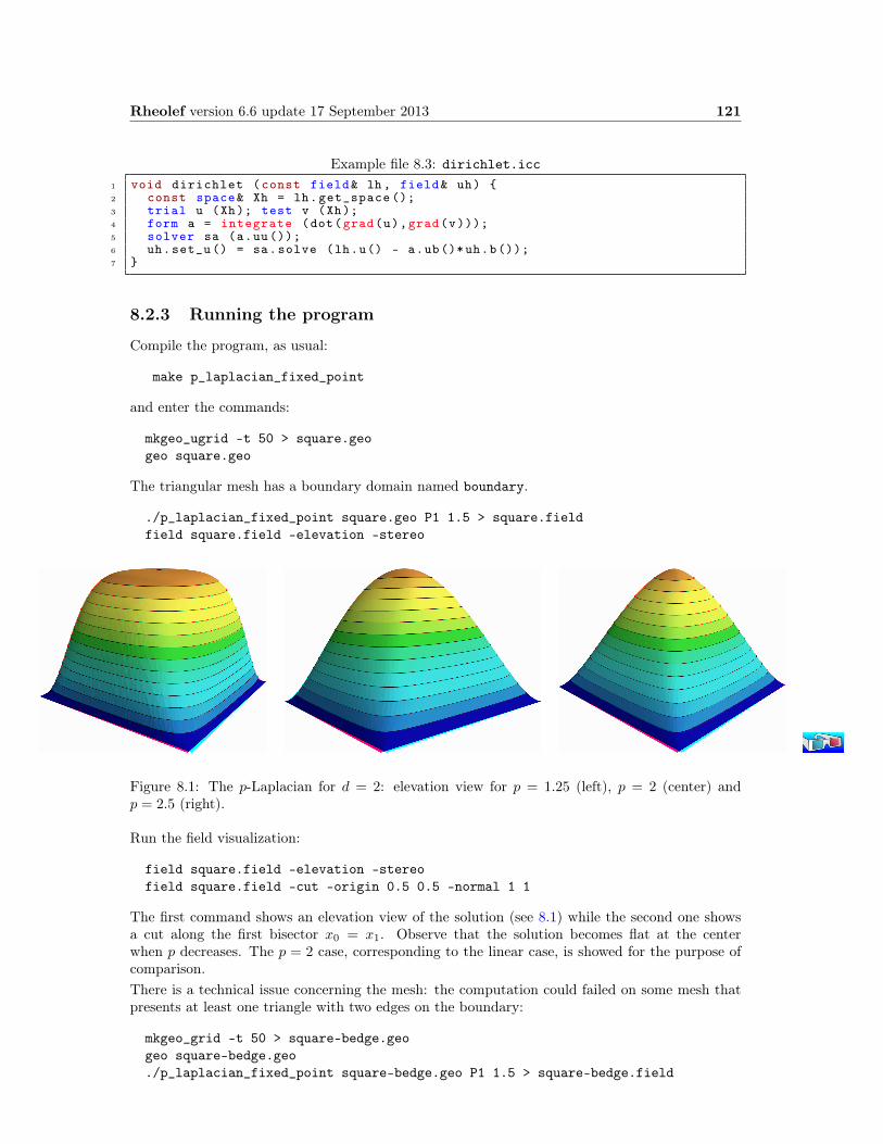
Rheolef version 6.6 update 17 September 2013 121
Example file 8.3: dirichlet.icc1 void dirichlet (const field& lh , field& uh) 2 const space& Xh = lh.get_space ();3 trial u (Xh); test v (Xh);4 form a = integrate (dot(grad(u),grad(v)));5 solver sa (a.uu());6 uh.set_u () = sa.solve (lh.u() - a.ub()*uh.b());7
8.2.3 Running the program
Compile the program, as usual:
make p_laplacian_fixed_point
and enter the commands:
mkgeo_ugrid -t 50 > square.geogeo square.geo
The triangular mesh has a boundary domain named boundary.
./p_laplacian_fixed_point square.geo P1 1.5 > square.fieldfield square.field -elevation -stereo
Figure 8.1: The p-Laplacian for d = 2: elevation view for p = 1.25 (left), p = 2 (center) andp = 2.5 (right).
Run the field visualization:
field square.field -elevation -stereofield square.field -cut -origin 0.5 0.5 -normal 1 1
The first command shows an elevation view of the solution (see 8.1) while the second one showsa cut along the first bisector x0 = x1. Observe that the solution becomes flat at the centerwhen p decreases. The p = 2 case, corresponding to the linear case, is showed for the purpose ofcomparison.There is a technical issue concerning the mesh: the computation could failed on some mesh thatpresents at least one triangle with two edges on the boundary:
mkgeo_grid -t 50 > square-bedge.geogeo square-bedge.geo./p_laplacian_fixed_point square-bedge.geo P1 1.5 > square-bedge.field
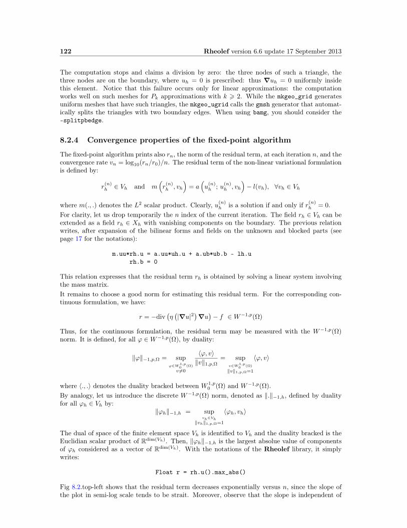
122 Rheolef version 6.6 update 17 September 2013
The computation stops and claims a division by zero: the three nodes of such a triangle, thethree nodes are on the boundary, where uh = 0 is prescribed: thus ∇uh = 0 uniformly insidethis element. Notice that this failure occurs only for linear approximations: the computationworks well on such meshes for Pk approximations with k > 2. While the mkgeo_grid generatesuniform meshes that have such triangles, the mkgeo_ugrid calls the gmsh generator that automat-ically splits the triangles with two boundary edges. When using bamg, you should consider the-splitpbedge.
8.2.4 Convergence properties of the fixed-point algorithm
The fixed-point algorithm prints also rn, the norm of the residual term, at each iteration n, and theconvergence rate vn = log10(rn/r0)/n. The residual term of the non-linear variational formulationis defined by:
r(n)h ∈ Vh and m
(r
(n)h , vh
)= a
(u
(n)h ; u
(n)h , vh
)− l(vh), ∀vh ∈ Vh
where m(., .) denotes the L2 scalar product. Clearly, u(n)h is a solution if and only if r(n)
h = 0.For clarity, let us drop temporarily the n index of the current iteration. The field rh ∈ Vh can beextended as a field rh ∈ Xh with vanishing components on the boundary. The previous relationwrites, after expansion of the bilinear forms and fields on the unknown and blocked parts (seepage 17 for the notations):
m.uu*rh.u = a.uu*uh.u + a.ub*ub.b - lh.urh.b = 0
This relation expresses that the residual term rh is obtained by solving a linear system involvingthe mass matrix.It remains to choose a good norm for estimating this residual term. For the corresponding con-tinuous formulation, we have:
r = −div(η(|∇u|2
)∇u)− f ∈W−1,p(Ω)
Thus, for the continuous formulation, the residual term may be measured with the W−1,p(Ω)norm. It is defined, for all ϕ ∈W−1,p(Ω), by duality:
‖ϕ‖−1,p,Ω = supϕ∈W1,p
0 (Ω)
v 6=0
〈ϕ, v〉‖v‖1,p,Ω
= supv∈W1,p
0 (Ω)
‖v‖1,p,Ω=1
〈ϕ, v〉
where 〈., .〉 denotes the duality bracked between W 1,p0 (Ω) and W−1,p(Ω).
By analogy, let us introduce the discrete W−1,p(Ω) norm, denoted as ‖.‖−1,h, defined by dualityfor all ϕh ∈ Vh by:
‖ϕh‖−1,h = supvh∈Vh
‖vh‖1,p,Ω=1
〈ϕh, vh〉
The dual of space of the finite element space Vh is identified to Vh and the duality bracked is theEuclidian scalar product of Rdim(Vh). Then, ‖ϕh‖−1,h is the largest absolue value of componentsof ϕh considered as a vector of Rdim(Vh). With the notations of the Rheolef library, it simplywrites:
Float r = rh.u().max_abs()
Fig 8.2.top-left shows that the residual term decreases exponentially versus n, since the slope ofthe plot in semi-log scale tends to be strait. Moreover, observe that the slope is independent of

Rheolef version 6.6 update 17 September 2013 123
10−15
10−10
10−5
1
0 25 50n
∥∥∥r(n)h
∥∥∥−1,h
p = 3/2
h = 1/10h = 1/20h = 1/30h = 1/40h = 1/50
10−15
10−10
10−5
1
0 25 50n
∥∥∥r(n)h
∥∥∥−1,h
p = 3/2
k = 1k = 2k = 3k = 4k = 5
10−15
10−10
10−5
1
0 250 500n
∥∥∥r(n)h
∥∥∥−1,h
p = 2.95p = 2.90p = 2.50
10−15
10−10
10−5
1
0 100 200n
∥∥∥r(n)h
∥∥∥−1,h
p = 1.15p = 1.25p = 1.50
Figure 8.2: The fixed-point algorithm on the p-Laplacian for d = 2: when p = 3/2, independenceof the convergence properties of the residue (top-left) with mesh refinement; (top-right) withpolynomial order Pk; when h = 1/50 and k = 1, convergence (bottom-left) for p > 2 and (bottom-right) for p < 2.
the mesh size h. Also, by vertue of the previous carreful definition of the residual term and itscorresponding norm, all the slopes falls into a master curve.These invariance properties applies also to the polynomial approximation Pk : Fig 8.2.top-rightshows that all the curves tends to collapse when k increases. Thus, the convergence propertiesof the algorithm are now investigated on a fixed mesh h = 1/50 and for a fixed polynomialapproximation k = 1.Fig 8.2.bottom-left and 8.2.bottom-right show the convergence vesus the power-law index p: ob-serve that the convergence becomes easier when p approaches p = 2, where the problem is linear.In that case, the convergence occurs in one iteration. Nevertheless, it appears two limitations.From one hand, when p → 3 the convergence starts to slow down and p > 3 cannot be solvedby this algorithm (it will be solved later in this chapter). From other hand, when p → 1, theconvergence slows down too and numerical rounding effets limits the convergence: the machineprecision canot be reached. Let us introduce the convergence rate vn = log10(rn/r0)/n it tends toa constant, denoted as v and: rn ≈ r0 × 10−v n. Observe on Fig 8.3.left that v tends to +∞ whenp = 2, since the system becomes linear and the algorithm converge in one iteration. Observe alsothat v tends to zero for p = 1 and p = 3 since the algorithm diverges. Fig 8.3.right shows thesame plot in semi-log scale and shows that v behaves as: v ≈ − log10 |p− 2|. This study shows
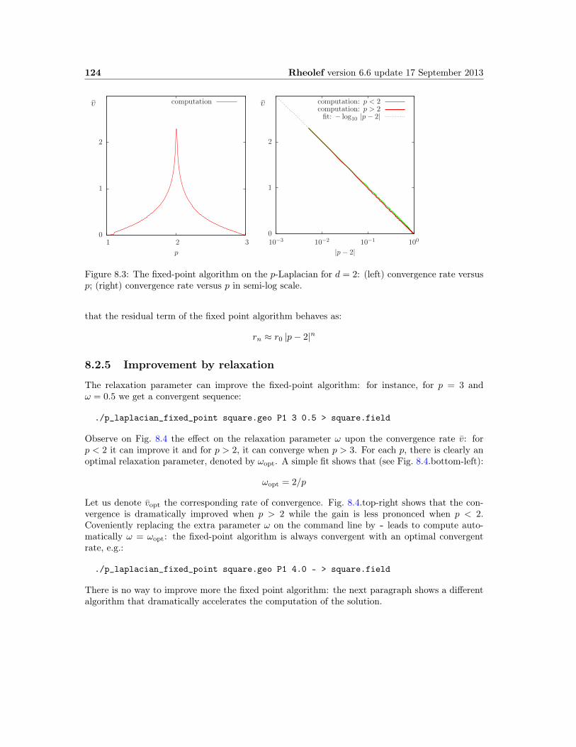
124 Rheolef version 6.6 update 17 September 2013
0
1
2
1 2 3p
v computation
0
1
2
10−3 10−2 10−1 100
|p − 2|
v computation: p < 2computation: p > 2
fit: − log10 |p− 2|
Figure 8.3: The fixed-point algorithm on the p-Laplacian for d = 2: (left) convergence rate versusp; (right) convergence rate versus p in semi-log scale.
that the residual term of the fixed point algorithm behaves as:
rn ≈ r0 |p− 2|n
8.2.5 Improvement by relaxation
The relaxation parameter can improve the fixed-point algorithm: for instance, for p = 3 andω = 0.5 we get a convergent sequence:
./p_laplacian_fixed_point square.geo P1 3 0.5 > square.field
Observe on Fig. 8.4 the effect on the relaxation parameter ω upon the convergence rate v: forp < 2 it can improve it and for p > 2, it can converge when p > 3. For each p, there is clearly anoptimal relaxation parameter, denoted by ωopt. A simple fit shows that (see Fig. 8.4.bottom-left):
ωopt = 2/p
Let us denote vopt the corresponding rate of convergence. Fig. 8.4.top-right shows that the con-vergence is dramatically improved when p > 2 while the gain is less prononced when p < 2.Coveniently replacing the extra parameter ω on the command line by - leads to compute auto-matically ω = ωopt: the fixed-point algorithm is always convergent with an optimal convergentrate, e.g.:
./p_laplacian_fixed_point square.geo P1 4.0 - > square.field
There is no way to improve more the fixed point algorithm: the next paragraph shows a differentalgorithm that dramatically accelerates the computation of the solution.

Rheolef version 6.6 update 17 September 2013 125
0
0.1
0.2
0.3
0.4
0 0.5 1 1.5 2ω
v p = 1.2p = 1.3p = 1.4p = 1.5
0
0.1
0.2
0.3
0.4
0 0.25 0.5 0.75 1ω
v p = 3p = 4p = 5p = 6
0
0.5
1
1.5
2
1 2 3 4 5 6 7 8p
ωoptcomputation: ωoptfit: ωopt(p) = 2/p
0
0.5
1
1.5
2
2.5
1 2 3 4 5 6 7 8p
vopt v when ω = ωopt
v when ω = 1
Figure 8.4: The fixed-point algorithm on the p-Laplacian for d = 2: effect of the relaxationparameter ω (top-left) when p < 2; (top-right) when p > 2; (bottom-left) optimal ωopt; (bottom-right) optimal vopt.
126 Rheolef version 6.6 update 17 September 2013
8.3 The Newton algorithm
8.3.1 Principe of the algorithm
An alternative to the fixed-point algorithm is to solve the nonlinear problem (P ) by using theNewton algorithm. Let us consider the following operator:
F : W 1,p0 (Ω) −→ W−1,p(Ω)u 7−→ F (u) = −div
(η(|∇u|2
)∇u)− f
The F operator computes simply the residual term and the problem expresses now as: find u ∈W 1,p
0 (Ω) such that F (u) = 0.The Newton algorithm reduces the nonlinear problem into a sequence of linear subproblems: thesequence
(u(n)
)n>0
is classically defined by recurrence as:
• n = 0: let u(0) ∈W 1,p0 (Ω) be known.
• n > 0: suppose that u(n) is known, find δu(n), defined in Ω, such that:
F ′(u(n)
)δu(n) = −F
(u(n)
)
and then compute explicitly:u(n+1) := u(n) + δu(n)
The notation F ′(u) stands for the Fréchet derivative of F , as an operator from W−1,p(Ω) intoW 1,p
0 (Ω). For any r ∈W−1,p(Ω), the linear tangent problem writes:find δu ∈W 1,p
0 (Ω) such that:
F ′(u) δu = −rAfter the computation of the Fréchet derivative, we obtain the strong form of this problem:(LT ): find δu, defined in Ω, such that
−div(η(|∇u|2
)∇(δu) + 2η′
(|∇u|2
)∇u.∇(δu)∇u
)= −r in Ω
δu = 0 on ∂Ω
whereη′(z) =
1
2(p− 2)z
p−42 , ∀z > 0
This is a Poisson-like problem with homogeneous Dirichlet boundary conditions and a non-constanttensorial coefficient. The variational form of the linear tangent problem writes:(V LT ): find δu ∈W 1,p
0 (Ω) such that
a1(u; δu, δv) = l1(v), ∀δv ∈W 1,p0 (Ω)
where the a1(.; ., .) is defined for any u, δu, δv ∈W 1,p0 (Ω) by:
a1(u; δu, δv) =
∫
Ω
(η(|∇u|2
)∇(δu).∇(δv) + 2η′
(|∇u|2
)∇u.∇(δu) ∇u.∇(δv)
)dx
l1(v) = −∫
Ω
r v dx
For any ξ ∈ Rd let us denote by ν(ξ) the following d× d matrix:
ν(ξ) = η(|ξ|2)I + 2η′
(|ξ|2)ξ ⊗ ξ

Rheolef version 6.6 update 17 September 2013 127
where I stands for the d-order identity matrix. Then the a1 expresses in a more compact form:
a1(u; δu, δv) =
∫
Ω
(ν(∇u)∇(δu)) .∇(δv) dx
Clearly a1 is linear and symmetric with respect to the two last variables.
Example file 8.4: p_laplacian_newton.cc1 #include "rheolef.h"2 using namespace rheolef;3 using namespace std;4 #include "p_laplacian.h"5 int main(int argc , char**argv) 6 environment rheolef (argc , argv);7 geo omega_h (argv [1]);8 Float eps = std:: numeric_limits <Float >:: epsilon ();9 string approx = (argc > 2) ? argv [2] : "P1";
10 Float p = (argc > 3) ? atof(argv [3]) : 1.5;11 Float tol = (argc > 4) ? atof(argv [4]) : 1e5*eps;12 size_t max_iter = (argc > 5) ? atoi(argv [5]) : 500;13 derr << "# P-Laplacian problem by Newton:" << endl14 << "# geo = " << omega_h.name() << endl15 << "# approx = " << approx << endl16 << "# p = " << p << endl17 << "# tol = " << tol << endl18 << "# max_iter = " << max_iter << endl;19 p_laplacian F (p, omega_h , approx );20 field uh = F.initial ();21 int status = newton (F, uh, tol , max_iter , &derr);22 dout << setprecision(numeric_limits <Float >:: digits10)23 << catchmark("p") << p << endl24 << catchmark("u") << uh;25 return status;26
Example file 8.5: p_laplacian.h1 class p_laplacian 2 public:3 typedef field value_type;4 typedef Float float_type;5 p_laplacian (Float p, const geo& omega , string approx );6 field initial () const;7 field residue (const field& uh) const;8 void update_derivative (const field& uh) const;9 field derivative_solve (const field& mrh) const;
10 field derivative_trans_mult (const field& mrh) const;11 Float space_norm (const field& uh) const;12 Float dual_space_norm (const field& mrh) const;13 Float duality_product (const field& mrh , const field& msh) const;14 Float p;15 space Xh;16 field lh;17 form m;18 solver sm;19 quadrature_option_type qopt;20 mutable form a1;21 mutable solver sa1;22 ;23 #include "p_laplacian1.icc"24 #include "p_laplacian2.icc"
8.3.2 Comments
The Newton algorithm is implemented in a generic way, for any F function, by the newton functionfrom the Rheolef librarys. The reference manual for the newton generic function is availableonline:
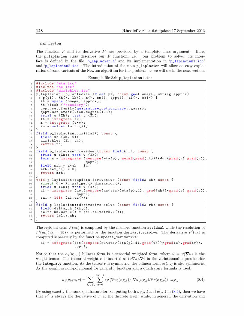
128 Rheolef version 6.6 update 17 September 2013
man newton
The function F and its derivative F ′ are provided by a template class argument. Here,the p_laplacian class describes our F function, i.e. our problem to solve: its inter-face is defined in the file ‘p_laplacian.h’ and its implementation in ‘p_laplacian1.icc’and ‘p_laplacian2.icc’. The introduction of the class p_laplacian will allow an easy explo-ration of some variants of the Newton algorithm for this problem, as we will see in the next section.
Example file 8.6: p_laplacian1.icc1 #include "eta.icc"2 #include "nu.icc"3 #include "dirichlet.icc"4 p_laplacian :: p_laplacian (Float p1, const geo& omega , string approx)5 : p(p1), Xh(), lh(), m(), sm(), qopt(), a1(), sa1() 6 Xh = space (omega , approx );7 Xh.block ("boundary");8 qopt.set_family(quadrature_option_type :: gauss );9 qopt.set_order (2*Xh.degree () -1);
10 trial u (Xh); test v (Xh);11 lh = integrate (v);12 m = integrate (u*v);13 sm = solver (m.uu());14 15 field p_laplacian :: initial () const 16 field uh (Xh, 0);17 dirichlet (lh, uh);18 return uh;19 20 field p_laplacian :: residue (const field& uh) const 21 trial u (Xh); test v (Xh);22 form a = integrate (compose(eta(p), norm2(grad(uh)))* dot(grad(u),grad(v)),23 qopt);24 field mrh = a*uh - lh;25 mrh.set_b () = 0;26 return mrh;27 28 void p_laplacian :: update_derivative (const field& uh) const 29 size_t d = Xh.get_geo (). dimension ();30 trial u (Xh); test v (Xh);31 a1 = integrate (dot(compose(nu <eta >(eta(p),d), grad(uh))* grad(u),grad(v)),32 qopt);33 sa1 = ldlt (a1.uu());34 35 field p_laplacian :: derivative_solve (const field& rh) const 36 field delta_uh (Xh ,0);37 delta_uh.set_u() = sa1.solve(rh.u());38 return delta_uh;39
The residual term F (uh) is computed by the member function residual while the resolution ofF ′(uh)δuh = Mrh is performed by the function derivative_solve. The derivative F ′(uh) iscomputed separately by the function update_derivative:
a1 = integrate(dot(compose(nu<eta >(eta(p),d),grad(uh))* grad(u),grad(v)),qopt);
Notice that the a1(u; ., .) bilinear form is a tensorial weighted form, where ν = ν(∇u) is theweight tensor. The tensorial weight ν is inserted as (ν∇u).∇v in the variationnal expression forthe integrate function. As the tensor ν is symmetric, the bilinear form a1(., .) is also symmetric.As the weight is non-polynomial for general η function and a quadrature formula is used:
a1(u0;u, v) =∑
K∈Th
nK−1∑
q=0
(ν (∇u0(xK,q)) ∇u(xK,q).∇v(xK,q)) ωK,q (8.4)
By using exactly the same quadrature for computing both a1(., .) and a(., .) in (8.4), then we havethat F ′ is always the derivative of F at the discrete level: while, in general, the derivation and
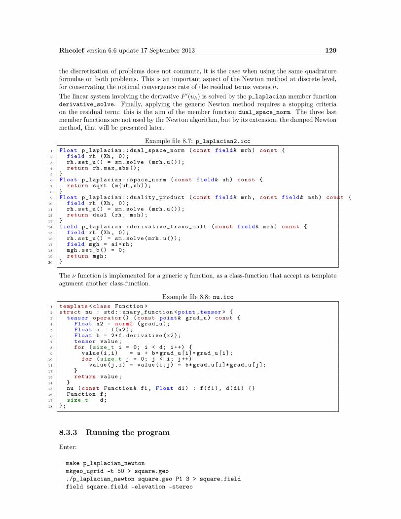
Rheolef version 6.6 update 17 September 2013 129
the discretization of problems does not commute, it is the case when using the same quadratureformulae on both problems. This is an important aspect of the Newton method at discrete level,for conservating the optimal convergence rate of the residual terms versus n.The linear system involving the derivative F ′(uh) is solved by the p_laplacian member functionderivative_solve. Finally, applying the generic Newton method requires a stopping criteriaon the residual term: this is the aim of the member function dual_space_norm. The three lastmember functions are not used by the Newton algorithm, but by its extension, the damped Newtonmethod, that will be presented later.
Example file 8.7: p_laplacian2.icc1 Float p_laplacian :: dual_space_norm (const field& mrh) const 2 field rh (Xh, 0);3 rh.set_u () = sm.solve (mrh.u());4 return rh.max_abs ();5 6 Float p_laplacian :: space_norm (const field& uh) const 7 return sqrt (m(uh,uh));8 9 Float p_laplacian :: duality_product (const field& mrh , const field& msh) const
10 field rh (Xh, 0);11 rh.set_u () = sm.solve (mrh.u());12 return dual (rh , msh);13 14 field p_laplacian :: derivative_trans_mult (const field& mrh) const 15 field rh (Xh, 0);16 rh.set_u () = sm.solve(mrh.u());17 field mgh = a1*rh;18 mgh.set_b () = 0;19 return mgh;20
The ν function is implemented for a generic η function, as a class-function that accept as templateagument another class-function.
Example file 8.8: nu.icc1 template <class Function >2 struct nu : std:: unary_function <point ,tensor > 3 tensor operator () (const point& grad_u) const 4 Float x2 = norm2 (grad_u );5 Float a = f(x2);6 Float b = 2*f.derivative(x2);7 tensor value;8 for (size_t i = 0; i < d; i++) 9 value(i,i) = a + b*grad_u[i]* grad_u[i];
10 for (size_t j = 0; j < i; j++)11 value(j,i) = value(i,j) = b*grad_u[i]* grad_u[j];12 13 return value;14 15 nu (const Function& f1, Float d1) : f(f1), d(d1) 16 Function f;17 size_t d;18 ;
8.3.3 Running the program
Enter:
make p_laplacian_newtonmkgeo_ugrid -t 50 > square.geo./p_laplacian_newton square.geo P1 3 > square.fieldfield square.field -elevation -stereo

130 Rheolef version 6.6 update 17 September 2013
10−15
10−10
10−5
1
0 5 10 15 20 25n
∥∥∥r(n)h
∥∥∥−1,h
p = 3
fixed point ω = 2/3Newton
Figure 8.5: The Newton algorithm on the p-laplacian for d = 2: comparison with the fixed-pointalgorithm.
The program prints at each iteration n, the residual term rn in discrete L2(Ω) norm. Convergenceoccurs in less than ten iterations: it dramatically improves the previous algorithm (see Fig. 8.5).Observe that the slope is no more constant in semi-log scale: the convergence rate accelerates andthe slope tends to be vertical, the so-called super-linear convergence. This is the major advantageof the Newton method. Figs. 8.6.top-left and. 8.6.top-bottom shows that the algorithm convergewhen p > 3 and that the convergence properties are independant of the mesh size h and thepolynomial order k. There are still two limitations of the method. From one hand, the Newtonalgorithm is no more independant of h and k when p 6 3/2 and to tends to diverges in thatcase when h tends to zero (see Fig. 8.6.bottom-left). From other hand, when p becomes large(see Fig. 8.6.bottom-right), an overshoot in the convergence tends to increases and distroys theconvergence, due to rounding problems. In order to circumvent these limitations, another strategyis considered in the next section: the damped Newton algorithm.

Rheolef version 6.6 update 17 September 2013 131
10−15
10−10
10−5
1
0 5 10 15 20 25n
∥∥∥r(n)h
∥∥∥−1,h
p = 3
h = 1/10h = 1/20h = 1/30h = 1/40h = 1/50
10−15
10−10
10−5
1
0 5 10 15 20 25n
∥∥∥r(n)h
∥∥∥−1,h
p = 3
k = 1k = 2k = 3k = 4k = 5
10−15
10−10
10−5
1
0 50 100n
∥∥∥r(n)h
∥∥∥−1,h
p = 3/2
h = 1/10h = 1/20h = 1/30h = 1/40h = 1/50
10−15
10−10
10−5
100
0 25n
∥∥∥r(n)h
∥∥∥−1,h
p = 2.5p = 3.0p = 3.5
Figure 8.6: The Newton algorithm on the p-laplacian for d = 2: (top-left) comparison with thefixed-point algorithm; when p = 3, independence of the convergence properties of the residue (top-left) with mesh refinement; (top-right) with polynomial order Pk; (bottom-left) mesh-dependenceconvergence when p < 2; (bottom-right) overshoot when p > 2.
132 Rheolef version 6.6 update 17 September 2013
8.4 The damped Newton algorithm
8.4.1 Principe of the algorithm
The Newton algorithm diverges when the initial u(0) is too far from a solution, e.g. when p isnot at the vicinity of 2. Our aim is to modify the Newton algorithm and to obtain a globallyconvergent algorithm, i.e to converge to a solution for any initial u(0). By this way, the algorithmshould converge for any value of p ∈]1,+∞[. The basic idea is to decrease the step length whilemaintaining the direction of the original Newton algorithm:
u(n+1) := u(n) + λn δu(n)
where λ(n) ∈]0, 1] and δu(n) is the direction from the Newton algorithm, given by:
F ′(u(n)
)δu(n) = −F
(u(n)
)
Let V a Banach space and let T : V → R defined for any v ∈ V by:
T (v) =1
2‖C−1F (v)‖2V ,
where C is some non-singular operator, easy to invert, used as a non-linear preconditioner. Thesimplest case, without preconditioner, is C = I. The T function furnishes a measure of the residualterm in L2 norm. The convergence is global when for any initial u(0), we have for any n > 0:
T(u(n+1)
)6 T
(u(n)
)+ α
⟨T ′(u(n)
), u(n+1) − u(n)
⟩V ′,V
(8.5)
where 〈., .〉V ′,V is the duality product between V and its dual V ′, and α ∈]0, 1[ is a small parameter.Notice that
T ′(u) = C−1F ′(u)∗C−1F (u)
where the superscript ∗ denotes the adjoint operator, i.e. the transpose matrix the in finitedimensional case. In practice we consider α = 10−4 and we also use a minimal step lengthλmin = 1/10 in order to avoid too small steps. Let us consider a fixed step n > 0: for conveniencethe n superscript is dropped in u(n) and δu(n). Let g : R→ R defined for any λ ∈ R by:
g(λ) = T (u+ λδu)
Then :
g′(λ) = 〈T ′(u+ λδu), δu〉V ′,V= 〈C−1F (u+ λδu), F ′(u+ λδu)C−1δu〉V,V ′
where the superscript ∗ denotes the adjoint operator, i.e. the transpose matrix the in finitedimensional case. The practical algorithm for obtaining λ was introduced first in [23] and is alsopresented in [37, p. 385]. The step length λ that satisfy (8.5) is computed by using a finite sequenceλk, k = 0, 1 . . . with a second order recurrence:
• k = 0 : initialization λ0 = 1. If (8.5) is satisfied with u + λ0 d then let λ := λ0 and thesequence stop here.
• k = 1 : first order recursion. The quantities g(0) = f(u) et g′(0) = 〈f ′(u), d〉 are alreadycomputed at initialization. Also, we already have computed g(1) = f(u+ d) when verifyingwhether (8.5) was satisfied. Thus, we consider the following approximation of g(λ) by asecond order polynomial:
g1(λ) = g(1)− g(0)− g′(0)λ2 + g′(0)λ+ g(0)

Rheolef version 6.6 update 17 September 2013 133
After a short computation, we find that the minimum of this polynomial is:
λ1 =−g′(0)
2g(1)− g(0)− g′(0)
Since the initialization at k = 0 does not satisfy (8.5), it is possible to show that, when α issmall enough, we have λ1 6 1/2 and λ1 ≈ 1/2. Let λ1 := max(λmin, λ1). If (8.5) is satisfiedwith u+ λ1 d then let λ := λ1 and the sequence stop here.
• k > 2 : second order recurrence. The quantities g(0) = f(u) et g′(0) =〉f ′(u), d〈 areavailable, together with λk−1, g(λk−1), λk−2 and g(λk−2). Then, g(λ) is approximated bythe following third order polynomial:
gk(λ) = aλ3 + bλ2 + g′(0)λ+ g(0)
where a et b are expressed by:
(ab
)=
1
λk−1 − λk−2
1
λ2k−1
− 1
λ2k−2
−λk−2
λ2k−1
λk−1
λ2k−2
(g(λk−1)− g′(0)λk−1 − g(0)g(λk−2)− g′(0)λk−2 − g(0)
)
The minimum of gk(λ) is
λk =−b+
√b2 − 3ag′(0)
3a
Let λk = min(1/2λk,max(λk/10, λk+1) in order for λk to be at the same order of magnitudeas λk−1. If (8.5) is satisfied with u+ λk d then let λ := λk and the sequence stop here.
The sequence (λk)k>0 is strictly decreasing: when the stopping criteria is not satisfied until λkreaches the machine precision εmach then the algorithm stops with an error.
Example file 8.9: p_laplacian_damped_newton.cc1 #include "rheolef.h"2 using namespace rheolef;3 using namespace std;4 #include "p_laplacian.h"5 int main(int argc , char**argv) 6 environment rheolef (argc ,argv);7 geo omega_h (argv [1]);8 Float eps = numeric_limits <Float >:: epsilon ();9 string approx = (argc > 2) ? argv [2] : "P1";
10 Float p = (argc > 3) ? atof(argv [3]) : 1.5;11 Float tol = (argc > 4) ? atof(argv [4]) : eps;12 size_t max_iter = (argc > 5) ? atoi(argv [5]) : 500;13 derr << "# P-Laplacian problem by damped Newton:" << endl14 << "# geo = " << omega_h.name() << endl15 << "# approx = " << approx << endl16 << "# p = " << p << endl;17 p_laplacian F (p, omega_h , approx );18 field uh = F.initial ();19 int status = damped_newton (F, uh , tol , max_iter , &derr);20 dout << catchmark("p") << p << endl21 << catchmark("u") << uh;22 return status;23
8.4.2 Comments
The damped_newton function implements the damped Newton algorithm for a generic T (u) func-tion, i.e. a generic nonlinear preconditioner. This algorithms use a backtrack strategy implemented
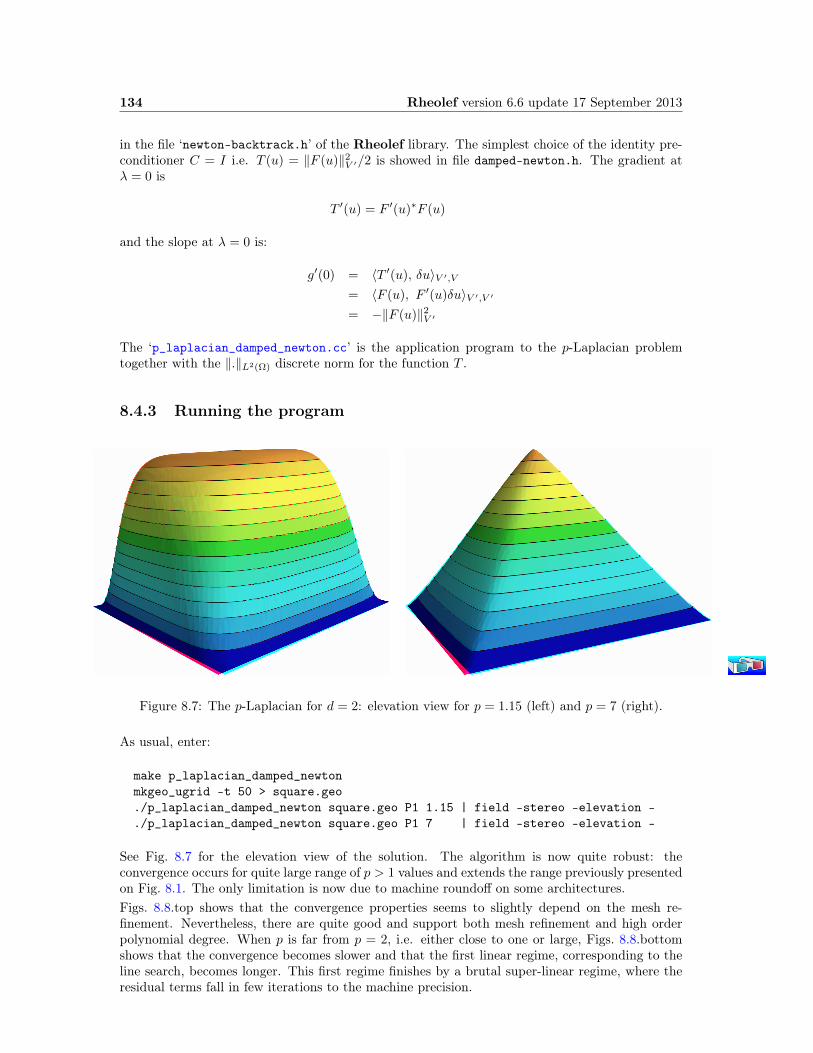
134 Rheolef version 6.6 update 17 September 2013
in the file ‘newton-backtrack.h’ of the Rheolef library. The simplest choice of the identity pre-conditioner C = I i.e. T (u) = ‖F (u)‖2V ′/2 is showed in file damped-newton.h. The gradient atλ = 0 is
T ′(u) = F ′(u)∗F (u)
and the slope at λ = 0 is:
g′(0) = 〈T ′(u), δu〉V ′,V= 〈F (u), F ′(u)δu〉V ′,V ′= −‖F (u)‖2V ′
The ‘p_laplacian_damped_newton.cc’ is the application program to the p-Laplacian problemtogether with the ‖.‖L2(Ω) discrete norm for the function T .
8.4.3 Running the program
Figure 8.7: The p-Laplacian for d = 2: elevation view for p = 1.15 (left) and p = 7 (right).
As usual, enter:
make p_laplacian_damped_newtonmkgeo_ugrid -t 50 > square.geo./p_laplacian_damped_newton square.geo P1 1.15 | field -stereo -elevation -./p_laplacian_damped_newton square.geo P1 7 | field -stereo -elevation -
See Fig. 8.7 for the elevation view of the solution. The algorithm is now quite robust: theconvergence occurs for quite large range of p > 1 values and extends the range previously presentedon Fig. 8.1. The only limitation is now due to machine roundoff on some architectures.Figs. 8.8.top shows that the convergence properties seems to slightly depend on the mesh re-finement. Nevertheless, there are quite good and support both mesh refinement and high orderpolynomial degree. When p is far from p = 2, i.e. either close to one or large, Figs. 8.8.bottomshows that the convergence becomes slower and that the first linear regime, corresponding to theline search, becomes longer. This first regime finishes by a brutal super-linear regime, where theresidual terms fall in few iterations to the machine precision.
Rheolef version 6.6 update 17 September 2013 135
8.5 Error analysis
While there is no simple explicit expression for the exact solution in the square Ω =]0, 1[2, thereis one when considering Ω as the unit circle:
u(x) =(p− 1) 2−
1p−1
p
(1−
(x2
0 + x21
) pp−1)
)
Example file 8.10: p_laplacian_circle.icc1 struct u_exact : field_functor <u_exact ,Float > 2 Float operator () (const point& x) const 3 return (1 - pow(norm2(x), p/(2*p -2)))/((p/(p -1))* pow (2. ,1/(p -1)));4 5 u_exact (Float q) : p(q) 6 protected: Float p;7 ;8 struct grad_u : field_functor <grad_u ,point > 9 point operator () (const point& x) const
10 return - (pow(norm2(x), p/(2*p-2) - 1)/pow (2. ,1/(p -1)))*x;11 12 grad_u (Float q) : p(q) 13 protected: Float p;14 ;
Example file 8.11: p_laplacian_error.cc1 #include "rheolef.h"2 using namespace rheolef;3 using namespace std;4 #include "p_laplacian_circle.icc"5 int main(int argc , char**argv) 6 environment rheolef (argc ,argv);7 Float tol = (argc > 1) ? atof(argv [1]) : 1e-15;8 Float p;9 field uh;
10 din >> catchmark("p") >> p11 >> catchmark("u") >> uh;12 const geo& omega = uh.get_geo ();13 const space& Xh = uh.get_space ();14 field pi_h_u = interpolate (Xh, u_exact(p));15 field eh = pi_h_u - uh;16 quadrature_option_type qopt;17 qopt.set_family(quadrature_option_type :: gauss );18 qopt.set_order (2*Xh.degree ());19 Float err_lp = pow(integrate (omega ,20 pow(fabs(uh - u_exact(p)), p), qopt), 1./p);21 Float err_w1p = pow(integrate (omega ,22 pow(norm(grad(uh) - grad_u(p)), p), qopt), 1./p);23 Float err_linf = eh.max_abs ();24 dout << "err_linf = " << err_linf << endl25 << "err_lp = " << err_lp << endl26 << "err_w1p = " << err_w1p << endl;27 return (err_linf < tol) ? 0 : 1;28
Notice, in the file ‘p_laplacian_error.cc’, the usage of the integrate function, together witha quadrature formula specificiation, for computing the errors in Lp norm and W 1,p semi-norm.Notice also the flexibility of expressions, mixing together fields as uh and field_functors, asu_exact. The whole expression is evaluated by the integrate function at quadrature pointsinside each element of the mesh.By this way, the error analysis investigation becomes easy:
make p_laplacian_errormkgeo_ball -t 10 -order 2 > circle-10-P2.geo./p_laplacian_damped_newton circle-10-P2.geo P2 1.5 | ./p_laplacian_error

136 Rheolef version 6.6 update 17 September 2013
We can vary both the mesh size and the polynomial order and the error plots are showed onFig. 8.9 for both the L2, L∞ norms and the W 1,p semi-norm. Observe the optimal error behavior:the slopes in the log-log scale are the same as those obtained by a direct Lagrange interpolationof the exact solution.

Rheolef version 6.6 update 17 September 2013 137
10−15
10−10
10−5
1
0 5 10 15 20 25n
∥∥∥r(n)h
∥∥∥−1,h
p = 3/2, k = 1
h = 1/10h = 1/20h = 1/30h = 1/40h = 1/50
10−15
10−10
10−5
1
0 5 10 15 20 25n
∥∥∥r(n)h
∥∥∥−1,h
p = 3/2, k = 1
k = 1k = 2k = 3k = 4k = 5
10−15
10−10
10−5
100
0 25 50n
∥∥∥r(n)h
∥∥∥−1,h
h = 1/50, k = 1
p = 1.5p = 1.4p = 1.3p = 1.2
10−15
10−10
10−5
100
0 5 10 15 20 25n
∥∥∥r(n)h
∥∥∥−1,h
h = 1/50, k = 1
p = 3p = 4p = 5p = 6p = 7
Figure 8.8: The damped Newton algorithm on the p-Laplacian for d = 2: when p = 1.5 andh = 1/50, convergence properties of the residue (top-left) with mesh refinement; (top-right) withpolynomial order Pk; (bottom-left) convergence when p < 2; (bottom-right) when p > 2.
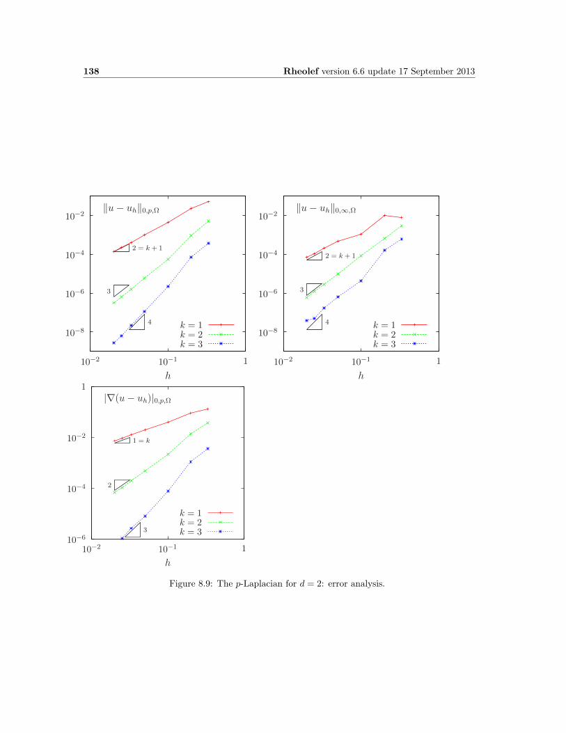
138 Rheolef version 6.6 update 17 September 2013
10−8
10−6
10−4
10−2
10−2 10−1 1
h
‖u− uh‖0,p,Ω
2 = k + 1
3
4 k = 1k = 2k = 3
10−8
10−6
10−4
10−2
10−2 10−1 1
h
‖u− uh‖0,∞,Ω
2 = k + 1
3
4 k = 1k = 2k = 3
10−6
10−4
10−2
1
10−2 10−1 1
h
|∇(u− uh)|0,p,Ω
1 = k
2
3
k = 1k = 2k = 3
Figure 8.9: The p-Laplacian for d = 2: error analysis.

Part IV
Technical appendices
139


Appendix A
How to write a variationalformulation ?
The major keypoint for using Rheolef is to put the problem in variational form. Then thisvariational form can be efficiently translated into C++ language. This appendix is dedicated toreaders who are not fluent with variational formulations and some related functionnal analysistools.
A.1 The Green formula
Let us come back to the model problem presented in section 1.1, page 15, equations (1.1)-(1.2)and details how this problem is transformed into (1.3).Let H1
0 (Ω) the space of functions whose gradient square has a finite sum over Ω and that vanisheson ∂Ω:
H10 (Ω) = v ∈ L2(Ω); ∇v ∈ L2(Ω)d and v = 0 on ∂Ω
We start by multiplying (1.1) by an arbitrarily test-function v ∈ H10 (Ω) and then integrate over Ω :
−∫
Ω
∆u v dx =
∫
Ω
f v dx, ∀v ∈ H10 (Ω)
The next step is to invoque an integration by part, the so-called Green formula:∫
Ω
∆u v dx+
∫
Ω
∇u.∇v dx =
∫
∂Ω
∂u
∂nv ds, ∀u, v ∈ H1(Ω)
Since our test-function v vanishes on the boundary, the integral over ∂Ω is zero and the problembecomes: ∫
Ω
∇u.∇v dx =
∫
Ω
f v dx, ∀v ∈ H10 (Ω)
This is exactly the variational formulation (1.3), page 15.
A.2 The vectorial Green formula
In this section, we come back to the linear elasticity problem presented in section 4.1, page 47,equations (4.1)-(4.2) and details how this problem is transformed into (4.3).Let Γd (resp. Γn) denotes the parts of the boundary ∂Ω related to the homogeneous Dirichletboundary condition u = 0 (resp. the homogeneous Neumann boundary condition σ(u)n = 0).
141
142 Rheolef version 6.6 update 17 September 2013
We suppose that ∂Ω = Γd ∩ Γn. Let us introduce the following functional space:
V = v ∈ H1(Ω)d; v = 0 on Γd
Then, multiplying the first equation of (4.2) by an arbitrarily test-function v ∈ V and thenintegrate over Ω :
−∫
Ω
div(σ(u)).v dx =
∫
Ω
f .v dx, ∀v ∈ V
The next step is to invoque an integration by part:∫
Ω
div τ.v dx+
∫
Ω
τ : D(v) dx =
∫
∂Ω
τ : (v ⊗ n) ds, ∀τ ∈ L2(Ω)d×d, ∀v ∈ V
Recall that div τ denotes(∑d−1
j=0 ∂jτi,j
)06i<d
, i.e. the vector whose component are the diver-
gence of each row of τ . Also, σ : τ denote the double contracted product∑d−1i,j=0 σi,jτi,j for any
tensors σ and τ , and that u ⊗ v dotes the τi,j = ui vj tensor, vectors u and v. Remark thatτ : (u⊗ v) = (τ v).u =
∑d−1i,j=0 τi,j ui vj . Choosing τ = σ(u) in the previous equation leads to:
∫
Ω
σ(u) : D(v) dx =
∫
∂Ω
(σ(u)n).v ds+
∫
Ω
f .v dx, ∀v ∈ V
Since our test-function v vanishes on Γd and the solution satisfie the homogeneous Neumannboundary condition σ(u)n = 0 on Γn, the integral over ∂Ω is zero and the problem becomes:
∫
Ω
σ(u) : D(v) dx =
∫
Ω
f .v dx, ∀v ∈ V
From the definition of σ(u) in (4.1) page 47 we have:
σ(u) : D(v) = λ div(u) (I : D(v)) + 2µD(u) : D(v)
= λ div(u) div(v) + 2µD(u) : D(v)
and the previous relation becomes:∫
Ω
λdiv(u) div(v) dx+
∫
Ω
2µD(u) : D(v) dx =
∫
Ω
f .v dx, ∀v ∈ V
This is exactly the variational formulation (4.3), page 48.
A.3 The Green formula on a surface
Let Γ a closed and orientable surface of Rd, d = 2, 3 and n its unit normal. From [25], appendix Cwe have the following integration by part:
∫
Γ
divsv ξ ds+
∫
Γ
v.∇sξ ds =
∫
Γ
v.n ξ divn ds
for all ξ ∈ H1(Γ) and v ∈ H1(Γ)d. Notice that divn represent the surface curvature. Next, wechoose v = ∇sϕ, for any ϕ ∈ H2(Γ). Remaking that v.n = 0 and that divsv = ∆sϕ. Then:
∫
Γ
∆s ξ ds+
∫
Γ
∇sϕ.∇sξ ds = 0
This formula is the starting point for all variational formulations of problems defined on a surface(see chapter 7).
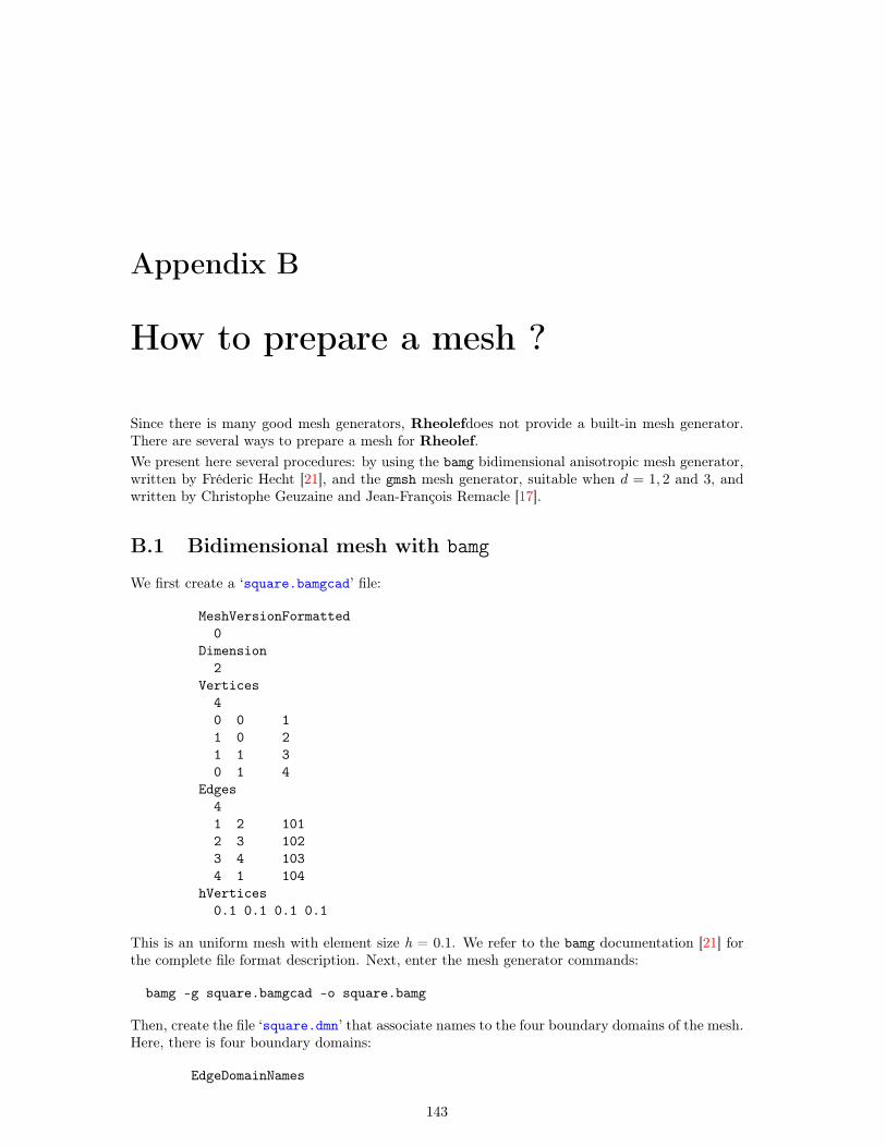
Appendix B
How to prepare a mesh ?
Since there is many good mesh generators, Rheolefdoes not provide a built-in mesh generator.There are several ways to prepare a mesh for Rheolef.We present here several procedures: by using the bamg bidimensional anisotropic mesh generator,written by Fréderic Hecht [21], and the gmsh mesh generator, suitable when d = 1, 2 and 3, andwritten by Christophe Geuzaine and Jean-François Remacle [17].
B.1 Bidimensional mesh with bamg
We first create a ‘square.bamgcad’ file:
MeshVersionFormatted0
Dimension2
Vertices40 0 11 0 21 1 30 1 4
Edges41 2 1012 3 1023 4 1034 1 104
hVertices0.1 0.1 0.1 0.1
This is an uniform mesh with element size h = 0.1. We refer to the bamg documentation [21] forthe complete file format description. Next, enter the mesh generator commands:
bamg -g square.bamgcad -o square.bamg
Then, create the file ‘square.dmn’ that associate names to the four boundary domains of the mesh.Here, there is four boundary domains:
EdgeDomainNames
143

144 Rheolef version 6.6 update 17 September 2013
4bottomrighttopleft
and enter the translation command:
bamg2geo square.bamg square.dmn > square.geo
This command creates a ‘square.geo’ file. Look at the mesh via the command:
geo square
This presents the mesh it in a graphical form, usually with gnuplot. You can switch to the mayavirenders:
geo square -mayavi
A finer mesh could be generated by:
bamg -coef 0.5 -g square.bamgcad -o square-0.5.bamg
B.2 Unidimensional mesh with gmsh
The simplest unidimensional mesh is a line:
h_local = 0.1;Point(1) = 0, 0, 0, h_local;Point(2) = 1, 0, 0, h_local;Line(3) = 1,2;Physical Point("left") = 1;Physical Point("right") = 2;Physical Point("boundary") = 1,2;Physical Line("interior") = 3;
The mesh generation command writes:
gmsh -1 line.mshcad -format msh -o line.msh
Then, the conversion to ‘.geo’ format and the visualization:
msh2geo line.msh > line.geogeo line
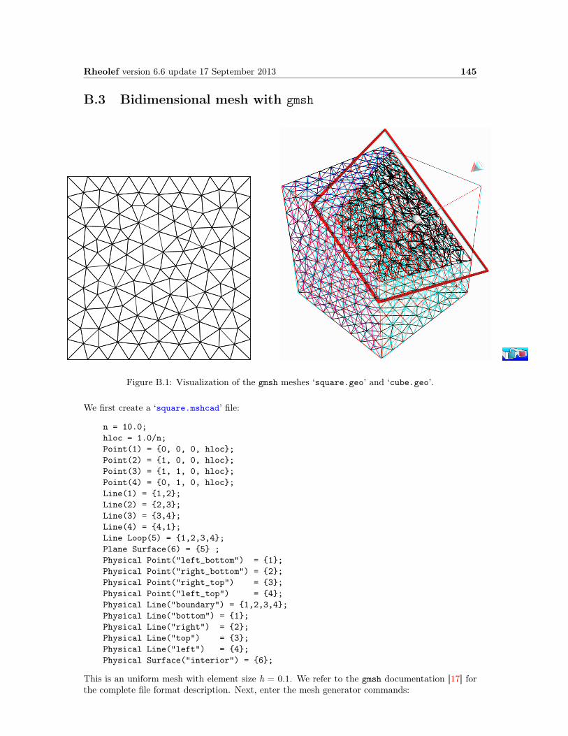
Rheolef version 6.6 update 17 September 2013 145
B.3 Bidimensional mesh with gmsh
Figure B.1: Visualization of the gmsh meshes ‘square.geo’ and ‘cube.geo’.
We first create a ‘square.mshcad’ file:
n = 10.0;hloc = 1.0/n;Point(1) = 0, 0, 0, hloc;Point(2) = 1, 0, 0, hloc;Point(3) = 1, 1, 0, hloc;Point(4) = 0, 1, 0, hloc;Line(1) = 1,2;Line(2) = 2,3;Line(3) = 3,4;Line(4) = 4,1;Line Loop(5) = 1,2,3,4;Plane Surface(6) = 5 ;Physical Point("left_bottom") = 1;Physical Point("right_bottom") = 2;Physical Point("right_top") = 3;Physical Point("left_top") = 4;Physical Line("boundary") = 1,2,3,4;Physical Line("bottom") = 1;Physical Line("right") = 2;Physical Line("top") = 3;Physical Line("left") = 4;Physical Surface("interior") = 6;
This is an uniform mesh with element size h = 0.1. We refer to the gmsh documentation [17] forthe complete file format description. Next, enter the mesh generator commands:
146 Rheolef version 6.6 update 17 September 2013
gmsh -2 square.mshcad -format msh -o square.msh
Then, enter the translation command:
msh2geo square.msh > square.geo
This command creates a ‘square.geo’ file. Look at the mesh via the command:
geo square
Remark that the domain names, defined in the .mshcad file, are included in the gmsh .msh inputfile and are propagated in the .geo by the format conversion.
B.4 Tridimensional mesh with gmsh
First, create a ‘cube.mshcad’ file:
Mesh.Algorithm = 7; // bamgMesh.Algorithm3D = 7; // mmg3da = 0; c = 0; f = 0;b = 1; d = 1; g = 1;n = 10;hloc = 1.0/n;Point(1) = a, c, f, hloc;Point(2) = b, c, f, hloc;Point(3) = b, d, f, hloc;Point(4) = a, d, f, hloc;Point(5) = a, c, g, hloc;Point(6) = b, c, g, hloc;Point(7) = b, d, g, hloc;Point(8) = a, d, g, hloc;Line(1) = 1,2;Line(2) = 2,3;Line(3) = 3,4;Line(4) = 4,1;Line(5) = 5,6;Line(6) = 6,7;Line(7) = 7,8;Line(8) = 8,5;Line(9) = 1,5;Line(10) = 2,6;Line(11) = 3,7;Line(12) = 4,8;Line Loop(21) = -1,-4,-3,-2;Plane Surface(31) = 21 ;Line Loop(22) = 5,6,7,8;Plane Surface(32) = 22 ;Line Loop(23) = 1,10,-5,-9;Plane Surface(33) = 23 ;Line Loop(24) = 12,-7,-11,3;Plane Surface(34) = 24 ;Line Loop(25) = 2,11,-6,-10;Plane Surface(35) = 25 ;Line Loop(26) = 9,-8,-12,4;

Rheolef version 6.6 update 17 September 2013 147
Plane Surface(36) = 26 ;Surface Loop(41) = 31,32,33,34,35,36;Volume(51) = 41;Physical Surface("bottom") = 31;Physical Surface("top") = 32;Physical Surface("left") = 33;Physical Surface("front") = 35;Physical Surface("right") = 34;Physical Surface("back") = 36;Physical Volume("internal") = 51;
Next, enter the mesh generator commands:
gmsh -3 cube.mshcad -format msh -o cube.msh
Then, enter the translation command:
msh2geo cube.msh > cube.geo
This command creates a ‘cube.geo’ file. Look at the mesh via the command:
geo cubegeo cube.geo -mayavi -cut
The second command allows to see inside the mesh.

148 Rheolef version 6.6 update 17 September 2013

Appendix C
Migrating to Rheolef version 6.0
Due to its new distributed memory and computation support, Rheolef version 6.0 presents somebackward incompatibilities with previous versions: codes using previous versions of the libraryshould be slightly modified. This appendix presents some indications for migrating existing code.
C.1 What is new in Rheolef 6.0 ?
The major main features are:
• support distributed achitectures: the code looks sequential, is easy to read and write butcan be run massively parallel and distributed, based on the MPI library.
• high order polynomial approximation: Pk basis are introduced in this version, for k > 0.This feature will be improved in the future developments.
• mesh adaptation and the charateristic method are now available for three-dimensional problems.
In order to evoluate in these directions, internal data structures inside the library are completelyrewritten in a different way, and thus this version is a completely new library.Conversely, the library and unix command interfaces was as less as possible modified.Nevertheless, the user will find some few backward incompatibilities: 5.93 based codes will notdirectly compile with the 6.0 library version. Let us review how to move a code from 5.93 to 6.0version.
C.2 What should I have to change in my 5.x code ?
1. Namespace
The namespace rheolef was already introduced in last 5.93 version. Recall that a code usuallystarts with:
#include "rheolef.h"using namespace rheolef;
2. Environment
The MPI library requires initialisation and the two command line arguments. This initialisationis performed via the boost::mpi class environment: The code entry point writes:
149

150 Rheolef version 6.6 update 17 September 2013
int main (int argc , char** argv) environment rheolef (argc ,argv);...
3. Fields and forms data accessors
The accesses to unknown and blocked data was of a field uh was direct, as uh.u and uh.b.This access is no more possible in a distributed environment, as non-local value requests may beoptimized and thus, read and write access may be controled thought accessors. These accessorsare named uh.u() and uh.b() for read access, and uh.set_u() and uh.set_b() for write access.Similarly, a form a has accessors as a.uu().A typical 5.93 code writes:
ssk <Float > sa = ldlt(a.uu);uh.u = sa.solve (lh.u - a.ub*uh.b);
and the corresponding 6.0 code is:solver sa (a.uu());uh.set_u () = sa.solve (lh.u() - a.ub()*uh.b());
This major change in the library interface induces the most important work when porting to the6.0 version.Notice also that the old ssk<Float> class has been supersetted by the solver class, that man-ages both direct and iterative solvers in a more effective way. For three-dimensional problems,the iterative solver is the default while direct solvers are used otherwise. In the same spirit, asolver_abtb has been introduced, for Stokes-like mixed problem. These features facilitate thedimension-independent coding style provided by the Rheolef library.
4. Distributed input and output streams
Input and output sequential standard streams cin, cout and cerr may now replaced by distributedRheolef streams din, dout and derr as:
din >> omega;dout << uh;
These new streams are available togeher with the idiststream and odiststream classes of theRheolef library.
5. File formats ‘.geo’ and ‘.field’ have changed
The ‘.geo’ and ‘.field’ file formats have changed. The ‘.mfield’ is now obsolete: it has beenmerged into the ‘.field’ format that supports now multi-component fields. Also, the corre-sponding mfield unix command is obsolete, as these features are integrated in the field unixcommand.At this early stage of the 6.0 version, it is not yet possible to read the old ‘.geo’ format, but thisbackward compatibility will be assured soon.
6. Space on a domain
A space defined on a domain "boundary" of a mesh omega was defined in the 5.93 version as:space Wh (omega["boundary"], omega , "P1");
It writes now:space Wh (omega["boundary"], "P1");
as the repetition of omega is no more required.
Rheolef version 6.6 update 17 September 2013 151
7. Nonlinear expressions involving fields
Non-linear operations, such as sqrt(uh) or 1/uh was directly supported in Rheolef-5.x.space Xh (omega , "P1");field uh (Xh, 2.);field vh = 1/uh;
Notice that non-linear operations as 1/uh do not returns in general picewise polynomials whileuh*uh is piecewise quadratic. In Rheolef-5.x, the returned value was implicitly the Lagrangeinterpolant of the nonlinear expression in space Xh. For more clarity, Rheolef-6.x requires anexplicit call to the interpolate function and the code should write:
field vh = interpolate (Xh, 1/uh);
Notice that when the expression is linear, there is no need to call interpolate.
C.3 New features in Rheolef 6.4
TheRheolef-6.x code is in active developments. While backward compatibility s maintained since6.0, some styles and idioms evoluates in order to increase the expressivity and the flexibility of theinterface library. Here is the summary of these evolutions.
1. Nonlinear expressions
Nonlinear expressions has been extended since Rheolef-6.4 to expression mixing field and func-tions or field_functor. For instance, when u_exact is a field_functor, an L2 error could becomputed using a nonlinear expression submitted to the integrate function:
Float err_l2 = sqrt (integrate (omega , sqr (uh - u_exact ()), qopt ));
2. Right-hand-side specification
For specifiying a right-hand-side involving f, previous code style, from Rheolef-6.0 to 6.3 wasusing:
field lh = riesz (Xh , f());
Rheolef-6.4 introduces:test v (Xh);field lh = integrate (f()*v);
This feature opens new possibilities of right-hand-side specifications, e.g. expressions involvingsome derivatives of the test-function v. The riesz function is no more needed: it is maintainedfor backward compatibility purpose.
3. Form specification
For specifiying a bilinear form, previous code style, from Rheolef-6.0 to 6.3 was using a specifi-cation based on a name:
form a (Xh , Xh , "grad_grad");
Rheolef-6.4 introduces:trial u (Xh); test v (Xh);form a = integrate (dot(grad(u),grad(v)));
This feature opens new possibilities for form specifications and more flexibility. The form specifi-cation based on a name is no more needed: it is maintained for backward compatibility purpose.

152 Rheolef version 6.6 update 17 September 2013
Appendix D
GNU Free Documentation License
Version 1.1, March 2000
Copyright c© 2000 Free Software Foundation, Inc.59 Temple Place, Suite 330, Boston, MA 02111-1307 USAEveryone is permitted to copy and distribute verbatim copies of this license document, but chang-ing it is not allowed.
*
PreambleThe purpose of this License is to make a manual, textbook, or other written document “free”in the sense of freedom: to assure everyone the effective freedom to copy and redistribute it,with or without modifying it, either commercially or noncommercially. Secondarily, this Licensepreserves for the author and publisher a way to get credit for their work, while not being consideredresponsible for modifications made by others.This License is a kind of “copyleft”, which means that derivative works of the document mustthemselves be free in the same sense. It complements the GNU General Public License, which isa copyleft license designed for free software.We have designed this License in order to use it for manuals for free software, because free softwareneeds free documentation: a free program should come with manuals providing the same freedomsthat the software does. But this License is not limited to software manuals; it can be used forany textual work, regardless of subject matter or whether it is published as a printed book. Werecommend this License principally for works whose purpose is instruction or reference.
Applicability and Definitions
This License applies to any manual or other work that contains a notice placed by the copyrightholder saying it can be distributed under the terms of this License. The “Document”, below, refersto any such manual or work. Any member of the public is a licensee, and is addressed as “you”.A “Modified Version” of the Document means any work containing the Document or a portion ofit, either copied verbatim, or with modifications and/or translated into another language.A “Secondary Section” is a named appendix or a front-matter section of the Document that dealsexclusively with the relationship of the publishers or authors of the Document to the Document’soverall subject (or to related matters) and contains nothing that could fall directly within thatoverall subject. (For example, if the Document is in part a textbook of mathematics, a Secondary
153
154 Rheolef version 6.6 update 17 September 2013
Section may not explain any mathematics.) The relationship could be a matter of historicalconnection with the subject or with related matters, or of legal, commercial, philosophical, ethicalor political position regarding them.The “Invariant Sections” are certain Secondary Sections whose titles are designated, as being thoseof Invariant Sections, in the notice that says that the Document is released under this License.The “Cover Texts” are certain short passages of text that are listed, as Front-Cover Texts orBack-Cover Texts, in the notice that says that the Document is released under this License.A “Transparent” copy of the Document means a machine-readable copy, represented in a formatwhose specification is available to the general public, whose contents can be viewed and editeddirectly and straightforwardly with generic text editors or (for images composed of pixels) genericpaint programs or (for drawings) some widely available drawing editor, and that is suitable forinput to text formatters or for automatic translation to a variety of formats suitable for input totext formatters. A copy made in an otherwise Transparent file format whose markup has beendesigned to thwart or discourage subsequent modification by readers is not Transparent. A copythat is not “Transparent” is called “Opaque”.Examples of suitable formats for Transparent copies include plain ASCII without markup, Texinfoinput format, LATEX input format, SGML or XML using a publicly available DTD, and standard-conforming simple HTML designed for human modification. Opaque formats include PostScript,PDF, proprietary formats that can be read and edited only by proprietary word processors, SGMLor XML for which the DTD and/or processing tools are not generally available, and the machine-generated HTML produced by some word processors for output purposes only.The “Title Page” means, for a printed book, the title page itself, plus such following pages as areneeded to hold, legibly, the material this License requires to appear in the title page. For worksin formats which do not have any title page as such, “Title Page” means the text near the mostprominent appearance of the work’s title, preceding the beginning of the body of the text.
Verbatim Copying
You may copy and distribute the Document in any medium, either commercially or noncommer-cially, provided that this License, the copyright notices, and the license notice saying this Licenseapplies to the Document are reproduced in all copies, and that you add no other conditions what-soever to those of this License. You may not use technical measures to obstruct or control thereading or further copying of the copies you make or distribute. However, you may accept com-pensation in exchange for copies. If you distribute a large enough number of copies you must alsofollow the conditions in section 3.You may also lend copies, under the same conditions stated above, and you may publicly displaycopies.
Copying in Quantity
If you publish printed copies of the Document numbering more than 100, and the Document’slicense notice requires Cover Texts, you must enclose the copies in covers that carry, clearly andlegibly, all these Cover Texts: Front-Cover Texts on the front cover, and Back-Cover Texts onthe back cover. Both covers must also clearly and legibly identify you as the publisher of thesecopies. The front cover must present the full title with all words of the title equally prominentand visible. You may add other material on the covers in addition. Copying with changes limitedto the covers, as long as they preserve the title of the Document and satisfy these conditions, canbe treated as verbatim copying in other respects.If the required texts for either cover are too voluminous to fit legibly, you should put the first oneslisted (as many as fit reasonably) on the actual cover, and continue the rest onto adjacent pages.
Rheolef version 6.6 update 17 September 2013 155
If you publish or distribute Opaque copies of the Document numbering more than 100, you musteither include a machine-readable Transparent copy along with each Opaque copy, or state inor with each Opaque copy a publicly-accessible computer-network location containing a completeTransparent copy of the Document, free of added material, which the general network-using publichas access to download anonymously at no charge using public-standard network protocols. If youuse the latter option, you must take reasonably prudent steps, when you begin distribution ofOpaque copies in quantity, to ensure that this Transparent copy will remain thus accessible at thestated location until at least one year after the last time you distribute an Opaque copy (directlyor through your agents or retailers) of that edition to the public.It is requested, but not required, that you contact the authors of the Document well beforeredistributing any large number of copies, to give them a chance to provide you with an updatedversion of the Document.
Modifications
You may copy and distribute a Modified Version of the Document under the conditions of sections2 and 3 above, provided that you release the Modified Version under precisely this License, withthe Modified Version filling the role of the Document, thus licensing distribution and modificationof the Modified Version to whoever possesses a copy of it. In addition, you must do these thingsin the Modified Version:
• Use in the Title Page (and on the covers, if any) a title distinct from that of the Document,and from those of previous versions (which should, if there were any, be listed in the Historysection of the Document). You may use the same title as a previous version if the originalpublisher of that version gives permission.
• List on the Title Page, as authors, one or more persons or entities responsible for authorshipof the modifications in the Modified Version, together with at least five of the principalauthors of the Document (all of its principal authors, if it has less than five).
• State on the Title page the name of the publisher of the Modified Version, as the publisher.
• Preserve all the copyright notices of the Document.
• Add an appropriate copyright notice for your modifications adjacent to the other copyrightnotices.
• Include, immediately after the copyright notices, a license notice giving the public permissionto use the Modified Version under the terms of this License, in the form shown in theAddendum below.
• Preserve in that license notice the full lists of Invariant Sections and required Cover Textsgiven in the Document’s license notice.
• Include an unaltered copy of this License.
• Preserve the section entitled “History”, and its title, and add to it an item stating at leastthe title, year, new authors, and publisher of the Modified Version as given on the TitlePage. If there is no section entitled “History” in the Document, create one stating the title,year, authors, and publisher of the Document as given on its Title Page, then add an itemdescribing the Modified Version as stated in the previous sentence.
• Preserve the network location, if any, given in the Document for public access to a Trans-parent copy of the Document, and likewise the network locations given in the Documentfor previous versions it was based on. These may be placed in the “History” section. Youmay omit a network location for a work that was published at least four years before theDocument itself, or if the original publisher of the version it refers to gives permission.
156 Rheolef version 6.6 update 17 September 2013
• In any section entitled “Acknowledgements” or “Dedications”, preserve the section’s title, andpreserve in the section all the substance and tone of each of the contributor acknowledgementsand/or dedications given therein.
• Preserve all the Invariant Sections of the Document, unaltered in their text and in theirtitles. Section numbers or the equivalent are not considered part of the section titles.
• Delete any section entitled “Endorsements”. Such a section may not be included in theModified Version.
• Do not retitle any existing section as “Endorsements” or to conflict in title with any InvariantSection.
If the Modified Version includes new front-matter sections or appendices that qualify as SecondarySections and contain no material copied from the Document, you may at your option designatesome or all of these sections as invariant. To do this, add their titles to the list of Invariant Sectionsin the Modified Version’s license notice. These titles must be distinct from any other section titles.You may add a section entitled “Endorsements”, provided it contains nothing but endorsementsof your Modified Version by various parties – for example, statements of peer review or that thetext has been approved by an organization as the authoritative definition of a standard.You may add a passage of up to five words as a Front-Cover Text, and a passage of up to 25 words asa Back-Cover Text, to the end of the list of Cover Texts in the Modified Version. Only one passageof Front-Cover Text and one of Back-Cover Text may be added by (or through arrangements madeby) any one entity. If the Document already includes a cover text for the same cover, previouslyadded by you or by arrangement made by the same entity you are acting on behalf of, you may notadd another; but you may replace the old one, on explicit permission from the previous publisherthat added the old one.The author(s) and publisher(s) of the Document do not by this License give permission to usetheir names for publicity for or to assert or imply endorsement of any Modified Version.
Combining Documents
You may combine the Document with other documents released under this License, under the termsdefined in section 4 above for modified versions, provided that you include in the combination allof the Invariant Sections of all of the original documents, unmodified, and list them all as InvariantSections of your combined work in its license notice.The combined work need only contain one copy of this License, and multiple identical InvariantSections may be replaced with a single copy. If there are multiple Invariant Sections with the samename but different contents, make the title of each such section unique by adding at the end ofit, in parentheses, the name of the original author or publisher of that section if known, or else aunique number. Make the same adjustment to the section titles in the list of Invariant Sections inthe license notice of the combined work.In the combination, you must combine any sections entitled “History” in the various originaldocuments, forming one section entitled “History”; likewise combine any sections entitled “Ac-knowledgements”, and any sections entitled “Dedications”. You must delete all sections entitled“Endorsements.”
Collections of Documents
You may make a collection consisting of the Document and other documents released under thisLicense, and replace the individual copies of this License in the various documents with a single
Rheolef version 6.6 update 17 September 2013 157
copy that is included in the collection, provided that you follow the rules of this License forverbatim copying of each of the documents in all other respects.You may extract a single document from such a collection, and distribute it individually underthis License, provided you insert a copy of this License into the extracted document, and followthis License in all other respects regarding verbatim copying of that document.
Aggregation With Independent Works
A compilation of the Document or its derivatives with other separate and independent documentsor works, in or on a volume of a storage or distribution medium, does not as a whole countas a Modified Version of the Document, provided no compilation copyright is claimed for thecompilation. Such a compilation is called an “aggregate”, and this License does not apply tothe other self-contained works thus compiled with the Document, on account of their being thuscompiled, if they are not themselves derivative works of the Document.If the Cover Text requirement of section 3 is applicable to these copies of the Document, then ifthe Document is less than one quarter of the entire aggregate, the Document’s Cover Texts maybe placed on covers that surround only the Document within the aggregate. Otherwise they mustappear on covers around the whole aggregate.
Translation
Translation is considered a kind of modification, so you may distribute translations of the Docu-ment under the terms of section 4. Replacing Invariant Sections with translations requires specialpermission from their copyright holders, but you may include translations of some or all InvariantSections in addition to the original versions of these Invariant Sections. You may include a trans-lation of this License provided that you also include the original English version of this License.In case of a disagreement between the translation and the original English version of this License,the original English version will prevail.
Termination
You may not copy, modify, sublicense, or distribute the Document except as expressly providedfor under this License. Any other attempt to copy, modify, sublicense or distribute the Documentis void, and will automatically terminate your rights under this License. However, parties whohave received copies, or rights, from you under this License will not have their licenses terminatedso long as such parties remain in full compliance.
Future Revisions of This License
The Free Software Foundation may publish new, revised versions of the GNU Free DocumentationLicense from time to time. Such new versions will be similar in spirit to the present version, butmay differ in detail to address new problems or concerns. See http://www.gnu.org/copyleft.Each version of the License is given a distinguishing version number. If the Document specifiesthat a particular numbered version of this License "or any later version" applies to it, you have theoption of following the terms and conditions either of that specified version or of any later versionthat has been published (not as a draft) by the Free Software Foundation. If the Document doesnot specify a version number of this License, you may choose any version ever published (not asa draft) by the Free Software Foundation.
158 Rheolef version 6.6 update 17 September 2013
*
ADDENDUM: How to use this License for your documentsTo use this License in a document you have written, include a copy of the License in the documentand put the following copyright and license notices just after the title page:
Copyright c© YEAR YOUR NAME. Permission is granted to copy, distribute and/ormodify this document under the terms of the GNU Free Documentation License, Ver-sion 1.1 or any later version published by the Free Software Foundation; with theInvariant Sections being LIST THEIR TITLES, with the Front-Cover Texts beingLIST, and with the Back-Cover Texts being LIST. A copy of the license is included inthe section entitled “GNU Free Documentation License”.
If you have no Invariant Sections, write “with no Invariant Sections” instead of saying whichones are invariant. If you have no Front-Cover Texts, write “no Front-Cover Texts” instead of“Front-Cover Texts being LIST”; likewise for Back-Cover Texts.If your document contains nontrivial examples of program code, we recommend releasing theseexamples in parallel under your choice of free software license, such as the GNU General PublicLicense, to permit their use in free software.
Bibliography
[1] E. M. Abdalass. Résolution performante du problème de Stokes par mini-éléments, maillagesauto-adaptatifs et méthodes multigrilles – applications. PhD thesis, Thèse de l’école centralede Lyon, 1987. 68
[2] L. Abouorm. Méthodes mathématiques pour les écoulements sur des surfaces. PhD thesis,M2R Université J. Fourier, Grenoble, 2010. 109, 110
[3] D. N. Arnold, F. Brezzi, and M. Fortin. A stable finite element for the Stokes equations.Calcolo, 21:337–344, 1984. 67
[4] F. Auteri, N. Parolini, and L. Quartapelle. Numerical investigation on the stability of singulardriven cavity flow. J. Comput. Phys., 183(1):1–25, 2002. 93
[5] G. K. Batchelor. An introduction to fluid dynamics. Cambridge university press, UK, sixthedition, 1967. 73
[6] H. Borouchaki, P. L. George, F. Hecht, P. Laug, B. Mohammadi, and E. Saltel. Mailleurbidimensionnel de Delaunay gouverné par une carte de métriques. Partie II: applications.Technical Report RR-2760, INRIA, 1995. 54
[7] K. Boukir, Y. Maday, B. Metivet, and E. Razafindrakoto. A high-order characteristic/finiteelement method for the incompressible Navier-Stokes equations. Int. J. Numer. Meth. Fluids,25:1421–1454, 1997. 86
[8] H. Brezis. Analyse fonctionnelle. Théorie et application. Masson, Paris, 1983. 117
[9] F. Brezzi and J. Pitkäranta. On the stabilization of finite element approximation of the Stokesequations. In Efficient solutions of elliptic systems, Kiel, Notes on numerical fluid mechanics,volume 10, pages 11–19, 1984. 69
[10] M. J. Castro-Diaz, F. Hecht, B. Mohammadi, and O. Pironneau. Anisotropic unstructuredmesh adaption for flow simulations. Int. J. Numer. Meth. Fluids, 25(4):475–491, 1997. 54
[11] K. Deckelnick, G. Dziuk, C.M. Elliott, and C.-J. Heine. An h-narrow band finite elementmethod for elliptic equations on implicit surfaces. IMA Journal of Numerical Analysis, toappear:0, 2009. 98
[12] M. Dicko. Méthodes mathématiques pour les écoulements sur des surfaces. PhD thesis, M2PUniversité J. Fourier, Grenoble, 2011. 109
[13] J. Donea and A. Huerta. Finite element methods for flow problems. Wiley, New-York, 2003.92
[14] E. Erturk, T. C. Corke, and C. Gökçol. Numerical solutions of 2-D steady incompressibledriven cavity flow at high Reynolds numbers. Int. J. Numer. Meth. Fluids, 48:747–774, 2005.93
159

160 Rheolef version 6.6 update 17 September 2013
[15] G. Fourestey and S. Piperno. A second-order time-accurate ALE Lagrange-Galerkin methodapplied to wind engineering and control of bridge profiles. Comput. Methods Appl. Mech.Engrg., 193:4117–4137, 2004. 86
[16] T. Gelhard, G. Lube, M. A. Olshanskii, and J. H. Starcke. Stabilized finite element schemeswith LBB-stable elements for incompressible flows. J. Comput. Appl. Math., 177:243–267,2005. 93
[17] C. Geuzaine and J.-F. Remacle. Gmsh: a three-dimensional finite element mesh generatorwith built-in pre- and post-processing facilities. Int. J. Numer. Meths Engrg., 79(11):1309–1331, 2009. 143, 145
[18] U. Ghia, K. N. Ghia, and C. T. Shin. High Re solutions for incompressible flow using theNavier-Stokes equations and a multigrid method. J. Comput. Phys., 48:387–411, 1982. 92
[19] V. Girault and P. A. Raviart. Finite element methods for the Navier-Stokes equations. Theoryand algorithms. Springer, 1986. 35, 60, 62
[20] M. M. Gupta and J. C. Kalita. A new paradigm for solving Navier-Stokes equations:streamfunction-velocity formulation. J. Comput. Phys., 207:52–68, 2005. 92
[21] F. Hecht. BAMG: bidimensional anisotropic mesh generator, 2006. http://www.ann.jussieu.fr/~hecht/ftp/bamg. 54, 143
[22] P. Hood and C. Taylor. A numerical solution of the Navier-Stokes equations using the finiteelement technique. Comp. and Fluids, 1:73–100, 1973. 58, 66, 87
[23] Jr. J. E. Dennis and R. B. Schnablel. Numerical methods for unconstraint optimization andnonlinear equations. Prentice Hall, Englewood Cliff, N. J., 1983. 132
[24] A. Klawonn. An optimal preconditioner for a class of saddle point problems with a penaltyterm. SIAM J. Sci. Comput, 19(2):540–552, 1998. 59, 66
[25] A. Laadhari, C. Misbah, and P. Saramito. On the equilibrium equation for a generalizedbiological membrane energy by using a shape optimization approach. Phys. D, 239:1568–1572, 2010. 142
[26] R. J. Labeur and G. N. Wells. A Galerkin interface stabilisation method for the advection-diffusion and incompressible Navier-Stokes equations. Comput. Meth. Appl. Mech. Engrg.,196(49–52):4985–5000, 2007. 92
[27] S. Melchior, V. Legat, P. Van Dooren, and A. J. Wathen. Analysis of preconditioned iterativesolvers for incompressible flow problems. Int. J. Numer. Meth. Fluids, 2011. 93
[28] P. D. Minev and C. R. Ethier. A characteristic/finite element algorithm for the 3-D Navier-Stokes equations using unstructured grids. Comput. Meth. in Appl. Mech. and Engrg., 178(1-2):39–50, 1998. 93
[29] D. R. Musser and A. Saini. C++ STL tutorial and reference guide. Addison Wesley, Reading,1996. 24
[30] D. R. Musser and A. Saini. STL tutorial and reference guide. Addison-Wesley, 1996. 82
[31] M. A. Olshanskii and A. Reusken. A finite element method for surface PDEs: matrix prop-erties. Numer. Math., 114:491–520, 2010. 110
[32] M. A. Olshanskii, A. Reusken, and J. Grande. A finite element method for elliptic equationson surfaces. SIAM J. Num. Anal., 47(5):3339–3358, 2009. 104, 109, 110
Rheolef version 6.6 update 17 September 2013 161
[33] M. L. Ould Salihi. Couplage de méthodes numériques en simulation directe d’écoulementsincompressibles. PhD thesis, Université J. Fourier, Grenoble, 1998. 93
[34] C. C. Paige and M. A. Saunders. Solution of sparse indefinite systems of linear equations.SIAM J. Numer. Anal., 12(4):617–629, 1975. 35
[35] O. Pironneau. Méthode des éléments finis pour les fluides. Masson, Paris, 1988. 81
[36] O. Pironneau and M. Tabata. Stability and convergence of a galerkin-characteristics finiteelement scheme of lumped mass type. Int. J. Numer. Meth. Fluids, 64:1240–1253, 2010. 82
[37] W. H. Press, S. A. Teulkolsky, W. T. Vetterling, and B. P. Flannery. Numerical recepies inC. The art of scientific computing. Cambridge University Press, UK, second edition, 1997.Version 2.08. 132
[38] P. A. Raviart and J. M. Thomas. Introduction à l’analyse numerique des équations auxdérivées partielles. Masson, Paris, 1983. 120
[39] N. Roquet, R. Michel, and P. Saramito. Errors estimate for a viscoplastic fluid by using Pkfinite elements and adaptive meshes. C. R. Acad. Sci. Paris, ser. I, 331(7):563–568, 2000. 54
[40] H. Rui and M. Tabata. A second order characteristic finite element scheme for convectiondiffusion problems. Numer. Math. (to appear), 2001. 81
[41] P. Saramito. Simulation numérique d’écoulements de fluides viscoélastiques par éléments finisincompressibles et une méthode de directions alternées; applications. PhD thesis, InstitutNational Polytechnique de Grenoble, 1990. 73
[42] P. Saramito. Rheolef home page. http://www-lmc.imag.fr/lmc-edp/Pierre.Saramito/rheolef, 2012. 25
[43] P. Saramito. Language C++ et calcul scientifique. CNRS-CCSD, 2012. http://cel.archives-ouvertes.fr/cel-00573975. 3
[44] P. Saramito. Méthodes numériques en fluides complexes : théorie et algorithmes. CNRS-CCSD, 2012. http://cel.archives-ouvertes.fr/cel-00673816. 117
[45] P. Saramito and N. Roquet. An adaptive finite element method for viscoplastic fluid flows inpipes. Comput. Meth. Applied Mech. Engng, 190(40-41):5391–5412, 2001. 22
[46] Pierre Saramito. Are curved and high order gmsh meshes really high order ?, 2012. http://www.geuz.org/pipermail/gmsh/2012/006967.html. 105
[47] J. Shen. Hopf bifurcation of the unsteady regularized driven cavity flow. J. Comp. Phys.,95:228–245, 1991. http://www.math.purdue.edu/~shen/pub/Cavity.pdf. 93
[48] B. Stroustrup. The C++ programming language. Addison Wesley, Reading, special edition,1997. 3
[49] B. Stroustrup. C++ programming styles and libraries. InformIt.com, 0:0, 2002. 2
[50] M.-G. Vallet. Génération de maillages anisotropes adaptés, application à la capture de coucheslimites. Technical Report RR-1360, INRIA, 1990. 54
[51] Wikipedia. The Stokes stream function. Wikipedia, 2012. http://en.wikipedia.org/wiki/Stokes_stream_function. 73
[52] N. Wirth. Algorithm + data structure = programs. Prentice Hall, NJ, USA, 1985. 2

List of example files
Makefile, 16cavity.icc, 56convect.cc, 79convect_error.cc, 81cosinusprod.icc, 24cosinusprod_error.cc, 24cosinusprod_laplace.icc, 22cosinusrad.icc, 26cosinusrad_laplace.icc, 26dirichlet-nh.cc, 22dirichlet.cc, 14dirichlet.icc, 119elasticity_criterion.icc, 53elasticity_solve.icc, 53embankment.cc, 47embankment.icc, 47embankment_adapt.cc, 52eta.icc, 118heat.cc, 75helmholtz_band.cc, 109helmholtz_band_iterative.cc, 107helmholtz_s.cc, 96incompressible-elasticity.cc, 64laplace_band.cc, 110laplace_s.cc, 101level_set_sphere.cc, 104navier_stokes_cavity.cc, 86navier_stokes_criterion.icc, 87navier_stokes_solve.icc, 85neumann-laplace.cc, 34neumann-nh.cc, 30nu.icc, 127p_laplacian.h, 125p_laplacian1.icc, 126p_laplacian2.icc, 127p_laplacian_circle.icc, 133p_laplacian_damped_newton.cc, 131p_laplacian_error.cc, 133p_laplacian_fixed_point.cc, 116p_laplacian_newton.cc, 125poiseuille.h, 68proj_band.cc, 108robin.cc, 32
rotating-hill.h, 80sinusprod_helmholtz.icc, 31sphere.icc, 97stokes_cavity.cc, 56stokes_contraction_bubble.cc, 67streamf_cavity.cc, 61streamf_contraction.cc, 70stress.cc, 49torus.icc, 101transmission.cc, 38vortex_position.cc, 91vorticity.cc, 59cavity.icc, 87contraction.mshcad, 68, 72convect.cc, 86cosinusrad_error.cc, 26cube.mshcad, 144dirichlet_nh_ball.cc, 26helmholtz_s_error.cc, 99line.mshcad, 55, 142neumann-nh.cc, 96square.bamgcad, 54, 89, 141square.dmn, 54, 89, 141square.mshcad, 143stokes_contraction.cc, 70streamf_cavity.cc, 89streamf_contraction.cc, 72stress.cc, 74torus.mshcad, 103
162
List of commands
bamg2geo, 141bamg, 54, 89, 141
-splitpbedge, 120branch, 80
-gnuplot, 78-paraview, 78, 83-umax, 78
convect, 80ffmpeg, 78field, 17, 148
-, 19-bw, 18, 70, 73, 89-catchmark, 58-comp, 49, 52, 73, 90-cut, 73, 90, 119-elevation, 18, 51, 108, 119-fill, 49-gray, 18-iso, 52-max, 71, 90-mayavi, 18, 49-min, 90-n-iso, 70-n-iso-negative, 70, 73, 89-noclean, 62-noexecute, 62-nofill, 18, 49-normal, 73, 90, 119-origin, 73, 90, 119-proj, 51-scale, 65, 89-stereo, 18, 20, 49, 51-velocity, 58, 89
geo, 17-cut, 19-full, 19-stereo, 19-subdivide, 98
gmsh, 55, 68, 72, 97, 103, 120, 142gnuplot, 17, 19, 40, 49, 78, 81, 142gzip, 54library
boost, 15, 35, 147CGAL, computational geometry, 79
MPI, message passing interface,15, 147
STL, standard template library, 80make, 16man, 19mayavi, 18, 20, 62, 142mkgeo_ball, 97
-e, 97-q, 26-s, 97-t, 26, 97
mkgeo_grid, 17, 80, 120-H, 20-T, 19, 83-a, 81-b, 81-c, 83-d, 83-e, 19-f, 83-g, 83-q, 20-region, 40-t, 17-zr, 71
mkgeo_ugrid, 26, 120mpirun, 17, 35, 41msh2geo, 68, 142, 144
-zr, 72paraview, 78, 83rheolef-config, 13
–check, 13–docdir, 13–exampledir, 13
sed, 26visualization
mesh, 17deformed, 49
vlc, 78zcat, 89
163
Index
approximation, 14P0, 51P1b-P1, 65P1d, 51P1, 15, 47, 51, 64, 65, 84P2-P1, Taylor-Hood, 56, 65, 66, 70P2, 15, 19, 47, 51, 64, 84Pk, 15, 19, 147bubble, 65discontinuous, 39, 50, 51, 59high-order, 15, 19, 41, 147isoparametric, 98mixed, 56
argc, argv, command line arguments, 15, 147
BDF2 scheme, 84benchmark
driven cavity flow, 55, 84Dziuk-Elliott-Heine on a sphere, 96embankment, 45flow in an abrupt contraction, 66, 72Olshanskii-Reusken-Grande on a torus,
102rotating hill, 79
boundary conditionDirichlet, 13, 21, 39, 45, 55, 63, 84, 115,
124mixed, 63, 66, 72Neumann, 29, 33, 39, 45, 63Poiseuille flow, 68Robin, 31
classFloat, 23adapt_option_type, 54band, 107branch, 76, 82characteristic, 79communicator, 35csr<T>, 35doubledouble, 23environment, 147eye, 108field_functor, 23, 149
field, 14, 148form_option_type, 67, 72form, 14geo, 14idiststream, 148level_set_option_type, 104odiststream, 53, 148point, 23quadrature_option_type, 79, 118, 133solver_abtb, 86, 148solver, 16, 57, 148space, 14, 148vec<T>, 35
compilation, 16convergence
errorversus mesh, 24, 99, 133versus polynomial degree, 24, 99, 133
residuerate, 120, 121super-linear, 128
coordinate systemaxisymmetric, 68, 70, 71Cartesian, 22, 40spherical, 96torus, 102
directory of example files, 13, 68, 70distributed computation, 15, 17, 35, 147
element shape, 41error analysis, 24, 82, 99, 133
file format‘.bamgcad’ bamg geometry, 54, 141‘.bamg’ bamg mesh, 54, 141‘.branch’ family of fields, 77‘.dmn’ domain names, 141‘.field’ field, 17, 148‘.field’ multi-component field, 49, 148‘.geo’ mesh, 17, 68, 71, 141, 142, 144,
148‘.gz’ gzip compressed file, 54‘.jpg’ joint photographic experts group,
78
164
Rheolef version 6.6 update 17 September 2013 165
‘.mov’ quicktime video file, 78‘.mshcad’ gmsh geometry, 55, 68, 72,
103, 142‘.msh’ gmsh mesh, 55, 68, 72, 142‘.vtk’ vtk file, 62, 78
form(η∇u).∇v, 1262D(u) : D(v), 56, 632D(u) : D(v) + λdivudivv, 472D(u) : D(v) + u.v, 85η∇u.∇v, 39, 117∇su.∇sv + uv, 96∇u.∇v, 14∇u.∇v + uv, 31uv, 24bcurl(u).ξ, 70curl(u).ξ, 58div(u) q, 56, 63energy, 14, 38, 115product, 67weighted, 39, 117
quadrature formula, 118, 126tensorial weight, 126
Fréchet derivative, 124function
adapt, 52, 54catchmark, 35, 47, 58, 76compose, 79, 87, 117, 126damped_newton, 131diag, 108field_functor, 133grad, 117, 126integrate, 15, 31, 67, 70, 79, 96, 117,
126, 133, 149on a band, 108
interpolate, 23, 53, 68, 82, 149ldlt, 35level_set, 104newton, 125norm2, 53, 87, 117riesz, 149sqr, 53class-function object, 22, 80, 127
geometryaxisymmetric, 68, 70circle, 26, 97contraction, 66, 72cube, 19, 144curved, 98line, 19, 142sphere, 96square, 17, 143surface, 95
curvature, 140torus, 103
Green formula, 95, 139
Lagrangeinterpolation, 22, 23, 30, 34multiplier, 33, 57node, 15
Lamé coefficients, 45
Makefile, 16matrix
bloc-diagonalinverse, 67
block structure, 16concatenation, 35diagonal, 108factorization
Choleski, 16identity, 108indefinite, 35singular, 35, 108sparse, 35
mesh, 14, 141adaptation, 147
anisotropic, 52, 87connected components, 109generation, 68, 72, 141
methodcharacteristic, 78, 84, 147conjugate gradient algorithm, 16, 33, 56,
64Euler implicit scheme, 75, 78fixed-point, 116, 128
relaxation, 116, 122level set, 95, 104
banded, 107minres algorithm, 33, 108Newton, 124
damped, 130
namespacerheolef, 14, 147std, 14
normin W−1,p, 120
discrete version, 120in W 1,p, 115in W 1,p
0 , 115
operatoradjoint, 130curl, 58divergence, 45
166 Rheolef version 6.6 update 17 September 2013
gradient, 45symmetric part, 45
Helmholtz, 29Helmholtz-Beltrami, 95Laplace, 13Laplace-Beltrami, 95
parallel computation, 15, 17, 35polar coordinate system, 71preconditioner, 56
Choleski incomplete factorization, 16for nearly incompressible elasticity, 64for Stokes problem, 56
problemHelmholtz, 29Navier-Stokes, 84Poisson, 13, 21, 31, 33, 75, 115, 117Stokes, 55, 65, 84convection-diffusion, 78elasticity, 45heat, 75linear tangent, 124nonlinear, 84p-Laplacian, 115stabilized Stokes, 67transmission, 38
projection, 51, 60
quadrature formula, 118quadrature formulae
Gauss, 80Gauss-Lobatto, 80
region, 38, 40residual term, 120, 124
singular solution, 60space
W−1,p, 115W−1,p, dual of W 1,p
0 , 120W 1,p, 115W 1,p
0 , 115dual, 120duality bracket 〈., .〉, 120weighted (axisymmetric), 71
stabilization, 63stream function, 60, 70, 89
axisymmetric, 71
tensorCauchy stress, 45, 74field, 51rate of deformation, 74visualization as ellipsoid, 50
unknow and blocked components, 15
variablederr, 148din, 148dout, 148
visualizationanimation, 78elevation view, 18, 119stereoscopic anaglyph, 18, 49
vortex, 70, 73vorticity, 58