Was

sen

ber

g

Ef

fici

ent

Alg

ori

thm

s fo

r La

rge-

Scal

e Im

age

An

alys

is

4

Efficient Algorithms forLarge-Scale Image Analysis

Jan Wassenberg

Schriftenreihe Automatische Sichtprüfung und Bildverarbeitung | Band 4

Jan Wassenberg

Efficient Algorithms for Large-Scale Image Analysis

Schriftenreihe Automatische Sichtprüfung und BildverarbeitungBand 4

Herausgeber: Prof. Dr.-Ing. Jürgen Beyerer

Lehrstuhl für Interaktive Echtzeitsystemeam Karlsruher Institut für Technologie

Fraunhofer-Institut für Optronik, Systemtechnik und Bildauswertung IOSB

Eine Übersicht über alle bisher in dieser Schriftenreihe erschienenen Bände finden Sie am Ende des Buchs.

Efficient Algorithms for Large-Scale Image Analysis

by Jan Wassenberg

KIT Scientific Publishing 2012 Print on Demand

ISSN: 1866-5934ISBN: 978-3-86644-786-8

Diese Veröffentlichung ist im Internet unter folgender Creative Commons-Lizenz publiziert: http://creativecommons.org/licenses/by-nc-nd/3.0/de/

Impressum

Karlsruher Institut für Technologie (KIT)KIT Scientific PublishingStraße am Forum 2D-76131 Karlsruhewww.ksp.kit.edu

KIT – Universität des Landes Baden-Württemberg und nationalesForschungszentrum in der Helmholtz-Gemeinschaft

Dissertation, Karlsruher Institut für TechnologieFakultät für InformatikTag der mündlichen Prüfung: 24. Oktober 2011

Efficient Algorithms forLarge-Scale Image Analysis

zur Erlangung des akademischen Grades eines

Doktors der Ingenieurwissenschaften

der Fakultät für Informatikdes Karlsruher Instituts für Technologie

genehmigte

Dissertation

von

Jan Wassenberg

aus Koblenz

Tag der mündlichen Prüfung: 24. Oktober 2011

Erster Gutachter: Prof. Dr. Peter Sanders

Zweiter Gutachter: Prof. Dr.-Ing. Jürgen Beyerer

Abstract

The past decade has seen major improvements in the capabilitiesand availability of imaging sensor systems. Commercial satellitesroutinely provide panchromatic images with sub-meter resolution.Airborne line scanner cameras yield multi-spectral data with aground sample distance of 5 cm. The resulting overabundance ofdata brings with it the challenge of timely analysis. Fully auto-mated processing still appears infeasible, but an intermediate stepmight involve a computer-assisted search for interesting objects.This would reduce the amount of data for an analyst to examine,but remains a challenge in terms of processing speed and workingmemory.

This work begins by discussing the trade-offs among the varioushardware architectures that might be brought to bear upon theproblem. FPGA and GPU-based solutions are less universal andentail longer development cycles, hence the choice of commoditymulti-core CPU architectures. Distributed processing on a cluster isdeemed too costly. We will demonstrate the feasibility of processingaerial images of 100 km × 100 km areas at 1 m resolution within2 hours on a single workstation with two processors and a totalof twelve cores. Because existing approaches cannot cope withsuch amounts of data, each stage of the image processing pipeline– from data access and signal processing to object extraction andfeature computation – will have to be designed from the ground upfor maximum performance. We introduce new efficient algorithmsthat provide useful results at faster speeds than previously possible.

Let us begin with the most time-critical task – the extractionof ‘object’ candidates from an image, also known as segmentation.This step is necessary because individual pixels do not provideenough information for the screening task. A simple but reason-able model for the objects involves grouping similar pixels together.High-quality clustering algorithms based on mean shift, maximumnetwork flow and anisotropic diffusion are far too time-consuming.

ix

We introduce a new graph-based algorithm with the importantproperty of avoiding both under- and oversegmentation. Its distin-guishing feature is the independent parallel processing of imagetiles without splitting objects at the boundaries. Our efficientimplementation takes advantage of SIMD instructions and out-performs mean shift by a factor of 50 while producing results ofsimilar quality. Recognizing the outstanding performance of itsmicroarchitecture-aware virtual-memory counting sort subroutine,we develop it into a general 32-bit integer sorter, yielding the fastestknown algorithm for shared-memory machines.

Because segmentation groups together similar pixels, it is help-ful to suppress sensor noise. The ‘Bilateral Filter’ is an adaptivesmoothing kernel that preserves edges by excluding pixels that aredistant in the spatial or radiometric sense. Several fast approxi-mation algorithms are known, e.g. convolution in a downsampledhigher-dimensional space. We accelerate this technique by a factorof 14 via parallelization, vectorization and a SIMD-friendly approx-imation of the 3D Gauss kernel. The software is 73 times as fast asan exact computation on an FPGA and outperforms a GPU-basedapproximation by a factor of 1.8.

Physical limitations of satellite sensors constitute an additionalhurdle. The narrow multispectral bands require larger detectorsand usually have a lower resolution than the panchromatic band.Fusing both datasets is termed ‘pan-sharpening’ and improves thesegmentation due to the additional color information. Previoustechniques are vulnerable to color distortion because of mismatchesbetween the bands’ spectral response functions. To reduce thiseffect, we compute the optimal set of band weights for each inputimage. Our new algorithm outperforms existing approaches by afactor of 100, improves upon their color fidelity and also reducesnoise in the panchromatic band.

Because these modules achieve throughputs on the order ofseveral hundred MB/s, the next bottleneck to be addressed is I/O.The ubiquitous GDAL library is far slower than the theoretical

x

disk throughput. We design an image representation that avoidsunnecessary copying, and describe little-known techniques forefficient asynchronous I/O. The resulting software is up to 12times as fast as GDAL. Further improvements are possible bycompressing the data if decompression throughput is on par withthe transfer speeds of a disk array. We develop a novel losslessasymmetric SIMD codec that achieves a compression ratio of 0.5 for16-bit pixels and reaches decompression throughputs of 2 700 MB/son a single core. This is about 100 times as fast as lossless JPEG-2000 and only 20–60% larger on multispectral satellite datasets.

Let us now return to the extracted objects. Additional stepsfor detecting and simplifying their contours would provide use-ful information, e.g. for classifying them as man-made. To allowannotating large images with the resulting polygons, we devise asoftware rasterizer. High-quality antialiasing is achieved by deriv-ing the optimal polynomial low-pass filter. Our implementationoutperforms the Gupta-Sproull algorithm by a factor of 24 andexceeds the fillrate of a mid-range GPU.

The previously described processing chain is effective, butelectro-optical sensors cannot penetrate cloud cover. Because muchof the earth’s surface is shrouded in clouds at any given time, wehave added a workflow for (nearly) weather-independent syntheticaperture radar. Small, highly-reflective objects can be differentiatedfrom uniformly bright regions by subtracting each pixel’s back-ground, estimated from the darkest ring surrounding it. We reducethe asymptotic complexity of this approach to its lower bound bymeans of a new algorithm inspired by Range Minimum Queries.A sophisticated pipelining scheme ensures the working set fits incache, and the vectorized and parallelized software outperformsan FPGA implementation by a factor of 100.

These results challenge the conventional wisdom that FPGAand GPU solutions enable significant speedups over general-purpose CPUs. Because all of the above algorithms have reachedthe lower bound of their complexity, their usefulness is decided

xi

by constant factors. It is the thesis of this work that optimizedsoftware running on general-purpose CPUs can compare favorablyin this regard. The key enabling factors are vectorization, paral-lelization, and consideration of basic microarchitectural realitiessuch as the memory hierarchy. We have shown these techniques tobe applicable towards a variety of image processing tasks. How-ever, it is not sufficient to ‘tune’ software in the final phases of itsdevelopment. Instead, each part of the algorithm engineering cycle– design, analysis, implementation and experimentation – shouldaccount for the computer architecture. For example, no amountof subsequent tuning would redeem an approach to segmentationthat relies on a global ranking of pixels, which is fundamentallyless amenable to parallelization than a graph-based method. Thealgorithms introduced in this work speed up seven separate tasksby factors of 10 to 100, thus dispelling the notion that such effortsare not worthwhile. We are surprised to have improved uponlong-studied topics such as lossless image compression and linerasterization. However, the techniques described herein may allowsimilar successes in other domains.

xii

Acknowledgements

I sincerely thank my advisor, Prof. Peter Sanders, for providingguidance – identifying promising avenues to explore, teachingalgorithm engineering, and sharing the lore of clever optimizations.Thank you, Prof. Dr.-Ing. Jürgen Beyerer, for reviewing this thesis.

Looking back earlier, I thank my parents for their love and sup-port, and for allowing me access to a TRS-80 microcomputer. Theresulting interest in computing was kindled early on at RandolphSchool, especially by Dr. Robert Kirchner’s physics assignmentconcerning a model rocket simulator. Thanks to my soccer coach,H. Killebrew Bailey, for instilling the spirit “practice hard, playhard; no regrets!”

I gratefully acknowledge the productive working environmentat the FGAN-FOM research institute, now a part of FraunhoferIOSB. Thanks to my office mates Dominik Perpeet and Sebas-tian Wuttke for interesting discussions over lunch and fruitfulcollaboration; Romy Pfeiffer and Anja Blancani for helping withadministrative matters; my supervisor Dr. Wolfgang Middelmannand department head Dr. Karsten Schulz for providing guidanceand the latitude to work on interesting problems.

This thesis builds upon machine-oriented groundwork laid forthe 0 A.D. strategy game project starting in 2002. It has been apleasure to work with this team of enthusiastic, self-motivatedvolunteers, especially Philip Taylor.

I am grateful to the authors of GDAL for developing a trulyuseful tool to read/write nearly any image file format. Thanksto Charles Bloom, Prof. Tanja Schultz and Dominik Perpeet forvaluable feedback concerning parts of this work.

I appreciate the patience and understanding of friends, family,and most of all, my beloved Sufen. Her love and support mean somuch to me.

xiii

This work is dedicated to the scientists/engineers/craftsmenwho bridge the gap between theory and practice of computing,devising solutions for previously insurmountable problems andteasing out maximum performance due to a detailed understand-ing of the underlying hardware. Keep the flame burning!

xiv

Contents

Contents xv

I Appetizers 1

1 Introduction 31.1 Fundamentals . . . . . . . . . . . . . . . . . . . . . . 31.2 The Need for Speed . . . . . . . . . . . . . . . . . . . 41.3 Image Processing Chain . . . . . . . . . . . . . . . . 5

2 Computer Architecture 72.1 Brief Architecture Descriptions . . . . . . . . . . . . 72.2 Datasheet Comparison . . . . . . . . . . . . . . . . . 92.3 Our Choice . . . . . . . . . . . . . . . . . . . . . . . . 112.4 Consequences for the Algorithms . . . . . . . . . . . 13

Memory Hierarchy . . . . . . . . . . . . . . . . . . . 14SIMD . . . . . . . . . . . . . . . . . . . . . . . . . . . 17Parallelization . . . . . . . . . . . . . . . . . . . . . . 18

2.5 Discussion . . . . . . . . . . . . . . . . . . . . . . . . 21

II Main Course 23

3 Input/Output 253.1 Image Representation . . . . . . . . . . . . . . . . . 253.2 Efficient I/O . . . . . . . . . . . . . . . . . . . . . . . 26

Synchronous vs. Asynchronous . . . . . . . . . . . . 27

xv

Block Size . . . . . . . . . . . . . . . . . . . . . . . . 28Implementation Details . . . . . . . . . . . . . . . . 30Throughput . . . . . . . . . . . . . . . . . . . . . . . 32

3.3 File Format . . . . . . . . . . . . . . . . . . . . . . . . 333.4 Performance . . . . . . . . . . . . . . . . . . . . . . . 343.5 Conclusion . . . . . . . . . . . . . . . . . . . . . . . . 36

4 Lossless Asymmetric SIMD Compression 394.1 Introduction and Related Work . . . . . . . . . . . . 40

Lossless Image Compression . . . . . . . . . . . . . 40Entropy Coding . . . . . . . . . . . . . . . . . . . . . 41Asymmetric Compression . . . . . . . . . . . . . . . 42

4.2 Fast SIMD Integer Packing . . . . . . . . . . . . . . . 434.3 SIMD Sliding-Window Compression . . . . . . . . . 454.4 Measurements . . . . . . . . . . . . . . . . . . . . . . 49

Hardware and Software . . . . . . . . . . . . . . . . 49Datasets . . . . . . . . . . . . . . . . . . . . . . . . . 50Throughput . . . . . . . . . . . . . . . . . . . . . . . 51Compression Ratio . . . . . . . . . . . . . . . . . . . 54Further Experiments . . . . . . . . . . . . . . . . . . 56

4.5 Conclusion . . . . . . . . . . . . . . . . . . . . . . . . 57

5 Pan Sharpening 615.1 Introduction and Related Work . . . . . . . . . . . . 625.2 Algorithm . . . . . . . . . . . . . . . . . . . . . . . . 645.3 Noise Reduction . . . . . . . . . . . . . . . . . . . . . 655.4 Results . . . . . . . . . . . . . . . . . . . . . . . . . . 685.5 Quality Metrics . . . . . . . . . . . . . . . . . . . . . 725.6 Performance . . . . . . . . . . . . . . . . . . . . . . . 765.7 Conclusion . . . . . . . . . . . . . . . . . . . . . . . . 77

6 Image Segmentation 796.1 Introduction and Related Work . . . . . . . . . . . . 796.2 Algorithm . . . . . . . . . . . . . . . . . . . . . . . . 816.3 Results . . . . . . . . . . . . . . . . . . . . . . . . . . 85

xvi

6.4 Parallel Algorithm . . . . . . . . . . . . . . . . . . . 886.5 Region Features . . . . . . . . . . . . . . . . . . . . . 916.6 Performance . . . . . . . . . . . . . . . . . . . . . . . 946.7 Conclusion . . . . . . . . . . . . . . . . . . . . . . . . 96

7 Antialiased Line Rasterization 977.1 Introduction and Related Work . . . . . . . . . . . . 977.2 Algorithm . . . . . . . . . . . . . . . . . . . . . . . . 1007.3 Performance . . . . . . . . . . . . . . . . . . . . . . . 1027.4 ‘Optimal’ Antialiasing . . . . . . . . . . . . . . . . . 1047.5 Results . . . . . . . . . . . . . . . . . . . . . . . . . . 1077.6 Conclusion . . . . . . . . . . . . . . . . . . . . . . . . 110

8 Synthetic Aperture Radar 1118.1 Hotspot Operator . . . . . . . . . . . . . . . . . . . . 1128.2 Algorithm . . . . . . . . . . . . . . . . . . . . . . . . 1138.3 Results . . . . . . . . . . . . . . . . . . . . . . . . . . 1218.4 Performance . . . . . . . . . . . . . . . . . . . . . . . 1228.5 Conclusion . . . . . . . . . . . . . . . . . . . . . . . . 122

9 Discussion 125

IIIDesserts 129

A Virtual-Memory Counting Sort 131A.1 Introduction . . . . . . . . . . . . . . . . . . . . . . . 131A.2 Software Write-Combining . . . . . . . . . . . . . . 132A.3 Virtual-Memory Counting Sort . . . . . . . . . . . . 134A.4 Radix Sort . . . . . . . . . . . . . . . . . . . . . . . . 135A.5 Performance . . . . . . . . . . . . . . . . . . . . . . . 138A.6 Conclusion . . . . . . . . . . . . . . . . . . . . . . . . 142

B Implementation Details 145B.1 Software Engineering . . . . . . . . . . . . . . . . . . 145

xvii

B.2 Unaligned Memory Accesses . . . . . . . . . . . . . 146B.3 LVT File Format . . . . . . . . . . . . . . . . . . . . . 148

Bibliography 159

Index 189Zusammenfassung . . . . . . . . . . . . . . . . . . . . . . 197Lebenslauf . . . . . . . . . . . . . . . . . . . . . . . . . . . 203

xviii

Part I

Appetizers

1

Chapter 1

Introduction

This chapter sets the stage by briefly reviewing fundamentals ofdigital imaging, explaining the need for automation, and introduc-ing our processing chain for image analysis.

1.1 Fundamentals

We begin with electro-optical imaging, in which an array of de-tector elements measure the intensity of certain frequencies ofelectromagnetic radiation (e.g. visible light) that fall upon theirsurface. Each detector yields a digital number, referred to as pixels(picture element) because they are typically combined to form atwo-dimensional image. When the detectors are sensitive to allfrequencies of visible light, the image is described as ‘panchro-matic’. Placing filters in front of some of the detectors allows themto ascertain the contribution of a certain [spectral] ‘band’ – a rangeof frequencies, e.g. what we perceive as blue. Images in whicheach pixel consists of multiple components (per-band intensitymeasurements) are termed ‘multispectral’. This work is primarilyconcerned with such images because their color information isparticularly useful for automated analysis. However, clouds or raincan obscure objects behind them because visible light is scatteredby water molecules or other particles [1].

3

By contrast, synthetic aperture radar (SAR) is nearly unaffectedby atmospheric conditions and weather. These systems illuminatescenes with an antenna and record the multiple echoes. Sophis-ticated post-processing combines these signals into what mighthave been measured by a large antenna, which allows the gen-eration of an image with relatively high resolution compared toconventional radar. [2] Because electro-optical and radar imageshave different and perhaps complementary advantages, this thesisalso gives attention to the analysis of SAR data.

1.2 The Need for Speed

The past decade has seen significant improvements in the capabili-ties of imaging sensor systems. For example, the recently launchedWorldView-2 imaging satellite boasts a ground sample distance(GSD)1 of only 46 cm [3]. This corresponds to NIIRS (NationalImage Interpretability Rating Scale) level 6 of 9 [4], indicating theimages are suitable for a wide range of interpretation tasks. Largeformat cameras on airborne platforms operating at much loweraltitudes and movement speeds allow even finer resolutions, e.g.17 mm for the DMC II 250 [5]. Such increases in technical capabilityare invariably accompanied by greater expectations. For example,an image analyst has expressed a desire to count the number ofindividual dwellings in an area spanning hundreds of square kilo-meters. Computer assistance is an absolute necessity for tasks ofsuch magnitude [6]. Human analysts remain indispensable, buttheir workload could be reduced by screening images for relevantobjects. Assuming the detection probability is sufficiently high,other regions need not be examined by the analyst. However, evenbasic screening approaches for wide-area data are challenging interms of processing time and memory requirements. The authorparticipated in a study of existing algorithms and modules for im-age interpretation, including co-registration, screening for objects

1For convenience, we often refer to this as the ‘[spatial] resolution’ of an image.

4

such as vehicles, storage tanks and airplanes, and terrain passabil-ity analysis. In 2009, we measured throughputs between 0.01 and3 MPixel/s on a X5365 CPU for nine software modules deliveredby various firms. Let us contrast this with the data rates of recentcameras. The DMC II captures a 252 MPixel image every 1.7 s,and a JAS-150s system scans nine 12 000 pixel lines 800 times persecond [5]. Real-time processing entails speeding up the existingsoftware by a factor of 100 to 10 000. To at least minimize theadditional processing time and thereby enable swift responses indisaster relief [7] and other time-critical applications, this thesisdevelops new, highly efficient algorithms capable of throughputsin excess of 40 MPixel/s.

1.3 Image Processing Chain

We have designed a general image processing chain suitable forvarious applications such as screening images for certain types ofobjects, classifying them, or reporting changes with respect to a pre-vious image. It begins with receiving data from satellites or othersources, performs noise reduction, extracts objects and computestheir features. Because the computational cost of existing algo-rithms is far too high, each link of the chain has been redesignedfrom the ground up for efficiency. Chapter 2 gives an overviewof computer architectures and explains low-level techniques formaximizing performance. Our processing chain is engineered totake advantage of them, and reduces the pixels to a more compactobject-based representation. Subsequent analysis applications nolonger require expensive per-pixel operations and therefore neednot be as concerned with performance.

The following chapters of this thesis are devoted to the individ-ual links of the processing chain:

5

Chapter 3 describes our image representation and framework fortransferring to and from block storage devices, with em-phasis on avoiding copies and maximizing throughput viaasynchronous input/output (I/O).

Chapter 4 introduces a novel algorithm for lossless asymmetriccompression that accelerates I/O by reducing the amountof data to be transferred. Its decompression is faster thancopying the original data in memory.

Chapter 5 presents an efficient approach for fusing high resolutionpanchromatic and lower resolution multispectral satelliteimages. A fast edge-preserving filter reduces noise. Objectivequality metrics report improved color fidelity in comparisonto current algorithms.

Chapter 6 develops a high-quality algorithm for extracting objectsfrom images. Our graph-based approach enables paralleliza-tion without any tiling artifacts. It tends to avoid excessivesubdivision and merging of objects despite making only localdecisions.

Chapter 7 introduces a software line rasterizer, e.g. for separatelyextracted segment contours, that outperforms the fillrate of amid-range graphics processor. We derive the optimal cubicpolynomial filter for antialiasing, which respondents in asubjective survey preferred over existing approaches.

Chapter 8 presents a highly efficient algorithm for finding point-like objects in infrared and radar images.

Chapter 9 concludes this work by discussing the resulting perfor-mance gains and proposing avenues for future work.

6

Chapter 2

Computer Architecture

As always, high performance comes at a price, including payingcareful attention to the computer architecture. This chapter setsforth several options, explains our choice and discusses the impli-cations for our algorithms.

2.1 Brief Architecture Descriptions

We first introduce and briefly describe several possible computerarchitectures.

Digital Signal Processors (DSP) are tailored towards low-latencysignal processing applications. Their specialized architecturesoften include hardware acceleration for loops, multiply-addsequences and data copying. Single Instructions that ap-ply the same operation to Multiple ‘lanes’ of Data (SIMD)increase the computational throughput. The deliberate omis-sion of complicated hardware for out-of-order execution andvirtual memory management significantly reduces power andcooling requirements, making DSPs suitable for embeddedsystems. [8]

Graphics Processing Units (GPU) have evolved from graphics ac-celerator chips towards general-purpose processing. Their

7

design emphasizes aggregate throughput, utilizing hundredsof SIMD lanes and over a thousand independent threads ofexecution to hide memory latency [9]. Multiple interfaces tohigh-performance GDDR5 memory [10] provide increasedbandwidth. The recent Fermi architecture includes severalmajor advances, including full-fledged and fast floating pointarithmetic, caches, and error-correction codes for memory.Its unified 64-bit address space and improved support forhigher-level languages continues the trend of convergencetowards general-purpose architectures. [11]

Field Programmable Gate Arrays (FPGA) encompass blocks ofprogrammable logic (typically lookup tables) and config-urable interconnects. Their inherent parallelism enables ma-jor speedups in comparison to serial processing. Because‘instructions’ are implicit in the programmed structure, theyneed not be fetched from memory nor decoded [12]. Al-though area and power requirements are an order of mag-nitude higher than application-specific integrated circuits,FPGAs shorten development time and offer the intriguingpossibility of runtime adaptive reconfiguration [13].

Central Processing Units (CPU) are understood to be general-purpose microprocessors. Decades of effort have gone intoimproving their serial performance by means of caches, pre-diction and super-scalar pipelining with out-of-order exe-cution [14][p. 1314]. These facilities enable a flexible andsimple programming model. However, physical limitationsmotivated a paradigm shift towards parallelism in the formof multiple processors/cores and SIMD [15]. Recently, spe-cial hardware support has been added for applications suchas video encoding, cryptography and checksums [16][p. 13],thus blurring the distinction between CPUs and accelerators.

8

2.2 Datasheet Comparison

To gain further insight into the strengths of each architecture, wecompare several of their key characteristics. Table 2.1 lists the totalcache and memory size available to each architecture. The CPU

Table 2.1: Total size of the architectures’ caches (or block RAM inthe case of FPGAs) and external memory.

Arch. Model Cache [MiB] Mem. [GiB]

DSP TI TMS320C6678 6.50 8GPU NVidia GF100 Fermi 1.75 6

FPGA Xilinx Virtex-7 10.63 (?)CPU Intel Sandy Bridge 9.25 192

devotes a significant proportion of its transistors to the cache [17].Although the DSP lacks a third level cache, its other levels matchthe CPU’s capacity [18]. With the advent of 16 GiB DDR3 modules,commodity workstations can accommodate 192 GiB of memory [19].The limit for a custom FPGA memory interface is unknown, butboth other architectures are restricted to a few gigabytes [18, 20].This is of particular concern for image segmentation, which re-quires large amounts of ‘random-access’ memory (c.f. Chapter 6).

Table 2.2 provides a rough estimate of attainable performanceby listing the advertised1 floating-point operations per second(FLOPS). The GPU and especially FPGA boast higher values thanthe other processors due to their massive parallelism [22, 23]. How-ever, despite multiple memory interfaces, their memory bandwidthlags far behind the raw computational power [20, 23]. Amdahlsuggested a rule of thumb for balanced computer designs: “1 byteof memory and 1 byte per second of I/O are required for eachinstruction per second” [11]. Interestingly, the CPU is much closerto meeting these guidelines than the other architectures [24, 25].

1The CPU’s entry is an actual measurement on an overclocked system [21].

9

Table 2.2: Key performance indicators for each architecture.‘[SIMD] Lanes’ are understood to be CUDA cores (DSP slices)in the case of GPUs (FPGAs).

Arch. Lanes Mem. BW [GB/s] GFLOPS

DSP 128 12 160GPU 512 144 1 500

FPGA 5 280 233 6 737CPU 64 29 130

That aside, FLOPS are an incomplete characterization of perfor-mance. We also wish to provide a measure that is less dependenton the clock rate. It is difficult to compare the irregular executionunits of a DSP to the plentiful but severely restricted ‘CUDA cores’on a GPU, or simple ‘DSP slices’ (a multiplier combined with anadder/subtracter and multiplexer) in FPGAs to complex, highperformance CPU cores. However, we can consider ‘lanes’, theaggregate number of values that can be computed per clock. Thereis about a tenfold increase from CPU to GPU to FPGA [9, 23, 26].This yields the important insight that GPUs and especially FPGAsrequire large amounts of parallelism to realize their full potential.

Despite our focus on performance, the suitability of an architec-ture depends heavily on other factors, some of which are listed inTable 2.3. For example, the estimated cost of a Virtex-7 FPGA [27]

Table 2.3: Non-performance-related characteristics that also affectan architecture’s real-world suitability.

Arch. Process [nm] Power [W] Transistors ×106 Price [€]

DSP 40 10 (?) 110GPU 40 225 3 000 3 500

FPGA 28 40 (?) 19 000CPU 32 95 995 220

10

is about 100 times the price of a DSP or CPU [26]. A more cost-effective means of matching the FPGA’s FLOPS may involve anarray of DSP boards or a CPU cluster. The high-end Quadro 6000GPU is also comparatively expensive, presumably due in part toits relatively large GDDR5 memory capacity.

Power requirements are another important consideration. TheDSP is quite efficient in this regard [28], making it suitable forembedded systems. Conversely, the GPU draws twice the CPU’spower [20, 26] and uses three times as many transistors [9, 17]. Afair comparison between GPU and CPU should therefore involveat least a dual-CPU system. The FPGA has been optimized forlow power and is extremely efficient in terms of FLOPS/Watt [29].However, let us note that it is manufactured on a smaller processnode [30]. This advantage may soon be reversed, because CPUswith 22 nm physical gate lengths are expected to be available by2012 [31].

2.3 Our Choice

Having seen the relative strengths and weaknesses of each architec-ture, we now present a perhaps controversial case for a CPU-basedapproach. Our envisioned large-scale image analysis pipeline re-quires the development of new algorithms and approaches forcoping with the flood of data. As famously remarked by WernerFreiherr von Braun: “Basic research is what I am doing when Idon’t know what I am doing” [32]. This uncertainty calls for ex-ploration, i.e. the development of prototypes. CPUs’ flexibility andease of programming greatly simplify this task. An initial softwareimplementation that ignores performance can often be constructedand tested more rapidly than an FPGA, and probably developedat lesser cost than GPU or DSP software.

Aside from productivity concerns, recent studies have alsodampened the enthusiasm for GPU acceleration. A survey of 14

11

data-parallel kernels found that a GPU is only about 2.5 timesas fast when both implementations are optimized [33]. However,even this advantage is negated by the above argument that a faircomparison (in terms of price, transistors and power dissipation)requires at least two CPUs. The conventional wisdom that GPUsprovide a large speedup seems to be a self-fulfilling prophecy,because it leads to an increased awareness of GPU optimizationtechniques. Indeed, a Google Scholar search in June 2011 for‘GPGPU’ (general purpose GPU) returned 437 works from thatyear, whereas only 82 contained the words ‘optimized, SSE, SIMD’.Heeding guidelines for CPUs may be dismissed as ‘tuning’ thatonly slightly decreases constant factors. However, the optimizationtechniques are fundamentally related in that they both call forexplicit vectorization [34]. A study taking this into account foundthat GPUs are only as fast as one or two CPUs in traditional high-performance computing applications [35].

Why does the actual performance of GPUs lag so far behindtheir theoretical power? A recent simulation found that a represen-tative set of non-graphics applications only used 45% of the GPU’scomputational resources on average, with a worst case of 5% forone bioinformatics algorithm. Three main causes were identified.The first is waiting for data from memory. GPUs attempt to hidethis latency by performing other work in the meantime, but algo-rithms do not always provide enough parallelism. The second issimilar: computations that depend on previous operations mustwait for them to have been completed. The final pitfall concernsconditionally executed logic. If the threads in a GPU-defined group(‘warp’) differ in terms of the path taken, they are executed sequen-tially! [36] These observations confirm the well-known fact thatpeak FLOPS are an inadequate predictor of performance.

However, there is a more important conclusion to be drawnfrom these studies. Because similar performance was reported forequally optimized CPU and GPU implementations, the benefitsand costs of optimizing an algorithm for a particular architecture

12

should carefully be considered. We believe CPUs hold much un-tapped potential in this regard. Let us now return to the initialproductivity argument. It is relatively easy to transform and op-timize software implementations for CPUs. Verifying correctnesswith built-in logic checks and comparisons with the previous itera-tion improves reliability. Measuring the actual improvement at eachstep enables informed decisions when exploring the design space.This cycle of design, analysis, implementation and measurements isthe defining characteristic of the emerging discipline of algorithmengineering [37]. It facilitates novel algorithmic transformationsthat might not arise during straightforward, hardware-oriented de-velopment efforts. The following chapters describe multiple casesin which the resulting software surpasses the stated performanceof a GPU or FPGA implementation.

Although it is often possible to achieve additional speedupsby means of distributed-memory algorithms designed for clusters(multiple independent computers connected by a network), weare somewhat constrained by power, cooling and space considera-tions. Some applications (e.g. in mobile ground control stations)only permit the use of a single computer. We therefore targetcommercially available off-the-shelf workstations with dual CPUs.Unless otherwise noted, the test platform is a Dell T5500 with twoX5690 CPUs (3.6 GHz) and 48 GiB DDR3 memory running 64-bitWindows 7. With the stated exceptions, our software is compiledwith ICC 12.0.1.096 /Ox /Ob2 /Oi /Ot /GA /GR- /GS- /Gy /EHsc

/MD /Qipo /QxSSE4.1 /Qopenmp /Qstd=c++0x. The resulting exe-cutables also run on AMD processors that support the requisiteSSE3 instruction set.

2.4 Consequences for the Algorithms

What implications does our choice of architecture bring about?Because we are not dealing with compute clusters, our algorithms

13

can be designed for the simpler shared memory model insteadof having to communicate by passing messages. The prevalentIntel architecture also provides a favorable, i.e. strict, memoryconsistency model in which processors see memory writes oc-cur in a total global order [38]. Apart from these simplifications,there are three major peculiarities of CPUs to be taken underconsideration: a memory hierarchy, SIMD extensions, and multi-ple cores/processors. These are discussed in the following sub-sections.

Memory Hierarchy

Current semiconductor technology allows certain levels of integra-tion and signal propagation times. This entails a trade-off betweenstorage size and access latency. In an attempt to bridge the growinggap between computational power and memory bandwidth, CPUsprovide a hierarchy of storage including cache and main memory.Caches are small and fast, whereas memory provides plentiful butslow storage. Let us examine their properties in turn.

Cache

Caches are storage areas managed by the CPU that enable fasteraccess to frequently-used data. For concreteness, current microar-chitectures provide 32 KiB L1D (first level data) caches with anaggregate thoughput of 650 GB/s and 256 KiB L2D capable of435 GB/s [39]. A comparison with the 29 GB/s memory band-width [24] underscores the importance of making good use of thecache. We therefore strive to minimize ‘misses’, i.e. cases wherethe desired data is not stored within any ‘line’ (a fixed-size portionof the cache). To that effect, let us address each of the potentialcauses: compulsory, capacity, and conflict [40].

14

Compulsory. Even an infinite-sized cache would incur ‘compul-sory’ misses when data is first accessed. Their latency can behidden by ‘prefetching’, i.e. accessing memory before it is actu-ally needed. However, this is not always feasible or worthwhile;a more practical workaround is to downsize the data. This mayinvolve the use of smaller types (e.g. single precision instead ofdouble) or compression. For example, small flags or indices can beembedded into the lower bits of pointers, because their values aregenerally a multiple of the processor’s word size. A series of large,slowly varying values can be delta-encoded, storing the differencesbetween individual values. The addition of occasional full-sized‘keyframes’ enables efficient random access by accumulating deltassince the previous value. In the case of 64-bit values with 32 8-bit deltas between keyframes, the data is reduced by a factor ofsix, and the average access is still faster than a cache miss. Evenmore spectacular savings are enabled by probabilistic counting,which approximates sums ≤ n while using only log log n bits. Ithas been shown that incrementing the truncated logarithm blog ncwith probability inversely proportional to n yields an unbiasedestimator for n [41].

Capacity. A finite cache size and imperfect replacement strategygive rise to so-called capacity misses when lines are evicted in favorof newer data. The previously mentioned compression improvesthe utilization of a particular cache. However, algorithms mustalso exhibit locality of reference to derive any benefit. Temporallocality (i.e. re-using the same memory locations within a shorttimespan) increases the likelihood of data still residing in the cache.Similarly, spatial locality (accessing nearby locations) decreasesthe number of cache lines to populate, thus reducing evictionsof previous data. Caches are designed to exploit both of theseproperties. However, their behavior is suboptimal for sequentialwrite-only access patterns. The memory to be written is firstloaded into a cache line, which ‘pollutes’ the cache by replacing

15

its previous contents with data that will not be accessed again.Loading from memory is also unnecessary if the entire cache linewill be overwritten. To avoid these problems, algorithms shouldimplement write-only transfers via special instructions that bypassthe cache and write directly to memory.

Conflict. Cache lines are associated with a memory location bymeans of ‘tags’ that indicate the address. Because it is difficult toexamine each line’s tag when checking whether data is present inthe cache, CPUs typically provide a fixed mapping of addressesto ‘sets’ of lines. Their cardinality (the cache ‘associativity’, e.g.8) therefore determines the number of memory locations that canmap to the same set without evicting a line. Examples of accesspatterns that exceed this limit include iterating over power-of-twosized matrix rows and writing data to multiple destinations withthe same alignment. These problems can be mitigated by offsettingthe various addresses by random multiples of the cache line size.

Memory

To a lesser extent, memory also exhibits some of the same charac-teristics as the cache. It is faster to access nearby locations in thesame row of memory cells that is currently ‘open’ [42][pp. 8–9].Non-uniform memory access (NUMA) systems are also character-ized by variable latency. For example, the integration of memorycontrollers into the CPU has resulted in faster accesses to ‘local’memory managed by the current processor. Software implemen-tations should be aware of this issue and explicitly allocate theirmemory from ‘nearby resources’, i.e. the current NUMA proximitydomain. It is interesting to observe that the memory hierarchyencourages local data accesses despite the trend towards everlarger memory sizes. Reducing data sizes – even with non-trivial(de)compression overhead – generally also speeds up a program!

16

SIMD

‘Superscalar’ CPUs enable the concurrent execution of multipleinstructions per clock cycle. However, this comes at the cost ofcomplicated control circuitry and only allows a limited degree ofparallelism. Many architectures have therefore added support forSIMD extensions such as 3DNow!, AltiVec, MAX, MDMX, MMX,MVI, SSE, VIS [43] and more recently, AVX, LRBni and NEON.The instructions concurrently apply operations to all elements(typically 4 or 8) of a short vector, thus significantly increasingpeak FLOPS. Algorithms should therefore be designed to utilizethese capabilities. However, automatic vectorization of existingsoftware is a challenge [44] and compilers cannot always transformcode into a form suitable for the often incomplete and irregularinstruction sets. A library solution for Java only resulted in a 34%speedup due to significant overhead and additional memory traf-fic [45]. We therefore utilize ‘intrinsics’, special functions knownto the major C++ compilers that typically result in the generationof single SIMD instructions. Although avoiding the inconve-nience of assembly language and manual register allocation, thesyntax is somewhat verbose, as exemplified by multiplication us-ing Intel’s Streaming SIMD Extensions (SSE) instruction set:__m128 product = _mm_mul_ps(input, multiplier).Where possible, we use compiler-provided short vector classes withoverloaded functions, which affords more convenient notation:F32vec4 product = multiplier * multiplicand. Thisalso allows generating both vector and scalar (single-operand)variants of the same code by means of C++ templates, which ishelpful for testing and benchmarking. Besides differing syntax,SIMD raises challenges concerning dependencies and alignment.

Dependencies. Algorithms must be structured so that operationscan proceed in parallel. Although SIMD cannot significantly de-crease the latency of tasks such as polynomial evaluation that

17

involve dependencies on previous or intermediate values, it doesincrease throughput by computing several results in parallel. Evenseemingly sequential tasks such as updating a sum can be done inparallel using prefix sums.

Alignment. To simplify the hardware, instruction sets may re-quire operands to be ‘aligned’, i.e. residing at addresses that are amultiple of the vector size. Later revisions of the SSE instructionset provide separate instructions for loading aligned and possiblyunaligned operands. Their relative cost and possible workaroundsare discussed in Section B.2. If possible, algorithms should bedesigned to load and store aligned vectors.

Parallelization

It is well-known that single-core improvements such as speculation,caches and superscalar pipelines have reached the point of dimin-ishing returns. CPU architects therefore began allocating availabletransistors towards multiple cores and logical processors. [15] Thishas also been motivated by power and cooling, the importance ofwhich was highlighted when the Pentium 4 processor exceeded ahot plate’s thermal power density by a factor of ten [46]. Becausedynamic power is proportional to frequency × voltage2, a commonargument proposes running several processors at a fraction of thefrequency, thus also allowing lower voltages [47]. This has the po-tential for near-cubic reductions in ‘power’ and may even increaseperformance. However, both of these assumptions are flawed. First,dynamic power consumption excludes various kinds of leakage insemiconductors. Such ‘static power’ already accounted for 40% ofthe total dissipation in a 90 nm process and increases with smallergate lengths [48]. Subthreshold leakage also grows exponentiallywith a decrease in threshold voltage [49]. Second, algorithms mayrequire communication or synchronization between processors,

18

thus eroding any performance gains. Amdahl’s well-known argu-ment also limits the parallel speedup to the reciprocal of the serialportion of an algorithm.

Looking beyond power, which affects cooling requirements,energy (i.e. power × time) is also a critical factor. One study hasfound that lower frequencies increase the total energy consumptionbecause other system components are used for a longer periodof time [50]. These arguments notwithstanding, our algorithmsshould make full use of the available hardware, including multiplecores and logical processors. Unfortunately, parallelization alsobrings with it two challenges: correctness and infrastructure.

Correctness. It is difficult to guarantee the correctness of parallelprograms running on multiple processors. Algorithms must firstsplit up the data into (preferably entirely independent) subtasksand dispatch them to the processors. If the tasks depend on acertain order of execution, the software must take care of synchro-nization, typically via mutual exclusion or lock-free algorithms.However, the former is prone to deadlocks (multiple processeswaiting on each other), whereas the latter requires awareness of theexact memory ordering guarantees made by the compiler and CPU.To avoid most of these difficulties, we strive to process portionsof the inputs independently and later accumulate the individualresults.

Infrastructure. Traditional software development tools often pro-vide only limited support for parallelization. For example, the 2003revision of the C++ standard (ISO/IEC 14882) makes no mentionof multiple threads, memory consistency nor ordering guaran-tees. Efforts have been undertaken to develop library solutions,including parallel variants of C++ standard library functions [51]and ‘Threading Building Blocks’ suitable for common parallel id-ioms [52]. Although useful, these do not provide the full degreeof control necessary to maximize performance. For example, a

19

Begin

Init

Work1Work0 WorkN

Done?

EndYes

Figure 2.1: Fork-join parallelization model.

parallelization scheme should take into account the NUMA andcache topology, e.g. when mapping threads to processors. Weprovide infrastructure for this purpose that is shared between allparallel algorithms. It is based on the fork-join paradigm (Fig-ure 2.1), which is characterized by one or more ‘phases’ consistingof initialization, parallel work and sequential reduction. This al-lows synchronization and safe handling of dependencies betweenparts of an algorithm while hiding implementation details. In fact,the algorithms can be expressed as if they ran serially, as shown byFigure 2.2. Each worker thread executes Assist, which receivesan indication of the phase number and the thread’s ID. When allare finished, Supervise is called on a single thread and decideswhether to continue. Finally, a reduction is performed by suc-cessive calls to Accumulate; this example records the latest timereported by any thread. We use OpenMP parallel regions to launch(‘fork’) the worker threads, which has the advantage of avoidingplatform-specific implementations. Threads can also be combined

20

void Assist(size_t phase, size_t id) if(phase == 2) LocalLSD(id);else LocalMSD(id);

static Status Supervise(size_t phase) if(phase == 2) return DONE;else return ComputeGlobalRanks();

void Accumulate(const Group& rhs) endTime = std::max(endTime, rhs.endTime);

Figure 2.2: Simplified example of parallel C++ code using thefork-join model.

into ‘groups’, which can work together on the same subset of data.This improves resource utilization when the group’s processorsshare caches or NUMA memory.

2.5 Discussion

We have chosen to develop image processing algorithms for general-purpose CPUs because they are more flexible and require lessdevelopment effort than specialized architectures. Recent advancesin CPU designs have also provided the potential for significantcomputational power. In contrast to the ‘free lunch’ previouslyoffered by increasing clock rates [15], developers must take actionand account for SIMD parallelization and the memory hierarchy. Itmay even be difficult to adapt existing designs towards these newrequirements. Instead, they are best considered during the designphase.

At this point, three concerns might be raised. Would the addi-tional effort exceed the design and validation cost incurred on otherarchitectures such as FPGAs? We argue that successively refined

21

software has valuable side effects. Prototyping avoids wasting ef-fort on optimizing algorithms that might turn out to be unsuitable,and allows verifying the correctness of each transformation alongthe way. We do not believe the rather complex Hotspot algorithmdescribed in Chapter 8 would have been forthcoming – or even fea-sible – without such an approach. A second potential interjection isthat these techniques can only improve performance by a constantfactor. That is true, but no other improvements are possible foralgorithms that are already at the lower bound of their complexity.The previous sections have also hinted at the magnitude of thepotential speedups: 4 to 16 for vectorization, 4 to 12 for paralleliza-tion, and up to 22 from the cache. In our opinion, such factors arehighly relevant. A final concern relates to obsolescence: will theseconsiderations still apply to future microarchitectures? The pastbeing our best predictor of the future, let us examine the evolutionof CPUs over the last 10 years. Cache line sizes are an importantparameter for cache-aware algorithms, and have remained constantat 64 bytes [53]. The SSE2 SIMD instruction set is still useful, andcode written with intrinsics would even benefit from new capa-bilities in the AVX instruction set after a recompile. Efforts arealso underway to develop auto-tuning mechanisms for adaptingalgorithms to the target hardware [54].

Maximizing performance currently requires an awareness of thesystem internals, which typically entails manual intervention by thedeveloper. However, it is the thesis of this work that such effortsmay be richly rewarded. In the subsequent chapters, note themultiple cases in which our algorithms – running on commodityCPUs – outperform specialized hardware.

22

Part II

Main Course

23

Chapter 3

Input/Output

The first and last links of the image processing chain involve load-ing the pixels into memory and storing them to disk. This chapterdescribes our representation of images and how to efficiently trans-fer them to and from block storage devices such as hard disk drives(HDD).

3.1 Image Representation

Images are typically two-dimensional arrays of pixels. In accor-dance with the C++ standard [55, 8.3.4], we mandate a ‘row-major’layout in which the row indices vary faster than column indices.In other words, the pixels constituting a row are stored beforethose of the next row. An additional constraint arises from SIMDinstruction sets. They often require or at least benefit from naturalalignment, i.e. ensuring addresses are integral multiples of theoperand size. Because we wish to allow parallel processing ofimages, with each processor responsible for an arbitrary interval ofthe image rows, the starting address of each row should be alignedto the vector size.

It is convenient and efficient to represent the image as a contigu-ous virtual address range together with a ‘step’, i.e. the offset tothe next row. Row n is reached by adding n× step to the startingaddress. This is expected to be at least as fast as a table lookup

25

[56] and certainly more economical in terms of cache usage. TheIntel Performance Primitives (IPP) library [57] also uses such arepresentation.

Because image processing algorithms often require access toneighboring pixels or each band at a certain pixel position, wechoose a band-interleaved-by-pixel layout in which the first pixel’scomponents are followed by those of the next pixel in the row(Figure 3.1). This representation corresponds to some simple file

(1,y)R (1,y)G (1,y)B (· · ·) (w,y)R (w,y)G (w,y)B

Figure 3.1: R/G/B component ordering for the w pixels (x, y) inrow y.

formats such as PM (c.f. Section 3.3), which allows reading an entireimage into memory and storing it to disk without any reshuffling.We are therefore only concerned with sequential, not random, I/O.However, the row-major layout has poor locality for some accesspatterns because vertically adjacent pixels are stored far apart. Thisis particularly relevant for compression, which benefits from spatiallocality. A common workaround involves splitting the image intosmall square ‘tiles’, each of which is stored in row-major order.Locality is improved because most vertically adjacent pixels arenow only spaced one tile row apart. GPU-based rendering of largeimages also requires splitting the image into tiles due to limits onthe maximum texture size. We therefore use a tiled representationfor the final result image that is to be compressed and displayed ina viewer (c.f. Section 3.3).

3.2 Efficient I/O

In our applications, storage devices are accessed through the filesystem. However, modern operating systems provide multiple

26

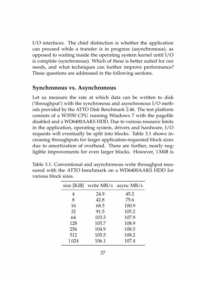
I/O interfaces. The chief distinction is whether the applicationcan proceed while a transfer is in progress (asynchronous), asopposed to waiting inside the operating system kernel until I/Ois complete (synchronous). Which of these is better suited for ourneeds, and what techniques can further improve performance?These questions are addressed in the following sections.

Synchronous vs. Asynchronous

Let us measure the rate at which data can be written to disk(‘throughput’) with the synchronous and asynchronous I/O meth-ods provided by the ATTO Disk Benchmark 2.46. The test platformconsists of a W3550 CPU running Windows 7 with the pagefiledisabled and a WD6400AAKS HDD. Due to various resource limitsin the application, operating system, drivers and hardware, I/Orequests will eventually be split into blocks. Table 3.1 shows in-creasing throughputs for larger application-requested block sizesdue to amortization of overhead. There are further, nearly neg-ligible improvements for even larger blocks. However, 1 MiB is

Table 3.1: Conventional and asynchronous write throughput mea-sured with the ATTO benchmark on a WD6400AAKS HDD forvarious block sizes.

size [KiB] write MB/s async MB/s

4 24.9 45.28 42.8 75.616 68.5 100.932 91.5 105.264 103.3 107.9

128 105.7 108.9256 104.9 108.5512 105.5 108.2

1 024 106.1 107.4

27

a reasonable cutoff point (c.f. Section 3.2). As found in previ-ous work [58], asynchronous writes are faster to converge to thedisk’s maximum throughput. This is because the disk controllercan immediately begin the next transfer after the previous onecompletes without requiring the application to first transition intokernel mode. Asynchronous I/O generally involves higher CPUoverhead [59][p. 381], especially on Windows, which only providesFast I/O driver entry points for synchronous I/O [60]. However,it has the major advantage of allowing the application to performwork (e.g. compression) while waiting on previous transfers. Wetherefore prefer it to the more commonly used synchronous accessmethod.

Block Size

We wish to maximize disk throughput while overlapping computa-tion with I/O. It is straightforward to interleave these two tasks bysplitting transfers into blocks. Computations can be carried out fora completed block while waiting for subsequent I/Os. The blocksize is bounded by the following considerations: Transfers arecarried out via Direct Memory Access hardware, which requirescontiguous physical memory. Drivers must therefore represent theapplication-provided memory buffer as a list of physical pages(scatter-gather list). These are stored in nonpaged pool – a smallmemory area set aside by Windows – and are therefore restrictedto 255 entries [61]. The resulting limit is 1 MiB given a 4 KiB pagesize. Although it is desirable to amortize system call overhead overlarge requests, those exceeding this limit incur additional over-head due to splitting. Conversely, there must be a minimum blocksize because the number of pending I/O requests may be finite.Windows also requires transfer sizes to be sector-aligned, and theAdvanced Format industry initiative [62] has introduced driveswith 4 KiB sectors, so we consider that to be the minimum. Ta-ble 3.2 shows the read and write throughputs measured by ATTO

28

on the previously mentioned HDD and a 128 GB Crucial C300Solid-State Disk (SSD) over this range of block sizes. Although

Table 3.2: Asynchronous read and write throughput [MB/s] mea-sured with ATTO on a WD6400AAKS HDD and C300 SSD forvarious block sizes.

size [KiB] HD write HD read SSD write SSD read

4 45.2 102.9 126.9 202.98 75.6 102.4 134.2 253.9

16 100.9 98.4 135.3 284.132 105.2 101.7 129.4 304.864 107.9 77.4 139.8 214.3128 108.9 77.7 142.1 326.6256 108.5 83.2 141.7 323.4512 108.2 83.6 141.3 325.8

1 024 107.4 83.8 140.5 326.6

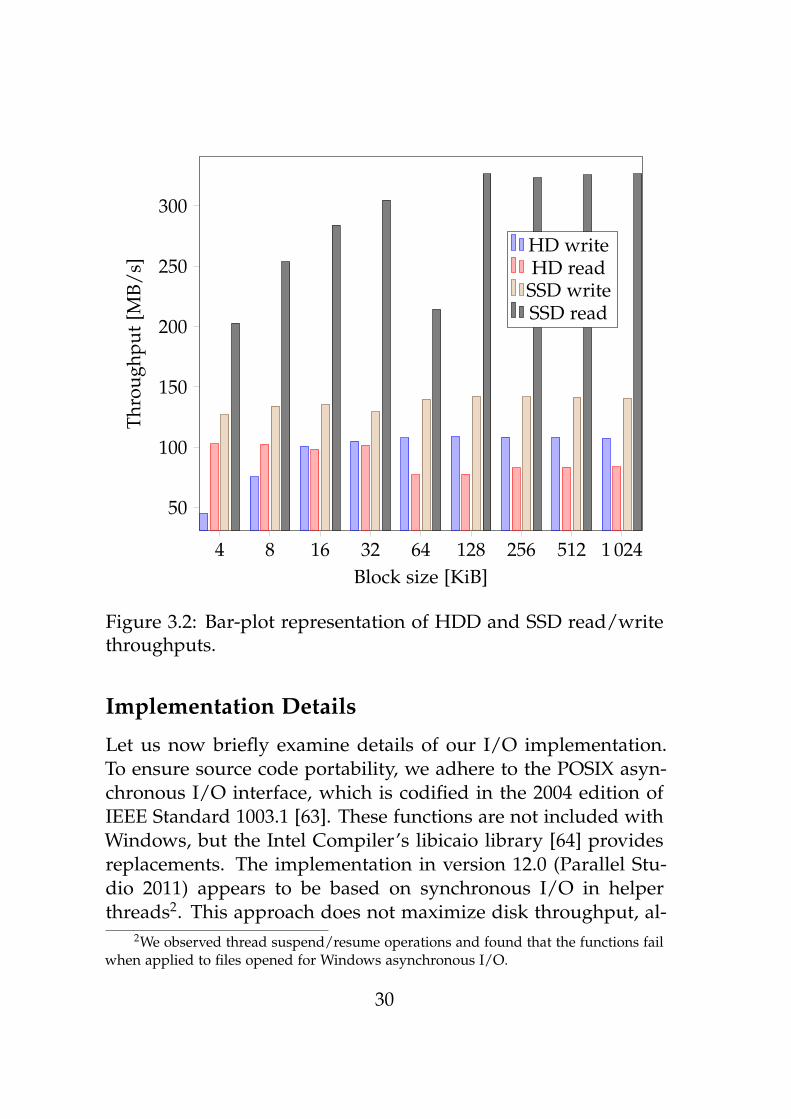
SSD read throughput tends to increase with larger block sizes,the bar plot representation of these numbers in Figure 3.2 makesapparent a sharp drop at 64 KiB. The cause is unclear; perhapstransfers are being split up due to scatter-gather list limitationsor other inefficiencies within the driver or controller. However,write throughputs remain nearly constant. Interestingly, HDDwrites can outperform reads due to caching by the controller. Wechoose 128 KiB blocks as a reasonable compromise that providesgood throughput without requiring large buffers that exceed theL2 cache size. Note that this discussion presumes sequential I/O,which is justified in Section 3.1. Random I/O may require largerblock sizes to amortize the cost of HDD ‘seeks’1.

1Repositioning the read/write head in preparation for reading or writing fromanother location.

29

4 8 16 32 64 128 256 512 1 024

50

100

150

200

250

300

Block size [KiB]

Thro

ughp

ut[M

B/s]

HD writeHD read

SSD writeSSD read

Figure 3.2: Bar-plot representation of HDD and SSD read/writethroughputs.

Implementation Details

Let us now briefly examine details of our I/O implementation.To ensure source code portability, we adhere to the POSIX asyn-chronous I/O interface, which is codified in the 2004 edition ofIEEE Standard 1003.1 [63]. These functions are not included withWindows, but the Intel Compiler’s libicaio library [64] providesreplacements. The implementation in version 12.0 (Parallel Stu-dio 2011) appears to be based on synchronous I/O in helperthreads2. This approach does not maximize disk throughput, al-

2We observed thread suspend/resume operations and found that the functions failwhen applied to files opened for Windows asynchronous I/O.

30

though it does avoid the restrictions mentioned below. We in-stead implement the POSIX functions in terms of Windows asyn-chronous I/O. This entails specifying FILE_FLAG_OVERLAPPEDand FILE_FLAG_NO_BUFFERING when opening the file. Win-dows then requires addresses, sizes and offsets to be a multi-ple of the volume sector size. Our low-level functions pass onthese constraints to their callers, which can handle them with-out penalty. Several lesser-known tricks [65] have also been ap-plied. Contiguous storage for OVERLAPPED structures, the Win-dows equivalent of POSIX aiocb (asynchronous I/O control blocks),allows pinning them in the kernel address space by means of theSetFileIoOverlappedRange API. This means I/O completioncan be handled by any thread, which avoids an asynchronous pro-cedure call and the associated context switch and locking in thekernel. SetFileCompletionNotificationModes is used toavoid unnecessary completion notifications. Finally, disk space ispreallocated via SetEndOfFile and SetFileValidData. With-out the latter, all writes that extend a file are forced to completesynchronously, which prevents overlapping I/O with computation(e.g. checksums) [66]. To avoid exposing previous disk contents,we deny read sharing when opening files.

Having gone to great lengths to ensure an efficient implemen-tation of the POSIX aio interface, the application logic is compar-atively simple. A ring buffer holds aiocb control blocks. BlockI/Os are issued up to a default maximum queue depth of 32. Weuse aio_suspend to wait until the next I/O is complete and theninvoke a user-specified callback (specified as a C++ function ob-ject template to avoid call overhead). The loop terminates whenall block I/Os have completed. The Windows alignment require-ments (similar considerations apply when using the equivalentLinux/BSD O_DIRECT functionality) are satisfied by the memoryallocator, which also expands block buffers to a multiple of thesector size. After writing, we trim any excess padding at the endof the file by calling truncate.

31

Throughput

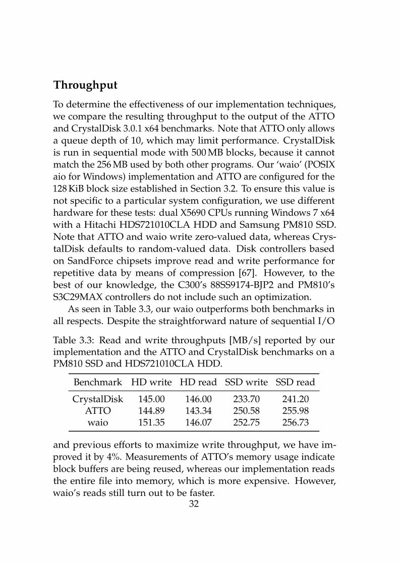
To determine the effectiveness of our implementation techniques,we compare the resulting throughput to the output of the ATTOand CrystalDisk 3.0.1 x64 benchmarks. Note that ATTO only allowsa queue depth of 10, which may limit performance. CrystalDiskis run in sequential mode with 500 MB blocks, because it cannotmatch the 256 MB used by both other programs. Our ‘waio’ (POSIXaio for Windows) implementation and ATTO are configured for the128 KiB block size established in Section 3.2. To ensure this value isnot specific to a particular system configuration, we use differenthardware for these tests: dual X5690 CPUs running Windows 7 x64with a Hitachi HDS721010CLA HDD and Samsung PM810 SSD.Note that ATTO and waio write zero-valued data, whereas Crys-talDisk defaults to random-valued data. Disk controllers basedon SandForce chipsets improve read and write performance forrepetitive data by means of compression [67]. However, to thebest of our knowledge, the C300’s 88SS9174-BJP2 and PM810’sS3C29MAX controllers do not include such an optimization.

As seen in Table 3.3, our waio outperforms both benchmarks inall respects. Despite the straightforward nature of sequential I/O

Table 3.3: Read and write throughputs [MB/s] reported by ourimplementation and the ATTO and CrystalDisk benchmarks on aPM810 SSD and HDS721010CLA HDD.

Benchmark HD write HD read SSD write SSD read

CrystalDisk 145.00 146.00 233.70 241.20ATTO 144.89 143.34 250.58 255.98waio 151.35 146.07 252.75 256.73

and previous efforts to maximize write throughput, we have im-proved it by 4%. Measurements of ATTO’s memory usage indicateblock buffers are being reused, whereas our implementation readsthe entire file into memory, which is more expensive. However,waio’s reads still turn out to be faster.

32

3.3 File Format

With the in-memory image representation and I/O method es-tablished, we may now decide upon the format of the files toread/write. A multitude of image file formats have been devised.However, our applications and large amounts of data impose exact-ing requirements, including minimal conversion overhead, supportfor relevant pixel formats, compression, tiling, ‘image pyramids’3

and flexible ‘metadata’4. Let us briefly review a selection of existingformats and evaluate them in light of these requirements:

PM is a simplistic format that only specifies one or more planes ofband-interleaved pixels without any additional features [68].Application-specific metadata could be stored in the free-form comment field, but we would prefer a standardizedapproach.

OpenEXR is a newer format for High Dynamic Range (HDR)images that unfortunately lacks support for 8 or 16-bit inte-gers [69].

HFA/IGE are the feature-rich internal file formats of the ERDASIMAGINE framework for geospatial image processing [70].However, the HFA format is quite complex and somewhatinefficient (c.f. Section 3.4).

NITF is a standardized interchange format that is even more com-plex than HFA, but limited to 10 GB and lacking supportfor embedded image pyramids. Note that NSIF (NATO Sec-ondary Image Format) corresponds to NITF with a differentversion field in the header. [71]

3A series of successively spatially subsampled versions of the image, also known asmipmaps. Subsequent to the ‘base’ (the original image), each ‘level’ typically halves theresolution. A viewer can reduce the overhead of ‘minifying’ many image pixels to fewscreen pixels by interpolating between the two levels whose resolutions are closest tothe desired zoom scale.

4Literally “data about data”, here understood to be additional information aboutthe image such as its geographic location.

33

BigTIFF expands the well-known TIFF format to 64-bit offsets [72],but inherits its major ‘disadvantage’ of allowing non-nativebyte orders and non-tiled pixel formats, which would requireexpensive conversion when loading.

Unfortunately, each of these formats is either prone to ineffi-ciency, or lacks some of the required features. We have devised aflexible new format designed with knowledge of low-level detailssuch as SIMD vector and disk sector alignment requirements. Itprovides support for tiled pyramids ordered according to a novelspace-filling curve, the new lossless compression scheme describedin Chapter 4, and user-defined metadata. Details are given inAppendix B.3. However, we recognize the value of interoperabilityand wish to support existing applications and viewers, particu-larly ERDAS IMAGINE. We therefore provide fast methods forwriting NITF and IGE files. The key enabling factor of their highperformance is assembling the file in memory and writing it todisk in large chunks. Avoiding unnecessary copying of the dataand additional allocations (e.g. for headers) also saves time.

3.4 Performance

Let us now study the real-world performance attained by themethods described in this chapter. We compare the total timerequired to write NITF and IGE images with our software and theubiquitous Geospatial Data Abstraction Library (GDAL), version1.7.3.

To avoid favoring a particular tile size, we generate images withrandom dimensions in the interval

[2i, 2i+1

)for 10 ≤ i < 15. The

resulting values are given in Table 3.4. Table 3.5 compares therelative costs of our NITF and IGE codecs vs. GDAL. The currentbalance of CPU performance and disk throughput means writingNITF images takes about 5–25% longer because pixels must be

34

Table 3.4: Randomly chosen image dimensions [pixels] for thewrite throughput test.

Dataset Width Height

0 1 140 1 9171 3 039 3 7522 8 084 7 5053 8 921 10 2514 24 608 19 359

Table 3.5: Normalized cost of the formats – elapsed times for NITFand IGE are divided by the I/O time, GDAL measurements arerelative to our implementation.

Drive Dataset NITF IGE GDAL NITF GDAL HFA

HD 0 1.62 2.61 3.97 3.84HD 1 1.12 1.36 5.55 5.82HD 2 1.05 1.47 5.34 5.06HD 3 1.07 1.41 5.44 5.42HD 4 1.12 1.49 5.90 3.20

SSD 0 1.42 2.50 4.31 5.19SSD 1 1.15 1.38 11.99 7.53SSD 2 1.24 1.45 6.88 7.45SSD 3 1.22 1.55 8.26 7.40SSD 4 1.20 1.35 7.53 4.04

reshuffled into a tiled layout5. The relative cost of this computationis higher on the smallest dataset because less time is required forI/O (possibly due to caching in the disk controller). Our IGEwriter performs much more work: computing and storing animage pyramid as well as statistics (standard deviation, minimum,

5Our normative reference for NITF is NATO Standardization Agreement 4545,which requires NSIF images with a dimension exceeding 8 192 pixels to be split intotiles. We use a fixed tile dimension of 256.

35

maximum, mean, median, mode and histogram of each band’svalues). This only requires 35–50% more time than I/O due toour efficient vectorized and parallelized implementation. However,the overhead appears particularly large on the smallest imagebecause the cost of writing the extra metadata file is not amortized.Our NITF implementation is roughly five times as fast as GDAL’swhen writing to the HDD, and up to 12 times as fast on the SSD(whose higher throughput increases the relative cost of GDAL’s lessefficient pixel copying). Our IGE writer is ‘only’ about 5 times asfast as GDAL on the HDD and 7 times as fast on the SSD becauseGDAL does not compute image statistics. For reasons unknown,GDAL’s throughput increases on the largest (3.8 GB) image. Thewidth is a multiple of 32, but a block size of 64 is used. Figure 3.3shows the speedups vs. GDAL. Although mere constant factors,we believe a 3 to 12-fold improvement to be of major practicalrelevance.

3.5 Conclusion

This chapter has described a technique for asynchronous I/O thatavoids various inefficiencies at the hardware/operating systemlevel, thereby outperforming existing benchmarks by 4%. We buildupon this foundation with efficient routines for writing commonimage file formats. The result is a 3 to 12-fold speedup vs. thewell-established GDAL library. Finally, the aligned image lay-out discussed herein serves to avoid penalties when accessingindividual rows via SIMD instructions, thus enabling the highperformance of the subsequent modules.

36

0 1 2 3 40

2

4

6

8

10

12

Dataset

Spee

dup

vs.G

DA

L

NITF (HD)NITF (SSD)IGE (HD)IGE (SSD)

Figure 3.3: Speedup of our writers vs. GDAL.

37

Chapter 4

Lossless Asymmetric SIMDCompression

This chapter introduces a new lossless asymmetric SIMD codec(LASC) designed for extremely efficient decompression of largesatellite images. A throughput in excess of 3 GB/s allows decom-pression to proceed in parallel with asynchronous transfers fromfast block devices such as disk arrays. This is made possible by asimple and fast SIMD entropy coder that removes leading null bits.Our main contribution is a new approach for vectorized predictionand encoding. Unlike previous approaches that treat the entropycoder as a black box, we account for its properties in the designof the predictor. The resulting compressed stream is 1.2 to 1.5times as large as JPEG-2000, but can be decompressed 100 times asquickly – even faster than copying uncompressed data in memory.Applications include streaming decompression for out of core vi-sualization. To the best of our knowledge, this is the first entirelyvectorized algorithm for lossless compression.

This chapter has been published in the “Software: Practiceand Experience” journal [73] and is reproduced here with minorformatting and wording clarifications.

39

4.1 Introduction and Related Work

Displaying images that are too large to fit within main memorynecessitates streaming, that is, loading sections of the data froma slower storage medium when they are needed. For interactiveperformance, it is important to minimize the latency of these re-quests. Asynchronous I/O allows computation to proceed whilewaiting on the storage medium. However, panning a 2 560× 1 600pixel viewport such that 10% of the 16-bit, four component pix-els are updated every 16 ms requires a sustained throughput of196 MB/s, which exceeds the capability of current magnetic me-dia [74]. Such data rates are enabled by drive arrays and top of theline solid-state disks, but these are not always available. Instead,a common remedy involves compression of the data. In contrastto the entertainment sector, some medical and automated imageanalysis applications cannot tolerate any loss of information.

Lossless Image Compression

By 1993, a general framework for lossless image compression hadbeen established that is still useful today. The intensity of thenext pixel to encode is predicted using a context of previouslyseen pixels. The resulting residuals, that is, prediction errors, arerelayed to a statistical coder that may act upon knowledge of theirdistribution [75]. These components are all interdependent; webriefly discuss them in increasing order of complexity. In mostcases, the simple and intuitive raster scan order is used. Surpris-ingly, the order induced by a Hilbert space-filling curve can increasethe residuals’ entropy [76], and the ‘rain scan order’ only yieldsa 4% improvement [77]. The circular dependency between pre-diction and coding is often resolved by assuming that predictionerrors follow a Laplacian distribution [78], for which a variantof Golomb coding is optimal [79]. With the entropy coder thusestablished, most efforts have been directed at prediction – using

40

larger contexts [80], combining various predictors [77] or minimiz-ing the squared or absolute prediction error [81]. However, thisdoes not necessarily result in optimal compressed sizes [82], andconventional entropy coders are too slow for our application. Ahighly-optimized implementation of Rice’s independently discov-ered subset of Golomb codes only decodes 200 MIntegers/s [83].Prior work on reducing branches in a Huffman decoder reached90.95 MPixel/s (including a fast DCT) [84]. However, this algorithmis not well-suited for acceleration via GPU, which only manages570–750 MB/s [85]. Note that Huffman codes are equivalent toa restricted case of arithmetic coding [86], so the latter cannot beexpected to be faster. Dictionary-based approaches are neither sig-nificantly better in terms of performance [87], nor are they ideallysuited for this task because residuals are not drawn from a smallalphabet.

Entropy Coding

Having ruled out conventional entropy coders, we must consider al-ternatives. Variable-length codes are generally inefficient to decodebecause of their bit-level accesses, and even table-based approachesare not much faster [88]. We therefore turn to fixed-length codes.One interesting approach involves packets of compressed fields anda selector indicating their length [89]. Recently, a similar schemeusing 64-bit words with support for values spanning multiple pack-ets was also proposed [90]. These are faster than variable-lengthcodes and improve upon the compression of byte-aligned codes,but suffer from several drawbacks. Extracting the fields still re-quires bit arithmetic. The varying number of output values perpacket complicates single instruction multiple data (SIMD) writes.A single large residual increases the size of all fields in the packet.The latter issue can be addressed by storing ‘exceptions’, that is,a list of values to overwrite after decompression and their loca-tions [91]. However, this is unlikely to be useful for 16-bit values

41

because the reduction in size for small packets is roughly equalto the encoded size of an exception. The main aspect of the pre-viously cited work is optimization for superscalar processors thatcan execute more than one instruction per clock cycle. Whereasthis enables a throughput of 1 GB/s, we believe the key to fullyutilizing modern CPUs lies in SIMD. Recently, two such schemesfor compression by omitting the most-significant zero-valued bits(null suppression [92]) have been introduced. The first [93] usesmultiplication and complex alignment logic for SIMD extractionof variable-length fields, which restricts it to 32-bit values due tolimitations in the instruction set. The second approach [94] relieson a new instruction for permuting bytes, which requires relativelylarge lookup tables and is unable to compress fields to less than8 bits. In Section 4.2, we describe a surprisingly simple but fasteralternative that is also suitable for 16-bit pixels and requires noadditional memory.

Asymmetric Compression

Our primary focus is on decompression speed, which must matchthe throughput of high-end solid-state disks. We are willing toaccept an asymmetric coder/decoder (codec) that spends moretime on compression, because large datasets usually require con-siderable time to generate anyway. Ideally, the offline encoderwould choose the best predictor for each pixel. Despite potentiallyreducing the encoded size of the prediction errors, the savingsare unlikely to exceed the cost of transmitting so much additionalinformation to the decoder. This overhead can be greatly reducedby quantizing predictor vectors to a ‘codebook’ of frequently usedentries [82]. The high computational cost of this method can bereduced by predicting entire 2-D blocks of pixels, similar in prin-ciple to video motion compensation. A recent approach employsa brute-force search for matching blocks [95]. The compressiontime is reduced by resorting to CALIC’s prediction of individual

42

pixels [96] in smooth image regions. However, even a simple func-tion of neighboring pixels is relatively costly for the decoder tocompute. We propose to eliminate this step entirely and rely uponefficient SIMD matching in a sliding window to maintain accept-able compression throughput. To further speed up the algorithm,we deal with 1-D tuples (as many pixels as will fit in a SIMD reg-ister) instead of 4× 4 blocks. In contrast to previous approaches,the predictor is designed with full knowledge of the subsequententropy coder. Section 4.3 introduces our new algorithm, whichwe believe to be the first SIMD sliding window compressor. Theresult is a twofold reduction in image size with decompressionthat outperforms a state-of-the-art integer coder [94].

4.2 Fast SIMD Integer Packing

Let us define packing as reducing an n bit two’s complement rep-resentation of a value in

[−2m−1, 2m−1

)to m bits, as shown in

Figure 4.1. This section addresses the question of how to pack

FFF8

8

0000

0

FFFF

F

0002

2

0007

7

FFF9

9

Figure 4.1: Hexadecimal representation of six n = 16 bit values,each packed into m = 4 bits by omitting the 12 most significant bitsbecause they carry no information.

(and conversely ‘unpack’) tuples of values as quickly as possibleusing the ubiquitous SSE2 instruction set [97]. In fact, our terminol-ogy derives from its mnemonics, which include PACK instructionsfrom n ∈ 16, 32 to m = n/2 and UNPCK instructions that inter-leave m bit values for purposes of sign- or zero-extension. Withtheir aid, two- and fourfold packing/unpacking of 32-bit values

43

is straightforward. The latency of two back-to-back pack/unpackinstructions is higher than a single PSHUFB universal shuffle, butthe more recent SSE4.1 instruction set provides for sign-extending8-bit values to 16 or 32 bits via PMOVSX. Both methods avoid theneed for loading shuffle control masks from memory, and moreimportantly, allow m < 8. For example, we can unpack from m = 4to n = 16 as expressed by the following intrinsics1:

typedef __m128i V;V hi_lo16 = _mm_unpacklo_epi8(in, in);V lo16 = _mm_slli_epi16(hi_lo16, 4);V left16 = _mm_unpacklo_epi16(lo16, hi_lo16);return _mm_srai_epi16(left16, 12);

The final arithmetic right shift sign-extends the values to 16-bits.Packing from n = 16 to m = 4 is somewhat more involved:

typedef Iu16vec8 V;V zero = _mm_setzero_si128();V values8 = _mm_packs_epi16(values, zero);V hi = (values8 & _mm_set1_epi16(0x0F00)) >> 4;V lo = (values8 & _mm_set1_epi16(0x000F));return _mm_packus_epi16(hi | lo, zero);

The latter code uses the more convenient notation afforded by C++vector classes with operator overloading. Similar functions forpacking/unpacking of other data types are expressed as templatespecializations so that their caller can simply invoke, for examplePack2x without any additional type dispatching.

1Functions built into three major C++ compilers (GCC, Intel and Microsoft) thatgenerate SIMD instructions while relieving the programmer of instruction schedulingand register allocation.

44

4.3 SIMD Sliding-Window Compression

We now derive a codec designed for an extremely high decompres-sion throughput while retaining a reasonable compression ratio.Our chief interest lies in compressing high-resolution satellite im-ages, which typically consist of 4 or 8 spectral bands of 16-bitsamples. The bands are often interleaved by pixel, for example,Blue0 Green0 Red0 NIR0, Blue1 Green1 Red1 NIR1, · · ·, where NIR isthe near-infrared spectral band. Because inter-band correlationis weaker than spatial correlation [98], and interleaved pixels canmore readily be displayed by graphics hardware, we avoid con-verting to a planar representation. The raw data is not amenableto null suppression, so we combine the previously introduced en-tropy coder with a predictor. Making full use of the transistors inmodern CPUs requires SIMD processing. However, even compar-atively simple predictors such as LOCO-I [99] are not suitable inthis regard because they access multiple (unaligned) neighbors. Weinstead predict a tuple of values from a single previous (aligned)tuple. This is effective at reducing spatial redundancy, but assumesthat the number of bands evenly divides the SIMD width. Imagesobtained via synthetic aperture radar, laser scanners and currenthigh-resolution imaging satellites meet this requirement. Other-wise, prediction would rely on the weaker inter-band correlation. Itis too expensive to encode an offset for each tuple, so we combinethem into larger units called ‘blocks’ (not to be confused with the2-D blocks in [95]). Because these are always accessed as a unit, wedefine them to match the L1 cache line size.

What we have, thus far, is a block of values and a previousblock as a frame of reference. In contrast to PFOR [91], eachcomponent of a pixel has its own reference value. How, then,is the reference block to be chosen? It is here that we tailor thepredictor to fit the entropy coder. Because our maximum packingof n = 16 bit prediction errors allows for the m = 4 bit interval[−8, 8), it would be misleading to minimize the sum of absolute

45

prediction errors as in [95]. Instead, we define the goal function asthe actual packed size of the block for a given choice of referenceblock. This directly minimizes the compressed size instead of justassuming the entropy coder will handle ‘small’ prediction errorsefficiently. The packed size is computed by checking whether alln bit values in a tuple can be packed into m = n/2 or n/4 bits(that is, whether each value plus 2n−1 is zero when shifted rightby m bits). This biased representation of signed numbers allowshardware-assisted decoding via right arithmetic bit shifts, unlikethe ‘sign in the lowest bit’ encoding [100]. Our search for thereference block yielding the smallest packed size breaks ties in favorof the most recent block, which is less likely to have been evictedfrom the decoder’s cache. To further improve temporal locality,we restrict the search to a sliding window of the previous outputs.Note the resulting similarity to the Lempel-Ziv family of adaptivedictionary coders, with the distinction that our matches are fixed-length (helpful for SIMD) and approximate (due to the propertiesof the subsequent entropy coder). Larger sliding windows allowadditional matches but decrease encode throughput. We willexamine this trade-off in Section 4.4.

It remains to be seen how the decoder is notified of the tuples’packing. To maintain the word-alignment of the encoded stream,which avoids microarchitecture-specific penalties2, we combineseveral blocks into a ‘group’ described by a word-sized header.However, binary encodings of three values (two- or fourfold pack-ing and uncompressed) are wasteful or slow. Because it is rare toencounter a block for which no similar blocks exist, we requireall tuples within such blocks to be stored uncompressed. This iscommunicated by an illegal value (0) for the reference block’s offset.Otherwise, a bit field indicates which tuples in a block are packedby a factor of four. To reduce the number of conditional branches

2Unaligned memory accesses that straddle a cache line or page boundary mayincur significant delays depending on the CPU. For example, the Intel Core 2 appearsto bypass the L1 cache and TLB in such cases (c.f. Section B.2).

46

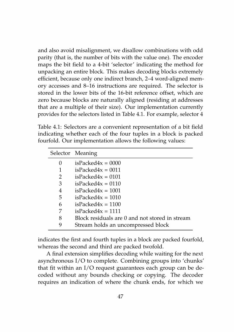
and also avoid misalignment, we disallow combinations with oddparity (that is, the number of bits with the value one). The encodermaps the bit field to a 4-bit ‘selector’ indicating the method forunpacking an entire block. This makes decoding blocks extremelyefficient, because only one indirect branch, 2–4 word-aligned mem-ory accesses and 8–16 instructions are required. The selector isstored in the lower bits of the 16-bit reference offset, which arezero because blocks are naturally aligned (residing at addressesthat are a multiple of their size). Our implementation currentlyprovides for the selectors listed in Table 4.1. For example, selector 4

Table 4.1: Selectors are a convenient representation of a bit fieldindicating whether each of the four tuples in a block is packedfourfold. Our implementation allows the following values:

Selector Meaning

0 isPacked4x = 00001 isPacked4x = 00112 isPacked4x = 01013 isPacked4x = 01104 isPacked4x = 10015 isPacked4x = 10106 isPacked4x = 11007 isPacked4x = 11118 Block residuals are 0 and not stored in stream9 Stream holds an uncompressed block

indicates the first and fourth tuples in a block are packed fourfold,whereas the second and third are packed twofold.

A final extension simplifies decoding while waiting for the nextasynchronous I/O to complete. Combining groups into ‘chunks’that fit within an I/O request guarantees each group can be de-coded without any bounds checking or copying. The decoderrequires an indication of where the chunk ends, for which we

47

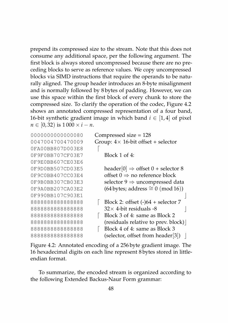
prepend its compressed size to the stream. Note that this does notconsume any additional space, per the following argument. Thefirst block is always stored uncompressed because there are no pre-ceding blocks to serve as reference values. We copy uncompressedblocks via SIMD instructions that require the operands to be natu-rally aligned. The group header introduces an 8-byte misalignmentand is normally followed by 8 bytes of padding. However, we canuse this space within the first block of every chunk to store thecompressed size. To clarify the operation of the codec, Figure 4.2shows an annotated compressed representation of a four band,16-bit synthetic gradient image in which band i ∈ [1, 4] of pixeln ∈ [0, 32) is 1 000× i− n.

000000000000008000470047004700090FA00BB807D003E80F9F0BB707CF03E70F9E0BB607CE03E60F9D0BB507CD03E50F9C0BB407CC03E40F9B0BB307CB03E30F9A0BB207CA03E20F990BB107C903E1888888888888888888888888888888888888888888888888888888888888888888888888888888888888888888888888

Compressed size = 128Group: 4× 16-bit offset + selectord

Block 1 of 4:

header[0]⇒ offset 0 + selector 8offset 0⇒ no reference blockselector 9⇒ uncompressed data(64 bytes; address ∼= 0 (mod 16))

cd Block 2: offset (-)64 + selector 7

32× 4-bit residuals -8 cd Block 3 of 4: same as Block 2

(residuals relative to prev. block)cd Block 4 of 4: same as Block 3

(selector, offset from header[3]) cFigure 4.2: Annotated encoding of a 256 byte gradient image. The16 hexadecimal digits on each line represent 8 bytes stored in little-endian format.

To summarize, the encoded stream is organized according tothe following Extended Backus-Naur Form grammar:

48

Stream = Chunk-;Chunk = CompressedSize, Group-, ChunkPadding;CompressedSize = Bit*64;ChunkPadding = Bit*8 (* < 128 KiB *);Group = GroupHeader, PackedBlock*4;GroupHeader = Match*4;Match = Offset, Selector (* added together *);(* offsets are multiples of 16 bytes *)Offset = Bit*16 (* backwards distance *);Selector = Bit*4 (* see Table I *);PackedBlock = PackedTuple*4;(* omitted if selector = 8 *)PackedTuple = ‘packed 1x|2x|4x’;Bit = ‘unsigned integer bit’;

4.4 Measurements

This section presents measurements of the speed and compres-sion ratio of our new algorithm for purposes of comparison withexisting approaches.

Hardware and Software

The test platform consists of dual W5580 CPUs (3.2 GHz) run-ning Windows XP x64, 48 GiB DDR3-1066 memory and an80 GB Fusion IO card. Our implementation is compiled withICC 12.0.1.096 /Ox /Ob2 /Oi /Ot /GA /GR- /GS- /Gy /EHsc /MD

/Qipo /QxSSE4.1 /Qopenmp /Qstd=c++0x. We use lossless JPEG-2000 and Lempel-Ziv Markov chain compression as a basis forcomparison. The former is provided by GeoJasper 1.3.1 [101], com-piled with nearly identical settings (our algorithm is not influencedby string merging nor floating-point arithmetic, but we enable /GF

/fp:fast=2 for GeoJasper while omitting /Qopenmp /Qstd=c++0x,

49

because it does not use those features). LZMA is represented bythe public 64-bit release of 7-Zip, version 9.2 [102]. Both of thesealgorithms are run with their default parameters.

Datasets

The codec is primarily intended for compression of images withfour 16-bit bands. We arbitrarily chose four pan-sharpened [103]satellite datasets and extracted subsets of increasing size basedon the interesting areas in the image. Each contains a mix ofurban and natural terrain (Figure 4.3). A 16-bit panchromaticQuickbird image of Frankfurt, Germany, is also included. Because

Figure 4.3: Screen capture of 16-bit, 4 channel subsets of pan-sharpened Quickbird images. Clockwise from top left: Wangen(Switzerland) and Neureut, Dorsten, Ettlingen (Germany). Copy-right DigitalGlobe Incorporated.

50

8-bit and/or RGB images are in widespread use, we implementa preliminary test that zero-expands the pixels to 16-bit, adds afourth component, and then applies the same codec. Searchingfor large, publicly available images, we found two 8-bit grayscalelunar mosaics [104, 105], two large images (hs-1999-14-b and hs-2004-52-a) from the Hubble spacecraft, two mosaics of the StanfordMemorial Church [106], and the PIA13804 panorama from theMars Phoenix lander. Their dimensions and format are listed inTable 4.2.

Table 4.2: Test images and their abbreviated identifiers, dimensions,number of bands and bit depth.

Dataset ID Width Height Bands Bits

QB Wangen QW 2 274 1 123 4 16QB Neureut QN 3 735 2 230 4 16QB Ettlingen QE 5 808 3 692 4 16QB Dorsten QD 7 232 6 029 4 16

QB Frankfurt QF 10 336 10 520 1 16LunarMosaic1 LM1 11 000 11 000 1 8LunarMosaic2 LM2 24 000 24 000 1 8

Hubble1 H1 4 189 2 624 1 8Hubble2 H2 4 136 3 813 3 8

MemChuNight MCN 11 184 7 456 3 8MemChu MC 16 965 8 230 3 8PIA13804 P1 26 180 6 180 3 8

Throughput

After loading the pixels in 256 × 256 band-interleaved tiles bymeans of the GDAL library [107], we measured the in-memoryencode and decode throughputs on a single CPU core (Table 4.3).The latter varies between 2 600 and 3 000 MB/s, which exceeds

51

Table 4.3: Single-threaded encode/decode throughput for tiledimages.

Dataset Encode MB/s Decode MB/s

QB Wangen 230.61 2 650.22QB Neureut 192.41 2 701.95QB Ettlingen 191.40 2 750.07QB Dorsten 165.11 2 674.20

QB Frankfurt 207.13 2 828.23LunarMosaic1 198.68 2 995.02LunarMosaic2 194.11 2 953.05

Hubble1 241.77 2 689.83Hubble2 168.74 3 033.28

MemChuNight 171.29 3 044.30MemChu 189.66 3 132.61PIA13804 165.95 3 070.56

our design goal of keeping up with a 16-drive array (1 GB/s) andFusion-io Duo (1.4 GB/s). Decompression is 13 to 18 times as fast ascompression, underscoring the asymmetric nature of the algorithm.Both compression and decompression throughput increases whenthe image contains more homogeneous regions.

For a fair comparison with the times reported by GeoJasper’s-verbose mode, we also write and read the encoded data to/fromdisk. Decoding is overlapped with asynchronous reads. Theresulting elapsed times and speedups vs. GeoJasper are shown inTable 4.4. LASC compression is 13 to 20 times as fast as JPEG-2000on the four-band datasets, and decompression is more than 100times as fast.

Because the 7-Zip executable lacks instrumentation, we recordits total execution time and therefore also include I/O in the LASCtimings. Tiles are read from image files by means of the GDALlibrary, which is not optimized for speed and falls far short of the

52

Table 4.4: Elapsed times [s] for compressing data from memoryand decompressing from file and the speedup vs. GeoJasper (GJ).

Dataset Encode+I/O vs. GJ I/O+Decode vs. GJ

QB Wangen 0.117 20.4 0.018 114.6QB Neureut 0.472 14.8 0.062 100.0QB Ettlingen 1.058 19.4 0.166 111.5QB Dorsten 2.385 13.3 0.274 103.4

QB Frankfurt 1.221 16.5 0.199 88.1LunarMosaic1 1.294 8.3 0.136 69.6LunarMosaic2 6.559 13.0 0.885 85.9

Hubble1 0.109 9.3 0.013 63.7Hubble2 0.842 8.2 0.083 72.3

MemChuNight 4.286 5.0 0.424 46.4MemChu 6.478 5.3 0.695 45.4PIA13804 8.674 6.2 0.883 52.4

disk throughput. However, as shown in Table 4.5, LASC compres-sion is still between 33 and 72 times as fast as 7-Zip on the satellitedata. There is less of a speedup on the other datasets because weexpanded them to 16-bit and/or four bands. However, for reasonsunknown, 7-Zip is also surprisingly efficient on the Hubble andMemChu datasets. LASC decompression is 15 to 20 times as faston the multispectral datasets. Note that the LZMA algorithm ispartially parallelized, whereas the above LASC results are for a sin-gle core. This is important because 60% of surveyed PCs are single-or dual-core [108]. However, more cores might be available forcompression, so we process tiles in parallel. This enables a through-put of 1 212.46 MB/s on the Ettlingen dataset and 1 122.01 MB/s onDorsten. Because tiles are tightly-packed within the output stream,each thread must encode into a temporary buffer and later copyit to the destination. This additional overhead explains why theeight cores only achieve a respective speedup of 6.3 and 6.8 oversingle-threaded compression. We have not implemented parallel

53

Table 4.5: Elapsed times [s] for compressing and decompressingfiles and the speedup vs. 7-Zip (7z).

Dataset Encode+I/O vs. 7z I/O+Decode vs. 7z

QB Wangen 0.211 35.8 0.048 20.8QB Neureut 0.935 33.4 0.151 17.4QB Ettlingen 1.654 49.5 0.393 16.9QB Dorsten 3.521 44.5 0.731 15.2

QB Frankfurt 1.558 72.1 0.484 12.3LunarMosaic1 2.362 29.4 0.441 6.9LunarMosaic2 11.247 19.0 2.332 10.1

Hubble1 0.311 1.9 0.044 8.5Hubble2 1.805 1.9 0.251 7.4

MemChuNight 7.243 9.1 1.289 4.3MemChu 11.237 6.2 2.144 4.3PIA13804 14.038 15.6 2.573 6.7

decompression because the single-core throughput already vastlyexceeds the I/O bandwidth on our system.

Compression Ratio

Whereas the algorithm is certainly fast, its usefulness hinges on rea-sonable compression ratios. Table 4.6 lists the resulting sizes aftercompressing each image with the three contenders. The bar-plotrepresentation of the compression ratios in Figure 4.4 puts thesenumbers in perspective. LASC is between 1.2 and 1.5 times as largeas JPEG-2000 on the multispectral satellite images that were ourprimary focus. We believe these results are applicable to other im-ages of the same pixel format, provided they possess a reasonabledegree of spatial redundancy. Random images with uncorrelatedpixels are, of course, incompressible. Our algorithm also appearssuitable for compressing some grayscale images, even 8-bit, withresults between 1.59 and 1.92 times as large as JPEG-2000. However,

54

QW QN QE QD QF LM1 LM2 H1 H2 MCN MC P1

0.39

0.34

0.41

0.29 0.290.25

0.46

0.24

0.45

0.240.2

0.33

0.41

0.46 0.46

0.31

0.380.35

0.53

0.32

0.53

0.3 0.29

0.470.470.5 0.51

0.38

0.47 0.48

0.72

0.42

0.82

0.72

0.66

0.85

Dataset

Com

pres

sion

Rat

io

JP2K LZMA LASC

Figure 4.4: Bar plot of JPEG-2000, LZMA and LASC compressionratios (compressed divided by original size) on all datasets, whoseabbreviations are defined in Table 4.2.

55

Table 4.6: Compressed sizes [bytes] for lossless JPEG-2000, 7-ZipLZMA and LASC.

Dataset JP2K LZMA LASC

QB Wangen 7 943 805 8 394 604 9 520 256QB Neureut 22 404 146 30 579 292 33 274 056QB Ettlingen 70 959 054 78 730 161 86 682 152QB Dorsten 100 733 299 108 713 351 134 249 560QB Frankfurt 63 273 877 81 755 880 102 217 840LunarMosaic1 30 277 033 41 976 100 58 110 352LunarMosaic2 262 841 520 304 749 383 417 357 096Hubble1 2 636 372 3 552 316 4 652 632Hubble2 21 475 077 24 870 958 38 893 272MemChuNight 59 279 177 74 055 192 179 736 160MemChu 84 643 231 119 494 493 274 525 352PIA13804 161 150 453 226 358 586 413 182 168

note that all of these images contain no-data regions in the corners,which results in space savings of 12 to 34.2% due to the additionalall-zero-residual selector. The right half of the plot clearly showsthe shortcomings of our preliminary approach that expands RGBto four components. It is actually surprising that compression wasattained despite having expanded the original data by a factor of2.6. The future work section proposes an approach for avoidingthis overhead. As it is, the algorithm typically results in a two-foldreduction of multispectral data; grayscale images may be reducedby a factor between 1.4 and 2.4.

Further Experiments

Table 4.7 shows the increase in compressed size of the Neureutimage for various tile dimensions. Given a 16 KiB sliding window,the largest tile size (512× 512) allows access to 512× 4 neighboringpixels – an imbalance that noticeably impacts compression. The

56

Table 4.7: Increase in compressed size for various tile dimensionscompared to the baseline of 256.

tileDim ∆ size

64 14.2%128 0.2%256 0.0%512 10.0%

smallest (64× 64) tiles provide a 64× 32 window, which is ap-parently too narrow to exploit much of the horizontal correlationin the image. To better understand these effects, we measuredthe distribution of match offsets (Figure 4.5) with a tile size of256× 256. The left and upper neighbors of the current block arethe most commonly used. However, about 1/3 of the blocks are acloser match with other blocks on the same line, thus underscoringthe importance of arbitrary offsets. Because previous lines are notreferenced as often, we restrict the sliding window to 2 KiB (thesize of a tile line). Each halving of the original 16 KiB size nearlydoubled encode throughput while increasing size by about 0.7%.

4.5 Conclusion

This chapter demonstrates the feasibility of lossless asymmetricSIMD compression (LASC). We propose a new entropy coder basedon null suppression via PACK instructions. Despite its simplic-ity, this approach enables a higher throughput than two recentlyproposed SIMD integer codecs and is not limited to 32-bit datatypes. A novel predictor designed with full knowledge of the coderreduces the spatial and intra-band redundancy of band-interleavedpixels. We avoid intricate computation and accesses to multipleneighboring values, instead predicting entire tuples of values bymeans of component-wise subtraction from a previous tuple. The

57

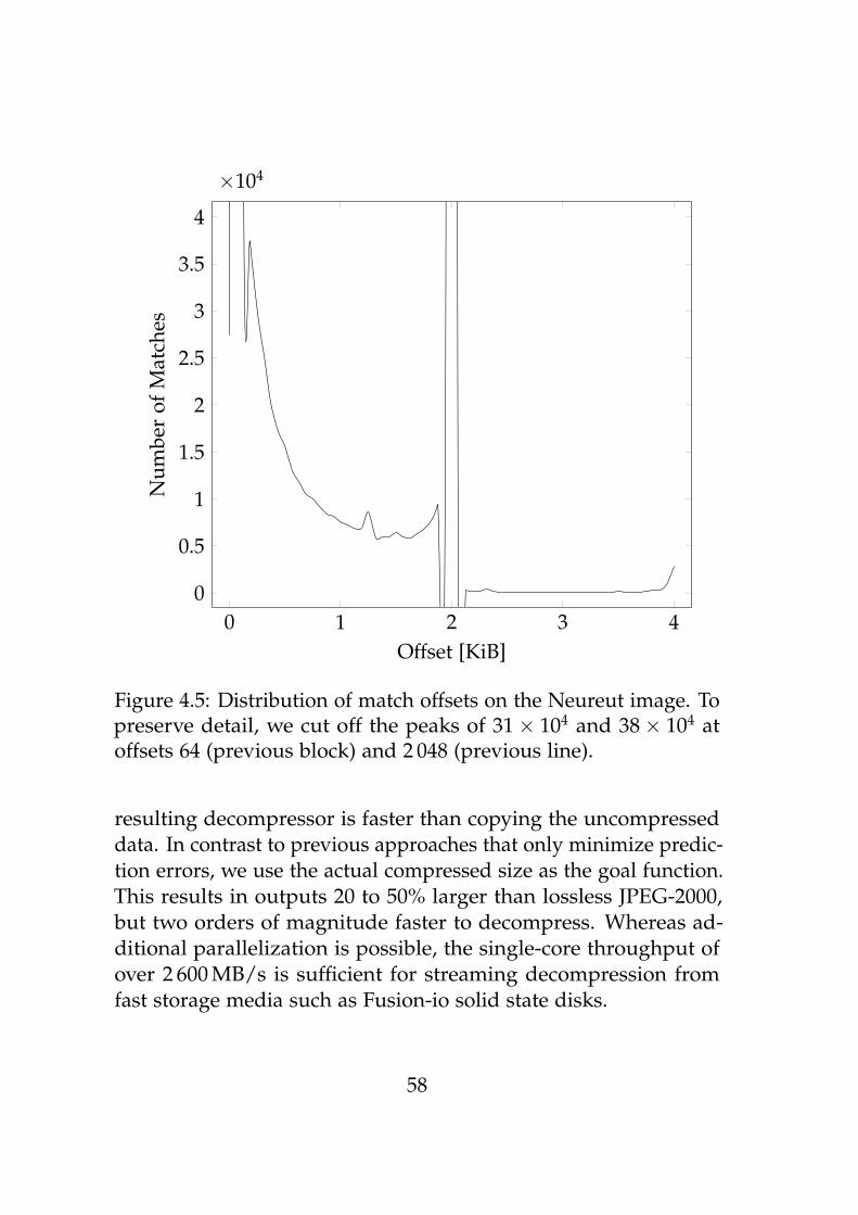
0 1 2 3 40

0.5

1

1.5

2

2.5

3

3.5

4

×104

Offset [KiB]

Num

ber

ofM

atch

es

Figure 4.5: Distribution of match offsets on the Neureut image. Topreserve detail, we cut off the peaks of 31× 104 and 38× 104 atoffsets 64 (previous block) and 2 048 (previous line).

resulting decompressor is faster than copying the uncompresseddata. In contrast to previous approaches that only minimize predic-tion errors, we use the actual compressed size as the goal function.This results in outputs 20 to 50% larger than lossless JPEG-2000,but two orders of magnitude faster to decompress. Whereas ad-ditional parallelization is possible, the single-core throughput ofover 2 600 MB/s is sufficient for streaming decompression fromfast storage media such as Fusion-io solid state disks.

58

Future Work. Our LASC algorithm enables extremely fast com-pression and especially decompression, but many avenues for im-proving its compression remain to be explored. We currently avoidtransmitting all-zero blocks, but extending this to individual tuplesshould improve compression of synthetic images, which often con-tain exact matches. Ideally, any combination of uncompressed, all-zero, two- and fourfold packed tuples would be allowed. Because44 selectors overly burden the CPU’s indirect branch predictor, theencoder can indicate which subset is the most useful for a par-ticular input dataset. A similar analysis of which reference blockoffsets are the most frequent could enable a smaller encoding of thematches, significantly speed up the compressor (by checking thoseoffsets first) and also reduce cache evictions in the decompressor. Ifthe encoder explicitly models these evictions, the sliding windowcould be enlarged (thereby improving compression) without anycost to the decoder. The resulting increase in compression timecan be reduced by means of a constant-time search for previousmatching blocks, for example, via hashing. Three-component RGBimages, for example, from digital cameras, currently require in-troducing an additional band, which increases the compressedsize by a factor of about 7/6. This overhead could be avoidedby storing an integral number of RGB triplets in each block andtemporarily expanding them to a four-component representationin the predictor. Finally, the codec should be evaluated for datatypes other than 16-bit values. Adding support for 32-bit integers(useful for document indexing or images from laser scanners) isstraightforward. Null suppression of floating-point data is alsochallenging, but it may be helpful to XOR the representations ofthe current and previous values [109].

59

Chapter 5

Pan Sharpening

Imaging satellites typically capture separate high-resolutionpanchromatic and lower-resolution multispectral datasets. Combin-ing them into a single ‘pan-sharpened’ image provides subsequentimage analysis tasks with color and structural information. Thistopic has been the focus of extensive research. However, personalcommunication indicating the operations of an international agencyare limited by the speed of its pan-sharpening software has moti-vated the development of a much faster algorithm. We build uponthe ‘Fast IHS’ technique, using a weighted linear combination ofthe upsampled multispectral bands to derive a composite imagecloser to what the panchromatic sensor had seen. The difference tothe actual panchromatic image approximates the high-frequencydetail signal and is injected into the multispectral bands. However,the fixed band weights typical of previous commercially availablealgorithms cannot account for differing atmospheric conditions.To further reduce color distortion, we compute the optimal bandweights for a given data set in the sense of minimizing the mean-square difference between the composite and panchromatic images.Because the (possibly multiplicative) noise in the panchromatic im-age impairs the subsequent graph-based segmentation algorithmdescribed in Chapter 6, an additional denoising step is appliedbefore fusion. We introduce an improved approximation of theBilateral Filter, which preserves edges and requires only one fast it-eration. Both algorithms are shown to be extremely efficient – large

61

satellite images can be processed within seconds. The quality of thefused image is evaluated in a comparative study of pan-sharpeningalgorithms available in ERDAS IMAGINE 9.3. Objective metricssuch as the ‘Q4’ quality index show improvements in color fidelity.

This chapter is a major revision of a contribution to the EarthResources and Environmental Remote Sensing/GIS Applicationsconference, co-authored by S. Laryea [103].

5.1 Introduction and Related Work

Imaging satellites such as IKONOS provide panchromatic (pan)imagery with sub-meter resolution [110]. However, segmenta-tion benefits from multispectral (MS) information [111]. Limitingphotons to individual bands requires larger detectors, so the MSresolution is typically between two and five times as coarse. In thecommon case where the satellite records both panchromatic andMS images, they can be fused into a high-resolution output thatalso includes color information. This is called resolution mergeor ‘pan sharpening’ (PS), for which many approaches have beenproposed. The popular IHS approach involves transforming colorsto Intensity, Hue and Saturation. Principal Component Analysis(PCA) and the related Gram-Schmidt transformation are examplesof statistical approaches. The Brovey transformation and wavelet-based techniques are examples of numerical methods. Finally,the Ehlers approach is a combination of IHS with Fast FourierTransform-based prefiltering [112].

Each of the previously mentioned algorithms have limitationsor drawbacks. A common problem relates to color distortion vs.the original MS image, which is caused by the spectral mismatchbetween the pan and MS bands. The IHS and PCA methods are par-ticularly vulnerable, because they replace a transformed band withthe original pan image. The mismatch can be reduced somewhat byequalizing the pan histogram before merging [113]. Another prob-lem relates to the sensor’s spectral response function. In the case of

62

the IKONOS satellite, the pan band extends past the NIR frequen-cies (c.f. Figure 5.1). Because the basic IHS transform ignores the

Figure 5.1: IKONOS spectral response function [114]. Note that Panextends beyond NIR, and that Blue and Green have a significantoverlap.

NIR band entirely, colors are perceived as distorted, especially inregions with green vegetation [115]. Weighting the MS bands canmostly compensate for this effect [116]. However, knowledge of thesensor’s spectral response is required, and fixed weights cannotaccount for changes in viewing conditions [117]. Whereas Earthobservation satellites often operate in sun-synchronous orbits [110],such that each pass occurs at the same local solar time, differencesin atmospheric conditions may still affect the spectral response.We avoid these issues by estimating the optimal weights for eachinput image, as discussed in Section 5.2. The quality metrics inSection 5.5 indicate this decreases the color distortion.

63

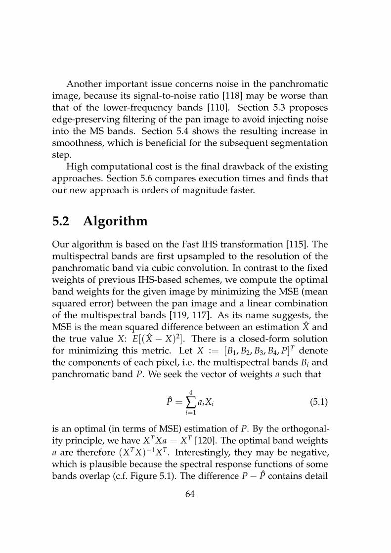
Another important issue concerns noise in the panchromaticimage, because its signal-to-noise ratio [118] may be worse thanthat of the lower-frequency bands [110]. Section 5.3 proposesedge-preserving filtering of the pan image to avoid injecting noiseinto the MS bands. Section 5.4 shows the resulting increase insmoothness, which is beneficial for the subsequent segmentationstep.

High computational cost is the final drawback of the existingapproaches. Section 5.6 compares execution times and finds thatour new approach is orders of magnitude faster.

5.2 Algorithm

Our algorithm is based on the Fast IHS transformation [115]. Themultispectral bands are first upsampled to the resolution of thepanchromatic band via cubic convolution. In contrast to the fixedweights of previous IHS-based schemes, we compute the optimalband weights for the given image by minimizing the MSE (meansquared error) between the pan image and a linear combinationof the multispectral bands [119, 117]. As its name suggests, theMSE is the mean squared difference between an estimation X andthe true value X: E[(X − X)2]. There is a closed-form solutionfor minimizing this metric. Let X := [B1, B2, B3, B4, P]T denotethe components of each pixel, i.e. the multispectral bands Bi andpanchromatic band P. We seek the vector of weights a such that

P =4

∑i=1

aiXi (5.1)

is an optimal (in terms of MSE) estimation of P. By the orthogonal-ity principle, we have XTXa = XT [120]. The optimal band weightsa are therefore (XTX)−1XT. Interestingly, they may be negative,which is plausible because the spectral response functions of somebands overlap (c.f. Figure 5.1). The difference P− P contains detail

64

information from the panchromatic image and is injected back intoeach MS band to yield the final fused band Bi = Bi + P− P.

This algorithm is simple and efficient, but the excellent perfor-mance of our implementation is due in large part to additionalnumerical optimizations. Because the outer product (XTX) issymmetric, we avoid redundant multiplications by computingPBi, B4B1, B3B1, B2B3, B1B2, B4B2, B3B4, BiBi (i ∈ [0, 3]). This onlyrequires two SIMD shuffles and four multiplications per pixel.After reassembling the outer product matrix from these terms,we finish the computation of a with the aid of IPP’s optimizedmatrix inversion and multiplication routines. The time-criticalcomputation of P is accelerated by means of the SSE4.1 DPPS1

instruction. When combined with parallelization, these techniquesyield a 20-fold speedup, which is of major practical relevance. Notethat the negative weights and differences between MS and P mayresult in values of B outside the input data range, which causesproblems for the subsequent filtering step. We avoid this issue byclamping all bands, i.e. assigning the nearest permissible value:B := min(max(0, B), max P).

5.3 Noise Reduction

We suppress noise in the panchromatic image by applying a fastapproximation of the Bilateral Filter. This adaptive nonlinear filtersmoothes pixels, but preserves strong edges. Let Ip denote thepixel value at position p. The unnormalized filter result Fp for apixel with coordinates p is a weighted average of pixels at nearbylocations q:

Fp = ∑q

Gs(‖p− q‖)Gr(∣∣Ip − Iq

∣∣)Iq (5.2)

Normalization entails division by the sum of weights Wp:

Wp = ∑q

Gs(‖p− q‖)Gr(∣∣Ip − Iq

∣∣) (5.3)

1Dot Product of Packed Single-precision values.

65

The name ‘Bilateral’ arises because the influence of a pixel is de-termined by both its spatial (s) and radiometric (r) distance tothe central pixel. Gs,r are Gaussians whose respective standarddeviations σs,r determine the neighborhood size and sensitivity tointensity differences. [121]

In this form, the filter is rather expensive to compute. However,it has recently been recast as a linear 3D convolution followed bynonlinearities (division for normalization and sampling the resultat the original location). The third dimension is introduced byaugmenting a pixel’s x and y coordinates with its intensity value i.To speed up the convolution, this 3D space is first downsampledinto coarse bins. However, an efficient SIMD-capable algorithm isidentified as an “exciting avenue for future work” [122]. We takeup this suggestion. The bins can be viewed as small cubes of the3D space, i.e. volumetric picture elements (voxels). Each counts thenumber of pixels that fall within its area and stores the sum of theirintensities. For an image of W × H pixels with maximum intensityR, we allocate dW/σse × dH/σse × dR/σre bins. Pixel coordinates(x, y, i) are mapped to bin coordinates by multiplying with thereciprocal of (σs, σs, σr) and truncating to integers. Providing twoempty padding bins in each dimension avoids the need for boundschecking. Each processor is assigned a strip of the image andpopulates the bins with pixels. We propose a further accelerationof the subsequent 3D Gaussian convolution of the bin counts andsums. Because only ≈10% of bins are observed to be occupied(5 of R=2047

σr=40 ), the kernel can be approximated by separated 1Dsecond-order binomial filters. The central pixel is weighted by afactor of two and added to its left and right neighbors. However,we store bins as an array of row-major matrices, thus making forpoor locality when iterating over the second and third dimensions.We instead compute the weighted sums of each central pixel andits six nearest 3D neighbors in a single pass. Because the resultingvalues are written sequentially, we use non-temporal streamingstores to avoid cache pollution by writing directly to memory (see

66

Appendix A.2 for a more detailed discussion). Perhaps surprisingly,these numerical and data-layout optimizations have resulted ina 5-fold speedup vs. the separated convolutions. The next stepinvolves normalization, i.e. dividing each bin’s intensity sum bythe number of pixels they contain. We speed up the divisionby multiplying with the approximate reciprocal. Masking avoidsthe singularity at zero. Finally, the filtered pixels are obtainedvia trilinear interpolation of the average intensities in the eightnearest bins. Our carefully engineered algorithm achieves a 14-foldspeedup vs. the reference implementation of the approximatedBilateral Filter [122].

We also measured the throughput for 16-bit satellite images ofvarying sizes on our test system (c.f. Section 2.3). The results areshown in Table 5.1. Performance increases slightly for larger image

Table 5.1: Throughput of our approximated Bilateral Filter for16-bit satellite images.

Satellite MPixel MPixel/s

IKONOS 54 242QuickBird 74 304QuickBird 109 327QuickBird 136 316QuickBird 229 335

GeoEye 240 336

sizes due to amortization of startup overhead. For comparisonpurposes, a Virtex-4 FPGA implementation of bilateral backgroundsubtraction processes 4.6 MPixel/s [123]. A separated approxima-tion of the Bilateral Filter running on an NVIDIA GeForce 8800GTX reaches 189 MPixel/s [124]. The measured throughput of oursoftware implementation exceeds their respective performance byfactors of 73 and 1.8.

67

5.4 Results

We first assess the quality of our new ‘MSP’ (MultiSpectral Prepro-cessing) algorithm by means of a visual comparison of its resultsto the output of commercially available software. The ModifiedIHS transformation and Ehlers Fusion algorithms will serve asa basis for comparison. Both are included in version 9.3 of thewell-established ERDAS IMAGINE framework.

Modified IHS [116] improves upon the spectral fidelity of classicIHS fusion. The Pan channel is adjusted to match the intensityof the multispectral input imagery. It then replaces the I channel,after which the IHS representation is converted back to RGB. Themethod may be extended to more than three bands by substitutingone of the input bands and repeating the process.

Ehlers Fusion [112] is also based on the IHS transformation withadditional filtering in the frequency domain. The I component isfiltered with a low pass kernel, whereas the panchromatic bandgoes through a high pass filter. The results are then transformedback to the spatial domain, after which the low-frequency multi-spectral and high-frequency panchromatic signals are combinedto yield the new intensity component. Finally, IHS is transformedback to RGB.

We run the algorithms on two satellite datasets of Karlsruheand Feyzabad, recorded by the IKONOS satellite system [110] on2003-08-06 and 2004-07-05. The 4 m MS images are resampledto 1 m by means of cubic convolution, except for Modified IHSwith the Karlsruhe dataset, which requires bilinear interpolationto avoid an apparent software error in ERDAS that causes severecolor distortion.

A visual assessment of the results would ideally involve display-ing them under identical conditions. The intention was to stretcheach histogram by the same function. However, the green bandof the Ehlers Fusion differed significantly, causing a noticeablecolor shift. We therefore computed the histograms of the Ehlers

68

and IHS outputs via ERDAS with bin function ‘direct’, skip factor1 and including all values. The results are shown in Figure 5.2.Although the cause of the IHS plateau between 0 and 63 is un-

(a) IHS (b) Ehlers

Figure 5.2: Histogram plot indicating the frequencies of intensityvalues [0, 2048) in the green bands of the IHS and Ehlers outputs.A substantial shift is observed.

known (no such pixel values were observed), the shift betweenthe two histograms is immediately apparent. This seems to indi-cate a flaw in the Ehlers algorithm, which may have been hiddenby the default ERDAS viewer behavior of stretching images fordisplay (i.e. adjusting their histograms). To enable a side-by-sidecomparison, we display all images with this stretch mode enabled.The resulting screen captures are shown in Figures 5.3 and 5.4.All algorithms provide reasonable outputs, but also include blueborders at the edges of buildings and trees. This effect is causedby the imprecise co-registration of the bands. The reduced noiselevel in our output (Figure 5.3(d)) is seen when comparing with thepanchromatic image and the other results, particularly in the waterareas. However, the borders of the fields in Figure 5.3(d) indicate aloss of detail due to excessive smoothing, which can be reduced bychoosing smaller σs,r. Upon closer inspection of the Ehlers resultin Figure 5.3(b), we note a color shift – the country roads appeardarker than in the original.

69

(a) MS (b) Ehlers

(c) ModIHS (d) MSP

Figure 5.3: Screen captures of the Karlsruhe dataset and the algo-rithms’ outputs.

70

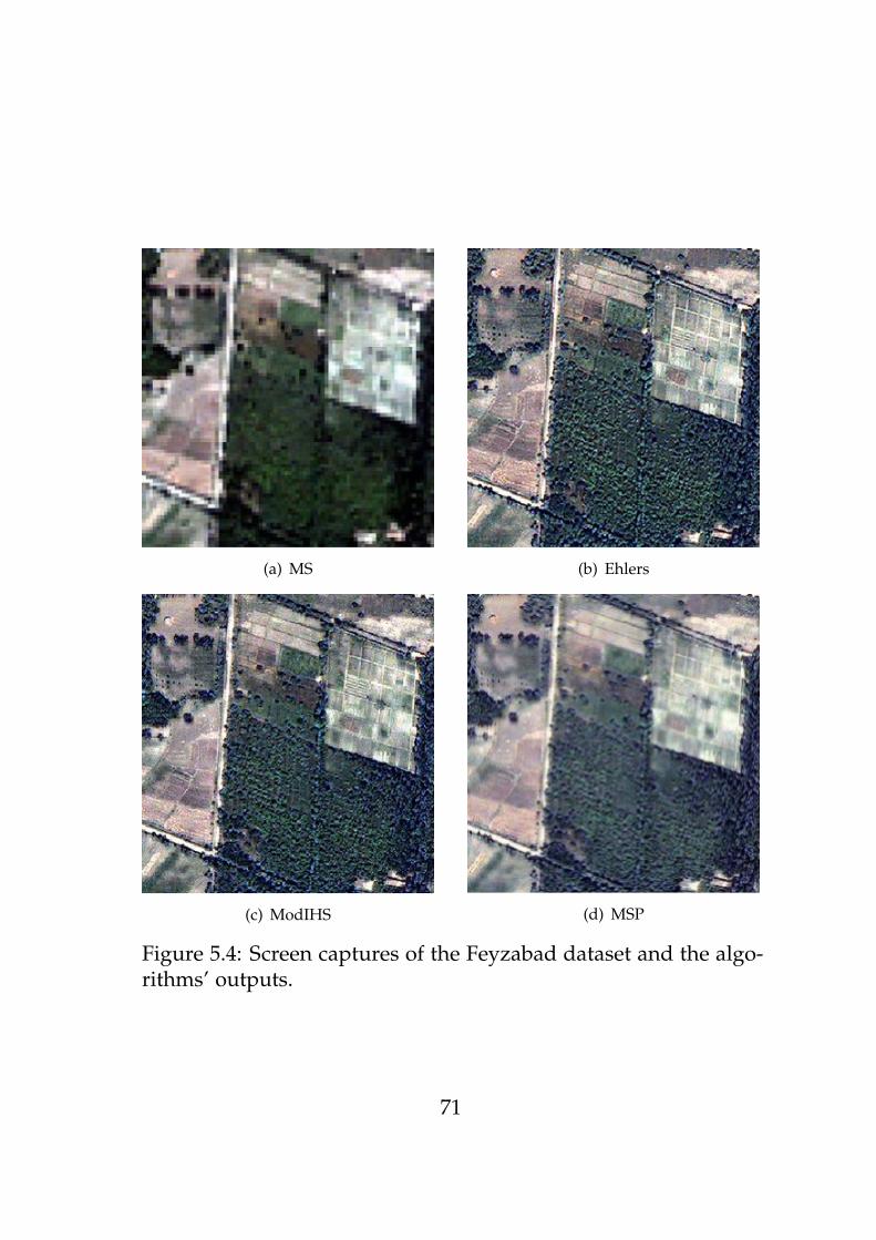
(a) MS (b) Ehlers

(c) ModIHS (d) MSP

Figure 5.4: Screen captures of the Feyzabad dataset and the algo-rithms’ outputs.

71

5.5 Quality Metrics

The preceding qualitative assessment gives a rough indication ofhow successfully an algorithm preserves the multispectral charac-teristics of a dataset while improving its spatial resolution. How-ever, we also provide objective measurements by means of thefollowing similarity metrics:

PD The Per-pixel Deviation is the difference of each component cof the pixels at coordinates i, j in the multispectral input B vs.those in the pan-sharpened output F after resampling to theoriginal resolution. It is normalized according to the imagedimension N ×M and number of components C. The bestvalue is zero. [112]

PD =

C

∑c=1

M

∑i=1

N

∑j=1

∣∣Bi,j,c − Fi,j,c∣∣

NMC(5.4)

RMSE Root Mean Square Error is simply the square-root of theMSE between the fused image and the original multispectralimage. Smaller values are better.

RMSEc =

√√√√√√M

∑i=1

N

∑j=1

(Bi,j,c − Fi,j,c

)2

NM(5.5)

CC Correlation Coefficient expresses the correlation between theoriginal and fused images and ranges from -1 to +1. Values

72

near 1.0 indicate the images are highly correlated and sim-ilar. [125] Let Fc denote the average intensity ∑i,j Fi,j,c/N ofeach pixels’ component c in F, and similarly Bc for B.

Corrc =

M

∑i=1

N

∑j=1

(Bi,j,c − Bc)(Fi,j,c − Fc)√√√√ M

∑i=1

N

∑j=1

(Bi,j,c − Bc)2

M

∑i=1

N

∑j=1

(Fi,j,c − Fc)2

(5.6)

ERGAS The relative dimensionless global error in fusion summa-rizes the errors in all bands. Smaller values indicate higherimage quality. The scaling factor h

l corresponds to the ratioof pixel sizes in the pan and MS imagery. [126]

ERGAS = 100hl

√1C

C

∑c=1

(RMSEc

Bc

)2

(5.7)

Q The Universal Image Quality Index incorporates loss of correla-tion, luminance distortion, and contrast distortion. It rangesbetween 0 and 1 and is maximized when the images areidentical. [127]

Qc =4BcFc ∑i,j (Bi,j,c − Bc)(Fi,j,c − Fc)

(B2 + F2)[∑i,j (Bi,j − Bc)2 + ∑i,j (Fi,j − Fc)2

] (5.8)

Q4 The ‘Quaternions Theory Based Quality Index’ is a generaliza-tion of the Q index to four bands via quaternions, computedon non-overlapping 32× 32 blocks. The best value is 1. [128]

73

Table 5.2: Per-band metrics for the Karlsruhe and Feyzabaddatasets. The best value of each metric is encircled.

Karlsruhe Feyzabad

CC Ehlers ModIHS MSP Ehlers ModIHS MSP

B 0.926 0.927 0.956 0.986 0.968 0.979G 0.956 0.956 0.982 0.993 0.978 0.991R 0.971 0.970 0.986 0.997 0.984 0.993

NIR 0.743 0.950 0.992 0.994 0.957 0.987mean 0.899 0.951 0.979 0.992 0.972 0.988

RMSE Ehlers ModIHS MSP Ehlers ModIHS MSP

B 0.330 19.58 13.69 0.713 9.55 5.899G 1.840 24.06 13.96 1.010 13.42 6.378R 3.001 23.55 14.66 1.155 14.29 7.035

NIR 0.631 60.13 22.46 1.197 23.30 9.493mean 1.451 31.83 16.19 1.019 15.14 7.201

Q Ehlers ModIHS MSP Ehlers ModIHS MSP

B 0.417 1.000 1.000 0.944 1.000 1.000G 0.554 0.999 1.000 0.961 1.000 1.000R 0.430 0.867 0.942 0.982 1.000 1.000

NIR 0.488 0.929 0.994 0.990 1.000 1.000mean 0.472 0.949 0.984 0.969 1.000 1.000

The values of the per-band metrics are given in Table 5.2. Asexpected, most outputs are highly correlated to the inputs. How-ever, the NIR band of the Ehlers result for the Karlsruhe datasetapparently includes some discrepancies, because its correlationcoefficient is only 0.7428. RMSE is higher for the IHS-based al-gorithms. Especially large differences in the ModIHS NIR bandare likely due to the original IHS strategy of obtaining the fourthband by substituting for another band and repeating the algorithm.Our approach avoids this issue by adding detail information to all

74

MS bands simultaneously. Although the resulting RMSE is stillhigher than the Ehlers output, the image quality is not necessarilyinferior [126]. For example, the underlying L2 norm unduly penal-izes outliers. By contrast, the Q index provides a more accurateindication of actual information loss [127]. According to this metric,the IHS-based approaches significantly outperform the Ehlers Fu-sion. As expected, our optimal weight estimation scheme improvesupon the fixed-weight ModIHS in all measurements. Let us nowexamine the global metrics across all bands, given in Table 5.3.The Ehlers Fusion results in the best ERGAS. However, this metric

Table 5.3: Global metrics for the Karlsruhe and Feyzabad datasets.The best value of each metric is encircled.

Karlsruhe Feyzabad

Metric Ehlers ModIHS MSP Ehlers ModIHS MSP

PD 0.025 15.908 7.722 0.015 7.838 2.817ERGAS 0.140 1.749 0.953 0.045 0.662 0.316

Q4 0.084 0.724 0.788 0.433 0.891 0.940

cannot rule out spectral distortion [125]. By contrast, the Q4 indexaccounts for differences in spectral angle by computing the actualmultivariate correlation coefficient [119]. Our method significantlyoutperforms the Ehlers Fusion in terms of this metric. Becausethe Ehlers algorithm’s Q results exceed the values of Q4, we caninfer that a spectral shift has occurred. In summary, the EhlersFusion yields better values of RMSE, PD and ERGAS, whereasour approach rates higher according to Q and Q4. This kind ofdiscrepancy has motivated the pessimistic conclusion that currentmetrics are not capable of reliably measuring image quality or evensimilarity [125]. However, we believe the simplistic RMSE, PD andERGAS metrics have less bearing on perceived quality than themore elaborate Universal Quality index and Q4.

75

5.6 Performance

In designing and implementing our approach, we emphasizedefficiency. To gain a first impression of the resulting performance,let us compare the run times for each of the three methods on aX5365 CPU (3.0 GHz, 32 GiB FB-DDR2 RAM), shown in Table 5.4.Our approach is about 40 times as fast as ModIHS despite doing

Table 5.4: Elapsed time [s] for the three methods and two datasets.

Algorithm Karlsruhe Feyzabad

Ehlers 1 235 31 721ModIHS 359 285

MSP 9 6

more work (computing the band weights). Because the algorithmsare very similar, the difference is largely due to implementationtechniques – vectorization, parallelization and optimizing the nu-merical calculations. The run time of the Ehlers algorithm is muchhigher still. It is unclear why the smaller 61 MPixel Feyzabadimage required 25 times as long as the 87 MPixel Karlsruhe dataset.Even disregarding this difference, our algorithm remains over 100times as fast. We have also measured the throughput of our algo-rithm on the more recent test system (c.f. Section 2.3), shown inTable 5.5. As with the Bilateral Filter, performance tends to increaseon larger images due to amortization of overhead. Our softwareoutperforms a similar algorithm’s Matlab implementation [119] bya factor of 1134.

76

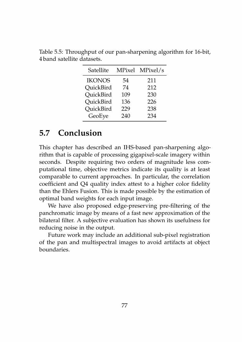
Table 5.5: Throughput of our pan-sharpening algorithm for 16-bit,4 band satellite datasets.

Satellite MPixel MPixel/s

IKONOS 54 211QuickBird 74 212QuickBird 109 230QuickBird 136 226QuickBird 229 238

GeoEye 240 234

5.7 Conclusion

This chapter has described an IHS-based pan-sharpening algo-rithm that is capable of processing gigapixel-scale imagery withinseconds. Despite requiring two orders of magnitude less com-putational time, objective metrics indicate its quality is at leastcomparable to current approaches. In particular, the correlationcoefficient and Q4 quality index attest to a higher color fidelitythan the Ehlers Fusion. This is made possible by the estimation ofoptimal band weights for each input image.

We have also proposed edge-preserving pre-filtering of thepanchromatic image by means of a fast new approximation of thebilateral filter. A subjective evaluation has shown its usefulness forreducing noise in the output.

Future work may include an additional sub-pixel registrationof the pan and multispectral images to avoid artifacts at objectboundaries.

77

Chapter 6

Image Segmentation

The next pipeline stage is responsible for automatically partitioningimages into regions (‘segmentation’). This chapter introduces aMinimum Spanning Tree-based algorithm with a novel graph-cutting heuristic, the usefulness of which is demonstrated bypromising results obtained on standard images. In contrast todata-parallel schemes that divide images into independently pro-cessed tiles, the algorithm is designed to allow parallelizationwithout truncating objects at tile boundaries. A fast parallel imple-mentation for shared-memory machines is shown to significantlyoutperform existing algorithms. It utilizes a new microarchitecture-aware single-pass sort algorithm, presented in Appendix A, that islikely to be of independent interest.

An initial version of this chapter appeared in the proceedings ofthe 13th International Conference on Computer Analysis of Imagesand Patterns [129].

6.1 Introduction and Related Work

Segmentation is an important early stage of some image processingpipelines, e.g. object-based change detection. The final results ofsuch applications are often strongly dependent on the quality ofthe initial segmentation. Because subsequent processing steps canuse higher-level region information instead of having to examine

79

all pixels, the segmentation may also be the limiting factor in termsof performance. Many algorithms have been proposed, but goodquality results often come at the price of high computational cost.

One extreme example of this is a multi-scale watershed ap-proach (MSHLK) [130]. Repeated applications of anisotropic diffu-sion smooth the image and reduce the tendency of the watershedtransform to return excessive numbers of segments (oversegmenta-tion). The resulting subjective quality is very good, but its process-ing speed (1 kPixel/s) is unacceptably low.

An alternative approach uses the Mean-Shift (MS) [131] proce-dure to locate clusters within a higher-dimensional representationof the image. This is guaranteed to converge on the densest regionsin this space and yields good results in practice, but the processingrate (100 kPixel/s) is still inadequate.

In previous work, we have shown that Maximally Stable Ex-tremal Regions (MSER) [132] can be applied towards segmentationof gradient images. Although more efficient (2 MPixel/s), thisscheme only detects high-contrast segments and does not providefull coverage of the image. It also seems ill-suited for paralleliza-tion because the criterion for ‘stable’ depends on a global orderingof pixels.

Graph-based segmentation (GBS) [133] increases the amount ofdata to be handled (multiple graph edges per pixel) but has severalattractive properties. Viewing pixels as nodes of a graph allowsthe reduction of segmentation to cutting a Minimum SpanningTree (MST). Defining edge weights as some function of the pixels’per-band intensity differences enables the use of color informationwithout having to compute image gradients1. Finally, an MST canbe assembled from partial sub-trees, which provides the possibilityof parallelization. In Section 6.2, we develop a new online graph-cutting heuristic for MST-based segmentation. Section 6.3 showsthe promising results obtained on well-known images. Section 6.4

1A measure of the change in intensity for each pixel, e.g. by computing differencesto neighboring pixels.

80

introduces ‘PHMSF’ (Parallel Heuristic for Minimum SpanningForests) , which we believe to be the first non-trivially-parallel seg-mentation algorithm. Perhaps most importantly, Section 6.6 showsit to significantly outperform existing segmentation techniques.

6.2 Algorithm

Segmentation algorithms require (often application-dependent)definitions of ‘image region’. We believe ‘homogeneity’ and highcontrast to surrounding pixels are reasonable criteria [134]. Ho-mogeneity can be computed as distances between (vector-valued)pixels; we find the L2 norm to yield better results than L1 orpseudo-norms. Prior work [133] has advocated separate segmenta-tion of the R/G/B component images and intersecting the results.Because object edges are not always visible in all multi-spectralbands [135], it is safer (and certainly faster) to segment once usingall bands. Recalling the graph segmentation framework, the abovehomogeneity measure defines the weight of edges. It remains tobe seen how an online graph-cutting heuristic should partition theMST depending on edge weight. A mere threshold is insufficientbecause it fails to account for noise or the overall homogeneity of aregion. One possible solution [133] involves an adaptive thresholdthat is incremented by a linearly decreasing function of the regionsize2. The function’s slope is a user-defined parameter that must bedetermined by experimentation because it has no physical expla-nation. This scheme also underestimates a region’s homogeneityby defining it as the maximum weight in its MST, thus tendingtowards oversegmentation. We suggest the adoption of an ideafrom Canny’s detector for image edges [136]. In the context of com-putational edge detection, pixels with large gradient magnitudesare likely to correspond to edges within the image, but there is no

2This unduly penalizes the growth of large segments; we saw slightly better resultswhen dividing by the logarithm of the region size.

81

single level at which this ceases to be the case. Applying a relativelystrict threshold finds safe candidates, which can be augmented bynearby pixels that lie above a second, more generous limit. Return-ing to segmentation terminology, regions connected by low-weightgraph edges represent likely candidates that can subsequently beexpanded by following adjoining graph edges with somewhathigher weights. Figure 6.1 illustrates how a region is formed byexpanding the initial candidate. To avoid potentially unbounded

Figure 6.1: A region is obtained by expanding an initial candidateformed from homogeneous pixels.

growth, we institute a ‘credit’ limit on the sum of edge weightsthat may be added to a candidate region. The motivating principle– how much water can be filled into a basin without overflowing –is shown in Figure 6.2. Because a circle is the most compact two-dimensional shape [137], its circumference

√4π × regionSize

constitutes a lower bound on the perimeter (minPerimeter) ofa region whose area is regionSize pixels. Let us also assumeadditive white Gaussian noise with variance σ2

n, for which severalestimators have been proposed [138, 139]. With an eye towardsthe Gaussian cumulative distribution function, we choose 2σn asan arbitrary cutoff point. It is unlikely for any larger intensitydifferences to arise from noise. We therefore define minContrastas the smallest edge weight along the border of any ‘interesting’region minus 2σn. Putting both these pieces together, the functionComputeCredit := minContrast × minPerimeter estimatesthe total weight of edges whose endpoint pixels can be added

82

Figure 6.2: Motivation for the credit computation. The gray areadenotes a region being filled with water. Spilling beyond its boundscan only occur if the total volume exceeds a function of the perime-ter and the minimum wall height (the red lines of varying heightsuggest boundary edges and their weights).

to a region without inadvertently expanding beyond its bounds.This property is important because subsequent region merge deci-sions can be based upon region features (discussed in Section 6.5),whereas splitting requires re-examination of the pixels or edges.However, the resulting regions are not necessarily too fine becausepixels connected by low-weight edges are always merged. Wehave therefore averted global under- and oversegmentation of theimage while using only local information. The algorithm firstforms candidate regions by merging the endpoints of low-weightedges, computes their credit, and then calls a simple heuristic (Al-gorithm 6.1) in increasing order of the remaining edges’ weights.

83

Algorithm 6.1: EdgeHeuristic(edge)1 region1, region2 := Find(edge.endpoints);2 if region1 6= region2 then3 credit := min region1.credit, region2.credit;4 if credit > edge.weight then5 survivor := Union(region1, region2);6 survivor.credit := credit− edge.weight;7 end8 end

Implementation Details

We represent edges as 30-bit integers indicating the index of theiroriginating node together with a 2-bit encoding of their four possi-ble directions3.

Nodes (pixels) are organized into ‘disjoint sets’ (regions) bymeans of the Union-Find (UF) data structure [140]. Each node is as-sociated with a 32-bit value that typically points to its parent node.The root of each subtree (i.e. region) is termed the ‘[canonical]representative’ and holds the index of the corresponding regiondata structure, which stores credit and size in 32-bit integers.We differentiate parents and representatives by means of their signbit. This avoids the need for auxiliary storage during the initialregion merging, because credit is not yet needed and the rep-resentative stores the (negated) size. Find traverses the parentlinks and returns the representatives of the regions adjoining thegiven edge. To speed up these relatively expensive (due to theirpoor locality) searches, we halve the subsequent path length inevery iteration by reassigning nodes’ parents to their grandparents.Union merges two regions; choosing the larger one as the parentalso serves to decrease path lengths [140]. We introduce an addi-tional optimization that avoids needing to initialize the parent array

3Each node has eastern, southern, southwestern and southeastern connections toits neighbors, thus yielding an eight-connected grid graph.

84

and halves the number of allocated region structures. Because Win-dows’ VirtualAlloc returns zeroed memory, we consider 0 tobe a valid region index. Recall that nonpositive 32-bit indices areinterpreted as representatives. We allocate enough virtual addressspace to treat indices as unsigned 32-bit offsets and then map asingle (read-only) page of zeroed memory at the address of region0. When a node is first merged, its size therefore appears to bezero, thus causing it to be linked to the (larger) parent. We onlyneed to allocate a region structure when the parent also reports asize of zero. Physical memory for subsequent region structures iscommitted as needed.

6.3 Results

To demonstrate the usefulness of the new segmentation results, wecompare them to the outputs of existing algorithms on standardimages [141], the results of which are shown in Figures 6.3 and6.4. MSHLK [130] is known for high-quality results and providesexcellent smoothing of the walls (b) but merges the eaves into thesky segment. We also call attention to the oversegmentation ofthe second image and shock effects [142] in the background (b).MS [131] is more successful at merging the individual objects (c)but also splits some of them (e.g. below the P); spurious segmentsnear edges (c) are its only visible flaws. As with MSHLK, seg-ment borders are delineated by black pixels. MSER [132] producesmostly adequate label images, though the wall is not considered tobe a stable region (d); the effects of the gradient filter are clearlyvisible (d). GBS [133] is satisfactory but results in undersegmenta-tion near the roof lines and oversegmentation of the sky and wall(e). It also merges different-colored objects (e) but fails to return auniform background. Our new PHMSF algorithm provides resultscomparable to MSHLK and MS and requires only 1/4 000 and 1/50the computation time, respectively (c.f. Section 6.6). The black pix-els (f) indicate surface irregularities that resulted in regions smaller

85

(a) Image (b) MSHLK

(c) MS (d) MSER

(e) GBS (f) PHMSF

Figure 6.3: Segmentation results of the new PHMSF algorithm andothers on USC SIPI [141] image 4.1.05 (‘House’).

86

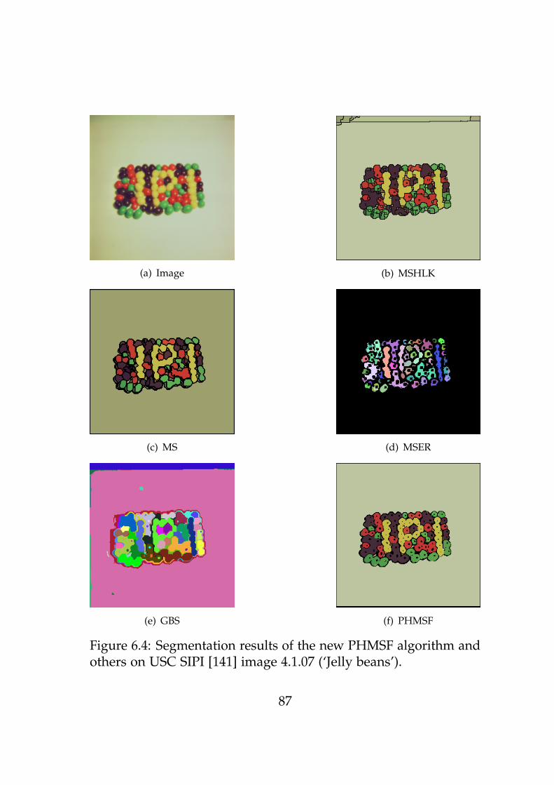
(a) Image (b) MSHLK

(c) MS (d) MSER

(e) GBS (f) PHMSF

Figure 6.4: Segmentation results of the new PHMSF algorithm andothers on USC SIPI [141] image 4.1.07 (‘Jelly beans’).

87

than the minimum size. The segmentation in (f) is quite accurate,correctly separating different-colored objects without introducingspurious boundaries.

6.4 Parallel Algorithm

Despite the efficiency of the new segmentation algorithm, a highly-tuned sequential implementation is still far slower than the collec-tion rates of commercial imaging satellites (e.g. IKONOS with up to90 km2/s [110]). Because significant reductions of the algorithm’sconstant factors or major increases in single-core CPU performance(c.f. Section 2.4) appear unlikely, our self-set performance goal of10 MPixel/s requires parallelization. However, ‘embarrassinglyparallel’ schemes that simply split the input into independent tilesare not acceptable because they do not correctly handle objectsstraddling a border. Nor are overlapping tiles sufficient becausethere is no upper bound on the size of objects of interest (e.g. riversor roads). Our first attempt at parallelization addressed the MSTcomputation. The recently introduced Filter-Kruskal scheme [143]combines ideas from Quicksort and Kruskal’s algorithm and dis-cards non-MST edges without having to sort them. This ‘filter’operation, partitioning and sorting can all be parallelized. How-ever, the total speedup on a quad-core system is only 1.5 – chieflydue to the sequential portion of the algorithm, but also because oureight-connected grid graphs are too sparse to derive much benefitfrom discarding edges. Our second approach (Algorithm 6.2) isdesigned to allow independent processing of image tiles, but stillensures consistent results irrespective4 of the number of processorsP. The key observation is that Kruskal’s MST algorithm can run ina data-parallel fashion until encountering an edge that crosses a tile

4We ignore the effects of ‘unstable’ parallel sorting. The relative order of items withthe same key depends on the number of processors and the arbitrary manner in whichthe grid graph is constructed. However, neither appears to have a relevant influence onthe results.

88

Algorithm 6.2: Parallel Segmentation1 parallel foreach tile do2 sort edges in ascending order of weight;3 immediately merge regions connected by edges of weight

< minWeight;4

5 foreach borderEdge do // connect and mark cross-borderregions

6 region1, region2 := Find(borderEdge.endpoints);7 survivor := Union(region1, region2);8 Mark(survivor);9 tile.regions := tile.regions∪ survivor;

10 end11 parallel foreach tile do12 foreach r ∈ tile.regions do

r.credit := ComputeCredit(r.size); // see Section 6.213

14 parallel foreach tile do15 foreach edge in ascending order of weight do16 region1, region2 := Find(edge.endpoints);17 if edge crosses border then

Mark(region1), Mark(region2);18 else if IsMarked(region1) or IsMarked(region2)

then tile.delayQ.Push (edge) ;19 else EdgeHeuristic(edge); // see Section 6.220 end21

22 foreach tile do23 foreach edge ∈ tile.delayQ do EdgeHeuristic(edge);24 end

89

Figure 6.5: Top view of a graph representing two square tiles withinthe input image. Nodes are located at the intersections of the dottedlines, and non-discarded MST edges are rendered as colored lines.Processors can run Kruskal’s algorithm independently on their tilesuntil reaching one of the red edges (i.e. those directly or indirectlyconnected to a cross-tile edge).

border (c.f. Figure 6.5). From then on, MST components using suchedges and in turn their incident edges must be ‘delayed’ until thepartial MSTs of both tiles are available. This can be accomplished byadding edges to per-tile queues that are processed in a subsequentsequential phase5. We also Mark any regions reachable via delayededges by setting the most-significant bit of their size, which canbe queried by IsMarked. It remains to be seen how many edgesare delayed – a long cross-border region of homogeneous pixelscould affect a large proportion of a tile. However, high-weightedges at the boundary of such regions often serve as a ‘firewall’ be-cause they can be discarded without affecting neighboring regions.Only about 5% of edges are delayed in practice, making Amdahl’s

5This would be parallelizable if edges indicate which border they cross, but ourimplementation cannot spare any space within the 32-bit representation.

90

argument less of a factor than real-world limits on memory band-width and P. To avoid scheduling and locality issues, the manuallypartitioned loops reside in a single OpenMP parallel region (c.f.Section 2.4). A novel variant of counting sort uses paged virtualmemory to simulate bins of unlimited size and thus dispenses witha separate counting phase. An explicit buffering technique furtherincreases performance by enabling write-combining without cachepollution. Details are given in Appendix A.2.

6.5 Region Features

The algorithm also computes region features. However, it would bewasteful to allocate records for the numerous small regions that areoften ignored by applications anyway. We therefore only considerregions whose size lies within a user-defined interval [min, max].This entails relabeling the per-tile regions and replacing themwith a new set of contiguous indices, which is accomplished byAlgorithm 6.3. Its separate and very efficient count phase seemspreferable to updating the per-tile region count when cross-bordermerges are performed by our parallel Kruskal algorithm. One ofthe typical outputs of a segmentation algorithm is a label image –the value of a pixel indicates the region to which it belongs. Wetherefore ‘collapse’ the array of Union-Find parents such that eachnode points directly to its representative once all regions have beenre-labeled.

Let us now examine the data structure referenced by the newindices. Maintaining a list of member pixels for each region wouldbe costly in terms of time and space. We instead iterate over theimage pixels and ascribe their properties to the correspondingregion. This improves locality when the region features requireless storage than the pixels themselves6. Updating the features

6Our region descriptors currently occupy 64 bytes, whereas a pixel comprises4 components of 2-byte numbers, and regions usually encompass more than 8 pixels.

91

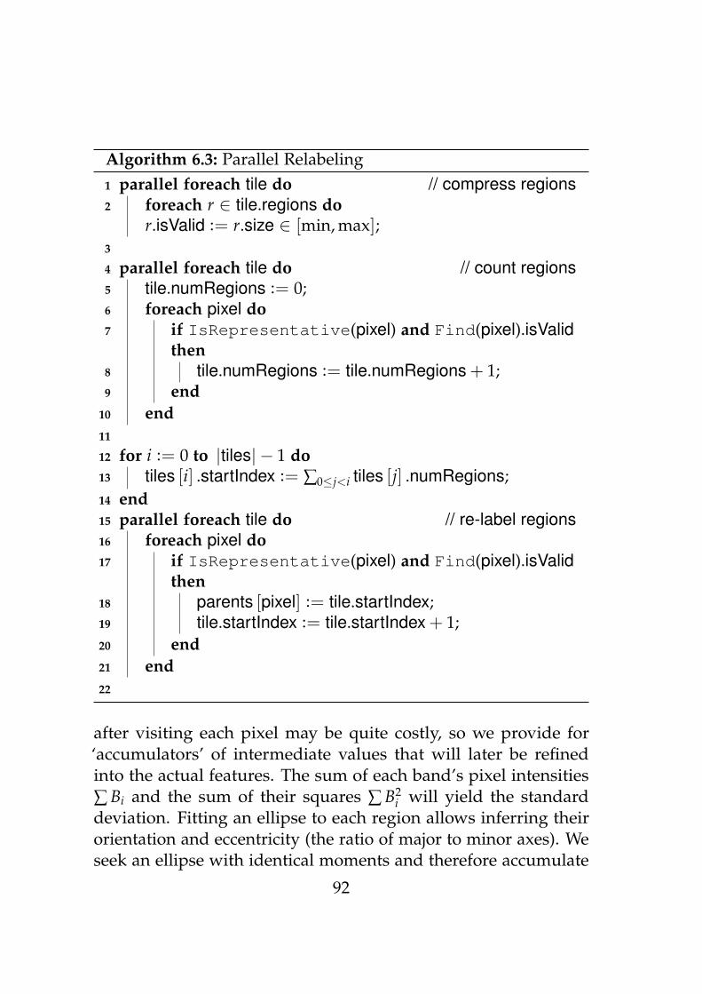
Algorithm 6.3: Parallel Relabeling1 parallel foreach tile do // compress regions2 foreach r ∈ tile.regions do

r.isValid := r.size ∈ [min, max];3

4 parallel foreach tile do // count regions5 tile.numRegions := 0;6 foreach pixel do7 if IsRepresentative(pixel) and Find(pixel).isValid

then8 tile.numRegions := tile.numRegions + 1;9 end

10 end11

12 for i := 0 to |tiles| − 1 do13 tiles [i] .startIndex := ∑0≤j<i tiles [j] .numRegions;14 end15 parallel foreach tile do // re-label regions16 foreach pixel do17 if IsRepresentative(pixel) and Find(pixel).isValid

then18 parents [pixel] := tile.startIndex;19 tile.startIndex := tile.startIndex + 1;20 end21 end22

after visiting each pixel may be quite costly, so we provide for‘accumulators’ of intermediate values that will later be refinedinto the actual features. The sum of each band’s pixel intensities∑ Bi and the sum of their squares ∑ B2

i will yield the standarddeviation. Fitting an ellipse to each region allows inferring theirorientation and eccentricity (the ratio of major to minor axes). Weseek an ellipse with identical moments and therefore accumulate

92

mp,q = ∑ XpYq (p, q ∈ N0, p + q ≤ 2) for each of the region’spixels with coordinates (X, Y). [144] These values are stored as64-bit floating point numbers to mitigate precision issues whilestill enabling vectorization via SSE2 instructions. It is also possibleto estimate the region perimeter from a single sequential scan ofits pixels. To that end, we count numEqual, the number of edgeswhose endpoints have the same label. The central pixel is copiedinto each lane of a vector and compared to a vector comprising thefour surrounding pixels. This results in 32-bit masks with all bitsset if the corresponding value was equal. After packing the masksinto 16-bit representations, we compute their byte-wise horizontalsum by means of the PSADBW7 SSE2 instruction. A final set ofaccumulators involve the maximum X and Y coordinates, whichwill be used to construct the axis-aligned bounding box (AABB).As with the parent indices, we can avoid explicit initialization ofthe accumulators if their initial values are zero. This is the case foraccumulators representing counters or maximum values. However,AABBs also require the minimum coordinates. To avoid a specialcase for their initial values, we instead track the maximum additivecomplement of the coordinates. Their values can be represented asfloats without loss, so we are able to update the four maxima witha single SIMD MAXPS8 instruction.

Each CPU core is assigned a strip of the image, for which itupdates a set of accumulators. Pairs of accumulator arrays aresuccessively reduced to a single global array by taking the max-imum of the coordinates, and adding all other values. We thencompute each region’s features from its accumulator. Let n = m0,0

denote the region size. The i-th band average µi is ∑ Bi/n, with

standard deviation ∑ B2i −nµ2

in . The centroid, i.e. center of mass, is

(m1,0

n , m0,1n ). For the ellipse fit, we require the normalized sam-

ple central moments µ1,1 =m1,1

n − m1,0m0,1, µ2,0 =m2,0

n − m1,0m1,0

and µ0,2 =m0,2

n − m0,1m0,1. The orientation is then given by7Packed Sum of Absolute Differences (Byte to Word).8MAXimum Packed Single-precision value.

93

12 arctan( 2µ1,1

µ2,0−µ0,2) [145]. To form an equal-area ellipse, we divide

the moments by µ2,0µ0,2 − µ1,1µ1,1 [146, p. 283]. Solving for the

major and minor axes yields√

8a+c∓d , with d =

√(a− c)2 + 4b2

[147]. The AABB is constructed from the X, Y maxima and thedifference between the largest possible value and the accumulatedmaxima of the coordinates’ complements. Finally, a measure of theregion’s compactness is useful for differentiating ragged naturalstructures from more regular man-made objects. The isoperimetricquotient 4πn

L2 is frequently used in this context [148]. Its maximumof 1.0 is reached in the case of a circle. To estimate the perimeterL, let us review the properties of an 8-connected grid graph. Aregion touches 8n edges, and each boundary pixel accounts for 1to 7 of them. We assume an average of two such edges for everypixel-width segment along the region’s boundary. numEqual isobtained by dividing the PSADBW accumulator by 510, because itis the horizontal sum of pairs of 8-bit mask halves, each of whichare 0 or 255. Therefore, L ≈ 8n−numEqual

2 .

6.6 Performance

We first examine the complexity of the proposed algorithm. Count-ing sort is O(n). Region merges via Union-Find are effectivelyO(1) for all practical input sizes9 [150]. All other operations arealso constant-time and reside in loops with iteration counts inO(n), so the complexity is (quasi-)linear in the input size. Becausethis also applies to the MSER and GBS algorithms, we must com-pare their implementations. Table 6.1 lists the performance10 ofeach algorithm for a representative 8.19 MPixel subset of a 16-bit,

9We view the inverse Ackermann function as a constant ≤ 5 for n < 1080. Notethat an attempt at replacing Union-Find with a ‘true linear algorithm’ [149] introducesa constant factor of 8.

10Measured on a X5365 CPU (3.0 GHz, 32 GiB FB-DDR2 RAM) running WindowsXP x64. Our implementation is compiled with ICC 11.0.066 /Ox /Og /Ob2 /Oi /Ot/fp:fast /GR- /Qopenmp /Qftz /QxSSSE3.

94

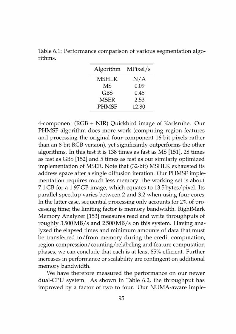
Table 6.1: Performance comparison of various segmentation algo-rithms.

Algorithm MPixel/s

MSHLK N/AMS 0.09GBS 0.45

MSER 2.53PHMSF 12.80

4-component (RGB + NIR) Quickbird image of Karlsruhe. OurPHMSF algorithm does more work (computing region featuresand processing the original four-component 16-bit pixels ratherthan an 8-bit RGB version), yet significantly outperforms the otheralgorithms. In this test it is 138 times as fast as MS [151], 28 timesas fast as GBS [152] and 5 times as fast as our similarly optimizedimplementation of MSER. Note that (32-bit) MSHLK exhausted itsaddress space after a single diffusion iteration. Our PHMSF imple-mentation requires much less memory: the working set is about7.1 GB for a 1.97 GB image, which equates to 13.5 bytes/pixel. Itsparallel speedup varies between 2 and 3.2 when using four cores.In the latter case, sequential processing only accounts for 2% of pro-cessing time; the limiting factor is memory bandwidth. RightMarkMemory Analyzer [153] measures read and write throughputs ofroughly 3 500 MB/s and 2 500 MB/s on this system. Having ana-lyzed the elapsed times and minimum amounts of data that mustbe transferred to/from memory during the credit computation,region compression/counting/relabeling and feature computationphases, we can conclude that each is at least 85% efficient. Furtherincreases in performance or scalability are contingent on additionalmemory bandwidth.

We have therefore measured the performance on our newerdual-CPU system. As shown in Table 6.2, the throughput hasimproved by a factor of two to four. Our NUMA-aware imple-

95

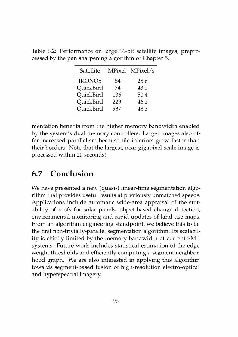
Table 6.2: Performance on large 16-bit satellite images, prepro-cessed by the pan sharpening algorithm of Chapter 5.

Satellite MPixel MPixel/s

IKONOS 54 28.6QuickBird 74 43.2QuickBird 136 50.4QuickBird 229 46.2QuickBird 937 48.3

mentation benefits from the higher memory bandwidth enabledby the system’s dual memory controllers. Larger images also of-fer increased parallelism because tile interiors grow faster thantheir borders. Note that the largest, near gigapixel-scale image isprocessed within 20 seconds!

6.7 Conclusion

We have presented a new (quasi-) linear-time segmentation algo-rithm that provides useful results at previously unmatched speeds.Applications include automatic wide-area appraisal of the suit-ability of roofs for solar panels, object-based change detection,environmental monitoring and rapid updates of land-use maps.From an algorithm engineering standpoint, we believe this to bethe first non-trivially-parallel segmentation algorithm. Its scalabil-ity is chiefly limited by the memory bandwidth of current SMPsystems. Future work includes statistical estimation of the edgeweight thresholds and efficiently computing a segment neighbor-hood graph. We are also interested in applying this algorithmtowards segment-based fusion of high-resolution electro-opticaland hyperspectral imagery.

96

Chapter 7

Antialiased Line Rasterization

This chapter presents an efficient, high-quality software line ras-terizer for annotating very large images with segment contours.Although many fast line drawing algorithms are known, mostproduce thin and ‘jagged’ lines due to aliasing. Wu’s algorithmincludes a crude approximation of antialiasing, which still includesnoticeable step edges. Even hardware multisampling cannot en-tirely eliminate aliasing. Instead, the proper solution is to removehigh-frequency components by pre-filtering the lines. We improveupon previous ad-hoc filters by deriving the optimal (in the senseof minimizing aliasing) cubic polynomial filter. When combinedwith our new, optimized variant of the Gupta-Sproull line draw-ing algorithm, this outperforms Wu’s fast approximation whiledelivering much higher-quality results.

A preliminary version of this chapter appeared in the proceed-ings of the Fourth Pacific-Rim Symposium on Image and VideoTechnology [154].

7.1 Introduction and Related Work

Scan-converting line segments for raster-based displays or imagesis a basic building block of many computer graphics tasks. Oneapplication involves plotting the contours of image segments toaid human recognition of man-made objects. Current CPUs can

97

easily annotate high-definition video frames, but the timely pro-cessing of gigapixel-scale imagery remains an interesting challenge.GPUs cannot yet handle such large amounts of data due to texturedimension and memory size1. We therefore consider software linedrawing approaches from the literature.

Fast Line Drawing Algorithms

Bresenham’s Midpoint algorithm [155] is the foundation of mostsubsequent line-drawing schemes. The Digital Differential Ana-lyzer is similar, but avoids conditional branches, which are expen-sive given the deep pipelines of modern CPUs. Several furtherattempts have been made to speed up the underlying algorithm.Gardner [156] and Boyer/Bourdin [157] take advantage of symme-try by simultaneously drawing from both ends of the line segment.Although the iteration count is halved, this leads to more complexmemory access patterns, which may be problematic for hardwareprefetchers. Rokne [158] additionally considers two pixels at atime, again halving the iteration count at the expense of manymispredicted conditional branches. Bresenham’s run-length slicealgorithm [159] avoids redundant per-pixel decisions by comput-ing the length of horizontal pixel runs. However, special cases forevery possible run-length [160] would greatly increase the codesize. These optimizations appear to be intended for long lines, buta survey of applications [161] has found that 87% of line segmentsare less than 17 pixels long. This suggests favoring simple mainloops over complex strategies for reducing the iteration counts.With regard to output quality, all of the above algorithms producethin lines with ‘jaggies’ (a stairstep effect due to aliasing).

1The 4 GiB memory limit on current GPUs is due to DRAM density and interfacewidth. It can be doubled by means of the recent GDDR5 standard’s clamshell mode [10],but still falls far short of the 192 GiB available to commodity workstations.

98

Antialiasing

Antialiasing is desirable because it removes spurious informationand enables subpixel accuracy localization by the human visualsystem [162]. The cause of aliasing is shown by the sampling the-orem, which indicates a function may be faithfully reconstructedfrom samples spaced 1

2 fNapart if it has no energy in frequencies

≥ fN. Otherwise, the higher frequencies are aliased to lower fre-quencies. There are three ways to mitigate this [163]. Pre-filteringthe image prior to reconstruction can reduce the effects of aliasing,at the cost of losing detail and sharpness. However, we are notwilling to presuppose specific reconstruction filters [164] for themonitor/printer/eye. Sampling at a higher resolution is exem-plified by hardware multisampling, but has practical limits andcannot entirely avoid aliasing. Instead, pre-filtering the continuousobjects prior to sampling is the most promising route.

Wu’s antialiasing technique [165] involves shading pairs of pix-els straddling a line in proportion to their vertical distance from theline. This corresponds to a box filter – a crude approximation of therequisite low-pass filter that allows some high frequencies to passthrough [166]. However, the algorithm has found widespread usedue to its simplicity and speed, and efficient implementations [167]using fixed-point arithmetic are available.

Gupta and Sproull (GS) [168] propose low-pass filtering witha conical point-spread function (PSF). Being radially symmetric,its convolution with a line only depends on the perpendiculardistance to the line. The distance is incrementally computed by analgorithm similar to Bresenham’s, and the result of the convolutionretrieved from a small lookup table. This framework is usefulbecause it allows antialiasing with any radially symmetric PSFat little additional cost. However, it is unclear why a conicalPSF was chosen – perhaps the numerical integration of a morecomplex function was too expensive at the time. The use of ad-hocPSFs is also exemplified by more recent GPU-based prefiltering

99

approaches [169, 170, 171] using conical, Gaussian and exponentialPSFs. We point out their weaknesses and derive an optimal PSF(in the sense of minimizing aliasing) in Section 7.4.

Chen [172] suggests a variant of the GS algorithm that supportsfloating-point endpoint coordinates, which do not arise in ourapplication, and slightly accelerates the main loop by computingperpendicular distances via trigonometry.

We describe further major optimizations that result in a 24.6-fold speedup in Section 7.2. Our implementation therefore out-performs Wu’s fast approximation according to the measurementsin Section 7.3. However, the new PSF yields much higher-qualitylines, as shown by Section 7.5.

7.2 Algorithm

We begin with Chen’s [172][p. 23] improved version of GS (Algo-rithm 7.1). The underlying assumption that lines reside in thefirst octant can be avoided by transposing/mirroring. To avoidredundant pointer arithmetic, we combine the x, y arguments ofIntensityPixel (defined in Section 7.4) into a current-positionpointer; incrementing y is accomplished by adding ‘pitch’ (the sizeof a scanline). Expensive bounds checks for every pixel are avoidedby special-casing horizontal and vertical lines and otherwise disal-lowing points lying on the image border. Our main improvementis avoiding the mispredicted conditional branch in line 10 by usinga bitmask derived from the sign of the discriminator d to selectbetween possible summands for d and D (the signed perpendiculardistance from the line, c.f. Algorithm 7.1). In fact, the commonsubexpressions allow unconditionally adding the first term 2∆yto d (∈ Z) and then subtracting (2∆x) & mask. Doing the samefor D is safe because the IEEE-754 floating-point representationof 0.0 is all zeros. Negating the discriminator d allows obtainingthe mask via signed right shift, which replicates the sign bit. We

100

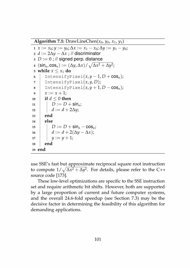
Algorithm 7.1: DrawLineChen(x0, y0, x1, y1)1 x := x0; y := y0; ∆x := x1− x0; ∆y := y1− y0;2 d := 2∆y− ∆x ; // discriminator3 D := 0 ; // signed perp. distance4 (sinα, cosα) := (∆y, ∆x)/

√∆x2 + ∆y2;

5 while x ≤ x1 do6 IntensifyPixel(x, y− 1, D + cosα);7 IntensifyPixel(x, y, D);8 IntensifyPixel(x, y + 1, D− cosα);9 x := x + 1;

10 if d ≤ 0 then11 D := D + sinα;12 d := d + 2∆y;13 end14 else15 D := D + sinα − cosα;16 d := d + 2(∆y− ∆x);17 y := y + 1;18 end19 end

use SSE’s fast but approximate reciprocal square root instructionto compute 1/

√∆x2 + ∆y2. For details, please refer to the C++

source code [173].These low-level optimizations are specific to the SSE instruction

set and require arithmetic bit shifts. However, both are supportedby a large proportion of current and future computer systems,and the overall 24.6-fold speedup (see Section 7.3) may be thedecisive factor in determining the feasibility of this algorithm fordemanding applications.

101

7.3 Performance

The complexities of the GS variants and Wu algorithm are linear,because each coordinate on the major axis is visited exactly onceand all operations are O(1). However, their constant factors varyaccording to the number of pixels shaded and the efficiency ofthe loop bodies. These effects are best observed by measuring2

the time required to draw many long lines, thus de-emphasizingfunction call and setup overhead. Table 7.1 shows the resulting‘fillrates’ when drawing 64 Ki parallel lines (sorted by increasing ycoordinate) with slope ≈ −1/8 and length ≈ 8 Ki. Note the large

Table 7.1: Performance (peak fillrate) of various line rasterizers.

Algorithm MPixel/s

Original GS (Table) 107Parallel GS (Table) 847

Wu (2 pixels) 1898Optimized GS (Table) 2387

Optimized GS (Polynomial) 2634

ratio of 24.6 between the ‘original’ (Chen’s improved variant of theGS algorithm) and our final optimized version. Shared-memoryparallelization achieves a nearly linear speedup for all algorithms(processors can draw lines independently unless they write to thesame cache line, in which case hardware cache coherency incurssome overhead). A careful implementation [167] of Wu’s simpleline drawing algorithm is 2.2 times as fast, because it only requiresa few fixed-point operations per loop and shades two instead ofthree pixels. However, our optimized variant of GS is even faster,outperforming the original version by a factor of 2.8 and Wu’s

2Test platform: dual W5580 CPUs (3.2 GHz, 48 GiB RAM) run-ning Windows XP x64. Compiler: ICC 11.1.082 /Ox /Og /Ob2 /Oi/Ot /Qipo /GA /MD /GS- /fp:fast=2 /GR- /Qopenmp /QxSSE4.1/Quse-intel-optimized-headers.

102

algorithm by 1.3. Its performance is on par with the fillrate of amid-range GPU (NVIDIA GeForce 9600 GT) [174].

Table lookup versus arithmetic

Interestingly, the final version of our implementation is an addi-tional 10% faster due to SIMD-based evaluation of the cubic poly-nomial. This result deserves closer analysis, because conventionalwisdom suggests that (small) lookup tables outperform arithmetic.The dependency chain of a Horner scheme ((h3x + h2)x + h1)x + h0

involves three additions and multiplications. These instructionshave had fairly consistent latencies of 3 or 4 cycles in the x86 mi-croarchitectures of the past 10 years [56], for a total of ≈ 24. Thisis in contrast to a table lookup that only requires a multiplica-tion, rounding/truncation and load. Whereas memory latencycontinues to increase with respect to the CPU clock [42], a small,frequently accessed table can be assumed to reside in the L1 cache.The total latency is therefore on the order of ≈ 12 cycles. A firstattempt to close this gap might involve vector instructions to speedup the computation of < (h0, h1, h2, h3)T, (1, x, x2, x3)T >. However,the high latency of the SSE4.1 instruction set’s horizontal dot prod-uct erodes any benefits. To realize the full potential of SIMD, theapplication must compute several independent results in parallel.When amortized over the four operations per SSE instruction, eachevaluation of the polynomial only requires 6 cycles. In this case,we are limited to the three pixels straddling the line, because thecomputation of subsequent pixels requires different operands. Ingeneral, we recommend replacing table lookups with (e.g. cubic)interpolation polynomials whenever multiple independent resultscan be computed in parallel.

103

7.4 ‘Optimal’ Antialiasing

It remains to be seen how IntensifyPixel computes a pixel’sintensity as a function of r, the distance from the line. The antialias-ing framework of Section 7.1 calls for convolving the line L(x, y)with a radially symmetric PSF h(r). Because the line’s orientationdoes not affect h, we can assume a vertical line L(x, y) = δ(x− r).Under the common assumption that pixels are regularly-spacedinfinitesimal points, the line’s influence on them is∫ ∞

−∞

∫ ∞

−∞L(x, y)h(

√x2 + y2) dxdy (7.1)

=∫ ∞

−∞h(√

r2 + u2) du (7.2)

Following Turkowski [175], we refer to this function as the “radialline transformation” RLT(r). As explained in Section 7.3, approxi-mating it with a cubic polynomial allows for efficient computation.We therefore integrate numerically for 1 000 uniformly spacedvalues of r between 0 and our application’s maximum distanceR =√

2 and compute the least-squares fit. This yields the function

RLT(r) = 0.5344r3− 1.4886r2 + 0.0086r + 1.0014 (7.3)

for use in the modified GS scheme (Algorithm 7.2). Note that

Algorithm 7.2: IntensifyPixel(x, y, r)1 intensity := 210× RLT(|r|);2 SetPixel(x, y, intensity);

the intensity remains well within its 8-bit range despite RLT(0)exceeding 1.0 because the chosen scaling factor of 210 is fairly low(we find overly bright lines subjectively less appealing). For reasonsof efficiency, there is currently no special handling of overlappinglines by blending or setting a pixel to the maximum of the previousand current intensity.

104

We now derive the optimal polynomial (‘optPoly’) PSF h thatwas used to compute the above RLT(r). The ideal low-pass filtermultiplies a function’s Fourier transform by a rectangle function,which corresponds to convolution with sinc(x) := sin(πx)

πx . This isnot possible in practice due to its infinite support, and truncating ityields a function whose Fourier transform has considerable ripplesin the passband [166]. Another means of constructing a low-passfilter involves minimizing the aliasing energy [164]∫ ∞

−∞|F(ω)H(ω)|2 dω−

∫ Ω

−Ω|F(ω)H(ω)|2 dω (7.4)

for Ω = π1[pixel] , a filter h(r), the image f (ξ) and their respective

Fourier transforms H(ω) and F(ω). The prolate-spheroidal wavefunction is known to concentrate its energy within a minimal inter-val [−Ω, Ω]2 in the spectral domain [176]. However, these functionsare difficult to compute and have negative side lobes, which is prob-lematic because negative pixels cannot be represented by currentdisplay technology. Barkans [177] proposes a positive bias to allowfor pixels darker than the (gray) background, but notes that thisworkaround reduces the contrast. Clipping negative values incursringing [164], and an iterative scheme for diffusing the resultingerror to neighboring pixels [178] is too slow. We currently onlyrender white-on-black lines, but wish to leave open the possibilityof drawing in color via alpha-blending and therefore require anonnegative filter kernel. The existence of minimax polynomialswith arbitrarily low approximation error [179] motivates restrictingour analysis to this simpler class of functions. We build upon theenergy concentration approach of Lin et al. [180], which uses themethod of Lagrange multipliers for maximization. Please refer tothe Mathematica scripts [173] for details. Our more accurate nu-merical integration yields a difference of 6% vs. the values given fora circular filter with radius R = 2. The largest eigenvalue indicates99.25% of the filter’s energy is concentrated in the lower frequen-cies, which justifies the simplifying assumption of a non-negative

105

cubic polynomial. However, instead of the stated normalizationcriterion, we ensure

∫ R−R h(r) dr = 1; the corresponding author has

confirmed this was also their intention. For R =√

2, we obtain thenormalized function

h(r) = 0.2824r3− 0.6819r2 + 0.0120r + 0.5999 (7.5)

This function is plotted alongside other ad-hoc PSFs in Figure 7.1,and their respective RLTs are shown in Figure 7.2. The cone’s RLT(a) falls off rather quickly, leading to thinner lines (c.f. Section 7.5).The Exp2 function (b) has an undesirable rise near the distance cut-off. Mitchell and Netravali’s cubic polynomial (c) admits negativevalues, which is unacceptable per the discussion above.

0.2 0.4 0.6 0.8 1.0 1.2 1.4

0.1

0.2

0.3

0.4

(a) Cone [168]

0.5 1.0 1.5

0.2

0.4

0.6

0.8

1.0

(b) Exp2 [169]

0.2 0.4 0.6 0.8 1.0 1.2 1.4

0.2

0.4

0.6

0.8

(c) MN 13 , 1

3 [181]0.0 0.2 0.4 0.6 0.8 1.0 1.2 1.4

0.1

0.2

0.3

0.4

0.5

0.6

(d) h(r) (New)

Figure 7.1: Our optimal filter polynomial and other ad-hoc kernels;note the differing (application-defined) domains.

106

0.0 0.2 0.4 0.6 0.8 1.0 1.2 1.4

0.2

0.4

0.6

0.8

1.0

(a) Cone [168]

0.5 1.0 1.5

0.5

1.0

1.5

(b) Exp2 [169]

0.2 0.4 0.6 0.8 1.0 1.2 1.4

0.2

0.4

0.6

0.8

1.0

(c) MN 13 , 1

3 [181]0.2 0.4 0.6 0.8 1.0 1.2 1.4

0.2

0.4

0.6

0.8

1.0

(d) h(r) (New)

Figure 7.2: Radial line transforms (RLT) for the above filter kernels.

7.5 Results

Evaluating the quality of an antialiasing scheme would ideally beaccomplished by comparing the reconstruction of point samplesto the original continuous object representation. However, thereconstruction filter depends on the particular output device. Com-paring the sampled points to a supersampled output requires adecimation filter, the choice of which is also tied to the reconstruc-tion. In addition, a perceptual similarity metric remains elusive.We therefore resort to a survey among the research staff. Whenpresented with the randomly ordered algorithms’ results3 at threezoom scales (Figure 7.3), 4 of 39 preferred the Wu lines, 11 favoredGS, and the rest (61%) voted for the proposed approach. In a directcomparison, 25 of 33 respondents described our line as thicker ordarker than GS. 14 perceived it to be smoother or more uniform

3Pixels are inverted for better visualization on white backgrounds.

107

Figure 7.3: The results of the Wu, GS and optPoly algorithms at 1x,2x and 4x magnification with nearest-neighbor resampling.

and 2 reported the opposite. Conversely, 9 of 30 indicated GSwas thinner, and 8 noticed more ‘jaggies’. Our line is perceivedas more uniform because its gaps between the middle pixels areless severe, as shown by the difference image in Figure 7.4. The

Figure 7.4: GS result subtracted from the optPoly output; darkerpixels indicate larger differences.

maximum deviation of 45 gray levels is reached at the edges andis caused by our line’s increased thickness. Although beneficial fora subsequent segmentation (contours are more likely to be closed),the corresponding blurriness might be deemed detrimental to thehuman vision system’s positional acuity. However, this is not thecase – intensity gradients are in fact the basis for sub-pixel objectlocalization [162]. It is therefore natural to consider the numberof distinct gray levels, of which ≈ 64 may be distinguished [182].The GS approach is obviously limited by its 24-entry table. Wu’salgorithm generates 38 values, whereas our wider kernel andfloating-point arithmetic allow for 55 values, thus explaining theincreased ‘smoothness’ of the resulting lines. Additional results3

for various slopes are shown in Figure 7.5.

108

(a) Wu [165]

(b) GS [168]

(c) optPoly

Figure 7.5: Results for lines with slopes ±1,±1/3,±3, 0, ∞.

109

7.6 Conclusion

This chapter has described a highly-optimized variant of the Gupta-Sproull line drawing algorithm. Its value lies in outperformingeven Wu’s fast approximation algorithm while enabling high-quality antialiasing, which can reduce eyestrain when analyzinglarge datasets.

An analysis of convolution with an ideal line has demonstratedthe flaws of commonly used ad-hoc point spread functions. Weinstead derive an optimal polynomial filter (in the sense of mini-mizing aliasing) and show the resulting improvement in quality.

The filter kernel is equally applicable towards CPU and GPU-based algorithms. Interestingly, our software implementation’sthroughput reaches the fillrate of a mid-range GPU. This is madepossible by SIMD operations, which are now widely available andinvalidate some previous design and implementation tradeoffs (e.g.table lookups vs. arithmetic).

Applications of the new, highly efficient algorithm includeannotating gigapixel-scale images with segment contours to aidhuman recognition of man-made objects, or plotting the manyproductions of the GESTALT system [183]. To ease its adoptionand allow for reproducing our results, the source code [173] isbeing made available.

Future work may involve special-case handling of the line end-points, and using blending to avoid artifacts in overlapping lines.

110

Chapter 8

Synthetic Aperture Radar

We have considered the problem of automatically screening forman-made objects (MMO) in infrared (IR) videos and syntheticaperture radar (SAR) imagery. Because such objects are oftenhighly reflective in SAR and distinctive in IR, both problems can bereduced to finding point-like objects. Thresholding (usually locallyadaptive) only utilizes the radiometric information and ignores themaximum object size, which means reflection artifacts or large re-gions often cause ‘false alarms’, that is, reporting a point-like objectwhere none exists. Recently, a level-set approach has been pro-posed that takes speckle (multiplicative noise in SAR images) intoaccount and reliably separates targets from the background [184].However, its computational cost is almost certainly too high forlarge datasets or real-time video analysis. An alternative modelcalled the “hotspot transform” was developed for IR Search andTrack applications [185]. This operator (defined in Section 8.1)searches for local maxima that are entirely surrounded by a ringof darker pixels, thus suppressing bright but non-point-shapedregions. Its computational cost for n pixels and maximum tar-get size R is O(nR2). We believe this technique to be suitable forscreening in both IR and SAR data and have developed a novelalgorithm that reduces its complexity to the lower bound of O(nR).Our sophisticated implementation, described in Section 8.2, reusespreviously computed intermediate results, ensures the workingset fits in caches via pipelining, and achieves an additional 27-fold

111

speedup via vectorization and parallelization. The attained process-ing rate of 72 MPixel/s on a single workstation enables screeningentire satellite datasets within seconds (c.f. Section 8.4). Resultsare given for airborne SAR images in Section 8.3. The algorithmis suitable for detection of MMO and as a pre-processing step formulti-class target recognition via support vector machine (SVM).

An earlier version of this chapter was presented at the Ad-vanced Maui Optical and Space Surveillance Technologies confer-ence [186].

8.1 Hotspot Operator

The hotspot operator for extracting point-like regions and sup-pressing background pixels was introduced in [185]. Because thepoint texture and shape are generally highly variable, template-based pattern matching cannot be applied. Instead, the hotspotmodel considers interest points to be pixels that are (without lossof generality) brighter than their surroundings. With the point sizeunknown (bounded only by a maximum), we consider multipleneighborhoods of concentric square ‘shells’

S(xc, yc, r) = I(y, x) | ‖(xc, yc)− (x, y)‖∞ = r

centered on the pixel I(yc, xc) in the image I . Their maximumpixel values are compared with the central pixel. Negative differ-ences indicate the pixel is surrounded by uniformly darker pixels,thus attesting to a point region within that shell. The hotspot trans-formation is defined by the largest of these values for all shells upto a maximum radius R (clamping negative values to zero):

hotspot(xc, yc) = max[I(yc, xc)−

Rminr=1

max S(xc, yc, r), 0]

This operator suppresses background pixels and thus enhancesfreestanding point-like regions as desired. It is simple and intuitive,

112

requiring no parameters other than R, which is defined by themaximum object size and sensor resolution. Unfortunately a naïveimplementation has complexity proportional to R2. This can beimproved by taking advantage of a property of the minimum andclamping operations shown in Lemma 8.1:

∃b ∈ S(xc, yc, r) > I(yc, xc)⇒ (8.1)hotspot(xc, yc) = 0∨minMax(xc, yc) < b ≤ max S(xc, yc, r)

If a shell contains a pixel brighter than the central pixel, then it willnot affect the hotspot value and the rest of its pixels can be skipped.This has been observed to be 18 times as fast as the original im-plementation, although the exact speedup depends on the data.Whereas the worst-case quadratic complexity remains unchanged,it is difficult to construct such inputs and they will certainly notbe encountered in practice. A drawback of this algorithm is thatit cannot make effective use of vectorization due to its relianceon conditional branches. Accumulating shell maxima via 16-waySIMD only resulted in a speedup of two due to unaligned memoryaccess penalties and the overhead of copying ranges into registers.

8.2 Algorithm

We will now build upon related theoretical work to engineer a newand improved algorithm for computing hotspots.

Recall the computation of the maximum of the 8r pixels thatconstitute a shell of radius r. Given a transposed copy of the image,this operation can be reduced to four “Range Maximum Queries”RMQ(i, j) = maxj

k=i A[k] in an array or image row/column A. Alonand Schieber have shown that such queries (generalizable to anysemigroup) can be answered in O(1) time after near-linear timepreprocessing [187]. The hotspot operator’s complexity is therefore

113

bounded by O(n log n + nR), a significant improvement versus theprevious algorithm’s O(nR2) cost.

We refer to [188] for a complete presentation of the RMQ algo-rithm. The basic idea is to pre-calculate the maxima of power-of-two intervals. Each query can be split into two (possibly overlap-ping) intervals; the result is the larger of the two maxima. Katrielet al. suggest an efficient scheme for preprocessing that computesprefix and suffix maxima and interleaves them into a single ar-ray [189]. This only requires O(n log R) preprocessing time andspace, because the query lengths are bounded by 2R + 1. Benderand Farach-Colton also describe a scheme that first divides theinput array into blocks of size O(log n) [188]. This reduces the pre-processing time to O(n) at the price of more complicated querieswith separate handling of inter- or intra-block queries. Fischerand Heun have recently introduced a similar succinct algorithmwith optimal space requirements [190], but its queries are also tooexpensive in practice.

A disadvantage shared by all of these RMQ-based approachesis their mediocre locality – both interval length and the query in-dices affect the location of the preprocessed value, which makesfor non-sequential accesses. One alternative would be to cast thehotspot operator as a stencil computation, maintaining four sepa-rate maximum accumulators for overlapping left, right, up, downintervals. Hotspot values would be computed as the maximum ofthese shell components, thus achieving the desired and optimalcomplexity of O(nR). A disadvantage of this method lies in itshigh space requirements.

To bridge the gap between the redundant calculations of theexisting method and the practical costs of theoretically motivatedapproaches, we have engineered a new algorithm that combinesideas from RMQ and stencil computation. The first key changeis to store only a single set of row- and column interval maxima.These are used to generate all shells of a certain range of sizesand are then combined in-place to yield intervals of twice the

114

length. Besides folding preprocessing into the main algorithmand reducing memory use, this also improves locality. The secondimportant step is to organize the algorithm as a pipeline so thatthe working set fits entirely into common L2 caches. We iterateover image rows exactly once; starting from the current row, previ-ously calculated interval maxima of successively increasing lengthsare used to compute the shells for previous rows. The resultingtentative shell maxima are accumulated into the output buffer.This principle is illustrated by Figure 8.1. Because only the last

iterate over rows

Wavefront

2: update minMaxima

1: read IM; 3: combine IM

1: read IM

Figure 8.1: Pipelined iteration loop (‘wave’) over rows: read intervalmaxima, use them to update the central row’s minMaxima, andthen combine the oldest (no longer needed) interval maxima.

4R + 2 rows are accessed, a cache of that size can entirely absorbthe cost of repeated accesses. Algorithm 8.1 gives an overview ofcomputing the hotspot image H. The actual transformation occursin Algorithm 8.2, which builds upon Algorithm 8.3 for finding themaximum value on a given shell in constant time. Algorithm 8.4then combines interval maxima to double their lengths.

115

ShellMax4, 8 computes the maximum pixel value on a shellfrom row- and column interval maxima, as shown in Figure 8.2.In this case, r = 2 and IL = 4. Because a radius-r shell consists

r = 2

Figure 8.2: Assembling a shell from four 1-D intervals.

of 8r pixels and interval lengths are powers of two, it is easy tosee that this scheme applies to all shells of radius r = 2i(i ∈ N0).Each of the remaining R − log2 R shells requires eight intervalmaxima – their four sides are pieced together from the maxima oftwo overlapping intervals.

Analysis

Our new scheme requires 2n values of auxiliary storage for therow- and column interval maxima. Because the inputs are copiedthere and not used afterwards, their storage can be reused foraccumulating the minMaxima outputs. The pipelined nature of thealgorithm enables a further reduction to 4R + 2 rows by organizingthem as a sliding window, but that would require computing therow’s position within the window during every access.

We now examine the running time of the algorithm, whichis somewhat obscured due to the four nested loops: height ×dlog2 Re ×width× numIM(IL). Note that rearranging their order ispossible because the innermost loop does not depend on width, sowe combine that and height into a factor n. The number of interval

116

Algorithm 8.1: Hotspot (I 7→ H)1 for (x, y) do minMax [y, x] := ∞;2 MinMaxima(I);3 for (x, y) do4 H [y, x] := max(I [y, x]−minMax [y, x] , 0);5 end

Algorithm 8.2: MinMaxima// Compute length 2 interval maxima

1 RM := I , CM := I ;2 for y := 1 to height do CombineIntervalMaxima(y, 1);

// Pipelined iteration over rows3 for wavefront := 1 to height do4 row := wavefront;5 for L := 1 to dlog2 Re do6 IL := 2L; // intervalLength7 for x := 1 to width do ShellMinMaxima ((row, x), IL)

;8 oldestRow := row− IL/2;9 CombineIntervalMaxima(oldestRow, IL);

10 row := oldestRow− 2IL;11 end12 end

Algorithm 8.3: ShellMinMaximainput : pos, IL// Compute min S for interval maxima of length IL

1 minMax [pos] := min(minMax [pos] ,ShellMax4 (pos, IL));2 for r := IL/2 + 1 to IL− 1 do3 minMax [pos] :=

min (minMax [pos] ,ShellMax8 (pos, r));4 end

117

Algorithm 8.4: CombineIntervalMaximainput : y, IL

1 for x := 1 to width do2 RM [y, x] := max (RM [y, x] , RM [y, x + IL]);3 CM [y, x] := max (CM [y, x] , CM [y + IL, x]);4 end

// Postcondition: IL now doubled

maxima accesses is defined by ShellMinMaxima: numIM(IL) =4 + 8(IL/2− 1) = 4IL− 4, so:

timePerPixel =dlog2 Re

∑L=1

4(2L)− 4 = O(R)

The total complexity is therefore O(nR), which is optimal becausethe transformation must examine each shell and pixel.

Further Improvements

Although the new algorithm is asymptotically optimal, there re-mains significant room for improvement. The Random-AccessMachine (RAM) model underlying typical complexity measureshas the virtue of simplicity but often mis-characterizes the real-world performance [191]. With cache misses now two orders ofmagnitude more expensive than basic operations1, these effectscan no longer be ignored. We will discuss some low-level issuesin the context of the hotspot operator, but the existence of suchtechniques and the magnitude of the resulting improvements arelikely to be of independent interest.

As explained in Chapter 2, unlocking the full potential of CPUsrequires vectorization and parallelization. In this case, the resultwas a 27-fold speedup. Local filters are generally suitable for data-parallel processing, but the hotspot operator is limited by memory

1DDR3 memory modules’ 60 ns latency equates to 160 cycles at 2.66 GHz [192].

118

bandwidth due to its numerous and non-sequential memory ac-cesses. Figure 8.3 shows the scalability of the new algorithm onthree different SMP systems. Parallel efficiency is only 50% on

1 2 3 4 5 6 7 80.6

0.7

0.8

0.9

1

N=Number of threads

Para

llelE

ffici

ency

(Spe

edup

/N

)

4x Intel Quad-Core4x AMD Dual-Core

Intel Quad-Core

Figure 8.3: Scalability of the new algorithm on three SMP systems.Memory bandwidth is the limiting factor and is more plentiful onthe AMD system.

a 16-core Intel machine. The memory bottleneck hypothesis isconfirmed by better scalability on an AMD machine with multiplememory controllers and correspondingly higher bandwidth. Notethat such systems have NUMA characteristics, which requires careto ensure each thread’s working set is in local memory [193].

The next step is vectorization, which is possible because theper-pixel computations are independent and can be mapped to the

119

SSE2 instruction set. We obtain an additional speedup of 3.6 via8-way SIMD, which is helpful but surprisingly low. It turns outthat the cause is a limitation in the Intel Core 2 microarchitectureregarding the handling of unaligned loads, an issue that will bediscussed in depth in Appendix B.2. The takeaway is that thenew algorithm will benefit from improvements in this area and themove towards multiple memory controllers, further improving itsperformance and scalability.

Another detail that has been considered is the overhead of so-called page walks. Each memory access requires virtual-to-physicaladdress translation in the memory mapping unit (MMU), which in-volves examining multi-level page tables. A Translation Look-asideBuffer (TLB) serves to decrease this overhead by storing the resultof the translation for a small number of recently-accessed memorypages. This specialized cache has strict latency requirements andcan therefore only accommodate a few entries. If it is overloadedby random accesses in a large memory region, overhead increasesdramatically because several accesses to memory are needed [42].The TLB coverage could be increased by using large memory pages(e.g. 4 MiB instead of 4 KiB on x86 architectures). However, ouralgorithm rarely accesses memory because it is designed to operatein-cache.

One final microarchitectural issue that has affected the designof the algorithm is also cache-related. The Intel i7 and AMD fam-ily 10h processors include a shared L3 cache, whereas Intel Core 2CPUs consist of logical processor pairs sharing an L2 cache. Inboth cases, the caches are unpartitioned; unnecessary evictions canresult from threads stealing each other’s space. Having processorsthat share a cache work together on a task is about 7% faster insome cases due to the reduction in contention. Even if partitioningstrategies are improved, the cooperative scheme has the advan-tage of avoiding replication of common data and increasing theeffective size of the cache. For working sets approaching a logical

120

processor’s share of the cache, the cache-aware method achieves aspeedup of 1.45 due to its avoidance of thrashing.

8.3 Results

We show the results of the hotspot transformation on a Dornier-SAR image of Kühlsheim (Figure 8.4(a)), a scene containing bothman-made objects and vegetation. We are particularly interested

(a) Logarithm of input (b) Hotspot-transform

Figure 8.4: Airborne SAR image of Kühlsheim (65 cm resolution)and the result of the hotspot transformation.

in vehicles and other compact objects. The hotspot transformation(radius R = 32) suppresses uniformly bright regions, becausesuch pixel’s shells are generally not darker than the center pixel.After the hotspot transformation, vehicle pixels and the remainingbackground pixels differ by three orders of magnitude (107 vs. 104).To improve the visualization, we compute connected components ofnonzero pixels and discard objects smaller than an arbitrary cutoffof 12.7 m2. The result is shown in Figure 8.4(b). Subsequent stepsin the image processing pipeline examine the candidate regions,e.g. classifying them via SVM.

121

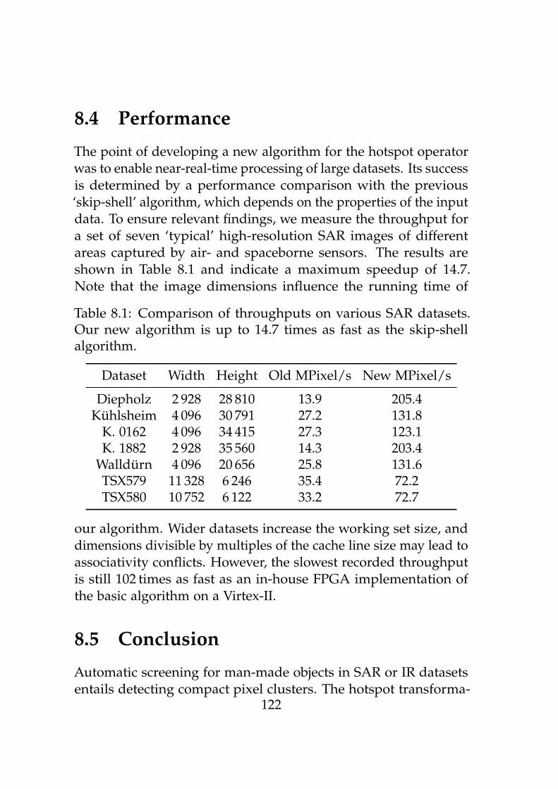
8.4 Performance

The point of developing a new algorithm for the hotspot operatorwas to enable near-real-time processing of large datasets. Its successis determined by a performance comparison with the previous‘skip-shell’ algorithm, which depends on the properties of the inputdata. To ensure relevant findings, we measure the throughput fora set of seven ‘typical’ high-resolution SAR images of differentareas captured by air- and spaceborne sensors. The results areshown in Table 8.1 and indicate a maximum speedup of 14.7.Note that the image dimensions influence the running time of

Table 8.1: Comparison of throughputs on various SAR datasets.Our new algorithm is up to 14.7 times as fast as the skip-shellalgorithm.

Dataset Width Height Old MPixel/s New MPixel/s

Diepholz 2 928 28 810 13.9 205.4Kühlsheim 4 096 30 791 27.2 131.8

K. 0162 4 096 34 415 27.3 123.1K. 1882 2 928 35 560 14.3 203.4

Walldürn 4 096 20 656 25.8 131.6TSX579 11 328 6 246 35.4 72.2TSX580 10 752 6 122 33.2 72.7

our algorithm. Wider datasets increase the working set size, anddimensions divisible by multiples of the cache line size may lead toassociativity conflicts. However, the slowest recorded throughputis still 102 times as fast as an in-house FPGA implementation ofthe basic algorithm on a Virtex-II.

8.5 Conclusion

Automatic screening for man-made objects in SAR or IR datasetsentails detecting compact pixel clusters. The hotspot transforma-

122

tion successfully suppresses other pixels, but is computationallyexpensive. We have introduced a new algorithm with linear com-plexity in the pixel count and object size, which is asymptoticallyoptimal. Our sophisticated implementation avoids redundant com-putations by means of a divide and conquer scheme and organizesits memory accesses so the working set fits in the cache. Paral-lelization and vectorization yield a combined 27-fold speedup. Asingle workstation is able to process 72 MPixel/s, which allowsrapid screening of large datasets. The algorithm is used as a pre-processing step for multi-class target recognition in MSTAR SARdata via support vector machine.

123

Chapter 9

Discussion

This work has described techniques for maximizing performanceon modern CPUs, namely vectorization, parallelization and ac-counting for the memory hierarchy. They have given rise to 10–100x speedups in seven separate algorithms, thus emphasizingtheir practical relevance and wide applicability. In several cases,the resulting software exceeds the reported performance of special-ized hardware. This provides somewhat unexpected input to thecurrent discussion of which computer architecture is suitable fora given task. General-purpose CPUs can still compare favorably,even when performance goals are ambitious. Although some ofour techniques are designed for specific microarchitectures, thepast has shown that their basic principles remain valid for a decadeor more.

The above conclusions stand for themselves, but our main objec-tive was to design and implement an efficient processing chain forimage analysis. Although this work does not constitute progress onunderstanding the image contents, nor realize a full-fledged demon-stration application, it provides useful building blocks for theincreasingly accepted object-based image analysis paradigm [194].We have introduced new algorithms for each step that significantlyoutperform previous approaches while maintaining high-qualityresults. This is important because modern imaging sensors deliverever-increasing amounts of data. Our results demonstrate the feasi-bility of processing aerial imagery of 100 km × 100 km areas at 1 m

125

resolution within minutes, which goes far beyond our initial goalof 2 hours.

Each link of the chain is designed as part of a coherent whole.For example, the pan sharpening algorithm arranges for edge-preserving smoothing to aid the subsequent segmentation, and ourimage I/O module includes support for statistics and tiled pixelformats to allow for better viewing of large images. The processingchain serves to shoulder the brunt of the expensive pixel-basedprocessing required for various image analysis tasks. Subsequentapplications need not be as concerned with performance, becausethey can draw upon a more compact and higher-level object-basedrepresentation of the image. This general approach of optimizingrelatively small modules responsible for most of the execution timeprovides major performance benefits at a reasonable cost.

However, much remains to be done. Building further appli-cations besides our change-detection prototype would indicatewhether the current set of image features is sufficient for a widerrange of tasks. In particular, extracting and simplifying segmentcontours would be helpful for matching and classifying objects. Wehave developed algorithm prototypes for both problems (includingvectorization of the inherently sequential polygon simplificationtask) that lead us to believe a throughput comparable to the rest ofthe processing chain may be attained.

Some applications also require accuracy guarantees. An anal-ysis of the maximum deviation in the pan-sharpening stage andan error model for the segmentation could prove useful. Both ofthese steps also require user-defined parameters for the degree ofsmoothing and minimum object contrast, respectively. It would behelpful to automatically derive both from the input datasets.

Returning once again to the general issue of performance,we believe that many of the techniques developed herein arebroadly applicable to other domains. For example, efficient asyn-chronous transfers can speed up I/O-intensive applications, includ-ing external-memory algorithms. An awareness of the memory

126

hierarchy, especially working set size and cache pollution, shouldimprove nearly any algorithm that frequently accesses memory.Finally, modern multi-core CPUs with SIMD instruction sets offera surprising degree of parallelism. The combination of optimizedalgorithms and a balanced architecture (including high single-coreperformance for the serial portion of parallel algorithms) can allowa CPU to remain competitive with other specialized architectures.

127

Part III

Desserts

129

Appendix A

Virtual-Memory Counting Sort

We present a fast radix sorting algorithm that builds upon amicroarchitecture-aware variant of counting sort. Taking advan-tage of virtual memory and making use of write-combining yieldsa per-pass throughput corresponding to at least 89% of the sys-tem’s peak memory bandwidth. Our implementation outperformsIntel’s recently published radix sort by a factor of 1.64. It alsocompares favorably to the reported performance of an algorithmfor Fermi GPUs when data-transfer overhead is included. These re-sults indicate that scalar, bandwidth-sensitive sorting algorithms re-main competitive on current architectures. Various other memory-intensive applications can benefit from the techniques describedherein.

This chapter has undergone minor revisions since its publica-tion at Euro-Par 2011 [195].

A.1 Introduction

Sorting is a fundamental operation that is a time-critical compo-nent of various applications such as databases and search engines.The well-known lower bound of Ω(n log n) for comparison-basedalgorithms no longer applies when special properties of the keyscan be assumed. In this work, we focus on 32-bit integer keys,optionally paired with a 32-bit (or larger) value. This simplifies the

131

implementation without loss of generality, because applicationscan often replace large records with a pointer or index [196]. Theradix sort algorithm is commonly used in such cases due to itsO(n) complexity. In this report, we present a 1.64-fold performanceincrease over results recently published by Intel [197].

The remaining sections are organized in a bottom-up fashion,with Section A.2 dedicated to the basic realities of current andfuture microarchitectures that affect memory-intensive programsand motivate our approach. We build upon this foundation inSection A.3, showing how to speed up counting sort by takingadvantage of virtual memory and write-combining. Section A.4applies this technique towards a novel variant of radix sort. The per-formance of our implementation is evaluated in Section A.5. Band-width measurements indicate the per-pass throughput is nearlyoptimal for the given hardware. Its two CPUs outperform a FermiGPU when accounting for data-transfer overhead.

A.2 Software Write-Combining

We begin with a description of basic microarchitectural realities thatare likely to have a serious impact on applications with numerousmemory accesses, and show how to avoid performance penaltiesby means of Software Write-Combining. These topics are not new,but we believe they are often not adequately addressed.

The first problem arises when writing items to multiple streams.An ideal cache with at least as many lines could exploit the writes’spatial locality and entirely avoid non-compulsory misses. How-ever, perfect hit rates are not achievable in practice due to limitedways of associativity a [198]. Because only a lines can be mappedto a cache set, any further allocations from that set would result inthe eviction of one of the previous lines. If possible, applicationsshould avoid writing to many different streams. Otherwise, thevarious write positions should map to different sets to avoid thrash-ing and conflict misses. For current L1 caches with a = 8 ways, size

132

C = 32 KiB and lines of B = 64 bytes, there are S = CaB = 64 sets,

and bits [lg B, lg B + lg S) of the destination addresses should dif-fer (e.g. by ensuring the write positions are not a multiple ofSB = 4 KiB apart).

A second issue is provoked by a large number of write-onlyaccesses. Even if an entire cache line is to be written, the previousdestination memory must first be read into the cache. Althoughthe corresponding latency may be partially hidden via prefetch-ing, the cache line allocations remain problematic due to capacityconstraints and eviction policy. Instead of displacing write-onlylines that are not accessed after having been filled, the widespread(pseudo-)Least-Recently-Used strategy displaces previously cacheddata due to their older timestamp. An attempt to avoid theseevictions by explicitly invalidating cache lines (e.g. with the IA-32CLFLUSH instruction) did not yield meaningful improvements.Instead, applications should use non-temporal streaming store instruc-tions that write directly to memory, thus avoiding cache pollutionbecause they circumvent the cache.

This leads directly to the next concern: single memory accessesinvolve significant bus overhead. The architecture therefore com-bines neighboring non-temporal writes into a single burst transfer.However, currently microarchitectures only provide four to tenwrite-combine (WC) buffers [199]. Non-temporal writes to multi-ple streams may force these buffers to be flushed to memory via‘partial writes’ before they are full. The application can preventthis by making use of Software Write-Combining [200]. The datato be written is first placed into temporary buffers, which almostcertainly reside in the cache because they are frequently accessed.When full, a buffer is copied to the actual destination via consec-utive non-temporal writes, which are guaranteed to be combinedinto a single burst transfer.

This scheme avoids reading the destination memory, whichmay incur relatively expensive Read-For-Ownership transactionsand would only pollute the cache. It works around the limited

133

number of WC buffers by using L1 cache lines for that purpose.Interestingly, this is tantamount to direct software control of thetransparently managed cache.

We recommend the use of such Software Write-Combiningwhenever a core’s active write destinations outnumber its write-combine buffers. Fortunately, this can be done at a fairly highlevel, because only the buffer copying requires special vector loadsand non-temporal stores (which are best expressed by the SSE2intrinsics built into the major compilers).

A.3 Virtual-Memory Counting Sort

We now review Counting Sort of n elements with keys in [0, m) anddescribe an improved variant that makes use of virtual memoryand write-combining.

The naïve algorithm first generates a histogram of the n keys.After computing the prefix sum to yield the starting output locationfor each key, each value is written at its key’s output position, whichis subsequently incremented.

Our first optimization goal is to avoid the initial counting pass.We could instead insert each value into a per-key container, e.g.a list of data blocks. However, this incurs some overhead forchecking whether the current bucket is full. Preallocating spacefor m arrays of size n is more efficient, because items can simplybe written to the next free position (c.f. Algorithm A.1, introducedin [201]). This algorithm only writes and reads each item once,a feat that comes at the price of nm space. Although this appearsproblematic in the Random-Access-Machine model, it is easilyhandled by 64-bit CPUs with virtual memory organized into pagesof size p. Physical memory is only mapped to pages when they arefirst accessed1, thus reducing the actual memory requirements to

1Accesses to non-present pages result in a page fault exception. The applicationreceives such events via signals (POSIX) or Vectored Exception Handling (Windows)and reacts by committing memory, after which the faulting instruction is repeated.

134

Algorithm A.1: Single-pass counting sort1 storage := ReserveAddressSpace(nm);2 for i := 0 to m− 1 do next [i] := in;3 foreach key,value do4 storage [next [key]] := value;5 next [key] := next [key] + 1;6 end

O(n + mp). The remainder of the initial allocation only occupiesaddress space, of which multiple terabytes are available on 64-bitsystems.

Having avoided the initial counting pass, we now show howto efficiently write values to storage using the write-combiningtechnique described in Section A.2. Our implementation initializesthe next pointers to consecutive, naturally aligned, cache-line-sizedbuffers. A buffer is full when its (post-incremented) position isevenly divisible by its size. When that happens, an unrolled loopof non-temporal writes copies the buffer to its key’s current outputposition within storage. These output positions are also stored inan array of pointers.

A.4 Radix Sort

After a brief review of radix sorting, we introduce a new vari-ant based on the virtual-memory counting sort described in Sec-tion A.3.

A radix sort successively examines D-bit ‘digits’ of the K-bitkeys. They are characterized by the order in which digits areprocessed: starting at the Least Significant Digit (LSD), or MostSignificant Digit (MSD).

An MSD radix sort partitions the items according to the currentdigit, then recursively sorts the resulting buckets. Although it nolonger needs to move items whose previously seen key digits are

135

unique, this is not especially helpful when the number of passesK/D is small. In fact, the overhead of managing numerous (nearlyempty) buckets makes MSD radix sort less suited for relativelysmall n.

By contrast, each iteration of the LSD variant partitions all itemsinto buckets by the current key digit. This amortizes the bucketsetup cost over the number of elements and avoids the possibilityof load imbalance for parallelization at the price of increased datacopying.

To reduce this overhead and also parallel communication, wemake use of “reverse sorting” [202], in which one or more MSDpasses partition the data into buckets, which are then locally sortedvia LSD. This turns out to be even more advantageous for NUMAsystems because each processor is responsible for writing a contigu-ous range of outputs, thus ensuring the operating system allocatesthose pages from the processor’s NUMA node [193].

Let us now examine the pseudocode of the radix sort (Algo-rithm A.2), choosing K = 32 for brevity and D = 8 to allowextracting key digits without masking. Each Processing Element(PE) first uses counting sort to partition its items into local bucketsby the MSD (digit = 3). Note that items consist of a key and value,which are adjacent in memory (ideally within a native 64-bit word,but larger combinations are possible in our implementation vialarger user-defined types). When all are finished, the output indexof the first item of a given MSD is computed via prefix sum. EachPE is assigned a range of MSD values, sorting the buckets fromall PEs for each value. Skewed MSD distributions can cause loadimbalance. However, this could be resolved via special treatmentof large buckets2. The local sort entails K/D− 1 iterations in LSDorder. The first copies all other PEs’ buckets into local memory. Thesecond to last pass also computes the last digit’s histogram, whichallows writing directly to the output positions in the final pass.Note that three sets of buckets are required, which makes heavy

2Sorting buckets larger than n/|PE| using multiple PEs.

136

Algorithm A.2: Parallel Radix Sort1 parallel foreach item do2 d := Digit(item, 3);3 buckets3 [d] := buckets3 [d] ∪ item;4

5 Barrier;6 foreach i ∈

[0, 2D

)do

7 bucketSizes [i] := ∑PE |buckets3 [i]|;8 end9 outputIndices := PrefixSum(bucketSizes);

10 parallel foreach bucket3 ∈ buckets3 do11 foreach item ∈ bucket3 ∀PE do12 d := Digit(item, 0);13 buckets0 [d] := buckets0 [d] ∪ item;14 end15 foreach bucket0 ∈ buckets0 do16 foreach item ∈ bucket0 do17 d := Digit(item, 1);18 buckets1 [d] := buckets1 [d] ∪ item;19 d := Digit(item, 2);20 histogram2 [d] := histogram2 [d] + 1;21 end22 end23 foreach bucket1 ∈ buckets1 do24 foreach item ∈ bucket1 do25 d := Digit(item, 2);26 i := outputIndices [d] + histogram2 [d];27 histogram2 [d] := histogram2 [d] + 1;28 outputArray [i] := item;29 end30 end31

137

use of virtual memory (3× 2D × |PE| = 6144 times the input size).Whereas 64-bit Linux grants each process 128 TiB address space,Windows limits this to 8 TiB, which means only about 1.4 GiB ofinputs can be sorted3.

We briefly discuss additional system-specific considerations.The radix 2D was motivated by easy access to each digit, but is alsolimited by the cache and TLB size. Because of the many requiredTLB entries, we map the buckets with small pages, for which theIntel i7 microarchitecture has 512 second-level TLB entries. Toincrease TLB coverage, we use large pages for the inputs. Theworking set consists of 2D buffers, buffer pointers, output positions,and 32-bit histogram counters. This fits in a 32 KiB L1 data cache ifthe software write-combine buffers are limited to a single 64-bytecache line. To avoid associativity and aliasing conflicts, these arraysare contiguous in memory. Interestingly, these optimizations donot detract from the readability of the source code. Knowledgeof the microarchitecture can also be applied towards middle-levellanguages and enables principled design decisions.

A.5 Performance

We characterize the performance of our sorting implementa-tion by its throughput, defined as n

t1−t0, where n is the num-

ber of items and t0 and t1 are the earliest and latest start andfinish times reported by any thread. The test platform con-sists of dual W5580 CPUs (3.2 GHz, 48 GiB DDR3-1066 mem-ory) running Windows XP x64. Our implementation is compiledwith ICC 11.1.082 /Ox /Og /Oi /Ot /Qipo /GA /GR- /GS- /EHsc

/Qopenmp /QaxSSE4.2. When sorting 350 M uniformly distributed32-bit keys generated by the WELL512 algorithm [203], the basicalgorithm (‘VM only’) reaches a throughput of 391 M items/s, as

3This limitation could be circumvented by estimating bounds for bucket sizes viasampling. In the unlikely case that they are exceeded, a new sample would be drawnand the process repeated.

138

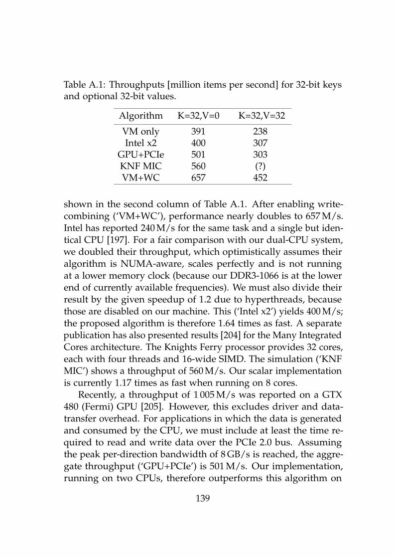
Table A.1: Throughputs [million items per second] for 32-bit keysand optional 32-bit values.

Algorithm K=32,V=0 K=32,V=32

VM only 391 238Intel x2 400 307

GPU+PCIe 501 303KNF MIC 560 (?)VM+WC 657 452

shown in the second column of Table A.1. After enabling write-combining (‘VM+WC’), performance nearly doubles to 657 M/s.Intel has reported 240 M/s for the same task and a single but iden-tical CPU [197]. For a fair comparison with our dual-CPU system,we doubled their throughput, which optimistically assumes theiralgorithm is NUMA-aware, scales perfectly and is not runningat a lower memory clock (because our DDR3-1066 is at the lowerend of currently available frequencies). We must also divide theirresult by the given speedup of 1.2 due to hyperthreads, becausethose are disabled on our machine. This (‘Intel x2’) yields 400 M/s;the proposed algorithm is therefore 1.64 times as fast. A separatepublication has also presented results [204] for the Many IntegratedCores architecture. The Knights Ferry processor provides 32 cores,each with four threads and 16-wide SIMD. The simulation (‘KNFMIC’) shows a throughput of 560 M/s. Our scalar implementationis currently 1.17 times as fast when running on 8 cores.

Recently, a throughput of 1 005 M/s was reported on a GTX480 (Fermi) GPU [205]. However, this excludes driver and data-transfer overhead. For applications in which the data is generatedand consumed by the CPU, we must include at least the time re-quired to read and write data over the PCIe 2.0 bus. Assumingthe peak per-direction bandwidth of 8 GB/s is reached, the aggre-gate throughput (‘GPU+PCIe’) is 501 M/s. Our implementation,running on two CPUs, therefore outperforms this algorithm on

139

a current top-of-the-line GPU by a factor of 1.31 despite lowertransistor counts (2× 731 M vs. 3 000 M) and thermal design power(2× 130 W vs. 275–300 W).

Similar measurements and extrapolations for the case of 32-bit keys associated with V = 32-bit values are given in the thirdcolumn of Table A.1. Because the slowdown is less than a factorof two, the implementations are at least partially limited by com-putation instead of bandwidth. Intel’s algorithm is more efficientin this regard, with only a 1.3-fold decrease vs. our factor of 1.45.The additional data transfers over PCIe render the GPU algorithmuncompetitive.

Because radix sort is bandwidth-sensitive, it is also interestingto examine performance for a varying number of processors. Wemanually distribute OpenMP threads across CPU packages andcores (in that order) to make use of all available memory controllers.Our NUMA-aware implementation scales linearly with the numberof threads, as shown by Figure A.1. To explain the 95% parallelefficiency, we measured the total traffic at each socket’s memorycontroller. Because this information is not available from currentprofilers such as VTune (which use per-core performance coun-ters), we have developed a small kernel-mode driver to provideaccess to the model-specific performance counters in the Intel i7uncore4. Uncached writes constitute the bulk of the write combin-ers’ memory traffic and are therefore of particular interest. Theyare apparently reported as Invalid-To-Exclusive transitions andcan thus be counted as the total number of reads minus ‘normal’reads [206]. We find that 2 041 MiB are written, which correspondsto 64 Mi items × 8 bytes per item × 4 passes (slightly less becauseour final pass cannot use non-temporal writes when the output po-sition is not aligned). Surprisingly, 2 272 MiB are read – about 10%more than expected. This amount seems to be influenced by thenumber of threads. Possible causes may include coherency trafficor page walks and will be investigated in future work. However,

4The part of the socket not associated with a particular core.

140

1 2 3 4 5 6 7 81

2

3

4

5

6

7

8

Number of threads

Spee

dup

vs.s

ingl

eth

read

Figure A.1: Linear scalability on two quad-core CPUs with aNUMA factor of 1.5.

we can provide a conservative estimate of the bandwidth utiliza-tion. Given the pure read and write bandwidths (38 687 MB/s and28 200 MB/s) measured by RightMark [153], the minimum timerequired for 4 reads and writes of 175 M 8-byte items is 343 ms,which is 89% of the total measured time. This calculation does notinclude write-to-read turnaround [207, p. 486], so there is even lessroom for improvement than indicated.

The previous measurements concern large numbers of items.We now study performance over a wider range of input sizes. Theelapsed time per item, shown in Figure A.2, varies inversely withthe number of items n due to amortization of thread-startup over-head. Performance is within 10% of the best measurement whenn ≥ 26 Mi, or n ≥ 21 Mi in the case of the approximated Gaussiandistribution [208]. It is initially surprising that this distribution

141

does not require more time to sort than uniformly distributed num-bers. However, interleaving buckets in the LSD passes (successivebuckets are assigned to different threads) reduces load imbalance,and increased occupancy of the central buckets improves localityat the memory page level.

50 100 150 200 250 3001.5

1.52

1.54

1.56

1.58

1.6

1.62

1.64

1.66

1.68

1.7

Number of 32-bit items [×20]

Nan

osec

onds

per

item Uniform

Gaussian

Figure A.2: Time per item for various input sizes and distributions.

A.6 Conclusion

We have introduced improvements to counting sort and a novelvariant of radix sort for integer key/value pairs. Bandwidth mea-surements indicate our algorithm’s throughput is within 11% of

142

the theoretical optimum for the given hardware. It outperformsthe recently published results of Intel’s radix sort by a factor of1.64 and also outpaces a Fermi GPU when data transfer overheadis included. These results indicate that scalar, bandwidth-sensitivesorting algorithms still have their place on current architectures.However, achieving this level of performance requires awareness ofthe underlying microarchitecture and some degree of tuning. Ourimplementation encompasses 5 700 lines of C++ (including tests),plus 40 000 lines of shared infrastructure. A demo executable [209]capable of generating or reading 32-bit integers, sorting and effi-ciently writing them to disk is being made available so that ourmeasurements may be reproduced.

Future Work. Although carefully engineered, our implementa-tion is not yet a general solution for all possible sorting applications.Radix sort is limited to relatively small integer keys, and we also as-sume at least one of the key digits (e.g. MSB) is reasonably equallydistributed. Skewed (e.g. constant) distributions currently result inload imbalance. This could be avoided by sorting extremely largebuckets from the MSD phase using multiple processors.

We are also interested in testing on larger multi-socket ma-chines with higher NUMA factors5 and investigating details ofthe memory subsystem that reduce effective bandwidth. Finally,we believe the general software write-combining technique canprovide similar speedups for other memory-intensive applications.In particular, comparison-based sample sort is also expected tobenefit from our implementation techniques.

5The ratio between remote and local memory latency.

143

Appendix B

Implementation Details

B.1 Software Engineering

Building the image processing chains described in this work fromthe ground up was a sizable undertaking spanning 2008–2011. Theauthor developed over 100 000 lines of C++ code (LOC), whichare organized into 12 dynamic-link libraries to avoid repetitivecompilation. This allows a full rebuild of optimized binaries within90 s using the Intel compiler on a 12-core system equipped withan SSD. The Microsoft Visual Studio 2010 integrated developmentenvironment (IDE) is augmented with Intel’s Parallel Studio 2011,which encompasses a compiler, tools for detecting race conditionsor memory errors, and a profiler (formerly known as VTune) formeasuring where execution time is spent and reading the proces-sor’s performance counters.

Eight standalone applications have been developed for testingthe modules in isolation. The Subversion (SVN) software con-figuration management system was used to maintain versioninginformation, recording a total of 38 992 file changes in 2 767 revi-sions. Besides providing information security, this was valuablefor showing what changed since the last known-good version andreverting edits made during failed experiments. Extensive pre- andpostcondition checks and self-tests built into the software exposedmany errors early on. A custom ASSERT macro enabled easier

145

analysis of the problem (even in optimized builds) by displayingerror messages with a record of the previously called subroutinesand the values of their local variables.

As mentioned in Section 4.2, we use special C++ functions(‘SIMD intrinsics’) and classes provided by the compiler to generateSIMD code. Please refer to the commented source code of the linerasterizer [173] for a complete example of their syntax and somelow-level optimization techniques.

B.2 Unaligned Memory Accesses

It was mentioned in Section 8.4 that vectorization of the hotspotoperator yields a surprisingly low speedup and that the cause isrelated to Intel CPUs’ poor handling of unaligned memory accesses.Because this issue seriously impacts performance and is likely toaffect other applications as well, we will now delve into the details.A preliminary version of this section appeared in [186].

The Intel Core 2 microarchitecture delays SIMD load operationsthat cross a cache line boundary (‘splits’) [53, p. 83] by 12 cycles.This issue is documented in [200, p. 5-38], which recommends us-ing LDDQU1 to load two aligned vectors and shift the data into place,thus avoiding a cache line split. An unfortunate design trade-off inthe Core 2 microarchitecture has replaced the implementation ofthis instruction with that of the architecturally equivalent MOVDQU2,which remains affected by splits. The newer Intel i7 microarchitec-ture reduces the cost of splits to 2 cycles.

In the meantime, several workarounds have been attempted forthe hotspot operator: substituting two 64-bit loads to decrease theprobability of splits is consistently 4% slower. Using PALIGNR3 toemulate LDDQU works but requires the misalignment to be known

1LoaD Double-Quad Unaligned.2MOVe Double-Quad Unaligned.3Packed ALIGN Right.

146

at compile-time. Realizing that access patterns for each intervallength are fixed, several ShellMax functions were generated viatemplates and called through function pointers. This turns out tobe 20% slower, probably due to mis-predicted indirect branches. Afinal alternative lies in manually aligning accesses, which is feasiblebecause shell maxima computations only require three distinctmisalignments. Unfortunately the SSE instruction set does notallow variable shifts of full registers and restricting all operationsto the lower halves of registers decreases performance by about25%. Regardless, the cost of two aligned loads, two shift and oneOR-operation vastly outweighs the expense of cache line splits. Itappears that straightforward use of MOVDQU is currently the bestoption, especially because AMD microarchitectures also handleunaligned loads with only slight penalties.

We now show the performance impact of cache line and pagesplits on Core 2 CPUs in the context of the hotspot operator. As-suming 2-byte values and 64-byte L1D cache lines, 7 out of the32 possible misalignments should cross a cache line boundary.Instrumentation shows that the actual number is 22.13%. This isslightly more than expected because the misalignments are notquite uniformly distributed. Similar arguments apply for pagesplits; assuming sizes of 4 KiB, we expect a ratio of 7 out of 2 048and observe 0.34%, which is in good agreement. Using the per-splitcosts of 12 and 224 cycles given in [210] and supposing a 3 GHzprocessor, we therefore expect 1.42 s of CPU time to be lost due tothe splits. A variant of the hotspot algorithm that rounds downall addresses to their natural alignment runs 1.33 s faster than thenormal single-core version. This measurement matches the aboveprediction save for a slight difference due to the overhead of mask-ing the lower address bits. Cacheline- and page split penaltieshave therefore been shown to be responsible for increasing totalcomputation from 2 223 ms to 3 641 ms, i.e. a factor of 1.63!

To gain a better understanding of the cause, we have used theVTune profiler to observe certain CPU performance counters. The

147

first surprising observation is a large amount of L1D misses despitethe fact that these accesses are local. This and a cache line splitpenalty equal to the L2 access latency leads to the presumption thatsuch loads are simply not serviced by the L1 cache and must gothrough L2. Page splits apparently have a different effect becausethey do not cause an excessive amount of L2 misses. Insteadwe note a significant number of TLB misses even though largepages are used and working set does not exceed TLB capacity.This seems to point towards page splits requiring a page walk,especially because the overhead is similar to that reported in [42, p.21]. These findings are in accordance with [210].

Although the above discussion may be deemed highly system-specific, it is also quite relevant for real-world performance. Itis safe to say that processors will generally — and perhaps to asurprising degree — penalize unaligned memory accesses. Becauseaccess patterns are intimately tied to the design of algorithms, thisissue must be kept in mind during their design.

B.3 LVT File Format

Section 3.3 stated our requirements for an image file format, par-ticularly integer and floating-point data types, compression, tiling,image pyramids and flexible metadata. We are not aware of anexisting format that covers these needs, aligns data for efficientaccess and avoids conversion overhead. This has motivated thedevelopment of a new Lossless Virtual Texture (LVT) layout. Letus emphasize that it is not intended to replace existing formats.Instead, it can be seen as an optimized alternate representation thatprovides rapid access to image tiles, thus enabling smooth naviga-tion and zooming within the full-resolution pixels. Its high-levelstructure is straightforward: the image tiles are followed by anarbitrary number of variable-sized ‘sections’ containing metadata.

148

In the following, we provide precise definitions of these compo-nents and our design rationale. The data structures are describedvia C++ syntax, with u8, u16, u32 and u64 respectively denotingunsigned 8, 16, 32 and 64-bit integer fields.

Tiled Pyramid

To allow smooth navigation within large images at low zoom scales,the format provides for a multi-resolution pyramid of ‘levels’. Level0 is defined as the original image embedded within a square whosedimensions are a power of two. Subsequent levels are half as wideand high as their predecessor. Each level is split into individualtiles. We truncate the pyramid after a level fits into a single tilebecause subsequent levels are never used.

It is important to carefully arrange tiles to improve locality andenable a parallel external-memory algorithm for computing thepyramid from the original image. A level’s tiles can be orderedaccording to a 2-D Space Filling Curve (SFC) [211], thus decreasingthe average distance of nearby tiles within the file, which mayreduce the number and cost of disk seeks. A 3-D mapping obtainedby including the level would be wasteful, because the pyramidonly fills a small part of the 3-D space. By contrast, contiguous tileindices (the number corresponding to a tile’s position on the space-filling curve) would allow simple and efficient lookups of a tile’slocation. More importantly, defining the curve to match the orderin which higher-level tiles are generated from their predecessorswould minimize memory use when creating the image pyramid.We introduce a novel mapping with both of these properties.

Consider a 2× 2 quartet of level 0 tiles, denoted ‘quad’, fromwhich one level 1 tile may be computed via downsampling. Af-terwards, the quad’s four tiles are no longer needed and may beremoved from memory once they have been written to the file. Thecurve we seek must first visit the quad, the resulting level 1 tile,three other neighboring quads and their level 1 tiles, and then the

149

resulting level 2 tile. Let us begin with a 2-D Z-order curve (the‘Peano’ curve of [211] rotated 90 degrees clockwise). In accordancewith standard practice, we transform X and Y coordinates to a Zindex by interleaving their bits via SIMD [212]. The resulting valueis shifted left by dlog(numLevels+ 3)e bits. In the lower bits,we encode either the quadrant [0,3] of the level 0 tiles, or 3 plusthe level index of any higher-level tiles generated from the quad.Indices of tiles above level 0 are offset by the cumulative sum ofthe distance between Z neighbors in previous levels, thus shapingthe 3-D space into a pyramid. A tile at level i + 1 immediatelyfollows the level i tile that is its fourth and final quadrant, whichis the desired property that allows constructing the pyramid withminimal memory use.

Tiles are stored in the order induced by this curve. Dependingon the tileEncoding field, each either consists of uncompressed,band-interleaved pixels, or the compressed variable-length LASCrepresentation of them. Because the next tile’s offset is determinedfrom its predecessor’s size, the tiles are stored back-to-back. Thisrequires a parallel compression pipeline to stall until the sizes of allpreceding tiles are known. We prefer the resulting slight increasein compression time over larger file sizes because generating large-scale images is usually an off-line process.

Sections

Metadata within the file is organized into variable-length ‘sections’.Each is identified by a four-character code. Applications may definefor their own use any sequence beginning with ‘~’ and continuingwith three uppercase letters. This definition of the LVT file formatincludes six built-in section types, which shall be discussed in turn.

150

LVTD

To allow rapid localization of sections without incurring expensivehard-disk seek operations, version 3 of the “LVTD” section is adirectory of fixed-length entries – one per section, including its own.Entries must be sorted by increasing file offset, and the directorymust reside immediately prior to the end of the file. The numberof entries is derived from the section size, and each includes thefollowing fields:

u8 identifier[4];u32 version;u32 encoding;u32 checksum;u64 size;u64 offset;

identifier is an application-defined character sequence or oneof the paragraph headings in this text. version indicates theversion number of the section definition. Because the format is in-tended as a simple intermediate representation, we do not providefor backward nor forward compatibility. A 32-bit integer is largerthan necessary, but we prefer to use a processor’s native integertype to avoid more complicated instruction encodings for softwarereading the fields. encoding must be 0, indicating the section isuncompressed. checksum must be 0 and is reserved for possibleverification of section integrity in future versions. size indicatesthe length [bytes] of the actual section. offset points to its lo-cation in the file. To simplify asynchronous I/O (c.f. Section 3.2),both of these values must be a multiple of sectionAlignment,which is currently 4 KiB. 64-bit integers avoid restrictions on thesize and position of sections in large files. Note the deliberatepower-of-two size of the directory entries, which simplifies addresscomputations.

151

PARA

Version 3 of the “PARA” section indicates the parameters thatgoverned the creation of the LVT file:

u32 interpolation;u32 tileEncoding;float noDataValue;float ignoreValue;u32 binFunction;u32 numThreads;

interpolation specifies the interpolation method when down-sampling: nearest neighbor (0) or bilinear (1). tileEncoding in-dicates whether tiles are uncompressed (0) or encoded with LASC(1), described in Chapter 4. noDataValue is the pixel componentvalue used to initialize pixels that lie outside the original image.Tiles whose pixel components are all equal to this value are omit-ted from the file. Setting it in accordance with the most commonluminance in the image may reduce the file size. ignoreValueallows ignoring all pixel components with a certain value whencomputing statistics. To avoid this, specify an ‘impossible’ valuethat does not occur in the image. binFunction indicates whetherthe histogram bin function is linear (0) or logarithmic (1) with basee. numThreads specifies the maximum number of threads in theparallel pipeline for computing the image pyramid. This valueis of no use to readers of an LVT file, but is written to disk forconvenience.

STAT

Version 1 of the “STAT” section begins with basic image character-istics: u32 width, height, pixelFormat;width and height indicate the number of valid pixels in eachdimension, which need not be a multiple of tileDim (256).

152

pixelFormat is a convenient and compact encoding of the ‘com-ponent type’ (the representation of a digital number indicating theintensity within a spectral band for each pixel) and the number ofcomponents per pixel. The size of the component type is storedwithin the lower 8 bits to allow efficient computation of storagerequirements. To distinguish between 32-bit integers and single-precision floating-point numbers, exactly one of three additionalbits must be set. Bit 15 (32 768) indicates an unsigned integer, bit 14denotes a signed integer and bit 13 signals a floating-point number.The number of components (up to 4 096) is stored in bits 16 andabove. The section also stores statistics for each band:

float ignoreValue;u64 numIgnored;double min, max, mean, stddev, median, mode;u64 histogram[256];

ignoreValue specifies the value of a component to ignore whencomputing the statistics. This is useful for images with backgroundor no-data areas, which would otherwise affect the mean value. Toavoid branching or code duplication, this functionality is alwayspresent. However, it can effectively be disabled by specifying ‘im-possible’ values such as infinity. numIgnored counts the numberof components that were ignored. min and max are the minimumand maximum component values encountered. They are initializedto the largest positive and smallest negative value representableas a double, respectively, and remain unchanged if all values areignored. mean, stddev (standard deviation) and median are theeponymous statistical measures. mode is the most frequent value,computed as the lower bound of the histogram bin whose count isthe largest. histogram indicates how many components’ valuesfall into each of its bins, which are equal-width subdivisions of theinterval [min, max]. The use of 64-bit integers avoids overflow andinexact counts.

153

RANG

Version 6 of the “RANG” section is a compressed representation ofthe range (i.e. offset and size) each tile occupies in the file. Becausetile sizes are always multiples of tileAlignment (which againcorresponds to the minimum 4 KiB sector size), we divide by thatvalue and store the results in unsigned 16-bit integers referred to asquantized sizes. Tile indices include small gaps of unused valuesbecause not all quads generate tiles of levels > 1. To avoid storingranges for such indices, we introduce ‘groups’ of quads denotedQuadGroup. The data structure describing them is designed to fitwithin a single cache line:

u64 firstTileOffset;u16 quadSizes[4];u16 tileSizes[24];

firstTileOffset is the file offset of the first tile in this group.Being a multiple of tileAlignment, we let the lower 12 bitsdenote whether this group includes tiles of level > 5. quadSizesare the quantized total sizes of each quad in the group. tileSizesstores the quantized sizes of 4+1 tiles in 3 quads, and a total of4+5 tiles’ sizes for the last quad, because it is the only one thatmay generate multiple higher-level tiles. The offset of a tile of agiven index is retrieved by advancing to the group’s first offset,skipping past prior quads within the group and then previous tilesinside the quad. If the tile’s level does not exceed the array capacity,its size is also retrieved from tileSizes. Otherwise, the tile isassumed to be uncompressed and its size is computed from theimage pixel format. However, the lower bits of firstTileOffsetallow eliding tiles whose pixels are all equal to the no-data value;their sizes are considered to be zero.

Although QuadGroup minimizes wasted space due to non-present high-level tiles, embedding images within a square power-of-two grid for the sake of simple Z coordinate computation may

154

also lead to large ranges of unused indices. We mitigate this withan additional QuadChunk data structure:

u64 firstGroupOffset;u64 unused;u16 sizes[8];u32 validGroups[8];

firstGroupOffset is the offset of the first of eight 32-groupclusters that constitute a chunk. sizes holds the total sizes ofeach cluster. validGroups is a bit field indicating which of eachcluster’s groups are present. The QuadGroup governing a giventile is located by starting at the first offset, skipping previous clus-ters and then adding the size of QuadGroup times the number ofprior nonzero bits in the cluster’s validGroups field. This datastructure enables 256-fold compression of unused QuadGroup atthe expense of a single cache-line access and some minor com-putation. The “RANG” section consists of QuadChunk instancescovering all possible tile indices followed by as many QuadGroupas needed.

PROJ

To allow associating pixels with geographic coordinates, version 1of the optional “PROJ” section stores information about the mapprojection:

double ulx, uly, lrx, lry;i32 zone;char band;

ul and lr denote the upper-left and lower-right corners, forwhich we store x and y coordinates. zone is -1 if the othervalues are invalid/unknown, -2 to indicate the coordinates arelatitude/longitude, or a zone in [1, 60] for Universal TransverseMercator (UTM) coordinate systems. band is ‘?’ if unknown,otherwise a Military Grid Reference System (MGRS) latitude band.

155

CELL

Version 2 of the optional “CELL” section provides support for com-bining presentation slides or other pictures into one large image.This allows zooming in on individual slides without requiringseparate LVT files. Each slide resides in a square ‘cell’, and the im-age consists of a square cell matrix with power-of-two dimensions.Cells are described by the following:

u32 flags;u32 cellDim;u32 upperLeftX, upperLeftY;u32 elementWidth, elementHeight;u32 marginLeft, marginUpper;

flags has bit 0 set if the cell should not be zoomed. cellDimindicates the width and height in pixels of the cell, and must bedivisible by tileDim. Each cell must have the same dimension.upperLeftX and upperLeftY are the coordinates of the cell’stop left pixel within the entire image and are therefore multiples ofcellDim. Cells are arranged according to a ‘C-Scan’ [211]. Rowsalternate between left to right and right to left ordering; this enablesa simple sliding transition animation without bringing any othercells into view. elementWidth and elementHeight describethe size (in pixels) of the image that is embedded within the celland must not exceed cellDim. marginLeft and marginUpperindicate the number of no-data pixels on the left and upper borderof the cell. They must be non-zero multiples of tileDim.

Concluding Notes

The LVT file format has been designed for efficiency and flexibility,including a multitude of pixel formats. Extensibility is ensuredvia versioning and allowing for additional application-definedmetadata. Storing a tiled pyramid allows smooth navigation in

156

terapixel-scale images. A novel space-filling curve minimizes mem-ory requirements when creating the pyramid, which is writtensequentially without any disk seeks.

An awareness of low-level alignment issues reduces overhead.Each section and tile resides in its own disk sector, thus enablingdirect I/O without additional copying (c.f. Section 3.2). This alsoensures the SIMD alignment requirements are met when decom-pressing tiles. A compact directory avoids seeks when findingsections. The compressed tile lookup data structure allows re-trieving the size of any tile after only two cache line accesses andmodest computation.

It was a pleasure to design a capable, yet simple and highlyefficient layout that avoids the shortcomings of previous formats.Although chiefly intended as an optimized internal representationfor an image viewer, its efficiency may also lend itself to otherapplications.

157

Bibliography

[1] C. Bohren and A. Fraser. Colors of the sky. ThePhysics Teacher, pages 267–272, May 1985. Avail-able from: http://homepages.wmich.edu/~korista/colors_of_the_sky-Bohren_Fraser.pdf.

[2] Y. Chan and V. Koo. An introduction to synthetic apertureradar (SAR). Progress In Electromagnetics Research B, 2:27–60,2008.

[3] DigitalGlobe. DigitalGlobe core imagery products guide.Available from: http://www.digitalglobe.com/digitalglobe2/file.php/811/DigitalGlobe_Core_Imagery_Products_Guide.pdf.

[4] J. Pike. National image interpretability rating scales, Jan-uary 1998. Available from: http://www.fas.org/irp/imint/niirs.htm.

[5] K. Jacobsen. Recent developments of digital cam-eras and space imagery, January 2011. Availablefrom: http://www.ipi.uni-hannover.de/uploads/tx_tkpublikationen/2011_GISOSTRAVA_KJ.pdf.

[6] I. Niemeyer, S. Nussbaum, and M. Canty. Automation ofchange detection procedures for nuclear safeguards-relatedmonitoring purposes. In Geoscience and Remote SensingSymposium, 2005. IGARSS ’05. Proceedings. 2005 IEEE In-ternational, volume 3, pages 2133–2136, July 2005. doi:10.1109/IGARSS.2005.1526439.

159

[7] E. Bjorgo. United aid from the sky – a framework paper oncurrent and potential use of satellite imagery in united na-tions humanitarian organizations, April 2001. Available from:http://www.humanitarianinfo.org/imtoolbox/03_Mapping_GIS_GPS/Mapping_Reference/Remote_Sensing_Imagery/2001_UN_Remote_Sensing.doc.

[8] S. Smith. The Scientist and Engineer’s Guide to Digital SignalProcessing. California Technical Publishing, 1997. Availablefrom: http://www.dspguide.com/.

[9] J. Nickolls and W. Dally. The GPU computing era. IEEEMicro, 30(2):56–69, 2010. Available from: http://doi.ieeecomputersociety.org/10.1109/MM.2010.41.

[10] ELPIDA. Introduction to GDDR5, March 2010. Availablefrom: http://www.elpida.com/pdfs/E1600E10.pdf.

[11] D. Patterson. The top 10 innovations in the new NVIDIAFermi architecture, and the top 3 next challenges, Septem-ber 2009. Available from: http://www.nvidia.com/content/PDF/fermi_white_papers/D.Patterson_Top10InnovationsInNVIDIAFermi.pdf.

[12] S. Sirowy and A. Forin. Where’s the beef? whyFPGAs are so fast. Technical Report MSR-TR-2008-130, Microsoft Research, September 2008. Availablefrom: http://research.microsoft.com/apps/pubs/default.aspx?id=70636.

[13] I. Kuon and J. Rose. Measuring the gap between FPGAs andASICs. IEEE Trans. on CAD of Integrated Circuits and Systems,26(2):203–215, 2007. Available from: http://dx.doi.org/10.1109/TCAD.2006.884574.

[14] J. Chhugani, A. Nguyen, V. Lee, W. Macy, M. Hagog, Y. Chen,A. Baransi, S. Kumar, and P. Dubey. Efficient implementation

160

of sorting on multi-core SIMD CPU architecture. PVLDB,1(2):1313–1324, 2008. Available from: http://www.vldb.org/pvldb/1/1454171.pdf.

[15] H. Sutter. The free lunch is over: A fundamental turn to-ward concurrency. Dr. Dobb’s Journal, March 2005. Avail-able from: http://www.ddj.com/web-development/184405990.

[16] Intel Corporation. Analyzing business as it happens, April2011. Available from: http://www.intel.com/en_US/Assets/PDF/whitepaper/mc_sap_wp.pdf.

[17] C. Angelini. Inside of sandy bridge: Coresand cache, January 2011. Available from:http://www.tomshardware.com/reviews/sandy-bridge-core-i7-2600k-core-i5-2500k,2833-2.html.

[18] Texas Instruments. C6000 high performance multicore DSP,2011. Available from: http://focus.ti.com/docs/prod/folders/print/tms320c6678.html.

[19] L. Nilsson. Intel’s romley platform will be available forLGA-1356 and LGA-2011, February 2011. Available from:http://goo.gl/GVRV2.

[20] NVIDIA Corporation. NVIDIA quadro, 2011. Availablefrom: http://www.nvidia.co.uk/object/quadro_buy_now_uk.html.

[21] BallaTheFeared. The true power of sandy bridge?(130 GFlop peak linpack), January 2011. Availablefrom: http://www.overclock.net/intel-cpus/916911-true-power-sandy-bridge-130-gflop.html.

161

[22] T. Hagen. Parallel and heterogeneous computing, April 2010.Available from: http://www.sintef.no/project/Collab/Presentations/Hagen_CollabWorkshop_HeterogeneousComputing.pdf.

[23] T. Grant. Xilinx redefines power, performance,and design productivity with three innovative 28nm FPGA families, March 2011. Available from:http://www.xilinx.com/support/documentation/white_papers/wp373_V7_K7_A7_Devices.pdf.

[24] G. Gasior. Exploring the impact of memory speed on sandybridge performance, February 2011. Available from: http://techreport.com/articles.x/20377/2.

[25] Texas Instruments. DDR3 design requirements for keystonedevices, April 2011. Available from: http://focus.ti.com/lit/an/sprabi1a/sprabi1a.pdf.

[26] Intel. Intel core i7-2600k processor, 2011. Available from:http://ark.intel.com/Product.aspx?id=52214.

[27] P. Dillien. Comment on the likely selling price of the 2MLUT device, November 2010. Available from: http://goo.gl/eUr7h.

[28] M. Kreuzer. DSP-Messlatte höher gelegt, November2010. Available from: http://www.elektroniknet.de/bauelemente/produkte/halbleiter/article/30498/.

[29] J. Hussein, M. Klein, and M. Hart. Lowering power at 28 nmwith Xilinx 7 series FPGAs, February 2011. Available from:http://www.xilinx.com/support/documentation/white_papers/wp389_Lowering_Power_at_28nm.pdf.

162

[30] Texas Instruments. Advanced digital CMOS for embeddedprocessing, 2011. Available from: http://www.ti.com/corp/docs/manufacturing/advancedCMOS.shtml.

[31] ITRS International Roadmap Committee. Internationaltechnology roadmap for semiconductors, 2009. Avail-able from: http://www.itrs.net/Links/2009ITRS/2009Chapters_2009Tables/2009_ExecSum.pdf.

[32] M. Moncur. Quotation 933, 2010. Available from: http://www.quotationspage.com/quote/933.html.

[33] V. Lee, C. Kim, J. Chhugani, M. Deisher, D. Kim, A. Nguyen,N. Satish, M. Smelyanskiy, S. Chennupaty, P. Hammarlund,R. Singhal, and P. Dubey. Debunking the 100X GPU vs. CPUmyth: An evaluation of throughput computing on CPUand GPU. In Proc. 37th International Symposium on ComputerArchitecture (37th ISCA’10), pages 451–460, Saint-Malo,France, June 2010. ACM SIGARCH. Available from: http://citeseerx.ist.psu.edu/viewdoc/download?doi=10.1.1.170.2755&rep=rep1&type=pdf.

[34] N. Dickson, K. Karimi, and F. Hamze. Importance of explicitvectorization for CPU and GPU software performance. CoRR,abs/1004.0024, 2010. Available from: http://arxiv.org/abs/1004.0024.

[35] R. Vuduc, A. Chandramowlishwaran, J. Choi, M. Guney,and A. Shringarpure. On the limits of GPU acceleration. InProc. HotPar ’10 (2nd USENIX Workship on Hot Topics in Paral-lelism), Berkeley, CA, June 2010. Usenix Assoc. Availablefrom: https://www.usenix.org/events/hotpar10/tech/full_papers/Vuduc.pdf.

[36] G. Dasika. Power-Efficient Accelerators for High-PerformanceApplications. PhD thesis, University of Michigan, 2011.

163

[37] P. Sanders. Algorithm engineering – an attempt at a def-inition. In S. Albers, H. Alt, and S. Näher, editors, Effi-cient Algorithms, volume 5760 of Lecture Notes in ComputerScience, pages 321–340. Springer, 2009. Available from:http://dx.doi.org/10.1007/978-3-642-03456-5.

[38] P. McKenney. Memory barriers: a hardwareview for software hackers, April 2009. Availablefrom: http://www.rdrop.com/users/paulmck/scalability/paper/whymb.2009.04.05a.pdf.

[39] D. Kanter. Intel’s sandy bridge microarchitecture, Septem-ber 2010. Available from: http://www.realworldtech.com/page.cfm?ArticleID=RWT091810191937&p=7.

[40] M. Hill and A. Smith. Evaluating associativityin CPU caches. IEEE Transactions on Computers,38(12):1612–1629, December 1989. Available from:ftp://ftp.cs.wisc.edu/markhill/Papers/toc89_cpu_cache_associativity.pdf.

[41] P. Flajolet. Approximate counting: A detailed analysis. BIT,25(1):113–134, 1985. Available from: http://algo.inria.fr/flajolet/Publications/Flajolet85c.pdf.

[42] U. Drepper. What every programmer should know aboutmemory, November 2007. Available from: http://people.redhat.com/drepper/cpumemory.pdf.

[43] N. Slingerland and A. Smith. Measuring the per-formance of multimedia instruction sets. IEEETrans. Computers, 51(11):1317–1332, 2002. Availablefrom: http://www.cs.berkeley.edu/~slingn/publications/mm_isa_perf/csd-00-1125.pdf.

164

[44] G. Ren, P. Wu, and D. Padua. A preliminary study onthe vectorization of multimedia applications for multime-dia extensions. In L. Rauchwerger, editor, LCPC, volume2958 of LNCS, pages 420–435. Springer, 2003. Availablefrom: http://polaris.cs.uiuc.edu/publications/ren-2003-old.pdf.

[45] J. Parri, D. Shapiro, M. Bolic, and V. Groza. Returning controlto the programmer: SIMD intrinsics for virtual machines.Communications of the ACM, 54(4):38–43, April 2011. Availablefrom: http://delivery.acm.org/10.1145/1950000/1945954/p30-parri.pdf.

[46] IBM Corporation. Cell broadband engine, 2006. Availablefrom: http://pcsostres.ac.upc.edu/cellsim/lib/exe/fetch.php/0845-goetz.pdf?id=additional_cell_documents&cache=cache.

[47] T. Mudge. Power: A first-class architectural design constraint.IEEE Computer, 34(4):52–58, 2001. Available from: http://www.eecs.umich.edu/~tnm/papers/hipc.pdf.

[48] S. Naffziger, B. Stackhouse, T. Grutkowski, D. Joseph-son, J. Desai, E. Alon, and M. Horowitz. The im-plementation of a 2-core multi-threaded Itaniumfamily processor. In IEEE Journal of Solid-State Cir-cuits, pages 182–183, 2005. Available from: http://citeseerx.ist.psu.edu/viewdoc/download?doi=10.1.1.80.8221&rep=rep1&type=pdf.

[49] Y. Liu, R. Dick, L. Shang, and H. Yang. Accurate temperature-dependent integrated circuit leakage power estimationis easy. In R. Lauwereins and J. Madsen, editors, DATE,pages 1526–1531. ACM, 2007. Available from: http://citeseerx.ist.psu.edu/viewdoc/download?doi=10.1.1.165.2961&rep=rep1&type=pdf.

165

[50] C. Tseng and S. Figueira. An analysis of the energy efficiencyof multi-threading on multi-core machines. In Green Com-puting Conference, 2010 International, pages 283–290, August2010. Available from: http://ieeexplore.ieee.org/stamp/stamp.jsp?tp=&arnumber=5598301.

[51] F. Putze, P. Sanders, and J. Singler. MCSTL: The multi-corestandard template library. In Proceedings of the ACM SIGPLANSymposium on Principles and Practice of Parallel Programming(22th PPOPP’2007), pages 144–145, San Jose, CA, March 2007.ACM SIGPLAN.

[52] Intel Corporation. Intel threading building blocks de-sign patterns, September 2010. Available from: http://threadingbuildingblocks.org/uploads/81/91/Latest%20Open%20Source%20Documentation/Design_Patterns.pdf.

[53] A. Fog. The Microarchitecture of Intel and AMDCPUs. Copenhagen University, January 2008. Avail-able from: http://www.agner.org/optimize/microarchitecture.pdf.

[54] PEPPHER Consortium. Performance portabilityand programmability for heterogeneous many-core architectures, 2010. Available from: http://www.par.univie.ac.at/project/peppher/publications/PEPPHER_Fiche.pdf.

[55] ISO/IEC 14882. Programming languages — C++, October2003.

[56] A. Fog. Instruction Tables. Copenhagen University, Febru-ary 2010. Available from: http://www.agner.org/optimize/instruction_tables.pdf.

166

[57] S. Taylor. Intel Integrated Performance Primitives: How to Opti-mize Software Applications Using Intel IPP. Intel Press, 2004.

[58] J. Wassenberg. Optimizing file accesses via ordering andcaching, April 2006. Available from: http://wassenberg.dreamhosters.com/articles/study_thesis.pdf.

[59] S. Bhattacharya, S. Pratt, B. Pulavarty, and J. Morgan. Asyn-chronous I/O support in Linux 2.5. In Proceedings of the LinuxSymposium, July 2003.

[60] OSR Open Systems Resources. Life in the fast I/O lane.The NT Insider, 3(1), February 1996. Available from: http://www.osronline.com/article.cfm?id=166.

[61] Microsoft Corporation. The restore may fail when you restorea backup that is stored in tapes on a SQL server 2000 serverthat is running windows 2000 datacenter or advanced server.Available from: http://support.microsoft.com/kb/280793.

[62] IDEMA. Advanced format hard disk drives, March2011. Available from: http://www.idema.org/wp-content/uploads/downloads/2011/03/Advanced-Format-for-Hard-Disk-Drives.pdf.

[63] IEEE. IEEE Std 1003.1-2001 – aio.h, 2004. Availablefrom: http://pubs.opengroup.org/onlinepubs/009695399/basedefs/aio.h.html.

[64] Intel Corporation. Intel’s Asynchronous I/O Libraryfor Windows Operating Systems, 2010. Available from:http://software.intel.com/sites/products/documentation/hpc/composerxe/en-us/cpp/win/cref_cls/common/cppref_asynchioC_intro.htm#cppref_asynchioC_intro.

167

[65] R. Vicik. Designing applications for high performance, June2008. Available from: http://goo.gl/Nc2lY.

[66] Microsoft Corporation. Asynchronous disk I/O appearsas synchronous on Windows NT, Windows 2000, and Win-dows XP, February 2009. Available from: http://support.microsoft.com/kb/156932.

[67] S. Tsuji. Benchmarks of sandforce based SSD’s, 2010. Avail-able from: http://www.thosp.com/PC/SSD_vs_HDD/SSD_benchmark_SandForce/SandForce_en/.

[68] University of Pennsylvania. include file defining con-stants/macros for PM files, 1991. Available from:http://www.unf.edu/public/cap6400/ychua/xv-2.21/pm.h.

[69] F. Kainz and R. Bogart. Technical introduction to OpenEXR,February 2009. Available from: http://www.openexr.com/TechnicalIntroduction.pdf.

[70] F. Warmerdam. Erdas imagine .ige (large raster spillfile) format. Available from: http://home.gdal.org/projects/imagine/ige_format.html.

[71] A. Grønheim. NATO secondary imagery format(NSIF), November 1998. Available from: http://www.nato.int/structur/AC/224/standard/4545/4545_documents/4545_ed1_amd1.pdf.

[72] O. Eichhorn. BigTIFF version of libtiff library, March 2008.Available from: http://www.aperio.com/bigtiff/#FILE_FORMAT.

[73] J. Wassenberg. Lossless asymmetric single instruction multi-ple data codec. Software: Practice and Experience, 2011. Avail-able from: http://onlinelibrary.wiley.com/doi/10.1002/spe.1109/pdf.

168

[74] StorageReview.com. Storagereview.com’s drive per-formance resource center, May 2011. Available from:http://www.storagereview.com/php/benchmark/bench_sort.php.

[75] P. Howard and J. Vitter. Fast and efficient lossless imagecompression. In Data Compression Conference, pages 351–360,1993.

[76] N. Memon, D. Neuhoff, and S. Shende. An analysis ofsome common scanning techniques for lossless image cod-ing. IEEE Trans. Image Processing, 9(11):1837–1848, November2000. Available from: http://dx.doi.org/10.1109/83.877207.

[77] T. Seemann, P. Tischer, and B. Meyer. History-based blendingof image sub-predictors. In Picture Coding Symposium, pages147–151, 1997. Available from: http://www.cs.monash.edu.au/~torsten/publications.shtml.

[78] J. Wang, M. Zhang, and S. Tang. Spectral and spatial decor-relation of Landsat-TM data for lossless compression. Geo-science and Remote Sensing, IEEE Transactions on, 33(5):1277–1285, September 1995. doi:10.1109/36.469492.

[79] N. Merhav, G. Seroussi, and M. Weinberger. Optimal prefixcodes for sources with two-sided geometric distributions.IEEE Transactions on Information Theory, 46(1):121–135, 2000.

[80] B. Meyer and P. Tischer. Glicbawls – grey level im-age compression by adaptive weighted least squares.In Data Compression Conference, page 503, 2001. Avail-able from: http://computer.org/proceedings/dcc/1031/10310503.pdf.

[81] Y. Hashidume and Y. Morikawa. Lossless image codingbased on minimum mean absolute error predictors. In SICE,

169

2007 Annual Conference, pages 2832–2836, September 2007.doi:10.1109/SICE.2007.4421471.

[82] N. Memon and K. Sayood. An asymmetric lossless imagecompression technique. In ICIP, pages III: 97–100, 1995. Avail-able from: http://dx.doi.org/10.1109/ICIP.1995.537589.

[83] J. Zhang, X. Long, and T. Suel. Performance of compressedinverted list caching in search engines. In J. Huai et al.,editors, WWW, pages 387–396. ACM, 2008. Available from:http://doi.acm.org/10.1145/1367497.1367550.

[84] J. van Waveren. Real-time texture streaming & decompres-sion. Technical report, Id Software, November 2006. Availablefrom: http://software.intel.com/file/17248/.

[85] R. Fraedrich, M. Bauer, and M. Stamminger. Sequential datacompression of very large data in volume rendering. InH. Lensch et al., editors, VMV, pages 41–50. Aka GmbH,2007.

[86] C. Bloom. Huffman – arithmetic equiva-lence, August 2010. Available from: http://cbloomrants.blogspot.com/2010/08/08-11-10-huffman-arithmetic-equivalence.html.

[87] M. Mahoney. Large text compression benchmark, January2011. Available from: http://mattmahoney.net/dc/text.html.

[88] M. Liddell and A. Moffat. Decoding prefix codes. Software:Practice and Experience, 36, 2006.

[89] J. Steim. ‘steim’ compression, March 1994. Avail-able from: http://www.ncedc.org/qug/software/steim123.ps.Z.

170

[90] V. Anh and A. Moffat. Index compression using 64-bit words.Software: Practice and Experience, 40(2):131–147, 2010. Avail-able from: http://dx.doi.org/10.1002/spe.948.

[91] M. Zukowski, S. Héman, N. Nes, and P. Boncz. Super-scalar RAM-CPU cache compression. In L. Liu et al., edi-tors, ICDE, page 59. IEEE Computer Society, 2006. Avail-able from: http://doi.ieeecomputersociety.org/10.1109/ICDE.2006.150.

[92] T. Westmann, D. Kossmann, S. Helmer, and G. Mo-erkotte. The implementation and performance of compresseddatabases. SIGMOD Record, 29(3):55–67, September 2000.

[93] T. Willhalm, N. Popovici, Y. Boshmaf, H. Plattner, A. Zeier,and J. Schaffner. SIMD-scan: Ultra fast in-memory table scanusing on-chip vector processing units. PVLDB, 2(1):385–394,2009. Available from: http://www.vldb.org/pvldb/2/vldb09-327.pdf.

[94] B. Schlegel, R. Gemulla, and W. Lehner. Fast integer com-pression using SIMD instructions. In Proceedings of the SixthInternational Workshop on Data Management on New Hard-ware, DaMoN ’10, pages 34–40, New York, NY, USA, 2010.ACM. Available from: http://doi.acm.org/10.1145/1869389.1869394.

[95] X. Zhao and Z. He. Lossless image compression usingsuper-spatial structure prediction. Signal Processing Letters,IEEE, 17:383–386, April 2010. doi:10.1109/LSP.2010.2040925.

[96] X. Wu and N. Memon. CALIC – A context based adaptivelossless image codec. IEEE ASSP, 4:1890–1893, 1996. Avail-able from: ftp://ftp.csd.uwo.edu/pub/from_wu/.

171

[97] R. Fisher. General-purpose SIMD within a Register: ParallelProcessing on Consumer Microprocessors. PhD thesis, PurdueUniversity, January 2003. Available from: http://docs.lib.purdue.edu/dissertations/AAI3108343.

[98] S. Van Assche, W. Philips, and I. Lemahieu. Lossless compres-sion of pre-press images using a novel color decorrelationtechnique, 1997. Available from: http://citeseerx.ist.psu.edu/viewdoc/summary?doi=10.1.1.23.9033.

[99] M. Weinberger, G. Seroussi, and G. Sapiro. Loco-I: A lowcomplexity, context-based, lossless image compression algo-rithm. In Data Compression Conference, pages 140–149, 1996.

[100] J. Ström, P. Wennersten, J. Rasmusson, J. Hassel-gren, J. Munkberg, P. Clarberg, and T. Akenine-Möller.Floating-point buffer compression in a unified codecarchitecture. In Proceedings of the 23rd ACM SIG-GRAPH/EUROGRAPHICS symposium on Graphics hardware,GH ’08, pages 75–84. Eurographics Association, 2008. Avail-able from: http://portal.acm.org/citation.cfm?id=1413957.1413970.

[101] M. Adams and F. Kossentini. Jasper: A software-basedJPEG-2000 codec implementation, May 25 2000. Avail-able from: http://citeseer.ist.psu.edu/viewdoc/summary?doi=10.1.1.33.7339.

[102] I. Pavlov. 7-Zip, 2011. Available from: http://www.7-zip.org/.

[103] J. Wassenberg, W. Middelmann, and S. Laryea. Highly opti-mized weighted-IHS pan sharpening with edge-preservingdenoising. In U. Michel and D. Civco, editors, EarthResources and Environmental Remote Sensing/GIS Applica-tions, volume 7831. SPIE, 2010. Available from: http:

172

//publica.fraunhofer.de/eprints/urn:nbn:de:0011-n-1515140.pdf, doi:10.1117/12.865014.

[104] B. Declercq. Lunar mosaic, September 2010. Availablefrom: http://www.astronomie.be/bart.declercq/Mozaiek_20100922.jpg.

[105] NASA. LROC WAC mosaic of the lunar nearside, Decem-ber 2010. Available from: http://wms.lroc.asu.edu/lroc_browse/view/wac_nearside.

[106] D. Black-Schaffer. Stanford memorial church,high resolution images, 2007. Available from:http://cva.stanford.edu/people/davidbbs/photos/stanford_memorial_church/.

[107] F. Warmerdam. Geospatial data abstraction library, Novem-ber 2010. Available from: http://www.gdal.org/.

[108] Valve Corporation. Stream hardware & software sur-vey, January 2011. Available from: http://store.steampowered.com/hwsurvey/cpus/.

[109] M. Burtscher and P. Ratanaworabhan. FPC: A high-speedcompressor for double-precision floating-point data. IEEETrans. Computers, 58(1):18–31, 2009. Available from: http://dx.doi.org/10.1109/TC.2008.131.

[110] G. Dial, H. Bowen, F. Gerlach, J. Grodecki, andR. Oleszczuk. IKONOS satellite, imagery, and prod-ucts. Remote Sensing of Environment, 88(1-2):23–36, November2003. Available from: http://www.sciencedirect.com/science/article/B6V6V-4B1W13X-3/2/91061af6561718a9cbdfe0233b0c7285.

[111] A. Koschan and W. Skarbek. Colour image segmentation -A survey. Technical Report 94-32, Technical University of

173

Berlin, October 1994. Available from: http://citeseer.ist.psu.edu/78729.html.

[112] S. Klonus and M. Ehlers. Performance of evaluation methodsin image fusion. In Information Fusion, 2009. FUSION ’09. 12thInternational Conference, pages 1409–1416, July 2009. Avail-able from: http://isif.org/fusion/proceedings/fusion09CD/data/papers/0136.pdf.

[113] Y. Zhang. Problems in the fusion of commercial high-resolution satellite as well as LANDSAT7 images and ini-tial solution. Symposium on Geospatial Theory, Processing andApplications, 2002.

[114] GeoEye. IKONOS relative spectral response, 2008. Availablefrom: http://www.geoeye.com/CorpSite/assets/docs/technical-papers/2008/IKONOS_Relative_Spectral_Response.xls.

[115] T. Tu, P. Huang, C. Hung, and C. Chang. A fast intensity-hue-saturation fusion technique with spectral adjustment forIKONOS imagery. IEEE Geoscience and Remote Sensing Letters,1, 2004.

[116] Y. Siddiqui. The modified IHS method for fusing satelliteimagery. In ASPRS 2003 Annual Conference Proceedings, 2003.

[117] B. Aiazzi, S. Baronti, and M. Selva. Improving componentsubstitution pansharpening through multivariate regressionof MS+pan data. IEEE Trans. Geoscience and Remote Sensing,45(10):3230–3239, October 2007. Available from: http://dx.doi.org/10.1109/TGRS.2007.901007.

[118] Cooke Corporation. snr – signal-to-noise-ratio, April2005. Available from: http://www.pco.de/fileadmin/user_upload/db/download/pco_cooKe_kb_snr_0504.pdf.

174

[119] A. Garzelli, F. Nencini, and L. Capobianco. Optimal MMSEpan sharpening of very high resolution multispectral images.IEEE Geoscience and Remote Sensing Letters, 46:288–236, 2008.

[120] J. Cockburn. The orthogonality principle, 2009. Avail-able from: http://devserv.rit.edu/Topics/AnalyticalTopics20091/content/enforced/245450-030674001.20091/Lec11a_2x.pdf.

[121] C. Tomasi and R. Manduchi. Bilateral filtering for grayand color images. In ICCV, pages 839–846, 1998. Availablefrom: http://citeseerx.ist.psu.edu/viewdoc/download?doi=10.1.1.126.2091&rep=rep1&type=pdf.

[122] S. Paris and F. Durand. A fast approximation of the bilateralfilter using a signal processing approach. Technical report,Massachusetts Institute of Technology Computer Science andArtificial Intelligence Laboratory, 2006.

[123] S. Han, M. Jeong, S. Woo, and B. You. Architecture andimplementation of real-time stereo vision with bilateral back-ground subtraction. In D. Huang, L. Heutte, and M. Loog,editors, ICIC, volume 4681 of LNCS, pages 906–912. Springer,2007. Available from: http://dx.doi.org/10.1007/978-3-540-74171-8_91.

[124] A. Langs and M. Biedermann. Filtering video volumesusing the graphics hardware. In SCIA, pages 878–887, 2007.Available from: http://www.uni-koblenz.de/~cg/Veroeffentlichungen/LangsBiedermann_SCIA07_LNCS.pdf.

[125] Y. Zhang. Methods for image fusion quality assessment –review comparison and analysis. The International Archivesof the Photogrammetry, Remote Sensing and Spatial InformationSciences, XXXVII, 2008.

175

[126] Q. Du, N. Younan, R. King, and V. Shah. On the per-formance evaluation of pan-sharpening techniques. Geo-science and Remote Sensing Letters, IEEE, 4(4):518–522, October2007. Available from: http://ieeexplore.ieee.org/stamp/stamp.jsp?tp=&arnumber=4317530, doi:10.1109/LGRS.2007.896328.

[127] Z. Wang and A. Bovik. A universal image quality index.IEEE Signal Processing Letters, 9, 2002.

[128] L. Alparone, S. Baronti, A. Garzelli, and F. Nencini. A globalquality measurement of pan-sharpened multispectral im-agery. IEEE Geoscience and Remote Sensing Letters, 1, 2004.

[129] J. Wassenberg, W. Middelmann, and P. Sanders. An efficientparallel algorithm for graph-based image segmentation. InCAIP, pages 1003–1010, 2009. Available from: http://dx.doi.org/10.1007/978-3-642-03767-2_122.

[130] I. Vanhamel et al. Scale space segmentation of color im-ages using watersheds and fuzzy region merging. In ICIP(1), pages 734–737, 2001. Available from: http://dx.doi.org/10.1109/ICIP.2001.959150.

[131] D. Comaniciu and P. Meer. Mean shift analysis and appli-cations. In ICCV, pages 1197–1203, 1999. Available from:http://dx.doi.org/10.1109/ICCV.1999.790416.

[132] J. Wassenberg, D. Bulatov, W. Middelmann, and P. Sanders.Determination of maximally stable extremal regions in largeimages. In Signal Processing, Pattern Recognition, and Applica-tions, February 2008.

[133] P. Felzenszwalb and D. Huttenlocher. Efficient graph-basedimage segmentation. IJCV, 59(2):167–181, September 2004.Available from: http://dx.doi.org/10.1023/B:VISI.0000022288.19776.77.

176

[134] R. Haralick and L. Shapiro. Image segmentation techniques.CVGIP, 29:100–132, January 1985.

[135] C. Thomas, T. Ranchin, L. Wald, and J. Chanussot. Syn-thesis of multispectral images to high spatial resolution: Acritical review of fusion methods based on remote sensingphysics. IEEE Trans. Geoscience and Remote Sensing, 46(5):1301–1312, May 2008. Available from: http://dx.doi.org/10.1109/TGRS.2007.912448.

[136] J. Canny. A computational approach to edge detection. InRCV87, pages 184–203, 1987.

[137] J. Steiner. Einfache beweise der isoperimetrischen hauptsätze.Journal für die reine und angewandte Mathematik, 18:281–296,1838.

[138] D. Shin, R. Park, S. Yang, and J. Jung. Block-based noiseestimation using adaptive gaussian filtering. IEEE Trans.Consum. Electron., 51:218–226, 2005.

[139] A. Amer and E. Dubois. Fast and reliable structure-orientedvideo noise estimation. IEEE Trans. Circuits Syst. Video Techn,15(1):113–118, 2005. Available from: http://dx.doi.org/10.1109/TCSVT.2004.837017(410)1.

[140] R. Tarjan and J. van Leeuwen. Worst-case analysis of setunion algorithms. JACM, 31(2):245–281, April 1984.

[141] A. Weber. The USC-SIPI Image Database. Accessed 2008-10-06. Available from: http://sipi.usc.edu/database/.

[142] A. Buades, B. Coll, and J. Morel. The staircasing effect inneighborhood filters and its solution. IEEE Trans. ImageProcessing, 15(6):1499–1505, June 2006. Available from: http://dx.doi.org/10.1109/TIP.2006.871137.

177

[143] V. Osipov, P. Sanders, and J. Singler. The filter-kruskal mini-mum spanning tree algorithm. In I. Finocchi and J. Hersh-berger, editors, ALENEX, pages 52–61. SIAM, 2009. Availablefrom: http://www.siam.org/proceedings/alenex/2009/alx09_005_osipovv.pdf.

[144] J. Zunic and N. Sladoje. Efficiency of characterizing ellipsesand ellipsoids by discrete moments. IEEE Trans. Pattern Anal.Mach. Intell, 22(4):407–414, 2000. Available from: http://www.computer.org/tpami/tp2000/i0407abs.htm.

[145] M. Hu. Visual pattern recognition by moment invariants.IEEE Trans. Information Theory, 8(2):179–187, February 1962.Available from: http://ieeexplore.ieee.org/iel5/4547527/22787/01057692.pdf.

[146] H. Cramér. Mathematical Methods of Statistics. PrincetonUniversity Press, 1946.

[147] E. Weisstein. Ellipse. MathWorld – A Wolfram WebResource, 2011. Available from: http://mathworld.wolfram.com/Ellipse.html.

[148] J. Iivarinen, M. Peura, J. Sarela, and A. Visa. Comparison ofcombined shape descriptors for irregular objects. In BMVC,pages 430–439, 1997. Available from: http://www.bmva.ac.uk/bmvc/1997/papers/062/bmvc97.html.

[149] D. Nister and H. Stewenius. Linear time maximallystable extremal regions. In ECCV, pages II: 183–196,2008. Available from: http://dx.doi.org/10.1007/978-3-540-88688-4_14.

[150] G. Harfst and E. Reingold. A potential-based amortizedanalysis of the Union-Find data structure. SIGACT, 31:86–95,September 2000.

178

[151] Robust Image Understanding Lab. EDISONSystem. Accessed 2008-09-23. Available from:http://www.caip.rutgers.edu/riul/research/code/EDISON/doc/segm.html.

[152] P. Felzenszwalb. Efficient graph-based image segmentation,March 2007. Accessed 2008-01-11. Available from: http://people.cs.uchicago.edu/~pff/segment/.

[153] D. Besedin. RightMark memory analyzer. Accessed 2009-01-09. Available from: http://cpu.rightmark.org.

[154] J. Wassenberg. Fast, high-quality line antialiasing by prefilter-ing with an optimal cubic polynomial. In Proc. of 4th Pacific-Rim Symposium on Image and Video Technology (PSIVT 2010),2010. Available from: http://publica.fraunhofer.de/eprints/urn:nbn:de:0011-n-1516338.pdf.

[155] J. Bresenham. Algorithm for computer control of a digitalplotter. IBM Systems Journal, 4(1):25–30, July 1965.

[156] P. Gardner. Modifications of Bresenham’s algorithm for dis-play. IBM Tech. Disclosure Bull. 18, 1975.

[157] V. Boyer and J. Bourdin. Fast lines: A span by span method.Comput. Graph. Forum, 18(3):377–384, 1999.

[158] J. Rokne, B. Wyvill, and X. Wu. Fast line scan-conversion.ACM Transactions on Graphics, 9(4):376–388, October 1990.

[159] J. Bresenham. Incremental line compaction. Comput. J,25(1):116–120, 1982.

[160] M. Abrash. The good, the bad, and the run-sliced. Dr.Dobb’s Journal, 17(11):171–176, November 1992. Availablefrom: http://downloads.gamedev.net/pdf/gpbb/gpbb36.pdf.

179

[161] J. Chen, X. Wang, and J. Bresenham. The analysis andstatistics of line distribution. IEEE Computer Graphics andApplications, 22(6):100–107, 2002. Available from: http://computer.org/cga/cg2002/g6100abs.htm.

[162] J. Ferwerda and D. Greenberg. A psychophysical approachto assessing the quality of antialiased images. IEEE ComputerGraphics and Applications, 8(5):85–95, September 1988.

[163] F. Crow. The aliasing problem in computer-generated shaded images. Communications of theACM, 20(11):799–805, November 1977. Availablefrom: http://www.cs.northwestern.edu/~ago820/cs395/Papers/Crow_1977.pdf.

[164] J. Kajiya and M. Ullner. Filtering high quality text for displayon raster scan devices. In Computer Graphics (SIGGRAPH ’81Proceedings), volume 15, pages 7–15, August 1981.

[165] X. Wu. An efficient antialiasing technique. In T. Sederberg,editor, Computer Graphics (SIGGRAPH ’91 Proceedings), vol-ume 25, pages 143–152, July 1991.

[166] J. Blinn. Jim Blinn’s corner: Return of the jaggy. IEEEComputer Graphics and Applications, 9(2):82–89, March 1989.

[167] S. Tiwari. Antialiasing: Wu algorithm, November 2007. Avail-able from: http://www.codeproject.com/KB/GDI/antialias.aspx.

[168] S. Gupta and R. F. Sproull. Filtering edges for gray-scaledisplays. Computer Graphics, 15(3), 1981.

[169] J. Bærentzen, S. Nielsen, M. Gjøl, and B. Larsen. Twomethods for antialiased wireframe drawing with hiddenline removal. In K. Myszkowski, editor, Proceedings ofthe Spring Conference in Computer Graphics, April 2008.

180

Available from: http://orbit.dtu.dk/getResource?recordId=219956&objectId=1&versionId=1.

[170] E. Chan and F. Durand. Fast prefiltered lines, 2005. Avail-able from: http://http.developer.nvidia.com/GPUGems2/gpugems2_chapter22.html.

[171] R. McNamara, J. McCormack, and N. Jouppi. Pre-filtered antialiased lines using half-plane distance func-tions. In S. Spencer, editor, Proceedings of the 2000 SIG-GRAPH/EUROGRAPHICS Workshop on Graphics Hardware(EGGH-00), pages 77–86, N. Y., August 2000. ACM Press.

[172] J. Chen. Fast floating point line scan-conversion and antialias-ing. Technical Report TR98-02, George Mason University,Computer Science, April 1998.

[173] J. Wassenberg. LineAA source code and Mathematica scripts,August 2010. Available from: http://algo2.iti.kit.edu/wassenberg/LineAA/LineAA-source.zip.

[174] P. Roberts. fillratetest result for NVIDIA GeForce 9600GT, July 2008. Available from: http://www.m3fe.com/fillratetestweb/ViewResult.php?id=539.

[175] K. Turkowski. Anti-aliasing through the use of coordinatetransformations. ACM Transactions on Graphics, 1(3):215–234,July 1982.

[176] G. Walter and T. Soleski. A new friendly method ofcomputing prolate spheroidal wave functions and wavelets.Applied and Computational Harmonic Analysis, 19(3):432–443, 2005. Computational Harmonic Analysis – Part1. Available from: http://www.sciencedirect.com/science/article/B6WB3-4GSTPNJ-2/2/fc29524fd7683c81c5e708e3b7c3024e, doi:DOI:10.1016/j.acha.2005.04.001.

181

[177] A. Barkans. High speed high quality antialiased vector gen-eration. In F. Baskett, editor, Computer Graphics (SIGGRAPH’90 Proceedings), volume 24, pages 319–326, August 1990.

[178] J. Snyder. Systems and methods for diffusing clippingerror. United States Patent 7233963, June 2007. Avail-able from: http://www.freepatentsonline.com/7233963.html.

[179] W. Fraser and J. Hart. Near-minimax polynomial approx-imations and partitioning of intervals. Communications ofthe ACM, 7(8):486–489, August 1964. Available from: http://portal.acm.org/citation.cfm?id=364820.

[180] Z. Lin, H. Chen, H. Shum, and J. Wang. Optimalpolynomial filters. J. Graphics Tools, 10(1):27–38, 2005.Available from: http://akpeters.metapress.com/content/q12213h4v0m36420/.

[181] D. Mitchell and A. Netravali. Reconstruction filters in com-puter graphics. In J. Dill, editor, Computer Graphics (SIG-GRAPH ’88 Proceedings), volume 22, pages 221–228, August1988.

[182] A. Burgess. Effect of quantization noise on visual signaldetection in noisy images. J. Opt. Soc. Am. A, 2(9):1424–1428, September 1985. Available from: http://josaa.osa.org/abstract.cfm?URI=josaa-2-9-1424.

[183] E. Michaelsen, U. Stilla, U. Sörgel, and L. Doktorski.Extraction of building polygons from SAR images:Grouping and decision-level in the GESTALT system.Pattern Recognition Letters, 31(10):1071–1076, 2010. Pat-tern Recognition in Remote Sensing, Fifth IAPR Work-shop on Pattern Recognition in Remote Sensing (PRRS2008). Available from: http://www.sciencedirect.

182

com/science/article/B6V15-4XJG5FM-1/2/b1e3cf73e446d1bfb9d8876ee10635f1, doi:DOI:10.1016/j.patrec.2009.10.004.

[184] R. Marques, F. de Medeiros, and D. Ushizima. Target de-tection in SAR images based on a level set approach. IEEETrans. Systems, Man and Cybernetics, 39(2):214–222, March2009. Available from: http://www.osti.gov/bridge/servlets/purl/939133-cOAlrS/.

[185] A. Kohnle, R. Neuwirth, W. Schuberth, K. Stein, D. Hoehn,R. Gabler, L. Hofmann, and W. Euing. Evaluation of essentialdesign criteria for IRST systems. Infrared Technology XIX,2020:76–92, 1993. Available from: http://link.aip.org/link/?PSI/2020/76/1, doi:10.1117/12.160530.

[186] J. Wassenberg, W. Middelmann, and P. Sanders. Highlyefficient screening for point-like targets via concentric shells.In Advanced Maui Optical and Space Surveillance TechnologiesConference, September 2010.

[187] N. Alon and B. Schieber. Optimal preprocessing for answer-ing on-line product queries. Technical Report TR 71/87,Tel Aviv University, 1987. Preprint. Available from: http://www.cs.tau.ac.il/~zwick/Alon-Schieber.ps.

[188] M. Bender and M. Farach-Colton. The LCA problem revis-ited. In Proc. of the 4th Latin American Symp. on TheoreticalInformatics, volume 1776 of LNCS, pages 88–94. Springer,2000. Available from: http://citeseer.ist.psu.edu/346677.html.

[189] I. Katriel, P. Sanders, and J. Träff. A practical minimumspanning tree algorithm using the cycle property. In EuropeanSymposion on Algorithms, volume 2832 of LNCS, pages 679–690. Springer, 2003.

183

[190] J. Fischer and V. Heun. A new succinct representation ofRMQ-information and improvements in the enhanced suffixarray. In Combinatorics, Algorithms, Probabilistic and Experi-mental Methodologies, volume 4614 of LNCS, pages 459–470.Springer, 2007. Available from: http://www.bio.ifi.lmu.de/~fischer/fischer07new.pdf.

[191] C. McGeoch. Experimental analysis of algorithms. NOTICES:Notices of the American Mathematical Society, 48(3):304–311,2001. Available from: http://www.ams.org/notices/200103/fea-mcgeoch.pdf.

[192] W. Fink. DDR3 vs. DDR2, May 2007. Availablefrom: http://www.anandtech.com/memory/showdoc.aspx?i=2989.

[193] D. an Mey and C. Terboven. Affinity matters! OpenMPon multicore and ccNUMA architectures. In ParallelComputing: Architectures, Algorithms and Applications,volume 15. Forschungszentrum Jülich and RWTHAachen University, Febuary 2008. Available from:http://www.compunity.org/events/pastevents/parco07/AffinityMatters_DaM.pdf.

[194] C. Listner and I. Niemeyer. Multiresolution segmentationadapted for object-based change detection. Image and Sig-nal Processing for Remote Sensing XVI, 7830(1), 2010. Avail-able from: http://link.aip.org/link/?PSI/7830/78300U/1, doi:10.1117/12.865133.

[195] J. Wassenberg and P. Sanders. Engineering a multi-coreradix sort. In Euro-Par 2011 Parallel Processing – 17th In-ternational Conference, 2011. Available from: http://www.springerlink.com/index/8451700803HUR4G5.pdf.

184

[196] P. Bohannon, P. McIlroy, and R. Rastogi. Main-memory indexstructures with fixed-size partial keys. In SIGMOD Confer-ence, pages 163–174, 2001. Available from: http://www.acm.org/sigs/sigmod/sigmod01/eproceedings/papers/Research-Bohannon-et-al.pdf.

[197] N. Satish, C. Kim, J. Chhugani, A. Nguyen, V. Lee, D. Kim,and P. Dubey. Fast sort on CPUs and GPUs: a case forbandwidth oblivious SIMD sort. In A. Elmagarmid andD. Agrawal, editors, SIGMOD Conference, pages 351–362.ACM, 2010. Available from: http://doi.acm.org/10.1145/1807167.1807207.

[198] K. Mehlhorn and P. Sanders. Scanning multiple sequencesvia cache memory. Algorithmica, 35, 2003.

[199] Intel Corporation. Intel Architecture Software Developer Manual,2010. System Programming Guide. Available from: http://www.intel.com/Assets/PDF/manual/253668.pdf.

[200] Intel Corporation. Intel 64 and IA-32 Architectures Op-timization Reference Manual, November 2007. Availablefrom: http://www.intel.com/design/processor/manuals/248966.pdf.

[201] J. Wassenberg, W. Middelmann, and P. Sanders. Anefficient parallel algorithm for graph-based imagesegmentation, June 2009. Available from: http://algo2.iti.uni-karlsruhe.de/wassenberg/wassenberg09parallelSegmentation.pdf.

[202] D. Jimenez-Gonzalez, J. Navarro, and J. Larriba-Pey. Fastparallel in-memory 64-bit sorting. In Proceedings of the 2001International Conference on Supercomputing (15th ICS’01), pages114–122, Sorrento, Napoli, Italy, June 2001. ACM.

185

[203] F. Panneton, P. L’Ecuyer, and M. Matsumoto. Improvedlong-period generators based on linear recurrences modulo2. ACM Transactions on Mathematical Software, 32, 2006.

[204] N. Satish, C. Kim, J. Chhugani, A. Nguyen, V. Lee, D. Kim,and P. Dubey. Fast sort on CPUs, GPUs and Intel MIC archi-tectures. Technical report, Intel, 2010. Available from: http://techresearch.intel.com/userfiles/en-us/FASTsort_CPUsGPUs_IntelMICarchitectures.pdf.

[205] D. Merrill and A. Grimshaw. Revisiting sorting for GPGPUstream architectures. Technical Report 3, University of Vir-ginia, February 2010. Available from: http://www.cs.virginia.edu/~dgm4d/papers/RadixSortTR.pdf.

[206] D. Levinthal. Performance Analysis Guide for Intel Core i7Processor and Intel Xeon 5500 processors. Intel Corporation.Available from: http://software.intel.com/sites/products/collateral/hpc/vtune/performance_analysis_guide.pdf.

[207] B Jacob, S. Ng, and D. Wang. Memory systems: cache, DRAM,disk. Morgan Kaufmann, 2007.

[208] D. Helman, D. Bader, and J. JáJá. A randomized parallelsorting algorithm with an experimental study. J. ParallelDistrib. Comput., 52(1):1–23, 1998.

[209] J. Wassenberg. vmcsort demo, May 2011. Avail-able from: http://algo2.iti.kit.edu/wassenberg/vmcsort/demo.html.

[210] Cache/page lines and LDDQU, March 2008. Availablefrom: http://softwarecommunity.intel.com/isn/Community/en-US/forums/thread/30244059.aspx.

186

[211] M. Mokbel and W. Aref. Irregularity in multi-dimensionalspace-filling curves with applications in multimediadatabases. In CIKM, pages 512–519. ACM, 2001.

[212] S. Anderson. Interleave bits by binary magic num-bers. Available from: http://graphics.stanford.edu/~seander/bithacks.html#InterleaveBMN.

187

Index

102x speedup vs. FPGA, 122

AABB (Axis-Aligned Bound-ing Box), 93

Accumulator (PHMSF), 92Ad-hoc PSF, 99, 106Address space limitations, 138Advanced Format (HDD), 28aiocb (asynchronous I/O con-

trol block), 31Airborne cameras, 4Algorithm Engineering, 13Aliasing, 98

energy, 105Amdahl

argument, 19, 91balanced computer, 9

Anisotropic diffusion, 80Antialiasing, 99Asynchronous I/O, 27, 30ATTO Benchmark (HDD), 27Auto-tuning, 22

Band (spectral), 3Band-interleaved, 26BigTIFF, 34Bilateral Filter, 65

Binomial filter, 66Box filter, 99Bresenham’s line algorithms,

98Brovey transformation, 62

Cache, 14associativity, 16, 132coherency overhead, 102line, 14line size, 22miss, 14pollution, 15sharing, 120splits, 146tags, 16

Canny edge detector, 81Canonical representative (UF),

84CC (Correlation Coefficient),

72Centroid, 93Clamp (interval), 65Clamshell mode (GDDR5), 98Cluster (computers), 13Codec (Coder/Decoder), 42Codes

189

fixed length, 41variable length, 41

Collapse (UF), 91Color distortion, 62Compactness (region feature),

94Component (pixel), 3, 26

type, 153Compression

asymmetric, 42entropy coder, 39Lempel-Ziv, 46null suppression, 42ratio, 55scan order, 40sliding window, 57, 59

Computer Architectures, 7cost, 10FLOPS, 9memory bandwidth, 9memory size, 9

Contrast (pixels), 82CPU (Central Processing Unit),

8multiple cores, 18power and cooling, 18

Credit (PHMSF), 82CrystalDisk Benchmark

(HDD), 32

DDA (Digital Differential Ana-lyzer), 98

Delayed edges (PHMSF), 90Delta encoding, 15Disjoint set, 84

DMA (Direct Memory Access),28

DMC II (camera), 4DPPS (SSE4.1), 65DSP (Digital Signal Processor),

7slices, 10

EBNF (Extended Backus-NaurForm), 48

Eccentricity (Ellipse), 92Edge weight (PHMSF), 80Edge-preserving filter, 65Ehlers Fusion, 62Eigenvalue, 105Ellipse fit, 92Embarrassingly parallel, 88Energy concentration (Fourier

transform), 105ERDAS (framework), 33, 68ERGAS (dimensionless rela-

tive global synthesis er-ror), 73

False alarm, 111Fast I/O (Windows), 28FFT (Fast Fourier Transform),

62Filter-Kruskal, 88Fixed-point arithmetic, 99FLOPS (Floating-Point Opera-

tions Per Second), 9, 12Fork-join (parallelization), 20Fourier transform, 105

190

FPGA (Field ProgrammableGate Array), 8

GBS (Graph-Based Segmenta-tion), 80

GDAL (Geospatial Data Ab-straction Library), 34

GDDR5 (Graphics DoubleData Rate memory, ver-sion 5), 8, 98

GPGPU (general purposeGPU), 12

GPU (Graphics ProcessingUnit), 7

fillrate, 103memory restriction, 98utilization, 12warp, 12

Gram-Schmidt (PS), 62Graph-cutting heuristic, 81Grid graph, 84GS (Gupta-Sproull line ren-

derer), 99GSD (Ground Sample Dis-

tance), 4

HDD (Hard Disk Drive), 25HDR (High Dynamic Range),

33HFA (Hierarchical File Archi-

tecture), 33Histogram, 68Homogeneity (pixels), 81Horizontal dot product, 103Horner scheme, 103

Hotspot transform, 111HPC (High-Performance Com-

puting), 12Human visual system, 99

sub-pixel localization, 108Hyperthread, 139

I/Oalignment requirements, 31benchmark, 27, 32block size, 28implementation details, 30queue depth, 31random vs. sequential, 26,

29sector size, 28

IDE (Integrated DevelopmentEnvironment), 145

Ideal low-pass filter, 105IEEE-754 (floating point), 100IHS (Intensity Hue Saturation),

62Image

electro-optical, 3file formats, 33layout in memory, 25, 45noise model, 82pyramid, 33, 149radar, 4similarity metrics, 72statistics, 153streaming, 40white noise, 82

IMAGINE (ERDAS), 33, 68Imaging satellite, 4, 88

191

Interval maxima, 114Invalid-To-Exclusive transition,

140Inverse Ackermann function,

94IPP (Intel Performance Primi-

tives), 26, 65IR (InfraRed), 111Isoperimetric quotient, 94

Jaggy (antialiasing), 98, 108

Kernel (Operating System), 27Knights Ferry (MIC), 139Kruskal’s algorithm (MST), 88

Label image, 91Lagrange multipliers, 105LASC (Lossless Asymmetric

SIMD Codec), 39LDDQU (SSE3), 146Level (LVT), 149Level (pyramid), 33libicaio (Intel Asynchronous

I/O Library), 30Line drawing, 97LOC (Lines Of Code), 145Locality

spatial, 15temporal, 15

Lookup table vs. arithmetic,103

LSD (Least Significant Digit),135

LVT (Lossless Virtual Texture),148

MAXPS (SSE), 93Memory

bandwidth, 95bus overhead, 133consistency model, 14large pages, 120latency, 118page walk, 148

Memory hierarchy, 14cache, 14memory, 16topology, 20

Metadata, 33MGRS (Military Grid Refer-

ence System), 155MIC (Many Integrated Cores),

139Microarchitecture (CPU), 103Minification (texture), 33Minimax polynomial, 105Mipmap (pyramid), 33MMO (Man-Made Objects),

111MMU (Memory Mapping

Unit), 120Moments, 92MOVDQU (SSE2), 146MS (Mean-Shift), 80MSD (Most Significant Digit),

135MSE (Mean-Squared Error), 64MSER (Maximally Stable Ex-

tremal Region), 80

192

MSHLK (Multi-Scale Hier-archical Linked water-shed), 80

MSP (MultiSpectral Prepro-cessing), 68

MST (Minimum SpanningTree), 80

MSTAR (Moving and Station-ary Target Acquisitionand Recognition), 123

Multisampling (antialiasing),99

Multispectral (image), 3

Natural alignment, 25Negative side lobes, 105NIIRS (National Image Inter-

pretability Rating Scale),4

NIR (Near InfraRed), 45NITF (National Imagery Trans-

mission Format), 33, 35Non-temporal write, 16, 66,

133Nonpaged pool, 28NSIF (NATO Secondary Image

Format), 33NUMA (Non-Uniform Mem-

ory Access), 16, 119, 136factor, 143proximity domain, 16

OpenEXR (image format), 33OpenMP (Open Multi-

Processing), 20, 140

Optimal band weights, 64Orientation (ellipse), 92, 93Orthogonality principle, 64Outer product, 65OVERLAPPED (I/O), 31Oversegmentation, 80

Page (VM), 134Page walk, 120PALIGNR (SSSE3), 146Pan sharpening, 62Panchromatic (image), 3Parallel Studio (IDE), 145Parallelization

correctness, 19library solutions, 19synchronization, 19

Partial write (memory), 133Path halving (UF), 84PCA (Principal Component

Analysis), 62PCIe (Peripheral Component

Interconnect Express),139

PD (Per-pixel Deviation), 72PE (Processing Element), 136Peano curve (SFC), 150Performance counters, 140PHMSF (Parallel Heuristic

for Minimum SpanningForests), 81

Pixel, 3format, 153

PM (image format), 33Point-like objects, 112

193

POSIX (Portable OperatingSystem Interface forUnix), 30

Pre-filtering (antialiasing), 99Prefetching, 15PRNG (Pseudo-Random Num-

ber Generator), 138Probabilistic counting, 15Processing chain, 5Prolate-spheroidal wave func-

tion, 105PS (Pan Sharpening), 62PSADBW (SSE2), 93PSF (Point Spread Function),

99Pyramid (image), 33

Q (universal image Quality in-dex), 73

Q4 (quaternion-based Qualityindex), 73

Quad (LVT), 149Quality indicators, 72Quicksort, 88

RAM (Random-Access Ma-chine), 118

Random I/O, 29Rasterizer (lines), 97Region (segmentation), 81Resolution (image), 4Resolution merge, 62Reverse sorting, 136RFO (Read-For-Ownership),

133

RLT (Radial Line Transforma-tion), 104

RMQ (Range MaximumQuery), 113

RMSE (Root Mean Square Er-ror), 72

Row-major, 25

Sampling theorem, 99SandForce (SSD), 32SAR (Synthetic Aperture

Radar), 4, 111Scan conversion, 97Scatter-gather list, 28Screening, 4Section (LVT), 150Sector (HDD), 28Seek (HDD), 29Segmentation, 79

criteria, 81region features, 91

Selector (LASC), 47Semiconductor

gate length, 11leakage, 18

Sequential I/O, 26SFC (Space Filling Curve), 149Shared memory, 14Shell (hotspot), 112Shocks (diffusion), 85Signal-to-noise ratio, 64SIMD (Single Instruction Mul-

tiple Data), 7, 17alignment, 18, 146–148automatic vectorization, 17

194

intrinsics, 17, 44, 134lanes, 8, 10list of architectures, 17obsolescence, 22packing, 43polynomial evaluation, 103

Sinc (function), 105Software renderer, 97Sorting

counting sort, 134lower bound, 131radix sort, 135

Speckle, 111Spectral mismatch, 62Spectral response function, 62SSD (Solid-State Disk), 29SSE (Streaming SIMD Exten-

sions), 17limitations, 147

SSSE3 (Supplemental SSE3),146

Stencil computation, 114Stretch (image), 68Succinct algorithm, 114Sun-synchronous orbit, 63Superscalar CPU, 17, 42SVM (Support Vector Ma-

chine), 112SVN (Subversion), 145SWWC (Software Write-

Combining), 133

Thermal power density, 18Thread (parallelization), 8Throughput (I/O), 27

Tile (image), 26TLB (Translation Look-aside

Buffer), 120, 138Trilinear interpolation, 67

UF (Union-Find), 84Uncore, 140Undersegmentation, 83Unstable sort, 88UTM (Universal Transverse

Mercator), 155

VirtualAlloc (Windows), 85VM (Virtual Memory), 134Voxel, 66VTune (profiler), 140, 145

waio (POSIX aio for Windows),32

Watershed transform, 80WC (Write-Combine), 133WELL512 (PRNG), 138WorldView-2 (satellite), 4Wu (line rendering), 99

Z-order (SFC), 150

195

Zusammenfassung

In den letzten Jahren schritt die Entwicklung der bildgebendenSensorik erheblich voran. Großformat-Luftbildkameras ermögli-chen eine Bodenauflösung im Millimeterbereich. Mit den neuentechnischen Möglichkeiten wachsen aber auch die Erwartungen.Da solche Datenmengen kaum noch manuell auswertbar sind, wirdzumindest eine teilweise Automatisierung unerlässlich. Der Bild-auswerter ist weiterhin unverzichtbar, kann aber durch Screeningentlastet werden. Hierbei werden die Daten so reduziert, dass idea-lerweise nur relevante Gebiete betrachtet werden müssen. Selbstdiese intuitiv als einfach einzuschätzende Aufgabe stellt für mo-derne Systeme eine Herausforderung bezüglich Rechenzeit undSpeicherverbrauch dar.

Die vorliegende Arbeit diskutiert zunächst die Vor- und Nach-teile einiger Hardwarearchitekturen. FPGA und GPU-basierte Sys-teme sind weniger anpassungsfähig und verursachen höhere Ent-wicklungskosten, sodass ein handelsüblicher PC vorgezogen wird.Es wird gezeigt, dass ein Luftbild mit 100 × 100 km Gebiets mit 1 mAuflösung innerhalb von 2 Stunden auf einem Arbeitsplatzrech-ner ausgewertet werden kann. Da bestehende Verfahren weitauslangsamer sind, werden sämtliche Glieder der Bildverarbeitungs-kette von Grund auf neu entwickelt mit dem Anspruch, derenLaufzeit zu minimieren. Es werden Algorithmen vorgestellt, dienützliche Ergebnisse bei bislang unerreichten Geschwindigkeitenermöglichen.

Die Bildsegmentierung, bei der ‘Objekte’ im Bild extrahiertwerden, ist ein zeitkritischer Bestandteil der Verarbeitungskette.Dieser Schritt ist eine notwendige Voraussetzung für viele Aus-werteaufgaben, da einzelne Pixel nicht aussagekräftig genug sind.Ein naheliegendes Modell für die Segmente sieht vor, farblich ähn-liche Pixel zusammenzuschließen. Hierfür existieren theoretischfundierte Algorithmen wie Mean-Shift, anisotrope Diffusion undMaximum-Network-Flow, die für große Datenmengen jedoch zu

rechenaufwändig sind. Es wird ein neues Verfahren vorgestellt,dessen Heuristik tendenziell zu kleine und zu große Segmente ver-meidet. Die wichtigste Neuerung besteht darin, eine unabhängigeVerarbeitung einzelner Bildkacheln zu gewährleisten, jedoch oh-ne Objekte an den Grenzen aufzuspalten. Aufgrund der dadurchermöglichten Parallelisierung und der SIMD-Pixelverarbeitungist der Algorithmus 50-mal so schnell wie Mean-Shift, wobei dieAusgaben ähnlich sind. Das hochoptimierte Unterprogramm desSegmentierers zur Sortierung von Ganzzahlen hat sich als derartleistungsfähig herausgestellt, dass eine Weiterentwicklung davonderzeit als weltschnellstes Verfahren zum Sortieren von 32-bit Zah-len auf einem Shared-Memory-Rechner gilt. Dies geschieht unterZuhilfenahme von virtuellem Speicher und Details der Prozessor-Mikroarchitektur.

Da die Segmentierung ähnliche Pixel gruppiert, ist es von Vor-teil, Sensorrauschen vorher zu reduzieren. Das Bilateral-Filter eig-net sich hierfür besonders, da bereits eine Iteration eine Glättungbewirkt, ohne starke Kanten zu schwächen. Der Filterkern ge-wichtet Pixel anhand ihrer Ähnlichkeit und Entfernung. Es sindeinige Approximationsalgorithmen zur Beschleunigung der Fil-terung bekannt, beispielsweise eine Faltung in einem unterabge-tasteten mehrdimensionalen Raum. Dieses Verfahren wird etwaum den Faktor 14 beschleunigt durch Parallelverarbeitung, SIMD-Anweisungen und eine Annäherung des Gauß-Kerns mit verbes-serter Lokalität. Laut veröffentlichten Leistungsdaten ist der neueAlgorithmus 73-mal so schnell wie ein FPGA und 1,8-mal so schnellwie eine GPU-basierte Approximation.

Neben dem Rauschen muss eine weitere Eigenschaft heutigerSatellitensysteme berücksichtigt werden: Um Mehrkanalbilder zuerhalten, werden Filter vorgeschaltet, sodass eine größere Detektor-fläche erforderlich wird. Ein Multispektralbild hat also in der Regeleine geringere Auflösung als ein Grauwertbild. Die jeweiligen Vor-teile der zwei Bildtypen können durch Fusion kombiniert werden.Ein ‘pan-geschärftes’ Bild beinhaltet sowohl hochaufgelöste Details

198

als auch Farbinformation, was der Segmentierung zugutekommt.Allerdings führen die unterschiedlichen Detektorempfindlichkei-ten zu Farbverschiebungen. Es wird ein Algorithmus beschrieben,der dieses Problem durch Schätzung der optimalen Gewichte dereinzelnen Kanäle lindert. Neben der besseren Farbwiedergabe un-terdrückt das Verfahren das Rauschen und ist zudem 100-mal soschnell wie bestehende Software.

Da die bisher vorgestellten Verarbeitungsstufen einen Durch-satz im Bereich von mehreren Hundert MB/s erreichen, sollen auchdie Datentransfers beschleunigt werden. Die verbreitete GDAL-Bibliothek liest und schreibt diverse Bildformate, erreicht abernicht annähernd den Spitzendurchsatz einer Festplatte. In dervorliegenden Arbeit werden Techniken beschrieben, um effizienteasynchrone Transfers durchzuführen und unnötiges Kopieren vonDaten zu vermeiden. Die resultierende Software ist bis zu 12-malso schnell beim Schreiben wie GDAL. Weitere Steigerungen sinddurch Kompression möglich, sofern das Entpacken weniger Zeitals das Lesen beansprucht. Es wird ein neues Kompressionsverfah-ren eingeführt, das 16-bit Multispektralbilder verlustfrei um dieHälfte verkleinert und unter Verwendung eines einzelnen Rechen-kerns mit einem Durchsatz von 2 700 MB/s entpackt. Dies ist etwa100-mal so schnell wie JPEG-2000 und lediglich 20-60% größer.

Nach der Extraktion der Objekte wären zusätzliche Schrittezur Konturextraktion und -vereinfachung nützlich, insbesonderezur Erkennung anthropogener Strukturen. Um große Bilder mitsolchen Polygonen annotieren zu können, wurde ein Algorithmuszur Rasterung von Linien entwickelt. Die Herleitung des optimalenpolynomiellen Tiefpassfilters gewährleistet ein hochwertiges Anti-Aliasing. Das Verfahren ist 24-mal so schnell wie der Gupta-Sproull-Ansatz und übertrifft sogar die Leistung einer Mittelklassen-GPU.

Die vorgestellte Verarbeitungskette für elektro-optische Bilderist nützlich, steht allerdings vor dem Problem, dass Objekte vonWolken und Nebel verschleiert werden können. Beinahe wetterun-abhängige Aufnahmen sind mit Radar möglich. Man-Made-Objects,

199

beispielsweise Fahrzeuge, strahlen deren Mikrowellen oft stark zu-rück, sodass ein Verfahren zur Detektion heller punktförmigerObjekte von Interesse ist. Die Hotspot-Transformation unterdrücktdurchgängig helle Gebiete, indem Pixelwerte um die Helligkeit desdunkelsten sie umgebenden Rings verringert werden. Es wird einAlgorithmus beschrieben, der die Komplexität dieses Verfahrensmittels einer besonderen Variante von Range-Minimum-Queriesauf die untere Schranke reduziert. Eine ausgefeilte Umstellungder Zugriffe stellt eine hohe Cache-Lokalität sicher, sodass dievektorisierte, parallelisierte Software die Leistung einer FPGA-Realisierung um den Faktor 100 übertrifft.

Die Ergebnisse der beschriebenen Optimierungen stellen diegängige Meinung infrage, derzufolge FPGA und GPU ‘auto-matisch’ zu hohen Beschleunigungen gegenüber einer CPU-Implementierung führen. Da sämtliche betrachteten Algorithmenbereits die gemäß O-Kalkül untere Schranke ihrer Komplexitäterreicht haben, können nur noch die konstanten Faktoren ver-bessert werden. Es hat sich herausgestellt, dass handelsüblicheMikroprozessoren weiterhin wettbewerbsfähig sind. Die wichtigs-ten Voraussetzungen dafür sind Vektorisierung, Parallelisierungund die Berücksichtigung grundlegender Eigenschaften der Rech-nerstruktur wie etwa der Speicherhierarchie. Es wurde gezeigt,dass diese Maßnahmen auf eine Vielfalt von Bildverarbeitungsauf-gaben übertragbar sind. Nachträgliches ‘Tuning’ ist jedoch nichthinreichend. Stattdessen muss Hardware-Wissen in alle Stufendes Algorithm-Engineering-Zyklus einfließen – Design, Analyse,Implementierung und Experimente. Zum Beispiel wurde ein hoch-optimierter Segmentierungsalgorithmus, der eine Totalordnungder Pixel voraussetzt, von einem komplexeren aber parallelisierba-ren Verfahren übertroffen. Die praktische Bedeutung dieser Maß-nahmen wird dadurch hervorgehoben, dass die hier vorgestelltenAlgorithmen sieben verschiedene Verfahren um das 10- bis 100fa-che beschleunigen. Es vermag zu überraschen, dass Fortschrittein bereits über lange Zeit untersuchten Themen wie verlustfreier

200

Kompression und Rasterung von Linien erzielt werden konnten.Die hier vorgestellten Techniken lassen sich jedoch auch auf andereArbeitsgebiete übertragen.

201

Lebenslauf

Jan Wassenberg wurde 1983 in Koblenz geboren. Die Familie zog1989 beruflich bedingt in die Vereinigten Staaten. Bis zur Rück-kehr im Jahre 1998 besuchte er die private Randolph School inHuntsville, Alabama. 2001 erhielt er sein Abitur (Durchschnitts-note 1,2) vom Bischöflichen Cusanus-Gymnasium Koblenz. SeinInformatikstudium an der damaligen Universität Karlsruhe (TH)schloss er 2007 mit der Gesamtnote ‘sehr gut’ ab. Seit 2007 arbeitetJan Wassenberg am ehemaligen FGAN-FOM, heute FraunhoferIOSB, als wissenschaftlicher Mitarbeiter und forscht zum Themaeffiziente Algorithmen für die automatische Bildauswertung.

Studium

Oktober 2001 –Universität Karlsruhe (TH).Juli 2007 Diplom Informatik.

Thema: Automatische Gebäudemodellierungaus Laserscanning-Daten.

Wissenschaftliche Tätigkeit

August 2007 – Universität Karlsruhe (TH) / KIT.Beginn der Zusammenarbeit mit Prof. Sanders.

Juni 2007 – FGAN-FOM / Fraunhofer IOSB.Wissenschaftlicher Mitarbeiter.

Fachliche Tätigkeit

August 2006 – FGAN-FOM / Fraunhofer IOSB, Ettlingen.April 2007 Hilfswissenschaftler.

Juni 2005 – Universität Karlsruhe (TH) / KIT, ISAS.

Juli 2005 Studentische Hilfskraft(Umsetzung einer Virtual-Reality-Umgebung).

Mai 2002 – WildfireGames.com.Mitarbeit (Entwicklung und Management) amOpen-Source Echtzeitstrategiespiel 0 A.D.

Preise

2001 Bundeswettbewerb Informatik: Preisträger

2001 Jugend Forscht: 1. Preis (Regional)

Jonathan BalzerRegularisierung des Deflektometrieproblems – Grundlagen und Anwendung. 2008ISBN 978-3-86644-230-6

Ioana GhetaFusion multivariater Bildserien am Beispiel eines Kamera-Arrays. 2011ISBN 978-3-86644-684-7

Stefan Bruno WerlingDeflektometrie zur automatischen Sichtprüfung und Rekonstruktion spiegelnder Oberflächen. 2011ISBN 978-3-86644-687-8

Jan Wassenberg Efficient Algorithms for Large-Scale Image Analysis. 2012ISBN 978-3-86644-786-8

SchriftenreiheAutomatische Sichtprüfung und Bildverarbeitung(ISSN 1866-5934)

Herausgeber: Prof. Dr.-Ing. Jürgen Beyerer

Band 1

Band 2

Band 3

Band 4

Die Bände sind unter www.ksp.kit.edu als PDF frei verfügbar oder als Druckausgabe bestellbar.

9 783866 447868

ISBN 978-3-86644-786-8

This work develops a toolbox of highly efficient algorithms to enable computer-assisted analysis of ever-increasing amounts of image and video data. An efficient lossless image codec, edge-preserving smoothing, pan sharpening, and object extraction combine to form a processing chain suitable for screening applications and object-based change detection. Each algorithm is 10 - 100 times as fast as existing software, sometimes even outperforming hardware solutions (FPGA and GPU). New techniques for sorting integers and decompressing images achieve record-setting performance because they are designed to suit the computer architecture. This thesis describes the implementation details and the underlying algorithm engineering methodology, so that both may also be applied to other applications.

ISSN 1866-5934 ISBN 978-3-86644-786-8

Lehrstuhl für Interaktive EchtzeitsystemeKarlsruher Institut für Technologie

Fraunhofer-Institut für Optronik, Systemtechnik und Bildauswertung IOSB Karlsruhe