OXFORD INSTITUTE

E N E R G Y STUDIES

= FOR =

Efficiency of Trade Equilibria in the

World Oil Market

Ali M. Khadr

Oxford Institute for Energy Studies

EE6

1988

EFFICIENCY OF TRADE EQUILIBRIA IN THE

WORLD OIL MARKET

A. KHADR

EE6

Oxford Institute for Energy Studies

1988

The con ten t s of t h i s paper do no t r ep resen t t h e views of t h e Members of t h e Oxford I n s t i t u t e

f o r Energy Studies .

Copyright 0 1988 Oxford I n s t i t u t e €or Energy S tud ie s

ISBN 0 948061 27 8

TABLE OF CONTENTS

1. In t roduc t ion

2. The Consumer B l o c ' s Response

3. The S tacke lbe rg P r e c m i t m e n t Equi l ibr ium (SPE)

4. The Cournot-Nash E q u i l i b r i m (CNE) or S tacke lbe rg Sequen t i a l Equi l ibr ium (SSE)

5 . A Comparison of t h e SPE and t h e CNE

6 . A Varian t of t h e Model

7. Concluding Remarks

Notes

References

9

12

16

19

21

22

1. Introduction

This paper formulates a trading game in a productive

natural resource like oil. Though simple, the model developed

here will highlight the role of binding long-term agreements and

will show that in their absence equilibria are inefficient.

Clifford and Crawford (1987) have recently emphasized this point

in the context of trade in natural resources. A related issue to

which I draw attention here is that of the dynamic inconsistency

or "subgame imperfection" of precommitment equilibria.

The construct considers interaction between two players: an

oil-producing ( o r supplier) bloc ( S ) and an oil-consuming bloc

(C). The model is assumed to be fully deterministic and its

structure, including the values of all the parameters, common

knowledge. Any issues associated with information acquisition and

strategic signalling are therefore circumvented here.

The game is described by the following order of play and

decision nodes: (i) S announces an oil price for next period;

(ii) equipped with a faultless forecast of next period's oil

price (equal to S ' s announcement if an enforceable price

agreement obtains) C chooses - irreversibly - the next-period

"vintage" (i.e., oil requirement) structure of its stock of

productive capital on the basis of this forecast; (iii) S quotes

a spot price for its oil (equal to the preannounced price if a

binding agreement is in force); and (iv) C determines its oil

purchases. Trade and production then take place, the players

collect their payoffs, and the game ends.

1

In what follows C's optimization exercise is studied first

in order to derive its "optimal response" (section 2). Throughout

this paper, C is assumed to exhibit price-taking behaviour. It

is then assumed that S endogenizes this response when formulating

its pricing strategy. That is, S behaves as a Stackelberg leader

in the spirit of Newbery's (1981) and Ulph and Folie's (1981)

dominant resource supplier. It will transpire, however, that S is

only able to display effective "leadership" to the extent that it

is able to precommit itself to supply the resource at a given

price in the future. I characterize the precommitment equilibrium

in section 3 . If, however, S has no recourse to a commitment

mechanism, the appropriate equilibrium concept is that of a

sequential, or perfect, equilibrium. Section 4 describes this

equilibrium, and demonstrates that in the present context it is

formally equivalent to the equilibrium that results if S takes

C's demand structure for oil as given (I term the latter a

Cournot-Nash equilibrium). The precornmitment and Nash-Cournot (or

sequential) equilibria, and in particular their respective

welfare properties, are compared in section 5. Section 6

considers a variant of the model that meets one criticism of the

analysis in the preceding sections. Section 7 contains some

concluding remarks.

2. The Consumer Bloc's Response

Behaviourally, C is modelled as a single entity that takes

the oil price as given. For the present, I assume that C has

oil of its own, and must therefore import all its requirements

relax this assumption in section 6 ) . C is assumed to possess

no

(1

a

2

stock of productive capital of magnitude KO, measured in physical

units. In the initial state, a unit of capital must be combined

with CX units of oil in order to be productive. Thus if K’, 0 < K’

- < KO, is productive, C ’ s oil import bill is pOcK’, where p denotes

the unit price - in terms of manufacturing output - at which oil

is traded. Henceforth units of measurement are chosen such that

KO = OI = 1. The associated manufacturing output is given by

F(K’), where F ( . ) is assumed to display

(A.l) F(.) is twice-continuously differentiable with F’fK’) > 0,

F”(K’) < 0, 0 < K’ A 1, and optionally the Inada condition

lim F’(K’) = +”. K ’ a0

C ’ s manufacturing technology is thus assumed to exhibit

diminishing returns.

However, before the resource is actually traded and used in

the productive process, C has the option of expending an amount

A ( A ) - measured in units of (future) manufacturing output - on

enhancing the quality of a proportion L, 0 A I; 1, of its

capital stock. I shall suppose that the “improvement” comes in

the dramatic form of releasing 6 units of capital from any

dependence on oil whatsoever for productivity. The remaining (1-

A ) units will subsequently be labelled as being of “inferior

vintage”. The choice of 6. thus captures the extent to which

substitution programmes are implemented, resource-saving devices

introduced, and the like. The function A ( . ) is assumed to have

the following properties:

3

(A.2) A(.) is twice-continuously differentiable with A'(&)>O,

A"($)>O, 0 < 6 < 1; A(O)=A'(O)=O and lim A'(&)=+-. 6'1

The cost of reducing C ' s dependence on oil thus rises at the

margin, and a complete release is infinitely costly. Note that

the possibility of fixed costs has been assumed away here.1

C ' s optimization problem at decision node (ii) of the game

is now stated very simply as

(1) maximize F(L+R) - pR - A ( & ) subject to 6 , R

(2) 0 R I (1-6) and

where R is the volume of oil imported, and p is taken as

exogenously given. Criterion (1) says simply that C seeks to

maximize (an increasing function of) net manufacturing output,

defined as gross output less the real import bill and real

expenditure on substitution programmes. Constraint (2) captures

the assumption that any purchases of oil exceeding the

requirements of "inferior vintage" capital (of which there are

(1-i,) units) are worthless, and therefore not concluded if

p > 0.2 The non-negativity restriction on R, as well as

constraint ( 3 ) , will prove redundant under (A.1) and ( A . 2 ) . Note

that C is modelled as choosing d and R simultaneously. At this

node of the game, the solution for R may be interpreted as

"planned imports"; by virtue of the perfect foresight assumption

these will always coincide with realized purchases.

4

Let U, w 2 0 denote Kuhn-Tucker multipliers, such that

uR = 0 and wE(1-A) - R} = 0. Constraint ( 3 ) is always satisfied

under ( A . 2 ) . C ’ s optimality conditions are given by

( 4 ) F’(t+R) - A ’ ( & ) = w and

(5) FJ(6+R) - P = w - U ,

where U > 0 implies R = 0 and w > 0 implies R = (1-A). From ( 4 )

and (5)

( 6 ) p = A ’ ( & )

when R > 0. Under ( A . 2 ) , this gives a unique (interior) solution

for 6 , independently of whether or not some inferior vintage

capital is to lie idle. Write this solution as d = B(p). As

expected, B’ = 1/A“ > 0: the higher the oil price forecast, the

greater the expenditure on substitution/conservation programmes.

Substituting back into (5) yields that

(5’) F’(B(p)+R) - p = w.

Thus if 0 < p 5 F ’ ( l ) , R = (1-L). Over this price range, the

price response of planned imports is given by

& = d R & i = - l - . dp dL dp A “

If, however, pc > p > F’(l), then R is determined such that

( 5 ” ) F’(B(p)+R) = p ;

where it is assumed f o r the moment that (in order to avoid losing

sales) S sets p below that level (pc say) at which demand would

5

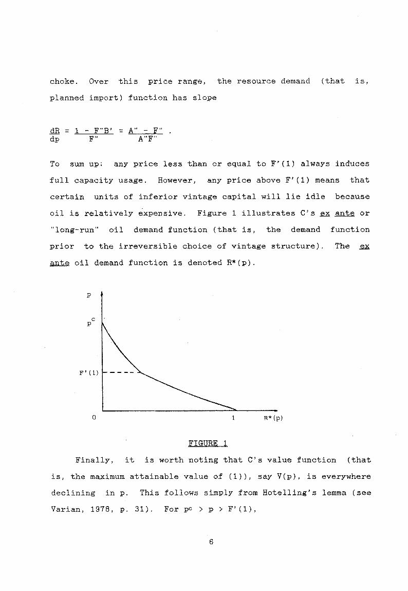
choke. Over this price range, the resource demand (that is,

planned import) function has slope

To sum up: any price less than or equal to F ' I I ) always induces

f u l l capacity usage. However, any price above F'(1) means that

certain units of inferior vintage capital will lie idle because

oil is relatively expensive. Figure 1 illustrates C' s ex ante or

"long-run'' oil demand function (that is, the demand function

prior to the irreversible choice of vintage structure). The ex

ante oil demand function is denoted R * [ p ) .

1 R* (P )

FIGURE 1

Finally, it is worth noting that C ' s value function (that

is, the maximum attainable value o f (l)), say V(p>, is everywhere

declining in p. This follows simply from Hotelling's lemma (see

Varian, 1978, p. 31). For pc > p > F'(l),

= F’(A.+R*) { $6 + &* } - R* - p &* - A ’ ( & ) $6 dp dp dP dP

= - R * < 0

since at the optimal solution F’= p = A ’ . Further, for

0 < p A F’(l), R* = (1-i) and

4 { F(1) - p(1-A) - A ( & ) } = - (1-A) + [ p - A ’ ( & ) 3 $6 dP dP

- - - (1-A.) < 0

recalling that p = A ’ at the optimal solution. Thus V’(p) < 0, as

asserted. As is intuitive, C is unambiguously worse off the

higher the oil price.

3 . The Stackelberp Precommitment Eo uilibrium (SPE).

I begin by assuming that S has access to a device.

(enforceable long-term contracts, for example) that makes its

price announcement a credible one. In any case, the optimization

problem considered in this section characterizes S ’ s best move at

decision node (i). Conceptually, S gauges C’s response - in

accordance with the analysis of the preceding section - under

every conceivable price announcement that it could make, and

“leads” by choosing p to maximize the static profit function

( 7 ) a‘ = pR - X(R) , subject to

(8a) p = F’(B(p)+R) f o r F’(1) < p < pc

(8b) R = {l - B(p)} f o r 0 < p 5 F’(1)“

7

where the cost. function X ( . ) displays X'(R)>O, X"(R)>O. Note that

the optimization problem does not explicitly take an exhaustion

constraint into account. This implies that S considers its

reserves of oil to be "large", so that the user cost of the

resource is very low. Alternatively, the cost function X ( . ) may

be thought of as already incorporating the user cost of the

resource.3

In general, the solution to the optimization problem

described by (7) and (8) may lie on either segment of the demand

function. If the optimal price announcement exceeds F'(l), it

will satisfy (8a) and

( 9 ) R + { p - X'(R) }(A"-F") = 0. A"F"

If there is no solution that simultaneously satisfies (8a ) and

(9), then S ' s optimal price announcement lies on the other

segment of the ante demand curve and is no larger than F'(1).

In this case, the solution is given by (8b) and

A "

I shall use (9) and (10) again later. For the moment define the

profit function as

"(PI = PR*(P) - X(R*(p))

where R*(p) is the implicit solution to F'(B(p)+R) = p, F'(1) < p

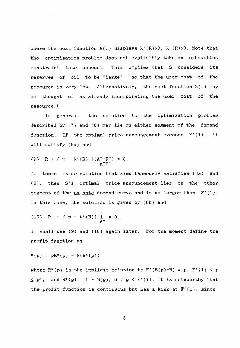
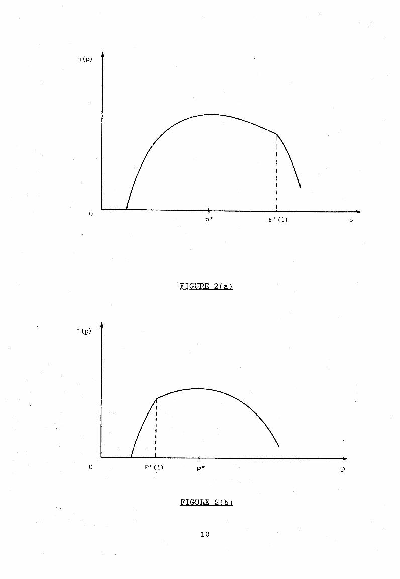
A per and R*(p) = 1 - B(p), 0 < p < F'(1). It is noteworthy that

the profit function is continuous but has a kink at F'(l), since

8

lim “(p) = lim *(PI - p+F’ (1 )+ p+F’(l)-

Figure 2 illustrates two possible shapes for the profit function.

Panel (a} depicts a case where the solution is given by (8b) and

( l o ) , and panel (b) a case where (8a) and ( 9 ) characterize the

solution. Naturally the second-order condition requires the

profit function to be concave at the maximum point. The maximum

point may also occur at the kink point.

At this point, it is easy to see that the SPE is not a

subgame perfect, or sequential, equilibrium. This is so because

once C is “locked in” with regard to its choice of technology

(that is, once C has irreversibly committed itself to a

particular value of 6 at decision node (ii)}, C ’ S elasticity of

demand for oil is lowered, and S typically has an incentive to

raise the price above the level originally announced. That this

is so will become apparent from the analysis in the sections that

follow. As a consequence, unless S is truly bound to abide by its

original price announcement (and C is truly confident thereof),

the

4.

SPE price is not a credible one.

The Cournot-Nash Eq uilibrium (CNE) or Stackelberw Sea uential Eauilibrium (SSE)

One interpretation of the optimization problem and solution

concept considered in this section is that C has already chosen

A and planned imports on the basis of S ’ s original price

announcement, but that S is now given the opportunity to revise

the price at which trade is to take place. That is, this section

characterizes S ’ s best move at decision node (iii). An

9

IT (PI

0

0

FIGURE 2(a )

FIGURE 2 ( b l

10

alternative interpretation of the current formulation is that, at

decision node (i), S behaves as a Cournot-Nash player in the

following sense: S forms a perfect forecast of C ’ s ex post demand

for the resource and announces an oil price to maximize profits,

given 6 . In other words, S emphatically fails to recognize the

effect of its price announcement on C ’ s choice of 6 .

In either case, S chooses p to maximize

( 7 ) pR - X(R) , subject now to

(lla) p = F’(L+R) for F’(1) < p < pc

(llb) R = (1-6) for 0 < p 5 F’(1)

treating A as given. It is immediately apparent that the optimal

price in this case will never be below F ’ ( 1 ) . This is because, if

f, is constant, the elasticity of demand is zero below a price of

F’(1); sales are invariant to price over this range, so S

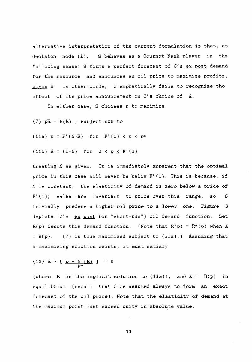
trivially prefers a higher oil price to a lower one. Figure 3

depicts C’s post (or “short-run”) oil demand function. Let

R(p) denote this demand function. (Note that R(p) = R*(p) when ii

= B(p). ( 7 ) is thus maximized subject to (lla).) Assuming that

a maximizing solution exists, it must satisfy

(12) R 3. I: p - X’(R1 3 = 0 F ”

(where R is the implicit solution to (lla)), and A = B(p) in

equilibrium (recall that C is assumed always to form an exact

forecast of the oil price). Note that the elasticity of demand at

the maximum point must exceed unity in absolute value.

0

FIGURE 3

It is worth stressing the point that in this model, the CNE

and the SSE are identical, Conceptually, the SSE differs from the

SPE only in that 5 has no recourse to a precommitment mechanism

in the former case. A s a result, the only credible price

announcement (equal by assumption to the price that C actually

forecasts) is that which S would choose once d had already been

irreversibly chosen. But this is precisely the premise on which

the derivation of the CNE price is based. In the absence of a

commitment mechanism, therefore, C correctly forecasts the CNE

price - regardless of S ’ s announcement - and chooses d

accordingly. Once 6 is (irreversibly) fixed, S ’ s optimal strategy

- is in fact to set the CNE price. The CNE is thus subgame perfect,

and C’s forecast is realized, as required.

5 . A Comparison of the SPE and the CNE

In this section I show that under certain fairly weak

conditions, the CNE oil price (pN) exceeds the SPE price ( p * > . If

this is the case, both C and S are easily shown to be worse off

in the CNE than in the SPE. That is, the CNE is P a r e t o inferior

to the SPE. However, even in cases where p N and p* cannot be

1 2

unambiguously ranked, it can still be demonstrated very simply

that the CNE is Pareto inefficient.

I begin by discussing the conditions required for p N to

exceed p*. Note first that if the SPE price is given by the

simultaneous solution of (10) and (8b), then it is trivially the

case that p* < pN. Next, suppose that the SPE is given by (9) and

(8a). Recall that for an interior solution F'(1) < pN < pc, the

CNE price is given by

(Recall that R(pN) is the implicit solution to (lla), for A, fixed

at the value B ( p N ) . ) Now because for F'(1) < p < p e r

it follows that

Thus f ' ( p ) < 0 at (and, by continuity, in a neighbourhood of) p N .

A minimal sufficiency condition for p N > p* would therefore

appear to be that ' f ' (p) 2 0, F'(1) < p < p*. A stranger

sufficiency condition is that s " ( p ) 4 0, F'(1) < p < p*; that is,

that the profit function is concave between the kink point and

its maximum point. To the right of the kink point, the profit

function has slope

13

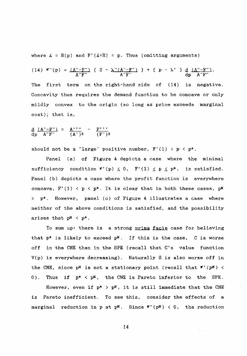
where L = B(p) and F'(L+R) = p. Thus (omitting arguments)

The first term on the right-hand side of (14) is negative.

Concavity thus requires the demand function to be concave cm only

mildly convex to the origin ( s o long as price exceeds marginal

cost); that is,

should not be a "large" positive number, F' (I) < p < p*.

Panel (a) of Figure 4 depicts a case where the minimal

sufficiency condition f ' ( p ) IO, F'(1) I p I p*, is satisfied.

Panel (b) depicts a case where the profit function is everywhere

concave, F'(1) < p < p*. It is clear that in both these cases, pN

> p*. However, panel (c) of Figure 4 illustrates a case where

neither of the above conditions is satisfied, and the possibility

arises that pN < p*.

To sum up: there is a strong prima facie case for believing

that p* is likely to exceed pN. If this is the case, C is worse

off in the CNE than in the SPE (recall that C's value function

V(p) is everywhere decreasing). Naturally S is also worse off in

the CNE, since pN is not a stationary point (recall that f'(pN) <

0 ) . Thus if p* < pN, the CNE is Pareto inferior to the SPE.

However, even if p* > pw, it is still immediate that the CNE

is Pareto inefficient. To see this, consider the effects of a

marginal reduction in p at pN. Since $ ' ( p N ) < 0 , the reduction

14

0 P

FIGURE 4(b)

0

FIGURE 4 t Cl

1 5

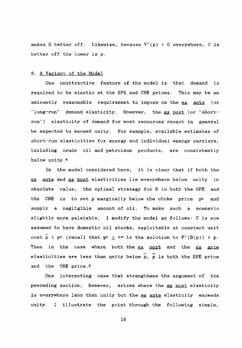
makes S better off. Likewise, because V'(p) < 0 everywhere, C is

better off the lower is p.

6 . A Variant of the Model

One unattractive feature of the model is that demand is

required to be elastic at the SPE and CNE prices. This may be an

eminently reasonable requirement to impose on the a ante (or

"long-run'' demand elasticity. However, the post (or "short-

run") elasticity of demand f o r most resources cannot in general

be expected to exceed unity. For example, available estimates of

short-run elasticities for energy and individual energy carriers,

including crude oil and petroleum products, are consistently

below unity. 4

In the model considered here, it is clear that if both the

ex ante and ex post elasticities lie everywhere below unity in

absolute value, the optimal strategy for S in both the SPE and

the CNE is to set p marginally below the choke price pc and

supply a negligible amount of oil. To make such a scenario

slightly more palatable, I modify the model as follows: C is now

assumed to have domestic oil stocks, exploitable at constant unit

cost < p" (recall that pc 5 +* is the solution to F'(B(p)) = p.

Then in the case where both the ex post and the ex ante

elasticities are less than unity below p , p is both the SPE price

and the CNE price.5

- -

One interesting case that strengthens the argument of the

preceding section, however, arises where the ex post elasticity

is everywhere less than unity but the ante elasticity exceeds

unity. I illustrate the point through the following simple,

16

though extreme, example.

FxamPle. Assume, contrary to what is postulated in (A.l),

that C has a fixed coefficients technology, such that.

manufacturing output is proportional to utilized capital. Thus

F(L+R) = B(b+R), B > 0. From (51, it is immediate that p < B

implies R = (1-A). Now suppose that p < a . Then so long as S

sets the price at (strictly, marginally below) or below p , C

-

imports (1-6) units of oil. It then follows from this that

CNE always features S setting the ceiling price p. This

because the CNE price is calculated on the premise that 6

- the

is

is

exogenously given; S ’ s perception in the CNE is therefore that

demand is completely inelastic up to p. By analogous reasoning,

it is easily checked that the SSE price is also the ceiling price

P. -

Consider now the SPE. For any price below p, R* = (1-6) , and

the elasticity of demand is given by

(recall that p = A ’ ( 6 ) , 0 < 6 < 1). I shall suppose that h(1;) =

31 < -1. A functional form with the required property is

where P > 0 is a constant. Note that

A ’ ( 0 ) = @ ( - 3 1 ) 1 i n 3 0 and lim A’(b) = +Q. &+l

Equating (15) with p yields, for & > 0,

17

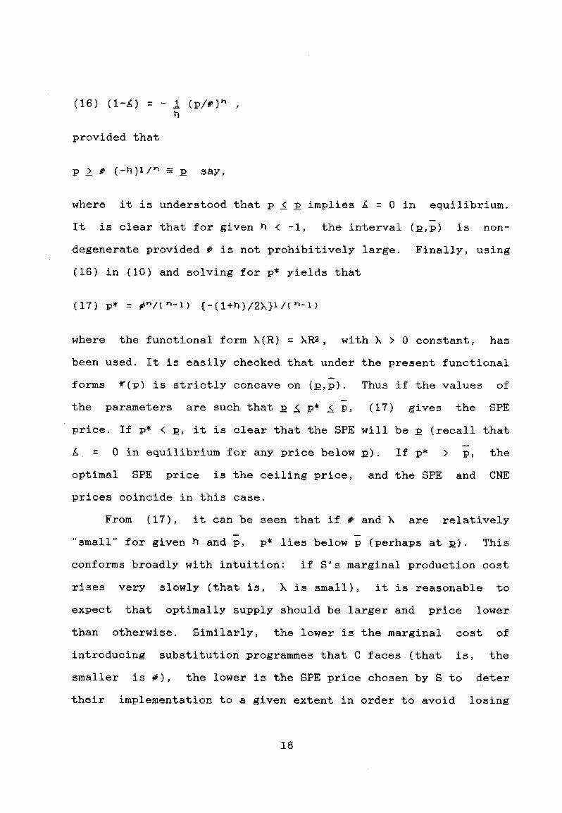
provided that

where it is understood that p A E implies d = 0 in equilibrium.

It is clear that for given l-1 < -1, the interval ( ~ , p ) is non-

degenerate provided @ is not prohibitively large. Finally, using

(16) in (10) and solving for p* yields that

-

where the functional form X ( R ) = XR2, with X > 0 constant, has

been used. It is easily checked that under the present functional

forms *(p) is strictly concave on (E,;). Thus if the values of

the parameters are such that E 5 p* 2 p , (17) gives the SPE

price. If p* < E, it is clear that the SPE will be E (recall that

d = 0 in equilibrium f o r any price below E). If p* > p, the

optimal SPE price is the ceiling price, and the SPE and CNE

prices coincide in this case.

-

From (17), it can be seen that if @ and X are relatively

"small" for given Is and p, p* lies below (perhaps at E). This

conforms broadly with intuition: if S ' s marginal production cost

rises very slowly (that is, X is small), it is reasonable to

expect that optimally supply should be larger and price lower

than otherwise. Similarly, the lower is the marginal cost of

introducing substitution programmes that C faces (that is, the

smaller is P ) , the lower is the SPE price chosen by S to deter

their implementation to a given extent in order to avoid losing

-

18

sales of oil. In sum, provided that S ' s marginal production cost

and the marginal cost of implementing substitution and resource-

saving programmes are sufficiently small relative to the unit

cost of domestic oil production in C, the SPE price lies below

the CNE price. Following the argument in the preceding section,

the absence of a precommitment mechanism in this case results in

an equilibrium that is Pareto-inferior to the SPE.

7. Concluding Remarks

This essay has elucidated one aspect of the rudiments of

Consumer-Producer relationships in the World Oil Market. Although

the construct I have used is overly simplistic, I have tried to

capture the mechanics of pre-emptive strategies by oil users and

long-term pricing considerations by producers. In particular, I

have sought to demonstrate in this context that credible

strategies sustain Pareto-inefficient equilibria. It has also

been shown under fairly weak conditions that the absence of long-

term agreements results in equilibria that are Pareto-inferior to

the equilibria when such agreements do obtain. If one gives the

result a slightly different interpretation, it may appear

somewhat counterintuitive that under precommitment more

"aggressive" leadership behaviour by the producer bloc

(Stackelberg versus Cournot behaviour) should typically benefit

the consumer bloc as well as the producer bloc.

This said, I have abstracted from a number of aspects that

are likely to be of importance. These include repercussions on

capital markets, feedback effects on oil demand due to the

maladjustment and adverse income effects following periods of

19

high oil prices (see Marquez, 1983, Chs. 2 and 5 for a

discussion). Perhaps most importantly, I have restricted the

analysis to what is essentially a two-period modely and thus

automatically excluded any possibility of "tacit cooperation"

between the producer and consumer blocs in the absence of binding

agreement mechanisms. In spite of these omissions, however, it

seems safe to conjecture that the principal results in this paper

would generalize.

20

Notes

1. I relax this in section 6 below.

2. Issues associated with strategic stockpiling or speculation are ignored here.

3. That is, the cost function imposes a penalty on current extraction that captures the value of having an extra unit of the resource still available for extraction once the game is finished. The drawback here is that players’ behaviour in any future game must be taken as given.

4. See Kouris (1983) for a survey. Geroski, Ulph and Ulph (1986) report estimates of short- and long-run demand elasticities for crude oil.

5. This is identical to the problem where a monopolist faces inelastic demand for a resource below a limit price (see Dasgupta and Heal, 1979, pp. 340-45).

2 1

References

Clifford, N. and V. P. Crawford (1987) "Short-term contracting and strategic oil reserves" Review of Economic Studies 54, pp. 311-323.

Dasgupta, P. S. and G. M. Heal (1979) Economic Theory and Exhaustible Resources, James Nisbet & Co., Welwyn, and Cambridge University Press, Cambridge.

Geroski, P. A. , A. M. Ulph and D. T. Ulph (1986) "A model of the crude oil market in which market conduct varies" Economic Journal 97, Supplement, pp. 77-86.

Kouris, G. (1983) "Energy demand elasticities in industrialized countries: a survey" The Enernv Journal 4, pp. 73-94.

Marquez, J. R. (1983) Oil Price Effec ts and OPE C's Pricing Policy, D. C. Heath and Company, Lexington, Massachusetts.

Newbery, D. M. G. (1981) "Oil prices, cartels, and the problem of dynamic inconsistency" Economic Journal 91, pp. 617-646.

Ulph, A. M. and G. M. Folie (1981) "Dominant firm models of resource depletion" in Currie, D., D. Peel and W. Peters (eds) Microeconomic Analysis: Essavs in Microeconomics and Development, Croom Helm, London.

Economic

Varian, H. R. (1978) Microeconomic Analvsia, W. W. Norton & Company, Inc., New York.

22

OXFORD INSTITUTE FOR ENERGY STUDIES 57 WOODSTOCK ROAD, OXFORD OX2 6FA ENGLAND

TELEPHONE (01 865) 31 1377 FAX (01865) 310527

E-ma i I: pub I ica tions@oxfo rde n e rg y . o rg http://www.oxfordenergy.org