effet tunnel et observation approchée pour des ...trelat/gdt/confs/camille_laurent... · effet...
TRANSCRIPT

Introduction Unique continuation and its quantification Hypoelliptic operators
Effet tunnel et observation approchée pour desopérateurs hypoelliptiques
Camille Laurent,CNRS, LJLL, Paris 6
avec Matthieu Léautaud, CMLS, Ecole Polytechnique
Groupe de travail Contrôle, LJLL, Paris 6, mai 2017

2/22
Introduction Unique continuation and its quantification Hypoelliptic operators
Degenerate hypoelliptic operators
We are interested in some class of degenerate operatorsLu = div(A(x)∇u) + b ·∇u with A(x)≥ 0
L =−m
∑i=1
X ∗i Xi (+X0).
where Xi are C∞ first-order differential operators.
Assumption (Hörmander hypothesis)There exists k ≥ 1 so that for any x ∈M ,Liek (X1, · · · ,Xm)(x) = Tx M .
This implies L hypoelliptic (Hörmander).

3/22
Introduction Unique continuation and its quantification Hypoelliptic operators
Question of approximate observability/controlability
We are interested in the quantification of the unique continuationproperty
u = 0 on ([0,T ]×)ω⇒ u = 0.
for some ω⊂M for some u solution of either
∂2t u−Lu = 0 wave like equation
⇓−Lu = λu eigenfunctions
∂tu−Lu = 0 heat like equation
Dual property : exact or approximate controlability

4/22
Introduction Unique continuation and its quantification Hypoelliptic operators
Introduction
Unique continuation and its quantification
Hypoelliptic operators

5/22
Introduction Unique continuation and its quantification Hypoelliptic operators
Classical Unique Continuation Theorems
Holmgren,John
• analyticcoefficients
• Φ noncharacteristic forP : p(x ,∇Φ) 6= 0
Tataru,Robbiano-Zuily,
Hörmander
• partially analyticcoefficients insome variable xa
• Φ pseudoconvexin ξa = 0
Carleman,Hörmander
• C∞ (even C1)coefficients
• Φ pseudoconvex :p,p,Φ> 0sufficient if realorder 2

6/22
Introduction Unique continuation and its quantification Hypoelliptic operators
Theorem (Tataru (95,99), with improvements by Robbiano-Zuily(98), Hörmander (97))Let x0 ∈ Rna×Rnb . P with smooth coefficients, analytic in the xa
variable. P analytically principally normal in ξa = 0 (OK if elliptic orreal invariant in xa).S = Φ = 0 oriented hypersurface pseudoconvex in ξa = 0.
If u solution of Pu = 0 near x0 and u = 0 in Φ≥ 0, then u = 0 in asmall neighborhood of x0.
The main tool is the Carleman estimate "with pseudodifferentialweight"
τ
∥∥∥e−ε
2τ|Da|2eτψu
∥∥∥2
m−1,τ≤ C
(∥∥∥e−ε
2τ|Da|2eτψPu
∥∥∥2
0+ e−τd ‖eτψu‖2
m−1,τ
)

7/22
Introduction Unique continuation and its quantification Hypoelliptic operators
Theorem (Quantification of the unique continuation with partialanalyticity)In the above geometric setting, P be a differential operator of order m,analytically principally normal operator on Ω in ξa = 0.Assume also that, for any ε ∈ [0,1 + η), the oriented surfacesSε = φε = 0 with φε(x ′,xn) := Gε(x ′)− xn are strictly pseudoconvexin ξa = 0 for P on the whole Sε.Then, for any open neighborhood ω⊂ Ω of S0, there are constantsκ,C,µ0 > 0 such that for all µ≥ µ0 and u ∈ C∞
0 (Rn), we have
‖u‖L2(K ) ≤ Ceκµ(‖u‖Hm−1
b (ω) +‖Pu‖L2(Ω)
)+
Cµm−1 ‖u‖Hm−1(Ω) ,
where we have denoted ‖u‖Hm−1b (ω) = ∑|β|≤m−1
∥∥∥Dβ
b u∥∥∥
L2(ω).

8/22
Introduction Unique continuation and its quantification Hypoelliptic operators
Theorem (Waves)Let M be a compact Riemannian manifold with boundary. Let ω be anon empty open subset of M , for any T > TUC = 2supx∈M d(x ,ω),there exist C,c > 0 such that for any (u0,u1) ∈ H1
0 (M )×L2(M ) andassociated solution u of
∂2t u−∆gu = 0 in [0,T ]×M ,
u|∂M = 0 in [0,T ]×∂M ,
(u,∂tu)|t=0 = (u0,u1) in M ,
(1)
we have,
‖(u0,u1)‖H1×L2 ≤ CecΛ ‖u‖L2(]0,T [×ω)
with Λ =‖(u0,u1)‖H1×L2
‖(u0,u1)‖L2×H−1the typical frequency of the solution.
Previous results : Lebeau (92) analytique case, Robbiano (95), Phung(02). See also Bosi-Lassas-Kurylev (16)

9/22
Introduction Unique continuation and its quantification Hypoelliptic operators
Approximate controllability for the wave
Theorem (Cost of boundary approximate control)For any T > TUC , there exist C,c > 0 such that for any ε > 0 and any(u0,u1) ∈ H1
0 (M )×L2(M ), there exists g ∈ L2((0,T )×ω) with
‖g‖L2((0,T )×ω) ≤ Cecε ‖(u0,u1)‖H1
0 (M )×L2(M ) ,
such that the solution of(∂2
t −∆)u = g in (0,T )×M ,(u,∂tu)|t=0 = (u0,u1), in M ,
satisfies∥∥(u,∂tu)|t=T
∥∥L2(M )×H−1(M )
≤ ε‖(u0,u1)‖H10 (M )×L2(M ).

10/22
Introduction Unique continuation and its quantification Hypoelliptic operators
Up to now, we will make the following assumptions :
M is a compact manifold without boundary (except in Grushin typecase)
L =−m
∑i=1
X ∗i Xi .
AssumptionThe manifold M , the density ds, and the vector fields Xi arereal-analytic.
k is the same as in Hörmander hypothesis.

11/22
Introduction Unique continuation and its quantification Hypoelliptic operators
General estimates for the wave
TheoremAssume that ω is a non empty open set of M and letT > supx∈M dL (x ,ω). Then, there exist C > 0 such that we have
‖(u0,u1)‖H 1L×L2 ≤ CecΛk ‖u‖L2(]−T ,T [×ω) , with Λ =
‖(u0,u1)‖H 1L×L2
‖(u0,u1)‖L2×H −1L
,
for any (u0,u1) ∈H 1L ×L2, and associated solution u solution
(∂2t −L)u = 1ωg in (0,T )×M ,
(u,∂tu)|t=0 = (u0,u1), in M ,
dL is the natural distance induced by the sub-Riemannian structurecoming from the control problem

12/22
Introduction Unique continuation and its quantification Hypoelliptic operators
Eigenfunction tunneling
TheoremLet ω be a nonempty open subset of M . Then, there is C,c > 0 suchthat every eigenfunction ϕi of L associated to the eigenvalue λi
satisfies
‖ϕj‖L2(M ) ≤ Cecλk/2j ‖ϕj‖L2(ω).
Optimal for the example of Grushin type (seeBeauchard-Cannarsa-Guglielmi (14) ).
Proof : Theorem on the wave easily implies eigenfunction tunnelingwith the solution u(t,x) = cos(
√λj t)ϕj .

13/22
Introduction Unique continuation and its quantification Hypoelliptic operators
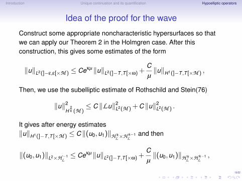
Idea of the proof for the wave
Construct some appropriate noncharacteristic hypersurfaces so thatwe can apply our Theorem 2 in the Holmgren case. After thisconstruction, this gives some estimates of the form
‖u‖L2(]−ε,ε[×M ) ≤ Ceκµ ‖u‖L2(]−T ,T [×ω) +Cµ‖u‖H1(]−T ,T [×M ) ,
Then, we use the subelliptic estimate of Rothschild and Stein(76)
‖u‖2
H2k (M )
≤ C ‖Lu‖2L2(M ) + C ‖u‖2
L2(M ) .
It gives after energy estimates‖u‖H1(]−T ,T [×M ) ≤ C ‖(u0,u1)‖H k
L×H k−1L
and then
‖(u0,u1)‖L2×H −1L≤ Ceκµ ‖u‖L2(]−T ,T [×ω) +
Cµ‖(u0,u1)‖H k
L×H k−1L
,

13/22
Introduction Unique continuation and its quantification Hypoelliptic operators
Idea of the proof for the wave
Construct some appropriate noncharacteristic hypersurfaces so thatwe can apply our Theorem 2 in the Holmgren case. After thisconstruction, this gives some estimates of the form
‖u‖L2(]−ε,ε[×M ) ≤ Ceκµ ‖u‖L2(]−T ,T [×ω) +Cµ‖u‖H1(]−T ,T [×M ) ,
Then, we use the subelliptic estimate of Rothschild and Stein(76)
‖u‖2
H2k (M )
≤ C ‖Lu‖2L2(M ) + C ‖u‖2
L2(M ) .
It gives after energy estimates‖u‖H1(]−T ,T [×M ) ≤ C ‖(u0,u1)‖H k
L×H k−1L
and then
‖(u0,u1)‖L2×H −1L≤ Ceκµ ‖u‖L2(]−T ,T [×ω) +
Cµ‖(u0,u1)‖H k
L×H k−1L
,

14/22
Introduction Unique continuation and its quantification Hypoelliptic operators
Previous results on hypoelliptic operators : uniquecontinuation
• positive results : Bony (69) using Holmgren, Garofalo (93)Grushin like operators...
• negative results : Bahouri (86) large class of counterexamples forL + V with L like Heisenberg...

15/22
Introduction Unique continuation and its quantification Hypoelliptic operators
Previous results of control of hypoelliptic heat-like operators
• Type I (X0 = 0) : Grushin (see after)Beauchard-Cannarsa-Guglielmi (14), Beauchard-Miller-Morancey(15), Koenig (17)Heisenberg : Beauchard-Cannarsa (17)
• Type II : Kolmogorov : Beauchard-Zuazua (09), LeRousseau-Moyano (16), Beauchard-Helffer-Henry-Robbiano (15)Ornstein-Uhlenbeck operators : Beauchard-Pravda-Starov (16)

16/22
Introduction Unique continuation and its quantification Hypoelliptic operators
General estimates for the heatTheoremFor all T > 0, there exist C,c > 0 such that for any u0 ∈H 1
L andassociated solution u of ∂tu−Lu = 0, we have
‖u0‖2L2 ≤ CecΛk
∫ T
0
∫ω
|u(t,x)|2 dx dt, Λ =‖u0‖H 1
L
‖u0‖L2, (2)
Elliptic case : Fernandez-Cara-Zuazua (00), Phung (04)
Corollary (Exponential cost of approximate null control)For any T > 0, there exist C,c > 0 such that for any ε > 0 and anyu0 ∈ L2(M ),u1 ∈ L2(M ), there exists g ∈ L2((0,T )×ω) with
‖g‖L2((0,T )×ω) ≤ Cec
εk∥∥e−T L u0−u1
∥∥L2(M )
,
such that the solution of ∂tu−Lu = g issued from u0 satisfies
‖u(T )−u1‖H −1L≤ ε∥∥e−T L u0−u1
∥∥L2(M )
.

17/22
Introduction Unique continuation and its quantification Hypoelliptic operators
Previous results on heat-like Grushin type operators
‖u(T )‖2L2(M ) ≤ C
∫ T
0
∫ω
|u(t,x)|2 dtdx , u solution of heat (3)
Theorem (Beauchard, Cannarsa and Guglielmi (14))Assume L = ∂2
x + x2γ∂2y with Dirichlet on [−1,1]x × [0,1]y .
1. If γ ∈ [0,1[, then the observability inequality (3) holds true for anynonempty open set ω⊂M in any time T > 0.
2. If γ = 1 and if ω =]a,b[×]0,1[ where 0 < a < b < 1, then thereexists T ∗ ≥ a2/2 such that
• for every T > T ∗ the observability inequality (3) holds true,• for every T < T ∗ the observability inequality (3) is false.
3. If γ > 1 and ω⊂ (0,1)× (0,1), then (3) is false, in any T > 0.
Theorem (Koenig (17))γ = 1. Assume that there is 0 < c < d < 1 such thatω∩
(]−1,1[×]c,d [
)= /0. Then, for any T > 0, (3) is false.

18/22
Introduction Unique continuation and its quantification Hypoelliptic operators
The specific case k = 2
TheoremAssume that k = 2. There exist T ∗ > 0 such that for all T > T ∗ and allε > 0, we have for any solution u to ∂tu−Lu = 0,
‖u(T )‖2L2 ≤
1
εβ
∫ T
0
∫ω
|u(t,x)|2 dt dx + ε‖u(0)‖2L2 . (4)
Corollary (Polynomial cost of approximate null control if k = 2)For any u0 ∈ L2, there exists g ∈ L2((0,T )×ω) with
‖g‖L2((0,T )×ω) ≤C
εβ‖u0‖L2 ,
such that the associated solution u of ∂tu−Lu = g satisfies
‖u(T )‖L2(M ) ≤ ε‖u0‖L2 ,

19/22
Introduction Unique continuation and its quantification Hypoelliptic operators
Structure of the proof
Theorem on the wave implies Theorem on the heat using some variantof the transmutation method as done by Ervedoza-Zuazua (11) :There exists some kernel kT (t,s) compactly supported in t such that ify is solution of the heat, u(s) =
∫ T0 kT (t,s)y(t)dt is solution of the
wave.
The case k = 2 is the limit case where the cost of the control≈ ecλk/2
= ecλ is of the same order of the dissipation e−λT of the heat.That is why we need T large to get a polynomial cost.Lebeau-Robbiano in one shot.

20/22
Introduction Unique continuation and its quantification Hypoelliptic operators
Some "Lebeau-Robbiano like" estimates
LemmaThere exist C,γ > 0 such that for any T > 0,λ≥ 0, for every y0 ∈ Eλ
and associated solution y to ∂ty−Ly = 0, we have
‖y(T )‖2L2 ≤
CT
e(2γλk/2+ CT )
∫ T
0
∫ω
|y(t,x)|2 dt dx .
Rk : k = 1 : elliptic Lebeau-Robbiano, k = 2 (Grushin) behaves likehalf-Laplacian

21/22
Introduction Unique continuation and its quantification Hypoelliptic operators
Further resultats we have obtained
• polynomial cost in some Gevrey type spaces
• some Grushin type cases where we only need partial analyticity(with respect to y only) and allow a boundary
• Λ =‖(u0,u1)‖H 1
L×L2
‖(u0,u1)‖L2×H−1
L
may be changed by Λ1/ss with
Λs =‖(u0,u1)‖H s
L×H s−1L
‖(u0,u1)‖L2×H−1
L
for any s > 0
Further open problems
• in the case k = 2, find the right condition to get from exactcontrollability to approximate controlability with polynomial cost
• understand more generally the case when drift X0 is necessary

22/22
Introduction Unique continuation and its quantification Hypoelliptic operators
MERCI DE VOTRE ATTENTION! ! ! ! !