effects of water priority policy on farmers’ decision on...

1

Effects of water priority policy on farmers’ decision 1

on acreage allocation in northwest China 2

Lei Zhang1,2* and Thomas Herzfeld3 3

1 Development Economics Group, Wageningen University, The Netherlands 4 2 China Centre for Land Policy Research, Nanjing Agricultural University, P.R. China 5 3 Department Agricultural Policy, Leibniz-Institute of Agricultural Development in 6

Central and Eastern Europe, Germany 7

* Corresponding author. Email: [email protected] 8

9

Abstract: 10

This article analyses the impact of a water allocation priority policy for a specific crop 11

on farmers’ acreage allocation to different crops. To accomplish this, a system of crop 12

acreage demands conditional on output yields, prices of variable inputs and levels of 13

quasi-fixed inputs is estimated. The analysis based on a two-year farm household 14

panel data from an arid region in northwest China. The results show that the water 15

policy change results in a lower elasticity of land demand not only for Atlantic 16

potatoes (i.e. the preferential crop), but also for the other crops. Acreage allocation to 17

grains differs from other crops due to their use within the farm household. Moreover, 18

the estimated elasticities of quasi-fixed inputs reveal that whereas the area of cash 19

crops and Atlantic potatoes increases with increased use of own labour before the 20

policy change, it does so only for cash crops after the policy change. With respect to 21

own and exchanged labour Atlantic potatoes behave like grains and regular potatoes 22

after the policy change. 23

Key words: water scarcity, priority allocation, agricultural production 24

25

26

2

1. Introduction 27

Governments interfere quite often in producer’s decision space in agricultural 28

production systems. In this context the access to irrigation water is contested in many 29

countries, the more water becomes a scarce input. For this and other reasons, 30

governments regulate the access to irrigation water. The effects of such interferences, 31

especially related to water entitlements or water prices, have been frequently analysed 32

for agricultural systems in North America and Europe (Coyle, 1993; Gorddard, 2009; 33

Villezca-Becerra and Shumway, 1992; Moore and Negri, 1992; Fezzi and Bateman, 2009). 34

However, few analyses are known for countries undergoing a process of economic 35

and institutional transformation where property rights might be less clearly defined. 36

Furthermore, often implementation and the working of enforcement mechanisms 37

differ from what is known in North America and Europe. 38

Agricultural economists often have favoured modelling crop production decisions 39

in terms of acreage responses rather than output supplies (Coyle, 1993). The key 40

argument is that acreage planted is essentially independent of many non-behavioural 41

factors such as seed quality, harvesting intensity and weather conditions, and hence 42

may provide a closer proxy to planned production than does observed output (Coyle, 43

1993; Arnade and Kelch, 2007). 44

Most previous area response studies have estimated response functions separately 45

for individual crops using a Nerlovian framework of partial adjustment and adaptive 46

expectations (Nerlove, 1956; Askari and Cummings, 1977). However, problems in 47

econometric specification and estimation of Nerlove models have been widely 48

discussed and a number of papers extend the Nerlove model or other acreage response 49

models to a system of multiple crops. Krakar and Paddock (1985) and Bewley, et al. 50

(1987) use a multinominal logit approach in studying the allocation of fixed resources 51

between alternative uses. Coyle (1993) developed an econometric model of crop 52

acreage demands (for Western Canada) conditional on total crop acreage and related 53

separability and dynamic specifications to reduce the effects of multicollinearity in 54

the system. Hussain et al. (1999) estimate changes in crop areas in response to 55

changes in output prices in Australian broad-acre agriculture, based on a model as a 56

set of acreage allocation decisions made simultaneously but at a number of 57

hierarchical stages. More recently, Gorddard (2009) estimates an econometric model 58

3

of Saskatchewan crop land-allocation behaviour and tests for joint production in the 59

presence of a land constraint. 60

There are several studies investigating the effects of subsidies and pricing policies 61

related to agricultural production on crop allocations (Zavaleta, 1987; Rosegrant et al., 62

1995) or water entitlements on producer behaviour (Moore and Negri, 1992). 63

Nevertheless, the impact of water policies favouring selected crops and the policy’s 64

effect on acreage allocation to different crops has rarely been analysed. Land is 65

always regarded as the most fundamental input in agricultural production. However, 66

for the production of water-intensive crops in arid regions, land without irrigation 67

water is almost valueless. 68

In this paper, we present a model estimating the interaction of the two crucial 69

inputs in the agricultural production system: land and water. Specifically, we analyse 70

the impact of a water allocation priority policy for a specific potato variety on 71

farmers’ decision on acreage allocation among crops. We use the case of an arid 72

region in northwest China, where agricultural is the biggest consumer of water taking 73

88.1% of total water resources.1 The policy change regarding water allocation has 74

been caused by the entry of a potato processor in this region which is partly owned by 75

the regional government. The potato processing company entered in 2008 and 76

demands a specific variety of potatoes, called Atlantic potatoes, for processing into 77

flakes and starch. In order to meet the growing demand for Atlantic potatoes, the local 78

government assigned water allocation priority for Atlantic potato growing to stimulate 79

its production in this area. The water allocation priority policy requires that in spite of 80

the water scarcity in this region, a sufficient amount of irrigation water (i.e. the 81

amount of water that is physically required for a crop’s production) has to be reserved 82

for irrigating Atlantic potatoes. The remaining quantity of irrigation water is then 83

allocated among the other crops. However, the stimulation of producing a crop with 84

relatively high water demands via institutional instruments conflicts with the 85

insufficiency of irrigation water in northwest China. Moreover, the sensitivity to pests 86

and diseases imposes other technical restrictions on potato production (Franke et al., 87

2011). All these factors raised concerns about the water allocation priority policy. 88

1 Water Management Bureau of Minle County, Gansu Province, P.R. China (2007).

4

This study aims to analyse the effect of the water allocation priority policy on 89

farmers’ production decisions. We estimate the reaction of farmers to the introduction 90

of the priority policy in their acreage allocation to various crops. The analysis uses a 91

unique two-year panel data set of farmers’ acreage decisions. This article contributes 92

to the literature by analyzing the impact of a priority policy for one agricultural input 93

used for a specific crop. Compared to standard partial equilibrium analyses, our study 94

covers the whole cropping part of the farm household and includes indirect effects of 95

the water priority policy on other crops than Atlantic potatoes. 96

The remainder of this article is organized as follows. The following section 97

establishes, based on a theoretical framework, a set of conditional land demand 98

functions which will be estimated econometrically. Next, we describe the study area 99

and the data underlying the econometric analysis. Subsequently, in section 4, we 100

present and discuss the econometric results. The final section summarizes the main 101

results of the empirical analysis and provides some policy recommendations. 102

103

2. Conceptual framework 104

Farmer’s decision of allocating total land to various crops can be modelled 105

basically in three different ways (Arnberg and Hansen, 2012; Moore et al., 1994). 106

Programming models, for instance used by Amir and Fisher (2000) to evaluate water 107

policies in Israel, unfortunately, lack a theory-based behavioural model. Among the 108

approaches based on neoclassical producer theory, two strands can be distinguished. 109

Models assuming input jointness assign inputs to all crops. Such an approach does not 110

allow for a specific analysis of substitution in input use between crops. Alternatively, 111

Moore et al. (1994) assign all inputs except one quasi-fixed but allocatable input (e.g. 112

land) to individual crops. That is, variable inputs are used non-joint. The latter 113

approach has the advantage that interdependences across crops can be accounted for 114

explicitly in the model. Here we follow the non-jointness approach. 115

Each farmer is assumed to behave rationally and risk-neutral. Initially each 116

farmer has a fixed amount of irrigation water which can be allocated to the various 117

crops. Water trade is permitted since 2002 in this area. However, the vast majority of 118

farmers do not engage in. Accordingly, each farmer decides how much land to assign 119

to the different crops based on an optimisation procedure. Here, we assume the farmer 120

to minimise costs of producing a given level of outputs. 121

5

Assume a farmer operates in a near optimal situation before the introduction of 122

the water priority policy. After the policy change, the farmer looks for a new optimal 123

input allocation by minimising costs subject to the previous level of output. Thus, the 124

intermediate-run decision is the choice of the crops to grow and their acreage. All 125

crops relevant for our analysis have been assigned to four groups: grain crops, cash 126

crops, regular potatoes and Atlantic potatoes. Contrary to other studies, e.g. Moore et 127

al. (1994), the land allocation is variable. The resulting first-order conditions state that 128

each input’s value of the marginal product in each use should be equal to the 129

respective input’s price. Introducing a priority policy for one crop, here Atlantic 130

potatoes, implies an indirect subsidy of the input water for a specific use and an 131

indirect taxation of this input in alternative uses. To quantify this effect we analyse the 132

allocation of land to the different outputs. That is, based on the optimisation, the 133

farmer decides how much land to allocate to output yj. The resulting conditional input 134

demand function for land xAj is a function of output yields, prices of variable inputs 135

(w) and levels of quasi-fixed inputs (z): 136

xAj = f(yj, w, z); for j = 1, ..., n 137

Dividing each equation by total area (xA) returns conditional land demand as a 138

system of land share equations and normalised exogenous variables: 139

sj = xAj/x

A = f(yj*, w*, z*); for j = 1, ..., n. 140

Choosing a flexible approximation to a set of possible functional forms, we are 141

left with the quadratic and translog functional form. Due to zero observations for 142

outputs and inputs a quadratic functional form seems the best choice. Therefore, the 143

conditional input demand function derived from a quadratic cost function is: 144

sj = β0 + Σk βΑk w*k + βAj y

*j + Σt βAt z

*t; for j = 1, ..., n.. 145

Together the share functions represent a system of conditional demand functions. 146

Therefore, the standard theoretical restrictions will apply: The crop specific constants 147

should add up to unity, the cross-terms should be symmetric and the functions should 148

be homogeneous of degree zero in prices. 149

We are especially interested in the effect of the water policy’s change on the 150

acreage allocation across outputs. It is expected that farmers increase the share of land 151

allocated to Atlantic potatoes produced for the manufacturer resulting in a lower 152

6

elasticity of land demand. All other crops are expected to show an increasing elasticity 153

of land demand with respect to the price of water. 154

155

3. Research area and data collection 156

For this research, we use data that we collected via two surveys held in Minle 157

County, Zhangye City, Gansu Province. These surveys were carried out in May 2008 158

and May 2010. The 2008 survey serves as a baseline survey to assess the situation 159

before the entry of the potato processing company in Minle County and the related 160

water policy change. The 2010 survey is used to assess the impact of the new water 161

policy on farmers’ decisions on acreage allocation among crops. 162

Zhangye City is an oasis located midstream of the Heihe River, an inland river 163

that flows across Qinghai Province, Gansu Province and Inner Mongolia Autonomous 164

Region. It originates from the Qilianshan Mountains in Qinghai province and ends in 165

Juyanhai Lake in Inner Mongolia. In the midstream of the Heihe River watershed, the 166

land is flat, sunshine is abundant, and annual precipitation is very low while the 167

evaporation is high. But due to the availability of irrigation water from the Heihe 168

River, the area has become a major grain and vegetables production base in Gansu 169

province. 170

According to the MWR2 (2004), Zhangye City is severely short of water 171

resources, even though it uses up almost all the water of Heihe River. Only 50% of 172

farmland is well irrigated, and much arable land has been abandoned due to water 173

shortage. Agriculture accounts for approximately 95% of all water use and almost all 174

water in the Heihe River is extracted for irrigation use. As a result, too little water 175

flows into Juyanhai Lake, which dried out in 1992 and an area of 200 km2 around the 176

lake became desert (MWR, 2004; Zhang et al., 2009). 177

To deal with these problems, the Ministry of Water Resources initiated a pilot 178

project called ‘Building a Water-saving Society in Zhangye City’ in 2002. This project, 179

which is the first of its type in the country, was designed to save water through 180

government investments in a water-saving irrigation system and in meters for water 181

users and through establishing a system of water use rights (WUR) with tradable 182

2 Ministry of Water Resources

7

water quotas. The first two measures decreased irrigation water use somewhat, but 183

trading of WUR did not become popular (Zhang et al., 2009). 184

Minle County, one of the six counties in Zhangye City, is located between the 185

foothills of the Qilian Mountains and the lower lying Hexi corridor. Its total cultivated 186

land area equals 860,000 mu3, with irrigated land constituting 67 %. Major crops in 187

Minle County include barley, wheat, maize, sesame, rapeseed, garlic and potato. As 188

rotation, farmers in Minle County regularly change plots devoted to different crops. 189

Surface water is the major water resource for irrigated agriculture in the area. Due to 190

the high costs of pumping water from the wells, the use of groundwater is less than 191

5 % of total water use in irrigated agriculture (Water Bureau of Minle County). 192

Agricultural land in Minle County is usually divided into three zones with 193

different planting conditions and water requirements. Zone 1 has an elevation ranging 194

from 1,600 to 2,000 meters. Precipitation in this zone is relatively scarce. Zone 2 is 195

located between 2,000 and 2,200 meters, while Zone 3 has an elevation ranging from 196

2,200 to 2,600 meters. By far the largest zone is the second one, with 500,000 mu of 197

cultivated land, followed by the first and third zones, with 190,000 and 170,000 mu 198

respectively. Agricultural production in the first and second zones generally uses 199

irrigation, while most agricultural production in the third zone is rain fed. 200

The water used for surface irrigation is stored in seven reservoirs in the 201

Qilianshan Mountains. Each of these reservoirs serves its own irrigation area within 202

Minle County. A county-level water management bureau (WMB) is responsible for 203

the water allocation institutions within the region. Seven lower-level WMBs, one for 204

each of the seven irrigation areas, arrange the water allocations to WUAs within their 205

own irrigation area. WUAs are responsible for arranging the water allocation to 206

households belonging to their own WUA. The households within each WUA are 207

sub-divided into water user groups (WUGs), consisting of households having plots 208

along the same channel. Since the plots of different households within a WUG are 209

irrigated at the same time, households belonging to a WUG need to coordinate their 210

planting decisions and water demands. 211

Irrigation is carried out by flooding adjacent farmland at the same time, organized 212

from lowest to highest altitudes, with villages in the first zone receiving more 213

3 15 mu equals one hectare.

8

irrigation rounds (generally three) per year than the villages in the other two zones 214

(generally one or two rounds). Standard water quantities per mu are assigned for each 215

flooding, but these quantities are only realized in years of abundant rainfall. Water is 216

allocated according to a quota system based on the size of the so-called WUR land of 217

the farmers. Not all the irrigated land is classified as WUR land. Its size depends on 218

the amount of labour provided by a village to the construction of the reservoir and 219

other factors. 220

The household survey data used in this study were collected in May 2008 and 221

May 2010 by staff and students from Gansu Academy of Social Sciences in Lanzhou, 222

Gansu Agricultural University in Lanzhou, and Nanjing Agricultural University. The 223

data cover information over the years 2007 and 2009 containing information about 224

land use, crop production, use as well as prices of water and other inputs, WUA 225

participation and land tenure. Household interviews were done in the same 21 villages 226

were a similar household survey was held in May 2008 (see Wachong Castro et al., 227

2010 for a description of the sampling method). If possible, the same households in 228

each village that were interviewed in 2008 were also interviewed in May 2010. In 229

cases were the same household could not be found, it was replaced by another, 230

randomly selected, household in the same village. This resulted in a panel dataset 231

containing 265 households. Six households among them rented out their land to other 232

households and were engaged in off-farm work, thus didn’t grow any crops either in 233

2007 or in 2009. Additionally, households that had missing data on one or more 234

variables used in the empirical analysis and the outliers4 were excluded. Finally, the 235

following empirical analysis uses a two-year panel dataset containing 248 236

observations (households). 237

In order to simplify the econometric model, we aggregate crops into four groups: 238

grains (barley, wheat, sesame and maize), cash crops (rapeseed and garlic), Atlantic 239

potatoes supplied to the processing company and regular potatoes (various local 240

varieties). 241

242

4. Data analysis and results 243

4 Here we define outliers as households with large changes (>50%) in area shares of any crops between

the two years.

9

Total land per household remained almost constant between the two years.5 That 244

is, the introduction of the water priority policy had no effect on farmers’ decision to 245

remain in agriculture. However, the policy change in terms of water allocation is 246

expected to affect the acreage allocation decision. The possibly changing intensity of 247

other inputs’ use might be affected by the water priority policy. For instance, rational 248

behaviour suggests a reduced use of inputs when the marginal product decreases 249

given constant input and output prices. Therefore, in crop-specific production 250

functions, we apply area shares rather than absolute value of planting areas as the 251

dependent variable. 252

Table 1 displays average area shares of the four output categories in 2007 and 253

2009 (first two columns) and their changes from 2007 to 2009 (last columns). 254

Table 1 255

256

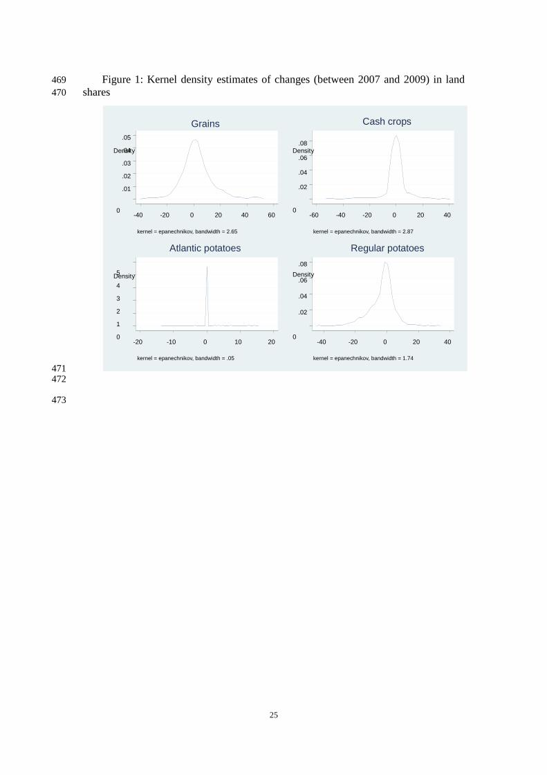
Because the table presents only changes in the mean and might underrepresent 257

changes in the tails of the distribution, Graph 1 displays the changes as Kernel 258

Density estimates. Obviously, the overwhelming majority of farmers kept area shares 259

rather constant. Cash crops and regular potatoes experienced on average a reduction. 260

The reduction in area share is particularly remarkable for regular potatoes, highly 261

probable due to an increase of the share of Atlantic potatoes. 262

Graph 1 263

264

In the following econometric model the acreage allocation will be explained by 265

output levels, prices of variable inputs6, levels of quasi-fixed inputs and factors 266

besides agricultural inputs (e.g. human capital, managerial capabilities, household 267

characteristics and farm characteristics). All equations include village dummies to 268

control for regional effects. The definition of all explanatory variables is presented in 269

Table 2. 270

5 The total areas of arable land for each household on average are 15.4 mu and 15.3 mu in 2007 and

2009, respectively. 6 There is little variation of prices of pesticide between the households. Therefore, we do not

incorporate the pesticide price in the models.

10

Table 2 271

272

The system of land share equations is estimated in two specifications. First, we 273

estimate two static systems for 2007 and 2009. Second, we estimate the system in first 274

differences. The first estimates can be interpreted as presenting farmers’ behaviour on 275

average before and after the water priority policy’s introduction. The second estimates 276

explore more the change at farm level, by taking out unobserved farm-specific effects 277

due to first differencing. Of course the second model will miss all time invariant 278

explanatory variables like farmer’s age as well as slope and fertility of land. 279

The following Table 3 presents the elasticities derived from the estimated 280

coefficients.7 The estimated coefficients are presented in the Appendix. 281

Table 3 282

283

The estimated elasticities indicate that crop-share responses to the changes in 284

variable input prices vary between different crops. Clearly, acreage allocation to 285

grains shows the least elastic response variable inputs’ prices and fixed inputs. 286

Similarly, output changes cause a more elastic change in land demand for grains. This 287

result holds for the model in levels and for both years. One reason for this behaviour 288

lies in the essential proportion of grains grown by farmers and the prominent role of 289

grains in peoples’ diet. Grains are not only planted for selling on markets, but also 290

used for own food consumption. That is, grains form the most important element in 291

farmer’s acreage allocation and will be substituted less against other crops. 292

Generally, elasticities of variable inputs are rather small. One remarkable 293

exception is the effect of water price changes in 2007 on acreage demand for cash 294

crops and Atlantic potatoes. Surprisingly, the estimated elasticities are positive, 295

indicating a larger allocation of land to cash crops and Atlantic potatoes in areas 296

where water prices are higher. Estimation without village controls yields much higher 297

7 The elasticities of the response of area shares of different crops to a change in prices of variable

inputs and levels of quasi-fixed inputs are calculated as: ii

i s

w βε *=

11

elasticities8. Therefore, regional variation in the water price across WUAs does not 298

fully explain the higher reagibility of acreage allocation to cash crops and Atlantic 299

potatoes with respect to water price compared to the other two categories. Area 300

devoted to regular potatoes is predicted to be smaller in areas with a higher water 301

price in the 2007 model. After the introduction of the water priority policy, estimated 302

elasticites with respect to water drop markedly across all crops. Differences across 303

crops disappear and all elasticities turn out to be positive but very small. Atlantic 304

potatoes become less attractive; the estimated elasticity drops to 0.021. On the other 305

hand, for regular potatoes the elasticity increases from -0.038 to 0.030 after the water 306

policy change. 307

Regarding the other variable inputs, hired labour stands out for the two types of 308

potatoes. Similarly, the price of seeds is predicted to cause a stronger reaction of 309

acreage allocation to cash crops and Atlantic potatoes compared to the two other two 310

crop categories. Surprisingly, the elasticity for Atlantic potatoes has a positive sign. 311

Turning to the quasi-fixed inputs reveals an interesting change of Atlantic 312

potatoes’ position. Whereas the area of cash crops and Atlantic potatoes increases with 313

increased use of own labour before the policy change, it does so only for cash crops 314

after the policy change. With respect to own and exchanged labour Atlantic potatoes 315

behave like grains and regular potatoes after the policy change. With respect to 316

machinery services there is no change in signs for Atlantic potatoes. 317

Consistent with theoretical expectations, the output elasticities are all positive. An 318

increase in crop yields leads to an increase in the area share for each of the four 319

categories of crops. For instance, in 2007, the area share of Atlantic potatoes is 320

predicted to increase by 0.006 %, when the yield of Atlantic potatoes goes up by 1 %. 321

After the introduction of the water priority policy, output elasticity becomes markedly 322

larger for both types of potatoes. 323

The results of model 2 show that farmers in areas were water prices increased 324

reduced their acreage allocation to cash crops, Atlantic potatoes and regular potatoes. 325

On the contrary, area devoted to grains increased. This is reasonable because grains 326

receive less amount of water compared to the other three categories of crops. 327

8 Detailed results available from the authors upon request.

12

Furthermore, increase in wages for hired labour affects cash crops most. The same 328

holds for the amount of own labour and machinery service. 329

330

5. Conclusions and policy recommendations 331

This article analyses the impact of a priority policy for one agricultural input used 332

for a specific crop on farmers’ acreage allocation to different crops. To accomplish 333

this, we estimate a system of crop acreage demands conditional on output yields, 334

prices of variable inputs and levels of quasi-fixed inputs. The analysis bases on a 335

two-year farm household panel data from an arid region in Northwest China. Previous 336

research on this subject has concentrated on the case studies in North America, where 337

property rights are relatively well-defined. Our research provides an example for 338

countries undergoing a process of economic and institutional transformation where 339

property rights might be less clearly defined. 340

Our findings indicate that policies related to water allocation regulation have 341

remarkable effects on farmers’ acreage allocation to various crops. More specifically, 342

elasticities calculated from the coefficients of the econometric models show that 343

before the introduction of the priority policy land demand is more elastic with respect 344

to the price of water, particularly for the preferential crop (i.e. Atlantic potatoes). The 345

elasticity effects of the prices of other variable inputs are relatively low. After the 346

priority policy was introduced, the acreage changes become less elastic to the changes 347

of water price. 348

The assumption of plots having no quality differences and to be fully divisible 349

poses a limitation to our conceptual framework. Adding crop rotation requirements is 350

straightforward and has been demonstrated by Arnberg and Hansen (2012). 351

An important policy implication that emerges from our results is that priority 352

policy for an agricultural input clearly affects factor allocation within households, 353

thus creates imbalances in remuneration of fixed factors. 354

355

13

References: 356

Amir, I., Fisher, F.M., 2000. "Response of Near-optimal Agricultural Production 357 to Water Policies". Agricultural Systems 64: 115-130. 358

Arnade, C., and Kelch, D., 2007. Estimation of area elasticities from a standard 359 profit function. American Journal of Agricultural Economics 89, 727-737. 360

Arnberg, S., Hansen, L.G., 2012. "Short-run and long-run dynamics of farm land 361 allocation: panel data evidence from Denmark". Agricultural Economics 43: 179-190. 362

Askari, H. and Cummings, J.T., 1977. Estimating agricultural supply response 363 with the Nerlove model: a survey, International Economic Review 18, 257-292. 364

Bewley, R., Young, T. and Colman, D., 1987. A system approach to modelling 365 supply equations in agriculture. Journal of Agricultural Economics 35, 151-166. 366

Coyle, B.T., 1993. On modelling systems of crop acreage demands. Journal of 367 Agricultural and Resource Economics 18, 57-69. 368

Fezzi, C. and Bateman, I.J., 2009. Structural agricultural land use modelling. The 369 27th International Conference of the International Association of Agricultural 370 Economists, Beijing, P.R. China. August 16-22, 2009. 371

Franke, A.C., Steyn, J.M., Ranger, K.S., and Haverkort, A.J., 2011. Developing 372 environmental principles, criteria, indicators and norms for potato production in South 373 Africa through field surveys and modelling. Agricultural Systems 104, 297-306. 374

Gorddard, R.J., 2009. Modeling profit-maximizing land-allocation behavior. 375 Agricultural and Resource Economics. Davis, University of California. Ph.D. 376

Hussain, I., Liaw, A. and Hafi, A., 1999. Modeling crop area allocations in 377 Australian broadacre agriculture. Combined 43rd Annual Australian and 6th Annual 378 New Zealand Agricultural and Resource Economics Society Conference. Christchurch, 379 New Zealand. 380

Krakar, E. and Paddock, B., 1985. A systems approach to estimating prairie crop 381 acreage. Working paper 15/85. Marketing and Economics Branch. Agriculture Canada, 382 Canada. 383

Moore, M.R. and Negri, D.H., 1992. A multicrop production model of irrigated 384 agriculture, applied to water allocation policy of the Bureau of reclamation. Journal of 385 Agricultural and Resource Economics 17, 29-43. 386

Moore, M.R., Gollehon, N.R., Carey, M.B., 1994. "Alternative Models of Input 387 Allocation in Multicrop Systems: Irrigation Water in the Central Plains, United 388 States". Agricultural Economics 11: 143-158. 389

MWR, 2004. Pilot experiences of establishing a water-saving society in China. 390 Beijing, China Water Press (in Chinese). 391

Nerlove, M., 1956. Estimates of the elasticities of supply of selected agricultural 392 commodities. Journal of Farm Economics 38, 496-509. 393

Rosegrant, M.W., Schleyer R.G. and Yadav, S.N., 1995. Water policy for efficient 394 agricultural diversification: market-based approaches. Food Policy 20, 203-223. 395

14

Villezca-Becerra, P.A. and Shumway, C.R., 1992. Multiple-output production 396 modelled with three functional forms. Journal of Agricultural and Resource 397 Economics 17, 13-28. 398

Wachong Castro, V., Heerink, N., Shi, X. and Qu, W., 2010. Water Savings 399 through off-farm employment? China Agricultural Economic Review 2, 167-184. 400

Zavaleta, L.R., 1987. Irrigation water policy effects on regional crop allocations 401 in Peru. Agricultural Systems 24, 249-268. 402

Zhang, J., Zhang, F., Zhang, L., and Wang, W., 2009. Transaction costs in water 403 markets in the Heihe River Basin in Northwest China. International Journal of Water: 404 Resources Development 25, 95-105. 405

406

407

408

409 410

15

Appendix A: 411

Table A1 412

413

Table A2 414

415

Table A3416

16

Appendix B (for review purposes): 417

The farmer is assumed to minimise costs as a function of input prices w and 418 quasi-fixed factors z subject to the produced level of output y before the policy 419 change by adjusting the variable inputs x. 420

, for all y. 421

Solving this optimisation problem yields a short-run cost function. Using a 422 quadratic functional form, the short-run cost function for a multi-output multi-input 423 farm is: 424

425 , for all j ≠ k, i ≠ k, t ≠ k. 426

Applying Shephard’s Lemma yields the conditional input demand function for 427 land: 428

. 429

We divide both sides of the conditional input demand function by total land which 430 gives the acreage allocation functions for the four crops. Due to missing data on land 431 prices, the land market is still underdeveloped in China, we have no price of land. 432

The price elasticity can be derived from the estimated coefficients using the 433

formula: ii

i s

w βε *=. 434

435

17

Tables: 436

Table 1: Area shares and changes in area shares of crops 437

Crop Area shares [%] Changes in area shares 2007 – 2009 [percentage points]

2007 2009 Mean Std. Dev. Min Max

Grains 80.6 83.1 2.53 12.3 -37.5 49.2

Cash crops 10.3 9.8 -0.478 9.62 -50 37.5

Atlantic potatoes 0.6 1.7 1.07 4.10 -13.6 15.4

Regular potatoes 8.5 5.4 -3.13 8.59 -43.0 32.3

438 439

18

Table 2: Definitions of explanatory variables 440

Variable Definition Unit

Prices of variable inputs

Hired labour (Pl) Prices of hired labour1 Yuan/minute

Seeds (Ps) Prices of seeds2 Yuan/gram

Chemical fertilizer (Pf)

Prices of chemical fertilizer3 Yuan/gram

Water (Pw) Prices of irrigation water4 Yuan/m3

Levels of quasi-fixed inputs

Labour (Lr) Amount of own labour and exchanged labour per mu land Days/mu Machinery (M) Amount of money spent on own and hired machinery service

per mu land Yuan/mu

Output levels

Grains Yields of grains per mu land Jin9/mu Cash crops Yields of cash crops per mu land Jin/mu Atlantic potatoes Yields of Atlantic potatoes per mu land Jin/mu Regular potatoes Yields of regular potatoes per mu land Jin/mu

Household characteristics

Non-working Share of non-working members in the household % Gender Ratio of male labourers in the household % Age head Age of the head of the household Years Education head Years of education of the head of the household Years

Farm characteristics

Slope Ratio of land on slope % Fertility Average fertility of the land: 3 means bad quality, 1 means good Village Dummy variables for different villages Notes: 441 1. Arithmetic average: because for all the households in our sample, they used hired labour for only 442 one specific crop. 443 2. Weighted average: for instance for grains, we use the share of cropping shares of wheat, barley, 444 maize and sesame as the weight to calculate the average prices of seeds of grains. 445 3. Arithmetic average is applied. 446 4. Prices of irrigation water are consistent for different crops for a specific household. 447

448

9 1 jin=0.5 kg

19

Table 3: Estimated elasticities 449

Grains Cash crops Atlantic potatoes

Regular potatoes

Model 1 - 2007 Input elasticities

Price of hired labour 0.005 0.017 -0.063 -0.046 Price of seeds 0.004 -0.027 0.025 -0.001 Price of fertilizer -0.001 -0.003 -0.005 0.006 Price of water -0.018 0.260 0.361 -0.038 Amount of own labour and exchanged labour

-0.023 0.191 0.262 -0.015

Expenditures on machinery services

0.008 -0.063 -0.402 0.017

Output elasticities Yields of grains 0.078 Yields of cash crops 0.013 Yields of Atlantic potatoes 0.006 Yields of regular potatoes 0.029

Model 1 – 2009 Input elasticities

Price of hired labour 0.003 -0.023 0.015 -0.018 Price of seeds 0.003 0.040 -0.056 -0.006 Price of fertilizer 0.0004 -0.008 -0.012 0.003 Price of water 0.003 0.004 0.021 0.030 Amount of own labour and exchanged labour

-0.001 0.027 -0.010 -0.031


0.012 -0.094 -0.064 0.010

Output elasticities Yields of grains 0.020 Yields of cash crops 0.065 Yields of Atlantic potatoes 0.386 Yields of regular potatoes 0.370

Model 2 (first differences) Input elasticities

Price of hired labour 0.046 0.131 -0.006 0.023 Price of seeds -0.024 0.019 -0.005 -0.019 Price of fertilizer -0.0003 -0.001 0.000 -0.0002 Price of water 0.007 -0.021 -0.005 -0.001 Amount of own labour and exchanged labour

0.023 0.248 0.008 -0.021


0.011 0.152 -0.051 -0.017

Output elasticities Yields of grains -0.094 Yields of cash crops 0.249 Yields of Atlantic potatoes -0.111 Yields of regular potatoes 0.019

450

451

20

452

Table A1: Results of regression analysis (model 1 - 2007) 453 Grains Cash crops Atlantic potatoes Regular potatoes

Prices of variable inputs Price of hired labour

21.0 (1.03)

9.83 (0.63)

-2.15 (-0.69)

-21.6 * (-1.70)

Price of seeds 25.2 ** (2.07)

-21.7 ** (-2.36)

1.19 (0.63)

-0.439 (-0.06)

Price of fertilizer -30.4 (-0.32)

-17.5 (-0.24)

-1.49 (-0.10)

25.6 (0.43)

Price of water -15.8 (-0.47)

29.4 (0.20)

2.45 (0.32)

-3.56 * (1.76)

Levels of quasi-fixed inputs Amount of own and exchanged labour

-0.185 (-1.42)

0.195 ** (1.98)

0.016 (0.78)

-0.013 (-0.16)

Expenditures on machinery service

0.013 (0.46)

-0.013 (-0.58)

-0.005 (-1.06)

0.003 (0.14)

Output levels Yields of grains 0.007 *

(1.65)

Yields of cash crops

0.004 *** (3.70)

Yields of Atlantic potatoes

0.002 *** (16.05)

Yields of regular potatoes

0.001*** (4.59)

Household characteristics Non-working 0.061

(1.37) -0.004 (-0.13)

0.012 * (1.71)

-0.036 (-1.30)

Gender -0.005 (-0.10)

-0.010 (-0.25)

-0.004 (-0.58)

0.003 (0.09)

Age head 0.086 (1.17)

-0.082 (-1.46)

0.016 (1.36)

-0.035 (-0.76)

Education head 0.133 (0.58)

0.026 (0.15)

-0.012 (-0.33)

-0.213 (-1.48)

Farm characteristics Slope -0.039

(-1.02) 0.058 ** (2.01)

-0.008 (-1.30)

-0.012 (-0.50)

Fertility -1.38 (-0.98)

-0.208 (-0.20)

0.114 (0.53)

1.32 (1.52)

Village 1 -62.0 *** (-12.12)

64.8 *** (16.97)

0.140 (0.18)

-2.10 (-0.66)

Village 2 -57.1 *** (-13.59)

56.1 *** (17.98)

0.345 (0.50)

-1.94 (-0.75)

Village 3 -48.4 *** (-11.06)

47.1 *** (13.96)

0.027 (0.04)

0.173 (0.06)

Village 4 -30.9 *** (-7.64)

8.41 *** (2.71)

0.296 (0.47)

18.8 *** (7.35)

Village 5 -6.16 (-1.46)

1.66 (0.52)

0.210 (0.32)

1.72 (0.65)

Village 6 -19.15 *** (-4.18)

1.35 (0.44)

-0.001 (-0.00)

13.0 *** (5.20)

Village 7 -1.67 (-0.38)

-0.269 (-0.08)

-0.539 (-0.80)

-0.422 (-0.16)

Village 8 -3.91 (-0.99)

-2.31 (-0.69)

0.298 (0.49)

-1.13 (-0.46)

21

Village 9 -29.7 *** (-6.65)

26.9 *** (7.86)

-0.258 (-0.37)

0.317 (0.11)

Village 10 -20.5 *** (-5.06)

0.551 (0.18)

0.479 (0.76)

14.1 *** (5.38)

Village 11 -5.54 (-1.26)

0.875 (0.26)

0.327 (0.48)

0.947 (0.34)

Village 12 -11.1 ** (-2.30)

0.644 (0.18)

0.265 (0.36)

8.05 *** (2.68)

Village 13 -6.02 (-1.49)

-0.284 (-0.09)

0.363 (0.58)

3.01 (1.17)

Village 14 -12.5 *** (-3.07)

5.42 * (1.76)

0.133 (0.21)

5.73 ** (2.25)

Village 15 0.338 (0.08)

-1.06 (-0.34)

0.078 (0.12)

-0.556 (-0.22)

Village 16 -19.5 *** (-4.17)

-0.151 (-0.04)

0.295 (0.42)

14.5 *** (5.01)

Village 17 -9.09 ** (-2.22)

0.247 (0.08)

2.9 *** (4.59)

3.58 (1.39)

Village 18 -15.6 *** (-2.94)

0.729 (0.18)

0.423 (0.52)

11.4 *** (3.40)

Village 19 -7.63 * (-1.65)

-0.453 (-0.13)

0.275 (0.39)

3.62 (1.26)

Village 20 3.60 (0.83)

-1.21 (-0.38)

0.213 (0.32)

-2.84 (-1.06)

Intercept 91.4 *** (9.44)

1.72 (0.26)

-1.13 (-0.84)

-3.44 (-0.63)

Number of observations

248 248 248 248

R2 0.79 0.88 0.67 0.63 Note: *, **, and *** indicate statistical significance at the 10%, 5%, and 1% levels respectively. True 454 parameters are presented, instead of the estimated coefficients, and t-statistics are in parentheses. 455 Homogeneity restriction imposed before estimation. 456

457 458

22

Table A2: Results of regression analysis (model 1 - 2009) 459 Grains Cash crops Atlantic potatoes Regular potatoes


12.9 (0.75)

-10.7 (-0.71)

1.22 (0.34)

-4.72 (-0.56)

Price of seeds -32.2 (-0.53)

49.4 (0.94)

-11.9 (-0.93)

-4.10 (-0.14)

Price of fertilizer 16.5 (1.56)

-39.2 (-0.22)

-10.3 (-0.36)

7.11 *** (-2.53)

Price of water 2.80 (0.20)

0.463 (0.04)

0.369 (0.12)

1.71 (0.25)


-0.007 (-0.08)

0.030 (0.37)

-0.002 (-0.09)

-0.019 (-0.42)


0.019 (0.68)

-0.017 (-0.69)

-0.002 (-0.43)

0.001 (0.08)

Output levels Yields of grains 0.002

(0.40)


0.002 ** (2.01)


0.001 *** (9.58)


0.001 *** (4.26)

Household characteristics Non-working 0.027

(0.55) -0.034 (-0.79)

0.006 (0.61)

-0.001 (-0.02)

Gender -0.018 (-0.33)

0.025 (0.54)

-0.015 (-1.34)

0.015 (0.59)

Age head 0.008 (0.10)

-0.014 (-0.21)

0.027 * (1.65)

-0.029 (-0.76)

Education head 0.146 (0.62)

-0.038 (-0.19)

-0.006 (-0.12)

-0.088 (-0.78)

Farm characteristics Slope 0.093

(1.46) -0.055 (-1.01)

-0.036 *** (-2.67)

-0.014 (-0.45)

Fertility 0.572 (0.40)

0.244 (0.20)

-0.223 (-0.75)

0.169 (0.25)

Village 1 -74.3 *** (-12.70)

78.8 *** (16.52)

-0.053 (-0.05)

-2.10 (-0.80)

Village 2 -53.6 *** (-10.94)

57.0 *** (13.42)

-0.979 (-0.95)

-2.80 (-1.20)

Village 3 -46.8 *** (-9.80)

47.1 *** (11.34)

-1.04 (-1.03)

1.14 (0.50)

Village 4 -10.1 ** (-2.25)

4.50 (1.13)

0.277 (0.29)

3.50 (1.63)

Village 5 -0.065 (-0.01)

-0.812 (-0.20)

-0.332 (-0.34)

-0.912 (-0.41)

Village 6 -11.0 *** (-2.59)

0.983 (0.25)

-0.908 (-1.00)

8.09 *** (3.90)

Village 7 3.43 (0.73)

-0.077 (-0.02)

-0.720 (-0.73)

-1.93 (-0.87)

Village 8 0.584 (0.14)

-0.466 (-0.12)

0.238 (0.26)

-2.05 (-1.00)

Village 9 -2.06 (-0.44)

1.84 (0.45)

-0.704 (-0.71)

1.54 (0.69)

23

Village 10 -3.84 (-0.86)

-0.401 (-0.10)

-0.835 (-0.87)

4.63 ** (2.12)

Village 11 -0.685 (-0.15)

-0.336 (-0.08)

-0.233 (-0.23)

-0.077 (-0.03)

Village 12 0.124 (0.02)

-0.550 (-0.13)

-1.01 (-0.93)

2.86 (1.19)

Village 13 0.772 (0.17)

-0.746 (-0.20)

-0.674 (-0.73)

0.473 (0.23)

Village 14 -9.25 ** (-2.01)

6.31 (1.59)

1.04 (1.07)

1.94 (0.88)

Village 15 1.42 (0.32)

0.154 (0.04)

-0.378 (-0.41)

-2.67 (-1.27)

Village 16 -17.1 *** (-3.39)

-0.786 (-0.18)

-0.042 (-0.04)

17.0 *** (6.99)

Village 17 -4.55 (-1.03)

0.818 (0.21)

5.43 *** (5.74)

-2.11 (-1.00)

Village 18 -9.86 * (-1.64)

-0.526 (-0.10)

-0.840 (-0.66)

9.54 *** (3.27)

Village 19 -4.98 (-0.92)

-1.29 (0.28)

2.11 * (1.90)

2.92 (1.16)

Village 20 1.01 (0.22)

0.933 (-0.23)

-0.247 (-0.25)

-0.548 (-0.25)

Intercept 88.8 *** (10.74)

1.09 (0.18)

0.802 (0.54)

3.42 (1.03)


248 248 248 248


463

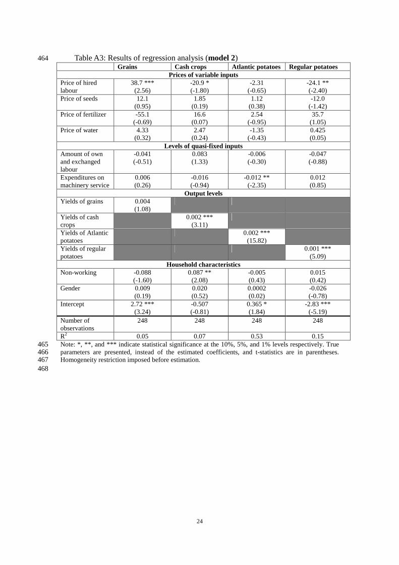
24

Table A3: Results of regression analysis (model 2) 464 Grains Cash crops Atlantic potatoes Regular potatoes


38.7 *** (2.56)

-20.9 * (-1.80)

-2.31 (-0.65)

-24.1 ** (-2.40)

Price of seeds 12.1 (0.95)

1.85 (0.19)

1.12 (0.38)

-12.0 (-1.42)

Price of fertilizer -55.1 (-0.69)

16.6 (0.07)

2.54 (-0.95)

35.7 (1.05)

Price of water 4.33 (0.32)

2.47 (0.24)

-1.35 (-0.43)

0.425 (0.05)


-0.041 (-0.51)

0.083 (1.33)

-0.006 (-0.30)

-0.047 (-0.88)


0.006 (0.26)

-0.016 (-0.94)

-0.012 ** (-2.35)

0.012 (0.85)

Output levels Yields of grains 0.004

(1.08)


0.002 *** (3.11)


0.002 *** (15.82)


0.001 *** (5.09)

Household characteristics Non-working -0.088

(-1.60) 0.087 ** (2.08)

-0.005 (0.43)

0.015 (0.42)

Gender 0.009 (0.19)

0.020 (0.52)

0.0002 (0.02)

-0.026 (-0.78)

Intercept 2.72 *** (3.24)

-0.507 (-0.81)

0.365 * (1.84)

-2.83 *** (-5.19)


248 248 248 248


468

25

Figure 1: Kernel density estimates of changes (between 2007 and 2009) in land 469 shares 470

471 472

473

0

.01

.02

.03

.04

.05

-40 -20 0 20 40 60

kernel = epanechnikov, bandwidth = 2.65

Grains

0

.02

.04

.06

.08Density

-60 -40 -20 0 20 40


Cash crops

0 1 2 3 4 5 Density

-20 -10 0 10 20

kernel = epanechnikov, bandwidth = .05

Atlantic potatoes

0

.02

.04

.06

.08

Density

-40 -20 0 20 40


Regular potatoes

Density

effects of water priority policy on farmers’ decision on...

Documents