effects of structured roughness on fluid flow at the
TRANSCRIPT

Rochester Institute of TechnologyRIT Scholar Works
Theses Thesis/Dissertation Collections
11-1-2010
Effects of structured roughness on fluid flow at themicroscale levelRebecca Noelani Wagner
Follow this and additional works at: http://scholarworks.rit.edu/theses
This Thesis is brought to you for free and open access by the Thesis/Dissertation Collections at RIT Scholar Works. It has been accepted for inclusionin Theses by an authorized administrator of RIT Scholar Works. For more information, please contact [email protected].
Recommended CitationWagner, Rebecca Noelani, "Effects of structured roughness on fluid flow at the microscale level" (2010). Thesis. Rochester Institute ofTechnology. Accessed from
Effects of Structured Roughness on Fluid Flow at the Microscale Level
by
Rebecca Noelani Wagner
A Thesis Submitted in Partial Fulfillment of the Requirements for the degree of
Master of Science in Mechanical Engineering
Approved by:
Dr. Satish Kandlikar _____________________________________
Department of Mechanical Engineering (Thesis Advisor)
Dr. Steven Weinstein _____________________________________
Department of Chemical and (Committee Member)
Biomedical Engineering
Dr. Kathleen Lamkin-Kennard _____________________________________
Department of Mechanical Engineering (Committee Member)
Dr. Alan Nye _____________________________________
Department of Mechanical Engineering (Department Representative)
Department of Mechanical Engineering
Rochester Institute of Technology
Rochester, NY 14623
November 2010

ii
Permission for Thesis Reproduction
I, Rebecca Noelani Wagner, hereby grant permission to the Wallace Memorial Library of the
Rochester Institute of Technology to reproduce my thesis entitled Effects of Structured Roughness on
Fluid Flow at the Microscale Level in whole or in part. Any reproduction will not be for commercial
use or profit.
_______________________________ ____________________
Rebecca Noelani Wagner November 19, 2010
iii
Abstract
There are no theoretical differences between microscale and macroscale flows for
incompressible liquids. Fluid flow and heat transfer characteristics in microchannels, however, are
known to deviate from conventional macroscale theory in both the laminar and turbulent regimes. As
the hydraulic diameter of a channel decreases, the effects of inherent surface roughness within the
channel becomes more apparent, causing an increase in frictional losses and early transition to
turbulence, as well as unpredictable heat transfer performance. Though many have experimentally,
analytically, and numerically established that such deviations occur, the hypotheses attempting to
characterize the deviations are sometimes contradictory and frequently employ correctional factors.
Hence, no concise and conclusive explanation has been given.
Difficulties with existing knowledge hinge around defining surface roughness itself. Average
roughness amplitude parameters are commonly in use, but do not provide sufficient representation of
designed roughness structures. Two-dimensional grooves or ridges can yield the same amplitude
values yet exhibit vastly different hydraulic and heat transfer performance.
This work aims to characterize structured surface roughness using existing parameters, and
form a theoretical model to correlate surface descriptors to fluid performance in rectangular channels
of varying aspect ratios and surface geometries. A theoretical model was developed to predict the
effect of roughness pitch and height on pressure drop along the channel length, using friction factors
for comparison with prior work. Validation of the proposed theory was carried out through
experimentation with water flow in channels possessing designed transverse rib roughness. The end
goal was to develop a clear understanding of the effect of two-dimensional structured roughness on
frictional losses in fully-developed laminar flow, with the potential for extension to analysis of heat
transfer and developing flow.

iv
Table of Contents
Abstract .................................................................................................................................... iii
Table of Contents ..................................................................................................................... iv
List of Figures .......................................................................................................................... vi
List of Tables ......................................................................................................................... viii
Nomenclature ........................................................................................................................... ix
1 Introduction ......................................................................................................................1
2 Related Work ....................................................................................................................3
2.1 Historical Perspective ..............................................................................................3
2.2 Channel Geometry ...................................................................................................4
2.3 Uniform Roughness .................................................................................................6
2.4 Structured Roughness ..............................................................................................8
2.5 Roughness Models ...................................................................................................9
2.6 Objectives ..............................................................................................................10
3 Theoretical Model ..........................................................................................................12
3.1 Fundamental Equations and Computational Domain ............................................12
3.2 Assumptions and System of Equations .................................................................13
3.2.1 Lubrication Approximation ...................................................................................... 14
3.2.2 Simplified System of Equations ............................................................................... 15
3.3 Wall Function Method ...........................................................................................16
3.3.1 Structured Roughness ............................................................................................... 16
3.4 Constricted Flow Method ......................................................................................17
3.4.1 Surface Roughness and Channel Separation ............................................................ 18
3.5 Further Theoretical Analysis .................................................................................20
3.6 Application of Theory ...........................................................................................22
4 Preliminary Results ........................................................................................................23
4.1 Saw-tooth Roughness ............................................................................................23
4.2 Idealized Roughness ..............................................................................................27
4.3 Friction Factors ......................................................................................................31
4.4 Flow through Channels Possessing Idealized Roughness .....................................36
5 Experimental Setup ........................................................................................................39
5.1 Design Parameters .................................................................................................39
5.2 Structured Roughness ............................................................................................40
v
5.3 Channel Assembly .................................................................................................45
5.4 Test Loop ...............................................................................................................48
5.5 Calibration and Experimental Uncertainty ............................................................49
5.5.1 Pressure Transducer Calibration ............................................................................... 50
5.5.2 Flowmeter Calibration .............................................................................................. 50
5.5.3 Thermocouple Calibration ........................................................................................ 51
5.5.4 Bias and Precision Error ........................................................................................... 51
6 Results and Discussion ...................................................................................................57
6.1 Validation of Test Set with Hydraulically Smooth Channels ................................57
6.2 Structured Roughness Results ...............................................................................60
6.3 Comparison with Wall Function Method ..............................................................69
6.4 Comparison with Constricted Flow Model ...........................................................78
7 Conclusions ....................................................................................................................79
8 Recommendations ..........................................................................................................81
9 References ......................................................................................................................83
Appendix A – MATLAB Code............................................................................................. A-1
Appendix B – Test Matrices ..................................................................................................B-1
Appendix C – Part Drawings .................................................................................................C-1
vi
List of Figures
Figure 1. Channel Geometry and Axis Orientation .................................................................12
Figure 2. Computational Domain ............................................................................................13
Figure 3. Trajectory of a Fluid Particle and its Velocity Components ....................................14
Figure 4. Profilometer Data for 815 μm Pitch Saw-tooth Roughness Profile .........................18
Figure 5. Representative Channel and Roughness Geometry; h = 100 μm, λ = 400 μm,
b = 400 μm ..............................................................................................................19
Figure 6. Smooth Channel Validation of Previous Experimental Setup .................................23
Figure 7. Saw-tooth Roughness Profile with Height Parameters, λ = 503 μm ........................24
Figure 8. Curve Fit of 503 μm Pitch Saw-tooth Roughness Profile ........................................25
Figure 9. f vs. Re for 503 μm Pitch Surface, b = 400 μm ........................................................26
Figure 10. f vs. Re for 503 μm Pitch Surface, b = 300 μm ......................................................26
Figure 11. Roughness Parameters vs. λ/h for λ = 250 μm and p = 6 .......................................28
Figure 12. Ideal Surface Roughness Profiles for h = 50 μm, λ varies, p varies .......................29
Figure 13. Roughness Parameters vs. λ/h for λ = 250 μm, p varies .........................................29
Figure 14. Roughness Parameters vs. λ/h for h = 50 μm, p varies ...........................................30
Figure 15. Friction Factor vs. Aspect Ratio, Smooth Channel Correlation .............................32
Figure 16. Friction Factor vs. Aspect Ratio, Constricted Flow Method, Re = 50 ...................33
Figure 17. Friction Factor vs. Aspect Ratio, Wall Function Method, Re = 50 ........................34
Figure 18. Comparison of Wall Function Method with Smooth Channel Correlation,
for Channel Separation b = 150 μm ........................................................................37
Figure 19. Comparison of Wall Function Method with Smooth Channel Correlation,
for Surface Profile λ/h = 5 .......................................................................................38
Figure 20. Designed Roughness Profile, h = 50 μm, λ = 150 μm ............................................40
Figure 21. Laser Confocal Image of Wire EDM Result, Rstep = 49.6 μm, RSM = 149.8 μm ....41
Figure 22. Curve-fit and Profile Data of Surface Designed for h = 50 μm, λ = 150 μm .........42
Figure 23. Measured Amplitude Parameters vs. Designed Height ..........................................43
Figure 24. Shape Parameters vs. Power ...................................................................................44
Figure 25. Solid Model of Roughness Test Piece ....................................................................45
Figure 26. Solid Model of Gauge Block ..................................................................................46
vii
Figure 27. Solid Model of Microchannel Assembly ................................................................47
Figure 28. Solid Model of Test Set Assembly (rear view) ......................................................47
Figure 29. Schematic of Experimental Test Loop ...................................................................49
Figure 30. Smooth Channel Friction Factor vs. Reynolds Number, ........................................59
Figure 31. Smooth Channel Experimental vs. Theoretical Friction Factors ............................60
Figure 32. Deviation in Channel Separation Measured Before and After Flow Testing .........61
Figure 33. Experimental Friction Factor vs. Reynolds Number, λ/h = 7 .................................64
Figure 34. Experimental Friction Factor vs. Reynolds Number, λ/h = 8 .................................65
Figure 35. Experimental Friction Factor vs. Reynolds Number, λ/h = 5 .................................66
Figure 36. Experimental Friction Factor vs. Reynolds Number, λ/h = 3 .................................67
Figure 37. Experimental Friction Factor vs. Reynolds Number, λ/h = 2 .................................68
Figure 38. Experimental and Theoretical Friction Factor vs. Reynolds Number, λ/h = 7 .......70
Figure 39. Experimental and Theoretical Friction Factor vs. Reynolds Number, λ/h = 8 .......71
Figure 40. Experimental and Theoretical Friction Factor vs. Reynolds Number, λ/h = 5 .......72
Figure 41. Experimental and Theoretical Friction Factor vs. Reynolds Number, λ/h = 3 .......73
Figure 42. Experimental and Theoretical Friction Factor vs. Reynolds Number, λ/h = 2 .......74
Figure 43. Experimental Poiseuille Number vs. Channel Aspect Ratio ..................................76
Figure 44. Constricted Experimental Friction Factor vs. Reynolds Number, λ/h = 3 .............78
viii
List of Tables
Table 1. Test Matrix Summary: Roughness Geometry - Designed .........................................39
Table 2. Test Matrix Summary: Channel Geometry - Designed .............................................39
Table 3. Roughness Parameters ...............................................................................................42
Table 4. Instrument Bias and Precision Error ..........................................................................55
Table 5. Laminar and Turbulent Precision Error .....................................................................55
Table 6. Parameter Error ..........................................................................................................56
Table 7. Measured Channel Geometry – Smooth Surfaces .....................................................58
Table 8. Test Matrix Summary: Roughness Geometry - Measured ........................................61
Table 9. Test Matrix Summary: Channel Geometry - Measured.............................................62
Table 10. Experimental Error ..................................................................................................75
Table 11. Experimental Poiseuille Numbers ...........................................................................77
Table 12. Designed Test Matrix.............................................................................................B-1
Table 13. Measured Test Matrix ............................................................................................B-2

ix
Nomenclature
Latin
A Area, surface or cross-sectional,
as noted in the text
a Rectangular channel height, or
longer of the two dimensions
b Rectangular channel separation, or
smaller channel dimension
beff Effective channel separation
D Pipe diameter
Dh Hydraulic diameter
e Roughness size, used in the
Moody diagram [1]
Fp Average floor profile
(alternatively named FdRa)
f Friction factor
f(x) Lower wall function
g Gravity
g(x) Upper wall function
h Roughness height, wall function
method
k Roughness height, as defined by
Von Mises [2]
P Pressure
Q Volumetric flow rate
r Pipe radius
Ra Average roughness
Rc Average height
RΔq RMS tilt
Re Reynolds number
Rku Kurtosis
Rp Maximum peak height
Rq Root-mean-square (RMS)
roughness
Rsk Skew
RSM Mean spacing of peaks
Rv Minimum valley height
Rz Maximum or ten-point-peak
height
u x-component of velocity
v y-component of velocity
w z-component of velocity
Greek
α Channel aspect ratio; smaller
dimension divided by larger
δ boundary layer thickness
Δa Mean slope of roughness profile
εFp Roughness height parameter, for
constricted flow model [3]
λ Roughness pitch
μ Dynamic viscosity
ρ Density
Subscripts
cf Constricted flow
1
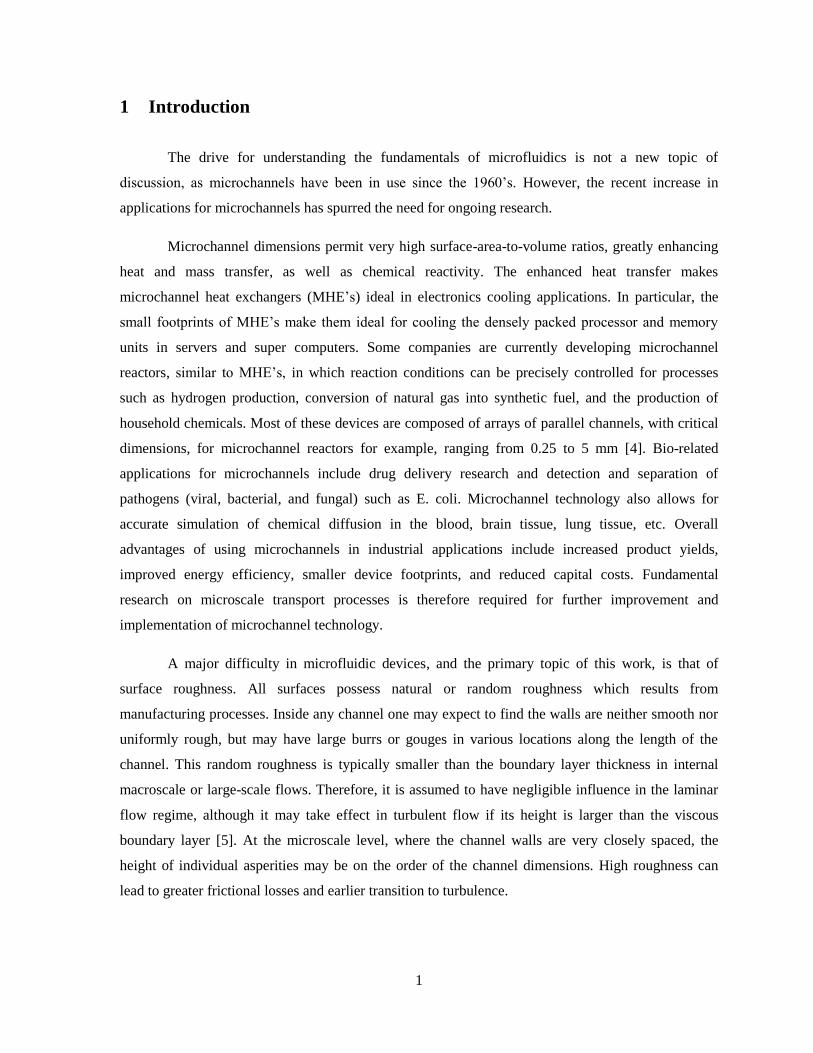
1 Introduction
The drive for understanding the fundamentals of microfluidics is not a new topic of
discussion, as microchannels have been in use since the 1960‟s. However, the recent increase in
applications for microchannels has spurred the need for ongoing research.
Microchannel dimensions permit very high surface-area-to-volume ratios, greatly enhancing
heat and mass transfer, as well as chemical reactivity. The enhanced heat transfer makes
microchannel heat exchangers (MHE‟s) ideal in electronics cooling applications. In particular, the
small footprints of MHE‟s make them ideal for cooling the densely packed processor and memory
units in servers and super computers. Some companies are currently developing microchannel
reactors, similar to MHE‟s, in which reaction conditions can be precisely controlled for processes
such as hydrogen production, conversion of natural gas into synthetic fuel, and the production of
household chemicals. Most of these devices are composed of arrays of parallel channels, with critical
dimensions, for microchannel reactors for example, ranging from 0.25 to 5 mm [4]. Bio-related
applications for microchannels include drug delivery research and detection and separation of
pathogens (viral, bacterial, and fungal) such as E. coli. Microchannel technology also allows for
accurate simulation of chemical diffusion in the blood, brain tissue, lung tissue, etc. Overall
advantages of using microchannels in industrial applications include increased product yields,
improved energy efficiency, smaller device footprints, and reduced capital costs. Fundamental
research on microscale transport processes is therefore required for further improvement and
implementation of microchannel technology.
A major difficulty in microfluidic devices, and the primary topic of this work, is that of
surface roughness. All surfaces possess natural or random roughness which results from
manufacturing processes. Inside any channel one may expect to find the walls are neither smooth nor
uniformly rough, but may have large burrs or gouges in various locations along the length of the
channel. This random roughness is typically smaller than the boundary layer thickness in internal
macroscale or large-scale flows. Therefore, it is assumed to have negligible influence in the laminar
flow regime, although it may take effect in turbulent flow if its height is larger than the viscous
boundary layer [5]. At the microscale level, where the channel walls are very closely spaced, the
height of individual asperities may be on the order of the channel dimensions. High roughness can
lead to greater frictional losses and earlier transition to turbulence.

2
Surface roughness is typically characterized by the use of average amplitude parameters.
These conventional amplitude parameters are in common use because they are simple to calculate and
provide a sufficient description of natural roughness in macroscale applications. In order to
understand the effect of asperity height, slope, density, etc. of roughness on fluid flow, it is useful to
consider structured roughness so as to both control and measure those aspects of surface geometry
individually. The average amplitude parameters which are sufficient for uniform roughness are
insufficient in representing structured or periodic roughness.

3
2 Related Work
2.1 Historical Perspective
Since Darcy identified the dependence of internal fluid flow on pipe diameter, inclination,
and surface type in the 1800‟s [6], much effort has gone into experimental and theoretical
assessments of the effects of roughness on internal flows. In the early 1900‟s, Von Mises highlighted
the significance of relative roughness, which he defined as the ratio of roughness “size” to pipe
radius, k/r [2]. Hopf [7] and Fromm [8] later performed flow experiments on rectangular channels
with various types of roughness. They classified surface types based on roughness aspect ratios and
concluded that friction factor and Reynolds number are dependent on the surface type, differentiated
by the roughness pitch-to-height ratio, λ/h, for repeating roughness structures. In an attempt to expand
the understanding of flow in rough pipes at the time, Nikuradse performed exhaustive experiments
assessing a complete range of Reynolds numbers for various k/r values, while maintaining geometric
similitude in pipe geometries, resulting in an enormous database for frictional flow in pipes [9]. In
1939, Colebrook developed the general (and well-known) formula for friction factor at high Reynolds
numbers [10]. With Nikuradse‟s experimental results and Colebrook‟s turbulent flow formula, Moody
[1] constructed a convenient means, in graphical form, for estimating friction factors based on relative
roughness and Reynolds number, making the Darcy-Weisbach equation more readily applicable.
The Moody diagram allows for prediction of fluid behavior in macroscale pipes, and has been
in use in both academic and industry settings for decades. The diagram is limited to relative
roughness values of 5% and lower, or e/D < 0.05, however, and indicates that roughness of any size
has no effect on friction factors in the laminar flow regime. This conclusion that roughness takes no
effect in laminar flows is still pervasive today in that the flow in conventional-sized pipes and
channels is typically turbulent, so the variance in the friction factors for laminar flows are of less
practical importance. Interest in microscale phenomena has increased in the recent past due to its
usefulness for passive enhancement of microfluidic devices. With the increase in the use of
microscale geometries in various applications, and because flows in microscale pipes and ducts are
often laminar, the study of laminar flow in roughened microchannels is of significant importance.
Experiments performed since the 1980‟s indicate that as the pipe size decreases there is significant
deviation from conventional theory in both laminar and turbulent regimes [11].

4
2.2 Channel Geometry
Early research on internal flows focused on circular ducts or conventional pipes, as was the
case with the data used to generate the Moody diagram. For fully developed, laminar flow in circular
ducts, the Darcy friction factor may be defined as 64/ReD, where ReD is the Reynolds number
calculated using the pipe diameter as the characteristic length. This definition of laminar friction
factor does not hold true for non-circular geometries, since the wall shear varies around the perimeter
of the duct. In order to extend conventional correlations for non-circular geometries, the hydraulic
diameter may be used in place of the characteristic length;
P
AD h
4
where A is the cross-sectional area and P is the wetted perimeter, or the length of the wall in contact
with the fluid flowing through the cross-section. For a rectangular cross-section in which one side is
significantly smaller than the other, Dh limits to twice the smaller dimension. This concept of
hydraulic diameter is used simply to extend existing empirical correlations for pipe flow to non-
circular geometries, and to represent the characteristic length scale in fluid mechanics.
Throughout the 1970‟s, Shah worked to analyze the variation of fully developed, laminar
flow friction factors in smooth ducts of various cross sectional geometries using a least-squares-
matching technique [12, 13]. His work resulted in a compilation of analytical solutions for flow
friction based on data from over 300 sources for 25 duct geometries. These solutions are still used for
comparison to this day, and are likewise used for smooth channel comparison in this work.
In more recent literature, researchers have reported that friction factors in non-circular
geometries begin to differ from Shah‟s findings as the channel size decreases to the microscale level.
In gas flows, the discrepancy may be attributed to slip flow at the boundaries, but this does not
explain the difference for incompressible flows. Prior works on liquid flow in microchannels have
reported significant increases [14-17] or decreases [18, 19] in friction factors from conventional
laminar theory, while others reported negligible deviations [20-24]. In addition to these, other authors
have reported increases in friction factors for some geometries or aspect ratios, but decreases for
others [25, 26]. Many of these authors highlighted the role of wall roughness in their observed
deviations.
5
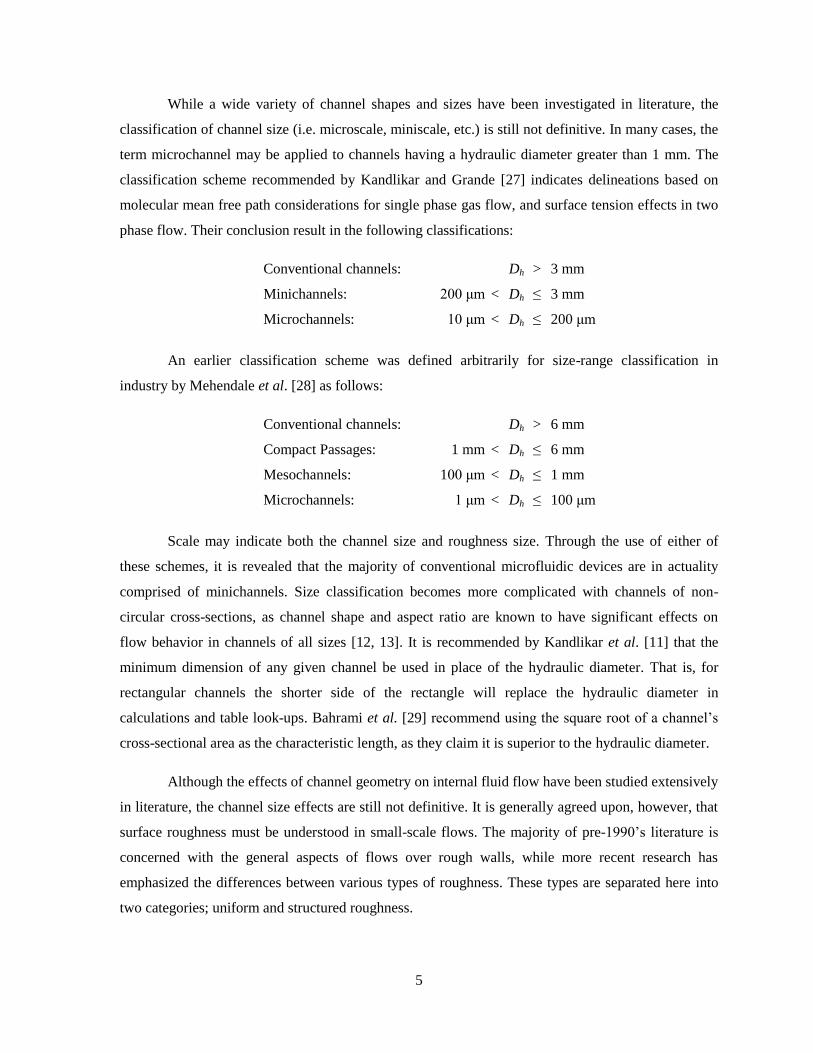
While a wide variety of channel shapes and sizes have been investigated in literature, the
classification of channel size (i.e. microscale, miniscale, etc.) is still not definitive. In many cases, the
term microchannel may be applied to channels having a hydraulic diameter greater than 1 mm. The
classification scheme recommended by Kandlikar and Grande [27] indicates delineations based on
molecular mean free path considerations for single phase gas flow, and surface tension effects in two
phase flow. Their conclusion result in the following classifications:
Conventional channels: Dh > 3 mm
Minichannels: 200 μm < Dh ≤ 3 mm
Microchannels: 10 μm < Dh ≤ 200 μm
An earlier classification scheme was defined arbitrarily for size-range classification in
industry by Mehendale et al. [28] as follows:
Conventional channels: Dh > 6 mm
Compact Passages: 1 mm < Dh ≤ 6 mm
Mesochannels: 100 μm < Dh ≤ 1 mm
Microchannels: 1 μm < Dh ≤ 100 μm
Scale may indicate both the channel size and roughness size. Through the use of either of
these schemes, it is revealed that the majority of conventional microfluidic devices are in actuality
comprised of minichannels. Size classification becomes more complicated with channels of non-
circular cross-sections, as channel shape and aspect ratio are known to have significant effects on
flow behavior in channels of all sizes [12, 13]. It is recommended by Kandlikar et al. [11] that the
minimum dimension of any given channel be used in place of the hydraulic diameter. That is, for
rectangular channels the shorter side of the rectangle will replace the hydraulic diameter in
calculations and table look-ups. Bahrami et al. [29] recommend using the square root of a channel‟s
cross-sectional area as the characteristic length, as they claim it is superior to the hydraulic diameter.
Although the effects of channel geometry on internal fluid flow have been studied extensively
in literature, the channel size effects are still not definitive. It is generally agreed upon, however, that
surface roughness must be understood in small-scale flows. The majority of pre-1990‟s literature is
concerned with the general aspects of flows over rough walls, while more recent research has
emphasized the differences between various types of roughness. These types are separated here into
two categories; uniform and structured roughness.

6
2.3 Uniform Roughness
The surface roughness used in many experiments can be classified as uniform or Gaussian
roughness. That is, the amplitude density distribution for the data obtained from a profilometer,
microscope, or other metrology device is a normal or Gaussian distribution. When glass is etched or
metals are abraded, the outcome is frequently Gaussian. The roughness that results naturally from
various machining and manufacture techniques is random, but frequently Gaussian. The difference is
that random roughness is not controlled or deliberate, whereas etching or polishing is done in order to
obtain a desired surface finish. A skewed distribution is indicative of prominent peaks or valleys
across a surface, but in general the same geometry would be found uniformly across an etched or grit
blasted surface.
The Moody diagram is based heavily on experimental data for uniformly rough surfaces.
Nikuradse, for example, sifted and re-sifted sand so that the grain diameters were approximately the
same, then used a lacquer to adhere the sand to the inner surfaces of pipes [9]. Since then, authors
have attempted to equate surface roughness to an equivalent sand grain roughness. Such an approach
to roughness characterization is questionable as the method of gluing sand to a surface may not result
in roughness that is the same size as the sand grains, nor could repeating Nikuradse‟s method result in
the same density or distribution of grains on the surface. Any slight difference in coating or drying the
sand could result in different flow resistance. While the size of uniform roughness may be controlled
in this technique, the distribution is entirely uniform across the surface and is difficult to characterize
by anything other than amplitude parameters, hence the desire to use an equivalent sand grain
roughness for comparison.
Existing roughness parameters primarily serve to describe natural or uniform roughness by
the average or extreme height. Standard amplitude parameters include the average roughness, Ra,
which is the arithmetic mean of surface height values, and the root-mean-square (RMS) roughness,
Rq, which is the standard deviation of the height distribution. Line measurements are represented by
R, whereas surface measurements are represented by S. Most amplitude parameters use the average
roughness as a reference line. Extreme height parameters, for example, represent the highest peaks or
deepest gouges in a surface relative to the mean line. In Nikuradse‟s experiments, the use of the sand
grain diameter for the roughness value is comparable to using an extreme amplitude parameter to
represent the surface in that the sand particles would not actually project into the boundary layer to
their full diameter due to the laquer coating. Amplitude parameters are useful for surface specification
and control in design and manufacturing, but cannot effectively predict hydraulic performance.

7
Alternative roughness parameters may contribute to the prediction of hydraulic performance,
but are not in common use for fluid flow applications. The skew of a surface, Rsk, represents the
symmetry of that profile about its meanline, indicating whether it possesses many sharp peaks
(positive skewness), sharp valleys (negative skewness), or is a Gaussian distribution (Rsk = 0).
Kurtosis, Rku, represents the peakedness of a surface, qualifying the flatness of the amplitude density
distribution. A leptokurtic surface (Rku > 3) possesses frequent extreme peaks and valleys, as opposed
to a platykurtic surface which exhibits infrequent or small deviations. There are also parameters for
counting the number of times a profile crosses a threshold, and for evaluating the density or slopes of
peaks. These and many other spatial or functional parameters have potential for use in predicting
surface effects on fluid flows.
Menezes et al. [30] roughened steel surfaces with wet and dry emery paper in various
patterns in order to correlate twenty five existing roughness parameters, including skew and kurtosis,
with the coefficient of friction for each surface under lubricated conditions. He found that the
performance of each plate was independent of the average roughness Ra, but correlated well with the
mean slope of the profile Δa for every surface. This parameter is the arithmetic mean of the slopes
between every pair of successive points of a roughness profile, giving an indication of the shape of
the profile. Although it compared well in the reported experiments, it does not completely describe a
surface and may need to be combined with an amplitude or hybrid parameter. No conclusion was
made for the skew or kurtosis parameters, though it was implied that these were unable to be
correlated with the frictional coefficient.
In 2005, Kandlikar et al. [3] proposed the use of a constricted parameter for use in estimating
pressure drop in roughened microchannels. The parameter εFp is a function of the average roughness
and two other amplitude parameters, and serves to account more accurately for the extent to which
roughness elements project into the boundary layer. This constricted flow approach led to a modified
Moody diagram which covers higher relative roughness values and smaller hydraulic diameters. This
approach is valid provided that the roughness elements are closely spaced. There is still a need,
however, for further understanding the effect of roughness geometry on internal flows.

8
2.4 Structured Roughness
Structured or artificial roughness was studied at least as far back as the 1920‟s with Hopf and
Fromm‟s saw-tooth style two-dimensional roughness [7, 8], followed by Schlichting‟s three-
dimensional arrays of spheres, cones, and angled roughness [31]. Structured roughness is obtained by
adding or removing material from a surface in a deliberate and precise way such that a two- or three-
dimensional pattern arises. Though the focus for these authors was on turbulent flow, they were some
of the pioneers in artificial roughness studies.
As there is no “universal” parameter for structured roughness, many researchers have resorted
to using roughness height values and relative roughness in order to assess and compare the effects of
different roughness geometries on fluid flow, even in recent literature. Schlichting, who used an
equivalent sand grain roughness in his study, also attempted to correlate the flow resistance with
roughness density, quantified by the projected roughness area normal to flow divided by the total
plate area. In 1952, Sams [32] experimented with structured roughness in laminar and turbulent flow
by threading and cross-threading macroscale pipes (D ≈ 12.7 mm). He concluded that the
conventional “relative roughness” concept is not sufficiently representative of the effects of structured
roughness, specifically his square thread type roughness, on hydraulic performance. Though the
author went to great lengths to correlate friction factors with the square roughness height, width, and
spacing, the final outcomes were a series of empirical formulations.
Numerical simulations have been employed for assessing structured roughness effects in
microchannel flow by a number of researchers, either through the use of commercial CFD software or
by programming finite difference methods manually in languages such as FORTRAN or computing
environments like MATLAB, etc. Rawool et al. [33] simulated laminar air flow in microchannels
possessing two-dimensional transverse rib roughness, and systematically varied the roughness cross-
section from triangular to trapezoidal to rectangular, as well as varying the height and pitch, or peak-
to-peak distance. The authors found that the roughness pitch plays a definite role in fluid flow, in that
the friction factor increases as roughness elements are brought closer together, i.e. higher friction
factors for smaller pitch values. This was in addition to the roughness height effect already seen in
previous literature; friction factor increases as roughness height increases. Friction factors were also
found to be greater for triangular and rectangular geometries, and lower for trapezoidal roughness.
These results are in agreement with the numerical simulations of Wang et al. [34] and Sun and Faghri
[35], enforcing the idea that the roughness geometry should be taken into consideration.
9
Transition to turbulence is frequently correlated to the ratio of roughness height to boundary
layer thickness k/δ, which highlights the importance of the interaction of roughness elements with the
boundary layer. In a review on turbulent flows over transverse rib type roughness, Jiménez [36]
described two types of roughness; d-type and k-type, and a transitional roughness that occurs between
these two types. They d-type roughness was described as ribs closely spaced such that they can
sustain stable vortices (recirculation downstream of the roughness elements) that serve to isolate the
bulk flow from the roughness. The k-type roughness is sparser such that the flow separates at the top
of the roughness element and reattaches downstream, before reaching the next roughness element.
The vortices interact with the bulk flow for this sparse roughness, causing increased friction factors
and early transition to turbulence. Coleman et al. [37] experimentally and numerically assessed the
effect of transverse rib roughness pitch-to-height ratios, λ/h, on turbulent flow and identified
“transitional” roughness, at λ/h ≈ 8, as having the most predominant effect on fluid flow. The authors
reported that values of λ/h < 5 indicate closely spaced ribs, d-type roughness, or skimming flow,
while λ/h > 5 indicate isolated roughness elements, k-type roughness, or interactive flow. In the
extremes where λ/h is significantly greater or less than 5, the roughness effect is expected to diminish.
Although these publications discussing roughness ratios focus on turbulent flows, the concept may
still hold true for microscale laminar flows.
2.5 Roughness Models
As stated previously, there are no theoretical differences between microscale and macroscale
flows for incompressible liquids. Some authors, however, have made modifications to conventional
theory in order to account for microscale roughness effects. In this section, a few of those models for
flow in rough microchannels are reviewed. These models were either developed for or have been
applied to steady, laminar, fully-developed liquid flows in microchannels possessing uniform or
structured roughness.
Mala and Li [38] proposed the roughness-viscosity model (RVM), in which the surface
roughness increases the fluid viscosity near the wall, accounting for the increase in friction factor in
laminar flow. The authors define roughness-viscosity as a function of distance from the wall, such
that the roughness-viscosity is zero at the center of the channel and a positive, non-zero, finite value
at the wall. The concept is that the surface roughness increases momentum transfer in the boundary
layer near the wall. But this model includes a coefficient that must be determined experimentally.
10
Sabry [39] took a unique approach that is reminiscent of the Cassie-Baxter model for surface
wetting; the liquid does not fully contact the rough walls, and gases are trapped between some
roughness elements. Conceptually, in this model, when flow separation occurs over roughness
elements, the flow will become separated from the wall by a thin film of gas. The author initially
assumed a “blanket” of gas of a specified thickness completely separates the bulk liquid from the
rough wall. Since, in actuality, a gas blanket could not completely separate the liquid from the solid, a
shielding coefficient was introduced into the model. This correction factor would range from 0 for no
entrained gas to 1 for total separation of liquid from solid. Though the concept may be of interest in
heat transfer applications, as a vapor blanket would be likely to occur and would insulate the flow,
this model does not address the variation in friction factor with roughness height, as has been
observed in previous literature.
Koo and Kleinstreuer [40], and Kleinstreuer and Koo [41], proposed a porous medium layer
(PML) model in which uniform or random surface roughness is represented by a porous region or
layer on the walls of a channel. The surface roughness (or PML) can increase or decrease the friction
factor, depending on the PML permeability. The authors found good agreement with previous data.
However, the model requires a number of unique and obscure parameters, such as porosity,
permeability, and resistance speed factor, resistance speed power, and resistance constant. Constraints
for the resistance variables were stated, but their exact definitions were not clear.
Expanding on the PML model, Gamrat et al [42, 43] developed a roughness layer model
(RLM) in which they employed a discrete element approach to represent roughness at the wall. The
authors used two effective roughness height parameters that are dependent on two dimensionless
parameters; porosity of the “rough layer” and roughness height normalized by roughness spacing. The
authors reported good agreement with experimental data for both uniform and structured roughness.
But, the model is semi-empirical, as a drag coefficient must be obtained experimentally.
2.6 Objectives
Definite departure from conventional laminar theory has been identified in numerous
experiment-based publications. Vast portions of the experimental works have resulted in empirical
relations, scaling factors, etc., and these correlations are not universally applicable across the full
range of small-scale channels, roughness types, and fluids. Similarly, recent theoretical and numerical
11
works result in scaling models or require correction factors. Although it is intuitive that flow over a
rough surface will experience greater drag than a smooth surface, it is still unclear when, where, and
how a rough surface will begin to affect the bulk flow.
The study described herein deals with laminar water flow in rectangular channels of small
aspect ratios, primarily in what may be considered the minichannel range, but touches on the
microscale regime. Structured roughness is evaluated for its controllability of pitch and height. This
work is an extension of a series of experiments performed by Brackbill [44] with saw-tooth roughness
in rectangular microchannels. Standard amplitude parameters were evaluated as well as spatial and
functional parameters in order to determine a combination of parameters relevant to structured
roughness surface description. The relative roughness, εFp/Dh, and the ratio of roughness height to
channel separation, h/b, were also assessed for comparison with prior works. It is shown here that
flow between rough walls can be modeled without the detailed computation of the flow around the
roughness elements themselves.

12
3 Theoretical Model
Two-dimensional structured roughness was studied for its controllability of height, pitch, and
slope of periodic peaks. A theoretical flow model that incorporates descriptive roughness parameters
was developed, with focus on fully developed laminar flow.
3.1 Fundamental Equations and Computational Domain
The Navier-Stokes (N-S) equations for an incompressible Newtonian fluid form the
foundation for the theoretical treatment of the microscale problem presented here. The result of the
analysis provides pressure as a function of velocity, fluid properties, and channel and roughness
geometry. In addition, the continuity equation was used to complete the relationship between
volumetric flow rate and pressure terms. The internal two-dimensional flow was assumed to be steady
and fully developed, so that inlet and outlet effects may be neglected. For further simplification, fluid
properties were assumed to be constant.
Channel orientation and geometry are displayed in Figure 1 below. Fluid flow is in the
positive x-direction, transverse rib roughness is in the x-y plane, and gravity acts in the negative y-
direction. The channel separation b is significantly less than the channel length L, and the channel
aspect ratio is small, such that the flow is comparable to flow between infinite parallel plates.
Figure 1. Channel Geometry and Axis Orientation

13
The computational domain is the region between the rough walls, in the x-z plane. The
boundaries for the flow is the transverse rib roughness, represented by the functions f(x) and g(x) for
the lower and upper walls, respectively, as seen in Figure 2. This periodic roughness is described by
its pitch λ and height h. Channel separation b is the difference between wall functions f(x) and g(x).
The treatment of the separation b is discussed in the Surface Roughness and Channel Separation
section. The limits of integration in the x-direction are from 0 to L.
Figure 2. Computational Domain
3.2 Assumptions and System of Equations
This is a two-dimensional analysis, for which the velocity vector is kwiuu ˆˆ
. Flow is
assumed to be steady, meaning any time derivatives are zero, resulting in a parabolic flow profile,
which is validated in this section. The fluid is an incompressible liquid, for which the density and
viscosity are constant. Gravity acts in the y-direction only, perpendicular to the computational domain
shown in Figure 2 above. Inlet and outlet effects are neglected. The no-slip boundary condition is
applied, i.e. velocity at the walls, where )(xfz and )(xgz , is zero. In addition, it is assumed
that the pressure at the inlet and outlet, or P0 and PL, respectively, are known.
The momentum equation, Newton‟s second law of motion, balances the acceleration of a
fluid element and the forces imposed on it by neighboring elements. The continuity equation

14
expresses conservation of mass for a constant density fluid. These comprise the system of equations
used for the current analysis:
0:
z
w
x
uContinuity
z
ww
x
wu
z
w
x
w
z
Pcomponentz
y
Pgcomponenty
z
uw
x
uu
z
u
x
u
x
Pcomponentx
SN
2
2
2
2
2
2
2
2
:
0:
:
3.2.1 Lubrication Approximation
To solve the full N-S equations requires the use of computational fluid dynamics. In this
analysis, the lubrication approximation was applied for simplification by assuming that the slope of
the trajectory of fluid elements is small. That is, velocity w in the z-direction is significantly less than
velocity u in the x-direction. Figure 3 provides a visual representation of this assumption.
Figure 3. Trajectory of a Fluid Particle and its Velocity Components
Also referred to as the small slope approximation, it may be interpreted as; the slope of the
boundaries is small at every point, such that 1)(
x
xf and 1
)(
x
xg. This approximation is
often applied to flow fields in which the fluid is forced to move between two closely spaced surfaces,
as with flow between infinite parallel plates or in a slot [45], where b/L << 1.

15
3.2.2 Simplified System of Equations
Application of the lubrication approximation makes no change to the continuity equation, but
reduces the conservation of momentum equations thus:
0:
:
:2
2
z
Pcomponentz
gy
Pcomponenty
z
u
x
Pcomponentx
SN
In the x-direction, all that remains is the viscous effects. Gravity only takes effect in the y-
direction and may be used to assess variation of velocity in the y-direction. All inertial terms drop out
due to the lubrication approximation. The lack of inertia implies very low Reynolds numbers (Stoke‟s
flow) or flow in a slot of low relative roughness (small slope).
Integrating the x- and y-components of the simplified N-S equations and applying the no-slip
boundary conditions yields the following:
)(xpgyP (1)
)()(2
1xfzxgz
x
Pu
(2)
Equation 1 allows for an understanding of the effect of gravity on flow. It may be used to
evaluate changes in the flow field in the y-direction. Equation 2 represents the bulk flow velocity
profile in the absence of inertia. In laminar flow, if the channel separation b is significantly less than
the length L, then the flow is approximately parabolic, as is this bulk profile. In an extended analysis,
in section 3.5, this velocity profile serves as a trial function in an augmented lubrication
approximation in which the inertial terms in the x-component are not discounted.
Integration of the continuity equation across the channel separation brings about a volumetric
flow rate per unit depth relation. Applying Leibniz Rule, and utilizing equation 2 as an initial
approximation for the velocity profile results in the following pressure–flow relation:
a
Qxfxg
x
P
3)()(
12
1
(3)
16
Rearranging for the differential pressure term as a function of flow:
3)()(
112
xfxga
Q
x
P
(4)
Integrating this differential equation along a specified length results in an equation for
pressure-drop as a function of flow rate, viscosity, and the boundaries or wall function equations:
L
L xxfxga
QPP
0
30)()(
112 (5)
From here, equations for g(x) and f(x) are used to evaluate the integral and thereby predict the
pressure drop along the length of rough channel. These two equations are the wall functions that
represent structured two-dimensional roughness, and so this approach is referred to as the wall
function method.
3.3 Wall Function Method
Pressure drop along a length of rectangular channel may now be predicted, provided that the
channel and roughness geometries, fluid properties, and flow rate are known. Because the intention of
this study was to investigate the effects of structured roughness on laminar fluid flow, it was
necessary to utilize these wall functions f(x) and g(x) in such a way that the height and pitch of evenly
spaced peaks may be systematically varied.
3.3.1 Structured Roughness
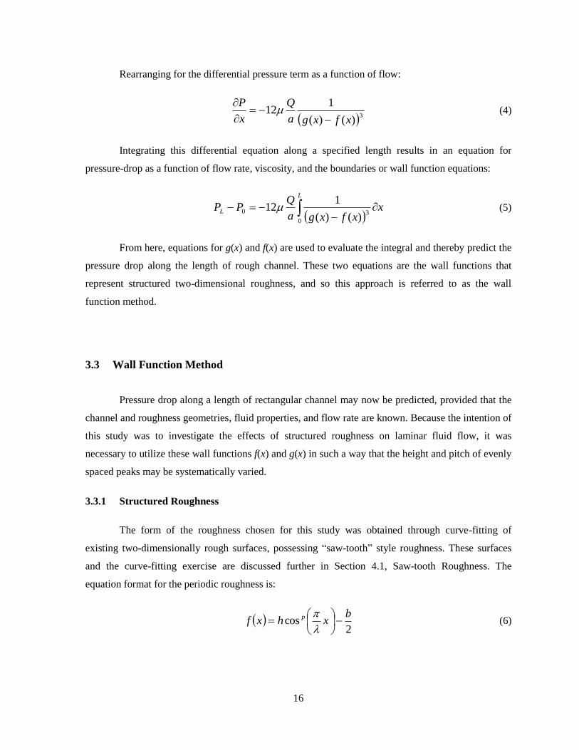
The form of the roughness chosen for this study was obtained through curve-fitting of
existing two-dimensionally rough surfaces, possessing “saw-tooth” style roughness. These surfaces
and the curve-fitting exercise are discussed further in Section 4.1, Saw-tooth Roughness. The
equation format for the periodic roughness is:
2
cosb
xhxf p
(6)
17
where h is the height of roughness elements, λ is the pitch or peak-to-peak spacing, p is the power on
the cosine which controls the slope of the peaks, and b is the root channel separation, measured
valley-to-valley. The opposing wall g(x) is the negative of equation 6 (refer to Figure 2). Thus, the
difference between these two functions results in the root channel separation minus a power sinusoid
that is a function of x.
xhbxfxg p
cos2)( (7)
This form of two-dimensional roughness is convenient in that it allows for control of all
parameters of interest, such that any one variable may be manipulated while keeping the remaining
geometries constant. To evaluate the effect of alignment of roughness peaks on fluid flow, a phase
shift variable may be added into the cosine function of one of the walls.
Implementing this style of roughness is not trivial for the theoretical model at hand. The
integral in equation 5 is difficult to solve exactly, and requires the use of averaging techniques when
boundaries of the form of equation 6 are used for the wall function input. Therefore, the Gaussian
quadrature rule was used to approximate the integral. Code was written in MATLAB in order to
expedite the analysis of an extensive combination of surface profiles, channel geometries, and flow
rates. A sample of this code can be found in Appendix A.
3.4 Constricted Flow Method
In prior works by Brackbill [44] and Brackbill and Kandlikar [45, 46] an effective channel
separation was used for evaluation of flow behavior. To achieve this, the integral portion of equation
5 was simplified by taking f(x) and g(x) to be constant values, i.e. the channel walls are essentially
hydraulically smooth, thus:
3
0
3)()(
1
eff
L
b
Lx
xfxg
(8)
The effective separation, beff, is then defined as:
)()( xfxgbeff (9)
18
Equation 5 becomes:
30 12eff
Lb
L
a
QPP (10)
This formulation has been found to be valid for macroscale channels, or channels possessing
low relative roughness. For microscale flows, however, surface roughness must be accounted for.
Average amplitude parameters currently in use have been shown to be ineffective by Perry et al. [48],
therefore the channel separation must be given careful consideration.
3.4.1 Surface Roughness and Channel Separation
Amplitude parameters such as the average roughness, Ra, and root-mean-square roughness,
Rq, are typically used to describe surfaces of random or uniform roughness, like the sand grain
roughness used by Nikuradse. Simple average parameters and the concept of “relative roughness,”
however, are insufficient for structured two-dimensional roughness [32].
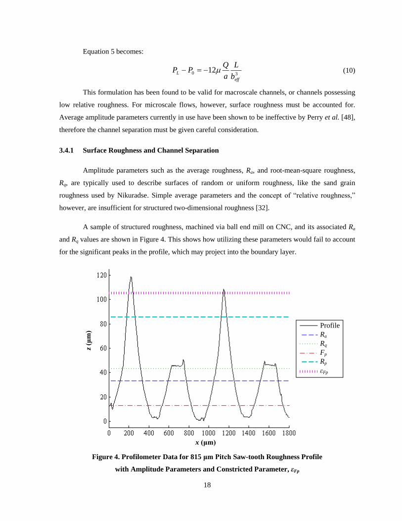
A sample of structured roughness, machined via ball end mill on CNC, and its associated Ra
and Rq values are shown in Figure 4. This shows how utilizing these parameters would fail to account
for the significant peaks in the profile, which may project into the boundary layer.
Figure 4. Profilometer Data for 815 μm Pitch Saw-tooth Roughness Profile
with Amplitude Parameters and Constricted Parameter, εFp
Profile
Ra
Rq
Fp
Rp
εFp
x (μm)
z (μ
m)

19
Kandlikar et al. [3] set forth a method for assessing a surface of significant random roughness
or structured roughness. This new roughness factor, referred to as the constricted flow parameter, is a
function of the average parameters typically obtained through surface analysis:
pa
ppFp
FR
FR
-Max
(11)
where Max is the single highest point obtained from one evaluation length of any given profile. The
floor profile, Fp, also called FdRa, is defined as the average of all points below the mean line, Ra,
which is simply the arithmetic mean of the height of all points along a profile. These additional values
for the 815 μm surface are also shown in Figure 4.
Figure 5. Representative Channel and Roughness
Geometry; h = 100 μm, λ = 400 μm, b = 400 μm
The constricted parameter was used to develop a constricted channel separation bcf for use in
place of beff in equation 10. This constricted separation is calculated as:
Fpcf bb 2 (12)
where b is the root separation between two rough walls, measured between the floor profiles (Fp) of
opposing surfaces. By this definition, any amplitude parameter could be used to “constrict” the
channel separation. Figure 5 shows a sample cross-section of a channel possessing the ideal
Profile
Ra
εFp
x (μm)
z (μ
m)

20
sinusoidal structured roughness discussed previously, with its constricted separation and average
roughness separation. In this figure, it can be seen that using the average roughness to define the
channel separation does not entirely account for the peaks.
In previous studies [45, 46], the constricted parameter was successfully used to fit
experimental data to conventional laminar theory by using the constricted separation bcf in place of
beff, in equation 10. This constricted flow method is effective in accounting for natural or random
roughness, as well as some forms of structured roughness. It is not a strong function of roughness
pitch, however, which is an aspect of structured roughness that is known to have a significant effect
on fluid flow. Nor does the constricted parameter account for shape or alignment of roughness peaks.
Therefore, to improve the understanding of the effects of structured two-dimensional roughness, it
becomes necessary to consider all aspects of roughness geometry by representing the wall roughness
as an exact function of x.
3.5 Further Theoretical Analysis
For relatively high Reynolds numbers, flow can be divided into a bulk region of inviscid flow
unaffected by viscosity, and a region close to the wall where viscosity is significant (the boundary
layer). The inertial term in the x-component of the N-S equation may be non-negligible. This further
analysis allows us to understand the impact of the lubrication approximation itself without the added
complication of unknown velocity profile assumptions. Also, it allows for examination of the velocity
profile from the boundary layer solution and the behavior of the inertial term as the velocity increases
and hydraulic diameter decreases.
An augmented velocity profile is required for this analysis. Incorporating the differential
pressure function from the prior analysis (equation 4) into the initial velocity profile approximation
(equation 2) yields:
)()()()(
63
xfzxgzxfxga
Qu
(13)
In this equation, velocity is strictly a function of flow rate and wall geometry, and varies with
x and z. The profile is parabolic and the equation satisfies the boundary conditions and continuity
equation.

21
Using an augmented lubrication approximation in which the inertial term is not neglected, the
x-component of N-S equation is:
z
uw
x
uu
z
u
x
P
2
2
(14)
Through the use of u-substitution and Leibniz Rule, this differential equation simplifies to:
)(
)(
2
)(
)(
)()(
xg
xf
xg
xf
zuxz
uxfxg
x
P (15)
If the velocity profile is known, this equation may be solved for a pressure–flow relation that
includes the inertial term. Therefore, we use the velocity profile developed previously (equation 13)
as a trial function, yielding the following pressure-drop equation:
LL
L xxfxg
x
xf
x
xg
a
Qx
xfxga
QPP
0
32
2
0
30)()(
)()(
5
6
)()(
112 (16)
The first term of this equation is the same as the previous analysis (equation 5). The inertial
integral is not trivial to solve, however, once the trigonometric profile (equation 6) is applied.
Examining the limits of this analysis can indicate the potential usefulness of this augmented analysis.
If inertia were negligible, as with low Reynolds number flows, this formulation would limit back to
the lubrication approximation equation (equation 5). Similarly, in the smooth wall case, f(x) and g(x)
are constants, the derivatives of which are zero. The inertial integral will then yield a negligible
constant. Thus, the formulation is consistent with the boundary layer analysis for the case of
hydraulically smooth walls. Overall, these limits indicate that the analysis has potential as an
improvement upon the initial analysis, and may be a starting point for future work.

22
3.6 Application of Theory
In order to test the theoretical pressure loss equation (equation 5) and to compare it with
existing laminar flow models, friction factors must be evaluated for varying Reynolds numbers. To
this end, the pressure-loss form of the Darcy-Weisbach equation, or Darcy friction factor, was used to
calculate experimental friction factors:
2
2
A
QD
L
Pf h
(17)
where Dh is the hydraulic diameter, calculated as four times the cross-sectional area divided by the
wetted perimeter:
ba
abDh
2 (18)
The Darcy-Weisbach equation was also used to calculate theoretical friction factors with ΔP
obtained from the wall function method. For comparison with conventional laminar theory, the
correlation for friction factors in smooth, rectangular ducts, from Kakaç et al. [51], was also
evaluated:
)2537.09564.07012.19467.13553.11(Re
24 5432 f (19)
where the aspect ratio is calculated as the channel width divided by channel height:
a
b (20)
Reynolds number was calculated as:
A
QDh
Re (21)
The hydraulic diameter and cross-sectional area may be “constricted” by using the constricted
separation in place of the root separation. Similarly, Reynolds number may be constricted by using
the constricted hydraulic diameter and area. Constricted friction factors may be calculated by using
constricted geometry, as well as the constricted form of equation 10 for pressure drop.

23
4 Preliminary Results
This chapter presents the results of comparison of available data with the theoretical model,
prior to the design and manufacture of a new test set and roughness pieces. In addition, the roughness
profile, equation 6, was evaluated in order to optimize the profile and understand the effects of each
variable on roughness amplitude parameters.
4.1 Saw-tooth Roughness
Experimental data from previous tests by Brackbill [44] were used for comparison with the
wall function method detailed above. Initial validation of the experimental setup was reported for the
hydraulically smooth channel case. Channel separation values were 200, 300, and 500 μm. Flow rates
in these experiments were varied to cover the range of Reynolds numbers from 487 to 2322. Friction
factors were calculated by Brackbill using equation 19 for laminar theory and the constricted Darcy
friction factor for experimental values. Figure 6 shows the comparison between Brackbill‟s
experimental data for hydraulically smooth channels and the smooth channel correlation (Equation
19). For each of these three channel separations, error was less than 4% at all flow rates.
Figure 6. Smooth Channel Validation of Previous Experimental Setup
Laminar Theory
bcf = 200 μm
bcf = 300 μm
bcf = 500 μm
Re
f

24
The style of two-dimensional roughness examined by Brackbill is referred to as “saw-tooth”
roughness. The surfaces possessed evenly spaced peaks, and were described by the roughness height
and pitch. A sample of profilometer data from one such saw-tooth surface is shown in Figure 7 below.
This surface would form one wall of a channel, as shown in Figure 5.
Figure 7. Saw-tooth Roughness Profile with Height Parameters, λ = 503 μm
This figure includes the standard average amplitude parameters, Ra and Rq, as well as the
constricted parameter εFp and its components, Rp and Fp, obtained from the profilometer data. It is
shown that of all these parameters, none fully account for the peak heights, though the constricted
parameter is closest. The peaks for this surface were designed to be 50 µm tall, but the constricted
parameter was found to be 38.75 µm. Amplitude parameters do not account for the distance between
the major peaks, so it becomes necessary to use spatial parameters. However, due to the smaller peaks
between those major peaks, on the order of 20 µm tall, the standard spatial parameters were incapable
of characterizing the major peaks. The roughness between the major peaks has the added effect of
skewing height parameters and complicating the measurement of the root channel separation.
In order to apply the wall function method, the “saw-tooth” surfaces were fit with smooth,
continuous polynomials. This was achieved by examining the profiles and formulating sinusoidal
Profile
Ra
Rq
Fp
Rp
εFp
x (μm)
z (μ
m)

25
functions that fit the curvature. Through a series of curve-fitting exercises, initially using complex
combinations of trigonometric functions, it was quickly determined that the minor peaks could not be
accounted for by any continuous stable function, and so equation 6 was developed. Leaving all
coefficients as variables, the least sum of squares method was used in conjunction with Excel‟s
Solver tool to obtain a best fit. A sample image of the same profilometer data shown in Figure 7 and
its corresponding curve-fit are shown below in Figure 8.
Figure 8. Curve Fit of 503 μm Pitch Saw-tooth Roughness Profile
Figure 8 is one example of a smooth curve of the form of equation 6 (shown in orange) fit to
profilometer data from saw-tooth roughness (shown in black). The height obtained for the curve fit of
this profile is 37.2 µm and the pitch is 416.7 µm. The “floor” of the profile was taken to be the same
as the Fp parameter, shown in Figure 7, but was allowed to vary slightly in order to obtain a best fit.
Although the difference between the curve fit and the surface data was minimized, it is clear that it
does not provide a perfect fit as it neglects the roughness in the valleys between the major peaks. This
minor roughness may be non-negligible in microscale flows, particularly considering interactive flow.
Though the curve does not provide an exact fit, the friction factors obtained through the wall
function method provided an excellent prediction of the channel‟s hydraulic performance for two
channel separations. The two figures below show the un-constricted laminar experimental data
x (μm)
z (μ
m)
Profile
Fit

26
obtained by Brackbill [44] for two channel separations of the 503 µm pitch surface; b = 300 and 400
µm. The plots include the conventional laminar theory line (equation 19), and the line predicted by
the wall function method based on the curve fit of Figure 8.
Figure 9. f vs. Re for 503 μm Pitch Surface, b = 400 μm
Figure 10. f vs. Re for 503 μm Pitch Surface, b = 300 μm
Re
f
Re
f Laminar Theory
Experimental Data
Wall Function
Re
f
Laminar Theory
Experimental Data
Wall Function
27
The experimental data for b = 300 µm are an average of 76% greater than the friction factors
predicted by laminar theory, and for b = 400 µm about 65% greater. The data fits the lines predicted
by the wall function method to within 4% for b = 300 µm and within 10% for b = 400 µm. However,
the wall function method under-predicts the 400µm channel size case and over-predicts the 300 µm.
This may be due, in part, to the roughness between peaks, discussed previously.
Other surfaces were measured, fitted with polynomials, and compared with the wall function
method, but none compared as well as the 503 µm pitch surface. This was due to the increase in
roughness between peaks as the pitch increased. The minor roughness made it difficult to identify the
floor of the profile and thus the root channel separation. It also had the effect of skewing amplitude
parameters so that they were significantly lower than the actual peak height. The overall effect of this
minor roughness on the flow data obtained by Brackbill is unknown.
It should be noted that the wall function method was developed based on the lubrication, or
small-slope approximation, which implies that the slope of the roughness at any point is small. The
profile shown previously clearly does not fit this category. The limits of the lubrication approximation
were tested not only by increasing the roughness height but also by the inclusion of minor roughness
in between the major peaks. In order to properly validate the theoretical model defined herein,
surfaces were designed and manufactured to fit precisely to the power sinusoid of equation 6.
4.2 Idealized Roughness
Before using the wall function method to assess flow in the presence of idealized structured
roughness, the roughness profiles themselves were analyzed numerically in order to understand the
effect of pitch and height on certain amplitude parameters. Equation 6 was studied by systematically
varying each variable and evaluating the effect on the average roughness Ra and RMS roughness Rq,
as well as the constricted parameter εFp and its components, Fp and Rp. For reference, Figure 5 shows
a sample of the roughness studied in this section.
Initially, the height of roughness elements was maintained at h = 50 μm and pitch was varied
such that λ/h ranged from 2 to 12, in order to envelop the “transitional” roughness identified by
Coleman et al. [37]. It was immediately apparent that if the power on the sinusoid was not varied as
well, the slope of the peaks became shallower as pitch increased. The result was that all roughness
parameters remained approximately constant, varying by no more than half a micron, when the height
28
and power were held constant and pitch was varied. This indicated that the existing parameters are
very weak functions of roughness pitch, but may be strongly affected by the power or slope of peaks.
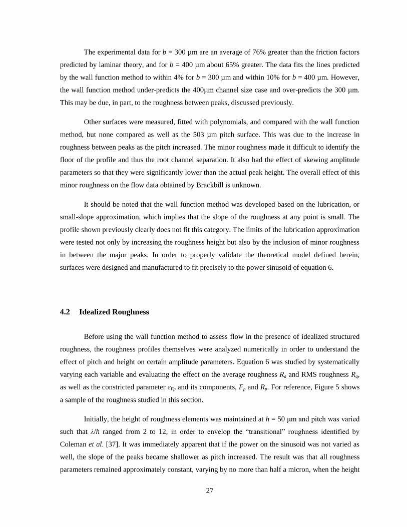
The study was repeated for a constant pitch of 250 µm, keeping the power constant and varying the
height such that λ/h ranged from 2 to 12 once again. The results are shown in Figure 11 below.
Figure 11. Roughness Parameters vs. λ/h for λ = 250 μm and p = 6
As the roughness height decreased, all parameters decreased asymptotically. This is to be
expected for amplitude parameters, as they are direct functions of roughness height. Note that for this
style of idealized roughness, there is very little difference between the constricted parameter and peak
height Rp. This is due to the smoothness of the profile between the peaks, evidenced by the low Fp
value.
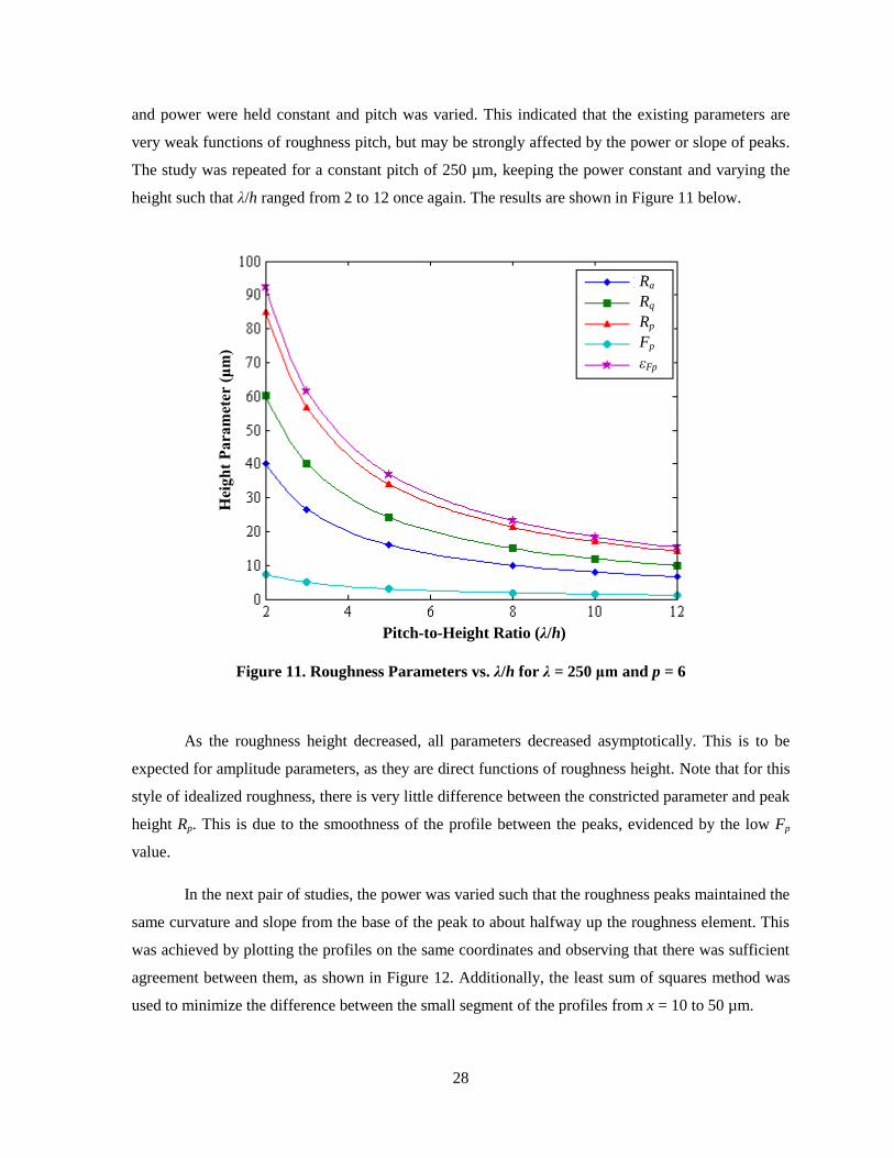
In the next pair of studies, the power was varied such that the roughness peaks maintained the
same curvature and slope from the base of the peak to about halfway up the roughness element. This
was achieved by plotting the profiles on the same coordinates and observing that there was sufficient
agreement between them, as shown in Figure 12. Additionally, the least sum of squares method was
used to minimize the difference between the small segment of the profiles from x = 10 to 50 µm.
Ra
Rq
Rp
Fp
εFp
Pitch-to-Height Ratio (λ/h)
Hei
gh
t P
ara
met
er (
μm
)

29
Figure 12. Ideal Surface Roughness Profiles for h = 50 μm, λ varies, p varies
This process of varying the cosine power was applied to a series of profiles with a constant
pitch of λ = 250 µm, varying the height h such that the same pitch-to-height ratios were obtained.
Figure 13 illustrates the effect of varying the power to keep the roughness slope the same.
Figure 13. Roughness Parameters vs. λ/h for λ = 250 μm, p varies
Ra
Rq
Rp
Fp
εFp
Pitch-to-Height Ratio (λ/h)
Hei
gh
t P
ara
met
er (
μm
)
x (μm)
z (μ
m)
λ/h = 3 λ/h = 5 λ/h = 8

30
Comparing Figure 13with Figure 11, the primary effect of maintaining similar roughness
slopes that it decreases the average amplitude parameters and the floor profile, and increase the
constricted and peak height parameters. The constricted parameter and peak height are essentially the
same in this case. In general, the profiles are “cleaner” or more consistent from one to the next, as
was seen in Figure 12, and as evidenced by the minimal floor profile parameter.
In this next study, roughness height was held constant at 50 µm. Pitch was varied as before,
to obtain the same pitch-to-height ratios, and power was varied as described above. A summary of the
roughness values obtained is shown in Figure 14.
Figure 14. Roughness Parameters vs. λ/h for h = 50 μm, p varies
As the roughness pitch increases, the average amplitude parameters Ra and Rq decrease while
the constricted parameter εFp and peak height Rp increase. This is due to the decrease in the density of
asperities on the surface, indicating that the constricted parameter is more sensitive to these extreme
peaks than the exiting average parameters. For smaller pitch-to-height ratios, there is a significant
difference between the constricted parameter and peak height, as the floor profile parameter Fp
increases with peak density (as pitch decreases). But as pitch increases, Fp diminishes, resulting in εFp
and Rp converging toward the designed height of 50 µm.
Ra
Rq
Rp
Fp
εFp
Pitch-to-Height Ratio (λ/h)
Hei
gh
t P
ara
met
er (
μm
)
31
The results of this analysis indicate that, in general, all amplitude parameters investigated are
sensitive to both pitch and height, particularly in the event that the roughness peaks are closely
spaced, or λ/h is small. The sinusoid power also has a strong effect on the cases of closely spaced
roughness. The constricted parameter εFp and peak height Rp are better suited to this style of
structured or transverse rib roughness than are the average parameters Ra and Rq, The average and
RMS roughness may be sufficient, however, in the case of low roughness height and large pitch-to-
height ratio, as seen in Figure 11. The primary point of interest here is that the amplitude parameters
all exhibit asymptotic behavior as pitch, height, and power are varied, in that the parameters limit to
constant values in either λ/h extreme.
In the literature review, it was noted that the λ/h = 8 case is considered “transitional”
roughness, and has been identified as having the greatest effect on fluid flow. For the constricted flow
model, this would imply that the roughness values reach a maximum at λ/h = 8, and decrease on
either side of that point. It is hoped that the wall function method developed here will be an
improvement on conventional theories in that respect.
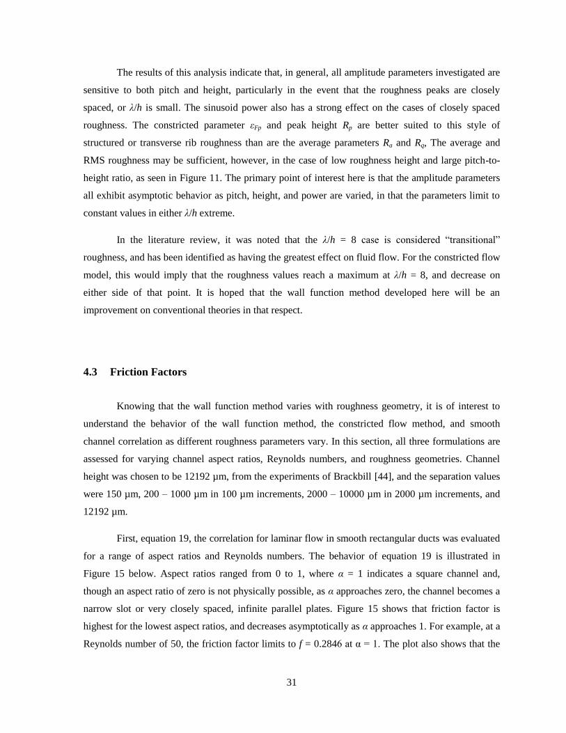
4.3 Friction Factors
Knowing that the wall function method varies with roughness geometry, it is of interest to
understand the behavior of the wall function method, the constricted flow method, and smooth
channel correlation as different roughness parameters vary. In this section, all three formulations are
assessed for varying channel aspect ratios, Reynolds numbers, and roughness geometries. Channel
height was chosen to be 12192 µm, from the experiments of Brackbill [44], and the separation values
were 150 µm, 200 – 1000 µm in 100 µm increments, 2000 – 10000 µm in 2000 µm increments, and
12192 µm.
First, equation 19, the correlation for laminar flow in smooth rectangular ducts was evaluated
for a range of aspect ratios and Reynolds numbers. The behavior of equation 19 is illustrated in
Figure 15 below. Aspect ratios ranged from 0 to 1, where α = 1 indicates a square channel and,
though an aspect ratio of zero is not physically possible, as α approaches zero, the channel becomes a
narrow slot or very closely spaced, infinite parallel plates. Figure 15 shows that friction factor is
highest for the lowest aspect ratios, and decreases asymptotically as α approaches 1. For example, at a
Reynolds number of 50, the friction factor limits to f = 0.2846 at α = 1. The plot also shows that the
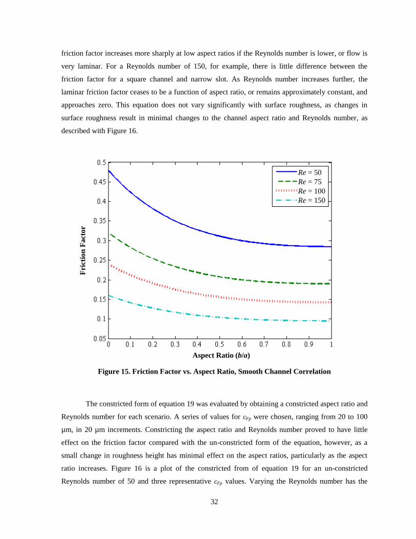
32
friction factor increases more sharply at low aspect ratios if the Reynolds number is lower, or flow is
very laminar. For a Reynolds number of 150, for example, there is little difference between the
friction factor for a square channel and narrow slot. As Reynolds number increases further, the
laminar friction factor ceases to be a function of aspect ratio, or remains approximately constant, and
approaches zero. This equation does not vary significantly with surface roughness, as changes in
surface roughness result in minimal changes to the channel aspect ratio and Reynolds number, as
described with Figure 16.
Figure 15. Friction Factor vs. Aspect Ratio, Smooth Channel Correlation
The constricted form of equation 19 was evaluated by obtaining a constricted aspect ratio and
Reynolds number for each scenario. A series of values for εFp were chosen, ranging from 20 to 100
µm, in 20 µm increments. Constricting the aspect ratio and Reynolds number proved to have little
effect on the friction factor compared with the un-constricted form of the equation, however, as a
small change in roughness height has minimal effect on the aspect ratios, particularly as the aspect
ratio increases. Figure 16 is a plot of the constricted from of equation 19 for an un-constricted
Reynolds number of 50 and three representative εFp values. Varying the Reynolds number has the
Re = 50
Re = 75
Re = 100
Re = 150
Aspect Ratio (b/a)
Fri
ctio
n F
act
or

33
same effect as seen in Figure 15, thus only one Reynolds number is shown in Figure 16, so as to
highlight the effect of varying εFp.
Figure 16. Friction Factor vs. Aspect Ratio, Constricted Flow Method, Re = 50
As illustrated by Figure 16 above, the friction factor lines for varying roughness heights differ
very slightly for narrow channels. The difference between fiction factors for εFp = 20 and 100 μm, for
example, is approximately 1.6% for small aspect ratios and decreases to 0.7% as α approaches 1.
Percent error between the constricted and un-constricted forms of equation 19 was found to be about
0.2% at low aspect ratios, and decreased to zero as aspect ratio increased, for all εFp. For this reason,
the un-constricted laminar friction factor (equation 19) was used for further comparison in the study
of the wall function method, and for comparison with experimental data.
To assess the behavior of friction factors obtained from the wall function method, idealized
surfaces based on equation 6, identical to those shown in Figure 12, were modeled with a constant
height of h = 50 µm. The roughness pitches modeled were λ = 100, 150, 250, 400, 500, and 600 µm.
The corresponding pitch-to-height ratios for these surfaces are λ/h = 2, 3, 5, 8, 10, and 12. The cosine
power was varied, as described in the Idealized Roughness section, so that the slope was relatively
εFp = 20
εFp = 60
εFp = 100
Aspect Ratio (b/a)
Fri
ctio
n F
act
or

34
constant across all profiles. These wall function variables were entered into the MATLAB code,
shown in Appendix A. Fluid density and viscosity were held constant for all simulations. Reynolds
number was used for the input parameter associated with flow rate in this version of the code, and the
volumetric flow rate was calculated based on channel geometry, fluid properties, and Reynolds
number. For this analysis, Reynolds number was set to 50, and channel separations ranged from 150
to 12192, as described at the beginning of this section. The evaluation length was set to 1.0 inch, to
match the distance between pressure taps in prior experiments. The theoretical pressure drop was
evaluated in MATLAB using equation 5 and the wall functions, equation 6. The pressure drop was
then incorporated into equation 17 for friction factor. The results of this exercise are plotted on a log-
log graph, in Figure 17 below, in order to magnify the behavior of wall function friction factors in the
low aspect ratio range.
Figure 17. Friction Factor vs. Aspect Ratio, Wall Function Method, Re = 50
The “Smooth” line shown in Figure 17 was calculated using equation 19, and is the same as
the line plotted in Figure 15 for Re = 50. This line was plotted for smooth channel comparison
because the wall functions studied here were for a constant roughness height. It was found that setting
Smooth
λ/h = 2
λ/h = 3
λ/h = 5
λ/h = 8
λ/h = 10
λ/h = 12
Aspect Ratio (b/a)
Fri
ctio
n F
act
or

35
the wall functions f(x) and g(x) to constant values, or setting h = 0, resulted in friction factors within
1.2% of smooth channel theory.
This plot is intended to display the comparative behavior of the wall function method and the
smooth channel correlation. Like the smooth channel correlation, the friction factors predicted by the
wall function method decrease as Reynolds number increases, as discussed previously for Figure 15.
At the low end of aspect ratios, both theories predict higher friction factors, so they agree that friction
factor is greater in taller/narrower channels. The roughness height was held constant for this study,
and the small pitch-to-height ratios indicate very closely spaced roughness, for which the wall
function method predicts very high friction factors. As roughness spacing increases on the low
channel aspect ratio end, the wall function method appears to converge toward the smooth channel
correlation (see λ/h = 10 and 12 in Figure 17). As channel aspect ratio increases toward a square
channel, the wall function decreases asymptotically to a friction factor of 0.5 for all roughness
profiles. This is higher than the smooth channel correlation predicted, but the value decreases towards
the smooth channel correlation as roughness height decreases. This view of the wall function
method‟s behavior may be indicative of its range of applicability, and in fact reinforces the theoretical
methods used to obtain this theory, as one of the assumptions for the analysis was that the channel
separation is significantly less than the channel height.
In the range of lower channel aspect ratios and higher roughness pitch-to-height ratios, the
wall function method exhibits some instability. The friction factor lines for the three pitch-to-height
values λ/h = 8, 10, and 12 are nearly indistinguishable, and in fact the λ/h = 12 profile resulted in
friction factors greater than the λ/h = 10 surface for the smallest three aspect ratios modeled. As
Reynolds number varies, this instability neither increases nor diminishes. The instability may be due,
in part, to the increase in cosine power as roughness pitch increases. High pitch-to-height ratios are
representative of low relative roughness, so the instability in this range may indicate that the wall
function method will be less accurate as roughness decreases and the user should revert to the
conventional smooth channel correlation.
In addition to the wall function method, the constricted flow method was used in predicting
hydraulic performance for each of these scenarios. The code in Appendix A includes the constricted
flow approach at the end, with the added ability to switch between using the constricted flow
parameter or average roughness for the analysis. It was hoped that evaluating the constricted pressure
drop would provide some improvement over the constricted form of equation 19. The results of the
constricted flow analysis showed that this method is incapable of predicting friction factors that differ
36
from the smooth channel correlation, as was discussed with Figure 16. The greatest difference
observed between the constricted flow method and the equation for smooth channels was, as the
channel separation increased, the friction factors obtained from the constricted flow method became
increasingly lower than those predicted by the smooth channel correlation.
The overall outcome of this systematic study of friction factor behavior is that the wall
function method appears to be most effective in the case of low channel aspect ratios and low
roughness pitch-to-height ratios. Above channel aspect ratios of 0.1, friction factors obtained from the
wall function method converge to a value much higher than predicted by the smooth channel
correlation. But, as channel size increases, the roughness effect on flow is expected to diminish. The
same is true for high roughness pitch-to-height ratios, in that the sparse roughness elements result in
flow over independent obstructions rather than through a rough channel. Therefore, it was concluded
that further work on the wall function method shall be focused on smaller channel separations and
lower roughness pitch-to-height ratios.
4.4 Flow through Channels Possessing Idealized Roughness
Analysis of flow in the presence of the two-dimensional roughness was performed on the
same idealized surfaces discussed in the previous section. The format of equation 6 was used for the
wall functions, where h was held at a constant value of 50 μm, and λ was varied such that λ/h = 3, 5,
8, and 10. The root channel separation values modeled were 150 μm, and 200-600 μm in 100 μm
increments. Channel height was fixed at 12192 µm, as before. Reynolds number ranged from 5 to
3400. All roughness parameters for these theoretical surfaces were calculated in the roughness
analysis performed prior. The range of profiles and channel separations resulted in relative roughness
values, εFp/Dh, ranging from 3-15%.
For a constant channel separation, as λ/h increases (or relative roughness decreases) the wall
function method converges toward laminar theory for smooth rectangular ducts. An example of this
convergence can be seen in Figure 18, which shows friction factors versus Reynolds number for each
surface modeled, when channel separation was held constant at 150 μm. The smooth channel
correlation, shown in black, was calculated using equation 19. Higher values of λ/h indicate lower
roughness effect on fluid flow, in that the peaks become isolated flow obstructions rather than
periodic roughness, eventually limiting to the hydraulically smooth case. As roughness pitch

37
decreases, the increase in friction factor is more pronounced, as seen in the differences between the
“Smooth” line and λ/h = 3 and = 5.
Figure 18. Comparison of Wall Function Method with Smooth Channel
Correlation, for Channel Separation b = 150 μm
Figure 19 shows a plot of friction factor versus Reynolds number for a single surface, λ/h = 5,
and four different channel separations; b = 150, 200, 300, and 500 µm. For any given roughness
profile, as the channel separation increases from microscale to macroscale, the wall function method
again converges to the smooth channel correlation for rectangular ducts. This is because microscale
roughness has minimal effect on the bulk flow in larger scale channels [36]. In these cases, aspect
ratio increases minutely with the increase of separation from 150 μm to 600 μm, because the channel
height is significantly greater than the width, and so the corresponding decrease in the smooth
channel friction factor is 1.2%. The smooth correlation lines in Figures 18 and 19 correspond with the
150 µm channel separation.
Smooth
λ/h = 3
λ/h = 5
λ/h = 8
λ/h = 10
Re
f

38
Figure 19. Comparison of Wall Function Method with Smooth Channel
Correlation, for Surface Profile λ/h = 5
In general, it was shown using the wall function method that for larger hydraulic diameters
and larger λ/h ratios, i.e., lower relative roughness (εFp/Dh < 5%), the friction factor deviates little
from the correlation for laminar flow in smooth rectangular ducts. As the channel separation
decreases, the roughness height becomes of the same order of the channel separation, resulting in a
significant increase in roughness effect, evident in the plots discussed previously. For large roughness
pitch values, this effect is not evident until the ratio of roughness height to channel separation h/b is at
least 0.25. For lower values of λ/h, the difference between the wall function method and laminar
theory is significant for h/b ≈ 0.08.
Smooth
λ/h = 3
λ/h = 5
λ/h = 8
λ/h = 10
Re
f

39
5 Experimental Setup
In order to assess the validity of the theoretical analysis, and thereby test the limits of the
applied assumptions and approximations, it is necessary to perform experiments with fluid flow in the
roughness and channel geometries studied in the previous sections. Surfaces designed based on
equation 6 were generated in stainless steel and evaluated using a Keyence laser confocal microscope.
A complete experimental apparatus and test loop was also developed for testing. The test components
will be discussed in the following subsections.
5.1 Design Parameters
A universal test matrix was developed to ensure geometric similitude across all experimental,
theoretical, and numerical analyses associated with the project. Summaries of the test matrix for
roughness parameters and channel geometry are shown in Table 1 and Table 2, respectively. The
complete design test matrix, as it applies to this work, can be found in Appendix B.
Table 1. Test Matrix Summary: Roughness Geometry - Designed
Pitch Height Power Pitch-to-
Height Ratio
λ h p λ/h
μm μm --- ---
250 125 4 2
150 50 4 3
250 50 12 5
250 31.25 4 8
400 50 32 8
Table 2. Test Matrix Summary: Channel Geometry - Designed
Separation Hydraulic
Diameter
Aspect
Ratio
Separation-
to-Length
Ratio
b Dh α b/L
μm μm --- ---
250 480 0.02 0.002
450 850 0.04 0.003
600 1118 0.05 0.004
800 1600 0.06 0.005
1000 1964 0.08 0.007
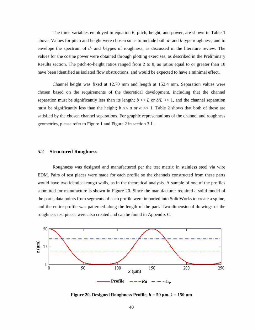
40
The three variables employed in equation 6, pitch, height, and power, are shown in Table 1
above. Values for pitch and height were chosen so as to include both d- and k-type roughness, and to
envelope the spectrum of d- and k-types of roughness, as discussed in the literature review. The
values for the cosine power were obtained through plotting exercises, as described in the Preliminary
Results section. The pitch-to-height ratios ranged from 2 to 8, as ratios equal to or greater than 10
have been identified as isolated flow obstructions, and would be expected to have a minimal effect.
Channel height was fixed at 12.70 mm and length at 152.4 mm. Separation values were
chosen based on the requirements of the theoretical development, including that the channel
separation must be significantly less than its length; b << L or b/L << 1, and the channel separation
must be significantly less than the height; b << a or α << 1. Table 2 shows that both of these are
satisfied by the chosen channel separations. For graphic representations of the channel and roughness
geometries, please refer to Figure 1 and Figure 2 in section 3.1.
5.2 Structured Roughness
Roughness was designed and manufactured per the test matrix in stainless steel via wire
EDM. Pairs of test pieces were made for each profile so the channels constructed from these parts
would have two identical rough walls, as in the theoretical analysis. A sample of one of the profiles
submitted for manufacture is shown in Figure 20. Since the manufacturer required a solid model of
the parts, data points from segments of each profile were imported into SolidWorks to create a spline,
and the entire profile was patterned along the length of the part. Two-dimensional drawings of the
roughness test pieces were also created and can be found in Appendix C.
Figure 20. Designed Roughness Profile, h = 50 μm, λ = 150 μm
x (μm)
z (μ
m)
Profile Ra εFp

41
The method of wire EDM was chosen based on the need for precise patterning on the
roughness test pieces, and the complex shape of the gauge blocks (discussed later). One of the
drawbacks to this method was the size of wire used in the process, 101.6 µm, which limited the
minimum roughness pitch allowable. Another difficulty was the severe deformation of the initial
batch of roughness pieces. This was prevented in the second and subsequent batches by stress-
relieving the steel plate from which the parts were cut.
Once the test pieces were obtained, they were cleaned by rinsing with methanol, acetone,
IPA, and water sequentially, blowing the surfaces dry with compressed air between rinses. Multiple
sample lengths of each surface were then scanned on the laser confocal microscope, which has a
resolution of 1 nm. A total of 5 scans were taken for each test piece, or 10 scans per roughness
profile, at even and consistent intervals. A sample 3-D image result from the microscope is shown in
Figure 21. This surface was manufactured from the submitted profile show previously in Figure 20.
Figure 21. Laser Confocal Image of Wire EDM Result, Rstep = 49.6 μm, RSM = 149.8 μm
Roughness parameters were obtained from each scan and averaged for each profile. The
roughness parameters of interest, set forth in Table 3 below, were determined based on information
found in literature and through assessment of the profile described by equation 6. Some, if not all, of
these parameters were expected to correlate with the variables in equation 6. In particular, the
amplitude parameters were expected to correlate with the height h, and the spatial parameters would
correlate with the pitch λ. The remaining parameters were hoped to correlate with the roughness
slope, or cosine power p. These parameters have all been noted in literature and were evaluated to
determine their relevance. Results from the surface scans can be found in Table 8 in the Results
section.
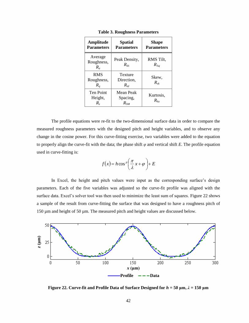
42
Table 3. Roughness Parameters
Amplitude
Parameters
Spatial
Parameters
Shape
Parameters
Average
Roughness,
Ra
Peak Density,
Rds
RMS Tilt,
RΔq
RMS
Roughness,
Rq
Texture
Direction,
Rtd
Skew,
Rsk
Ten Point
Height,
Rz
Mean Peak
Spacing,
RSM
Kurtosis,
Rku
The profile equations were re-fit to the two-dimensional surface data in order to compare the
measured roughness parameters with the designed pitch and height variables, and to observe any
change in the cosine power. For this curve-fitting exercise, two variables were added to the equation
to properly align the curve-fit with the data; the phase shift φ and vertical shift E. The profile equation
used in curve-fitting is:
Exhxf p
cos
In Excel, the height and pitch values were input as the corresponding surface‟s design
parameters. Each of the five variables was adjusted so the curve-fit profile was aligned with the
surface data. Excel‟s solver tool was then used to minimize the least sum of squares. Figure 22 shows
a sample of the result from curve-fitting the surface that was designed to have a roughness pitch of
150 µm and height of 50 µm. The measured pitch and height values are discussed below.
Figure 22. Curve-fit and Profile Data of Surface Designed for h = 50 μm, λ = 150 μm
x (μm)
z (μ
m)
Profile Data
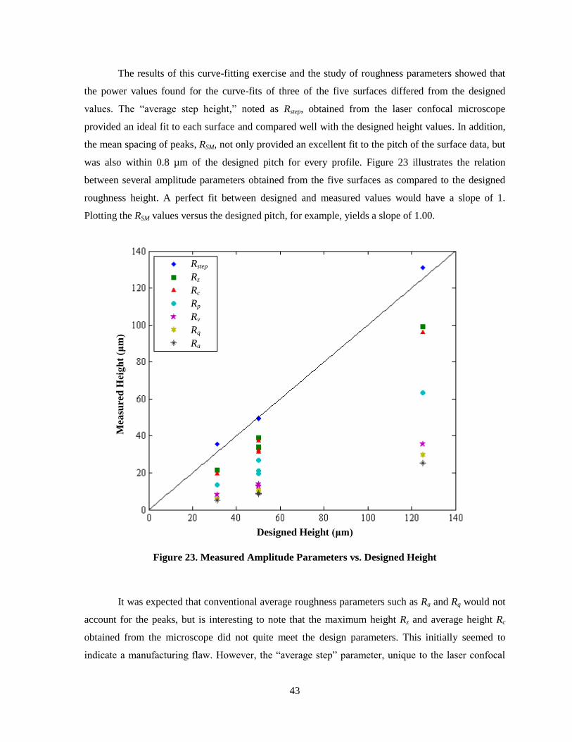
43
The results of this curve-fitting exercise and the study of roughness parameters showed that
the power values found for the curve-fits of three of the five surfaces differed from the designed
values. The “average step height,” noted as Rstep, obtained from the laser confocal microscope
provided an ideal fit to each surface and compared well with the designed height values. In addition,
the mean spacing of peaks, RSM, not only provided an excellent fit to the pitch of the surface data, but
was also within 0.8 µm of the designed pitch for every profile. Figure 23 illustrates the relation
between several amplitude parameters obtained from the five surfaces as compared to the designed
roughness height. A perfect fit between designed and measured values would have a slope of 1.
Plotting the RSM values versus the designed pitch, for example, yields a slope of 1.00.
Figure 23. Measured Amplitude Parameters vs. Designed Height
It was expected that conventional average roughness parameters such as Ra and Rq would not
account for the peaks, but is interesting to note that the maximum height Rz and average height Rc
obtained from the microscope did not quite meet the design parameters. This initially seemed to
indicate a manufacturing flaw. However, the “average step” parameter, unique to the laser confocal
Rstep
Rz
Rc
Rp
Rv
Rq
Ra
Designed Height (μm)
Mea
sure
d H
eigh
t (μ
m)
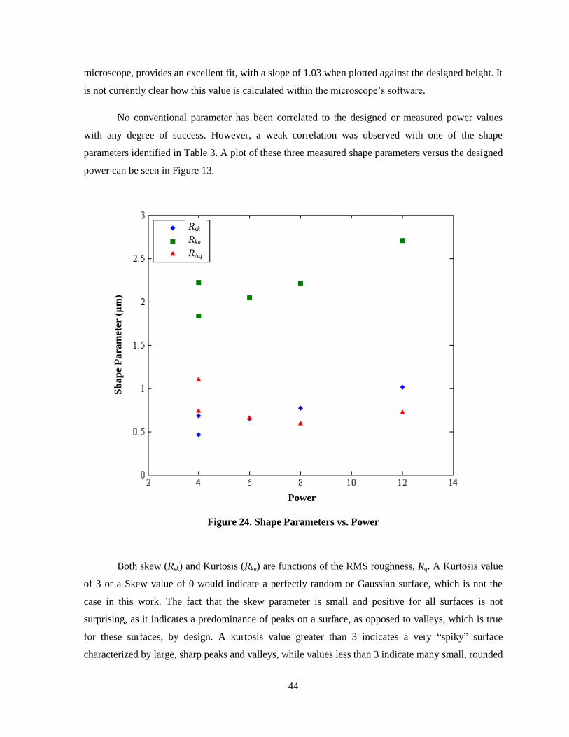
44
microscope, provides an excellent fit, with a slope of 1.03 when plotted against the designed height. It
is not currently clear how this value is calculated within the microscope‟s software.
No conventional parameter has been correlated to the designed or measured power values
with any degree of success. However, a weak correlation was observed with one of the shape
parameters identified in Table 3. A plot of these three measured shape parameters versus the designed
power can be seen in Figure 13.
Figure 24. Shape Parameters vs. Power
Both skew (Rsk) and Kurtosis (Rku) are functions of the RMS roughness, Rq. A Kurtosis value
of 3 or a Skew value of 0 would indicate a perfectly random or Gaussian surface, which is not the
case in this work. The fact that the skew parameter is small and positive for all surfaces is not
surprising, as it indicates a predominance of peaks on a surface, as opposed to valleys, which is true
for these surfaces, by design. A kurtosis value greater than 3 indicates a very “spiky” surface
characterized by large, sharp peaks and valleys, while values less than 3 indicate many small, rounded
Rsk
Rku
RΔq
Power
Sh
ap
e P
ara
met
er (
μm
)

45
peaks and valleys. RMS slope (RΔq) is the average of slopes at all points, but does not correlate with
any variable for these surfaces. The power value still requires some investigation in order to find a
way to predict or estimate it for different structured surfaces, knowing that as pitch increases, the
power increases non-linearly.
For experimental and theoretical calculations, the roughness profile geometries that were
used were the average step height Rstep and mean spacing of peaks RSM, detailed in Table 8 of the
Results section. The power values were obtained through curve-fitting and visually verifying
agreement between the curve-fit and surface data.
5.3 Channel Assembly
An experimental test set was designed using SolidWorks and machined in the Brinkman Lab.
Figure 25 shows the geometry of the roughness test pieces. The surface labeled “rough face”
possesses the structured roughness detailed previously. Thermocouple holes were drilled to a quarter
of the channel depth for concurrent heat transfer testing.
Figure 25. Solid Model of Roughness Test Piece
Thermocouple holes
Rough face
Heaters adhered
to this side
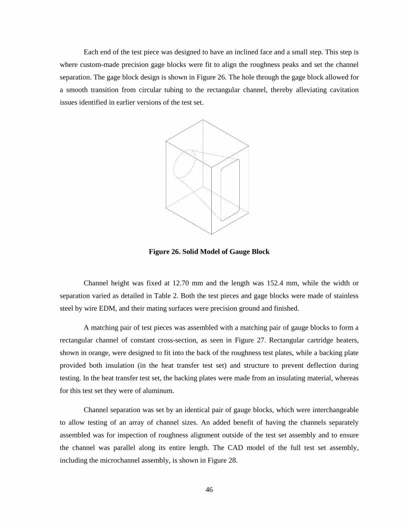
46
Each end of the test piece was designed to have an inclined face and a small step. This step is
where custom-made precision gage blocks were fit to align the roughness peaks and set the channel
separation. The gage block design is shown in Figure 26. The hole through the gage block allowed for
a smooth transition from circular tubing to the rectangular channel, thereby alleviating cavitation
issues identified in earlier versions of the test set.
Figure 26. Solid Model of Gauge Block
Channel height was fixed at 12.70 mm and the length was 152.4 mm, while the width or
separation varied as detailed in Table 2. Both the test pieces and gage blocks were made of stainless
steel by wire EDM, and their mating surfaces were precision ground and finished.
A matching pair of test pieces was assembled with a matching pair of gauge blocks to form a
rectangular channel of constant cross-section, as seen in Figure 27. Rectangular cartridge heaters,
shown in orange, were designed to fit into the back of the roughness test plates, while a backing plate
provided both insulation (in the heat transfer test set) and structure to prevent deflection during
testing. In the heat transfer test set, the backing plates were made from an insulating material, whereas
for this test set they were of aluminum.
Channel separation was set by an identical pair of gauge blocks, which were interchangeable
to allow testing of an array of channel sizes. An added benefit of having the channels separately
assembled was for inspection of roughness alignment outside of the test set assembly and to ensure
the channel was parallel along its entire length. The CAD model of the full test set assembly,
including the microchannel assembly, is shown in Figure 28.
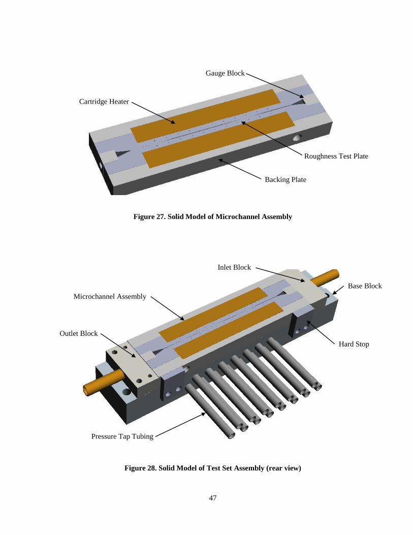
47
Figure 27. Solid Model of Microchannel Assembly
Figure 28. Solid Model of Test Set Assembly (rear view)
Backing Plate
Cartridge Heater
Gauge Block
Roughness Test Plate
Microchannel Assembly
Inlet Block
Hard Stop
Pressure Tap Tubing
Outlet Block
Base Block
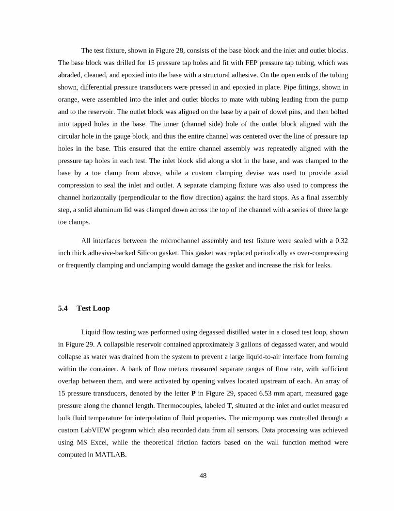
48
The test fixture, shown in Figure 28, consists of the base block and the inlet and outlet blocks.
The base block was drilled for 15 pressure tap holes and fit with FEP pressure tap tubing, which was
abraded, cleaned, and epoxied into the base with a structural adhesive. On the open ends of the tubing
shown, differential pressure transducers were pressed in and epoxied in place. Pipe fittings, shown in
orange, were assembled into the inlet and outlet blocks to mate with tubing leading from the pump
and to the reservoir. The outlet block was aligned on the base by a pair of dowel pins, and then bolted
into tapped holes in the base. The inner (channel side) hole of the outlet block aligned with the
circular hole in the gauge block, and thus the entire channel was centered over the line of pressure tap
holes in the base. This ensured that the entire channel assembly was repeatedly aligned with the
pressure tap holes in each test. The inlet block slid along a slot in the base, and was clamped to the
base by a toe clamp from above, while a custom clamping devise was used to provide axial
compression to seal the inlet and outlet. A separate clamping fixture was also used to compress the
channel horizontally (perpendicular to the flow direction) against the hard stops. As a final assembly
step, a solid aluminum lid was clamped down across the top of the channel with a series of three large
toe clamps.
All interfaces between the microchannel assembly and test fixture were sealed with a 0.32
inch thick adhesive-backed Silicon gasket. This gasket was replaced periodically as over-compressing
or frequently clamping and unclamping would damage the gasket and increase the risk for leaks.
5.4 Test Loop
Liquid flow testing was performed using degassed distilled water in a closed test loop, shown
in Figure 29. A collapsible reservoir contained approximately 3 gallons of degassed water, and would
collapse as water was drained from the system to prevent a large liquid-to-air interface from forming
within the container. A bank of flow meters measured separate ranges of flow rate, with sufficient
overlap between them, and were activated by opening valves located upstream of each. An array of
15 pressure transducers, denoted by the letter P in Figure 29, spaced 6.53 mm apart, measured gage
pressure along the channel length. Thermocouples, labeled T, situated at the inlet and outlet measured
bulk fluid temperature for interpolation of fluid properties. The micropump was controlled through a
custom LabVIEW program which also recorded data from all sensors. Data processing was achieved
using MS Excel, while the theoretical friction factors based on the wall function method were
computed in MATLAB.
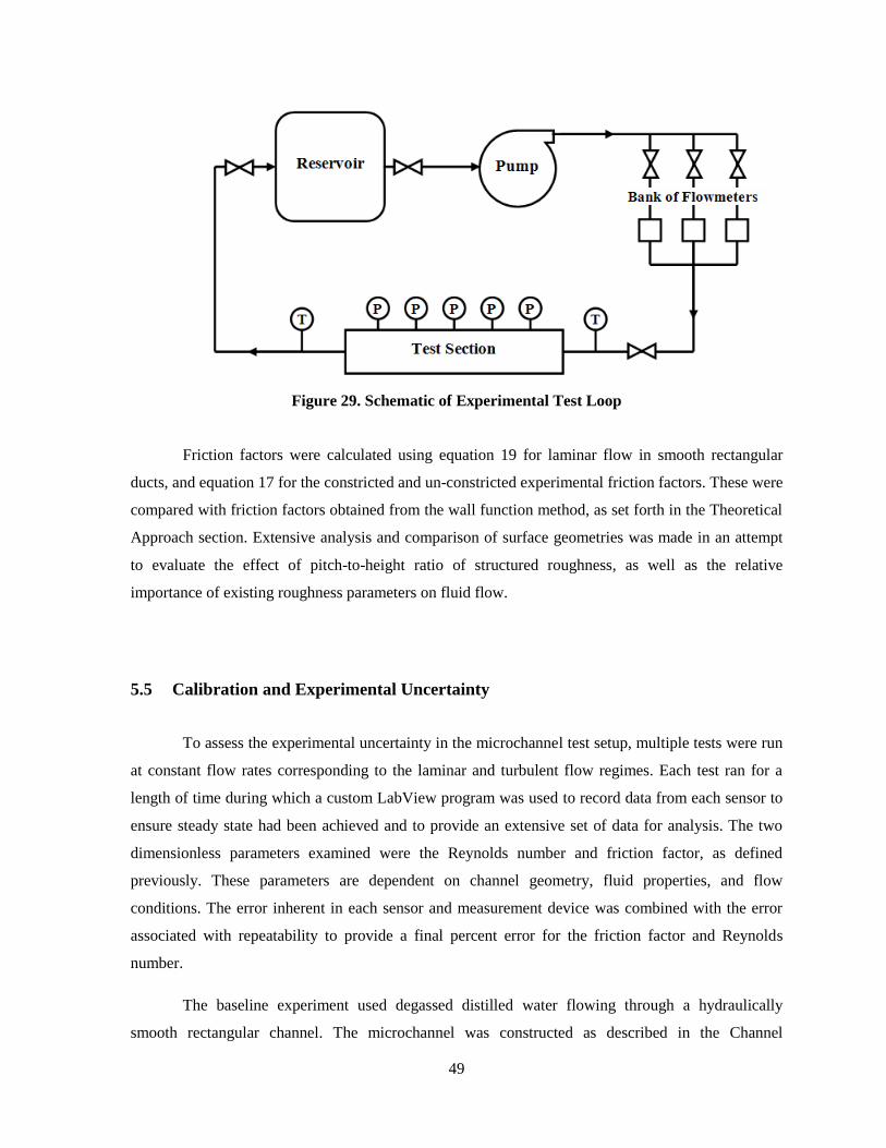
49
Figure 29. Schematic of Experimental Test Loop
Friction factors were calculated using equation 19 for laminar flow in smooth rectangular
ducts, and equation 17 for the constricted and un-constricted experimental friction factors. These were
compared with friction factors obtained from the wall function method, as set forth in the Theoretical
Approach section. Extensive analysis and comparison of surface geometries was made in an attempt
to evaluate the effect of pitch-to-height ratio of structured roughness, as well as the relative
importance of existing roughness parameters on fluid flow.
5.5 Calibration and Experimental Uncertainty
To assess the experimental uncertainty in the microchannel test setup, multiple tests were run
at constant flow rates corresponding to the laminar and turbulent flow regimes. Each test ran for a
length of time during which a custom LabView program was used to record data from each sensor to
ensure steady state had been achieved and to provide an extensive set of data for analysis. The two
dimensionless parameters examined were the Reynolds number and friction factor, as defined
previously. These parameters are dependent on channel geometry, fluid properties, and flow
conditions. The error inherent in each sensor and measurement device was combined with the error
associated with repeatability to provide a final percent error for the friction factor and Reynolds
number.
The baseline experiment used degassed distilled water flowing through a hydraulically
smooth rectangular channel. The microchannel was constructed as described in the Channel
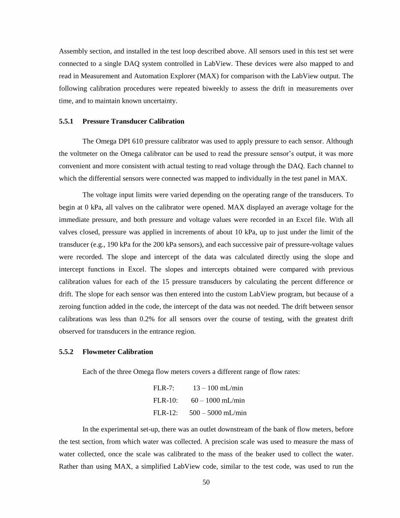
50
Assembly section, and installed in the test loop described above. All sensors used in this test set were
connected to a single DAQ system controlled in LabView. These devices were also mapped to and
read in Measurement and Automation Explorer (MAX) for comparison with the LabView output. The
following calibration procedures were repeated biweekly to assess the drift in measurements over
time, and to maintain known uncertainty.
5.5.1 Pressure Transducer Calibration
The Omega DPI 610 pressure calibrator was used to apply pressure to each sensor. Although
the voltmeter on the Omega calibrator can be used to read the pressure sensor‟s output, it was more
convenient and more consistent with actual testing to read voltage through the DAQ. Each channel to
which the differential sensors were connected was mapped to individually in the test panel in MAX.
The voltage input limits were varied depending on the operating range of the transducers. To
begin at 0 kPa, all valves on the calibrator were opened. MAX displayed an average voltage for the
immediate pressure, and both pressure and voltage values were recorded in an Excel file. With all
valves closed, pressure was applied in increments of about 10 kPa, up to just under the limit of the
transducer (e.g., 190 kPa for the 200 kPa sensors), and each successive pair of pressure-voltage values
were recorded. The slope and intercept of the data was calculated directly using the slope and
intercept functions in Excel. The slopes and intercepts obtained were compared with previous
calibration values for each of the 15 pressure transducers by calculating the percent difference or
drift. The slope for each sensor was then entered into the custom LabView program, but because of a
zeroing function added in the code, the intercept of the data was not needed. The drift between sensor
calibrations was less than 0.2% for all sensors over the course of testing, with the greatest drift
observed for transducers in the entrance region.
5.5.2 Flowmeter Calibration
Each of the three Omega flow meters covers a different range of flow rates:
FLR-7: 13 – 100 mL/min
FLR-10: 60 – 1000 mL/min
FLR-12: 500 – 5000 mL/min
In the experimental set-up, there was an outlet downstream of the bank of flow meters, before
the test section, from which water was collected. A precision scale was used to measure the mass of
water collected, once the scale was calibrated to the mass of the beaker used to collect the water.
Rather than using MAX, a simplified LabView code, similar to the test code, was used to run the

51
pump at a constant RPM, record the time, and to record the voltage output from the flow sensor. Data
was recorded in the Excel calibration file and analyzed similar to the pressure data. Dividing the mass
of water by the time the pump was run provided the mass flow rate. The correlation between the flow
rates and the voltage output from each flowmeter was then implemented in the custom LabView
code.
5.5.3 Thermocouple Calibration
A two-point calibration was sufficient for this experiment, as the thermocouples were used
for interpolation of bulk fluid properties. The two points require an ice bath (0°C) and boiling water
(100°C). Prior to performing this calibration, the thermocouples and containers were cleaned
thoroughly with distilled water.
For the ice bath, the container was filled with shaved or crushed clear ice made from distilled
water. Distilled water was also added to create an ice bath with enough water to provide good thermal
contact with the thermometers, but not so much as to cause the ice to float. A thermometer was kept
in the container and used to stir the ice bath every few minutes to prevent cavities or air pockets from
forming as ice melted. Temperature was allowed to stabilize for about half an hour, while stirring the
ice, draining off excess water, and adding ice as needed. The thermocouples were inserted into the
bath such that they were submerged to the same depth, with at least a few inches of ice between them
and the bottom and sides of the container. It was also ensured that the thermocouples were at the same
depth and not in contact with one another. Temperature values were read from the uncalibrated
thermocouples in LabView over time, and recorded in the Excel file.
The procedure was repeated for boiling water, using a hot plate to bring distilled water to a
boil and inserting the thermocouples to the same depth requirements. The thermocouples were
allowed to reach a steady temperature, which was recorded from Lab View into Excel. A linear
correlation for temperature was implemented into the LabView code as with the pressure transducers.
5.5.4 Bias and Precision Error
There are two classifications of error said to affect system measurements; bias and precision.
Bias, or systematic error, occurs repeatedly with each measurement. It includes calibration, loading,
and resolution errors and is typically reported by the sensor‟s manufacturer as a percentage. Precision,
or random error, is the irregular fluctuation or variance in data, such as white noise, which cannot be
filtered. These errors were assessed for each device used in these experiments.

52
Precision and bias errors may be evaluated analytically by assuming that uncertainties behave
like standard deviations. A specific physical quantity, y can be considered to be a function of the
independent measurements made to obtain its value:
nxxxfy ...,, 21
in which xi represents any individual measurement, where i ranges from 1 to n. Total uncertainty
combines both bias and precision errors through the following formulation:
22
yyy PBU
where By represents bias error and Py represents precision error associated with the measured
quantity, y. Bias error is fairly straightforward to estimate, as it is dependent on the apparent accuracy
of any given sensor, and may be calculated as:
22
2
2
1
2
1
2
...21
n
i
x
n
xx
n
i
x
i
y
Bx
yB
x
yB
x
y
Bx
yB
In the above equation, ixB represents the bias, reported as a percent error by the
manufacturer, associated for the ith instrument used in taking the necessary measurements to obtain xi.
The partial derivative of the physical quantity with respect to a given measurement, ix
y
, represents
the weight which that measurement carries in calculating the physical quantity. This value may be
taken to be the absolute value of the exponent on that variable in the relation nxxxfy ...,, 21 . A
brief study was carried out to assess the difference in calculating the partial derivatives for each
variable, as opposed to taking the partial derivative to be the power of the variable, and it was found
that the percent error is marginally larger when using the power, providing a more conservative
estimate for the error.
Precision error is not expressly given for each device since it is typically related to
unpredictable fluctuations in the data, and is sometimes classified as “human error.” It may be treated
in the same manner as bias error by estimating a standard deviation based on knowledge of the
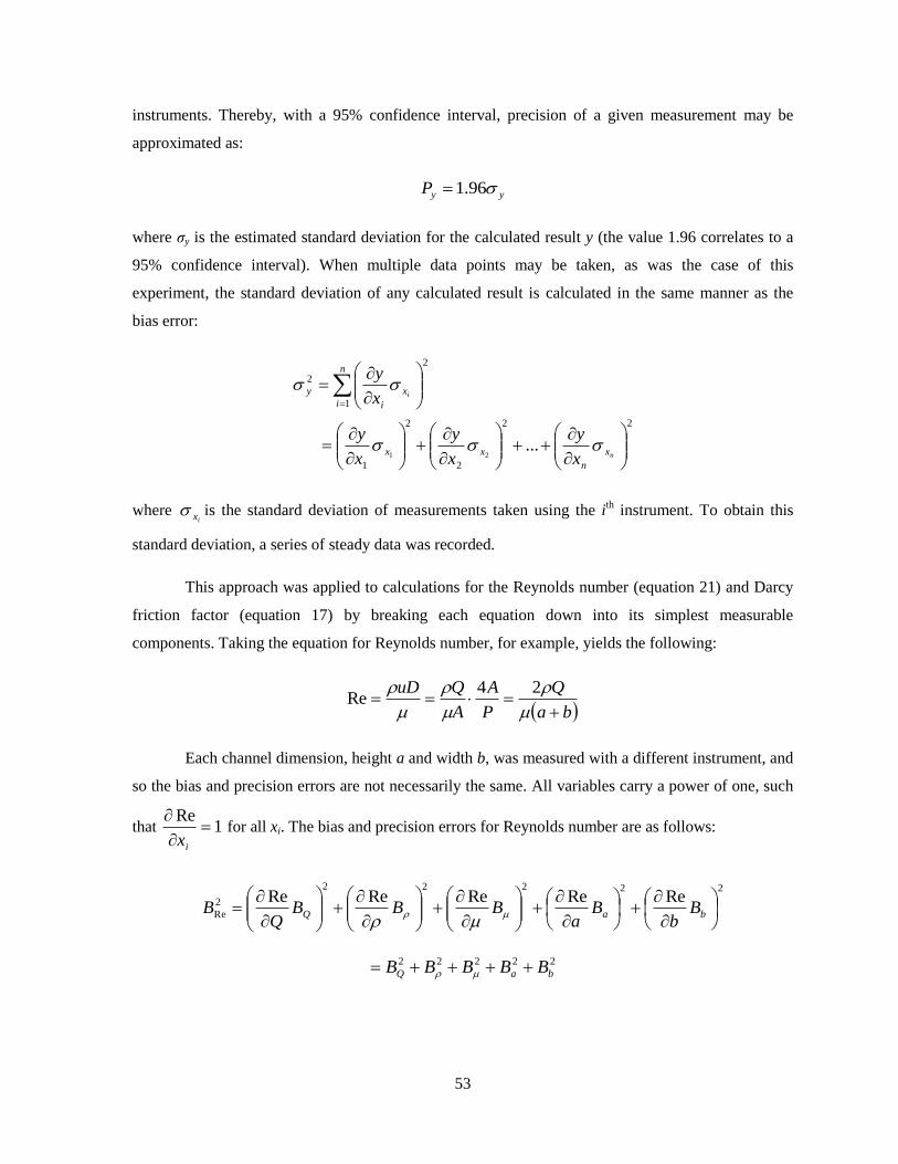
53
instruments. Thereby, with a 95% confidence interval, precision of a given measurement may be
approximated as:
yyP 96.1
where ζy is the estimated standard deviation for the calculated result y (the value 1.96 correlates to a
95% confidence interval). When multiple data points may be taken, as was the case of this
experiment, the standard deviation of any calculated result is calculated in the same manner as the
bias error:
22
2
2
1
2
1
2
...21
n
i
x
n
xx
n
i
x
i
y
x
y
x
y
x
y
x
y
where ix is the standard deviation of measurements taken using the i
th instrument. To obtain this
standard deviation, a series of steady data was recorded.
This approach was applied to calculations for the Reynolds number (equation 21) and Darcy
friction factor (equation 17) by breaking each equation down into its simplest measurable
components. Taking the equation for Reynolds number, for example, yields the following:
ba
Q
P
A
A
QuD
24Re
Each channel dimension, height a and width b, was measured with a different instrument, and
so the bias and precision errors are not necessarily the same. All variables carry a power of one, such
that 1Re
ix for all xi. The bias and precision errors for Reynolds number are as follows:
22222
2
Re
ReReReReRe
baQ B
bB
aBBB
QB
22222
baQ BBBBB
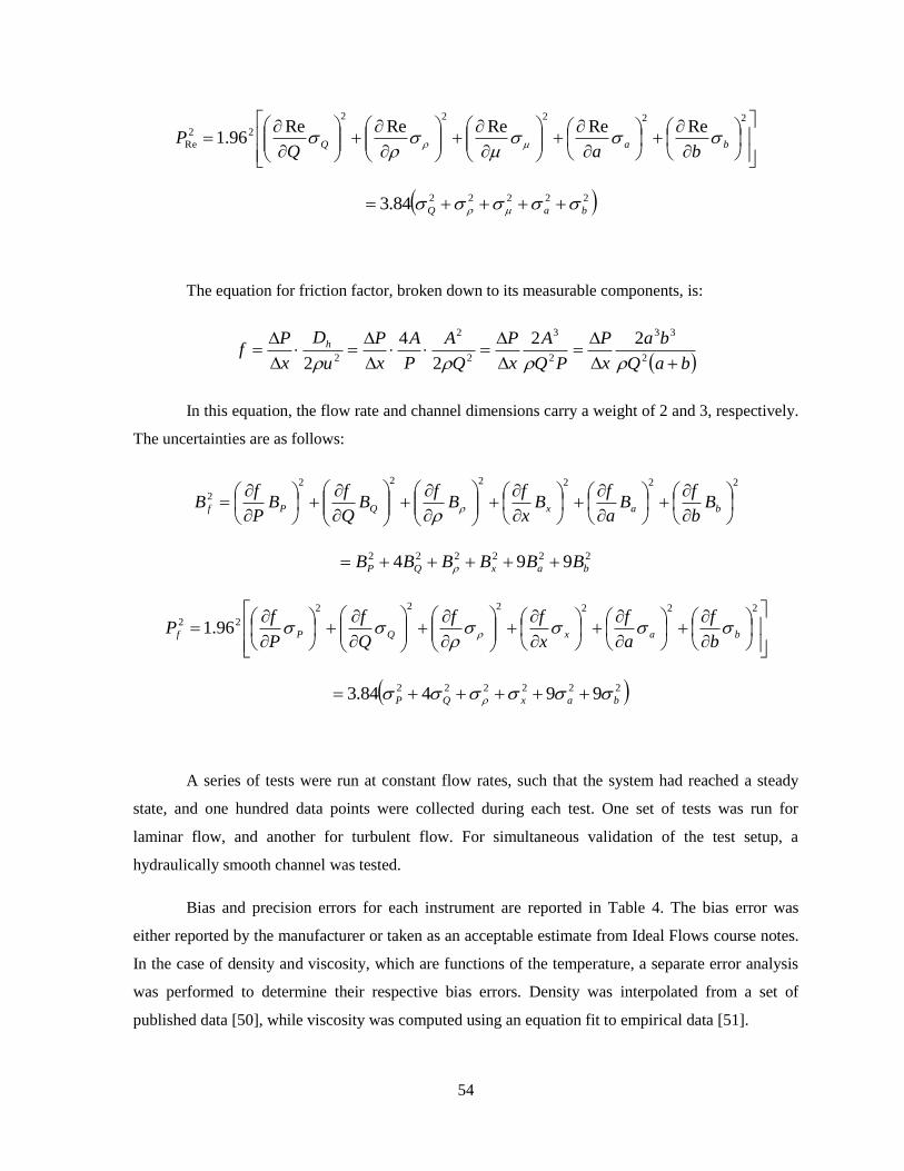
54
22222
22
Re
ReReReReRe96.1 baQ
baQP
2222284.3 baQ
The equation for friction factor, broken down to its measurable components, is:
baQ
ba
x
P
PQ
A
x
P
Q
A
P
A
x
P
u
D
x
Pf h
2
33
2
3
2
2
2
22
2
4
2
In this equation, the flow rate and channel dimensions carry a weight of 2 and 3, respectively.
The uncertainties are as follows:
222222
2
baxQPf B
b
fB
a
fB
x
fB
fB
Q
fB
P
fB
222222 994 baxQP BBBBBB
222222
22 96.1 baxQPfb
f
a
f
x
ff
Q
f
P
fP
222222 99484.3 baxQP
A series of tests were run at constant flow rates, such that the system had reached a steady
state, and one hundred data points were collected during each test. One set of tests was run for
laminar flow, and another for turbulent flow. For simultaneous validation of the test setup, a
hydraulically smooth channel was tested.
Bias and precision errors for each instrument are reported in Table 4. The bias error was
either reported by the manufacturer or taken as an acceptable estimate from Ideal Flows course notes.
In the case of density and viscosity, which are functions of the temperature, a separate error analysis
was performed to determine their respective bias errors. Density was interpolated from a set of
published data [50], while viscosity was computed using an equation fit to empirical data [51].
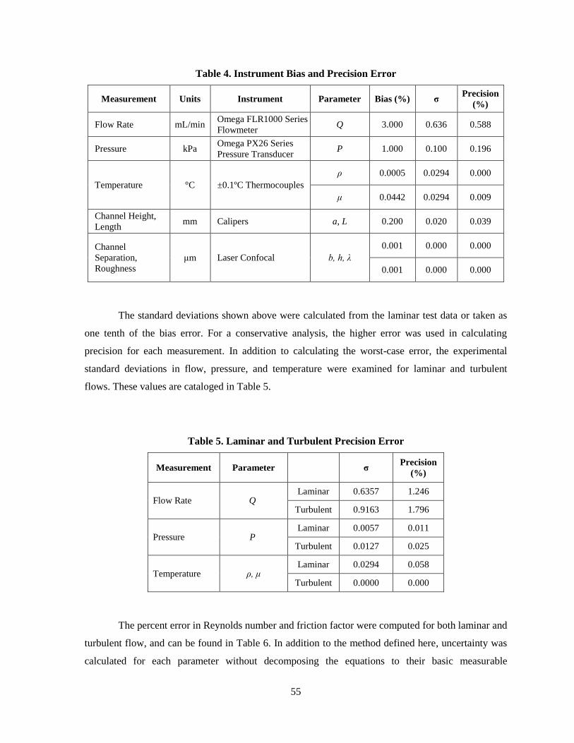
55
Table 4. Instrument Bias and Precision Error
Measurement Units Instrument Parameter Bias (%) σ Precision
(%)
Flow Rate mL/min Omega FLR1000 Series
Flowmeter Q 3.000 0.636 0.588
Pressure kPa Omega PX26 Series
Pressure Transducer P 1.000 0.100 0.196
Temperature °C ±0.1ºC Thermocouples
ρ 0.0005 0.0294 0.000
μ 0.0442 0.0294 0.009
Channel Height,
Length mm Calipers a, L 0.200 0.020 0.039
Channel
Separation,
Roughness
μm Laser Confocal b, h, λ
0.001 0.000 0.000
0.001 0.000 0.000
The standard deviations shown above were calculated from the laminar test data or taken as
one tenth of the bias error. For a conservative analysis, the higher error was used in calculating
precision for each measurement. In addition to calculating the worst-case error, the experimental
standard deviations in flow, pressure, and temperature were examined for laminar and turbulent
flows. These values are cataloged in Table 5.
Table 5. Laminar and Turbulent Precision Error
Measurement Parameter
σ Precision
(%)
Flow Rate Q Laminar 0.6357 1.246
Turbulent 0.9163 1.796
Pressure P Laminar 0.0057 0.011
Turbulent 0.0127 0.025
Temperature ρ, μ Laminar 0.0294 0.058
Turbulent 0.0000 0.000
The percent error in Reynolds number and friction factor were computed for both laminar and
turbulent flow, and can be found in Table 6. In addition to the method defined here, uncertainty was
calculated for each parameter without decomposing the equations to their basic measurable
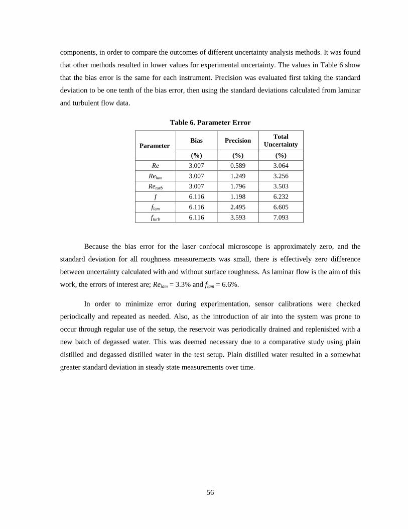
56
components, in order to compare the outcomes of different uncertainty analysis methods. It was found
that other methods resulted in lower values for experimental uncertainty. The values in Table 6 show
that the bias error is the same for each instrument. Precision was evaluated first taking the standard
deviation to be one tenth of the bias error, then using the standard deviations calculated from laminar
and turbulent flow data.
Table 6. Parameter Error
Parameter Bias Precision
Total
Uncertainty
(%) (%) (%)
Re 3.007 0.589 3.064
Relam 3.007 1.249 3.256
Returb 3.007 1.796 3.503
f 6.116 1.198 6.232
flam 6.116 2.495 6.605
fturb 6.116 3.593 7.093
Because the bias error for the laser confocal microscope is approximately zero, and the
standard deviation for all roughness measurements was small, there is effectively zero difference
between uncertainty calculated with and without surface roughness. As laminar flow is the aim of this
work, the errors of interest are; Relam = 3.3% and flam = 6.6%.
In order to minimize error during experimentation, sensor calibrations were checked
periodically and repeated as needed. Also, as the introduction of air into the system was prone to
occur through regular use of the setup, the reservoir was periodically drained and replenished with a
new batch of degassed water. This was deemed necessary due to a comparative study using plain
distilled and degassed distilled water in the test setup. Plain distilled water resulted in a somewhat
greater standard deviation in steady state measurements over time.
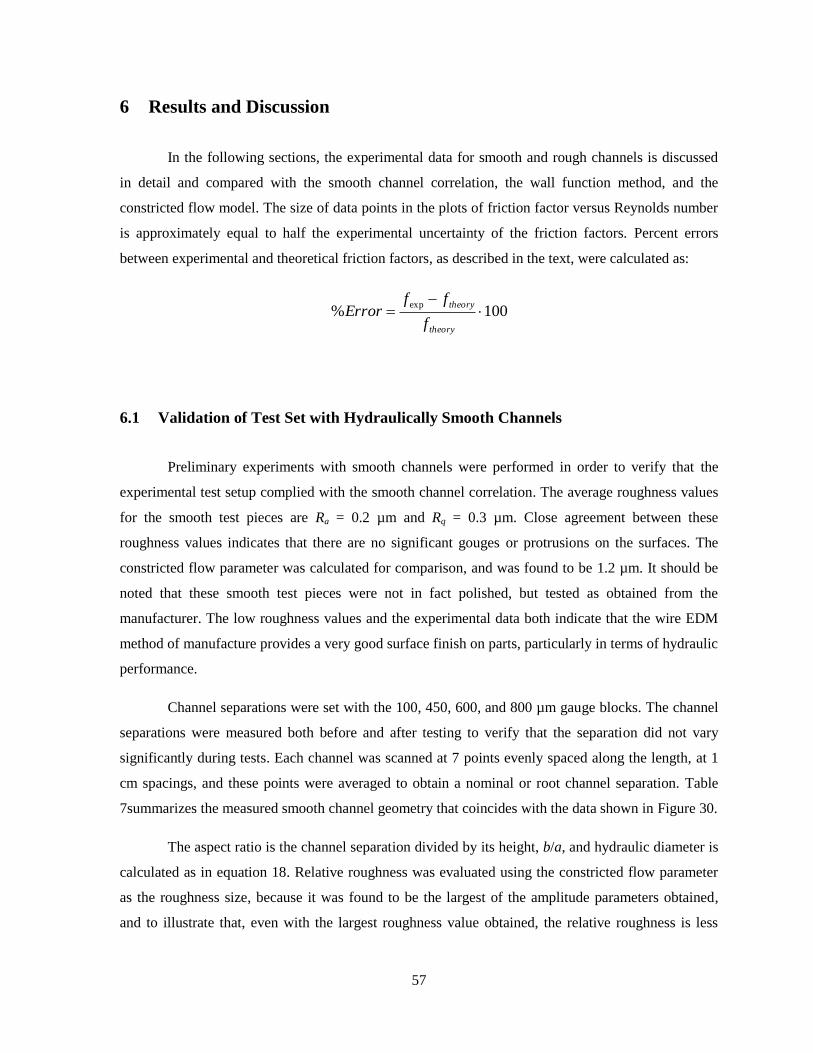
57
6 Results and Discussion
In the following sections, the experimental data for smooth and rough channels is discussed
in detail and compared with the smooth channel correlation, the wall function method, and the
constricted flow model. The size of data points in the plots of friction factor versus Reynolds number
is approximately equal to half the experimental uncertainty of the friction factors. Percent errors
between experimental and theoretical friction factors, as described in the text, were calculated as:
100%exp
theory
theory
f
ffError
6.1 Validation of Test Set with Hydraulically Smooth Channels
Preliminary experiments with smooth channels were performed in order to verify that the
experimental test setup complied with the smooth channel correlation. The average roughness values
for the smooth test pieces are Ra = 0.2 µm and Rq = 0.3 µm. Close agreement between these
roughness values indicates that there are no significant gouges or protrusions on the surfaces. The
constricted flow parameter was calculated for comparison, and was found to be 1.2 µm. It should be
noted that these smooth test pieces were not in fact polished, but tested as obtained from the
manufacturer. The low roughness values and the experimental data both indicate that the wire EDM
method of manufacture provides a very good surface finish on parts, particularly in terms of hydraulic
performance.
Channel separations were set with the 100, 450, 600, and 800 µm gauge blocks. The channel
separations were measured both before and after testing to verify that the separation did not vary
significantly during tests. Each channel was scanned at 7 points evenly spaced along the length, at 1
cm spacings, and these points were averaged to obtain a nominal or root channel separation. Table
7summarizes the measured smooth channel geometry that coincides with the data shown in Figure 30.
The aspect ratio is the channel separation divided by its height, b/a, and hydraulic diameter is
calculated as in equation 18. Relative roughness was evaluated using the constricted flow parameter
as the roughness size, because it was found to be the largest of the amplitude parameters obtained,
and to illustrate that, even with the largest roughness value obtained, the relative roughness is less

58
than 1% for all channel separations. Use of either the average or RMS roughness resulted in relative
roughness values ranging from 0 to 0.2%.
Table 7. Measured Channel Geometry – Smooth Surfaces
Separation Aspect
Ratio
Hydraulic
Diameter
Relative
Roughness
b α Dh e/Dh
μm --- μm ---
101.8 0.01 202 0.6%
377.5 0.03 733 0.2%
548.4 0.04 1051 0.1%
751.0 0.06 1418 0.1%
In fluid flow tests, the flow rate was varied such that the range of Reynolds numbers spanned
from approximately 50 to 4000, although the entire range was not possible for every channel
separation. Reynolds number was calculated using the hydraulic diameter, from the root channel
separations listed in Table 7. Friction factors were calculated using equation 17, and Reynolds
numbers were calculated using equation 21. Theoretical turbulent friction factors were calculated
using the Swamee–Jain equation:
2
9.0Re
74.5
7.3log
25.0
hD
e
f
where e/Dh is the relative roughness and Re is the Reynolds number.
The laminar theory line, shown in black in Figure 30, was calculated using equation 19,
which is intended for use with hydraulically smooth rectangular channels. Due to the small change in
aspect ratio across test cases, there was a difference in friction factor of about 6% when switching
between the smallest and largest channel separations. The laminar theory line shown in Figure 30was
calculated using the largest aspect ratio; α = 0.6.
In all cases, the experimental data was within 10% of conventional laminar theory for smooth
rectangular channels. In the case of the smallest channel separation, 102 µm, the immense pressure
consistently led to leakages above a Reynolds number of 400 across multiple tests. The ability to
observe the behavior of friction factors as the leak occurred in this validation test allowed for early
detection of leaks in rough channel experiments, particularly for the smaller channel separations.

59
Figure 30. Smooth Channel Friction Factor vs. Reynolds Number,
b = 102, 378, 548, and 751 µm
Figure 31 shows a plot of laminar experimental friction factors versus theoretical friction
factors. The purpose of this plot is to illustrate the linearity of the data when compared with theory,
and to show that the data is well within 10% of laminar theory, as the lines in black represent a slope
of 1 and ±10% of that line.
This data indicates that the experimental test set is within the anticipated uncertainty of 6.6%
for the friction factor in the laminar regime. The greatest deviation from the smooth channel
correlation occurred for the smallest channel separation, which is not entirely unexpected, as the
literature indicated friction factors increase as channel size decreases.
Laminar
Turbulent
b = 102 μm
b = 378 μm
b = 548 μm
b = 751 μm
Re
f
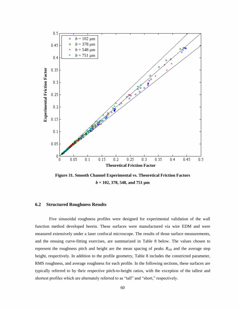
60
Figure 31. Smooth Channel Experimental vs. Theoretical Friction Factors
b = 102, 378, 548, and 751 µm
6.2 Structured Roughness Results
Five sinusoidal roughness profiles were designed for experimental validation of the wall
function method developed herein. These surfaces were manufactured via wire EDM and were
measured extensively under a laser confocal microscope. The results of those surface measurements,
and the ensuing curve-fitting exercises, are summarized in Table 8 below. The values chosen to
represent the roughness pitch and height are the mean spacing of peaks RSM and the average step
height, respectively. In addition to the profile geometry, Table 8 includes the constricted parameter,
RMS roughness, and average roughness for each profile. In the following sections, these surfaces are
typically referred to by their respective pitch-to-height ratios, with the exception of the tallest and
shortest profiles which are alternately referred to as “tall” and “short,” respectively.
b = 102 μm
b = 378 μm
b = 548 μm
b = 751 μm
Theoretical Friction Factor
Exp
erim
enta
l F
rict
ion
Fact
or

61
Table 8. Test Matrix Summary: Roughness Geometry - Measured
Geometry Average Roughness
Pitch Height Aspect
Ratio
Constricted
Parameter RMS
Arithmetic
Mean
λ h λ/h εFp Rq Ra
μm μm --- μm μm μm
249.5 131.0 2 85.5 29.8 25.4
149.8 49.6 3 27.7 9.9 8.6
250.2 49.4 5 28.3 9.7 8.5
400.4 49.6 8 33.8 10.8 9.0
250.6 35.6 7 17.5 5.8 5.0
The five roughness profiles were tested experimentally for four channel separations each,
with the exception of the profile of the lowest peak height, for which only three channel separations
were tested. Channel separation was measured as described for the smooth channel, but the
measurement was taken in the smooth valleys, between roughness peaks, so as to obtain the root
separation required for the theoretical assessment. In a number of cases, there was some discrepancy
between measurements before and after testing, or bowing of the roughness test pieces would occur.
Figure 32 shows a plot of the separation values measured before and after testing the short profile (h
= 31.25 μm, λ = 250 μm) with the 450 µm gauge blocks.
Figure 32. Deviation in Channel Separation Measured Before and After Flow Testing
Using 450 µm Gauge Blocks and λ/h = 7 Surface
The average separation measured before the test represented by Figure 32 was 418.6 µm, and
439.0 µm after. A deviation of about 20 µm is quite significant at this scale, and could have severe
Before
Location
Ch
an
nel
Sep
ara
tion
(μ
m) After

62
effects on much taller roughness profiles. It is also necessary to note that the separation is smallest at
the ends and greatest in the middle in this figure, indicating that the channel was bowed. Therefore,
the clamping was not even along the channel length, and the flow data should be retaken. In all, a
minimum of 5 trials per test case were run in order to assure that the separation and the resulting data
were consistent. Although the precision gauge blocks provide similar channel separations between
test cases, those separations were not exactly as designed due to differences between roughness
profiles. The following table details the measured channel separations for each test condition, as well
as the associated relative roughness values. Channel geometry is identified by the pitch-to-height ratio
in the left-hand column.
Table 9. Test Matrix Summary: Channel Geometry - Measured
Profile Channel Dimensions
Pitch-to-
Height
Ratio
Separation Aspect
Ratio
Hydraulic
Diameter
Relative
Roughness
Relative
Roughness
Height-
Separation
Ratio
λ/h b α Dh h/Dh εFp/Dh h/b
--- μm --- μm --- --- ---
2
377.0 0.03 732 18% 12% 0.35
536.2 0.04 1029 13% 8% 0.24
754.6 0.06 1425 9% 6% 0.17
936.9 0.07 1745 8% 5% 0.14
3
230.3 0.02 452 11% 6% 0.22
413.7 0.03 801 6% 3% 0.12
551.8 0.04 1058 5% 3% 0.09
751.3 0.06 1419 3% 2% 0.07
5
230.5 0.02 453 11% 6% 0.21
414.1 0.03 802 6% 4% 0.12
577.2 0.05 1104 4% 3% 0.09
780.3 0.06 1470 3% 2% 0.06
8
257.7 0.02 505 10% 7% 0.19
444.0 0.03 858 6% 4% 0.11
593.4 0.05 1134 4% 3% 0.08
791.0 0.06 1489 3% 2% 0.06
7
231.4 0.02 455 8% 4% 0.15
439.0 0.03 849 4% 2% 0.08
571.8 0.05 1094 3% 2% 0.06
To summarize, the overall range of channel separations tested was 230.3 to 936.9 µm, which
corresponds to a range of hydraulic diameters of 452 to 1745 µm. Relative roughness ranged from 2%
to 12%, using the constricted parameter. The roughness height to channel separation ratio h/b ranged
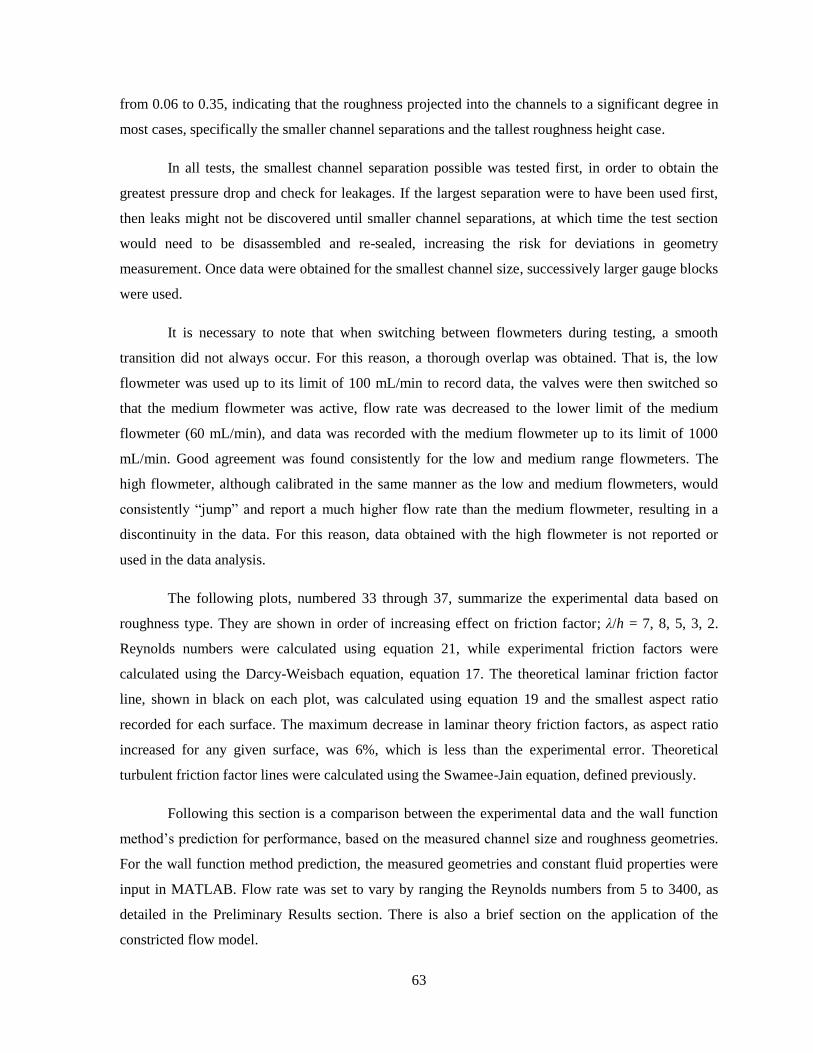
63
from 0.06 to 0.35, indicating that the roughness projected into the channels to a significant degree in
most cases, specifically the smaller channel separations and the tallest roughness height case.
In all tests, the smallest channel separation possible was tested first, in order to obtain the
greatest pressure drop and check for leakages. If the largest separation were to have been used first,
then leaks might not be discovered until smaller channel separations, at which time the test section
would need to be disassembled and re-sealed, increasing the risk for deviations in geometry
measurement. Once data were obtained for the smallest channel size, successively larger gauge blocks
were used.
It is necessary to note that when switching between flowmeters during testing, a smooth
transition did not always occur. For this reason, a thorough overlap was obtained. That is, the low
flowmeter was used up to its limit of 100 mL/min to record data, the valves were then switched so
that the medium flowmeter was active, flow rate was decreased to the lower limit of the medium
flowmeter (60 mL/min), and data was recorded with the medium flowmeter up to its limit of 1000
mL/min. Good agreement was found consistently for the low and medium range flowmeters. The
high flowmeter, although calibrated in the same manner as the low and medium flowmeters, would
consistently “jump” and report a much higher flow rate than the medium flowmeter, resulting in a
discontinuity in the data. For this reason, data obtained with the high flowmeter is not reported or
used in the data analysis.
The following plots, numbered 33 through 37, summarize the experimental data based on
roughness type. They are shown in order of increasing effect on friction factor; λ/h = 7, 8, 5, 3, 2.
Reynolds numbers were calculated using equation 21, while experimental friction factors were
calculated using the Darcy-Weisbach equation, equation 17. The theoretical laminar friction factor
line, shown in black on each plot, was calculated using equation 19 and the smallest aspect ratio
recorded for each surface. The maximum decrease in laminar theory friction factors, as aspect ratio
increased for any given surface, was 6%, which is less than the experimental error. Theoretical
turbulent friction factor lines were calculated using the Swamee-Jain equation, defined previously.
Following this section is a comparison between the experimental data and the wall function
method‟s prediction for performance, based on the measured channel size and roughness geometries.
For the wall function method prediction, the measured geometries and constant fluid properties were
input in MATLAB. Flow rate was set to vary by ranging the Reynolds numbers from 5 to 3400, as
detailed in the Preliminary Results section. There is also a brief section on the application of the
constricted flow model.
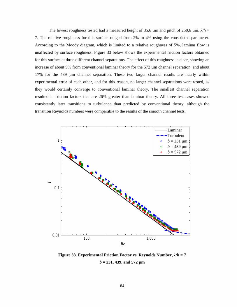
64
The lowest roughness tested had a measured height of 35.6 µm and pitch of 250.6 µm, λ/h =
7. The relative roughness for this surface ranged from 2% to 4% using the constricted parameter.
According to the Moody diagram, which is limited to a relative roughness of 5%, laminar flow is
unaffected by surface roughness. Figure 33 below shows the experimental friction factors obtained
for this surface at three different channel separations. The effect of this roughness is clear, showing an
increase of about 9% from conventional laminar theory for the 572 µm channel separation, and about
17% for the 439 µm channel separation. These two larger channel results are nearly within
experimental error of each other, and for this reason, no larger channel separations were tested, as
they would certainly converge to conventional laminar theory. The smallest channel separation
resulted in friction factors that are 26% greater than laminar theory. All three test cases showed
consistently later transitions to turbulence than predicted by conventional theory, although the
transition Reynolds numbers were comparable to the results of the smooth channel tests.
Figure 33. Experimental Friction Factor vs. Reynolds Number, λ/h = 7
b = 231, 439, and 572 µm
Laminar
Turbulent
b = 231 μm
b = 439 μm
b = 572 μm
Re
f
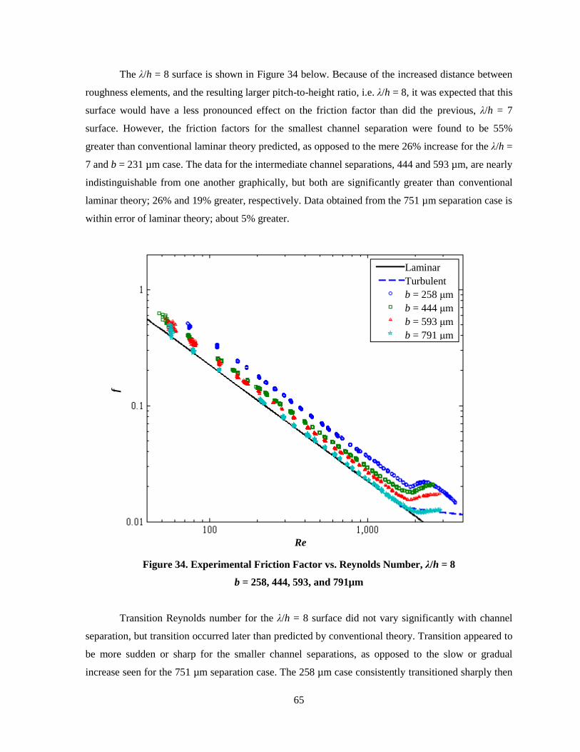
65
The λ/h = 8 surface is shown in Figure 34 below. Because of the increased distance between
roughness elements, and the resulting larger pitch-to-height ratio, i.e. λ/h = 8, it was expected that this
surface would have a less pronounced effect on the friction factor than did the previous, λ/h = 7
surface. However, the friction factors for the smallest channel separation were found to be 55%
greater than conventional laminar theory predicted, as opposed to the mere 26% increase for the λ/h =
7 and b = 231 µm case. The data for the intermediate channel separations, 444 and 593 µm, are nearly
indistinguishable from one another graphically, but both are significantly greater than conventional
laminar theory; 26% and 19% greater, respectively. Data obtained from the 751 µm separation case is
within error of laminar theory; about 5% greater.
Figure 34. Experimental Friction Factor vs. Reynolds Number, λ/h = 8
b = 258, 444, 593, and 791µm
Transition Reynolds number for the λ/h = 8 surface did not vary significantly with channel
separation, but transition occurred later than predicted by conventional theory. Transition appeared to
be more sudden or sharp for the smaller channel separations, as opposed to the slow or gradual
increase seen for the 751 µm separation case. The 258 µm case consistently transitioned sharply then
Laminar
Turbulent
b = 258 μm
b = 444 μm
b = 593 μm
b = 791 μm
Re
f

66
gradually decreased in all trials. Similar behavior of decreasing experimental friction factors was
observed for the smooth channel when the 150 µm gauge block was used, and leakage ensued. This
may indicate that for this test case, had flow rate been increased further, the test section may have
proceeded to exhibit a slow leak at the inlet or outlet headers, as these were the areas prone to leak in
high pressure flows.
Figure 35. Experimental Friction Factor vs. Reynolds Number, λ/h = 5
b = 231, 414, 577, and 780 µm
A pitch-to-height ratio of 5, as is the case in Figure 35 above, is indicative of transitional
roughness (between k- and d-types). This roughness height is the same as in the λ/h = 8 plot (Figure
34), but the pitch is significantly smaller; 250.2 μm. For this surface, the largest channel separation
tested, 780 µm, resulted in friction factors that were 23% greater than the laminar theory predicted.
The next smaller channel separations, 577 and 414 µm, resulted in laminar friction factors 36% and
59% greater than conventional theory, respectively. The smallest channel separation, 231 µm,
resulted in laminar friction factors that were 142% above conventional laminar theory. The transition
Laminar
Turbulent
b = 231 μm
b = 414 μm
b = 577 μm
b = 780 μm
Re
f

67
Reynolds number remained about the same for each channel separation, but as channel separation
decreased, the transition became more abrupt, similar to the behavior of the λ/h = 8 surface.
Figure 36, below, shows the results for the λ/h = 3 surface, where the height remained the
same as with the previous two plots, approximately 50 µm, but the pitch was the smallest attainable
by wire EDM, about 150 µm. Similar to every set of experiments shown thus far, as the channel
separation decreased, the friction factor increased. The interesting thing to note with this surface is
that there is little difference between this and the previous λ/h = 5 case, where the pitch was 250.2
µm. The largest channel separation for these surfaces, 751 µm, resulted in lower friction factors than
the previous case, at 16% greater than laminar theory. The 552 and 414 µm channel separations saw a
negligible increase compared to the λ/h = 5 surfaces, whereas the 230 µm separation yielded slightly
lower friction factors, at 125% above laminar theory. For this roughness pitch, transition occurred
later for every channel separation than in the previous λ/h = 5 case, but the same pattern of
increasingly abrupt transition for decreasing channel size is still shown.
Figure 36. Experimental Friction Factor vs. Reynolds Number, λ/h = 3
b = 230, 414, 552, and 751 µm
Laminar
Turbulent
b = 230 μm
b = 414 μm
b = 552 μm
b = 751 μm
Re
f

68
The first thing to note for Figure 37 below is that, due to the increased roughness height of
131 µm, the 250 µm gauge blocks used for each previous surface could not be used. Thus the smallest
channel separation is 377 µm. Also, because the 800 µm gauge blocks (resultant separation of 755
µm) had not resulted in friction factors comparable to smooth channel theory, the largest gauge block
(1000 µm, resultant separation of 937 µm) was used. As channel size decreased, friction factor
increased, and so the trend is consistent across all data sets. However, this roughness profile, and not
the λ/h = 8 profile, as noted by Coleman et al. [37] shows the most pronounced effect on friction
factor, well into the minichannel range. Experimental friction factors for the largest channel
separation were 71% greater than predicted by laminar theory, and for the smallest channel separation
were 266% greater. Transition to turbulence for this surface occurred at increasingly lower Reynolds
numbers as channel separation decreased, as can be seen in Figure 37. This differs from every
previous test case, which saw greater transitional Reynolds numbers.
Figure 37. Experimental Friction Factor vs. Reynolds Number, λ/h = 2
b = 377, 536, 755, and 937 µm
Laminar
Turbulent
b = 377 μm
b = 536 μm
b = 755 μm
b = 937 μm
Re
f
69
Although turbulent flow was not one of the objectives of this work, all experiments were run
at least up to the transition Reynolds number, which allowed for some observations to be made
regarding the effect of roughness on transition. Transitional behavior has been discussed for each test
case thus far, in terms of the shape or suddenness of the departure from laminar flow, as well as the
relative critical Reynolds numbers. In general, transition occurred around Re = 1800, though some
test cases saw an earlier transition as channel size decreased, particularly for the taller roughness
cases, or the lower λ/h surfaces. The λ/h = 2 surface, for example, began to transition as early as Re =
370 for the smallest channel separation b = 377 μm, and Re = 780 for b = 536 μm.
As channel measurements were recorded throughout the course of testing, theoretical friction
factors were calculated using the wall function method and the constricted flow method. These
theoretical values were kept separate initially so as to let the data speak for itself. In the following
sections, the experimental data is compared with the friction factors predicted by the wall function
method and the constricted flow model. In addition, the data is compared more thoroughly and
discussed more in-depth, in an attempt to ascertain the effects of changing pitch, height, and channel
separation on flow.
6.3 Comparison with Wall Function Method
The next five figures show the previous experimental data plotted with the results of the wall
function method. The theoretical friction factors were calculated using the MATLAB code shown in
Appendix A. Measured channel geometry and roughness geometry were the only parameters input
into the code. Fluid properties were assumed constant, and a range of flow rates were chosen such
that the Reynolds numbers ranged from 5 to 3400. The same laminar and turbulent theory lines shown
in previous plots (in black and blue, respectively) were maintained in these for comparison purposes.
In the plot legends, the experimental data is referred to by the channel separation followed by “exp”
and wall function method results are the channel separation followed by “theory.”
The wall function method does not attempt to predict a critical Reynolds number, and so no
discussion of transition will be found in this section. Extension of the current theory to turbulent flow
is an item for future work.
It was shown previously that the surface with the lowest roughness height h = 35.6 µm,
resulting in a pitch-to-height ratio λ/h = 7, had the least effect on friction factors for laminar flow as
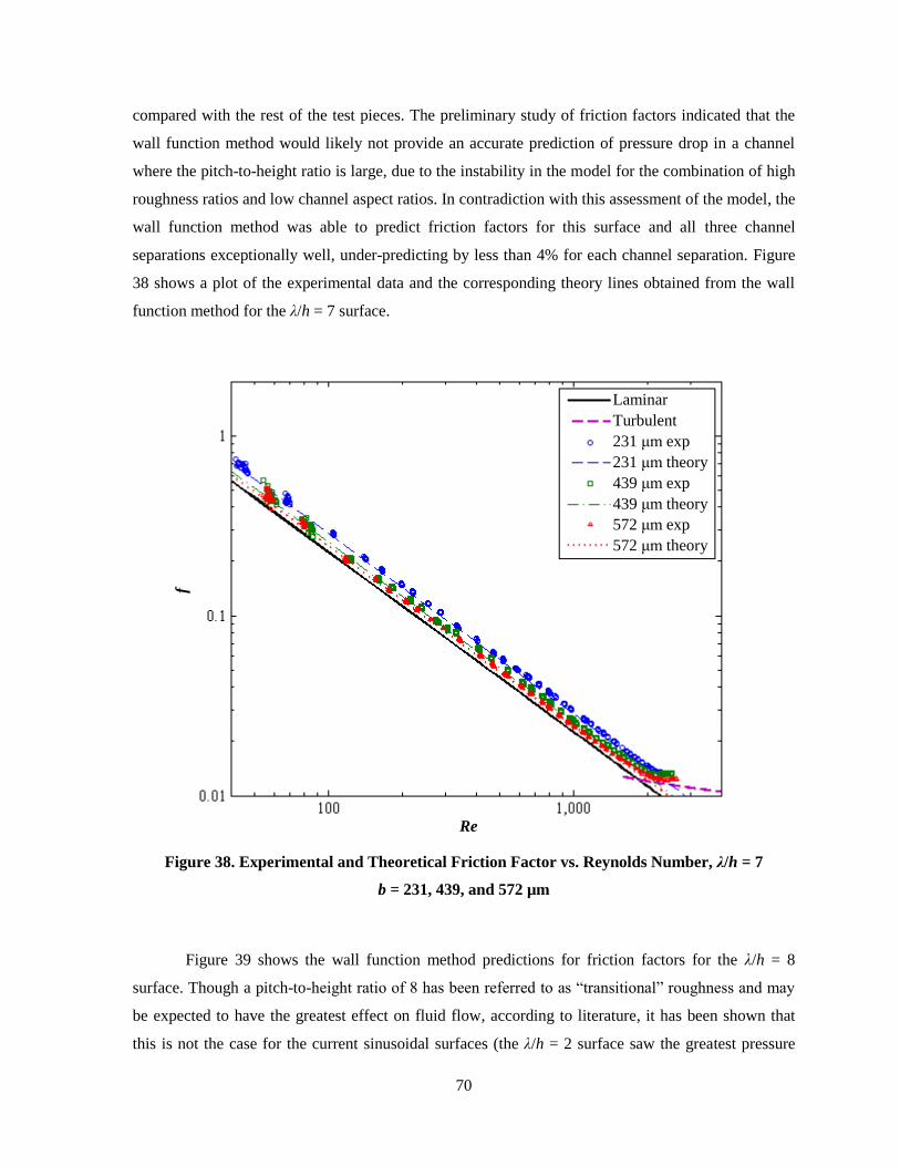
70
compared with the rest of the test pieces. The preliminary study of friction factors indicated that the
wall function method would likely not provide an accurate prediction of pressure drop in a channel
where the pitch-to-height ratio is large, due to the instability in the model for the combination of high
roughness ratios and low channel aspect ratios. In contradiction with this assessment of the model, the
wall function method was able to predict friction factors for this surface and all three channel
separations exceptionally well, under-predicting by less than 4% for each channel separation. Figure
38 shows a plot of the experimental data and the corresponding theory lines obtained from the wall
function method for the λ/h = 7 surface.
Figure 38. Experimental and Theoretical Friction Factor vs. Reynolds Number, λ/h = 7
b = 231, 439, and 572 µm
Figure 39 shows the wall function method predictions for friction factors for the λ/h = 8
surface. Though a pitch-to-height ratio of 8 has been referred to as “transitional” roughness and may
be expected to have the greatest effect on fluid flow, according to literature, it has been shown that
this is not the case for the current sinusoidal surfaces (the λ/h = 2 surface saw the greatest pressure
Laminar
Turbulent
231 μm exp
231 μm theory
439 μm exp
439 μm theory
572 μm exp
572 μm theory
Re
f
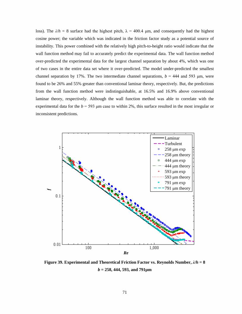
71
loss). The λ/h = 8 surface had the highest pitch, λ = 400.4 μm, and consequently had the highest
cosine power; the variable which was indicated in the friction factor study as a potential source of
instability. This power combined with the relatively high pitch-to-height ratio would indicate that the
wall function method may fail to accurately predict the experimental data. The wall function method
over-predicted the experimental data for the largest channel separation by about 4%, which was one
of two cases in the entire data set where it over-predicted. The model under-predicted the smallest
channel separation by 17%. The two intermediate channel separations, b = 444 and 593 μm, were
found to be 26% and 55% greater than conventional laminar theory, respectively. But, the predictions
from the wall function method were indistinguishable, at 16.5% and 16.9% above conventional
laminar theory, respectively. Although the wall function method was able to correlate with the
experimental data for the b = 593 μm case to within 2%, this surface resulted in the most irregular or
inconsistent predictions.
Figure 39. Experimental and Theoretical Friction Factor vs. Reynolds Number, λ/h = 8
b = 258, 444, 593, and 791µm
Laminar
Turbulent
258 μm exp
258 μm theory
444 μm exp
444 μm theory
593 μm exp
593 μm theory
791 μm exp
791 μm theory
Re
f

72
The following figure shows the experimental data and wall function predictions for the λ/h =
5 surface. The wall function method significantly under-predicted friction factors for all channel
separations for this surface (see Figure 40). The data for the two largest channel separations, b = 577
and 780 μm, fall 13% and 18% above predictions from the wall function method, respectively. Data
for b = 414 μm exceeded the constricted flow method‟s prediction by 29%, and the b = 231 μm
exceeded it by 88%. It is an interesting observation that the wall function method for b = 231 μm
correlates exceptionally well (to within 4%) with the experimental data for b = 414 μm, and the same
is true for the next two larger channel separations. Though the wall function method was thought to
be capable of predicting friction factors for higher values of λ/h, this roughness profile does not
adhere to the wall function method‟s predictions any more than the previous roughness profile.
Figure 40. Experimental and Theoretical Friction Factor vs. Reynolds Number, λ/h = 5
b = 231, 414, 577, and 780 µm
The λ/h = 3 surface has same roughness height and slope as the λ/h = 5 surface, but the
roughness elements are more closely spaced. The similarities in experimental data for these two
surfaces were discussed in the previous section. Figure 41 below shows the wall function method‟s
Laminar
Turbulent
231 μm exp
231 μm theory
414 μm exp
414 μm theory
577 μm exp
577 μm theory
780 μm exp
780 μm theory
Re
f

73
predictions for the λ/h = 3 surface below. For the largest channel separation, the wall function
predicted experimental friction factors exactly, with 0% error. The next channel separation‟s data fell
within 3% of the wall function method‟s prediction. For b = 414 and 230 μm, however, the data fell
27% and 23% above the wall function method‟s prediction, respectively.
Figure 41. Experimental and Theoretical Friction Factor vs. Reynolds Number, λ/h = 3
b = 230, 414, 552, and 751 µm
Figure 42 shows the wall function method‟s predictions for the highest roughness tested; the
λ/h = 2 surface. Excellent agreement was found for the smallest channel separations, with
experimental data falling within 2% of the wall function method friction factors for both b= 536 and
377 μm. This agreement was foreshadowed in the preliminary results section, where the range of low
pitch-to-height ratios and small channel aspect ratios were expected to result in the greatest friction
factors with the least instability. Percent error was somewhat different for the two larger channel
separations; friction factors for b = 755 μm were 25% greater than the wall function method, whereas
for b = 937 μm they were 8% lower. This is the second test case where the wall function method
over-predicted frictional losses.
Laminar
Turbulent
230 μm exp
230 μm theory
414 μm exp
414 μm theory
552 μm exp
552 μm theory
751 μm exp
751 μm theory
Re
f

74
Figure 42. Experimental and Theoretical Friction Factor vs. Reynolds Number, λ/h = 2
b = 377, 536, 755, and 937 µm
Of the nineteen test cases presented here, nine were predicted to within experimental error by
the wall function method. Those cases include the two largest λ/h surfaces, with better agreement seen
for the larger channel separations, and the two smallest λ/h surfaces, with better agreement for the
larger separations and the λ/h = 3 surface, and better agreement for the smaller separations and the λ/h
= 2 surface. The λ/h = 5 surface exhibited the poorest agreement with the wall function method‟s
predictions for all channel separations tested.
A summary of percent error between the experimental data and both the smooth channel
correlation and the wall function method for each test case is provided in Table 10 below. All
experimental friction factors were found to be greater than conventional theory and percent difference
increased as channel separation decreased, with the difference becoming more pronounced as λ/h
decreased. Similarly, experimental friction factors were found to be greater than the wall function
method‟s predictions in all cases but for the largest channel separations for λ/h = 8 and 2. The cases
for which percent error is less than experimental error are highlighted in grey in Table 10.
Laminar
Turbulent
377 μm exp
377 μm theory
536 μm exp
536 μm theory
755 μm exp
755 μm theory
937 μm exp
937 μm theory
Re
f
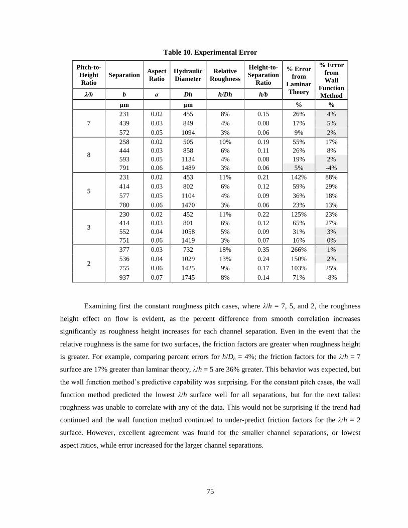
75
Table 10. Experimental Error
Pitch-to-
Height
Ratio
Separation Aspect
Ratio
Hydraulic
Diameter
Relative
Roughness
Height-to-
Separation
Ratio
% Error
from
Laminar
Theory
% Error
from
Wall
Function
Method λ/h b α Dh h/Dh h/b
μm μm % %
7
231 0.02 455 8% 0.15 26% 4%
439 0.03 849 4% 0.08 17% 5%
572 0.05 1094 3% 0.06 9% 2%
8
258 0.02 505 10% 0.19 55% 17%
444 0.03 858 6% 0.11 26% 8%
593 0.05 1134 4% 0.08 19% 2%
791 0.06 1489 3% 0.06 5% -4%
5
231 0.02 453 11% 0.21 142% 88%
414 0.03 802 6% 0.12 59% 29%
577 0.05 1104 4% 0.09 36% 18%
780 0.06 1470 3% 0.06 23% 13%
3
230 0.02 452 11% 0.22 125% 23%
414 0.03 801 6% 0.12 65% 27%
552 0.04 1058 5% 0.09 31% 3%
751 0.06 1419 3% 0.07 16% 0%
2
377 0.03 732 18% 0.35 266% 1%
536 0.04 1029 13% 0.24 150% 2%
755 0.06 1425 9% 0.17 103% 25%
937 0.07 1745 8% 0.14 71% -8%
Examining first the constant roughness pitch cases, where λ/h = 7, 5, and 2, the roughness
height effect on flow is evident, as the percent difference from smooth correlation increases
significantly as roughness height increases for each channel separation. Even in the event that the
relative roughness is the same for two surfaces, the friction factors are greater when roughness height
is greater. For example, comparing percent errors for h/Dh = 4%; the friction factors for the λ/h = 7
surface are 17% greater than laminar theory, λ/h = 5 are 36% greater. This behavior was expected, but
the wall function method‟s predictive capability was surprising. For the constant pitch cases, the wall
function method predicted the lowest λ/h surface well for all separations, but for the next tallest
roughness was unable to correlate with any of the data. This would not be surprising if the trend had
continued and the wall function method continued to under-predict friction factors for the λ/h = 2
surface. However, excellent agreement was found for the smaller channel separations, or lowest
aspect ratios, while error increased for the larger channel separations.

76
The three cases for constant roughness height, λ/h = 8, 5, and 3, all resulted in comparable
relative roughness values for the channel separations tested, reinforcing the statement that the concept
of relative roughness is not applicable for structured roughness elements. It was the λ/h = 5 surface
that exhibited the greatest effect on fluid flow, however, and not the λ/h = 8 surface that was noted in
the literature. On either side of the surface, for the lower and higher roughness pitches, percent error
between the experimental data and laminar theory decreased, with the exception of the λ/h = 3 surface
and 414 μm channel separation. The same trend can be seen in the percent errors between
experimental friction factors and those predicted by the wall function method.
Another method for comparison of experimental data is through the use of the Poiseuille
number, Po = f·Re, which is a constant in the laminar flow regime. This parameter varies with
channel geometry, but was also found to increase with increasing roughness height, as the roughness
caused laminar friction factors to increase, but had minimal effect on the Reynolds number. The
variation in experimental Poiseuille number with roughness type and channel aspect ratio is shown in
Figure 43 below. For the smooth channel case, the Poiseuille number was constant, Po = 23, for all
channel separations.
Figure 43. Experimental Poiseuille Number vs. Channel Aspect Ratio
Smooth
λ/h = 7
λ/h = 8
λ/h = 5
λ/h = 3
λ/h = 2
Aspect Ratio (b/a)
Po
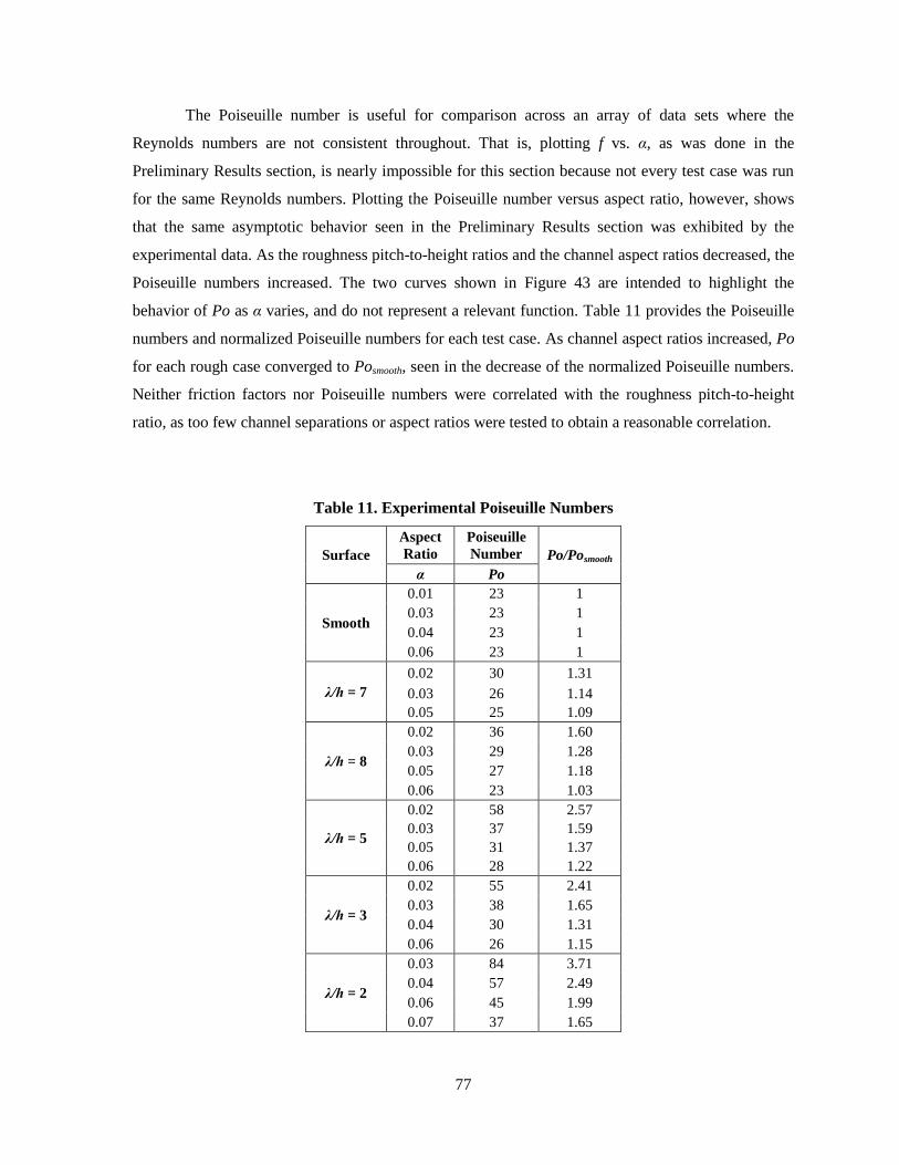
77
The Poiseuille number is useful for comparison across an array of data sets where the
Reynolds numbers are not consistent throughout. That is, plotting f vs. α, as was done in the
Preliminary Results section, is nearly impossible for this section because not every test case was run
for the same Reynolds numbers. Plotting the Poiseuille number versus aspect ratio, however, shows
that the same asymptotic behavior seen in the Preliminary Results section was exhibited by the
experimental data. As the roughness pitch-to-height ratios and the channel aspect ratios decreased, the
Poiseuille numbers increased. The two curves shown in Figure 43 are intended to highlight the
behavior of Po as α varies, and do not represent a relevant function. Table 11 provides the Poiseuille
numbers and normalized Poiseuille numbers for each test case. As channel aspect ratios increased, Po
for each rough case converged to Posmooth, seen in the decrease of the normalized Poiseuille numbers.
Neither friction factors nor Poiseuille numbers were correlated with the roughness pitch-to-height
ratio, as too few channel separations or aspect ratios were tested to obtain a reasonable correlation.
Table 11. Experimental Poiseuille Numbers
Surface
Aspect
Ratio
Poiseuille
Number Po/Posmooth
α Po
Smooth
0.01 23 1
0.03 23 1
0.04 23 1
0.06 23 1
λ/h = 7
0.02 30 1.31
0.03 26 1.14
0.05 25 1.09
λ/h = 8
0.02 36 1.60
0.03 29 1.28
0.05 27 1.18
0.06 23 1.03
λ/h = 5
0.02 58 2.57
0.03 37 1.59
0.05 31 1.37
0.06 28 1.22
λ/h = 3
0.02 55 2.41
0.03 38 1.65
0.04 30 1.31
0.06 26 1.15
λ/h = 2
0.03 84 3.71
0.04 57 2.49
0.06 45 1.99
0.07 37 1.65

78
6.4 Comparison with Constricted Flow Model
To review, the constricted flow model makes use of the amplitude parameter εFp in order to
“constrict” the flow. In essence, it serves to account for the boundary layer in rough channel flows,
and has been applied to experimental data in literature in order to force experimental data to adhere to
conventional laminar theory for smooth channels.
Figure 44. Constricted Experimental Friction Factor vs. Reynolds Number, λ/h = 3
b = 230, 414, 552, and 751 µm
In applying the constricted flow model to the data at hand, the friction factors and Reynolds
numbers, equations 17 and 21, respectively, were recalculated using the constricted geometry. Figure
44 provides an example of the outcome for the λ/h = 3 surface. The data shown were within 10% of
laminar theory, the closest fit of all surfaces tested. The remaining test cases resulted in friction
factors consistently lower than laminar theory when the constricted flow model was applied.
Laminar
Turbulent
b = 230 μm
b = 414 μm
b = 552 μm
b = 751 μm
Re
f
79
7 Conclusions
Laminar flow of an incompressible fluid in rectangular channels, possessing two-dimensional
roughness, was investigated from a theoretical standpoint resulting in a model for pressure versus
flow that allowed for the direct input of surface roughness geometry. This model is referred to as the
wall function method. The primary focus was on long, small aspect ratio, rectangular channels in the
mini- or microscale range. Structured roughness of a sinusoidal type was evaluated in order to control
and vary the pitch and height. These surfaces were described by their roughness pitch-to-height ratios,
λ/h. A test set and a series of roughness test pieces were fabricated for experimental assessment of the
applicability of the wall function method.
Standard amplitude, spatial, and shape parameters were evaluated for the rough surfaces
generated in order to determine a combination of parameters relevant to the sinusoidal-type
roughness. The spatial parameter RSM was found to be in exact agreement with the designed
roughness pitch, while the average step height, a non-standard parameter, was found to be in good
agreement with the designed peak height. A more universal parameter is required for measurement of
the peak height, and a method for designing and predicting the cosine power, which controls the peak
slope, is also needed. Relative roughness, εFp/Dh, was found to be an inconsistent means of
representing structured roughness, as it does not vary sufficiently with roughness pitch or shape.
A series of experiments were run with degassed water flowing through channels possessing a
range of roughness types, summarized in Table 13 in Appendix B. In every test case, friction factors
were found to be greater than conventional laminar theory for smooth rectangular ducts. As channel
aspect ratio decreased, or as the hydraulic diameter decreased, the experimental friction factors
increased, with the increase becoming more pronounced for taller and more closely spaced roughness.
No pattern was observed for the cases of constant roughness height and varying pitch, aside from the
intermediate surface, λ/h = 5, exhibiting the largest friction factors of the three. It was noted in the
literature that there is an intermediate pitch-to-height ratio that would yield the greatest effect on fluid
flow. However, in these experiments, it was the smallest pitch-to-height ratio, λ/h = 2, that exhibited
the largest friction factors.
Comparing experimental data with the friction factors obtained from the wall function
method uncovered some unexpected results. First, the surface for which λ/h was greatest (λ/h = 8) was
expected to show more instability than the rest in the wall function method, but data for this surface
was within experimental error of the wall function method for the two larger channel cases. The next
80
largest pitch-to-height ratio was the short profile, λ/h = 7, which was expected to have the least effect
on fluid flow, and was predicted best by the wall function method out of all the sinusoidal surfaces.
The intermediate surface, for which λ/h = 5, was the most unpredictable of the surfaces tested, and
resulted in the poorest comparison with the wall function method. This pitch-to-height ratio is
considered the transition between d-type and k-type roughness. The surface of λ/h = 3 saw friction
factors comparable to those of the λ/h = 5 surface, though were consistently lower. The wall function
method predicted the largest two channel separations for this surface to well within experimental
uncertainty. The final and tallest surface roughness, λ/h = 2, had the most pronounced effect on fluid
flow, with percent errors in excess of 100% compared with smooth channel theory. The wall function
method predicted the two smallest channel separations for this surface exceptionally well, which is
contrary to the previous cases where larger channel separations were predicted successfully.
Though the wall function method had some success, and is consistent with the smooth
channel correlation, only nine of the nineteen rough cases were able to be predicted with the wall
function method. The limits of the lubrication approximation were tested by increasing the Reynolds
number and the surface roughness, and in spite of exceeding those limits, the analysis still saw some
success. A potential reason for the poor predictive capability may be due to the range of Reynolds
numbers tested. The analysis was made for laminar flow, true, but the experimental flows may not
have been laminar enough. In terms of scale analysis, the Reynolds number multiplied by the aspect
ratio, Re·α, should be approximately 1. Though the aspect ratios were sufficiently small, the lowest
flow rates obtained with the experimental test setup were limited to Re ≥ 40. The analysis should be
more successful for Stokes flow.
Other potential sources of error may be alleviated through improvements to the experimental
test setup. Entrance and exit effects that were neglected in the theoretical analysis may not have been
entirely negligible for smaller channel separations. The non-uniformity of the channel cross-section,
although minimized during testing, might imply that the channel could have deflected for higher flow
rates. Alignment of roughness elements may have contributed to uncertainty in the hydraulic
performance of the various surfaces. Uncertainties and errors in instrumentation, measurement, and
measurement locations in general could also be improved.
Overall, the limits of the wall function method were tested and it was shown that it is possible
to predict frictional losses in a significantly rough microchannel without the complex computations of
the fluid in the near wall region.
81
8 Recommendations
As with all experimental reports, more data is required in order to make a definite conclusion.
A greater range of λ, h, and p combinations, with more precise geometric similitude across all cases,
together with the ability to vary channel height, would shed some light on the grey areas of this work.
In addition, a more extensive sensitivity study on these roughness parameters would complete the
information put forth in the Preliminary Results section; more specifically, the effect of varying
roughness height on wall function friction factors should be expanded. A shape parameter must also
be identified to estimate sinusoid power for the roughness studied in this work.
Roughness shape has been noted in the literature as playing a role in fluid flow, and for this
reason different roughness geometries should be tested for comparison with the wall function method.
A series of roughness test pieces with square geometry have been generated to fit in the existing test
set. Smooth continuous functions need to be developed for the new geometries. Alternatively, the
code presented in the Appendix could be modified to allow the user to input profile data for analysis.
This approach would be ineffective for complex geometries, however, as well as for the extended
analysis where the roughness slope is required. The direction of roughness elements may also play a
role, particularly for thermal applications where longitudinal roughness may enhance heat transfer.
Thus another extension of the current work would be to investigate the same roughness profiles
rotated at 90 degrees, such that the peaks and grooves are parallel to the flow, and at other oblique
angles.
A few simple improvements to the experimental apparatus could extend its capabilities into
the turbulent regime. Also, a smaller pump (perhaps a syringe pump) and a lower range flowmeter
would allow for lower Reynolds number data, which is essential for the theoretical analysis presented
herein. Ideally, a single flowmeter that works well over all ranges of flow rate, from Stokes flow to
the fully turbulent regime, would reduce error in switching between flowmeters, reduce the number of
calibrations to be performed, and reduce the amount of data processing.
The test set as-is could easily be enhanced for use with micro-PIV (particle imaging
velocimetry). The aluminum lid may be replaced by a transparent structural plastic, though sealing
would need to be readdressed. This was kept in mind during the design stages, as it would be of great
interest to understand the growth of vortices between the roughness elements studied here. Micro-PIV
would also allow for visual verification of the flow profile development.

82
From the theoretical standpoint, it is imperative that the further analysis based on the
augmented lubrication approximation be carried out. A method for evaluating the inertial integral
must be established, but an approximation may be sufficient. The inertial integral from equation 16 is:
L
xxfxg
x
xf
x
xg
a
Q
0
32
2
)()(
)()(
5
6
To simplify this integral, the wall function slopesx
xg
)(and
x
xf
)( may be taken to be the
maximum slope of an individual asperity on the periodic surface. In the case of the λ/h = 5 surface,
for example, the maximum slope is 1.35, resulting in a maximum slope difference of 2.70. Taking
another simplification, after the constricted flow method, the integral reduces to
70.25
632
2
cfb
L
a
Q
Comparing this integral with the viscous portion gives an indication of the range of
applicability of this augmented lubrication approximation:
127.0
a
Q
Within this criterion, the inertial term is negligible, and the wall function method is sufficient.
If, for example, the flow rate exceeds this limit for the geometry herein, then the augmented
lubrication approximation may provide some improvement.
83
9 References
[1] Moody, L.F., 1944, “Friction factors for pipe flow,” Transactions of ASME, 66, pp. 671-684.
[2] Von Mises, R., 1914, “Elemente der Technischen Hydromechanik,” Leipzig, B.G. Teubner.
[3] Kandlikar, S. G., Schmidt, D., Carrano, A. L., and Taylor, J. B., 2005, “Characterization of
Surface Roughness Effects on Pressure Drop in Single-Phase Flow in Minichannels and
Microchannels,” Physics of Fluids, 17 (10), pp. 962–968.
[4] Brophy, J., 2005, “The Microchannel Revolution,” Focus on Catalysts, 2005 (2), pp. 1-2.
[5] Schlichting, H., 1949, “Vortragsreihe,” (“Lecture Series „Boundary Layer Theory‟ - Part I:
Laminar Flows”) NACA TM No. 1217.
[6] Darcy, H., 1857, “Recherches Experimentales Relatives au Mouvement de L'Eau dans les
Tuyaux,” (“Experimental Research Relating to the Movement of Water in Pipes”), Mallet-
Bachelier, Paris.
[7] Hopf, L., 1923, “Die Messung der Hydraulischen Rauhigkeit,” (“The measurement of
hydraulic roughness”), Zeitschrift für Angewandte Mathematik und Mechanik, 3, pp. 329-
339.
[8] Fromm, K., 1923, “Strömungswiderstand in Rauhen Rohren,” (“Flow resistance in rough
pipes”), Zeitschrift für Angewandte Mathematik und Mechanik, 3, pp. 339-358.
[9] Nikuradse, J., 1933, “Strömungsgesetze in Rauhen Rohren,” (“Laws of Flow in Rough
Pipes”) NACA TM No. 1292.
[10] Colebrook, C.F., 1939, “Turbulent flow in pipes with particular reference to the transition
region between the smooth and rough pipe laws,” Journal of the Institute of Civil Engineers,
4, pp. 133–156.
[11] Kandlikar, S.G., Garimella, S., Li, D., Colin, S., King, M.R., 2006, Heat Transfer and Fluid
Flow in Minichannels and Microchannels, Elsevier, Oxford.
[12] Shah, R.K., 1972, “Laminar Flow Forced Convection Heat Transfer and Friction in Straight
and Curved Ducts – A Summary of Analytical Solutions,” Stanford University, Palo Alto,
CA.
[13] Shah, R. K., 1975, “Laminar Flow Friction and Forced Convection Heat Transfer in Ducts of
Arbitrary Geometry,” International Journal of Heat and Mass Transfer, 18, pp. 849-862.
[14] Mala G.M., Dongqing L.1, Dale J.D., 1997, “Heat Transfer and Fluid Flow in
Microchannels,” International Journal of Heat and Mass Transfer, 40 (13), pp. 3079-3088.

84
[15] Papautsky, I., Gale, B.K., Mohanty, S., Ameel, T.A., Frazier, A.B., 1999, “Effects of
Rectangular Microchannel Aspect Ratio on Laminar Friction Constant,” Proceedings of SPIE
– The International Society for Optical Engineering, Proceedings of the 1999 Microfluidic
Devices and Systems II, Santa Clara.
[16] Wu, H.Y. and Cheng, P., 2003, “Friction Factors in Smooth Trapezoidal Silicon
Microchannels with Different Aspect Ratios,” International Journal of Heat and Mass
Transfer, 46, pp. 2519–2525
[17] Li, Z.X., Du, D.X., Guo, Z.Y., 2003, “Experimental Study on Flow Characteristics of Liquid
in Circular Microtubes,” Microscale Thermophysical Engineering, 7 (3), pp. 253-265.
[18] Pfahler, J., Harley, J., Bau, H., and Zemel, J.N., 1991, “Gas and Liquid Flow in Small
Channels,” Micromechanical Sensors, Actuators, and Systems, ASME, 32, pp. 49-61.
[19] Yu, D., Warrington, R., Barron, R., Ameel, T., 1995, “Experimental and Theoretical
Investigation of Fluid Flow and Heat Transfer in Microtubes,” Proceedings of the 1995
ASME/JSME Thermal Engineering Joint Conference, Maui, Hawaii.
[20] Judy, J., Maynes, Webb, D.B. W., 2002, “Characterization of Frictional Pressure Drop for
Liquid Flows through Microchannels,” International Journal of Heat and Mass Transfer, 45
(17), pp. 3477-3489.
[21] Tu, X. and Hrnjak, P., 2003, “Experimental Investigation of Single-Phase Flow Pressure
Drop Through Rectangular Microchannels,” Proceedings of the 1st International Conference
on Microchannels and Minichannels. Rochester, NY.
[22] A. Bucci, G.P. Celata, M. Cumo, E. Serra, and G. Zummo, 2003, "Water Single-Phase Fluid
Flow and Heat Transfer in Capillary Tubes," Proceedings of the 1st International Conference
on Microchannels and Minichannels. Rochester, NY.
[23] Bavière, R., Ayela, F., Le Person, S. and Favre-Marinet, M., 2005, “Experimental
Characterization of Water Flow through Smooth Rectangular Microchannels,” Physics of
Fluids, 17, 1–4.
[24] Akbari, M., Bahrami, M., and Sinton, D., 2009, “Flow in Rectangular Microchannels: an
Experimental Investigation,” ASME Journal Fluid Engineering, Vol. 131, pp. 041203-1-10.
[25] Peng, X.F., and Peterson, G.P., 1995, “Convective Heat Transfer and Flow Friction for Water
Flow in Microchannel Structures,” International Journal of Heat and Mass Transfer, 39 (12),
pp. 2599-2608.

85
[26] Peng, X.F., Peterson, G.P., and Wang, B.X., 1994, “Frictional Flow Characteristics of Water
Flowing Through Rectangular Microchannels,” Experimental Heat Transfer, 7, pp. 249-264.
[27] Kandlikar, S.G. and Grande, W.J., 2003, “Evolution of Microchannel Flow Passages--
Thermohydraulic Performance and Fabrication Technology,” Heat Transfer Engineering, 24
(1), pp. 3-17.
[28] Mehendale, S.S., Jacobi, A.M., Shah, R.K., 1999, Heat exchangers at micro- and meso-
scales, in: R.K. Shah (Ed.), Compact Heat Exchangers and Enhancement Technology for the
Process Industries, Begell House, New York, pp. 55–74.
[29] Bahrami, M., Yovanovich, M.M., Culham, J.R., 2007, “A Novel Solution for Pressure Drop
in Singly Connected Microchannels,” International Journal of Heat and Mass Transfer, 50,
pp. 2492-2502.
[30] Menezes, P.L., Kishore, and Kailas, S.V., 2008, “Influence of Roughness Parameters on
Coefficient of Friction Under Lubricated Conditions,” Sādhanā, Academy Proceedings in
Engineering Sciences, 33 (3), pp. 181-190.
[31] Schlichting, H., 1936, “Experimentelle Untersuchungen zum Rauhigkeitsproblem,”
(“Experimental Investigation of the Problem of Surface Roughness”) NACA TM No. 823.
[32] Sams, E. W., 1952, “Experimental Investigation of Average Heat Transfer and Friction
Coefficients for Air Flowing in Circular Tubes Having Square-Thread-Type Roughness,”
NACA RM E52D17.
[33] Rawool, A.S., Mitra, S.K., Kandlikar, S.G., 2006, “Numerical Simulation of Flow Through
Microchannels with Designed Roughness,” Microfluidics and Nanofluidics, 2 (3), pp.215-
221.
[34] Wang, X.Q., Yap, C., and Mujumdar, A.S., 2005, “Effects of Two-dimensional Roughness in
Flow in Microchannels,” Journal of Electronic Packaging, 127 (3), pp. 357–361.
[35] Sun, H. and Faghri, M., 2003, “Effect of Surface Roughness on Nitrogen Flow in a
Microchannel Using the Direct Simulation Monte Carlo method,” Numerical Heat Transfer,
Part A: Applications: An International Journal of Computation and Methodology, 43 (1), pp.
1-8.
[36] Jiménez, J., 2004, “Turbulent Flows Over Rough Walls,” Annual Review of Fluid
Mechanics, 36, pp. 173-196.
[37] Coleman, S.E., Nikora, V.I., McLean, S.R., and Schlicke, E., 2007, “Spatially Averaged
Turbulent Flow Over Square Ribs,” Journal of Engineering Mechanics, 133 (2), pp. 194-204.

86
[38] Mala, G.M. and Li, D., 1999, “Flow Characteristics of Water in Microtubes,” International
Journal of Heat and Fluid Flow, 20, pp. 142-148.
[39] Sabry, M.N., 2000, “Scale Effects on Fluid Flow and Heat Transfer in Microchannels,” IEEE
Transactions on Components and Packaging Technologies, 23 (3), pp. 562-567.
[40] Koo, J. and Kleinstreuer, C., 2003 “Liquid Flow in Microchannels: Experimental
Observations and Computational Analyses of Microfluidics Effects,” Journal of
Micromechanics and Microengineering, 13, pp. 568–579.
[41] Kleinstreuer, C. and Koo, J., 2004, “Computational Analysis of Wall Roughness Effects for
Liquid Flow in Micro-conduits,” Journal of Fluids Engineering, 126 (1), pp. 1–9.
[42] Gamrat, G., Favre-Marinet, M., Le Person, S., Bavière, R., and Ayela, F., 2008, “An
Experimental Study and Modelling of Roughness Effects on Laminar Flow in
Microchannels,” Journal of Fluids Mechanics, 594, pp. 399–423.
[43] Gamrat, G., Favre-Marinet, M., and Le Person, S., 2009, Modelling of Roughness Effects on
Heat Transfer in Thermally Fully-developed Laminar Flows through Microchannels,”
International Journal of Thermal Sciences, 48 (12), pp.2203-2214 .
[44] Brackbill, T. P., 2008, “Experimental Investigation on The Effects of Surface Roughness on
Microscale Liquid Flow,” Rochester Institute of Technology, Rochester, NY.
[45] Weinstein, S., 2009, Personal Communication.
[46] Brackbill, T. P. and Kandlikar, S. G., 2006, “Effect of Triangular Roughness Elements on
Pressure Drop and Laminar-Turbulent Transition in Microchannels and Minichannels,”
Proceedings of the 4th International Conference on Nanochannels, Microchannels, and
Minichannels, Limerick, Ireland.
[47] Brackbill, T. P., and Kandlikar, S. G., 2008, “Effects of Roughness on Turbulent Flow in
Microchannels and Minichannels,” Proceedings of the Sixth International ASME Conference
on Nanochannels, Microchannels and Minichannels, Darmstadt, Germany.
[48] Young, P. L., Brackbill, T.P. and Kandlikar, S.G., 2009, “Comparison of Roughness
Parameters for Various Microchannel Surfaces in Single-Phase Flow Applications,” Heat
Transfer Engineering, 30 (1), pp. 78 - 90.
[49] Fox, R.W., McDonald, A.T., and Pritchard, P.J., 2004, Introduction to Fluid Mechanics, John
Wiley & Sons, New York.
[50] Viswanath, D.S., Ghosh, T.K, Prasad, D.H.L., and Rani, K.Y., 2006, Viscosity of Liquids:
Theory, Estimation, Experiment, and Data, Springer, Dordrecht, Netherlands.
87
[51] Kakaç, S, Shah, R. K., Aung, W., 1987, Handbook of Single-Phase Convective Heat
Transfer, John Wiley & Sons, New York.
[52] Brown, G. O., 1994, “The History of the Darcy–Weisbach Equation for Pipe Flow
Resistance,” Proceedings of the Environmental and Water Resources History, Reston, VA.
[53] Stanton, T. E. and Pannell, J. R., 1914, “Similarity of Motion in Relation to the Surface
Friction of Fluids,” Philosophical Transactions of the Royal Society of London, Series A,
214, pp. 199-224.
[54] Taylor, J.B., Carrano, A.L., Kandlikar, S.G., “Characterization of the Effect of Surface
Roughness and Texture on Fluid Flow – Past, Present, and Future,” International Journal of
Thermal Sciences, 45 (10), pp. 962-968.
[55] Doering, C. R., 2009, “The 3D Navier-Stokes Problem,” Annual Review of Fluid Mechanics,
41, pp. 109-128.

A-1
Appendix A – MATLAB Code
The following code was used to calculate theoretical friction factors for the two-dimensionally
rough surfaces using the wall function method and constricted flow method. Fluid properties were
relatively constant across all test cases, and were updated as needed. The wall function variables,
roughness parameters, and channel separation were updated according to each test case.
%%% Calculation of friction factors based on wall functions %%% Wall function format: A*cos(B*x + C)^D + E
clear all clc format long tic
%%% Fluid Properties mu = 0.000893; % N.s/m^2 % viscosity rho = 997.1; % kg/m^3 % density
%%% Surface Geometry l = 149.8; % um % pitch h = 49.6; % um % height p = 4; % power
%%% Surface Parameters (in microns) ep = 27.7; % constricted parameter Rq = 9.9; % RMS roughness Ra = 8.6; % average roughness
% Channel Geometry (in microns) a = 12700; % channel height b = 250; % root separation bcf = b - 2*ep; % constricted separation bRa = b - 2*Ra; A = a*b; % cross-sectional area Acf = a*bcf; % constricted area ARa = a*bRa; P = 2*a + 2*b; % perimeter Pcf = 2*a + 2*bcf; % constricted perimeter PRa = 2*a + 2*bRa; Dh = 4*A/P; % hydraulic diameter Dhcf = 4*Acf/Pcf; % constricted diameter DhRa = 4*ARa/PRa; L = 25400; % distance (1.0 in) x = 0:L;
%%% Flow Rates and Velocity Re = [5:5:45, 50:50:3400]; % Reynolds Number Q = mu*A.*Re.*10^-6./(rho*Dh); % Flow rate in m3/s

A-2
G = Q/0.000000017; v = Q./(A*(10^-6)^2); % m/s % velocity vcf = Q./(Acf*(10^-6)^2); % constricted velocity vRa = Q./(ARa*(10^-6)^2);
%%% Constricted Reynolds Numbers Recf = rho*Q*Dhcf/(mu*Acf)*10^6; ReRa = rho*Q*DhRa/(mu*ARa)*10^6;
%%% Channel setup % lower wall f = h.*cos(x.*pi./l).^p - b/2; df = -(pi*h*p.*(cos(x.*(pi/l)).^(p - 1)).*sin(x.*(pi/l)))/l;
% upper wall g = -h.*cos(x.*pi/l).^p + b/2; dg = (pi*h*p.*(cos(x.*(pi/l)).^(p - 1)).*sin(x.*(pi/l)))/l;
%%% Plot Channel & Roughness figure(1) plot(x, f, x, g) axis([0 b+100 -b/2-50 b/2+50])
%%% Define Integrand % y = 1/(g - f)^3 y = @(z) 1./(b - 2*h.*cos(z.*(pi/l)).^p).^3; % 1/um^3
figure(2) ezplot(y)
%%% Approximate Int(1/(g - f)^3) q1 = quad(y,0,L,1.0e-6); % 1/um^2
%%% Calculate Theoretical Pressure-drop % dP = (12*mu*Q/a)*q1 dP = (12*mu.*Q./(a*10^-6))*q1*(10^6)^2;
%%% Calculate Friction Factor f = Dh.*dP./(2*L*rho*v.^2);
%%% Output disp('~~Wall Function Analysis~~') disp(['Pitch = ', num2str(l), ' um']) disp(['Height = ', num2str(h), ' um']) disp(['Pitch-Height Ratio = ', num2str(l/h)]) disp(['Separation = ', num2str(b), ' um']) disp(' ') disp(' Re dP f') disp(' kPa') Wall = [Re', dP'*10^-3, f']; disp(Wall) disp(' ')
A-3
%%% Constricted Flow Method % dPcf = (12*mu*Q/a)*(L/beff^3); % beff = bcf or bRa beff = bcf; dPcf = (12*mu.*Q/a)*(L/beff^3)*(10^6)^3; % Dheff = Dhcf or DhRa, and veff = vcf or vRa Dheff = Dhcf; veff = vcf; fcf = Dheff.*dPcf./(2*L*rho*veff.^2);
disp('~~Constricted Flow Analysis~~') disp(['Constricted Parameter, ep = ', num2str(ep)]) %disp(['Average Roughness, Ra = ', num2str(Ra)]) disp(' ') disp(' Re,cf dP,cf f,cf') disp(' kPa') Constr = [Recf', dPcf'*10^-3, fcf']; disp(Constr) disp(' ')
%%% Correlation for Smooth Channels alpha = b/a; flam = 24*(1-1.3553*alpha+1.9467*alpha^2-1.7012*alpha^3+0.9564*alpha^4-
0.2537*alpha^5)./Re;
%%% Plot f vs. Re figure(3) loglog(Re, flam,'k', Re, f,'b', Recf, fcf,':g','LineWidth',2)
toc

B-1
Appendix B – Test Matrices
Table 12. Designed Test Matrix
Asperity Dimensions Channel Dimensions
Pitch Height Aspect
Ratio Separation
Aspect
Ratio
Hydraulic
Diameter
Relative
Roughness
Height-
Separation
Ratio
λ h λ/h b α Dh h/Dh h/b
μm μm --- μm --- μm --- ---
250 125 2
400 0.03 776 16% 0.35
600 0.05 1146 11% 0.24
800 0.06 1505 8% 0.17
1000 0.08 1854 7% 0.14
150 50 3
250 0.02 490 10% 0.22
450 0.04 869 6% 0.12
600 0.05 1146 4% 0.09
800 0.06 1505 3% 0.07
250 50 5
250 0.02 490 10% 0.21
450 0.04 869 6% 0.12
600 0.05 1146 4% 0.09
800 0.06 1505 3% 0.06
400 50 8
250 0.02 490 10% 0.19
450 0.04 869 6% 0.11
600 0.05 1146 4% 0.08
800 0.06 1505 3% 0.06
250 31.25 8
250 0.02 490 6% 0.15
450 0.04 869 4% 0.08
600 0.05 1146 3% 0.06
Smooth
150 0.01 296 0% 0.00
400 0.03 776 0% 0.00
600 0.05 1146 0% 0.00
800 0.06 1505 0% 0.00

B-2
Table 13. Measured Test Matrix
Asperity Dimensions Channel Dimensions
Pitch Height Aspect
Ratio Separation
Aspect
Ratio
Hydraulic
Diameter
Relative
Roughness
Relative
Roughness
Height-
Separation
Ratio
λ h λ/h b α Dh h/Dh εFp/Dh h/b
μm μm --- μm --- μm --- --- ---
249.5 131.0 2
377.0 0.03 732 18% 12% 0.35
536.2 0.04 1029 13% 8% 0.24
754.6 0.06 1425 9% 6% 0.17
936.9 0.07 1745 8% 5% 0.14
149.8 49.6 3
230.3 0.02 452 11% 6% 0.22
413.7 0.03 801 6% 3% 0.12
551.8 0.04 1058 5% 3% 0.09
751.3 0.06 1419 3% 2% 0.07
250.2 49.4 5
230.5 0.02 453 11% 6% 0.21
414.1 0.03 802 6% 4% 0.12
577.2 0.05 1104 4% 3% 0.09
780.3 0.06 1470 3% 2% 0.06
400.4 49.6 8
257.7 0.02 505 10% 7% 0.19
444.0 0.03 858 6% 4% 0.11
593.4 0.05 1134 4% 3% 0.08
791.0 0.06 1489 3% 2% 0.06
250.6 35.6 7
231.4 0.02 455 8% 4% 0.15
439.0 0.03 849 4% 2% 0.08
571.8 0.05 1094 3% 2% 0.06
Smooth
101.8 0.01 202
N/A
0.6% 0.012
377.5 0.03 733 0.2% 0.003
548.4 0.04 1051 0.1% 0.002
751.0 0.06 1418 0.1% 0.002

C-1
Appendix C – Part Drawings
The following drawings were generated in SolidWorks by Brian LaPolt for off-site manufacture
via wire EDM. A set of 6 pairs of gauge blocks in total were manufactured; those listed on the part
drawing as well as a 9 mm wide gauge block (for setting a 1000 μm channel separation). Roughness
samples were made in pairs; three samples of constant roughness height h = 50 μm and varying roughness
pitch, and two additional surfaces of shorter and taller roughness heights, h = 31.25 and 125 μm.

C-2

C-3