effects of spatial information on estimated farm nonpoint
TRANSCRIPT
Effects of Spatial Information on Estimated FarmNonpoint Source Pollution Control Costs
By
John G. Bonham
Thesis submitted to the Faculty of theVirginia Polytechnic Institute and State University
in partial fulfillment of the requirements for the degree ofMaster of Science
In
Agricultural and Applied Economics
Darrell J. Bosch, Chairman
Daniel B. Taylor
Mary Leigh Wolfe
July 2, 2003
Keywords: Spatial Information, Phosphorous, Nutrient Management, Buffers
Copyright 2003, John G. Bonham

John G. BonhamEffects of Spatial Information on Estimated Farm Nonpoint Source Pollution Control Costs
AbstractIn the state of Virginia, population growth and the associated increases in municipal
wastewater, along with the threat of EPA regulations, will increase the need for reductions inphosphorous (P) loads in surface waters in order to meet and maintain water quality standards for
the Chesapeake Bay. Agriculture contributes 49% of P entering the Bay; therefore, it can beexpected that agriculture will be targeted as a source of P reductions.
Spatially variable physical and socioeconomic characteristics of a watershed and its
occupant farms affect both the decisions made by farmers and the transport of nutrients.Evidence suggests that spatially variable characteristics should be considered when designing
policies to control nonpoint sources of water pollution. However, spatial information can be
expensive to collect and the evidence is not conclusive as to the level of information required toanalyze specific pollution-control policies.
The objective of this study was to estimate the accuracy of predicted compliance costsand changes in P deliveries resulting from mandatory buffer installation and mandatory nutrient
management for three alternative levels of information, relative to the population of farms in a
Virginia watershed. For each information case, an economic model, FARMPLAN, was used todetermine the profit maximizing levels of inputs, outputs and gross margins. Selected crop
rotations and P applications were used as inputs to the physical model, PDM, which estimatedthe levels of P delivered to the watershed outlet. The compliance cost and P reduction estimates
for the three alternative cases were compared to those of the population to determine their
accuracy.The inclusion of greater levels of spatial information will lead to more accurate estimates
of compliance costs and pollution reductions. Estimates of livestock capacity are more importantto making accurate predictions than are farm boundaries. Differences in estimates made using
different levels of information will be greater when the farmers have greater flexibility in
meeting the policy requirements. The implications are that additional spatial information doesnot aid in the selection of one policy over the other, but can be useful in when estimating costs
for budgeting purposes, or when evaluating how farmers will respond to the policy.

iii
AcknowledgementsI would first like to thank my advisor, Dr. Darrell Bosch, for the opportunity to work with
him. I would also like to thank Dr. Bosch for his support while I was taking classes, andthroughout the research project. My gratitude also goes to my thesis committee, Dr. Dan Taylor
and Dr. Mary Leigh Wolfe, who provided positive and supportive criticism and advice. I wouldalso like to thank Dr. Tamie Veith for her countless hours of technical support and guidance.
Finally, I would like to thank Tone Nordberg, Dr. Conrad Heatwole and William Patterson for
their hard work in assembling the Muddy Creek Watershed data.

iv
Table of Contents
Chapter 1 Agriculture, Phosphorous and Water Quality .......................................................11.1 Introduction................................................................................................................................................11.2 Agro-Pollution ...........................................................................................................................................21.3 Controlling Agro-Pollution .......................................................................................................................3
1.3.1 Introduction ........................................................................................................................................31.3.2 Best Management Practices...............................................................................................................41.3.3 Pollution Control Policies .................................................................................................................4
1.4 Evaluating Policies ....................................................................................................................................51.4.1 Introduction ........................................................................................................................................51.4.2 Spatial Information ............................................................................................................................51.4.3 Farm Descriptions .............................................................................................................................61.4.4 Estimating Nonpoint Source Pollution..............................................................................................61.4.5 Estimating Costs.................................................................................................................................7
1.5 Problem Statement.....................................................................................................................................71.5.1 Introduction ........................................................................................................................................71.5.2 Levels of Information .........................................................................................................................9
1.6 Objectives ..................................................................................................................................................91.7 Propositions .............................................................................................................................................101.8 Thesis Procedures and Organization.......................................................................................................10
Chapter 2 Conceptual Framework.........................................................................................122.1 Introduction..............................................................................................................................................122.2 Characterizing Watersheds for Policy Impact Studies...........................................................................12
2.2.1 Micro-parameter Models .................................................................................................................122.2.2 Spatial Information ..........................................................................................................................13
2.3 Compliance Costs ....................................................................................................................................152.4 Phosphorous Delivery .............................................................................................................................16
2.4.1 The Phosphorous Cycle ...................................................................................................................162.4.2 Modeling Phosphorous Deliveries ..................................................................................................18
2.5 Alternatives for Managing Phosphorous Delivery.................................................................................232.5.1 Nutrient Management ......................................................................................................................232.5.2 Buffers...............................................................................................................................................24
Chapter 3 Empirical Application ...........................................................................................253.1 Introduction..............................................................................................................................................253.2 Data ..........................................................................................................................................................253.3 Farm Model..............................................................................................................................................26
3.3.1 Crops and Nutrients .........................................................................................................................283.3.2 Livestock and Manure......................................................................................................................353.3.3 Best Management Practices.............................................................................................................41
3.4 Phosphorous Delivery Model..................................................................................................................413.4.1 Sediment-P........................................................................................................................................423.4.2 Runoff-P............................................................................................................................................43
3.5 Information Cases....................................................................................................................................453.5.1 Population ........................................................................................................................................453.5.2 Representative Farm ........................................................................................................................503.5.3 Mega Farm .......................................................................................................................................51

v
3.5.4 Typical Farms ..................................................................................................................................533.5.5 Comparison of Results .....................................................................................................................56
Chapter 4 Results....................................................................................................................574.1 Introduction..............................................................................................................................................574.2 Baseline Results.......................................................................................................................................574.3 Nutrient Management Results.................................................................................................................63
4.3.1 Population ........................................................................................................................................674.3.2 Representative Farm ........................................................................................................................684.3.3 Mega Farm .......................................................................................................................................694.3.4 Typical Farms ..................................................................................................................................69
4.4 Buffer Scenario Results...........................................................................................................................704.4.1 Population ........................................................................................................................................744.4.2 Representative Farm ........................................................................................................................754.4.3 Mega Farm .......................................................................................................................................754.4.4 Typical Farms ..................................................................................................................................75
4.5 Summary..................................................................................................................................................76
Chapter 5 Summary and Conclusions ...................................................................................805.1 Introduction..............................................................................................................................................805.2 Results......................................................................................................................................................81
5.2.1 Baseline ............................................................................................................................................815.2.2 Nutrient Management ......................................................................................................................815.2.3 Buffers...............................................................................................................................................825.2.4 Interpretation ...................................................................................................................................83
5.3 Conclusions..............................................................................................................................................855.4 Implications for Policy Analysis.............................................................................................................855.5 Limitations and Implications for Future Research .................................................................................865.6 Concluding Remarks ...............................................................................................................................88
References ...............................................................................................................................89
Appendix A FARMPLAN GAMS Program ..........................................................................94
Appendix B Crop And Livestock Enterprise Budgets.........................................................129
Appendix C P Delivery Model Code ....................................................................................135C.1 ArcView GIS Code...............................................................................................................................135C.2 GAMS Code..........................................................................................................................................148
Appendix D Muddy Creek Population Data........................................................................153
Vita ........................................................................................................................................168
vi
Index of Tables
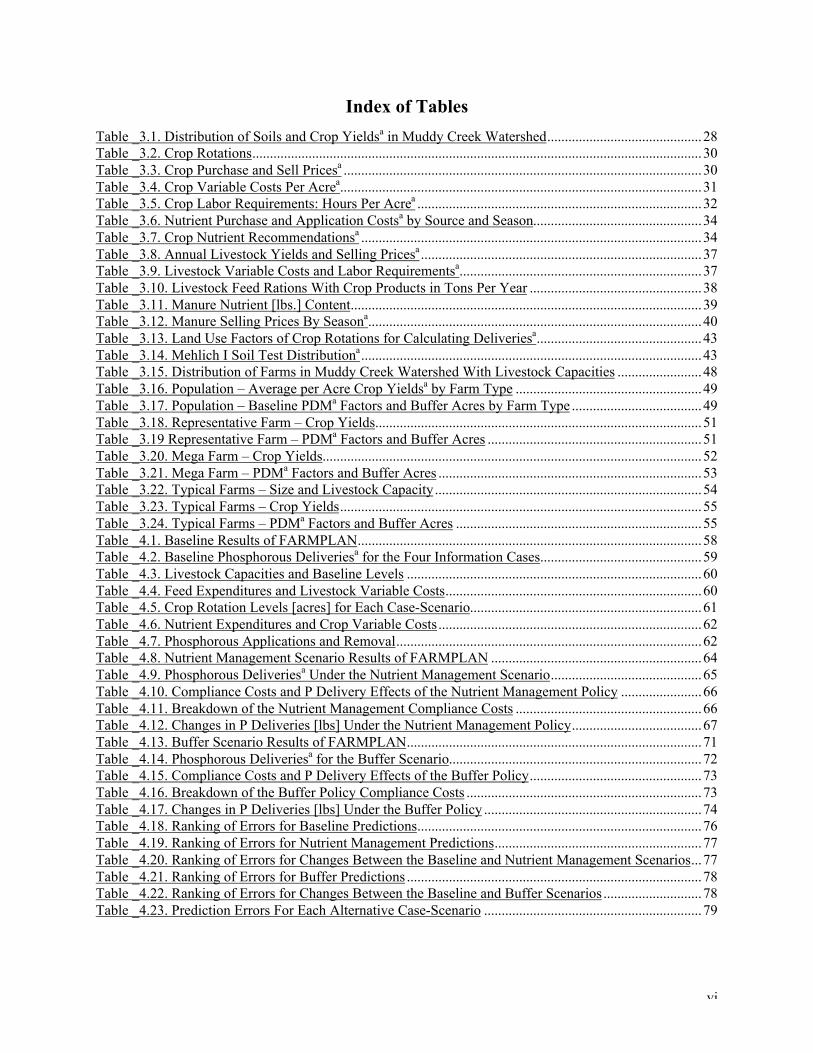
Table _3.1. Distribution of Soils and Crop Yieldsa in Muddy Creek Watershed............................................28Table _3.2. Crop Rotations................................................................................................................................30Table _3.3. Crop Purchase and Sell Pricesa ......................................................................................................30Table _3.4. Crop Variable Costs Per Acrea.......................................................................................................31Table _3.5. Crop Labor Requirements: Hours Per Acrea .................................................................................32Table _3.6. Nutrient Purchase and Application Costsa by Source and Season................................................34Table _3.7. Crop Nutrient Recommendationsa .................................................................................................34Table _3.8. Annual Livestock Yields and Selling Pricesa ................................................................................37Table _3.9. Livestock Variable Costs and Labor Requirementsa.....................................................................37Table _3.10. Livestock Feed Rations With Crop Products in Tons Per Year .................................................38Table _3.11. Manure Nutrient [lbs.] Content....................................................................................................39Table _3.12. Manure Selling Prices By Seasona...............................................................................................40Table _3.13. Land Use Factors of Crop Rotations for Calculating Deliveriesa...............................................43Table _3.14. Mehlich I Soil Test Distributiona.................................................................................................43Table _3.15. Distribution of Farms in Muddy Creek Watershed With Livestock Capacities ........................48Table _3.16. Population – Average per Acre Crop Yieldsa by Farm Type .....................................................49Table _3.17. Population – Baseline PDMa Factors and Buffer Acres by Farm Type .....................................49Table _3.18. Representative Farm – Crop Yields.............................................................................................51Table _3.19 Representative Farm – PDMa Factors and Buffer Acres .............................................................51Table _3.20. Mega Farm – Crop Yields............................................................................................................52Table _3.21. Mega Farm – PDMa Factors and Buffer Acres ...........................................................................53Table _3.22. Typical Farms – Size and Livestock Capacity............................................................................54Table _3.23. Typical Farms – Crop Yields.......................................................................................................55Table _3.24. Typical Farms – PDMa Factors and Buffer Acres ......................................................................55Table _4.1. Baseline Results of FARMPLAN..................................................................................................58Table _4.2. Baseline Phosphorous Deliveriesa for the Four Information Cases..............................................59Table _4.3. Livestock Capacities and Baseline Levels ....................................................................................60Table _4.4. Feed Expenditures and Livestock Variable Costs.........................................................................60Table _4.5. Crop Rotation Levels [acres] for Each Case-Scenario..................................................................61Table _4.6. Nutrient Expenditures and Crop Variable Costs...........................................................................62Table _4.7. Phosphorous Applications and Removal.......................................................................................62Table _4.8. Nutrient Management Scenario Results of FARMPLAN ............................................................64Table _4.9. Phosphorous Deliveriesa Under the Nutrient Management Scenario...........................................65Table _4.10. Compliance Costs and P Delivery Effects of the Nutrient Management Policy .......................66Table _4.11. Breakdown of the Nutrient Management Compliance Costs .....................................................66Table _4.12. Changes in P Deliveries [lbs] Under the Nutrient Management Policy.....................................67Table _4.13. Buffer Scenario Results of FARMPLAN....................................................................................71Table _4.14. Phosphorous Deliveriesa for the Buffer Scenario........................................................................72Table _4.15. Compliance Costs and P Delivery Effects of the Buffer Policy.................................................73Table _4.16. Breakdown of the Buffer Policy Compliance Costs ...................................................................73Table _4.17. Changes in P Deliveries [lbs] Under the Buffer Policy ..............................................................74Table _4.18. Ranking of Errors for Baseline Predictions.................................................................................76Table _4.19. Ranking of Errors for Nutrient Management Predictions...........................................................77Table _4.20. Ranking of Errors for Changes Between the Baseline and Nutrient Management Scenarios...77Table _4.21. Ranking of Errors for Buffer Predictions ....................................................................................78Table _4.22. Ranking of Errors for Changes Between the Baseline and Buffer Scenarios ............................78Table _4.23. Prediction Errors For Each Alternative Case-Scenario ..............................................................79

1
Chapter 1 Agriculture, Phosphorous and Water Quality
1.1 Introduction
Over the last three decades the United States has improved the quality of its waters byusing changes in technology, and production and consumption practices to control pollution from
industrial and municipal sources. However, 40% of surveyed water bodies do not meet fishing
and swimming use standards (U.S. Environmental Protection Agency (EPA), 1997a). Statesreport that nonpoint source (NPS) pollution is the leading remaining cause of water quality
problems (EPA, 1997b), and agriculture has been identified as a major source of NPS pollution
in U.S. lakes and rivers that do not meet water quality goals (National Research Council, p.26).Nutrients and sediment are cited as the leading NPS pollutants (EPA, 1997a).
The Chesapeake Bay is a prime example of a water body that has been impaired bynutrients from agriculture. Research beginning in the late 1970’s discovered that nutrient over-
enrichment and toxic pollution were causing the degradation of fish, Bay grasses, and other
aquatic life (Chesapeake Bay Program, 2001). Since 1983 the Commonwealth of Virginia andits partners in the Chesapeake Bay Program—Maryland, Pennsylvania, the District of Columbia,
the Chesapeake Bay Commission, and the U.S. Environmental Protection Agency—have beendeveloping and implementing methods to restore the Bay’s living resources. Agriculture
contributes 49% of phosphorous (P) entering the Bay (Chesapeake Bay Program 2001), leading
Virginia and its partners to target agriculture for nutrient control. The partners agreed to developtributary-specific strategies in order to reduce P loads—mass or quantity of P—in the Bay by
40% of 1985 levels (Chesapeake Bay Program, 2001). Included in the tributary strategies arepermanent caps on P, so that despite population growth in the watershed, and the associated
increases in municipal wastewater, nutrients entering the Bay will remain at the target of 40%
below baseline. In addition to the Chesapeake Bay Program’s findings, the EPA includedVirginia’s portion of the Bay and several tidal tributaries on the federal list of impaired waters
based on the state’s failure to meet dissolved oxygen and aquatic life use standards. In addition,the EPA has proposed the implementation of a total maximum daily load (TMDL) regulatory
program under Section 303(d) of the Clean Water Act, which may affect nutrient pollution in
many watersheds.Phosphorous and nitrogen (N) are naturally occurring elements in soils that are essential
to plant and animal growth. Submerged aquatic vegetation requires nutrients for growth, and, in
2
turn, filters sediment and provides food, habitat, and dissolved oxygen for other living resources.
Excessive nutrient loads in surface-water bodies lead to accelerated eutrophication.Eutrophication is the process by which a body of water becomes enriched in dissolved nutrients
that stimulate the growth of aquatic plant life usually resulting in the depletion of dissolvedoxygen. Eutrophication caused by excess nutrients can affect aquatic systems by changing their
plant species, or limiting their use for fisheries, recreation, industry, or drinking (Campbell and
Edwards, National Research Council). Soil erosion from agricultural land reduces the use ofwater resources by clogging the receiving water bodies with excessive sediments and impairing
the natural habitat of aquatic plant and animal life. Sediment is also a carrier of many pollutants,including nutrients (Novotny and Olem), and over 90% of nutrient losses are associated with soil
loss (Alberts, Schuman, and Burnwell). In addition to sediment, nutrients can be transported
from topsoil by runoff or groundwater. Runoff is the portion of precipitation on land thatultimately reaches streams, and groundwater is subsurface water that has percolated through the
soil system. Phosphorous is not particularly mobile in soils, and phosphate ions do not
leach—the process by which pollutants enter groundwater—readily (Novotny and Olem).Phosphorous is held tightly by soil particulates and organic matter, with only a small amount of
P occurring in solution (Novotny and Olem).In this study sediment is viewed solely as a vehicle for P transport, and N is not
considered. Phosphorous is singled out as the pollutant of concern in this study because it is
considered the nutrient limiting growth of aquatic vegetation in most surface waters (Daniel etal.). Phosphorous is thus the most important (EPA, 1988) and easiest (Daniel et al.) nutrient to
manage for controlling accelerated eutrophication in freshwater lakes.
1.2 Agro-Pollution
Agriculture has pervasive effects on soil, air, water, plants, and animals. Sediment andnutrient runoff and/or leaching are residuals of agricultural activity. Agricultural land
disturbances can increase erosion rates by two or more orders of magnitude (Novotny and
Olem). Because sediment runoff is a vehicle for the transport of nutrients and other pollutants,soil disturbances also increase the delivery of these pollutants. Loadings of these pollutants also
depend on stochastic weather events, soil and slope characteristics of the watershed, and land use

3
decisions of the farmers. Land use decisions that affect potential pollution include livestock
management, crop rotations, and farming technology such as tillage methods. Many contemporary livestock operations can be considered intensive systems. They are
characterized as having excess nutrients generated on the farm (Beegle and Lanyon), meaningthey have an insufficient amount of cropland on the farm to utilize the amount of nutrients
generated by the livestock (Mostaghimi et al.). Traditionally farms of this nature have used land
application of manures as both a fertilizer and a means of disposal (Novotny and Olem). SomeNPS pollution control policies include limiting manure applications to the amount required to
meet P use by the crop.
1.3 Controlling Agro-Pollution
1.3.1 Introduction
Section 319 of the Clean Water Act charges states and tribes with setting water quality
standards and developing nonpoint source pollution-control programs to meet them. In dealingwith pollution from agriculture, states have mostly relied on education, technical assistance, and
voluntary cost-shared management practices (Malik, Larson, and Ribaudo). The federal
government does provide support for conservation efforts. For example, the ConservationReserve Program is administered by the U.S. Department of Agriculture (USDA) and provides
funding to farmers who establish long-term, resource-conserving covers on eligible farmland.The Environmental Quality Incentives Program, administered by the USDA, provides technical,
educational, and financial assistance to eligible farmers and ranchers to address water and soil
concerns. Many states such as Wisconsin, Virginia, Florida, and North Carolina work with theUSDA programs in addition to providing cost-share programs of their own. Virginia
implemented the Conservation Reserve Enhancement Program which, as the name suggests, is
an enhancement to the USDA program. Through the program, Virginia is calling for theplanting of 22,000 acres of riparian buffers and filter strips in the Chesapeake Bay watershed.
Using federal and state funds the program provides rental and cost-share payments to helpfarmers participate. The Virginia Agricultural Best Management Practices Cost-Share Program
also supports using various practices in conservation planning to treat animal waste, cropland,
pastureland and forested land.
4
1.3.2 Best Management Practices
A best management practice (BMP) can be defined as “a practice or combination of
practices that is determined by a state or designated area-wide planning agency to be the mosteffective and practicable (including technological, economic, and institutional considerations)
means of preventing or reducing the amount of pollution generated by nonpoint sources to a
level compatible with water quality goals.” (Soil Conservation Society of America) Thiscomprehensive definition contains two important criteria, the ability to meet water quality goals
and practicality. Each BMP can be categorized as either managerial or structural, and as source
reduction or transport interruption. Managerial practices involve production decisions that donot require significant capital or alterations of land use; they include the selection of crop and
tillage methods, and nutrient application rates and methods. Structural practices involve thealteration of land or land use (e.g. terraces and buffers), or the construction of devices (e.g.
fences and manure storage facilities). The selection of BMPs is related to the pollutant(s) being
controlled, the level of desired reduction, activities contributing to the pollution, and site-specificcharacteristics such as climate and topography (Bosch and Wolfe). The two BMPs that are
examined in this study are nutrient management and buffers.
1.3.3 Pollution Control Policies
Two pollution-control policy options are design and performance standards. Design
standards for agricultural sources involve regulating the ways farmers manage their land, and, in
the case of nutrient losses, can include restrictions on the levels, timing, and forms of nutrientapplications (Abler and Shortle). Design standards allow policymakers to focus on a small
number of activities that contribute pollution, and develop methods or restrictions that will meetthe policy objectives. Design standards can be efficient—achieve the chosen goal at least
resource cost—because they feature low monitoring costs and can provide a way to save
information costs among polluters (Bohm and Russell). Performance standards involveregulating an observable outcome of the polluter’s decisions (Abler and Shortle). Under a
performance standard the farmer is given the decision of how to meet the objective.Performance standards can be useful when multiple activities are known to contribute pollution,
and the costs of controlling pollution vary among activities within the farm (Bohm and Russell).
Given the flexibility, farmers can select the BMPs that best fit their objectives and constraints.

5
Although performance standards can lead to lower compliance costs, the administrative and
enforcement costs required to implement them can be high (Abler and Shortle).
1.4 Evaluating Policies
1.4.1 Introduction
Policy design is an exercise in problem solving. Goals and objectives must be set,
consequences and assumptions identified, and the decision making process structured so that aconclusive outcome is reached. When evaluating policies to control agricultural pollution, the
analyst attempts to estimate pollution reductions and the costs to achieve them, which areultimately outcomes of the landowners’ responses to the policy. These responses are observed
through production decisions, which will in turn affect farm revenues and costs, and pollutant
loads. To structure the analysis, the analyst must specify how the farms will be represented andhow costs and pollutant loads will be measured. In order to specify the farm representation, the
analyst must first determine the level of information to include. That is, the analyst mustdetermine the characteristics that will affect production decisions, revenue and costs, and
pollutant deliveries.
1.4.2 Spatial Information
Nonpoint source pollution has its name because loads from one point can have multipleentry points to a water body and each entry point can receive loads from multiple origins. This
diffuse nature indicates that many factors contribute to the transport of pollutants. Similarly,variations in physical characteristics affect crop yields and production decisions such as land use
and inputs leading to variations in costs and revenues across farms. Attributes that can
contribute to potential P deliveries and the costs of reducing them can be categorized as: 1)socioeconomic characteristics of the farm, 2) physical characteristics of fields belonging to the
farm, and 3) location of the fields. Because they are site specific, these attributes are referred toas spatial characteristics and the knowledge of them as spatial information. Socioeconomic
characteristics are those that are determined by the land manager and are not fixed temporally;
they include farm and field boundaries, livestock facilities, and crop selection. Livestockfacilities include structures that determine capacity, such as poultry houses and milking parlors,
as well as those for feeding operations and manure storage. Farm type is a term that is used toclassify farms of similar size and primary output (e.g. small dairy and medium beef-with-

6
poultry). Physical characteristics of the field change very slowly and consist of soil map unit,
slope, and slope length. These characteristics contribute to the transport of pollutants to the edgeof the field. However, a field’s location relative to receiving waters also determines deliveries to
the water body. The term location is used to refer to a field’s distance to surface water and theslope, slope length, and crop cover of fields that are down slope and between the source field and
the receiving waters—intervening fields. Therefore, when estimating the potential for P
deliveries from a farm it is imperative to consider its location relative to receiving waters and anyintervening fields.
1.4.3 Farm Descriptions
The water quality literature (e.g. Soranno, Hubler and Carpenter; Just and Antle; Feuzand Skold; Braden et al.) contains theoretical and empirical studies that have attempted to answer
the questions How much spatial information is needed to set policy? and How to model the
spatial characteristics? Preckle and Senatre and Wu and Segerson found that most studies onfarm policy have used representative farms based on aggregate averages for a county or region.
Such representative farms assume that all farms within the study region are endowedhomogeneously and will respond identically to economic and policy signals. Because averaging
data implicitly assumes that surplus resources on one farm are available for use on another farm
for which those resources are limiting, using averages can overstate production and/orproduction possibilities (Feuz and Skold). Wu and Segerson and Opaluch and Segerson
determined that this approach will lead to biased estimates of pollution and pollution reductioncosts. Feuz and Skold addressed this problem by developing a typical farm for each class of
farms, with corresponding proportions of resource endowments, yields, and technologies.
Carpentier, Bosch and Batie showed that incorporating site-specific information could allow forthe targeting of farms with lower costs of complying with a nitrogen runoff control policy.
1.4.4 Estimating Nonpoint Source Pollution
Spatial variation of physical characteristics and the complexity of the soil P cycle makemeasuring P movement and loads difficult. Researchers have developed many tools—e.g.
GLEAMS (Leonard, Knisel and Still), AnnAGNPS (Theurer, Bingner and Cronshey) and
ANSWERS (Bouraoui and Dillaha)—in an attempt to estimate NPS pollution from agriculture.Federal and state agencies have been working on P-index systems that will allow analysts to

7
identify high risk areas for P pollution based on site-specific conditions. Virginia has one such
index (Mullins et al., 2002a and 2002b) that is used in this study. Tools to estimate soilmovement are also used because of the importance sediment has in the transport of P. The
Universal Soil Loss Equation (USLE) is one such tool that estimates average annual soil lossfrom a specified area. The development of geographic information systems (GIS) has allowed
for advanced application of the USLE. Sediment-routing functions can estimate the amount of
an area’s soil loss that will reach surface waters. As was implied in section 1.1, and will befurther explained in section 2.4, P can be broadly classified as particulate or soluble. Section 1.1
also noted that P loads can be found in surface- and ground-waters. This study estimates theloads of both particulate and soluble forms of P in surface water.
1.4.5 Estimating Costs
The decision to implement a policy depends on the expected control costs of meeting the
quality standard. Control costs can be classified as compliance costs or transaction costs(Tietenberg). Transaction costs are incurred by watershed stakeholders, including taxpayers, via
government agencies and include policy design, monitoring, and enforcement costs. Compliancecosts for policies directed at agriculture are incurred by the farmers and include the costs of
infrastructure and planning, increased variable costs, and the decrease in revenue from the
elimination of profitable enterprises—opportunity costs. Compliance costs of a policy are afunction of: 1) the degree of flexibility farmers have to meet pollution requirements, 2) the level
of information farmers have about the costs and benefits of alternative practices, and 3) the levelof information used by policymakers to design the policy. It is foreseeable that a model that
makes poor estimates of costs might lead to a poor choice of policy. The accuracy of a model’s
cost estimate is defined as the degree of conformity to the true value that would be experiencedby farmers if the policy were implemented.
1.5 Problem Statement
1.5.1 Introduction
Nutrient runoff from agriculture is at the forefront of water quality discussions. In thestate of Virginia, population growth and the associated increases in municipal wastewater, along
with the threat of EPA regulations, will increase the need for P reductions in order to meet andmaintain water quality standards for the Chesapeake Bay. Evidence in the literature (Braden et

8
al.; Schwabe; Bosch, Pease and Stone) continues to suggest that spatial characteristics should be
considered when designing policies to control nonpoint sources of water pollution. Spatialcharacteristics affect both the decisions made by farmers and the transport of nutrients. Spatial
information can be expensive to collect and the evidence is not conclusive in determining whatlevels of information should be used for analyzing specific design standards. Historically studies
have used both representative farm models and regional or national-scale models (Bosch, Pease
and Stone). Regardless of the geographic scale, the model must be able to link the spatialattributes and economic parameters in order to make useful predictions of policy costs and
pollution outcomes.Bosch, Pease and Stone cite a lack of data, complexity and policy relevance as challenges
to incorporating spatial effects into economic analyses of NPS pollution from agriculture.
Historically farm economic data and soil resource data have been collected in separate surveysthat used different sampling designs making them unsuitable for coordination (Antle and Just).
Studies that have collected data coordinating economic and physical characteristics have done so
for only one or a few years, limiting their usefulness in studying farmers’ production responsesto changing economic conditions (Bosch, Pease and Stone). Complexity is an issue for both
economic and pollution analyses. Farmers make decisions over multiple time periods and adjusttheir behavior based on feedback from the physical and economic environment. Variation in
soil, slope and land use make predicting pollution at the source difficult. The diffuse nature of
NPS pollution—various flow paths of pollutants to surface water bodies, dependence on weatherevents, the effects of changes in land use along the flow path, and time lags—complicate the
study of pollution deliveries to water bodies. The issue of policy relevance is that spatiallyexplicit results may not be useful to NPS pollution control agencies because of their specificity
(Bosch, Pease and Stone); that is, they can not be easily generalized in a way to set policy for the
greater area of interest. The conclusion is that economic and pollution outcomes are complexfunctions of temporal and spatial variables for which coordinated data are rare and expensive to
collect, leading to case studies so specific that the generalization of results is difficult if possible.Research in this area will help analysts decide what spatial detail is warranted for the analysis of
a given policy.
Different types of practices could require different levels of information for accurateanalysis. Source reduction practices might not need location information since they aim to

9
reduce the production of pollutants rather than increasing interception of pollutants. The analysis
of transport interruption practices might need location information because the location of suchpractices determines effectiveness. The cost and effectiveness of other practices, such as nutrient
management, are more dependent on livestock production, and would likely require moresocioeconomic information to estimate responses.
1.5.2 Levels of Information
This study models a watershed and its farms using four levels of spatial information. The
first level is the simplest case and the levels get progressively more complete in cases 2 – 4.1. The first level of information consists of an estimate of the average farm. Physical
data and expert opinion on the general description of farms in the watershed are used to define asingle representative farm.
2. The second level of information includes complete inventories of soils and livestock
facilities in the watershed that are incorporated into a single “mega” farm.3. The third level of information contains more extensive expert knowledge on the
distribution of socioeconomic characteristics than do the representative and mega farm cases.The additional information is used to define a set of typical farms that are described by averages
of the resources of the corresponding farm type.
4. The fourth, and most complete, level of information considers the population of farms.In this case, all the socioeconomic, physical, and location characteristics of each farm are
assumed to be known and are explicitly defined in the economic and physical models.Because the population comes closest to containing “complete” information, it is used as
the benchmark to which the predictions of the three alternative information cases are compared.
Each of these cases is used to estimate compliance costs and P reductions for each of the twodesign standards, nutrient management and buffers. The accuracy of predictions made by the
three alternative cases is defined as their degree of conformity to the population’s estimates.
1.6 Objectives
The goal of this study is to evaluate how spatial information affects the accuracy of
estimates of economic and physical responses to policies that seek to control NPS pollution fromagriculture. Specifically, the objective is to estimate the accuracy of predicted compliance costs

10
and changes in P deliveries of mandatory buffer installation and mandatory nutrient management
under the three alternative levels of information relative to the population.
1.7 Propositions
Two propositions are made concerning the results. Proposition 1 is that level 3, the set oftypical farms, will yield the most accurate predictions of costs and pollutant reductions relative
to the population; followed by level 2, the mega farm, and then level 1, the representative farm.
Proposition 2 is that the errors will be greater for the scenario of buffers than nutrientmanagement. The first proposition follows from the literature (Feuz and Skold; Wu and
Segerson; and Opaluch and Segerson) regarding representative and typical farm representationsand prediction biases. The second proposition is based on buffers being a transport interruption
practice, the effectiveness of which is dependent on location relative to surface water. Therefore,
the omitted spatial information will have a greater impact on estimates. The details of thepractices are described in chapters 2 and 3.
1.8 Thesis Procedures and Organization
For each information case, an economic model is used to estimate the profit maximizing
levels of inputs, outputs, and net revenue at the farm and watershed levels for the baselinescenario, which imposes no restrictions related to P deliveries. Crop and tillage decisions are
used as inputs for the physical model, which estimates the baseline P deliveries of each farm and
the watershed. The models will be run two more times, once for each policy scenario—nutrientmanagement or buffers. The aggregate net revenues of the watershed, as estimated by the
information cases, for each of the constrained trials are subtracted from the baseline net revenues
to determine compliance costs, while the quantity of P delivered to the watershed outlet issimilarly compared to measure the effectiveness of the policies in reducing P loads. Estimates of
net revenue, compliance costs, P deliveries, and P changes are been made for each informationcase under the baseline, nutrient management policy, and buffer policy. The estimates of those
measurements for each of the alternative information scenarios are compared to those of the
population case to determine their prediction accuracy.This study is not designed to accurately predict P deliveries. However, much effort was
made to include validated techniques and coefficients in the P delivery model. Because the same

11
P delivery model is used across all policies and information cases, the differences in deliveries
across information cases and policy scenarios will be more accurate than absolute values. Thedifferences in deliveries are of most importance in this study.
This thesis is organized to present to the reader the role of spatial information inanalyzing and setting policies to control NPS pollution from agriculture. Chapter 2 presents a
conceptual framework for modeling farms and watersheds and for using those models to estimate
compliance costs and P reductions. Chapter 2 also describes the conceptual framework ofnutrient management and buffers. Chapter 3 describes the empirical application of the
framework presented in Chapter 2. The Muddy Creek watershed is introduced and the collectionof its data explained. The remainder of the chapter outlines how the data were used to construct
the information cases and their use in the economic and physical models. Chapter 4 provides a
discussion of the responses to the policies estimated by the models under the four informationcases. Chapter 5 discusses the conclusions, implications of the results, and the need for future
research.

12
Chapter 2 Conceptual Framework
2.1 Introduction
With many of the gains from the control of point sources of water pollution havingalready been made, scientists and policymakers continue to focus on nonpoint sources, especially
agriculture. When evaluating policies, policymakers and economic analysts attempt to predict
landowner responses. Two primary responses concerning policymakers are pollution reductionsand the costs of achieving them. In order to estimate these responses, the analysts must model
the watershed and the farms within it. These models purport to predict the decisions that the
landowners will make in order to achieve their own goals when faced with resource constraints,market conditions, and production or environmental regulations; and the economic and physical
outcomes that follow. Farm resources and enterprises such as livestock types and facilities, andphysical characteristics such as soil map units and slope, affect the potential for pollution and its
control costs. Accurate prediction of responses to policies requires the incorporation of these
characteristics into a spatially-based model.The analysis of policies whose objectives are to control P loads from agriculture to
surface water can be separated into four components: characterization of the watershed,estimation of the compliance costs, P delivery predictions, and alternatives for controlling P
deliveries. Watershed characterization consists of a specific level of information used to capture
spatial variability. Estimating compliance costs requires specification of an economic model thatis consistent with the watershed characterization. Predicting P deliveries requires a physical
model that can either be separate from or integrated into the economic model and must accountfor the behavior of P in the natural environment. Existing physical models use various means to
predict pollution flows and operate at different geographic scales. Consideration of alternatives
for controlling P requires the analysis of various policies.
2.2 Characterizing Watersheds for Policy Impact Studies
2.2.1 Micro-parameter Models
In the context of a watershed each farm can be considered a micro unit, and, in the
context of a farm, each field can be considered a micro unit. The physical characteristics of afield determine its output capacity for crops, while size and livestock facilities determine the
output capacity of the farm—both crops and livestock. The relationship between inputs and

13
outputs, and pollution depends on the fixed characteristics of the micro unit (Hochman and
Zilberman, 1978). Econometric micro-parameter models allow the use of data observed fromactual farms to estimate the farmers’ responses to policies and the environmental impacts of
those responses (Bosch, Pease and Stone). Models using micro-parameter distributions can beused to model the linkages between agricultural policies and agricultural pollution (Hochman
and Zilberman 1978,1979; Just and Antle; Opaluch and Segerson). Policies can have complex
effects on the joint distributions of output and pollution and inputs and pollution (Just and Antle).Micro-parameter models reflect the joint effects of physical characteristics, land use, inputs,
output, and pollution. In such models the spatial characteristics are assumed to be fixed for eachfarm but are allowed to vary across farms, and the objective of each farmer is assumed to be
profit maximization. The model utilizes the spatial characteristics to determine farm responses
to price and policy signals (Bosch, Pease, and Stone). Adjustments can be made to input andother managerial decisions on how crops and livestock are produced; or they can be made to land
use decisions such as crop mix and structural practices. An advantage to this method is that
quantitative hypothesis testing can be conducted. However, these models require large amountsof physical and economic data. Micro-parameter distribution models can also be used in
conjunction with GIS to analyze NPS pollution problems while recognizing the importance ofsite-specific attributes (Opaluch and Segerson). In cases where data are insufficient to use an
econometric model, mathematical programming can be used to capture the features of the micro-
parameter framework (Carpentier, Bosch and Batie).
2.2.2 Spatial Information
The use of a single representative farm—a hypothetical farm designed to represent many
farms in the study area—fails to capture the heterogeneity of farm objectives and resources (e.g.Feuz and Skold, Wu and Segerson, Preckle and Senatre). The socioeconomic, physical, and
location characteristics of a farm contribute to NPS pollution and control costs (Bosch, Pease,
and Stone; Wu and Segerson; Peng and Bosch; Schwabe; Braden et al.). Socioeconomiccharacteristics are important because they affect resources and production decisions. Livestock
facilities also determine nutrient runoff potential from manure applications (Bosch, Pease, andStone). Physical characteristics of soils are important because they determine both production
possibilities and nutrient transport potential. The potential for nutrient leaching and runoff is
determined by soil water-holding capacity and slope (National Research Council).

14
Location characteristics are important because they determine the delivery of pollutants
from the source field to the receiving waters. For example, N deliveries have been found to behigher for fields located closer to streams and with steeper slopes (Peng and Bosch). When
studying the use of buffers to control N deliveries in North Carolina, Schwabe found thathomogenizing the soil characteristics (slope, erodibility, and drainage intensity) resulted in a
positive bias of N reductions and negative biases of total and per unit compliance costs. A
limitation of the study is that Schwabe considered each county in the study region as a singlefarm. Braden et al. argue that economists have focused on reducing discharges and that
possibilities for the containment of pollutants have gone largely unnoticed. In their discussion ofthe literature, Braden et al. find that most economic models of pollution abatement assume that
emissions and effects are linked by fixed delivery ratios. Braden et al. assert that if damages are
not proportional to discharges then controlling discharges alone will likely be a second-beststrategy, and that to achieve maximum efficiency, practices that intercept the pollutant and
change the delivery ratios must be considered. The Braden et al. study provides a theoretical
framework for reducing pollutant deliveries to water sources that requires consideration of notonly physical characteristics of the site, but relative location as well.
In this study, the four information cases attempt to capture various amounts of the spatialcharacteristics of a watershed. In the case of the representative farm, the hypothetical situation is
that the analyst has data containing the soil inventory, topography, hydrology, field boundaries,
and general land use patterns—i.e. commercial, residential, forest, and agriculture. The analystemploys a local expert to estimate the number of farms and fields in the watershed, the average
size of the farms, and average livestock facilities. The analyst then uses the data containing thephysical characteristics to determine the average physical characteristics of the watershed and
uses them to describe the representative farm. Specifically, the farm is of average size according
to the expert, contains the average soil present in the watershed, has the average livestockfacilities according to the expert, and has average P delivery ratios.
In the case of the mega farm, the hypothetical situation is that the analyst has the datacontaining the soil inventory, topography, hydrology, and general land use, but that expert
knowledge obtained includes complete information on livestock facilities. Farm and field
boundaries and exact farm numbers are unknown. The scenario is similar to that of therepresentative farm, but in this case the analyst uses the additional information on livestock

15
facilities to model the watershed as a single farm. This reduces the potential for biases created
by averaging livestock facilities and land resources, but maintains the bias of aggregatingphysical resources because surplus resources that belong to one “true” farm are now available to
another. This aggregation results in bias because as Feuz and Skold found, many practicesappear profitable from a single enterprise perspective but are less attractive when considered as
part of a whole-farm system. The mega farm retains the bias of the single enterprise analysis
discussed by Feuz and Skold because the constraints imposed by farm boundaries are ignored.The actual system of farms in the watershed is similar to their whole-farm system because the
limitations of farm boundaries and farm resources are imposed.For the case of the typical farms, the hypothetical situation is that the analyst has the data
containing the soil inventory, topography, hydrology, field boundaries, and general land use
patterns. However, differing from the representative and mega farm cases, the analyst employsmore expert knowledge or surveys to obtain more complete information regarding the
distribution of farm sizes and livestock facilities. Information on correlations between farm
types and location and resources may be included. From this additional information, the analystis able to construct a set of typical farms that better represents the distribution of farms in the
watershed. Preckle and Senatre found in their study of commodity programs that a subset ofheterogeneous farms predicted more subtle changes in farm responses than a single farm. In
particular, the single farm grossly overestimated program participation, government payment
outlays, and corn supply response.As described in Chapter 1 the case of the population of farms assumes the analyst has
“complete” information on all socioeconomic, physical, and location characteristics. It istherefore assumed that the economic and physical models will make reasonable estimates of
farm responses to the applied policies.
2.3 Compliance Costs
Compliance costs are the costs of achieving the objectives of a policy once the policy has
been implemented (Tietenberg). They do not include enforcement and other administrativecosts, which are considered transaction costs. Compliance costs are measured as the reduction in
net revenue after implementation of the policy and are estimated as:

16
 Â= =
-=J
j
J
jjjjji xcxcCC
1 1
1100 , (2.1)
where CCi is the compliance cost of the ith farm, 0jc is the net return on activity j under the
baseline, and 0jx is the level of activity j. Similarly, 1
jc and 1jx are the net return and level of
activity j after a pollution-control standard has been imposed.
The accuracy of cost estimates is defined as the degree of conformity to the true value ora designated standard. The population information case is considered the benchmark for
estimates as it is considered the complete information case. Compliance costs for individualfarms are aggregated to the watershed level for comparison. The effects of spatial information
on the cost predictions are evaluated by how predictions from each of the alternative information
cases compare to predictions made from the population case and are estimated as:
100*Pop
PopAltAlt
CC
CCCC -=E (2.2)
where EAlt is the prediction error of an alternative case, and CCPop and CCAlt are the compliancecosts predicted by the population and alternative cases, respectively. Equation 2.2 estimates the
prediction error of a model as the difference between the compliance costs estimated under thepopulation case and an alternative case as a percentage of the compliance costs of the population
case. The size and sign of the prediction errors of each information case are compared to
evaluate the effects spatial information has on the estimation of compliance costs under thebaseline and the nutrient management and buffer policy scenarios.
2.4 Phosphorous Delivery
2.4.1 The Phosphorous Cycle
The properties and behavior of P in soils and water are complex. Understanding theprocesses by which P moves across geographic space and interacts with the chemical and
biological environment is essential to modeling P deliveries to surface water bodies.Phosphorous can be classified as particulate or soluble and as organic or inorganic.
Particulate P can be organic or inorganic while soluble P is mostly inorganic. Soluble P is found
in the soil solution and is available for uptake by plants and transport by leaching or surfacerunoff. An equilibrium exists between the levels of particulate and soluble P with the

17
concentration of soluble P being controlled by the concentration of particulate P (Campbell and
Edwards, National Research Council). Inorganic, particulate P can be further classified assorbed P, primary P minerals, or secondary P minerals. The P cycle includes interactions and
transformations occurring through a variety of physical, chemical, and microbiological processesthat determine the forms of P, its availability to plants, and its transport in runoff or leaching
(Campbell and Edwards). Complex processes that are influenced by many characteristics of the
soil, water, plant, and atmospheric environment transform P from one form to another. PrimaryP minerals originate from the weathering of soil minerals and other more stable geologic
materials. Dissolution is the process by which primary and secondary P minerals aretransformed into soluble P, while precipitation is the process by which soluble P is transformed
into secondary P minerals. Adsorption is the process by which soluble P is chemically bound to
reactive soil constituents, while desorption is the opposing process that transforms sorbed P intosoluble P. Finally, mineralization is the biological conversion of organic P to mineral P, and
immobilization is the conversion of mineral P to microbial biomass. These opposing processes
occur continuously and simultaneously. At any given time, most of the P in soils is normally inrelatively stable forms that are not readily available to plants or dissolved in water, resulting in
relatively low concentrations of dissolved P in the soil solution (Campbell and Edwards).Phosphorous that is taken up by plants can be removed in the harvest of crops, recycled
on the soil surface as animal waste from grazing animals, or returned to the soil in plant residues
remaining on the surface and as decaying root mass. P can be transported from the soil system insoluble form or adsorbed to eroded sediment. P that is not transported to receiving waters can
become trapped in one of several sinks: deposition with sediment in low areas of the landscape,deposition or plant uptake in field borders, treatment wetlands, and riparian zones. All of these
potential sinks have upper limits to the quantity of P that can be retained and may be more or less
effective depending on a range of conditions (Campbell and Edwards).Because P is essential to plant growth, it is frequently applied to meet crop needs. A
portion of the applied P becomes unavailable to crops because of adsorption and precipitation;therefore, applications may exceed crop requirements leading to a buildup of P in the soil
system. The accumulation of P will eventually lead to a new equilibrium level of dissolved P. In
some cases manure is applied to meet crop N needs; however, the ratio of N to P in manure isless than crop requirements, which can also result in excess applications of P. Adding fertilizer
18
P, commercial or manure, to crops can result in excess P that is available for transport to
receiving waters (Campbell and Edwards, Beegle and Lanyon). Impacts of P on aquatic systemsare dependent on the form of P delivered as well as relationships between plants and water.
Some forms are available for immediate use by aquatic plants while others can become adsorbedby bottom sediments, stored, and later released into the water column (Campbell and Edwards).
Adsorbed P can become a pollutant when it is transported to receiving waters along with
sediment P, while soluble P can be directly transported in the runoff. Mineral P, or P that hasbeen precipitated, is not as susceptible to transport by runoff alone and is less susceptible than
adsorbed P which is associated with fine soil particles (Campbell and Edwards).
2.4.2 Modeling Phosphorous Deliveries
A variety of tools and models have been developed to estimate sediment, runoff and
nutrient movement. ANSWERS-2000 (Bouraoui and Dillaha) and AnnAGNPS (Theurer,
Bingner and Cronshey) are two watershed-scale simulation models used to predict sedimentloads. Although they are distributed at the field level and are capable of simulating watersheds
up to 10,000 hectares in size, they require a large number of cells to adequately describe thespatial variation and also require a large amount of computer time to run (Veith). An alternative
to simulation models is an integration of mathematical models and indexes. This study uses the
Universal Soil Loss Equation (USLE) (Schwab et al.), sediment and runoff routing functions(Veith), and the Virginia Phosphorous Index (Mullins et al., 2002b) to estimate erosion, sediment
deliveries, sediment P concentrations, runoff, and runoff P concentrations. Combining thesetools allowed a relative comparison of P deliveries to a watershed outlet. The various
components are built into a GIS that represents the watershed using 30-meter cells. These cells,
being smaller than field size, allow the model to capture spatial variability of soils andtopography within the fields. The total amount of P delivered to the watershed outlet can be
separated into two components, sediment-P (SP) and runoff-P (RP). Sediment-P is a function of
erosion, P concentration, and a delivery factor. The delivery factor captures the physicalcharacteristics of the area and is a function of slope, slope length, and land use of intervening
land units (i.e. cells or fields). Runoff-P is a function of runoff volume, P concentration, and adelivery factor. The function for the runoff delivery factor is the same as the sediment delivery
factor except that the land use coefficients are different—because land use affects the movement
of sediment and runoff differently.

19
The P delivery model (PDM) used in this study consists of two equations, 2.3 and 2.4,
that calculate SP and RP, respectively. These two equations are based on the equations in theVirginia P-Index (P-Index) that estimate the erosion and runoff risk factors. Using the GIS these
calculations are made at the 30-meter1 cell level, the results are summed over all the cells in eachfield, and from there they are summed over fields in a farm and over the entire watershed.
SPj = rjYj (2.3)
where
SPj = sediment-P yield of cell j [lbs]
Yj = sediment yield of cell j [million lbs]rj = sediment-P coefficient of cell j [parts per million (ppm)];
and
RPj = sj(ROY)j + APj * APFj (2.4)
where
RPj = runoff-P yield from cell j [million lbs]ROYj = runoff yield of cell j [million lbs]
sj = runoff P concentration coefficient of cell j [ppm]
APj = P applied to cell j [lbs]
APFj = product of fertilizer source and application factors.Sediment-P is the quantity of P attached to sediment that is delivered to the watershed outlet,
sediment yield (Y) is the quantity of sediment delivered to the watershed outlet, and the
sediment-P coefficient (r) measures the concentration of P in the sediment. Runoff-P estimates
the quantity of soluble-P found in runoff that is delivered to the watershed outlet, runoff yield(ROY) is the quantity of runoff that is delivered to the watershed outlet, and the soluble-P
coefficient (r) estimates the concentration of P in the runoff. The quantity of P applied to fields,
the source of P, and application method are also factors of RP.
Sediment-P and runoff-P at the field level are determined by summing SPj and RPj acrossall the cells in each field. Total-P (TP) is estimated as the sum of SP and RP for each field. The
effectiveness of the NMP and buffers was estimated as the change in TP. The accuracy of thealternative information cases’ estimates of the change in TP was computed in the same fashion
as the compliance costs and is shown in equation 2.5: 1 Calculations made in metric units are converted to English units within the model.

20
100*Pop
PopAltAlt
CP
CPCP -=E , (2.5)
where CP is the difference between TP under the baseline and a policy scenario.
Sediment-P
Sediment yield (Y) was found using a sediment routing function developed by Veith.The function computes the product of gross erosion (A), cell area (a), and a sediment delivery
ratio (d). This method, shown in equation 2.6, accounts for down-slope variations in land use,flow length and steepness.
’=K
kkjjj daAY (2.6)
where
Yj = sediment yield from cell j [million lbs.],
Aj = average annual soil loss of cell j [million lbs/acre],aj = area of cell j [acres],
dk = sediment delivery ratio of cell k [dimensionless], where cell k is in the flow path of
cell j2, andK = number of cells in the flow path of cell j.
Average annual soil loss (A) is found using the USLE. The USLE, shown in equation 2.7, isused for predicting overland soil loss at the cell level. It has been used in other watershed
models (Binger and Braden et al.) and has been shown to be “acceptably accurate in many cases”
for long-term average annual soil erosion (Foster, p.98). A limitation of the USLE is that it doesnot consider the effects of single meteorological events or seasonal variation; however, the
results do estimate the long-term impacts of established management practices (Veith).
Aj = RjKjLjSjCjPj (2.7)
where Aj = average annual soil loss of cell j [million lbs/acre],
Rj = combined rainfall and runoff erosivity of cell j,Kj = soil erodibility of cell j,
Lj = slope length factor of cell j,
2 A cell is considered to be in its own flow path.
21
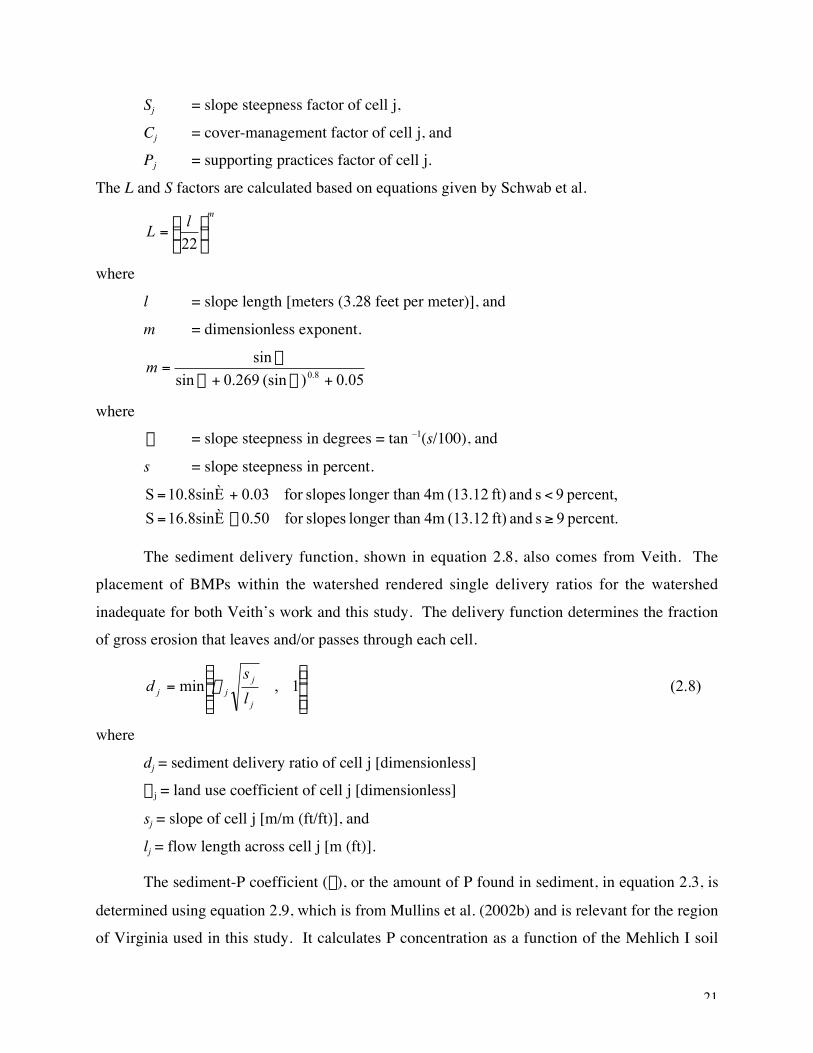
Sj = slope steepness factor of cell j,
Cj = cover-management factor of cell j, andPj = supporting practices factor of cell j.
The L and S factors are calculated based on equations given by Schwab et al.m
lL ˜
¯
ˆÁË
Ê=22
where
l = slope length [meters (3.28 feet per meter)], and
m = dimensionless exponent.
05.0)(sin269.0sin
sin8.0 +Q+Q
Q=m
whereQ = slope steepness in degrees = tan –1(s/100), and
s = slope steepness in percent.
percent. 9 s and ft) (13.12 4mn longer tha slopesfor 0.5016.8sinÈS
percent, 9 s and ft) (13.12 4mn longer tha slopesfor 0.0310.8sinÈS
≥-=
<+=
The sediment delivery function, shown in equation 2.8, also comes from Veith. Theplacement of BMPs within the watershed rendered single delivery ratios for the watershed
inadequate for both Veith’s work and this study. The delivery function determines the fractionof gross erosion that leaves and/or passes through each cell.
Ô
Ô˝¸
ÔÓ
ÔÌÏ
= 1,minj
jjj l
sd a (2.8)
where
dj = sediment delivery ratio of cell j [dimensionless]aj = land use coefficient of cell j [dimensionless]
sj = slope of cell j [m/m (ft/ft)], and
lj = flow length across cell j [m (ft)].
The sediment-P coefficient (r), or the amount of P found in sediment, in equation 2.3, is
determined using equation 2.9, which is from Mullins et al. (2002b) and is relevant for the regionof Virginia used in this study. It calculates P concentration as a function of the Mehlich I soil

22
test value. The Mehlich I is a soil test for the analysis of P, potassium (K), calcium, magnesium,
sodium and micronutrients.
r = 642 + 1.886(Mehlich I) (2.9)
Runoff-PRunoff yield (ROY) is found using equation 2.10, which was developed by Veith and is
an extension of the sediment routing function.
’=K
kkjjj baROROY (2.10)
whereROYj = runoff yield of cell j [million lbs]
ROj = average annual runoff of cell j [million lbs/acre]
aj = area of cell j [acres]bk = runoff delivery ratio of cell k [dimensionless].
The NRCS curve number method is used to determine annual runoff (RO). Curve numbers (U.S.Soil Conservation Service) are identified based on the hydrologic soil group of the field and its
land use description; e.g. row crops, straight row. The curve number is then cross referenced
with average annual runoff which is based on climatic zones. Runoff is given in inches and isconverted to million lbs. per acre.
The runoff delivery ratio (b) is found in equation, 2.11, which is similar to the one used to
derive the sediment delivery ratio. Land use has different effects on the movement of sedimentand runoff, therefore different coefficients are required when calculating the sediment and runoff
delivery ratios.
Ô
Ô˝¸
ÔÓ
ÔÌÏ
= 1,minj
jjj l
sb b (2.11)
where
bj = runoff delivery ratio of cell j [dimensionless]
bj = land use coefficient of cell j [dimensionless]
sj = slope of cell j [m/m]lj = slope length of cell j [m].

23
The runoff-P coefficient (r), or decimal fraction of P found in runoff, in equation 2.4 is
determined using equation 2.12, which is from Mullins et al. (2002a). Like the sediment-P
coefficient it is a function of the Mehlich I soil test.r = 0.3522 + 0.005651(Mehlich I) (2.12).
2.5 Alternatives for Managing Phosphorous Delivery
2.5.1 Nutrient Management
Nutrient management is a managerial, source reduction practice. It is defined by the U.S.
Natural Resources Conservation Service (NRCS) as managing the amount, source, placement,form, and timing of the application of nutrients and soil amendments. When designing a nutrient
management plan, all sources and sinks of nutrients on the farm must be considered with the goalof matching the sources and sinks as closely as possible (Virginia Dept. of Conservation and
Recreation). The focus of a nutrient management plan for a livestock-intensive system is to
identify alternative utilizations of the manure produced in order to minimize nutrient losses whilestill achieving crop yield goals. Allowing that at least some quantity of the manure can be used
as fertilizer on the farm, Bosch and Wolfe note that variation in characteristics, particularly
nutrient content, makes manure difficult to manage. Mostaghimi et al. cite transportation costsas the major obstacle to the use of manure as a nutrient supplement on other farms. In the case
of P, method and placement of fertilizers are more significant than timing in determining P losspotential because of its soil-immobile characteristics (Bosch and Wolfe). Nutrient management
can reduce P losses by 20–90% and is especially effective in controlling P in its highly mobile
soluble phase (Novotny and Olem). Three costs can arise from the implementation of a nutrientmanagement plan. The first is that when applying manure on cropland one nutrient’s
requirements (usually P) will be met before the others (usually N and K) causing the farmer topurchase commercial fertilizer to make up the balance. The second cost is that crop P
requirements will be met before all the manure produced on the farm is disposed, which will
force the farmer to sell the balance. Manure stored in liquid form has low nutrient concentration(see Table 3.11) and a high transportation cost which may mean that sale prices are negative.
The third cost is for plan writing, including soil tests.

24
2.5.2 Buffers
Filter strips are defined by NRCS (2001) as a strip or area of vegetation for removing
sediment, organic matter, nutrients, and other pollutants from runoff. Buffer is commonly usedin the conservation field as a catch-all term for filter strips and other similar practices (e.g.
riparian buffer zones and field borders). The term buffer will be used in this study in place of
filter strips. Buffers are structural, transport interruption practices located between fields andreceiving waters that remove pollutants from surface and subsurface runoff. Buffers remove
pollutants by filtration, infiltration, absorption, adsorption, uptake, volatization, and deposition
(USDA). Filter strips (buffers) work by slowing water velocity (Bosch and Wolfe) and are mosteffective when shallow overland flow, or sheet flow, passes through the strip (Mostaghimi et al.).
The effectiveness of buffers in reducing the delivery of P is difficult to quantify because of thevarious forms P can take and the characteristics of those forms. Estimates for reductions of
soluble P range from 5–50% (Novotny and Olem). Reductions of total-P are likely to be higher
because buffers are 35–90% effective in trapping sediment, which is attached to other forms ofP. The long-term effectiveness of buffers is a concern because as sediment and nutrients
accumulate, large flows from extreme precipitation events may flush the buffer of its loads(Mostaghimi et al.).
Implementing a buffer imposes both direct and indirect costs on the farmer. The indirect
costs are the opportunity costs of taking crop or pasture land out of production. The direct costsare those incurred in establishing and maintaining the buffer itself. Establishing a buffer requires
the purchase of seeds, herbicides and nutrients, and rental and operating expenses for a seeder.Maintenance includes the purchase and application of lime, and the operating costs of a bush
hog.
Government programs are currently in place that provide incentive and/or cost-sharepayments for both of these practices. These payments were not included in the model in order to
isolate the true cost of implementation and because the payments could potentially beunnecessary if the practices are mandated. After the costs of various policies have been
compared, the decision maker can evaluate the usefulness of the BMPs in their existing or
revised state, and the desirability of subsidies.

25
Chapter 3 Empirical Application
3.1 Introduction
The Muddy Creek Watershed in Rockingham County, Virginia served as the case studyfor this project. Located in the Shenandoah Valley, the waters of Muddy Creek flow into the
Shenandoah and Potomac rivers, and eventually into the Chesapeake Bay. Livestock-intensive
farms raising dairy cows, beef cows, and poultry occupy nearly two-thirds of the area. Fivetypes of farms exist in the watershed: dairy, beef, poultry, dairy-with-poultry, and beef-with-
poultry. Poultry operations, including those with dairy and beef operations, raise either broiler
chickens or turkeys. Current practices involve spreading litter and manure to meet crop Nrequirements, but because the ratio of N to P in the litter and manure is less than the ratio of N to
P requirements for crops, applications often exceed crop P requirements.The physical and socioeconomic characteristics of the watershed and its population of
farms were described in four cases of varying spatial information following the discussions in
sections 1.5 and 2.2. A linear programming model, FARMPLAN, written in GAMS (GeneralAlgebraic Modeling System) (Brooke et al.) was used to estimate input and output decisions and
net revenue at the field, farm and watershed levels. A P delivery model, PDM, as outlined insection 2.4, used the physical data and production decisions from FARMPLAN to estimate
sediment-P, runoff-P and total-P deliveries to the watershed outlet. FARMPLAN and PDM were
run for each information case under baseline, nutrient management and buffer scenarios.Following section 2.3 the compliance costs of implementing the nutrient management plan and
buffers were calculated for each case. The compliance costs of each alternative information casewere aggregated to the watershed level and compared to the population’s compliance costs to
determine the prediction errors—equation 2.2. Similarly, the alternative cases’ accuracy in
predicting the change in total-P were estimated using equation 2.5.
3.2 Data
The Muddy Creek Watershed is being used as a case study by an interdisciplinary group
of researchers at Virginia Tech. The group combined resources and expertise in order toadequately describe the watershed’s geography and the characteristics of its farm population.
The data used in this effort came in several forms. The foundation is a digitized data layer that
was provided by the Virginia Department of Conservation and Recreation; it contains land use
26
information, a soil map, and elevation map. A geographic information system (GIS) was used to
store and view the data. Aerial photographs and slides, and orthochromatic photographsprovided by the National Aerial Photograph Program and U.S. Farm Service Agency complete
the data set.Each farm was described by several characteristics. Farm level characteristics consist of
number and size of fields, livestock capacity, manure production potential, and manure storage
capacity. Field level attributes consist of the majority soil map unit present, P concentrations ofsediment and runoff, RKLS factor, and sediment and runoff delivery factors. Potential crop
yields for each field were calculated based on the majority soil (soil map unit) present anddiscounted for slope and rockiness according to the Virginia Agronomic Land Use Evaluation
System (VALUES) guidelines (Donohue, et al.). VALUES restructured and reoriented soil test
recommendations to the best available technology on water quality oriented nutrientmanagement. VALUES was developed out of the concern over the contribution to the decline of
living resources in the Chesapeake Bay made by agricultural activities. The distribution of soils
and their corresponding yields are shown in Table 3.1.
3.3 Farm Model
The production model used in this study, FARMPLAN, is an updated version of
ECONPLAN (Landry, Bosch and Pease). ECONPLAN is a linear programming model writtenin GAMS and has an objective function of profit maximization. ECONPLAN grouped cropland
by soil resource groups. Each soil resource group contains the total acres of soils in a data setwith similar yield characteristics. The primary change made to ECONPLAN for this study was
the use of fields rather than soil resource groups for land use decisions. The use of fields
allowed for the inclusion of more spatial information from the data and the use of the GIS withthe P delivery model. Specifically, the revised model was able to include information regarding
field location, which was used to estimate sediment and runoff delivery coefficients. InECONPLAN there were only six soil resource groups, so the variability in yields was limited. In
this study, using field level data resulted in 23 different yield combinations.
Each farm is described by its fields, livestock capacity, and manure storage capacity. Thefields are described by size (acres) and the majority soil present, which determines the potential
crop yields. The objective of each farm is profit, or gross margins, maximization and the

27
objective function is defined as total gross margins, which equal revenues minus costs. Revenue
sources include sales from livestock activities, crop products and poultry litter. Costs includecrop and livestock variable costs, manure storage, nutrients for crops and their application, feed
for livestock, labor, off-farm disposal of dairy manure, and nutrient management plan writing.FARMPLAN, which is provided in Appendix A, is a distributed micro-parameter model because
livestock facilities and farm boundaries are fixed parameters for each farm while varying from
farm to farm. Similarly, for each field in a farm, size, soil map unit, and slope are fixedparameters, yet they vary from field to field.
FARMPLAN activities are organized into three categories: crops and nutrients, livestockand manure, and BMPs. Full-time labor was assumed to be a fixed resource and its cost is not
included in variable costs. It was assumed that the farm annually has available labor to meet
livestock requirements plus three hours for each acre of crop and pasture land. It was assumedthat the farmer works longer hours in the spring and fall, i.e. during the planting and harvesting
seasons, respectively. Annual available labor was allocated to reflect this. The result is that
27.5% of the annual labor is allocated each to spring and fall, and 22.5% was allocated each towinter and summer. Part-time labor is available at a cost of $7.50 per hour (2001 dollars).
Labor use is a variable indexed over seasons. It is set less than or equal to the sum of seasonalavailable labor and seasonal part-time labor. Annual labor costs are the product of seasonal part-
time labor and 7.5, summed over the seasons.

28
Table 3.1. Distribution of Soils and Crop Yieldsa in Muddy Creek Watershed
Soil Name Acres
CornGrain[bu/a]
CornSilage[tons/a]
RyeSilage[tons/a]
AlfalfaHay
[tons/a]
GrassHay
[tons/a]
Allegheny cobbly fine sandy loam 9.5 110.5 15.6 4.3 3.0 3.6Allegheny fine sandy loam 116.3 130.0 17.8 5.0 3.5 4.3Aquic Udifluvents 260.9 65.0 10.4 1.5 0.0 1.3Berks-Weikert shaly silt loams (slope 15-25%) 66.4 52.0 8.9 2.5 0.0 1.3Berks-Weikert shaly silt loams (slope 7-15%) 12.5 55.3 9.3 2.7 0.0 1.3Craigsville cobbly fine sandy loam 81.8 72.3 11.2 4.3 0.0 1.3Edom silty clay loam 23.9 114.4 16.0 4.4 6.2 4.4Endcav silt loam 39.7 100.0 14.4 3.8 0.0 1.3Fluvaquents 241.9 65.0 10.4 1.5 0.0 1.3Frederick & Lodi cherty silt loams (slope 15-25%) 586.4 104.0 14.9 4.0 5.6 3.4Frederick & Lodi cherty silt loams (slope 7-15%) 172.2 114.4 16.0 4.4 6.2 3.7Frederick & Lodi silt clay loams 19.3 114.4 16.0 4.4 6.2 3.7Frederick & Lodi silt loams (slope 15-25%) 1,278.6 104.0 14.9 4.0 5.6 3.4Frederick & Lodi silt loams (slope 7-15%) 5,188.5 114.4 16.0 4.4 6.2 3.7Frederick & Lodi silt loams (slope 2-7%) 433.1 130.0 17.8 5.0 7.0 4.3Frederick & Lodi silt loams, rocky (slope 15-25%) 165.1 104.0 14.9 4.0 5.6 3.4Frederick & Lodi silt loams, rocky (slope 7-15%) 331.2 114.4 16.0 4.4 6.2 3.7Frederick & Lodi silt loams, rocky (slope 2-7%) 59.2 117.0 16.3 4.5 6.3 3.8Frederick-Rock outcrop complex (slope 15-45%) 85.3 0.0 0.0 0.0 0.0 1.3Frederick-Rock outcrop complex (slope 3-15%) 364.2 104.0 14.9 4.0 5.6 3.4Guernsey silt loam 201.8 130.0 17.8 5.0 7.0 4.3Laidig cobbly fine sandy loam (slope 7-15%) 92.1 88.0 13.0 2.8 0.0 1.3Laidig cobbly fine sandy loam (slope 2-7%) 22.8 90.0 13.3 2.8 0.0 1.3Laidig gravelly fine sandy loam (slope 7-15%) 20.4 88.0 13.0 2.8 0.0 1.3Laidig gravelly fine sandy loam (slope 2-7%) 72.9 100.0 14.4 3.1 0.0 1.3Monongahela cobbly fine sandy loam 115.6 85.0 12.7 2.7 0.0 1.3Monongahela fine sandy loam 168.0 100.0 14.4 3.1 0.0 1.3Rock outcrop-Frederick complex (slope 15-45%) 123.8 104.0 14.9 4.0 5.6 3.4Rock outcrop-Frederick complex (slope 2-15%) 612.0 114.4 16.0 4.4 6.2 3.7Sequoia-Berks silt loams 13.6 110.0 15.5 5.0 3.5 1.6Sequoia-Berks silt loams 85.5 96.8 14.0 4.4 3.1 1.4Sequoia-Berks stony loams 4.5 88.0 13.0 4.0 2.8 1.3Shenval loam (slope 7-15%) 38.1 130.0 17.8 5.0 5.0 4.3Shenval loam (slope 2-7%) 37.3 130.0 17.8 5.0 5.0 4.3Timberville Variant silt loam 61.4 140.0 19.0 5.0 5.0 4.3Wheeling fine sandy loam 5.9 85.0 12.7 5.0 7.0 5.0
a. Yields obtained from Donohue et al.
3.3.1 Crops and Nutrients
Four crops are available for production: corn for grain or silage, rye for silage, alfalfahay, and red-clover orchard grass, which can be used for hay or pasture. The crops can be grown
using conventional or no-till tillage methods, except pasture, which requires no tillage. The set
of crops also includes alfalfa hay establishment, grass hay establishment, buffers and buffer

29
establishment. The buffer is included as a possible BMP. The establishment crops are needed
because, as the name implies, the crops need an initial period of establishment that differs fromthe maintenance period in regards to nutrient requirements, variable costs, labor requirements,
and yields. Alfalfa and grass hay yields during the one-year establishment period are half of theannual yields during the maintenance period. There are sixteen crop rotations, which are shown
in Table 3.2. In the corn-and-rye rotations, the fields are double cropped, meaning that the corn
and rye are planted on the same land at separate times of the year. In the corn-and-alfalfarotations the crops are weighted to simulate a seven-year period where the crops are planted in
different years. Similarly, the alfalfa hay, grass hay and buffer activities are weighted to includethe one-year establishment periods.
Field size and yields are read into FARMPLAN from the data set. Potential yields are
determined at the field level. Pastures yield 70% of the potential grass hay yield of the field, theother 30% is lost to trampling (Moore and White). Fields with marginal soils were given no
yield for crops with marginal yield potential to force them into pasture. This was done to remove
the possibility of growing crops on fields too steep to harvest. Marginal soils are defined asthose having the following initial yields per acre: corn grain < 70 bushels, corn silage < 11 tons,
rye silage < 3 tons, alfalfa hay < 3.5 tons, and grass hay < 2.5 tons. FARMPLAN wasconstructed so that marginal fields still recognize the original grass hay yields in order to yield
the proper quantity of grass hay equivalents in the resulting pasture.
Corn grain, corn silage, rye silage, alfalfa hay, and grass hay are crop products that can be
used for feed. Corn grain, corn silage, alfalfa hay, and grass hay—only from the grass hay
rotations, not pastures—can also be bought and sold; prices are shown in Table 3.3. Crop
variable costs vary by crop and tillage method and are shown in Table 3.4, complete budgets are
found in Appendix B. Variable costs include expenses for seed, lime, pesticides, machinery, and
harvesting. Excluded expenses are labor and nutrient costs, which are determined separately.
Labor requirements, shown in Table 3.5, vary by crop and season.

30
Table 3.2. Crop Rotations
Crop Rotation Crops Tillage
NTCG Corn Grain No Till
CTCG Corn Grain Conventional Till
NTCS Corn Silage No Till
CTCS Corn Silage Conventional Till
NTCGRYE Corn Grain and Ryea No Till
CTCGRYE Corn Grain and Ryea Conventional Till
NTCSRYE Corn Silage and Ryea No Till
CTCSRYE Corn Silage and Ryea Conventional Till
NTCGALF Corn Grain and Alfalfab No Till
CTCGALF Corn Grain and Alfalfab Conventional Till
NTCSALF Corn Silage and Alfalfab No Till
CTCSALF Corn Silage and Alfalfab Conventional Till
CTGRHAY Grass Hayc No Till
NTGRHAY Grass Hayc Conventional Till
PERMPAST Pasture No Till
BUFFNAR Bufferd Conventional Till
a. Double cropped b. 2/7 corn and 5/7 alfalfa to simulate a seven year rotation c. 1/7 establishment and 6/7 maintenance to simulate a 7-year life d. 1/10 establishment and 9/10 maintenance to simulate a 10-year life
Table 3.3. Crop Purchase and Sell Pricesa
Corn Corn Alfalfa GrassGrain [bu] Silage [ton] Hay [ton] Hay [ton]
Purchase Price $2.25 $25.00 $110.00 $70.00
Sell Priceb$2.10 $22.00 $100.00 $60.00
a. Source, Virginia Farm Management Crop & Livestock Management Enterprise Budgets
(Virginia Cooperative Extension); 2001 dollars b. Sell prices are lower than purchase prices due to marketing & transportation costs
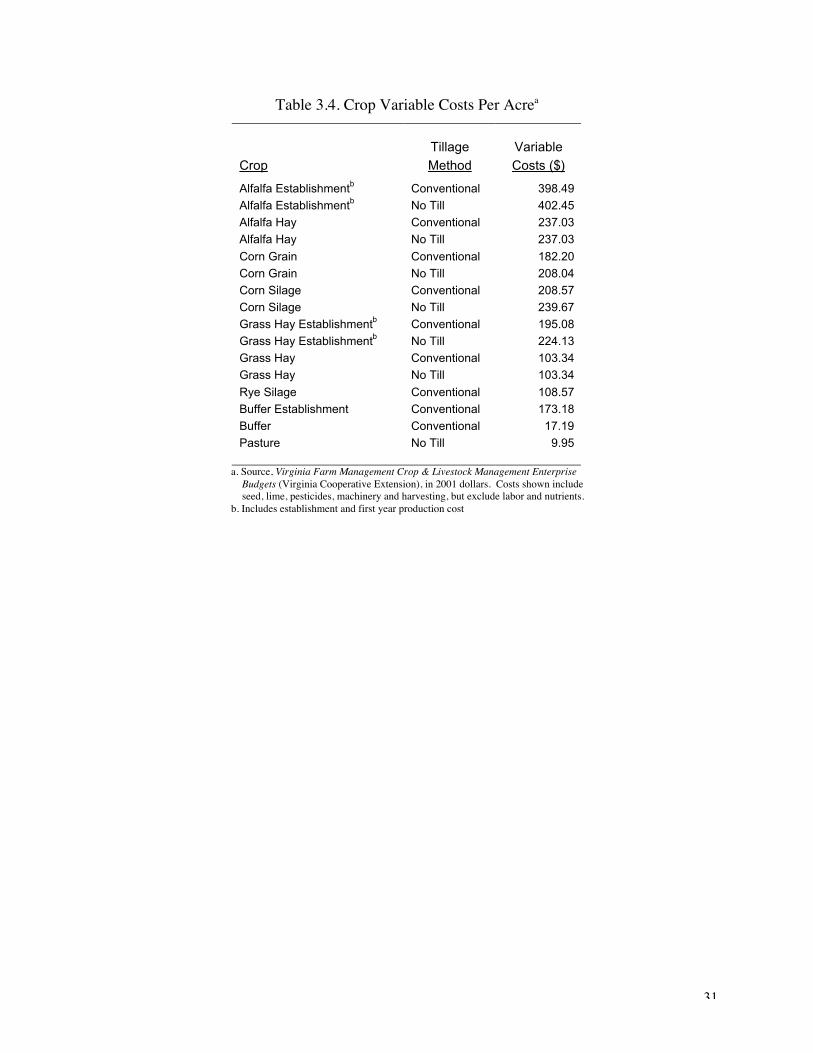
31
Table 3.4. Crop Variable Costs Per Acrea
Tillage Variable
Crop Method Costs ($)
Alfalfa Establishmentb Conventional 398.49
Alfalfa Establishmentb No Till 402.45
Alfalfa Hay Conventional 237.03
Alfalfa Hay No Till 237.03
Corn Grain Conventional 182.20
Corn Grain No Till 208.04
Corn Silage Conventional 208.57
Corn Silage No Till 239.67
Grass Hay Establishmentb Conventional 195.08
Grass Hay Establishmentb No Till 224.13
Grass Hay Conventional 103.34
Grass Hay No Till 103.34
Rye Silage Conventional 108.57
Buffer Establishment Conventional 173.18
Buffer Conventional 17.19
Pasture No Till 9.95
a. Source, Virginia Farm Management Crop & Livestock Management Enterprise Budgets (Virginia Cooperative Extension), in 2001 dollars. Costs shown include seed, lime, pesticides, machinery and harvesting, but exclude labor and nutrients.
b. Includes establishment and first year production cost

32
Table 3.5. Crop Labor Requirements: Hours Per Acrea
CropTillageMethod Spring Summer Fall Total
Alfalfa Establishment Conventional 2.77 1.34 0.67 4.78
Alfalfa Establishment No Till 1.22 1.34 0.67 3.23
Alfalfa Hay Conventional 0.67 1.34 0.67 2.68
Alfalfa Hay No Till 0.67 1.34 0.67 2.68
Corn Grain Conventional 1.41 0.00 0.00 1.41
Corn Grain No Till 0.50 0.00 0.00 0.50
Corn Silage Conventional 1.22 0.00 0.93 2.15
Corn Silage No Till 0.50 0.00 0.93 1.43
Grass Hay Establishment Conventional 1.89 1.00 0.00 2.89
Grass Hay Establishment No Till 0.55 1.00 0.00 1.55
Grass Hay Conventional 0.20 1.00 0.00 1.20
Grass Hay No Till 0.20 1.00 0.00 1.20
Rye Silage Conventional 0.93 0.00 0.88 1.81
Buffer Establishment Conventional 0.00 0.00 0.00 0.00
Buffer Conventional 0.00 0.00 0.00 0.00
Pasture No Till 0.20 0.53 0.00 0.73
a. Source, Virginia Farm Management Crop & Livestock Management Enterprise Budgets (Virginia Cooperative Extension) b. Buffer establishment and maintenance are done with custom-hired machines.
Nitrogen, phosphate (P2O5), and potash (K2O) are nutrients available for use in crop
production. Nutrient sources include dairy manure, poultry litter, and commercial
fertilizers—ammonium nitrate (33% N), triple super phosphate (46% P2O5), and muriate of
potash (60% K2O). Purchase prices and application costs of the nutrient sources are shown in
Table 3.6. Manure and litter can be applied at all times of the year; commercial nitrate can be
applied during the spring, summer and fall; and commercial phosphate and potash can be applied
during spring and fall. Other restrictions exist on specific crops, for example: rye silage can only
receive manure and poultry litter in the fall and winter; commercial phosphate and potash in fall;
and commercial nitrate in fall and spring. Minimum recommended nutrient applications were
taken from VALUES (Donohue et al.). Recommended N for corn grain is 1 lb./bu. The
recommendation for corn silage is 7.5 lbs./ton, which is based on a yield range of 10–21 tons.
The recommendation for grass hay is 40 lbs./acre during establishment and 0 lbs./acre during
maintenance. Recommended applications of N are 22 lbs./ton of rye silage for all soil classes
and 0 lbs. for alfalfa and pastures.
Normally a soil test would be performed to determine P and K recommendations.
However, soil test information available for Rockingham County could not be tied to specific
farms. Therefore, a method was developed to estimate P and K levels based on farm dairy and

33
poultry production (Pease). Cow-calf and stocker manure production was not included because
these enterprises are produced on pasture and the manure is not recovered. The method consists
of dividing the total manure/litter phosphate and potash production of the farm by the total acres
of crop fields. If potential nutrients (lbs.) per acre are 0–120 then the soil tests for both P and K
are medium; if 120–180 then high; and if greater than 180 then very high. Recommended levels
of phosphate and potash based on the soil test estimates are shown in Table 3.7. Phosphate
removal per unit of crop yield is 0.4 lbs/bu. for corn grain, 7.5 lbs./ton for corn silage, 5.6
lbs./ton for rye silage, 11 lbs./ton for alfalfa; and 15 lbs./ton for grass hay and pastures
(Chesapeake Bay Region Nutrient Management Training Manual). Phosphate removal per acre
of crop (lbs.), which is used in the application of nutrient management plans, is found at the field
level by multiplying the yield of each crop for the field by the corresponding removal rate.
Recommendations for applications of each nutrient are found for each crop-fieldcombination by multiplying the minimum recommendations discussed above multiplied by the
field yield potentials. FARMPLAN selects the level of each nutrient source spread over eachcrop-tillage-field-season combination. Nutrients spread for each crop-tillage-field combination
over all seasons must be greater than or equal to the recommended nutrient level for each crop-
tillage-field combination. Summing the levels of nutrients spread over crops, tillage and fieldsprovides total nutrients spread for the farm. Levels of nutrient sources spread are also summed
over crops, tillage and fields to derive the total quantity of each nutrient source spread on the
farm during each season. Nutrient sources spread in a season are limited to the quantities boughtand produced—in the case of farm manure—in the same season. Manure produced in previous
seasons can be spread if adequate storage is available to carry the manure to the desiredspreading season. Phosphorous applications and removal are calculated at the field and farm
levels. Application costs and the costs of nutrients purchased are calculated at the farm level.

34
Table 3.6. Nutrient Purchase and Application Costsa by Source and Season
Purchase Costs ($) Application
Nutrient Source Spring Summer Fall Winter Costs ($)b
Dairy Manure (1,000 gal.) 5.00 5.00 5.00 5.00 7.37Broiler Litter (ton) 14.00 10.00 12.00 10.00 5.24Turkey Litter (ton) 12.50 9.00 10.50 9.00 5.24
Commercial Ammonium Nitrate (cwtc) 9.00 9.00 9.00 9.00 0.98Commercial Triple Super Phosphate (cwt) 11.04 11.04 11.04 11.04 0.98Commercial Muriate of Potash (cwt) 9.00 9.00 9.00 9.00 0.98
a. Source, Virginia Farm Management Crop & Livestock Management Enterprise Budgets (Virginia Cooperative Extension), 2001 dollars b. Includes hauling and application costs c. Hundred weight
Table 3.7. Crop Nutrient Recommendationsa
Phosphate [P2O5] Potash [K2O]
Crop / Soil Test Range Medium HighVeryHigh Medium High
VeryHigh
Lbs. Per Unit of Crop
Corn Grain [bu]b 0.5 0.3 0.0 0.5 0.3 0.0
Corn Silage [ton]c 4.0 2.0 0.0 8.0 4.0 0.0
Rye Silage [ton]d 20.0 10.0 0.0 20.0 10.0 0.0
Alfalfa Establishment [acre]e 130.0 80.0 0.0 130.0 80.0 0.0
Alfalfa [ton]f 12.5 8.0 0.0 38.0 19.0 0.0
Grass Hay Establishment [acre]g 130.0 75.0 0.0 130.0 75.0 0.0
Grass Hay [ton]h 20.0 12.5 0.0 42.5 22.5 0.0
Pasture [grass hay equivalent]h 20.0 12.5 0.0 40.0 22.5 0.0
Buffer Establishment [acre]g 130.0 75.0 0.0 130.0 75.0 0.0
Buffer [acre]g 50.0 50.0 0.0 50.0 55.0 0.0
a. Source, VALUES (Donohue et al.) b. Based on 65–165 bushels c. Based on 10–21 tons d. Based on 2–4.5 tons e. All soils f. Based on 3.5–6.5 tons g. Assumed red-clover orchard grass mix h. Based on 2.5–4 tons
FARMPLAN selects the level (acres) of each crop rotation for each field on the farm.
The levels of each rotation are summed and the total must be less than or equal to the size of thefield. The level (acres) of each crop-tillage combination on a field is determined by multiplying
the crop weight within the rotation by the corresponding rotation level, then summing over the
rotations. Then the levels (acres) of each crop are summed over the tillage methods to determinethe total level of each crop type for a field. The total yield of each crop product produced on the
farm is then found by multiplying crop acreage by the corresponding yield and summing over all

35
fields and tillage types. Crop products can be either sold or used as feed. Each crop product is
balanced so that the sum of products sold and products fed to livestock equals the sum ofproducts purchased and products produced. Crop revenue is calculated at the crop level for each
farm and then summed over the set of crops. Variable costs for the crops are calculated bymultiplying total acres of each crop-tillage combination for the farm by the corresponding cost
rate and then summing over tillage and crops. Similarly, crop labor use is calculated by
multiplying total acres of each crop-tillage combination for the farm by the corresponding laborrequirement and then summing over tillage and crops.
3.3.2 Livestock and Manure
Livestock include dairy cows, beef cows, beef stockers, chicken broilers, and turkeys.Dairy cows are dry for 60 days of the year and lactate the remaining 305. A stocker steer is kept
from early March to fall and weighs 450 lbs. at purchase and 715 lbs. at sale. A stocker requires
half the capacity of a beef cow, i.e. a farm that can accommodate 50 beef cows can accommodate100 stockers. A herd of beef cows includes 1 bull for every 25 cows and each cow produces 1
calf, of which 90% survive. The offspring consist equally of heifers and bulls; all of the bullsand two-thirds of the heifers are sold and the remaining heifers are kept to replace the 1% of
cows lost to death and the culling of 14% of the herd. One bull is bought and one bull is culled
each year.A single broiler house runs 6.4 cycles of 25,000 birds in a year and a turkey house runs 4
cycles of 16,000 birds (Virginia Dept. of Conservation and Recreation). An integrator providesthe birds, rations, management advice, and markets the finished birds. The farmer provides the
labor, housing and energy, and receives a commission per bird paid by the integrator.
The set of livestock products for sale includes milk, beef stockers, weaned beef calves,chicken broilers, and turkeys. Annual livestock yields and selling prices are shown in Table 3.8,
which shows the type of livestock, the product sold, the product units, the level of units yielded
(per cow for dairy and beef, and per house for poultry), and the selling price per unit of product.For example, a dairy cow yields 180 cwt of milk annually which is sold at $14.00 per cwt. Dairy
and beef cow activities also get income from herd culls. Cull income was prorated overproducing cows. The result is that for each dairy cow $145.60 is earned as income from culls,
and for each beef cow $64.00 is earned. Dairy income is also earned from bull calf sales
($35.63/cow) and patronage refunds ($126/cow).

36
Variable costs are shown in Table 3.9 and include expenses for minerals, veterinarian and
medical services, replacement units, supplies, building and fence repair, machinery, and utilities;complete budgets are provided in Appendix B. Feed and labor expenses are excluded and
determined separately. Labor requirements by livestock type and season are also shown in Table3.9. All of the crops produced on the farm are available for feed, and as mentioned in the crop
and nutrients section above, corn, alfalfa and grass hay can also be bought. Soybean oil meal can
be purchased for $225 per ton. Dairy cows also require mineral supplements, which includedicalcium phosphate, limestone and a combination of other minerals that can be purchased for
$219, $23 and $400 per ton, respectively. Dairy cows are given one of three feed rations, shownin Table 3.10, that are comprised of various quantities of crop products, soybean oil meal, and
supplementary minerals. Beef stockers and cows are given rations of corn grain and grass hay,
shown in Table 3.10. Poultry rations are supplied by poultry integrators and are not included inthe enterprise budgets used to determine variable costs. Feed costs are indexed over the set of
crop products and are calculated only for feed purchased. The cost of feed grown on the farm is
not measured as part of feed costs, its cost is included with the cost of crop production measuredin the crop and nutrient section.
The set of recoverable manure includes dairy manure, broiler litter and turkey litter. Beefcow and stocker manure is not recoverable. A lactating dairy cow produces 14,230 gallons of
recoverable manure a year, which includes feedlot runoff, dairy wash water, and runoff into the
manure storage facility. Chicken broiler and turkey houses produce 200 tons and 640 tons oflitter per year, respectively. These figures, along with the corresponding nutrient content, are
summarized in Table 3.11. Recoverable manure can be used as a nutrient source for crops,stored or sold. Dairy manure for sale has a market range of 60 miles from the source farm.
Selling prices vary by season and are shown in Table 3.12. Manure storage capacity is measured
in months and is indexed over the set of recoverable manure. Dairy and poultry farms areassumed to have six months storage capacity, which is common for farms in the area (Spitler).
In terms of manure quantity, capacity is derived by multiplying months of capacity timeslivestock capacity times monthly manure production per unit (i.e. cow or house). For example, a
farm with 100 dairy cows and six months of storage will have 711,500 gallons of storage
capacity (6 * 100 * 14,230 ÷ 12). Manure storage allows farms to hold the manure from seasonswhen the farm produces a surplus of nutrients—crop nutrient requirements are lower than

37
nutrients produced—and spread it in seasons when crop and soil conditions are right for manure
spreading. Annual recoverable manure is allocated over seasons equally by dividing the quantityproduced by four.
Table 3.8. Annual Livestock Yields and Selling Pricesa
Selling
Livestock Product Unitsb Yield Price ($)Dairy Cow Milk cwt 180.00 14.00
Beef Stocker Stocker cwt 7.15 85.00
Beef Cow Weaned Calf cwt 4.25 88.48
Broiler Broiler 1,000 birds 160.00 166.41c
Turkey Turkey 1,000 birds 64.00 1,099.15c
a. Source, Virginia Farm Management Crop & Livestock Management Enterprise
Budgets (Virginia Cooperative Extension), 2001 dollars. b. Per animal for dairy cows, beef stockers and beef cows; and per house for broilers and turkeys c. Commissions received by the farm from poultry integrators for raising birds
Table 3.9. Livestock Variable Costs and Labor Requirementsa
Variable Labor, Hours Required per Livestock Unit
Livestock Units Costs ($) Spring Summer Fall WinterDairy Cowb animal 840.28 15.63 15.63 15.63 15.63
Beef Stockerc animal 565.74 0.23 0.23 0.23 0.00
Beef Cowd animal 81.34 2.00 2.00 2.00 2.00
Broilere house 7,609.00 182.50 182.50 182.50 182.50
Turkeye house 18,630.00 311.47 311.47 311.47 311.47
a. Source, Virginia Farm Management Crop & Livestock Management Enterprise Budgets (Virginia Cooperative Extension), 2001 dollars b. Includes: minerals, milk replacement, calf grower, breeding, veterinary, supplies, milk haul and market for culls, building and fence
repair, machinery, utilities, and custom hire. Excludes: feed, labor, farm insurance, rent and taxes. c. Includes: steer purchase costs, interest, procurement, minerals, veterinary, supplies, haul and market of calves, building and fence repair,
machinery, and utilities. Excludes: feed, labor, farm insurance, rent, and taxes. d. Includes: salts and minerals, veterinary, supplies, replacement bulls, haul and market culls, building and fence repair, machinery, and
utilities. Excludes feed,labor, farm insurance, rent, and taxes. e. Includes: repairs and maintenance, electricity, fuel, bedding material, loader, and scraper. Excludes: labor, feed insurance, rent, and taxes.

38
Table 3.10. Livestock Feed Rations With Crop Products in Tons Per Year
Dairya,b
AlfalfaCorn
SilageRye
Silage Stockerc Beef Cowc
Alfalfa Hay (tons) 4.27 0.76 0.76 0.00 0.00Corn Grain (bu) 143.53 99.96 127.19 2.77 3.50Corn Silage (tons) 0.00 9.91 0.00 0.00 0.00Rye Silage (tons) 0.00 0.00 8.69 0.00 0.00Soybean Oil Meal (tons)d
0.04 0.80 0.39 0.00 0.00Grass Hay (tons)d
5.04 5.04 5.04 1.14 4.93Dical (tons)d
0.07 0.07 0.05Limestone (tons)d
0.00 0.08 0.09Other Minerals (tons)d
0.14 0.14 0.14
a. Source, Knowlton b. Includes dry cow feed and cow’s share of replacement heifer c. Source, Virginia Farm Management Crop & Livestock Management Enterprise Budgets (Virginia Cooperative Extension) d. Included in set of crop products for programming convenience

39
Table 3.11. Manure Nutrient [lbs.] Content
Npe
r un
it of
Live
stoc
k
368
14,3
22
45,9
02
Npe
r un
it of
Man
ure
25.9
0
71.6
1
71.6
1
K2O
per
unit
ofLi
vest
ock
247
8,68
0
27,8
19
K2O
per
unit
ofM
anur
e
17.3
7
43.4
0
43.4
0
P2O
5
per
unit
ofLi
vest
ock
154
11,6
34
37,2
87
P2O
5
per
unit
ofM
anur
e
10.8
4
58.1
7
58.1
7
Uni
ts
1000
gal
.
tons
tons
Ann
ual
Rec
over
able
Man
ure
14.2
3
200.
00
641.
00
Uni
ts
Cow
Hou
se
Hou
se
Tabl
e 3.
11. M
anur
e N
utrie
nt [l
bs.]
Cont
ent
Live
stoc
k
Dai
ry
Bro
ilers
Tur
keys
Sou
rce:
199
8-19
99 te
st v
alue
s re
port
ed in
J. P
ease
and
G. M
ullin
s. "
Virg
inia
Man
ure
Tes
t Sum
mar
ies.
"F
arm
Bus
ines
s M
anag
emen
t Upd
ate ,
Bla
cksb
urg,
VA
: Virg
inia
Pol
ytec
hnic
Inst
itute
and
Sta
te U
nive
rsity
,V
irgin
ia C
oope
rativ
e E
xten
sion
.

40
Table 3.12. Manure Selling Prices By Seasona
Spring Summer Fall Winter
Dairy Manurea-$26.40 -$26.40 -$26.40 -$26.40
Broiler Litterb$8.00 $4.00 $6.00 $4.00
Turkey Litterb$6.50 $3.00 $4.50 $3.00
a. Based on assumption that the farmer pays hauling costs, which are assumed
to cost $26.40 per 1,000 gallons for a distance up to 60 miles. This haul cost was based on haul costs of turkey litter ($0.11/ton mile, Pelletier et al.) and approximately 4 tons per 1,000 gallons. In 2001 dollars.
b. J. Pease 2001, personal communication
Livestock production levels are indexed over livestock and ration types, e.g. dairy cow
and dairy alfalfa ration, or beef cow and beef cow ration. Broiler and turkey rations were not
quantified because all feed is supplied by the integrator. Livestock feed consumption is summed
over ration types to get totals for each livestock type. Feed consumption must be less than or
equal to feed produced and/or purchased by the farm. For example, for every dairy cow raised on
the alfalfa ration, alfalfa hay fed must equal 4.27 tons. Purchased-feed costs equal the level of
feed purchased times the corresponding price. Livestock products are set equal to the quantity of
each livestock type—summed over ration type—times the corresponding yield rate. It is
assumed that all products are sold, therefore products sold equal products produced. Revenue
from livestock products equals the level of products sold times price, and total revenue from
livestock equals the sum of product revenue and income from culls. The variable cost rate of
each livestock type is multiplied by the level of each type. These figures are first summed over
ration type and then livestock type to determine total variable costs by livestock type and farm,
respectively. Labor requirements per livestock unit are annualized—sum of seasonal
requirements—and multiplied by the corresponding level of livestock production, then summed
over livestock and ration types to determine the total annual labor requirement for livestock
activities, which is then used to determine the total annual hours of labor available on the farm.
Seasonal manure levels are calculated by multiplying the seasonal production rate by the
corresponding level of livestock—summed over ration type. Manure produced is convertedeither to crop nutrients, manure for sale, or manure stored. The quantity of manure stored in a
season must be less-than or equal-to storage capacity. Manure produced in a season plus manure
stored the prior season must equal the sum of manure used as crop fertilizer, manure sold, andmanure stored for the current season. For example, spring manure produced plus winter manure
stored must equal the sum of spring manure sales, spring manure used as crop fertilizer, and

41
spring manure stored. Seasonal manure sales are multiplied by the corresponding sale price and
aggregated to determine annual manure revenue.
3.3.3 Best Management Practices
The nutrient management plan limits applications of P from manure and commercial
fertilizer on each field to the crop P removal rate. If manure applications cannot meet all N andK requirements, commercial N and K applications are required. If manure production cannot be
used on farm at these application rates, excess manure must be sold off farm. Nutrient
management plans cost $15 per acre, which includes initial writing costs, soil tests, andmaintenance costs, and have a life of three years (Patterson). Using an interest rate of 5.7%
(Yanosek) the annual cost of a nutrient management plan is $5.58 per acre (NRCS). Buffers are a mixture of bluestem, switch grass and partridge peas. The buffer practice
consists of placing a 100 ft. herbaceous buffer strip on all the border of fields that are adjacent to
receiving waters. The acreage of each field that would fall into the buffer zone was determinedprior to running FARMPLAN and included in the input data. When the buffer policy is
implemented, FARMPLAN requires the farm to put the designated acreage of each field into thebuffer rotation. The total cost per acre to establish a buffer is $173.18. After the buffer has been
established, costs of $17.85 per acre per year are required to maintain it. With a life of ten years
the average annual cost of an acre of buffer is $32.79. The buffer is assumed to not be harvested.
3.4 Phosphorous Delivery Model
As described in section 2.4, PDM (Veith; Mullins et al. 2002b) was constructed in ESRIArcView GIS, the program is provided in Appendix C. The total quantity of P delivered (lbs.)
(TP) to the watershed outlet from each field is given by the sum of sediment-P (SP) and runoff-P
(RP):
TP = SP + RP (3.1)
The foundation of PDM is the sediment and runoff routing functions with P-concentration
coefficients determining the quantity of P that is delivered with the sediment and runoff. PDM
was programmed so that each component can be estimated at the cell, field, farm, and watershedlevels. Cells are 30-meters square.

42
3.4.1 Sediment-P
Gross erosion (A) is estimated using the USLE, equation 2.7. The R factor is a constant
of 2800 SI (Schwab et al.); the K factor (USDA, 2001) is contained in a GIS data layer; slopelength (l), used to calculate the L factor, is a constant 45 meters; and slope steepness (s), used to
calculate both the L and S factors, comes from the digital elevation model that is part of the base
data set. The C factors, shown in Table 3.13, were provided by a representative of the U.S. FarmService Agency in Rockingham County, VA. The P factor is a constant of 1 because no
applicable conservation practices are used—contouring, terracing or strip cropping. The
sediment delivery ratio (d) of each cell is calculated using equation 2.8 and the land usecoefficients (alpha(a)) (Veith) shown in Table 3.13. The slope and flow length factors are
determined by the GIS using the digital elevation model and land use data layer. Using gross
erosion from the USLE, and the sediment delivery ratio, the sediment routing function (equation2.6) calculates the sediment yield (Y) from each cell to the watershed outlet. A distribution of
Mehlich I soil test values for Rockingham County3, shown in Table 3.14, were provided by
Mullins et al. (2002a) and used to calculate the sediment-P coefficients (rho(r)) (equation 2.9).
The Mehlich I test values from the Mullins study were randomly assigned to the fields.Sediment-P (SP) as shown in equation 2.3 is the product of sediment yield and the sediment-P
coefficient.
3 FARMPLAN assumes soil P values are livestock dependent, whereas PDM assumes they are random. TheMehlich I test values were provided as a distribution and were therefore not applicable to FARMPLAN.

43
Table 3.13. Land Use Factors of Crop Rotations for Calculating Deliveriesa
Crop Rotation C Factorb Alphac Betad
NTCG 0.01 4.9 9.8
CTCG 0.18 9.7 19.4
NTCS 0.16 4.9 9.8
CTCS 0.32 9.7 19.4
NTCGRYE 0.04 3.1 6.2
CTCGRYE 0.18 6.2 12.4
NTCSRYE 0.15 3.1 6.2
CTCSRYE 0.21 6.2 12.4
NTCGALF 0.08 3.8 15.7
CTCGALF 0.14 5.1 5.3
NTCSALF 0.06 3.8 15.7
CTCSALF 0.09 5.1 5.3
CTGRHAY 0.02 3.3 6.6
NTGRHAY 0.01 3.3 6.6
PERMPAST 0.01 1.6 3.2
BUFFER 0.01 1.6 3.2 a. Phosphorous Delivery Model
b. Land use coefficient used in the USLE c. Land use coefficient used to calculate the sediment delivery factor (d) d. Land use coefficient used to calculate the runoff delivery factor (b)
Table 3.14. Mehlich I Soil Test Distributiona
Category DistributionP
[lbs./a]
Low 6.7% < 12
Medium 22.3% 12 - 35
High 39.1% 36 - 110
Very High 31.9% > 110
a. Source, The Virginia Phosphorous Index: A Planning Tool for Phosphorous Management. Mullins et al 2002a.
3.4.2 Runoff-P
Average annual runoff (RO) is found using national climatic data, which is grouped into
geographic zones, and the curve number method. The majority soil present in each cell was usedto determine the hydrologic soil group (USDA, 2001). The land use description is determined by
the FARMPLAN selected crop rotation. The hydrologic soil group is cross-referenced with theland use description to find the corresponding curve number (U.S. Soil Conservation Service).
The curve number is then cross referenced with the climatic zone—Rockingham County is in the
Central Mountain Division 5—to identify the appropriate level of average annual runoff. Therunoff delivery ratio (b) is specified using equation 2.11 and the land use coefficients (beta(_))

44
(Veith) shown in Table 3.13. The runoff routing function (equation 2.10) calculates runoff yield
(ROY) from average annual runoff, cell area and the delivery ratio. The Mehlich I soil testvalues are used in equation 2.12 to determine the runoff-P coefficient (sigma(s)). The fertilizer
source availability factor for manure/litter is 0.2. It was assumed that the manure is surface
applied with no incorporation, which has a factor of 0.2. The product of the two factorsdetermines the applied fertilizer factor (APF), 0.04. Equation 2.4 is used to calculate runoff-P
(RP), which is the product of runoff yield and the runoff-P coefficient plus the product of
applied-P and the applied fertilizer factor.A requirement of the GIS version of PDM is that the farms and fields of interest have to
represent real geographic points. As described below, the representative and typical farms are
hypothetical, and although the mega farm represents the entire watershed, the specific locationsof its fields are unknown because soil resources were aggregated. Most of the P delivery
calculations can be made by hand, in a spreadsheet or in the GAMS compiler. The limitationsare the K, L and S factors, and the d (sediment delivery ratio) and b (runoff delivery ratio)
components since they require the elevation map found in the GIS. To determine these factors
for the alternative information cases, PDM was run for the population under each policyscenario. The R,K,L, and S factors were combined as one factor, RKLS, for each cell. The
RKLS factor for each field was then determined by:
J
RKLSRKLS j
iÂ=
)()( (3.2)
where j represents a cell in field i and J is the total number of cells in field i. The sediment
delivery ratio across a cell is designated as dj, and the delivery ratio from a cell to the outlet isdesignated as Dj and is determined by:
’=
=K
jkkj dD (3.3)
where k represents a cell in the flow path of cell j—the source cell is included in the flow path.The sediment delivery ratio for each field was therefore calculated as:
J
D
D
J
jj
i
Â== 1 (3.4)

45
or the average of the cell delivery ratios. The same process is followed for the runoff delivery
ratios:
’=
=K
jkkj bB (3.5)
and
J
B
B
J
jj
i
Â= (3.6)
With approximations of the RKLS, d, and b components for each field in the population,PDM was reconstructed in GAMS, using the approximations as input parameters. The
approximations were assigned to the hypothetical fields in the three alternative cases, which are
described in detail below.
3.5 Information Cases
3.5.1 Population
Using the data cited in section 3.2, Conrad Heatwole of Virginia Tech supervised the firststage of the process that defined the population of farms in the Muddy Creek Watershed. An
agent for the Virginia Department of Conservation and Recreation used the photographs to
determine field boundaries for the land use data layer. Expert opinion was then used todetermine an initial distribution of farm types, farm enterprise information, and animal
production feed requirements for the area (Schroeder; Virginia Department of Environmental
Quality; Parsons; US-Department of Commerce). Approximately 120 farm generation pointswere selected within and surrounding the watershed boundaries. Farm points were determined
from the set of farmsteads and poultry houses designated in the land use coverage, while pointsoutside the watershed were randomly determined. All farm generation points were randomly
assigned farm types from the following distribution: 65% dairies, 30% beef cattle, and 5%
poultry. All farm points that started from a poultry house were designated as poultry, or dairy orbeef with poultry. The distribution of farm types was based on a summary (Pease) of expert
opinion (Schroeder, Parsons, and Virginia Department of Environmental Quality).The Thiessen Polygon method was used to assign land to the closest farm point. The
farm-point data layer was then converted into a polygon layer. The polygon matrix was draped
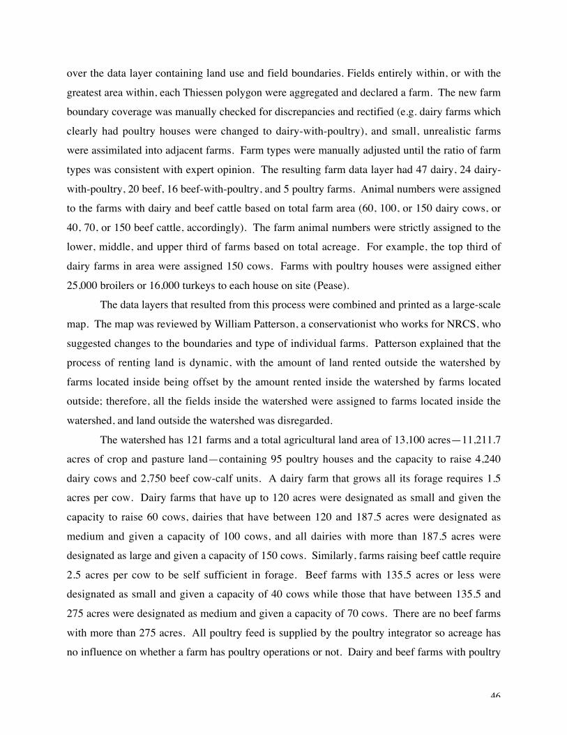
46
over the data layer containing land use and field boundaries. Fields entirely within, or with the
greatest area within, each Thiessen polygon were aggregated and declared a farm. The new farmboundary coverage was manually checked for discrepancies and rectified (e.g. dairy farms which
clearly had poultry houses were changed to dairy-with-poultry), and small, unrealistic farmswere assimilated into adjacent farms. Farm types were manually adjusted until the ratio of farm
types was consistent with expert opinion. The resulting farm data layer had 47 dairy, 24 dairy-
with-poultry, 20 beef, 16 beef-with-poultry, and 5 poultry farms. Animal numbers were assignedto the farms with dairy and beef cattle based on total farm area (60, 100, or 150 dairy cows, or
40, 70, or 150 beef cattle, accordingly). The farm animal numbers were strictly assigned to thelower, middle, and upper third of farms based on total acreage. For example, the top third of
dairy farms in area were assigned 150 cows. Farms with poultry houses were assigned either
25,000 broilers or 16,000 turkeys to each house on site (Pease).The data layers that resulted from this process were combined and printed as a large-scale
map. The map was reviewed by William Patterson, a conservationist who works for NRCS, who
suggested changes to the boundaries and type of individual farms. Patterson explained that theprocess of renting land is dynamic, with the amount of land rented outside the watershed by
farms located inside being offset by the amount rented inside the watershed by farms locatedoutside; therefore, all the fields inside the watershed were assigned to farms located inside the
watershed, and land outside the watershed was disregarded.
The watershed has 121 farms and a total agricultural land area of 13,100 acres—11,211.7acres of crop and pasture land—containing 95 poultry houses and the capacity to raise 4,240
dairy cows and 2,750 beef cow-calf units. A dairy farm that grows all its forage requires 1.5acres per cow. Dairy farms that have up to 120 acres were designated as small and given the
capacity to raise 60 cows, dairies that have between 120 and 187.5 acres were designated as
medium and given a capacity of 100 cows, and all dairies with more than 187.5 acres weredesignated as large and given a capacity of 150 cows. Similarly, farms raising beef cattle require
2.5 acres per cow to be self sufficient in forage. Beef farms with 135.5 acres or less weredesignated as small and given a capacity of 40 cows while those that have between 135.5 and
275 acres were designated as medium and given a capacity of 70 cows. There are no beef farms
with more than 275 acres. All poultry feed is supplied by the poultry integrator so acreage hasno influence on whether a farm has poultry operations or not. Dairy and beef farms with poultry

47
operations have an average of 2 poultry houses while poultry farms have 3 houses.
Approximately 57% of poultry operations raise turkeys and the remainder raise broilers. Thereis no correlation between poultry type and other livestock; however, to minimize the number of
farm types all dairy-with-poultry farms were described as raising broilers and all beef-with-poultry farms were described as raising turkeys.
Tables 3.15 through 3.17 summarize the population of farms. Table 3.15 shows the
number of farms of each type, and the total livestock numbers of the member farms. Table 3.16shows the total number of fields of the farms for each type, the combined acreage of the fields,
and the average per acre crop yields. Table 3.17 shows the average values of the factors used inPDM, and the total number of acres that would be forced into buffers under that policy. The
averages were weighted by field size, except the buffers which were summed over all the fields.
The number of potential buffer acres for each field was determined using tools in theGIS. Fields were identified as either being adjacent to a stream or not, and the acres of buffer
resulting from a 30 meter (100 ft) filter strip were calculated. A total of 1,187.7 acres of
potential buffer area exist in the watershed. Mehlich I soil test values were randomly assigned tofields based on the distribution from Mullins et al. (2002a) to be used in PDM. A complete
description of each farm can be found in Appendix D.In summary, the data are indexed over farms and fields and contain: farm type; livestock
capacity; field size; crop yields; the sediment-P and runoff-P coefficients derived from the
Mehlich I soil test values; potential buffer acres; and the sediment and runoff delivery ratioscalculated using PDM.

48
Table 3.15. Distribution of Farms in Muddy Creek Watershed With Livestock Capacities
Farm Type# of
FarmsDairyCows
BeefCows
BroilerHouses
TurkeyHouses
Small Dairy 27 1,620 0 0 0
Medium Dairy 9 900 0 0 0Large Dairy 3 450 0 0 0Small Dairy-with-Broilers 12 720 0 24 0Medium Dairy-with-Broilers 4 400 0 8 0Large Dairy-with-Broilers 1 150 0 2 0
Small Beef 31 0 1,240 0 0Medium Beef 5 0 350 0 0Small Beef-with-Turkeys 22 0 880 0 44Medium Beef-with-Turkeys 4 0 280 0 8Broiler Only 2 0 0 6 0Turkey Only 1 0 0 0 3
Total 121 4,240 2,750 40 55
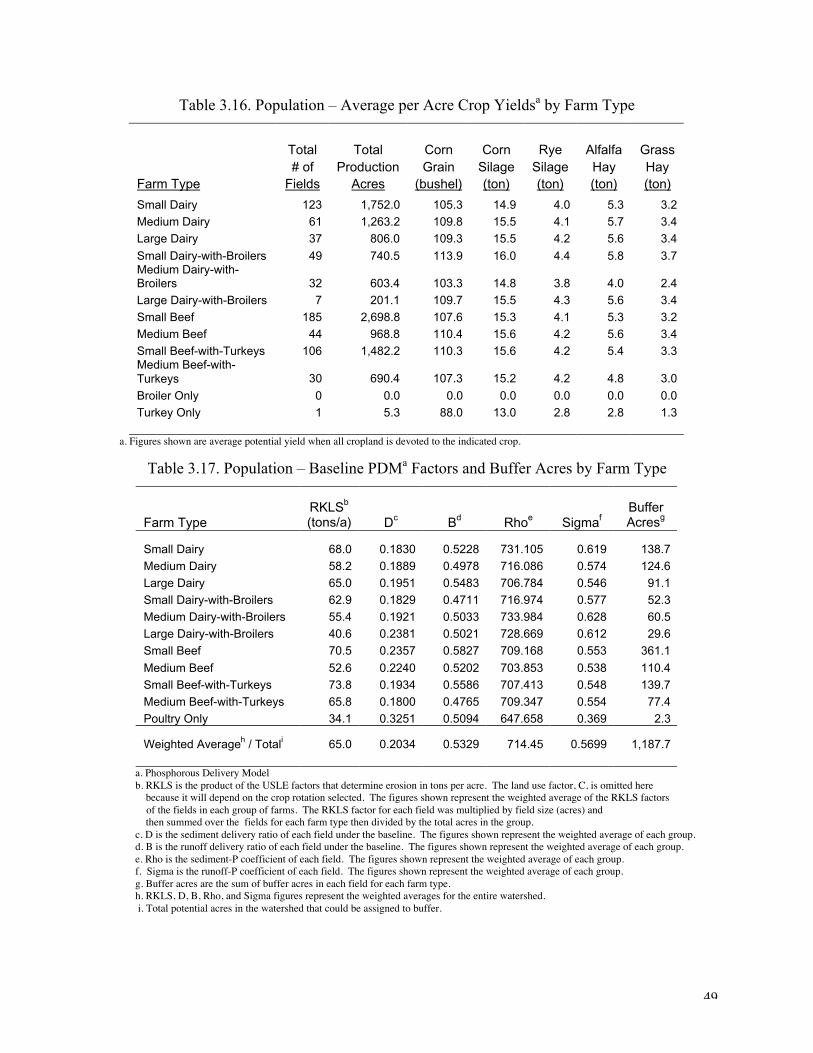
49
Table 3.16. Population – Average per Acre Crop Yieldsa by Farm Type
Total Total Corn Corn Rye Alfalfa Grass# of Production Grain Silage Silage Hay Hay
Farm Type Fields Acres (bushel) (ton) (ton) (ton) (ton)
Small Dairy 123 1,752.0 105.3 14.9 4.0 5.3 3.2
Medium Dairy 61 1,263.2 109.8 15.5 4.1 5.7 3.4
Large Dairy 37 806.0 109.3 15.5 4.2 5.6 3.4
Small Dairy-with-Broilers 49 740.5 113.9 16.0 4.4 5.8 3.7Medium Dairy-with-Broilers 32 603.4 103.3 14.8 3.8 4.0 2.4
Large Dairy-with-Broilers 7 201.1 109.7 15.5 4.3 5.6 3.4
Small Beef 185 2,698.8 107.6 15.3 4.1 5.3 3.2
Medium Beef 44 968.8 110.4 15.6 4.2 5.6 3.4
Small Beef-with-Turkeys 106 1,482.2 110.3 15.6 4.2 5.4 3.3Medium Beef-with-Turkeys 30 690.4 107.3 15.2 4.2 4.8 3.0
Broiler Only 0 0.0 0.0 0.0 0.0 0.0 0.0
Turkey Only 1 5.3 88.0 13.0 2.8 2.8 1.3
a. Figures shown are average potential yield when all cropland is devoted to the indicated crop.
Table 3.17. Population – Baseline PDMa Factors and Buffer Acres by Farm Type
Farm TypeRKLSb
(tons/a) Dc Bd Rhoe SigmafBufferAcresg
Small Dairy 68.0 0.1830 0.5228 731.105 0.619 138.7
Medium Dairy 58.2 0.1889 0.4978 716.086 0.574 124.6
Large Dairy 65.0 0.1951 0.5483 706.784 0.546 91.1
Small Dairy-with-Broilers 62.9 0.1829 0.4711 716.974 0.577 52.3
Medium Dairy-with-Broilers 55.4 0.1921 0.5033 733.984 0.628 60.5
Large Dairy-with-Broilers 40.6 0.2381 0.5021 728.669 0.612 29.6
Small Beef 70.5 0.2357 0.5827 709.168 0.553 361.1
Medium Beef 52.6 0.2240 0.5202 703.853 0.538 110.4
Small Beef-with-Turkeys 73.8 0.1934 0.5586 707.413 0.548 139.7
Medium Beef-with-Turkeys 65.8 0.1800 0.4765 709.347 0.554 77.4
Poultry Only 34.1 0.3251 0.5094 647.658 0.369 2.3
Weighted Averageh / Totali 65.0 0.2034 0.5329 714.45 0.5699 1,187.7
a. Phosphorous Delivery Model b. RKLS is the product of the USLE factors that determine erosion in tons per acre. The land use factor, C, is omitted here because it will depend on the crop rotation selected. The figures shown represent the weighted average of the RKLS factors
of the fields in each group of farms. The RKLS factor for each field was multiplied by field size (acres) and then summed over the fields for each farm type then divided by the total acres in the group. c. D is the sediment delivery ratio of each field under the baseline. The figures shown represent the weighted average of each group. d. B is the runoff delivery ratio of each field under the baseline. The figures shown represent the weighted average of each group. e. Rho is the sediment-P coefficient of each field. The figures shown represent the weighted average of each group. f. Sigma is the runoff-P coefficient of each field. The figures shown represent the weighted average of each group. g. Buffer acres are the sum of buffer acres in each field for each farm type. h. RKLS, D, B, Rho, and Sigma figures represent the weighted averages for the entire watershed. i. Total potential acres in the watershed that could be assigned to buffer.

50
3.5.2 Representative Farm
In section 2.2 the case of the representative farm is described as one where an analyst has
digital data layers containing the soil inventory, topography, surface waters, field boundaries,and land use patterns. A local expert is used to provide the socioeconomic information: number,
types, and size of farms, and livestock capacity. The representative farm was designated as a
dairy-with-poultry because it is the most important farm type in the watershed in terms ofrevenue, and because of the important environmental implications of spreading dairy and poultry
manure. In order to isolate the effects of aggregation it was assumed that the expert estimated
the “true” number of farms in the watershed, 121. The farm size was determined by dividing thetotal acres of crop land in the watershed by 121. The average number of fields per farm in the
population is six, found by dividing the total number of fields, 675, by the estimated number offarms, 121. The result was a farm with 92.7 acres spread over six fields. Diversity of resources
is not affected by the size of each field; therefore, to simplify the process of assigning parameter
values each field was assigned the same number of acres, 15.45. At 92.7 acres the farm fits thescale of a small dairy-with-poultry and was therefore given the capacity to raise 60 cows and has
one broiler house. Although farms of this type are assumed to have two poultry houses thesecond broiler house was omitted to reduce the bias in aggregation. One poultry house per small
dairy comes closer to the number of poultry houses per 100 acres on dairies in the watershed.
Buffer acres were assigned by dividing the total number of buffer acres in the population by 121.Crop yields, and the pollution factors—RKLS, D, B, _, and _—were weighted by field size and
averaged by dividing the sum of the weighted values by total population acres. Because buffersare a transport interruption practice, their effects will be on the sediment and runoff delivery
ratios. In order to capture the effects of the buffers in PDM it was necessary to use the results of
PDM for the population of fields to estimate values of D and B for the representative farm.Separate D and B values were estimated for the portions of fields remaining in production and
for the portions placed in buffers. Field size, crop yields, and PDM factors are shown in tables3.18 and 3.19.

51
Table 3.18. Representative Farm – Crop Yields
# ofFields
TotalAcres
CornGrain(bu/a)
CornSilage
(tons/a)
RyeSilage
(tons/a)
AlfalfaHay
(tons/a)
GrassHay
(tons/a)
6 92.7 108.4 15.3 4.1 5.3 3.2
Table 3.19 Representative Farm – PDMa Factors and Buffer Acres
RKLSb
(tons/a) Dc Bd Rhoe SigmafBufferAcresg
Cropland Underthe Baseline & NMPScenariosh
65.0 0.1389 0.1704 714.45 0.5699 10.5
Cropland Underthe Buffer Scenarioh 65.0 0.0842 0.1107 714.45 0.5699 10.5
Field Buffersh65.0 0.4864 0.5612 714.45 0.5699 10.5
a. Phosphorous Delivery Model b. RKLS is the product of the USLE factors that determine erosion in tons per acre. The land use factor, C, is omitted here
because it will depend on the crop rotation selected. Figures represent the weighted average of all fields in the watershed. c. D is the sediment delivery ratio of each field under the baseline. The figures shown represent the weighted average of all fields in the watershed. d. B is the runoff delivery ratio of each field under the baseline. The figures shown represent the weighted average of all fields in the watershed. e. Rho is the sediment-P coefficient of each field. The figures shown represent the weighted average of all fields in the
watershed. f. Sigma is the runoff-P coefficient of each field. The figures shown represent the weighted average of all fields in the
watershed. g. Potential area that could be assigned to buffers. h. The population baseline results were used to derive RKLS, D and B for the representative baseline and NMP case scenarios. The population buffer results were used to derive D and B for the fields and buffers for the buffer case. Delivery calculations for cropland include the buffers, the delivery coefficients of the buffers are imbedded in the
delivery coefficients of the crop fields.
3.5.3 Mega Farm
The mega farm represents the watershed as a single farm that contains the watershed’s
entire inventory of cropland and livestock facilities. Recall from section 2.2 that the analyst hasno information on field or farm boundaries, but is provided with an estimate of the total livestock
capacity of the watershed. The farm has 11,211.7 acres of crop and pasture land and the capacity
for 4,240 dairy cows, 2,750 beef cows, 40 broiler houses, and 55 turkey houses. FARMPLANrequires the case to be described in terms of farms and fields, so fields were determined by
grouping the soil inventory by yield with each group forming a mega field. The population datawere organized in a spreadsheet with each of the 675 fields occupying a row and the various
parameters occupying the columns. The rows, or fields, were sorted by crop yields, resulting in

52
23 mega fields, shown in Table 3.20. Each of the PDM factors, which vary by field, was
multiplied by field size. Each of the 23 mega fields was then described by summing the fieldsize of the underlying fields, the relevant crop yields, the weighted average of the PDM factors,
and the sum of the potential buffer acres of the underlying fields. Just as in the representativecase, alternative D and B values were also derived for the buffer scenario. Crop yields and
physical factors for the mega fields are shown in tables 3.20 and 3.21, respectively.
Table 3.20. Mega Farm – Crop Yields
FieldProduction
Acres
CornGrain(bu/a)
CornSilage
(tons/a)
RyeSilage
(tons/a)
AlfalfaHay
(tons/a)
GrassHay
(tons/a)
1 85.3 0.0 0.0 0.0 0.0 1.3
2 66.4 52.0 8.9 2.5 0.0 1.3
3 12.5 55.3 9.3 2.7 0.0 1.3
4 502.8 65.0 10.4 1.5 0.0 1.3
5 81.8 72.3 11.2 4.3 0.0 1.3
6 115.6 85.0 12.7 2.7 0.0 1.3
7 5.9 85.0 12.7 5.0 7.0 5.0
8 112.5 88.0 13.0 2.8 0.0 1.3
9 4.5 88.0 13.0 4.0 2.8 1.3
10 22.8 90.0 13.3 2.8 0.0 1.3
11 85.5 96.8 14.0 4.4 3.1 1.4
12 240.9 100.0 14.4 3.1 0.0 1.3
13 39.7 100.0 14.4 3.8 0.0 1.3
14 2,518.1 104.0 14.9 4.0 5.6 3.4
15 13.6 110.0 15.5 5.0 3.5 1.6
16 9.5 110.5 15.6 4.3 3.0 3.6
17 6,323.2 114.4 16.0 4.4 6.2 3.7
18 23.9 114.4 16.0 4.4 6.2 4.4
19 59.2 117.0 16.3 4.5 6.3 3.8
20 116.3 130.0 17.8 5.0 3.5 4.3
21 75.4 130.0 17.8 5.0 5.0 4.3
22 634.9 130.0 17.8 5.0 7.0 4.3
23 61.4 140.0 19.0 5.0 5.0 4.3

53
Table 3.21. Mega Farm – PDMa Factors and Buffer Acres
Baseline/NMP Buffer
RKLSb Rhof Sigmag Buffer
Field (tons/a) Dc,e Bd,e D B (_) (_) Acresh,e
1 120.8 0.2319 0.6598 0.0689 0.1070 734.636 0.630 10.7
2 81.6 0.2167 0.6741 0.0561 0.0894 709.934 0.556 7.6
3 105.1 0.4386 0.8067 0.1584 0.2290 727.858 0.609 0.7
4 30.1 0.3861 0.6059 0.0802 0.1165 705.871 0.544 202.3
5 34.5 0.3930 0.6340 0.1022 0.1746 725.414 0.602 29.8
6 32.0 0.1429 0.2816 0.0883 0.1511 755.160 0.691 2.0
7 81.8 0.4579 0.6111 0.3783 0.4088 755.160 0.691 2.8
8 57.8 0.1883 0.4639 0.0534 0.1461 671.010 0.439 20.3
9 127.5 0.3452 0.7434 0.1441 0.2098 664.632 0.420 0.0
10 62.7 0.1566 0.5048 0.1189 0.3582 664.632 0.420 1.3
11 69.2 0.1992 0.6138 0.1301 0.4349 710.839 0.558 8.9
12 46.7 0.2224 0.4313 0.1698 0.3801 728.720 0.612 44.2
13 33.8 0.2599 0.4693 0.1534 0.2976 755.160 0.691 7.4
14 92.1 0.2146 0.6435 0.0859 0.1038 714.289 0.569 195.1
15 72.2 0.0486 0.3499 0.0195 0.0587 710.839 0.558 0.0
16 27.4 0.4798 0.7402 0.0731 0.1222 710.839 0.558 5.0
17 60.5 0.1782 0.5009 0.0786 0.0953 716.930 0.577 503.9
18 36.1 0.3654 0.5255 0.1713 0.1862 755.160 0.691 7.2
19 27.1 0.1377 0.3236 0.0704 0.0891 724.764 0.600 3.9
20 46.1 0.2087 0.4111 0.0932 0.1546 701.488 0.530 22.1
21 40.5 0.1574 0.3222 0.0631 0.0848 710.839 0.558 5.4
22 51.9 0.2360 0.4670 0.0145 0.1234 695.075 0.511 96.3
23 60.1 0.2206 0.5053 0.0633 0.1379 689.102 0.493 10.7
a. Phosphorous Delivery Model b. RKLS is the product of the USLE factors that determine erosion in tons per acre. The land use factor, C, is omitted
here because it will depend on the crop rotation selected. Figures represent the weighted average of all fields in the group. c. D is the sediment delivery ratio of each field under the baseline. The figures shown represent the weighted average of all fields in the group. d. B is the runoff delivery ratio of each field under the baseline. The figures shown represent the weighted average of all fields in the group. e. The population baseline results were used to derive RKLS, D and B for the representative baseline and NMP case scenarios. The population buffer results were used to derive D and B for the fields for the buffer case. f. Rho is the sediment-P coefficient of each field. The figures shown represent the weighted average of all fields in the group. f. Sigma is the runoff-P coefficient of each field. The figures shown represent the weighted average of all fields in the group.
g. Potential area that could be assigned to buffers. h. D & B for the buffers were derived as the average of all potential buffers in the watershed and are 0.4864 and 0.5612,
respectively
3.5.4 Typical Farms
The typical farms are similar to the representative farm except that, rather than
representing the entire watershed, each farm represents a group of farms that have similarresources. The population data were sorted by farm type and one farm was created to represent
each farm type: small, medium and large dairy; small, medium and large dairy-with-broilers;

54
small and medium beef; small and medium beef-with-turkeys; and poultry only—containing a
mix of broilers and turkeys. The size of each farm was determined by summing the acres of eachfield, from the population, in the group and dividing by the number of farms in the group. The
number of fields for each farm was similarly found by summing the total number of fields in thegroup and dividing by the number of farms. The distribution of farms is shown in Table 3.22.
Crop yields were assigned by dividing the total production potential for each group by the total
acres of the group (Table 3.23). As was done in the mega farm case, PDM factors of eachunderlying field were weighted by field size. They were then summed over the group and
divided by the total number of acres in the group. Buffer acres were assigned by summing thebuffer acres for each underlying field and dividing by the number of farms in the group. The
PDM factors are shown in Table 3.24.
Table 3.22. Typical Farms – Size and Livestock Capacity
Farm TypeFarmSize
# ofFields
DairyCows
BeefCows
BroilerHouses
TurkeyHouses
Small Dairy 64.9 5 60 0 0 0
Medium Dairy 140.4 7 100 0 0 0
Large Dairy 268.7 12 150 0 0 0
Small Dairy w/ Broilers 61.7 4 60 0 2 0
Medium Dairy w/ Broilers 150.9 8 100 0 2 0
Large Dairy w/ Broilers 201.1 7 150 0 2 0
Small Beef 87.1 6 0 40 0 0
Medium Beef 193.8 9 0 70 0 0
Small Beef w/ Turkeys 67.4 5 0 40 0 2
Medium Beef w/ Turkeys 172.6 8 0 70 0 2
Poultry Only 5.3 1 0 0 2 1

55
Table 3.23. Typical Farms – Crop Yields
Farm Type
CornGrain(bu/a)
CornSilage
(tons/a)
RyeSilage
(tons/a)
AlfalfaHay
(tons/a)
GrassHay
(tons/a)
Small Dairy 105.3 14.9 4.0 5.3 3.2Medium Dairy 109.8 15.5 4.1 5.7 3.4
Large Dairy 109.3 15.5 4.2 5.6 3.4Small Dairy w/ Broilers 113.9 16.0 4.4 5.8 3.7Medium Dairy w/ Broilers 103.3 14.8 3.8 4.0 2.4Large Dairy w/ Broilers 109.7 15.5 4.3 5.6 3.4Small Beef 107.6 15.3 4.1 5.3 3.2Medium Beef 110.4 15.6 4.2 5.6 3.4Small Beef w/ Turkeys 110.3 15.6 4.2 5.4 3.3Medium Beef w/ Turkeys 107.3 15.2 4.2 4.8 3.0
Poultry Only 88.0 13.0 2.8 0.0 1.3
Table 3.24. Typical Farms – PDMa Factors and Buffer Acres
Baseline/NMP Buffer
RKLSb Rhof Sigmag Buffer
Field (tons/a) Dc,e Bd,e D B (_) (_) Acresh,i
Small Dairy 68.0 0.1227 0.1521 0.0812 0.1072 731.105 0.619 5.65
Medium Dairy 58.2 0.1889 0.4978 0.0811 0.0987 716.086 0.574 13.80
Large Dairy 65.0 0.1951 0.5483 0.0745 0.0929 706.784 0.546 30.40
Small Dairy w/ Broilers 62.9 0.1829 0.4711 0.0969 0.1244 716.974 0.577 4.40
Medium Dairy w/ Broilers 55.4 0.1921 0.5033 0.0794 0.1184 733.984 0.628 15.10
Large Dairy w/ Broilers 40.6 0.2381 0.5021 0.0920 0.1185 728.669 0.612 29.60
Small Beef 70.5 0.2357 0.5827 0.0889 0.1160 709.168 0.553 11.60
Medium Beef 52.6 0.2240 0.5202 0.0802 0.0986 703.853 0.538 22.10
Small Beef w/ Turkeys 73.8 0.1934 0.5586 0.0862 0.1195 707.413 0.548 6.40
Medium Beef w/ Turkeys 65.8 0.1800 0.4765 0.0805 0.1155 709.347 0.554 19.40
Poultry Only 34.1 0.3251 0.5094 0.0567 0.1057 647.658 0.369 1.20
a. Phosphorous Delivery Model b. RKLS is the product of the USLE factors that determine erosion in tons per acre. The land use factor, C, is omitted here because it will depend on the crop rotation selected. Figures represent the weighted average of all fields in the group. c. D is the sediment delivery ratio of each field under the baseline. The figures shown represent the weighted average of all fields in the group. d. B is the runoff delivery ratio of each field under the baseline. The figures shown represent the weighted average of all fields in the group. e. The population baseline results were used to derive RKLS, D and B for the representative baseline and NMP case scenarios. The population buffer results were used to derive D and B for the fields for the buffer case. f. Rho is the sediment-P coefficient of each field. The figures shown represent the weighted average of all fields in the group. g. Sigma is the runoff-P coefficient of each field. The figures shown represent the weighted average of all fields in the group. h. Potential area that could be assigned to buffers. i. D & B for the buffers were derived as the average of all potential buffers in the watershed and are 0.4864 and 0.5612, respectively
56
3.5.5 Comparison of Results
Compliance costs and P delivery changes were compared at the watershed level. In order
to do this the population results had to be summed, and the representative farm and typical farmshad to be multiplied by a factor and/or summed. The results of the representative farm were
multiplied by 121. The typical farms were aggregated by multiplying each farm by the
corresponding number of farms in the watershed of the same type; e.g. there are 27 small dairyfarms in Muddy Creek Watershed, so the results of the typical small dairy were multiplied by 27.
The results were then summed over the set of farms. The population case was aggregated by
summing the results of the individual farms. The mega farm was specified as a single farm thatconsists of the aggregated land and livestock resources of the watershed; therefore its results did
not need to be adjusted.

57
Chapter 4 Results4.1 Introduction
The economic model, FARMPLAN, was used to estimate field- and farm-levelproduction decisions and farm gross margins under the baseline, nutrient management and buffer
scenarios. The P delivery model, PDM, used the production decisions along with the physicalcharacteristics of the fields to estimate P deliveries to the watershed outlet for each of the policy
scenarios. Muddy Creek Watershed was described using four levels of information for use in
FARMPLAN and PDM: the population, representative farm, mega farm, and the set of typicalfarms. FARMPLAN and PDM were run twelve times, once for each information case and policy
scenario combination. The baseline scenario was used as the benchmark to compare grossmargins—used to calculate the compliance costs of the nutrient management and buffer policies.
The population case was used as the benchmark to compare the accuracy of the compliance costs
and P delivery predictions made using the three alternative information cases. Prediction errorswere computed as the difference between the alternative and the population estimate, as a
percentage of the population (equations 2.2 and 2.5).Changes to production decisions, how they affected the farms economically, and the
delivery of P are discussed. Crop selection affects sediment-P via the C factor (the land use
coefficient used by the USLE to estimate gross erosion) and alpha (the land use coefficient usedin the sediment delivery function); and affects runoff-P via the curve number (used to determine
runoff) and beta (the land use coefficient used in the runoff delivery function). The level of P
applications also affects runoff-P. In fact, applied-P controlled an average of 98% of runoff-Pand 56% of total-P—runoff-P accounted for an average of 57% of total-P.
4.2 Baseline Results
Table 4.1 presents the baseline results of FARMPLAN generated using the four
information cases. Total revenue is shown along with crop, manure and livestock revenue; andtotal variable costs are shown as one figure along with total gross margins, i.e. total revenue
minus total variable costs. Variable costs include livestock variable costs, feed expenditures,
crop variable costs, nutrient expenditures, nutrient application costs, and labor costs. Althoughcompliance costs are the primary economic metric of interest, it is also of interest to compare the
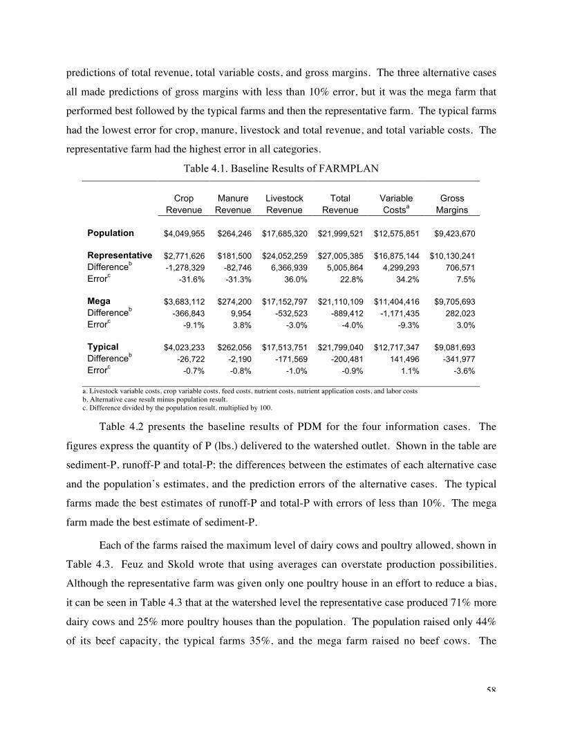
58
predictions of total revenue, total variable costs, and gross margins. The three alternative cases
all made predictions of gross margins with less than 10% error, but it was the mega farm thatperformed best followed by the typical farms and then the representative farm. The typical farms
had the lowest error for crop, manure, livestock and total revenue, and total variable costs. Therepresentative farm had the highest error in all categories.
Table 4.1. Baseline Results of FARMPLAN
Crop Manure Livestock Total Variable Gross
Revenue Revenue Revenue Revenue Costsa Margins
Population $4,049,955 $264,246 $17,685,320 $21,999,521 $12,575,851 $9,423,670
Representative $2,771,626 $181,500 $24,052,259 $27,005,385 $16,875,144 $10,130,241Differenceb
-1,278,329 -82,746 6,366,939 5,005,864 4,299,293 706,571Errorc
-31.6% -31.3% 36.0% 22.8% 34.2% 7.5%
Mega $3,683,112 $274,200 $17,152,797 $21,110,109 $11,404,416 $9,705,693Differenceb
-366,843 9,954 -532,523 -889,412 -1,171,435 282,023Errorc
-9.1% 3.8% -3.0% -4.0% -9.3% 3.0%
Typical $4,023,233 $262,056 $17,513,751 $21,799,040 $12,717,347 $9,081,693Differenceb
-26,722 -2,190 -171,569 -200,481 141,496 -341,977Errorc
-0.7% -0.8% -1.0% -0.9% 1.1% -3.6%
a. Livestock variable costs, crop variable costs, feed costs, nutrient costs, nutrient application costs, and labor costs b. Alternative case result minus population result. c. Difference divided by the population result, multiplied by 100.
Table 4.2 presents the baseline results of PDM for the four information cases. The
figures express the quantity of P (lbs.) delivered to the watershed outlet. Shown in the table aresediment-P, runoff-P and total-P; the differences between the estimates of each alternative case
and the population’s estimates, and the prediction errors of the alternative cases. The typicalfarms made the best estimates of runoff-P and total-P with errors of less than 10%. The mega
farm made the best estimate of sediment-P.
Each of the farms raised the maximum level of dairy cows and poultry allowed, shown inTable 4.3. Feuz and Skold wrote that using averages can overstate production possibilities.Although the representative farm was given only one poultry house in an effort to reduce a bias,
it can be seen in Table 4.3 that at the watershed level the representative case produced 71% more
dairy cows and 25% more poultry houses than the population. The population raised only 44%of its beef capacity, the typical farms 35%, and the mega farm raised no beef cows. The

59
representative farm had no beef capacity. The low level of beef production was a result of the
relatively low profitability of the activity.
Table 4.2. Baseline Phosphorous Deliveriesa for the Four Information Cases
Sediment
P [lbs]RunoffP [lbs]
TotalP [lbs]
Population 10,829 21,035 31,865
Representative 16,502 19,741 36,243
Differenceb5,672 -1,294 4,378
Errorc52.4% -6.2% 13.7%
Mega 14,071 11,628 25,698Differenceb
3,241 -9,408 -6,167Errorc
29.9% -44.7% -19.4%
Typical 14,216 20,313 34,530Differenceb
3,387 -722 2,665Errorc
31.3% -3.4% 8.4%
a. P delivered to the watershed outlet annually b. Alternative case result minus population result c. Difference divided by population result, multiplied by 100
Table 4.4 presents feed and livestock costs for each scenario. Livestock variable costs(which exclude feed and labor expenses) made up an average of 41% of total variable costs for
each of the cases followed by feed expenditures which accounted for 33% of total variable costs.
The ability to implicitly transfer resources—across farm boundaries—enabled the mega farm torealize an average of 19% lower feed costs than the population. Farm-raised feed was not
counted in feed expenditures. The mega farm was able to meet more total livestock requirementsfrom home-raised feed. The representative farm’s relatively high livestock costs are a direct
result of its higher levels of output.

60
Table 4.3. Livestock Capacities and Baseline Levels
DairyLevela
DairyCapacitya
BeefLevela
BeefCapacitya
PoultryLevelb
PoultryCapacityb
Population 4,240 4,240 1,210 2,750 97 97
Representative 7,260 7,260 0 0 121 121
Mega 4,240 4,240 0 2,750 97 97
Typical 4,240 4,240 952 2,750 95 95
a. One unit equals one cow. b. One unit equals one house.
Table 4.4. Feed Expenditures and Livestock Variable Costs
Livestock Total
Feed Variable LivestockExpenditures Costs Costsa
BaselinePopulation $4,284,189 $5,005,442 $9,289,631Representative $6,008,948 $7,021,122 $13,030,070Mega $3,427,454 $4,907,015 $8,334,469
Typical $4,264,900 $4,968,353 $9,233,253
Nutrient ManagementPopulation $3,986,327 $5,016,089 $9,002,415Representative $5,949,434 $7,021,122 $12,970,556Mega $3,429,388 $4,907,015 $8,336,404Typical $3,978,981 $4,977,272 $8,336,404
BufferPopulation $4,432,765 $5,024,056 $9,456,821Representative $6,002,718 $7,021,122 $13,023,840Mega $3,477,854 $4,907,015 $8,384,869Typical $4,415,605 $4,990,103 $9,405,708
a. Excluding labor costs.
The levels of crop rotations for each case-scenario are shown in Table 4.5. In thebaseline, the population, representative and mega farm cases put 85% of crop land in the corn
silage and alfalfa rotation because alfalfa was profitable as a cash crop in addition to being a feed
source for dairy cows. The typical farms put 95% of their crop land in the corn silage and alfalfarotation.
Table 4.6 presents nutrient expenditures and crop variable costs. Crop variable costs(which exclude nutrient, application and labor expenses) accounted for an average of 21% of

61
total variable costs while nutrient expenditures varied from 0 to 1% of total variable costs. Only
the population and typical farms purchased turkey litter and commercial N and potash in thebaseline, and none of the farms purchased commercial phosphate. Table 4.7 shows the levels of
P applied and removed by each information case under each of the three policy scenarios. Therepresentative and mega farms were able to meet all crop nutrient requirements through
applications of manure and litter produced on the farm. In the cases of the population and typical
farms beef and dairy farms purchased fertilizers, turkey litter and commercial N and potash. Thebeef farms (beef only, not with poultry) produced no recoverable manure and therefore had to
purchase crop nutrients. The beef farms applied turkey litter to corn silage to meet crop K and Prequirements, and applied commercial fertilizer to meet N requirements. The beef farms applied
turkey litter to alfalfa and pasture to meet crop P and N requirements, and applied commercial
potash to meet crop K requirements. The dairy farms were able to meet crop P needs withmanure applications, but the applications failed to satisfy all N and K requirements. The dairy
farms applied dairy manure to meet all nutrient requirements, and purchased turkey litter,
commercial N and potash to make up shortfalls on a crop and field basis.
Table 4.5. Crop Rotation Levels [acres] for Each Case-Scenario
Baseline CTCSa CTCSRYEb CTCSALFc PERMPASTd BUFFNARe Total
Population 408.5 235.4 9,559.6 1,008.2 0.0 11,211.7
Representative 0.0 1,464.1 9,752.6 0.0 0.0 11,216.7f
Mega 536.0 140.6 9,565.2 969.9 0.0 11,211.7
Typical 315.6 15.9 10,727.3 170.4 0.0 11,229.2f
NMPPopulation 737.4 2,464.5 7,063.2 516.8 0.0 10,781.9
Representative 0.0 4,888.4 6,328.3 0.0 0.0 11,216.7f
Mega 621.5 61.3 9,565.2 963.7 0.0 11,211.7
Typical 885.3 3,235.7 7,108.2 0.0 0.0 11,229.2f
BufferPopulation 375.0 188.1 8,750.5 710.4 1,187.7 11,211.7
Representative 0.0 1,839.2 8,107.0 0.0 1,270.5f 11,216.7f
Mega 460.8 265.0 8,756.0 542.2 1,187.7 11,211.7
Typical 313.2 9.0 9,581.2 111.6 1,214.2f 11,229.2f
a. Conventional-till Corn Silage b. Conventional-till Corn Silage and Rye Silage c. Conventional-till Corn Silage and Alfalfa d. Permanent Pasture e. Buffer f. Differences from population were caused by rounding errors when averaging resources and aggregating to watershed levels.

62
Table 4.6. Nutrient Expenditures and Crop Variable Costs
Crop Total
Nutrient Non-Nutrient CropExpenditures Costsa Costsb
BaselinePopulation $123,977 $3,067,423 $3,191,400Representative $0 $3,685,239 $3,685,239Mega $0 $3,022,958 $3,022,958Typical $117,882 $3,271,718 $3,389,600
Nutrient ManagementPopulation $221,043 $3,135,293 $3,356,336Representative $137,940 $3,923,806 $4,061,746Mega $6,933 $3,016,364 $3,023,297Typical $246,972 $3,484,657 $3,731,629
BufferPopulation $120,806 $2,879,216 $3,000,022
Representative $0 $3,426,670 $3,426,670Mega $0 $2,877,368 $2,877,368Typical $112,743 $3,015,240 $3,127,983
a. Crop variable costs plus nutrient application costs. b. Excluding labor costs.
Table 4.7. Phosphorous Applications and Removal
Phosphorous [lbs]
Applied Removed Excessa
BaselinePopulation 514,690 362,555 152,135Rep 489,324 387,959 101,365Mega 285,777 363,931 -78,154Typical 504,508 352,690 151,819
NMPPopulation 410,385 430,516 -20,131Rep 489,324 489,324 0Mega 285,777 363,151 -77,373Typical 442,738 459,675 -16,936
BufferPopulation 505,612 328,925 176,687
Rep 489,324 359,088 130,236Mega 285,777 336,982 -51,204Typical 492,592 315,632 176,960
a. P applied minus P removed

63
4.3 Nutrient Management Results
The nutrient management policy requires that field P applications not exceed P removed
by crops. Although allowable P applications could increase by selecting crops with higher Premoval rates, it was expected that reductions in P applications would be the method by which
the standard was mostly met. Therefore, it was expected that the nutrient management policy
would have the most significant effect on runoff-P.Table 4.8 presents the results of FARMPLAN for each of the information cases under the
nutrient management scenario. Nutrient management plan writing costs are shown in the table
and are subtracted from total revenue along with variable costs to derive gross margins. Thetypical farms made the best estimate of gross margins followed by the mega farm and then the
representative farm. All three cases grossly overestimated manure revenue with errors in excessof 1,000%. Because dairy manure is sold at a negative price, manure exported by farms in the
population to meet the nutrient management requirement was the cause of the decrease in
manure revenue by the farms. The representative and mega farms overestimated manure revenuebecause they did not have to export dairy manure to satisfy the nutrient management constraint.
Although the typical farms also exported dairy manure, they did so at a much lower level, only23% of the quantity exported by the population. The mega and typical farms had errors of less
than 10% for total revenue and variable costs. The three alternative cases made almost identical
estimates of nutrient management plan writing costs.

64
Table 4.8. Nutrient Management Scenario Results of FARMPLAN
NMP
Crop Manure Livestock Total Variable Writing GrossRevenue Revenue Revenue Revenue Costsa Costs Margins
Population $3,661,749 -$1,523 $17,742,921 $21,403,147 $12,435,936 $60,163 $8,907,048
Representative $2,779,007 $181,500 $24,052,259 $27,012,766 $17,167,359 $62,557 $9,782,850Differenceb
-882,742 183,023 6,309,338 5,609,619 4,731,423 2,394 875,802Errorc
-24.1% 12,017% 35.6% 26.2% 38.0% 4.0% 9.8%
Mega $3,675,146 $274,200 $17,152,797 $21,102,143 $11,406,665 $62,561 $9,632,917Differenceb
13,397 275,723 -590,124 -301,004 -1,029,271 2,398 725,869Errorc
0.4% 18,104% -3.3% -1.4% -8.3% 4.0% 8.1%
Typical $3,752,802 $191,742 $17,562,004 $21,506,548 $12,757,309 $62,630 $8,686,609Differenceb
91,053 193,265 -180,917 103,401 321,373 2,467 -220,439Errorc
2.5% 12,690% -1.0% 0.5% 2.6% 4.1% -2.5%
a. Livestock variable costs, crop variable costs, feed costs, nutrient costs, nutrient application costs, and labor costsb. Alternative case result minus the population resultc. Difference divided by population result, multiplied by 100
Table 4.9 presents the results of PDM for the nutrient management scenario. The mega
farm made the best prediction of sediment-P while the typical farms made the best predictions ofrunoff-P. The representative and typical farms overestimated sediment-P because they put more
acres in the corn and corn and rye rotations, which have high C factors, than the population andthey overestimated runoff-P because they applied more P than the population. The mega farm
underestimated sediment-P because it put more acres in the corn and alfalfa and pasture
rotations, which have low C factors, than the population, and underestimated runoff-P because itapplied less P than the population.

65
Table 4.9. Phosphorous Deliveriesa Under the Nutrient Management Scenario
SedimentP [lbs]
RunoffP [lbs]
TotalP [lbs]
Population 14,343 17,111 31,454
Representative 19,398 19,793 39,191Differenceb
5,055 2,682 7,737Errorc
35.2% 15.7% 24.6%
Mega 14,061 11,629 25,690Differenceb
-282 -5,482 -5,764Errorc
-2.0% -32.0% -18.3%
Typical 19,363 17,936 37,298Differenceb
5,020 825 5,845Errorc
35.0% 4.8% 18.6%
a. P delivered to the watershed outlet b. Alternative case result minus the population result c. Difference divided by the population result, multiplied by 100
Table 4.10 shows the compliance costs and changes in total-P of each information case
for the nutrient management scenario. The population predicted that implementing the nutrientmanagement policy throughout the watershed would cost farmers an aggregate of $516,622 and
would cause a decrease in P deliveries to the watershed outlet of 411 lbs; which equates to a
5.5% decrease in gross margins and a 1.3% decrease in total-P, or $1,257 per lb. Each of thealternative cases underestimated compliance costs, mostly by not predicting the decreases in crop
and manure revenue realized by the population. The representative and typical farms alsopredicted increases in total-P, while the mega farm estimated a decrease of only 0.03%, which
with a cost of $72,776 equates to $8,612 per lb. The representative farm experienced increases
in both sediment-P and runoff-P due to changes in crop rotations. The typical farms similarlyexperienced increases in sediment-P because of changes in crop rotations, but were able to
partially offset them with decreases in runoff-P caused by reductions in manure applications.The mega farm made few changes to crop rotations and no changes to manure applications. The
typical farms made the best estimate of compliance costs and the mega farm made the best
estimate of the change in total-P. A breakdown of the nutrient management compliance costs isshown in Table 4.11 as the changes in crop, manure and livestock revenue; the change in
variable costs; and the nutrient management plan writing costs. The changes and plan writing
costs can be summed to derive compliance costs. A breakdown of the changes in P deliveries is

66
shown in Table 4.12. For example, in the population case, sediment-P increased 3,513 lbs. while
runoff-P declined 3,924 lbs., for a net reduction of 411 lbs.The following sections provide a more detailed breakdown of the changes experienced by
each information case resulting from nutrient management.
Table 4.10. Compliance Costs and P Delivery Effects of the Nutrient Management Policy
Compliance Change in P
Costs Delivery [lbs]
Population $516,622 -411
Representative $347,391 2,948Differencea
-169,231 3,359Errorb
-32.8% 817.2%
Mega $72,776 -8Differencea
-443,846 403Errorb
-85.9% 97.9%
Typical $395,084 2,769Differencea
-121,538 3,180Errorb
-23.5% 773.6%
a. Alternative case result minus the population result b. Difference divided by the population result, multiplied by 100
Table 4.11. Breakdown of the Nutrient Management Compliance Costs
Changea Changea Changea Changea NMPin Crop in Manure in Livestock in Variable Writing Compliance
Revenue Revenue Revenue Costs Costs Costsb
Population -$388,206 -$265,769 $57,601 -$139,915 $60,163 $516,622Representative $7,381 $0 $0 $292,215 $62,557 $347,391Mega -$7,966 $0 $0 $2,249 $62,561 $72,776
Typical -$270,431 -$70,314 $48,253 $39,962 $62,630 $395,084
a. Nutrient management results minus baseline results b. Compliance costs equal gross margins from the baseline scenario minus gross margins under the nutrient management policy. Equivalently, compliance costs = NMP writing costs + change in variable costs – change in crop revenue – change in manure revenue – change in livestock revenue.

67
Table 4.12. Changes in P Deliveries [lbs] Under the Nutrient Management Policy
Sediment-P Runoff-P Total-P
Population 3,513 -3,924 -411Representative 2,896 52 2,948Mega -10 1 -8Typical 5,146 -2,378 2,769
4.3.1 Population
In the baseline, the population applied 152,135 lbs. of excess P (P applied to fields minus
P removed by crops). In the nutrient management scenario the population reduced the number ofacres of pasture and the conventional-till corn silage and alfalfa rotation, and increased the
number of acres in the conventional-till corn silage and rye silage rotation and the conventional-till corn silage rotation. The change in crop mix resulted in an increase of 67,961 lbs. of P
removed by crops. For example, field 9, which belongs to a small dairy-with-poultry, shifted all
of its 36.9 acres from the corn and alfalfa rotation to the corn and rye rotation, resulting in anincrease in P removed of 935 lbs., or 77%. The change in rotations also caused the loss of crop
revenue because sales of the higher priced alfalfa were replaced by corn silage, but also led to anet decrease in feed expenditures—savings were made through reductions in the purchase of
corn silage. Other economic effects of the crop changes were higher crop variable costs and
lower labor costs. Farms removed 431.8 acres of low yielding crop land from production, whichwere assigned to PDM as farmstead and given the appropriate factors. The changes to crop
rotations (shifts away from alfalfa and pasture toward more corn silage and rye silage) were thecause of the increase in sediment-P. The average (weighted by acres) C factor and alpha
increased 36.6% and 10.5%, respectively, causing increases in gross erosion and sediment
delivery. They also caused runoff/acre and beta to increase 23.6% and 55.1%, respectively,leading to 248 lbs. of additional runoff-P. For example, field 942 saw the following changes: 1)
the C factor increased from 0.094 to 0.214; 2) alpha increased from 5.1 to 6.2; 3) runoffincreased from 2.17 to 7.68 inches/acre; and 4) beta increased from 5.3 to 12.4. Consequently,
field 942 realized the following sediment and runoff changes: 1) gross erosion increased 30,526
lbs./acre; 2) sediment delivered increased 6,014 lbs./acre; 3) runoff increased 1.25 millionlbs./acre; and 4) runoff delivered increased 616,099 lbs./acre.

68
The population reduced P applications by 104,305 lbs. by decreasing the quantity of dairy
manure and turkey litter spread. The farms were forced to sell a total of 10,103,300 gallons ofdairy manure (44,770 lbs. of P) at a cost of $266,728 to meet the nutrient management
requirement. It was assumed that a market exists within 60 miles to purchase dairy manure. Thereductions accounted for 94% of the change in runoff-P, or 4,172 lbs. Manure was spread in the
baseline mostly to meet crop N and K requirements, which often resulted in over applications of
P; however, there were some occasions where some manure was spread for disposal purposes,meaning all nutrients were over applied. In the nutrient management scenario the farms were
forced to purchase additional commercial fertilizers at a cost of $97,066. Commercial fertilizerscost less to apply than manure and litter, therefore the change in nutrient sources allowed the
farms to realize a decrease in application costs.
In the nutrient management scenario the population realized a deficit of 20,131 lbs. of P.Deficits can occur when the level of P removed by crops is greater than recommended crop P
applications, allowing the farm to apply less P than is removed because nutrient constraints
require farms to apply levels to meet crop requirements not removal. In the baseline, some farmsrealized a deficit, which were offset by surpluses on other farms. In the nutrient management
scenario the overall deficit occurred because farms could no longer have surpluses. Individualfarms that realized a deficit did not sell any dairy manure. In the nutrient management scenario,
the farms also increased the level of beef cows by 131, raising both livestock variable costs and
revenue. The increase in beef levels was a result of the change in crop selection. Corn and ryeboth require fewer hours of labor than alfalfa. When the farms switched from alfalfa to corn and
rye to increase crop P removed, labor resources became available and allowed the increase inbeef levels.
4.3.2 Representative Farm
In the baseline, the representative farm, at the watershed level, applied 101,365 lbs. of
excess P. In the nutrient management scenario the farm decreased the number of acres of theconventional-till corn silage and alfalfa rotation and replaced them with the conventional-till
corn silage and rye silage rotation (see Table 4.5), increasing crop P removed by 101,365 lbs.Crop revenue and variable costs increased, and feed expenditures and labor costs decreased. The
effects on sediment were the same as in the population case, the C factor average increased
33.5% and the alpha average increased 6.4%, causing increased gross erosion and sediment

69
delivery. Average runoff/acre increased 23.4% while the average value of beta increased 60.5%.
The total effect, as can be seen in Table 4.12, was an increase in runoff-P of 52 lbs.The representative farm also redistributed manure applications among the fields because
in the baseline some fields had a deficit of P. However, the farm was not forced to reduce theaggregate quantity of applied P, so runoff-P was mostly unchanged from the baseline. The
adjustments to crop rotations and manure applications resulted in a need for commercial N that
cost the farm $137,940. In the nutrient management scenario, the representative farm balanced Papplications with crop P removal, and made no changes to livestock activities.
4.3.3 Mega Farm
The mega farm experienced a P deficit of 78,154 lbs. in the baseline, but had some fieldsthat had excess P because dairy manure was spread to meet crop N requirements. In the nutrient
management scenario the mega farm made insignificant changes to crop rotations (see Table
4.5), its decrease in crop revenue (see Table 4.11) was a result of an increase in corn silage usedfor feed which reduced the quantity available for sale. The nutrient management requirement
was met by transferring the excess P to the fields with deficits. The mega farm was also requiredto purchase commercial N at a cost of $6,933. The farm made no changes to its livestock
activities.
4.3.4 Typical Farms
In the baseline, the typical farms applied 151,819 lbs. of excess P. By moving someacres from permanent pasture and conventional-till corn silage and alfalfa rotation to the
conventional-till corn silage and rye silage rotation (see Table 4.5), the farms were able toincrease P removed by crops by 106,985 lbs. Those changes resulted in higher levels of corn and
rye silage, and lower levels of alfalfa and grass. Although the farms increased purchases of corn
grain and alfalfa, they were able to lower feed expenditures by decreasing the level of corn silagepurchased, a result of the increase in corn silage grown. Decreased alfalfa sales more than offset
increased corn silage sales and the farms realized lower crop revenue. In addition, crop variablecosts increased and labor costs decreased. The effects of the crop changes on sediment-P were
even more pronounced than those of the population. The average values of the C factor and
alpha increased 47.4% and 11.6%, respectively, driving up gross erosion, sediment delivered,

70
and therefore sediment-P. Average runoff/acre and beta increased 30.7% and 75.3%,
respectively, leading to an increase in runoff-P of 93 lbs.The farms decreased P applications by 61,770 lbs. by reducing the levels of dairy manure
and turkey litter spread on the fields. The farms were forced to sell 2,666,000 gallons of dairymanure (11,814 lbs of P) at a cost of $70,390. The decrease in applications resulted in a
decrease in runoff-P of 2,471 lbs (Table 4.12). The farms were also forced to purchase
additional N and potash at a cost of $129,090, although application costs fell by $13,884. Thetypical farms increased beef levels by 87 units, leading to increases in livestock revenue and
variable costs. As in the population case, the increase in beef production was a result of thechange in crop selection from alfalfa to corn and rye, which freed some labor for beef activities.
4.4 Buffer Scenario Results
Because buffer strips are a land use practice, all the land use coefficients are affected.From Table 3.13 it can be seen that buffers have the lowest C factor, alpha and runoff
coefficient; and the second lowest beta value of all the rotations. Land that is converted fromone of the rotations other than pasture, which has the same coefficients as buffers, would realize
reductions in delivered sediment and runoff. More significant is the trapping effect the buffers
have on sediment and runoff. Since sediment and runoff from all the fields must pass through abuffer, the average delivery ratios of the non-buffer fields for sediment and runoff would
decrease. Table 3.19 shows that the average sediment and runoff delivery factors of the non-buffer fields for the population decreased by 39.4% and 35%, respectively. The majority of
runoff-P is comprised of applied-P, and the losses of applied-P are unaffected by land use;
therefore it was expected that the buffers would have the greatest effect on sediment-P.Table 4.13 presents the results of FARMPLAN for each of the information cases under
the buffer policy scenario. The mega farm made the best estimate of gross margins followed bythe typical farms and the representative farm. The typical farms underestimated all revenues
while the mega farm underestimated everything but manure revenue and gross margins. The
representative farm overestimated livestock and total revenue, variable costs, and gross margins.As in the baseline scenario, the typical farm made the best estimates of variable costs and total
revenue.

71
Table 4.13. Buffer Scenario Results of FARMPLAN
Crop Manure Livestock Total Variable Gross
Revenue Revenue Revenue Revenue Costsa Margins
Population $3,659,939 $265,134 $17,786,029 $21,711,102 $12,548,082 $9,163,020
Representative $2,210,428 $181,500 $24,052,259 $26,444,187 $16,598,538 $9,845,649Differenceb
-1,449,511 -83,634 6,266,230 4,733,085 4,050,456 682,629Errorc
-39.6% -31.5% 35.2% 21.8% 32.3% 7.4%
Mega $3,323,957 $274,200 $17,152,797 $20,750,954 $11,301,710 $9,449,244Differenceb
-335,982 9,066 -633,232 -960,148 -1,246,372 286,224Errorc
-9.2% 3.4% -3.6% -4.4% -9.9% 3.1%
Typical $3,549,272 $262,960 $17,631,447 $21,443,679 $12,623,712 $8,819,967Differenceb
-110,667 -2,174 -154,582 -267,423 75,630 -343,053Errorc
-3.0% -0.8% -0.9% -1.2% 0.6% -3.7%
a. Livestock variable costs, crop variable costs, feed costs, nutrient costs, nutrient application costs, and labor costs b. Alternative case result minus the population result c. Difference divided by population result, multiplied by 100
Table 4.14 presents the results of PDM for the four information cases under the bufferscenario. The typical farms made the best estimate of runoff-P and total-P, and the second best
estimate of sediment-P. The representative farm had the best estimate for sediment-P. The
representative and mega farms underestimated sediment-P and runoff-P, and hence total-P, whilethe typical overestimated sediment-P and total-P, and underestimated runoff-P.
Table 4.15 shows the compliance costs and changes in total-P of each information casefor the buffer scenario. The population case predicted that implementing the buffer policy would
cost the farms an aggregate of $260,650 and would decrease P deliveries by 1,499 lbs; whichequates to a 2.8% decrease in gross margins and a 4.7% decrease in total-P, and a cost of
$173.87 per lb. The typical farms made the best estimate of compliance costs and the change in
total-P. All three cases grossly overestimated the reduction in total-P with errors in excess of100%, and the cost effectiveness of the buffer policy. The representative farm predicted a cost of
$39.97 per lb., the mega farm predicted $45.13 per lb. and the typical farms predicted $66.49 perlb. The overestimate in cost effectiveness was a result of the overestimate in the reduction of
total-P which was driven by overestimates of the reduction in sediment-P. The overestimates in
the reduction of sediment-P were caused by overestimates in sediment delivery and were a result

72
of using a simplified version of PDM for the alternative cases, and the method by which the
delivery factors (D and B) were estimated and assigned.
Table 4.14. Phosphorous Deliveriesa for the Buffer Scenario
SedimentP [lbs]
RunoffP [lbs]
TotalP [lbs]
Population 9,701 20,665 30,366
Representative 9,428 19,695 29,123Differenceb
-273 -969 -1,242Errorc
-2.8% -4.7% -4.1%
Mega 8,434 11,581 20,015Differenceb
-1,267 -9,084 -10,350Errorc
-13.1% -44.0% -34.1%
Typical 10,754 19,840 30,593Differenceb
1,053 -825 228
Errorc10.9% -4.0% 0.8%
a. P delivered to the watershed outlet b. Alternative case results minus the population results c. Difference divided by the population result, multiplied by 100
The breakdown of the buffer compliance costs and P deliveries are shown in tables 4.16
and 4.17, respectively. Compliance costs were driven by the loss of crop revenue due to the lossof crop land to the buffers. The buffers had lower variable costs than the crops which helped to
partially offset the loss in revenue. The population and typical farms were also able to allocate
labor that was freed up by the mandatory buffers to beef activities which also helped to reducethe compliance costs.
A detailed breakdown of the results for each information case is provided in thefollowing sections.

73
Table 4.15. Compliance Costs and P Delivery Effects of the Buffer Policy
Compliance Change in P
Costs Delivery [lbs]
Population $260,650 -1,499
Representative $284,592 -7,120Differencea
23,942 -5,620Errorb
9.2% -374.9%
Mega $256,449 -5,683Differencea
-4,201 -4,184Errorb
-1.6% -279.1%
Typical $261,726 -3,936Differencea
1,076 -2,437Errorb
0.4% -162.6%
a. Alternative case result minus the population result b. Difference divided by the population result, multiplied by 100
Table 4.16. Breakdown of the Buffer Policy Compliance Costs
Changea Changea Changea Changea
in Crop in Manure in Livestock in Variable Complianceb
Revenue Revenue Revenue Costs Costs
Population -$390,016 $888 $100,709 -$27,769 $260,650Representative -$561,198 $0 $0 -$276,606 $284,592Mega -$359,155 $0 $0 -$102,706 $256,449
Typical -$473,961 $904 $117,696 -$93,635 $261,726
a. Buffer scenario results minus the baseline results b. Compliance costs equal gross margins from the baseline scenario minus gross margins under the nutrient management policy.
Equivalently, compliance costs = change in variable costs – change in crop revenue – change in manure revenue – change in livestock revenue.
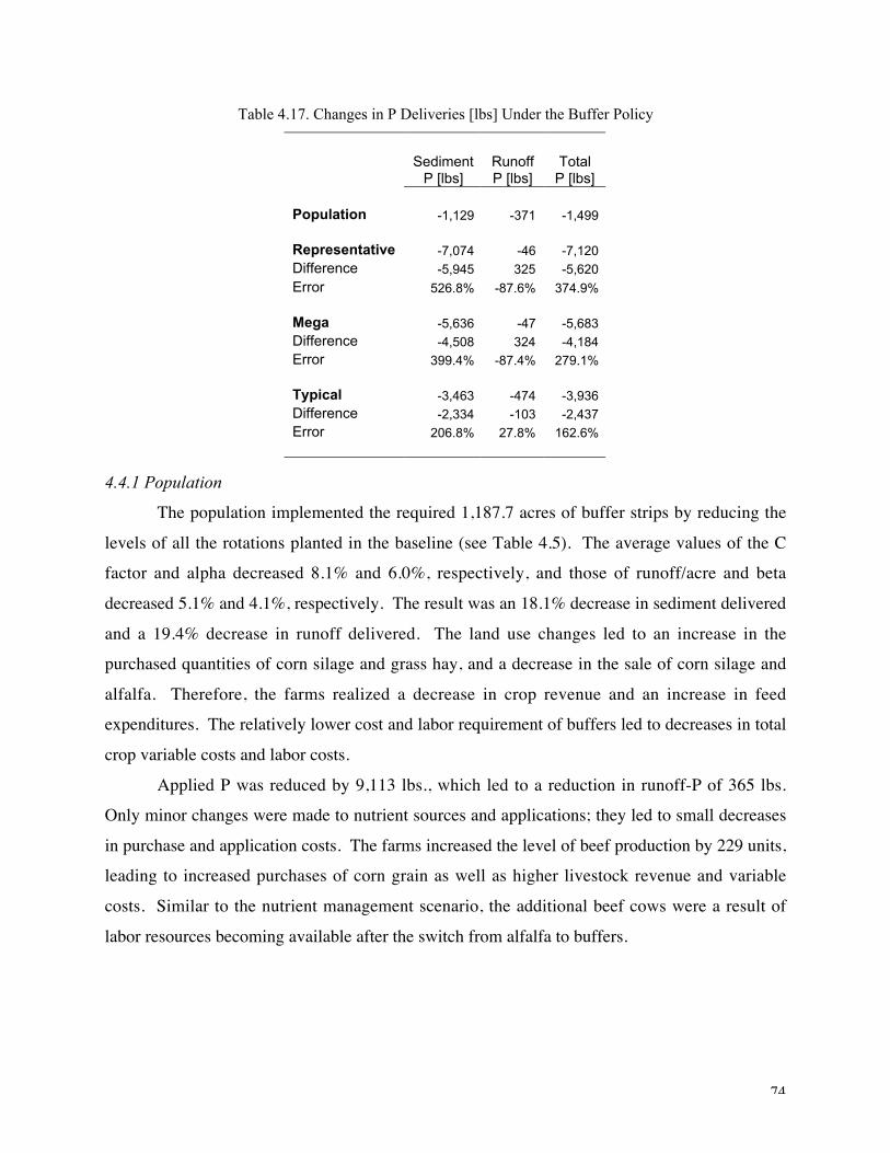
74
Table 4.17. Changes in P Deliveries [lbs] Under the Buffer Policy
SedimentP [lbs]
RunoffP [lbs]
TotalP [lbs]
Population -1,129 -371 -1,499
Representative -7,074 -46 -7,120Difference -5,945 325 -5,620
Error 526.8% -87.6% 374.9%
Mega -5,636 -47 -5,683Difference -4,508 324 -4,184Error 399.4% -87.4% 279.1%
Typical -3,463 -474 -3,936Difference -2,334 -103 -2,437Error 206.8% 27.8% 162.6%
4.4.1 Population
The population implemented the required 1,187.7 acres of buffer strips by reducing the
levels of all the rotations planted in the baseline (see Table 4.5). The average values of the Cfactor and alpha decreased 8.1% and 6.0%, respectively, and those of runoff/acre and beta
decreased 5.1% and 4.1%, respectively. The result was an 18.1% decrease in sediment delivered
and a 19.4% decrease in runoff delivered. The land use changes led to an increase in thepurchased quantities of corn silage and grass hay, and a decrease in the sale of corn silage and
alfalfa. Therefore, the farms realized a decrease in crop revenue and an increase in feedexpenditures. The relatively lower cost and labor requirement of buffers led to decreases in total
crop variable costs and labor costs.
Applied P was reduced by 9,113 lbs., which led to a reduction in runoff-P of 365 lbs.Only minor changes were made to nutrient sources and applications; they led to small decreases
in purchase and application costs. The farms increased the level of beef production by 229 units,leading to increased purchases of corn grain as well as higher livestock revenue and variable
costs. Similar to the nutrient management scenario, the additional beef cows were a result of
labor resources becoming available after the switch from alfalfa to buffers.

75
4.4.2 Representative Farm
Errors resulted from averaging population resources and aggregating farm results and led
to the representative farm reporting 1,270.5 acres of buffer compared to 1,187.7 acres for thepopulation. Those acres, plus 375 additional acres of conventional-till corn silage and rye silage,
were grown in place of conventional-till corn silage and alfalfa. Changes in land use led to a
61.9% decrease in sediment delivered and a 29.3% decrease in runoff delivered. Losses inalfalfa revenue were partially offset by gains in corn silage revenue for a net decrease in crop
revenue. In addition, an increase in the purchase of corn grain led to higher feed expenditures;
and crop variable costs decreased. Total P applications remained unchanged, isolating theeffects, if small, of the buffers on runoff-P. No changes were made to livestock or other nutrient
activities.
4.4.3 Mega Farm
In addition to the 1,187.7 acres of buffer, the mega farm changed crop rotations by
increasing the acreage under the conventional-till corn silage and rye silage rotation. The resultswere decreases in sediment and runoff delivered of 40.2% and 23.8%, respectively. The farm
made small increases in the purchased levels of corn grain and grass hay, increasing feed
expenditures, and decreases in the levels of corn silage and alfalfa sold, decreasing crop revenue.Crop variable costs and labor expenses decreased as a result of the land use changes. Like the
representative farm, the mega farm made no changes to the level of applied P, and therefore the
relatively small decrease in runoff-P was a result of the buffers. The farm made no changes to itslivestock or other nutrient application activities.
4.4.4 Typical Farms
As in the representative farm case, averaging and aggregation errors resulted in thetypical farms reporting 1,214.2 acres of buffer. The buffers came mostly at the expense of the
conventional-till corn silage and alfalfa rotation (see Table 4.5). The land use change led to adecrease in the delivery of sediment of 27.1% and a decrease of runoff delivered of 2.2%. The
loss of feed crops resulted in additional purchases, and lower sales, of corn silage and grass hay,
resulting in higher feed costs and lower crop revenue along with lower crop variable costs andlabor expenses.

76
The farms reduced the levels of commercial N and potash purchased, which resulted in
lower nutrient and application costs. The farms also reduced P applications by 11,917 lbs.,which led to a decrease in runoff-P of 474 lbs. Like the population, the typical farms increased
the level of beef cows, by 245 units. Again, the additional beef cows were a result of freed laborresources after the switch from alfalfa to buffers. That change led to increased quantities of
purchased corn grain, and higher livestock revenue and variable costs.
4.5 Summary
All the information cases raised the maximum level of dairy cows and poultry in all the
scenarios. Beef operations were limited by low profitability. Only a small number of acres wereleft out of production, occurring only for the population in the nutrient management scenario.
Farms in all information cases were able to use most dairy manure and poultry litter to meet crop
nutrient needs, although in doing so one or more nutrients were often exceeded; e.g. manure wasapplied to corn silage to meet crop N needs while P and K applications exceeded
recommendations. In addition, there were some cases of dairy-with-broilers where applicationsof all three nutrients exceeded recommendations. Table 4.18 shows the rankings of the errors of
the three alternative cases for the baseline predictions of total revenue, total variable costs, gross
margins, sediment-P, runoff-P and total-P. The typical farms ranked first four times, includingtotal-P, and did not rank third in any category. The mega farm clearly performed second to the
typical farm, but did have the top ranking for the estimates of gross margins and sediment-P.
Table 4.18. Ranking of Errors for Baseline Predictions
Total Total Gross
Revenue Variable Costs Margins Sediment-P Runoff-P Total-P
Representative 3rd 3rd 3rd 3rd 2nd 2nd
Mega 2nd 2nd 1st 1st 3rd 3rd
Typical 1st 1st 2nd 2nd 1st 1st
In the nutrient management scenario, the population, representative and typical farms
shifted production from highly profitable alfalfa to higher P-consuming corn and rye silage. The
change in crop levels led to increases in sediment-P, which limited the effectiveness of thepolicy. All the information cases were forced to purchase additional quantities of commercial N

77
and potash. The population and typical farms were forced to sell dairy manure at a loss in order
to reduce P applications. The shift in crop rotations and the exportation of dairy manureaccounted for most of the compliance costs. Decreases in manure, and therefore P, applications
by the population and typical farms accounted for the decreases in runoff-P.Table 4.19 shows the rankings of the predictions made in the nutrient management
scenario and Table 4.20 shows the rankings of the changes between the baseline and nutrient
management scenarios. The typical farms performed best, ranking first seven times and secondfive times; however, two of the second place rankings were for the predictions of total-P. These
rankings partially support the first proposition made in section 1.7, that the typical farms wouldyield the most accurate predictions of compliance costs and pollution reductions (total-P),
followed by the mega farm. The mega farm made the best prediction of total-P reductions, but
the typical farms made the best estimate of compliance costs, reflected in the rankings of thechange in gross margins shown in Table 4.20 (or see the results in Table 4.10). In addition, the
typical farms made changes that more closely resembled those of the population: changes in land
use, changes in nutrient applications and the sale of dairy manure, and changes to beef levels.
Table 4.19. Ranking of Errors for Nutrient Management Predictions
Total Total Gross
Revenue Variable Costs Margins Sediment-P Runoff-P Total-P
Representative 3rd 3rd 3rd 3rd 2nd 3rd
Mega 2nd 2nd 2nd 1st 3rd 1st
Typical 1st 1st 1st 2nd 1st 2nd
Table 4.20. Ranking of Errors for Changes Between the Baseline and Nutrient Management
Scenarios
Total Total Gross
Revenue Variable Costs Margins Sediment-P Runoff-P Total-P
Representative 3rd 3rd 3rd 1st 3rd 3rd
Mega 2nd 1st 2nd 3rd 2nd 1st
Typical 1st 2nd 1st 2nd 1st 2nd

78
In the buffer scenario, for all information cases, most of the buffer acres came at the
expense of the corn silage and alfalfa rotation. The buffers were successful in reducing thequantities of sediment and runoff delivered, as well as the associated P. The population and
typical farms also reduced P applications, which led to further decreases in runoff-P.Compliance costs were mostly comprised of losses in alfalfa sales, but partially offset by lower
variable costs.
Table 4.21 shows the rankings of the predictions made in the buffer scenario and Table4.22 shows the rankings of the changes between the baseline and buffer scenarios. The typical
farms again performed best with ten first place and two-second place rankings. In this scenario,the first proposition stated in section 1.7 regarding the rankings of information cases was
completely validated with the typical farm making the best estimate of the changes in all
categories, and the mega farm making the second best estimates. As in the nutrient managementscenario, the production changes made by the typical farms were more like those of the
population than were the changes made by the other two cases.
Table 4.21. Ranking of Errors for Buffer Predictions
Total Total Gross
Revenue Variable Costs Margins Sediment-P Runoff-P Total-P
Representative 3rd 3rd 3rd 1st 2nd 2nd
Mega 2nd 2nd 1st 3rd 3rd 3rd
Typical 1st 1st 2nd 2nd 1st 1st
Table 4.22. Ranking of Errors for Changes Between the Baseline and Buffer Scenarios
Total Total Gross
Revenue Variable Costs Margins Sediment-P Runoff-P Total-P
Representative 3rd 3rd 3rd 3rd 3rd 3rd
Mega 2nd 2nd 2nd 2nd 2nd 2nd
Typical 1st 1st 1st 1st 1st 1st
The second proposition made in section 1.7 was that the errors would be greater in thebuffer scenario than the nutrient management scenario (see Tables 4.10 and 4.15). This
proposition was validated in only one of the cases, the change in total-P errors for the mega farm.

79
In all the other cases, both for compliance costs and changes in total-P, errors were smaller in the
buffer scenario than the nutrient management scenario.Table 4.23 summarizes the errors of the predictions of compliance costs and change in
total-P for the three alternative cases for both the nutrient management and buffer scenarios.Each information case underestimated the compliance costs of the nutrient management policy
because they did not estimate the high level of dairy manure exported by the population. The
alternative cases overestimated the change in total-P; although the estimates were actuallyshortfalls in the prediction of the reduction of total-P, meaning that the alternative cases
predicted less of a reduction than the population (see Table 4.10). This was also in large part dueto the failure to estimate the dairy manure exports. Prediction errors for the compliance costs of
the buffer policy were much smaller than those of the nutrient management policy, while the
errors for the change in total-P were mixed in comparison to those of the nutrient managementscenario. The compliance costs were mostly a loss of crop revenue, a result of the loss of crop
land to buffers. Since the buffer acres were specified and not chosen by the model or
information cases, there were fewer policy responses for the alternative cases to predict relativeto the population than in the nutrient management scenario.
As discussed above, the proposition made in regards to the rankings of the informationcases was validated in ten of the twelve cases. The two exceptions being that 1) the
representative farm outperformed the mega farm in predicting the compliance costs of the
nutrient management policy, and 2) the mega farm outperformed the typical farm in predictingthe change in total-P caused by implementing the nutrient management policy.
Table 4.23. Prediction Errors For Each Alternative Case-Scenario
Nutrient Management Buffers
Compliance Change in Compliance Change inCosts Total-P Costs Total-P
Representative -32.8% 817.2% 9.2% -374.9%Mega -85.9% 97.9% -1.6% -279.1%Typical -23.5% 773.6% 0.4% -162.6%

80
Chapter 5 Summary and Conclusions
5.1 Introduction
In the state of Virginia, population growth and the associated increases in municipalwastewater, along with the threat of EPA regulations, will increase the need for reductions in P
loads in surface waters in order to meet and maintain water quality standards for the Chesapeake
Bay. Agriculture contributes 49% of P entering the Bay; therefore, it can be expected thatagriculture will be targeted as a source of P reductions. Livestock operations will be targeted in
particular because many of them are characterized as having excess nutrients generated on thefarm because they are unable to utilize on their crop land the amount of nutrients generated by
the livestock.
Spatially variable physical and socioeconomic characteristics of a watershed and itsoccupant farms affect both the decisions made by farmers and the transport of nutrients.
Historically, studies have used regional or national-scale representative farms to studyagricultural policies. Evidence (e.g. Feuz and Skold; Wu and Segerson; and Braden et al.)
suggests that spatially variable characteristics should be considered when designing policies to
control nonpoint sources of water pollution. However, spatial information can be expensive tocollect and the evidence is not conclusive as to what levels of information should be used for
analyzing specific pollution-control policies.The objective of this study was to estimate the accuracy of predicted compliance costs
and changes in P deliveries resulting from mandatory buffer installation and mandatory nutrient
management for three alternative cases using varying levels of information, relative to thepopulation of farms in a Virginia watershed. The first alternative case was a representative farm
described as a small dairy-with-poultry and given watershed averages of physical resources. Thesecond case was a mega farm that was given all the physical resources and livestock capacity of
the watershed. The third alternative case was a set of typical farms, one for each type of farm
(e.g. small dairy) in the watershed. Each typical farm was given the average resources of thegroup of farms of the corresponding type in the watershed.
For each information case, an economic model, FARMPLAN, was used to determine the
baseline profit maximizing levels of inputs, outputs and gross margins at the field (whereapplicable), farm and watershed levels. Selected crop rotations and P applications were used as

81
inputs to the physical model, PDM, which estimated the baseline levels of P delivered to the
watershed outlet (total-P). The process was repeated two times, once for each policyconstraint—nutrient management and buffers. The watershed levels of gross margins and total-P
(the sum of sediment-P and runoff-P) for the baseline were subtracted from those of the twopolicy scenarios to determine the compliance costs and effectiveness of the two policies. The
compliance cost and P reduction estimates made by the three alternative cases were compared to
those of the population, which was viewed as the case of “complete” information, to determinetheir accuracy. Prediction errors were calculated and compared to determine the accuracy of
each alternative case in making compliance cost and pollution estimates.
5.2 Results
5.2.1 Baseline
In the baseline, each of the information cases raised the production capacity level of dairy
cows and poultry. The representative farm, when aggregated to the watershed level, raised moredairy cows and poultry than the population. Beef production was limited due to the relatively
low profitability of the activity. The mega farm did not raise any beef, and was able to realize
lower feed expenditures than the population, and higher net crop revenue.Each of the cases put a large majority of crop land into a corn silage and alfalfa rotation,
selling much of the alfalfa for cash. None of the cases purchased commercial phosphate, andonly the population and typical farms purchased commercial N and potash. The population,
representative farm and typical farms each applied an excess quantity of P while the mega farm
applied a deficit.The typical farms made the best estimates of total revenue and total variable costs;
however, the mega farm made the best estimate of gross margins. The representative farmranked third in all three categories. The typical farms made the best estimates of runoff-P and
total-P, followed by the representative farm. The mega farm made the best estimate of sediment-
P followed by the typical farms.
5.2.2 Nutrient Management
The nutrient management policy required that field P applications not exceed P removed
by crops. The population, representative farm and typical farms each moved crop acres from

82
corn and alfalfa to corn and rye in order to increase the level of P removed by the crops. The
mega farm made minor changes because, although the farm as a whole realized a P deficit in thebaseline, some fields had surplus levels of P. Therefore, the mega farm had only to transfer P
applications in the form of manure from fields with a surplus to fields with a deficit. Thepopulation and typical farms made significant reductions to P applications, while the
representative and mega farms made no changes to the total quantity applied. All four
information cases were forced to purchase commercial N to meet crop needs. The populationand typical farms also had to purchase additional commercial potash, and pay to transport dairy
manure off some farms. Because they were able to apply all the dairy manure generated on thefarm, the representative and mega farms did not have to dispose of any manure off the farm. The
economic impact was mixed across information cases in terms of the changes in costs and
revenues. Compliance costs ranged from a low of $72,776 for the mega farm to a high of$519,622 for the population. The typical farms made the best prediction of compliance costs
followed by the representative farm and then the mega farm.
The population and typical farms experienced increases in sediment-P and decreases inrunoff-P. The population realized a net decrease in total-P while the typical farms realized a net
increase. The decreases in runoff-P were a result of the farms’ reduction in P applications, whichcontrolled 97% of runoff-P. The increases in sediment-P were a result of the changes in crop
rotations and their effects on gross erosion and sediment delivery. The representative farm
experienced increases in both sediment-P and runoff-P. The increase in runoff-P resultedbecause the changes in crop rotations led to increases in runoff and runoff delivered. If not for
the decreased P applications, the population and typical farms would have also experiencedincreases in runoff-P due to the effects of the change in crop rotations on average annual runoff
and runoff delivery. The mega farm realized minor changes to P deliveries; a decrease in
sediment-P, increase in runoff-P, and a net decrease in total-P.
5.2.3 Buffers
The buffers were implemented at the expense of the corn silage and alfalfa, permanent
pasture, and corn silage rotations. The population and typical farms also decreased acres of cornand rye silage while the representative and mega farms increased acres of that rotation. The
changes in rotations led to increased feed expenditures for all the information cases except the
representative farm, which realized a decrease. Because buffers have lower variable costs than

83
the other rotations, each of the information cases realized a decrease in crop variable costs. The
population and typical farms were also able to make minor reductions in the quantities ofcommercial N and potash purchased. Compliance costs ranged from $256,449 for the mega farm
to $284,592 for the representative farm. The typical farm made the best prediction followed bythe mega farm and then the representative farm.
The buffers led to reductions of both sediment-P and runoff-P for all four information
cases. Gross erosion and runoff were reduced on the fields where the buffers were implemented,but delivery reductions also resulted from the decrease in the average sediment delivery ratio and
the decrease in the average runoff delivery ratio experienced by the other fields, which drainedinto the buffers. The population and typical farms also realized decreases in runoff-P as a result
of lower P applications. Each of the alternative cases grossly overestimated the reduction in
total-P. The typical farm made the best prediction of the reduction followed by the mega farmand then representative farm.
5.2.4 Interpretation
The results support the proposition that the inclusion of greater levels of spatialinformation will lead to more accurate estimates of compliance costs and pollution reductions.
Not only did the set of typical farms make the best estimate of compliance costs for the nutrient
management policy, and compliance costs and P reductions for the buffer policy, but theirproduction decisions made in response to the policies tracked those of the population better than
the other two alternative information cases. The typical farms applied and removed quantities ofP similar to those of the population, and realized nearly the same quantity of excess P in the
baseline case. The typical farms were the only alternative case to purchase commercial N and
potash in the baseline, as did the population. The set of typical farms was the only alternativecase to sell dairy manure in response to the nutrient management policy, like the population. The
typical farms made the best estimate of compliance costs by making the closest approximations
to the changes in crop, livestock and manure revenue.The results from the representative farm demonstrate the potential weakness of
describing a region with one farm type. The major problem with the representative farm wasdeclaring that the average farm was a dairy-with-poultry, and then using its crop acreage to
assign livestock capacity. This caused the farm to greatly overstate dairy and poultry levels for
the watershed. Those overstatements led to poor estimates of crop and livestock revenue and

84
costs. Production possibilities can quickly become overstated. The bias in livestock levels was
somewhat reduced by giving the representative farm only one poultry house even though a smalldairy-with-poultry would normally have two houses. The representative farm still overstated
poultry production by 25%. In addition to over representing one activity, a representative farmcan under represent another. Sixty-two of the farms in the watershed have a combined capacity
for 2,750 beef cows; however, the representative farm, being a dairy-with-poultry, had no beef
cows. The conclusion is that using a single farm type to represent a watershed can save ininformation costs, but it will lead to inaccurate estimates of production levels, costs, revenues
and nutrient deliveries.It appears that the inclusion of farm boundaries is imperative to making quality estimates.
The mega farm included the full composition of physical resources and livestock capacity as the
population. But the lack of farm boundaries allowed the mega farm to assign the physicalresources to individual units of livestock in a manner that is not realistic, hence its predictions
were second to those of the typical farms more times than not. In no scenario did the mega farm
choose to raise beef cows even though the population and typical farms found reason to bring theactivity into production. The fact that the mega farm experienced a P deficit in the baseline is
another example of how a lack of farm boundaries allowed for unrealistic allocations ofresources. The mega farm would hardly qualify as an intensive system, as it was able to utilize
all the nutrients produced by its livestock on the farm. The baseline P deficit enabled the mega
farm to forgo the shifts in crop rotations under the nutrient management plan that would havecaused increases in sediment-P. The other three cases adjusted land use in an effort to increase
the quantity of P removed by crops. Those adjustments had the adverse effect of increasinggross erosion and sediment delivery, and hence increased sediment-P. Because the mega farm
did not realize excess P, it did not make the major land use change and did not predict the
increase in sediment-P. Although the representative farm was able to spread all of its nutrientson site under the nutrient management policy, it was forced to purchase far more commercial N
than the mega farm.The mega farm’s estimates of costs, revenues and P deliveries were closer to the typical
farms’ estimates than the representative farm’s, implying that misrepresenting livestock capacity
led to greater errors than omitting farm boundaries. Since the differences in errors were greaterfor the nutrient management scenario than the buffer scenario, it is suggested that policies that
85
will affect all farms in a watershed will require more information for analysis than policies that
affect a subset of farms based on location. In this case the subset of farms refers to thosebordering blue-line streams, where even the representative farm was able to make use of detailed
information found in the GIS data to approximate buffer acres.
5.3 Conclusions
The inclusion of greater levels of spatial information will lead to more accurate estimatesof compliance costs and pollution reductions. Additionally, the production results, i.e. input-
output decisions, generated from the use of additional spatial information will be closer to what
can be expected from the actual affected population. Use of a single representative farm cancaused biased estimates of production capabilities, e.g. livestock levels, due to averaging and
aggregation. Use of a regional-scale farm can cause biased estimates of results because of theabsence of constraints resulting from farm boundaries. Estimates of livestock capacity are a
more important aspect than farm boundaries; therefore, use of a regional-scale farm is preferable
to a single representative farm, assuming a set of typical farms is not practicable. Differences inestimates made using different levels of information will be greater when the farmers have
greater flexibility in meeting the policy requirements.
5.4 Implications for Policy Analysis
Implications for policy analysis are dependent on the use of the results. If estimates ofcompliance costs and P reductions were made for both policies in order to select one policy or
the other, then the implication is that the additional spatial information added no value to the
analysis. Each of the information cases clearly showed that the buffer policy was more effectivein reducing total-P, and more cost effective ($/lb P reduced) than those made under the nutrient
management policy. Use of any of the three alternative cases would have led to the same policydecision.
The implication is mixed if either of the policies were analyzed independently of the
other. Consider the scenario that the cost analysis was conducted to determine a budget for asubsidy program. In the case of the nutrient management policy each of the alternative cases
would have led to budget shortfalls because they under predicted compliance costs, but the
typical farms would have made the best estimate. In the case of the buffer policy the

86
representative and typical farms would have led to a budget surplus because they over predicted
compliance costs, whereas the mega farm would have led to a budget deficit. Again, the typicalfarms would have made the best estimate. However, the -23.5% error for the typical farms for
predicting compliance costs for the nutrient management policy might not have been a greatenough improvement over the -32.8% error made by the representative farm to justify the cost of
collecting the additional spatial information. Similarly, in the case of the buffer policy the 0.4%
error made by the typical farms might not have been a great enough improvement over the 9.2%error made by the representative farm to justify the collection of additional information. A
limitation of this study in making a conclusion concerning a budget analysis is the lack of dataon the cost of spatial information.
If the analyst was concerned with the details of the responses to the policies in addition to
the costs and effectiveness, then the implication is dependent upon the policy. The typical farmsprovided more insight into the responses of the population to the nutrient management policy
than did the representative and mega farms. The typical farms exposed the need to analyze the
assumption made on the market for dairy manure. The typical farms, as did the population,exported dairy manure out of the watershed to meet the nutrient management requirements. In
addition, the mega farm failed to capture the changes in crop rotations. In the buffer policyscenario all three alternative cases made the same general responses to the policy as did the
population. The implication is that the degree of flexibility in responding to the policy will
dictate the value of added spatial information. A greater level of flexibility will lead to a widerrange of responses that will vary with farm resources. A higher level of spatial information will
be required to capture the responses in such a case.
5.5 Limitations and Implications for Future Research
There are three major limitations of this study. The first is that the high level of alfalfasales raises a concern about the validity of the results. More alfalfa was grown than fed in the
watershed. In fact, the majority of alfalfa grown was sold out of the watershed implying that a
significant market exists for the crop. A future study might omit alfalfa from the set of cropproducts available for sale, or change the sell price to reflect possibly high transportation costs of
taking the crop further distances to market which would be required if all farms attempted to sellalfalfa.

87
The second limitation concerns the export of dairy manure by the population and typical
farms. No farm within the watershed purchased dairy manure in any of the information cases orpolicy scenarios. Since the population and typical farms met the nutrient management policy
requirements by exporting dairy manure, the existence of such a market and the purchase price orhauling costs should be analyzed.
The third limitation concerns the version of the P delivery model used with the alternative
information cases. The average error for compliance costs, for both policy scenarios, made bythe alternative cases was 25.6%, whereas the average error for the change in total-P was 417%.
Using the simplified version of PDM may have caused the large errors associated with thepredictions of P reductions made by the alternative cases.
Future research involving spatial data will certainly require interdisciplinary cooperation.
This study required the use of a simple estimate of soil P content for use in the economic model,and a distribution of Mehlich I soil test values for use in the pollution model. Gathering soil P
data for use in a GIS will allow research on the importance of this physical characteristic.
Sediment and runoff delivery coefficients for the alternative cases were derived using outputfrom the population case, but in a real policy study the population data will not be available.
Research could be conducted on the estimation of these parameters and the importance of spatialinformation to the estimates.
A study similar to this one could be made on other watersheds with different, and
possibly more spatially diverse, characteristics. Policymakers will need to know whatinformation they need to estimate the cost and effectiveness of a particular policy in a particular
watershed. It is possible that the conclusions drawn from this study may not apply to awatershed that is located on the Coastal Plain, or even the Piedmont. Therefore, the tests made
in this study need to be applied in other cases.
The models in this study assumed implementation of seven-year crop rotations withoutthe opportunity for revision. The models also used expected values of prices, yields and rainfall.
Research could be done that uses models that include multiple time periods and allow farmers torevise production decisions based on feedback from the prior period. The effects of price
fluctuations should be evaluated as well as weather variability. This should be done because
farms with different resources will be affected differently by such fluctuations, which could thenbe magnified by a government regulation. For example, a marginal farm might be able to

88
withstand an adverse market or weather event, or a policy mandate, but not a combination
thereof. Additionally, models with different objectives should be used to analyze the importanceof spatial information. This study assumed the farmers were profit maximizers; however, risk
minimization or a combination of objectives might be more realistic and more or less sensitive tovariations in spatial characteristics.
Nutrient management and buffers are practice standards that were evaluated
independently. Future studies could involve performance standards, as well as the combinationor choice of practice standards. For example, the farms in a watershed could be required to
adopt one of several practice standards. Different levels of spatial information might makesignificantly different predictions as to the choices each farmer would make, as well as the cost
and effectiveness of the policy. This study assumed that the practice standards would be
mandatory, so subsidies were left out. Another study could involve the analysis of a voluntaryprogram with cost share, and the cost to taxpayers. Again, different levels of information used in
such a study could lead to significantly different predictions.
5.6 Concluding Remarks
This study was successful in evaluating the importance of spatially variable physical andsocioeconomic characteristics of a watershed when estimating the compliance costs and
effectiveness of two policies that aim to reduce nutrient runoff from agriculture. Although
limitations exist concerning the predictive ability of the models, it is important to note that theobjective of the study was not to estimate actual compliance costs and P deliveries, but how
estimates change from one information case to another and across policy scenarios. The results
provided some insight as to which characteristics are more important to policy analysis. Topolicymakers, this study suggests that capturing variations in socioeconomic and physical
resources through the use of typical farms rather than a representative farm will lead to betterpredictions of farm responses to pollution control policies. However, improvements are not
large, whether they are worthwhile depends on 1) the cost of collecting the information and 2)
the use of the policy predictions, i.e. are they being used to predict budget costs or to rankalternative policies in cost effectiveness. This study will also aid future researchers in filling the
information gap on the increasingly important subjects of nutrient pollution and spatialmodeling.

89
References
Abler, D.G., and J.S. Shortle. “The Political Economy of Water Quality Protection From Agricultural Chemicals.” Northeast J. of Agricultural and Resource Economics20(April 1991):53—60.
Alberts, E.E., G.E. Schuman, and R.E. Burnwell. “Seasonal Runoff Losses of Nitrogen and Phosphorous from Missouri Valley Loess Watersheds.” J. of Environmental Quality7(1978):203—08.
Antle, J.M. and R.E. Just. “Conceptual and Empirical Foundations for Agricultural-Environmental Policy Analysis.” J. of Environmental Quality 21(1992):307–16.
Beegle, D.B., and L.E. Lanyon. “Understanding the Nutrient Management Process.” J. of Soil and Water Conservation Supplement to 49(March-April 1994):23—30.
Binger, R. L. “Comparison of the components used in several sediment yield models.” Transactions of the ASAE 33(1990): 1229-1237.
Bohm, P., and C. Russell. “Comparative Analysis of Alternative Policy Instruments.” In Handbook of Natural Resource Economics, edited by A.Y. Kneese and J.L. Sweeny, vol. 1. New York: Elsevier Science Publishing Co., 1985.
Bosch, D.J., and M.L. Wolfe. “Soil and Water Quality in Agriculture, Assessing and Improving.” Encyclopedia of Environmental Analysis and Remediation, R.A. Meyers, ed., pp.4373—4403. John Wiley & Sons, Inc., 1998.
Bosch, D.J., J. Pease, and N. Stone. “Incorporating Spatial Variability in Economic Analyses of Agricultural Nonpoint Source Pollution Control.” Paper presented at the Southern Information Exchange Group 70 annual meeting, Gulf Shores, Alabama, 26—28 March 1998.
Bouraoui, F. and T. Dillaha. “ANSWERS-2000: Runoff and Sediment Transport Model.” J. of Environmental Engineering 122(1996):493—502.
Braden, J.B., G.V. Johnson, A. Bouzaher, and D. Miltz. “Optimal Spatial Management of Agricultural Pollution.” American J. of Agricultural Economics 71(May 1989):404—413.
Brooke, A., D. Kendrick, A. Meeraus, and R. Raman. GAMS: A User’s Guide. Washington, D.C.: GAMS Development Corporation, 1998.
Chesapeake Bay Program. Chesapeake Bay Program Overview Page, The. 14 April 2001. http://www.chesapeakebay.net/program.htm.

90
Campbell, K.L., and D.R. Edwards. “Phosphorous and Water Quality Impacts.” Agricultural Nonpoint Source Pollution; Water Management and Hydrology. William F. Ritter and Adel Shirmohammadi, eds., pp.91—109. Boca Raton, FL: Lewis Publishers, 2001.
Carpentier, C.L., D.J. Bosch, and S.S. Batie. “Using Spatial Information to Reduce Costs of Controlling Agricultural Non-point Source Pollution.” Agricultural and Resource Economics Review 27(April 1998):72—84.
Daniel, T.C., A.N. Sharpley, D.R. Edwards, R. Wedepohl, and J.L. Lemunyon. “Minimizing Surface Water Eutrophication From Agriculture By Phosphorous Management.” J. of Soil and Water Conservation Supplement to 49(March-April 1994):30—38.
Donohue, S.J., T.W. Simpson, J.C. Baker, N.M. Monnett, and G.W. Hawkins. “Development and Implementation of The Virginia Agronomic Land Use Evaluation System (VALUES).” Communications in Soil Science and Plant Analysis 25(1994):1108.
Feuz, Dillon M., and Melvin D. Skold. “Typical Farm Theory in Agricultrual Research.” J. of Sustainable Agriculture 2(1991):43—58.
Foster, G. R. 1982. “Modeling the erosion process.” Hydrologic Modeling of Small Watersheds, eds. C.T. Haan, H.P. Johnson, and D.L. Brakensiek, ch. 8, 297-382. St. Joseph, MI: American Society of Agricultural Engineers.
Heatwole, Conrad. “Farm Generation Procedure – The Heatwole Method.” Unpublished, Virginia Tech, Blacksburg, Virginia, 2000.
Hochman, E., and D. Zilberman. “Examination of Environmental Policies Using Production andPollution Microparameter Distributions.” Econometrica 46(July 1978):739—760.
_________________________. “Two-Goal Environmental Policy: An Integration of Micro and Macro ad hoc Decision Rules.” J. of Environmental Economics and Management 6(1979):152—74.
Just, R.E., and J.M. Antle. “Interactions Between Agricultural and Environmental Policies: A Conceptual Framework.” American Economic Review 80(May 1990):197—202.
Knowlton, K. Personal communication. Department of Dairy Sciences, Virginia Polytechnic Institute and State University, 2002.
Landry, M.S., D.J. Bosch and J.W. Pease. 2000. “Spatial Variability of Agricultural Nonpoint Source Pollution Control Costs.” In S. Whitney (ed.) Watershed 2000 Conference—Proceedings on CD-ROM. Water Environment Federation, Vancouver, British Columbia, Canada. July.
Leonard, R.A., W.G. Knisel, and D.A. Still. 1987. GLEAMS: Groundwater Loading Effects of Agricultural Management Systems. Trans. ASAE 30(5):1403-1418.

91
Malik, A.S., B.A. Larson, and M. Ribaudo. “Economic Incentives for Agricultural Nonpoint Source Pollution Control.” Water Resources Bulletin 30(June 1994):471—479.
Moore, J.M., and H.E. White. 1980. “Digestible Nutrient and Carrying Capacities of Various Pastures." Virginia Cooperative Extension Publication 887. Virginia Polytechnic Institute and State University, Blacksburg, VA.
Mostaghimi, S., K.M. Brannan, T.A. Dillaha III, and A.C. Bruggeman. “Best Management Practices for Nonpoint Source Pollution Control: Selection and Assessment.” Agricultural Nonpoint Source Pollution; Water Management and Hydrology. William F.Ritter and Adel Shirmohammadi, eds., pp.91—109. Boca Raton, FL: Lewis Publishers, 2001.
Mullins, G., M.L. Wolfe, L. Daniels, L. Zelazny, M. Beck, and J. Pease. The Virginia Phosphorous Index: A Planning Tool for Phosphorous Management. Virginia Tech, Blacksburg, VA. 2002a.
Mullins, G., M.L. Wolfe, J. Pease, L. Zelazny, L. Daniels, M. Beck, M. Brosius, A. Vincent, D. Johns. Virginia Phosphorous Index, Version 1: Technical Guide. Virginia Tech, Blacksburg, VA. 2002b.
National Research Council, The. Soil and Water Quality An Agenda for Agriculture. Washington, D.C.: National Academy Press, 1993. Novotny, V., and H. Olem. Water Quality: Prevention, Identification, and Management of Diffuse Pollution. New York: Van Nostrand Reinhold, 1994.
Natural Resources Conservation Service (NRCS). 2001. NRCS_Master List of Practice Costs. Budget Spreadsheet. Richmond, Virginia.
Novotny, V. and H. Olem. Water Quality: Prevention, Identification, and Management of Diffuse Pollution. New York: Van Nostrand Reinhold, 1994.
Opaluch, J.J., and K. Segerson. “Aggregate Analysis of Site-Specific Pollution Problems: The Case of Groundwater Contamination from Agriculture.” Northeastern J. of Agricultural and Resource Economics 20(April 1991):83—97.
Parsons, R.L. “Financial Costs and Economic Tradeoffs of Alternative Manure Management Policies on Dairy and Dairy/Poultry Farms in Rockingham County, Virginia.” Ph.D Thesis. Virginia Polytechnic Institute and State University, 1995.
Patterson, C. Personal communication. Environmental Specialist II, Virginia Department of Conservation and Recreation, January 21, 2003.
Pease, J. Personal communication. Associate Professor, Department of Agricultural and Applied Economics, Virginia Polytechnic Institute and State University, 1999.

92
Pease, J. and G. Mullins. “Virginia Manure Test Summaries.” Farm Business Management Update.” Virginia Polytechnic Institute and State University, Cooperative Extension, Blacksburg, VA. 1999
Pelletier, B. A., J. Pease, and D. Kenyon. 2001. “Economic Analysis of Virginia Poultry Litter Transportation.” Virginia Agricultural Experiment Station Bulletin 01-1. Department of Agricultural and Applied Economics, Virginia Polytechnic Institute and State University, Blacksburg, Virginia.
Peng, W., and D.J. Bosch. “Risk and Site Factors Affecting Potential Nitrogen Delivery in the Virginia Coastal Plain.” J. of Agricultural and Applied Economics 33(April 2001):173—88.
Preckle, Paul V., and Barbara Senatre. “Incorporating Heterogeneity Into Farm Policy Analysis - Does It Make A Difference?” Unpublished, Purdue University, West Lafayette, Indiana, 1995.
Schroeder, Phil. 1999. Personal communication. County Agent, Virginia Cooperative Extension Service, Harrisonburg, Virginia.
Schwab, G.O., D.D. Fangmeir, W.J. Elliot, and R.K. Frevert. Soil and Water Conservation Engineering, 4th ed. New York: John Wiley & Sons, Inc., 1993.
Schwabe, K.A. “Nonpoint Source Pollution, Uniform Control Strategies, and the Neuse River Basin.” Review of Agricultural Economics 23(Fall/Winter 2001):352—69.
Soil Conservation Society of America. Resource Conservation Glossary, 3rd ed. Ankeny, IA: Soil Conservation Society of America, 1982.
Sorrano, P.A., S.L. Hubler, and S.R. Carpenter. “Phosphorous Loads To Surface Waters: A Simple Model To Account For Spatial Pattern Of Land Use.” Ecological Applications3(August 1996):865—78.
Spitler, G. Personal Communication, Farm Service Agency, Harrisonburg, VA, December 2000.
Theurer, F.D., R. Bingner, and R. Cronshey. 2001. AnnAGNPS Pollutant Loading Model. Ver 2.0. Oxford, MS: USDA-NRCS and USDA-ARS National Sedimentation Lab. http://www.sedlab.olemiss.edu/agnps.html.
Tietenberg, T.H. “Controlling Pollution by Price and Standard Systems: A General Equilibrium Analysis.” Swedish J. of Economics 75(1973):503—22.

93
USDA. National Handbook of Conservation Practices. NRCS, Washington DC, 1998.
_____. SSURGO Documentation. 2001. NRCS, http://gis.itc.nrcs.usda.gov/docs/SSURGO_Documentation.html. Accessed January 15, 2002.
USEPA. The Lake and Reservoir Restoration Guidance Manual. EPA-440/5-88-02, Washington, DC, 1988.
____. “Pointer No. 1: Nonpoint Source Pollution: The Nation’s Largest Water Quality Problem.” NonPoint Source Pointers (Factsheets). EPA841-F-96-004A 21 January 1997a. http://www.epa.gov/OWOW/NPS/facts/point1.htm.
____. What is Nonpoint Source (NPS) Pollution? Questions and Answers. 30 December 1997b. http://www.epa.gov/owow/nps/qa.html.
U.S. Soil Conservation Service. National Engineering Handbook. Hydrology, Section 4. GPO, Washington, DC, 1972.
U.S. Department of Commerce. 1992 Census of Agriculture, Part 46, Virginia State and County Data. Bureau of the Census, Washington, D.C., 1994.
Veith, T.L. “Agricultural BMP Placement For Cost-effective Pollution Control At The Watershed Level.” PhD dissertation, Virginia Tech, Blacksburg, Virginia, 2002.
Virginia Cooperative Extension. 2001. “Virginia Farm Management Crop and Livestock Enterprise Budgets.” Publication 446-047 Revised 2001.! Virginia Polytechnic Institute and State University, Blacksburg, Virginia.
Virginia Dept. of Conservation and Recreation. 1995. Virginia Nutrient Management Standardsand Criteria. Department of Conservation and Recreation, Richmond, VA.
Virginia Department of Environmental Quality. Draft Fecal Coliform TMDL Development for Muddy Creek, Virginia. Richmond, Virginia, May 1999.
Wu, JunJie, and Kathleen Sergerson. “On The Use of Aggregate Data to Evaluate Groundwater Protection Policies.” Water Resources Research 31(1995):1773-80.
Yanosek, K.K. “Enhanced Biological Phosphorous Removal From Dairy Manure to Meet Nitrogen:Phosphorous Crop Nutrient Requirements.” Masters thesis, Virginia Tech, Blacksburg, Virginia, 2003.
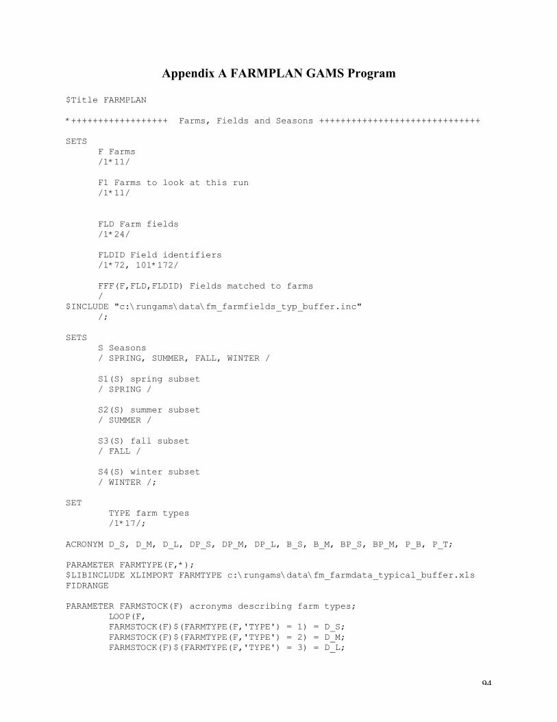
94
Appendix A FARMPLAN GAMS Program
$Title FARMPLAN
*++++++++++++++++++ Farms, Fields and Seasons ++++++++++++++++++++++++++++++
SETS F Farms /1*11/
F1 Farms to look at this run /1*11/
FLD Farm fields /1*24/
FLDID Field identifiers /1*72, 101*172/
FFF(F,FLD,FLDID) Fields matched to farms /$INCLUDE "c:\rungams\data\fm_farmfields_typ_buffer.inc" /;
SETS S Seasons / SPRING, SUMMER, FALL, WINTER /
S1(S) spring subset / SPRING /
S2(S) summer subset / SUMMER /
S3(S) fall subset / FALL /
S4(S) winter subset / WINTER /;
SET TYPE farm types /1*17/;
ACRONYM D_S, D_M, D_L, DP_S, DP_M, DP_L, B_S, B_M, BP_S, BP_M, P_B, P_T;
PARAMETER FARMTYPE(F,*);$LIBINCLUDE XLIMPORT FARMTYPE c:\rungams\data\fm_farmdata_typical_buffer.xlsFIDRANGE
PARAMETER FARMSTOCK(F) acronyms describing farm types; LOOP(F, FARMSTOCK(F)$(FARMTYPE(F,'TYPE') = 1) = D_S; FARMSTOCK(F)$(FARMTYPE(F,'TYPE') = 2) = D_M; FARMSTOCK(F)$(FARMTYPE(F,'TYPE') = 3) = D_L;

95
FARMSTOCK(F)$(FARMTYPE(F,'TYPE') = 4) = DP_S; FARMSTOCK(F)$(FARMTYPE(F,'TYPE') = 5) = DP_M; FARMSTOCK(F)$(FARMTYPE(F,'TYPE') = 6) = DP_L; FARMSTOCK(F)$(FARMTYPE(F,'TYPE') = 17) = B_S; FARMSTOCK(F)$(FARMTYPE(F,'TYPE') = 7) = B_M; FARMSTOCK(F)$(FARMTYPE(F,'TYPE') = 12) = BP_S; FARMSTOCK(F)$(FARMTYPE(F,'TYPE') = 13) = BP_M; FARMSTOCK(F)$(FARMTYPE(F,'TYPE') = 15) = P_B; FARMSTOCK(F)$(FARMTYPE(F,'TYPE') = 16) = P_T; );
*++++++++++++++++++ Crop Data +++++++++++++++++++++++++++++++++++++++++++++
SETS C Crops / BUFFEST buffer establishment red clover orchard grass BUFFER established buffer red clover orchard grass GRHAYEST establishment of red clover orchard grass for hay or pasture CG corn grain CS corn silage GRHAY red clover orchard grass hay maintenance RYESIL rye silage ALFEST alfalfa establishment ALFHAY established alfalfa hay PAST permanent pasture red clover orchard grass /
T Tillage methods /CONV conventional tillage NOTILL no-tillage row crop or hay establishment /
CT(C,T) acceptable tillage-crop combinations /(CS, CG, ALFEST, ALFHAY, GRHAYEST, GRHAY).(CONV, NOTILL), (RYESIL, BUFFEST,BUFFER).CONV, PAST.NOTILL /
CR Crop Rotations(all 1 acre per year soil resource use) / NTCG no-till corn grain CTCG conv-till corn grain NTCS no-till corn silage CTCS conv-till corn silage CTGRHAY conv-till grass hay establishment (0.143) and orch grass-clover pasture (0.857 acre) NTGRHAY no-till grass hay establishment (0.143) and orch grass-cloverpasture (0.857 acre) NTCSRYE no-till corn silage (1 acre)&Ryelage (1 acre) CTCSRYE conv-till corn silage (1 acre)&Ryelage (1 acre) NTCGRYE no-till corn grain (1 acre)&Ryelage (1 acre) CTCGRYE conv-till corn grain (1 acre)&Ryelage (1 acre) NTCSALF no-till corn silage(0.286 ac.)&Alf est(0.143ac.)&alfalfa(0.572 ac.) CTCSALF conv-till corn sil(0.286 ac.)&Alf est(0.143 ac.)&alfalfa(0.572ac.) NTCGALF no-till corn grain(0.286 acre)&Alf est(0.143ac.)&alfalfa(0.572 ac.)

96
CTCGALF conv-till corn gr(0.286 acre)&Alf est(0.143 ac.)&alfalfa(0.572ac.) PERMPAST no-till orch grass-clover establishment (0.143 ac.) & clover-orch grass pasture (0.857 acre) BUFFNAR Permanent buffer (1 acre) /
CRCT(CR,C,T) acceptable crop rotation-crop-tillage combinations / NTCS.CS.NOTILL, CTCS.CS.CONV, NTCG.CG.NOTILL, CTCG.CG.CONV, NTCSRYE.CS.NOTILL, NTCSRYE.RYESIL.CONV, CTCSRYE.CS.CONV, CTCSRYE.RYESIL.CONV, NTCGRYE.CG.NOTILL, NTCGRYE.RYESIL.CONV, CTCGRYE.CG.CONV, CTCGRYE.RYESIL.CONV, NTCSALF.CS.NOTILL, NTCSALF.ALFEST.NOTILL, NTCSALF.ALFHAY.NOTILL, CTCSALF.CS.CONV, CTCSALF.ALFEST.CONV, CTCSALF.ALFHAY.CONV, NTCGALF.CG.NOTILL, NTCGALF.ALFEST.NOTILL, NTCGALF.ALFHAY.NOTILL, CTCGALF.CG.CONV, CTCGALF.ALFEST.CONV, CTCGALF.ALFHAY.CONV, CTGRHAY.GRHAYEST.CONV, CTGRHAY.GRHAY.CONV, NTGRHAY.GRHAYEST.NOTILL, NTGRHAY.GRHAY.NOTILL, PERMPAST.GRHAYEST.NOTILL, PERMPAST.PAST.NOTILL, BUFFNAR.BUFFEST.CONV, BUFFNAR.BUFFER.CONV
/
PARAMETER YIELDS(FLDID,*) yields by field;$LIBINCLUDE XLIMPORT YIELDS c:\rungams\data\fm_farmdata_typical_buffer.xlsyieldrange
* grass hay yields are tall grass (orchard grass)-clover mix* alfalfa, corn grain, corn silage yields are no-till
PARAMETER MAXFLDF1(F,FLD,FLDID) field size ; LOOP (F, LOOP (FLD, LOOP (FLDID, MAXFLDF1(F,FLD,FLDID)$FFF(F,FLD,FLDID) = YIELDS(FLDID,'ACRES'); )));
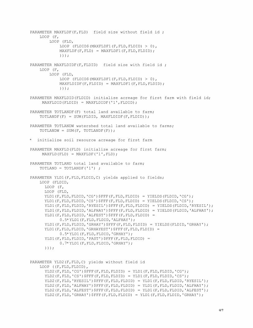
97
PARAMETER MAXFLDF(F,FLD) field size without field id ; LOOP (F, LOOP (FLD,
LOOP (FLDID$(MAXFLDF1(F,FLD,FLDID) > 0), MAXFLDF(F,FLD) = MAXFLDF1(F,FLD,FLDID); )));
PARAMETER MAXFLDIDF(F,FLDID) field size with field id ; LOOP (F, LOOP (FLD,
LOOP (FLDID$(MAXFLDF1(F,FLD,FLDID) > 0), MAXFLDIDF(F,FLDID) = MAXFLDF1(F,FLD,FLDID); )));
PARAMETER MAXFLDID(FLDID) initialize acreage for first farm with field id; MAXFLDID(FLDID) = MAXFLDIDF('1',FLDID);
PARAMETER TOTLANDF(F) total land available to farm; TOTLANDF(F) = SUM(FLDID, MAXFLDIDF(F,FLDID));
PARAMETER TOTLANDW watershed total land available to farms; TOTLANDW = SUM(F, TOTLANDF(F));
* initialize soil resource acreage for first farm
PARAMETER MAXFLD(FLD) initialize acreage for first farm; MAXFLD(FLD) = MAXFLDF('1',FLD);
PARAMETER TOTLAND total land available to farm; TOTLAND = TOTLANDF('1') ;
PARAMETER YLD1(F,FLD,FLDID,C) yields applied to fields; LOOP (FLDID,
LOOP (F, LOOP (FLD, YLD1(F,FLD,FLDID,'CG')$FFF(F,FLD,FLDID) = YIELDS(FLDID,'CG'); YLD1(F,FLD,FLDID,'CS')$FFF(F,FLD,FLDID) = YIELDS(FLDID,'CS');
YLD1(F,FLD,FLDID,'RYESIL')$FFF(F,FLD,FLDID) = YIELDS(FLDID,'RYESIL');YLD1(F,FLD,FLDID,'ALFHAY')$FFF(F,FLD,FLDID) = YIELDS(FLDID,'ALFHAY');YLD1(F,FLD,FLDID,'ALFEST')$FFF(F,FLD,FLDID) =
0.5*YLD1(F,FLD,FLDID,'ALFHAY');YLD1(F,FLD,FLDID,'GRHAY')$FFF(F,FLD,FLDID) = YIELDS(FLDID,'GRHAY');
YLD1(F,FLD,FLDID,'GRHAYEST')$FFF(F,FLD,FLDID) = 0.5*YLD1(F,FLD,FLDID,'GRHAY');
YLD1(F,FLD,FLDID,'PAST')$FFF(F,FLD,FLDID) = 0.7*YLD1(F,FLD,FLDID,'GRHAY');
)));
PARAMETER YLD2(F,FLD,C) yields without field id LOOP ((F,FLD,FLDID), YLD2(F,FLD,'CG')$FFF(F,FLD,FLDID) = YLD1(F,FLD,FLDID,'CG');
YLD2(F,FLD,'CS')$FFF(F,FLD,FLDID) = YLD1(F,FLD,FLDID,'CS');YLD2(F,FLD,'RYESIL')$FFF(F,FLD,FLDID) = YLD1(F,FLD,FLDID,'RYESIL');YLD2(F,FLD,'ALFHAY')$FFF(F,FLD,FLDID) = YLD1(F,FLD,FLDID,'ALFHAY');YLD2(F,FLD,'ALFEST')$FFF(F,FLD,FLDID) = YLD1(F,FLD,FLDID,'ALFEST');YLD2(F,FLD,'GRHAY')$FFF(F,FLD,FLDID) = YLD1(F,FLD,FLDID,'GRHAY');

98
YLD2(F,FLD,'GRHAYEST')$FFF(F,FLD,FLDID) = YLD1(F,FLD,FLDID,'GRHAYEST');YLD2(F,FLD,'PAST')$FFF(F,FLD,FLDID) = YLD1(F,FLD,FLDID,'PAST'););
* pasture yields = 70% grass hay yields (dry hay equiv) due to tramplingloss
PARAMETER YLD(F,FLD,C) harvested crop yields set to 0 for marginal soils toforce land into pasture; LOOP ((F,FLD),
YLD(F,FLD,C) = YLD2(F,FLD,C);YLD(F,FLD,'CG')$(YLD2(F,FLD,'CG') < 70) = 0;YLD(F,FLD,'CS')$(YLD2(F,FLD,'CS') < 11) = 0;YLD(F,FLD,'RYESIL')$(YLD2(F,FLD,'RYESIL') < 3) = 0;YLD(F,FLD,'ALFHAY')$(YLD2(F,FLD,'ALFHAY') < 3.5) = 0;YLD(F,FLD,'ALFEST')$(YLD2(F,FLD,'ALFEST') < 1.75) = 0;YLD(F,FLD,'GRHAY')$(YLD2(F,FLD,'GRHAY') < 2.5) = 0;YLD(F,FLD,'GRHAYEST')$(YLD2(F,FLD,'GRHAYEST') < 1.25) = 0;);
SET FCFLD(F,C,FLD) acceptable field crop combinations ; FCFLD(F,C,FLD) = YES$((YLD(F,FLD,C) GT 0.0)); FCFLD(F,"BUFFEST",FLD) = YES$((YLD(F,FLD,'PAST') GT 0.0)); FCFLD(F,"BUFFER",FLD) = YES$((YLD(F,FLD,'PAST') GT 0.0)); FCFLD(F,"GRHAYEST",FLD) = YES$((YLD(F,FLD,'GRHAY') GT 0.0)); FCFLD(F,"ALFEST",FLD) = YES$((YLD(F,FLD,'ALFHAY') GT 0.0));
SET CFLD(C,FLD) initialize acceptable field crop combinations for first farm; CFLD(C,FLD) = FCFLD('1',C,FLD);
SET FCTFLD(F,C,T,FLD) acceptable tillage-crop-field combinations ; FCTFLD(F,C,T,FLD) = CT(C,T) * FCFLD(F,C,FLD) ;
SET CTFLD(C,T,FLD) initialize acceptable tillage-crop-field combinations forfirst farm; CTFLD(C,T,FLD) = FCTFLD('1',C,T,FLD);
SET FCCRTFLD(F,C,CR,T,FLD) acceptable crop-crop rotation-field-tillagecombinations; FCCRTFLD(F,C,CR,T,FLD) = FCTFLD(F,C,T,FLD) * CRCT(CR,C,T);
SETS CP Crop products used for feed (bought or sold) /CORNG Corn Grain (bu) CORNS Corn Silage (ton) RYELG Ryelage (ton) ALFH Alfalfa hay (ton) GRHAYB Grass hay large bale (ton) SBOM soybean oil meal (ton) DICAL LIMESTONE OTHMINR /
CPP(CP) crop products that are produced on the farm / CORNG, CORNS, RYELG, ALFH, GRHAYB /

99
* CPL(CP) crop product that comes from broiler operation* /CBLITTER/
CSALE(CP) crop products that can be sold /CORNG, CORNS, ALFH, GRHAYB/
CBUY(CP) crop products that can be bought /CORNG, CORNS, ALFH, GRHAYB, SBOM, DICAL, LIMESTONE, OTHMINR /
PARAMETER FYLDS(F,FLD,CP,C) express crop yields as crop product yields ; FYLDS(F,FLD,"CORNS", "CS") = YLD(F,FLD,"CS"); FYLDS(F,FLD,"CORNG","CG") = YLD(F,FLD,"CG"); FYLDS(F,FLD,"RYELG","RYESIL") = YLD(F,FLD,"RYESIL"); FYLDS(F,FLD,"ALFH","ALFHAY") = YLD(F,FLD,"ALFHAY"); FYLDS(F,FLD,"ALFH","ALFEST") = YLD(F,FLD,"ALFEST"); FYLDS(F,FLD,"GRHAYB","GRHAY") = YLD(F,FLD,"GRHAY");
FYLDS(F,FLD,"GRHAYB","GRHAYEST") = YLD(F,FLD,"GRHAYEST"); FYLDS(F,FLD,"GRHAYB","PAST") = YLD(F,FLD,"PAST");
PARAMETER YLDS(FLD,CP,C) initialize crop yields as crop product yields forfirst farm; YLDS(FLD,CP,C) = FYLDS('1',FLD,CP,C);
PARAMETER ROTFRAC(CR,C,*) read in proportion of rotation acre in conv. ornotill;$LIBINCLUDE XLIMPORT ROTFRAC c:\rungams\data\FM_crop&live.xls rotation
PARAMETER ROTAC(CR,C,T) rotation ac fraction parameter with tillagedimension; ROTAC(CR, C, "CONV") = ROTFRAC(CR,C,"CONVFRAC") ; ROTAC(CR, C, "NOTILL") = ROTFRAC(CR,C,"NOTILLFRAC") ;
PARAMETER TVCACRE(C,T,*) prelim variable cost per acre (excl labor &nutrients);$LIBINCLUDE XLIMPORT TVCACRE c:\rungams\data\FM_crop&live.xls CRANGE
PARAMETER VCACRE(C,T) final variable cost per acre (excl labor & nutr); VCACRE(C,T)$CT(C,T) = TVCACRE(C,T,'VARCOST') ;* VCACRE('buffest',T) = BMPDATA('ANNOWNCS1','BUFFER') ;* VCACRE('buffer',T) = BMPDATA('ANNOWNCS1','BUFFER') ;
PARAMETER CROPPRIC(CP,*) crop product sell and buy prices ;$LIBINCLUDE XLIMPORT CROPPRIC c:\rungams\data\FM_crop&live.xls prange
PARAMETER CSP(CP) sale price of farm produced crop products ; CSP(CP) = CROPPRIC(CP,'CROPSALE') ;
PARAMETER CBUYP(CP) purchase price of crop products bought for feed ; CBUYP(CP) = CROPPRIC(CP,'CROPBUY') ;* grain assumed = sale price + $0.40/bu* hay assumed = sale price + $30/ton* SBOM taken from Virginia Farm Management Budgets
PARAMETER CROPLABOR(C,T,*) read in crop labor requirements by season ;$LIBINCLUDE XLIMPORT CROPLABOR c:\rungams\data\FM_crop&live.xls labrange* units = hours/acre

100
PARAMETER CROPLAB(C,T,S) convert crop labor to parameter with seasonal index; CROPLAB(C,T,"SPRING") = CROPLABOR(C,T,"SPRLABREQ") ; CROPLAB(C,T,"SUMMER") = CROPLABOR(C,T,"SUMLABREQ") ; CROPLAB(C,T,"FALL") = CROPLABOR(C,T,"FALLABREQ") ; CROPLAB(C,T,"WINTER") = CROPLABOR(C,T,"WTRLABREQ") ;
*++++++++++++++++++ Nutrient Data +++++++++++++++++++++++++++++++++++++++++*(Contains some livestock and manure data)
SETSNU nutrients used in crop production
/NITR nitrogen PHOS phosphate POTS potash /
R P2O5 application rates relative to minimum recommended levels / R1 * R8 /
NUMX(NU) nutrients subject to possible maximum restrictions from Prunoff /PHOS /
SETSNUTEST(NU) nutrients with soil test values for farm
/ PHOS, POTS /
NS fertilizer and manure nutrients sources for crops /DMAN 1000 gal liq dairy manure 6% dry matter BLIT ton broiler litter 72% dry matter TLIT ton turkey litter 65% dry matter COMNITR cwt ammonium nitrate 33% N COMPHOS cwt triple superphosphate 46% P2O5 COMPOTSH cwt muriate of potash 60% K2O /
LNS(NS) livestock manure nutrient sources / DMAN, BLIT, TLIT /
NSS(NS,S) acceptable seasons for spreading crop nutrient sources / (DMAN, BLIT, TLIT).(SPRING, SUMMER, FALL, WINTER), COMNITR.(SPRING, SUMMER, FALL), (COMPHOS, COMPOTSH).(SPRING, FALL) /
CNSS(C,NS,S) acceptable seasons for spreading crop nutrient sources oncrops / (PAST, BUFFEST, BUFFER).( DMAN, BLIT, TLIT).(SPRING, SUMMER, FALL,WINTER), (PAST, BUFFEST, BUFFER).(COMNITR, COMPHOS, COMPOTSH).(SPRING, SUMMER,FALL), (CS, CG, ALFEST, ALFHAY, GRHAYEST, GRHAY).( DMAN, BLIT, TLIT).(SPRING,FALL, WINTER), (CS, CG, ALFEST, ALFHAY, GRHAYEST, GRHAY).(COMPHOS, COMPOTSH).(SPRING,FALL), (CS, CG, ALFEST, ALFHAY, GRHAYEST, GRHAY).(COMNITR).(SPRING, SUMMER,FALL), RYESIL.( DMAN, BLIT, TLIT).( FALL, WINTER),

101
RYESIL.( COMPHOS, COMPOTSH). FALL, RYESIL.COMNITR.(FALL, SPRING) /
PARAMETER NUTRIENT(NS,*) costs and physical characteristics of nutrientsources ;$LIBINCLUDE XLIMPORT NUTRIENT c:\rungams\data\FM_crop&live.xls nutrange
PARAMETER NUTCONT(NS,NU) nutrient content of fertilizer or manure ; NUTCONT(NS,"NITR") = NUTRIENT(NS, "NCONT"); NUTCONT(NS,"PHOS") = NUTRIENT(NS, "P2O5CONT"); NUTCONT(NS,"POTS") = NUTRIENT(NS, "K2OCONT");* as removed from storage or feedlot just prior to application
PARAMETER NUTPRICE(NS,S) farm-delivered price of purchased crop nutr ;NUTPRICE(NS,"SPRING") = NUTRIENT(NS,"SPRFERTP") ;NUTPRICE(NS,"SUMMER") = NUTRIENT(NS,"SUMFERTP") ;NUTPRICE(NS,"FALL") = NUTRIENT(NS,"FALFERTP") ;NUTPRICE(NS,"WINTER") = NUTRIENT(NS,"WTRFERTP") ;
PARAMETER NAPPCST(NS) application cost per unit crop nutrient source ; NAPPCST(NS) = NUTRIENT(NS,"APPCOST") ;
SET FCTFLDNSS acceptable crop tillage field nutrient source & season comb ; FCTFLDNSS(F,C,T,FLD,NS,S) = CNSS(C,NS,S)* FCFLD(F,C,FLD) * CT(C,T) ;
SET CTFLDNSS initialize acceptable crop tillage field nutrient source &season comb ; CTFLDNSS(C,T,FLD,NS,S) = FCTFLDNSS('1',C,T,FLD,NS,S) ;
PARAMETER FNIT(F,C,FLD) recommended nitrogen application by field;* see Virginia Nutrient Management Standards and Criteria* cg 1 based on 1 lb/bu.* cs 7.5 based on 65 to 160 lbs for yield range of 10-21 tons* buffest = 40, buffer = 0 (assumed legume, red clover-orchard grassmix)* grhayest 40, legume (clover-orchard grass)* grhay 0, legume (clover-orchard grass)* ryesil 22 lbs/ton based on 100 lbs/ac all soil classes and assumed4.5 ton/ac yield* alfhay, alfest 0, legume* past 0, legume (red clover-orchard grass) FNIT(F,'CG',FLD) = YLD(F,FLD,"CG") ; FNIT(F,'CS',FLD) = YLD(F,FLD,"CS")*7.5; FNIT(F,'BUFFEST',FLD) = 40 ; FNIT(F,'BUFFER',FLD) = 0 ; FNIT(F,'GRHAYEST',FLD) = 40 ; FNIT(F,'GRHAY',FLD) = 0 ; FNIT(F,'RYESIL',FLD) = YLD(F,FLD,'RYESIL')*22; FNIT(F,'ALFEST',FLD) = 0 ; FNIT(F,'ALFHAY',FLD) = 0 ; FNIT(F,'PAST',FLD) = 0 ;
PARAMETER NIT(C,FLD) initialize recommended nitrogen application by field; NIT(C,FLD) = FNIT('1',C,FLD);
PARAMETER PMED1(F,C,FLD) recommended P2O5 application for soil testing mediumin P;

102
* see Virginia Nutrient Management Standards and Criteria* P2O5 per unit of yield based on following yield ranges and P2O5application recommendations* cg 0.5 lb/bu, 65 to 165 bu; 40-80 lbs* cs 4 lb/ton, 10 to 21 tons; 40-80 lbs* buffest, 130 lb/ac (assumed red clover-orchard grass mix)* buffer, 65 lb/ac (assumed red clover-orchard grass mix, average ofsoil productivity I,II,III and IV, constant applic. for all soils)* grhay, 20, 2.5 to 4 tons; 50-80 lbs (red clover-orchard grass)* grhayest, 130 (assumed red clover-orchard grass mix)* ryesil 20, 2 to 4.5 tons; 40-80 lbs* alfhay, 12.5, 3.5 to 6.5 tons, 50 to 80 lbs* alfest 130 (all soils)* past 20, 2.5 to 4 tons; 50-80 lbs (same as grass hay--red clover-orchard grass) PMED1(F,'CG',FLD) = YLD(F,FLD,'CG')*0.5; PMED1(F,'CS',FLD) = YLD(F,FLD,'CS')*4; PMED1(F,'BUFFEST',FLD) = 130; PMED1(F,'BUFFER',FLD) = 65; PMED1(F,'GRHAYEST',FLD) = 130; PMED1(F,'GRHAY',FLD) = YLD(F,FLD,'GRHAY')*20; PMED1(F,'RYESIL',FLD) = YLD(F,FLD,'RYESIL')*20; PMED1(F,'ALFEST',FLD) = 130; PMED1(F,'ALFHAY',FLD) = YLD(F,FLD,'ALFHAY')*12.5; PMED1(F,'PAST',FLD) = YLD(F,FLD,'PAST')*20;
PARAMETER PHI1(F,C,FLD) recommended P2O5 application for soil testing high inP;* see Virginia Nutrient Management Standards and Criteria* P2O5 per unit of yield based on following yield ranges and P2O5application recommendations* cg 0.25, 65 to 165 bu; 20-40 lbs* cs 2, 10 to 21 tons; 20-40 lbs* buffest, 75 (assumed red clover-orchard grass mix)* buffer 45 (assumed red clover-orchard grass mix soil average of soilproductivity I,II,III and IV, constant applic. for all soils)* grhay 12.5, 2.5 to 4 tons; 40-50 lbs (red clover-orchard grass)* grhayest, 75 (assumed red clover-orchard grass mix)* ryesil 10, 2 to 4.5 tons; 20-40 lbs* alfhay 8, 3.5 to 6.5 tons, 40 to 50 lbs* alfest 80 (all soils)* past 12.5, 2.5 to 4 tons; 40-50 lbs (same as grass hay--red clover-orchard grass) PHI1(F,'CG',FLD) = YLD(F,FLD,'CG')*0.25; PHI1(F,'CS',FLD) = YLD(F,FLD,'CS')*2; PHI1(F,'BUFFEST',FLD) = 75; PHI1(F,'BUFFER',FLD) = 45; PHI1(F,'GRHAYEST',FLD) = 75; PHI1(F,'GRHAY',FLD) = YLD(F,FLD,'GRHAY')*12.5; PHI1(F,'RYESIL',FLD) = YLD(F,FLD,'RYESIL')*10; PHI1(F,'ALFEST',FLD) = 80; PHI1(F,'ALFHAY',FLD) = YLD(F,FLD,'ALFHAY')*8; PHI1(F,'PAST',FLD) = YLD(F,FLD,'PAST')*12.5;
PARAMETER PVHI1(F,C,FLD) recommended P2O5 application for soil testing veryhigh in P; PVHI1(F,C,FLD) = 0.0;

103
PARAMETER KMED1(F,C,FLD) recommended K2O application for soil testing mediumin K;* see Virginia Nutrient Management Standards and Criteria* K2O per unit of yield based on following yield ranges and K2Oapplication recommendations* cg 0.5, 65 to 165 bu; 40-80 lbs* cs 8.0, 10 to 21 tons; 80-160 lbs* buffest, 130 (assumed red clover-orchard grass mix)* buffer 130 (assumed red clover-orchard grass mix, average of soilproductivity I,II,III and IV, constant applic. for all soils)* grhay 42.5, 2.5 to 4 tons; 95-170 lbs (red clover-orchard grass)* grhayest, 130 (assumed red clover-orchard grass mix)* ryesil 20, 2 to 4.5 tons; 40-80 lbs* alfest 130 (all soils)* alfhay 38.0, 3.5 to 6.5 tons, 170 to 245 lbs* past 42.5, 2.5 to 4 tons; 95-170 lbs (same as grass hay--red clover-orchard grass) KMED1(F,'CG',FLD) = YLD(F,FLD,'CG')*0.5; KMED1(F,'CS',FLD) = YLD(F,FLD,'CS')*8; KMED1(F,'BUFFEST',FLD) = 130; KMED1(F,'BUFFER',FLD) = 130; KMED1(F,'GRHAYEST',FLD) = 130; KMED1(F,'GRHAY',FLD) = YLD(F,FLD,'GRHAY')*42.5; KMED1(F,'RYESIL',FLD) = YLD(F,FLD,'RYESIL')*20; KMED1(F,'ALFEST',FLD) = 130; KMED1(F,'ALFHAY',FLD) = YLD(F,FLD,'ALFHAY')*38.0; KMED1(F,'PAST',FLD) = YLD(F,FLD,'PAST')*42.5;
PARAMETER KHI1(F,C,FLD) recommended K2O application for soil testing high inK;* see Virginia Nutrient Management Standards and Criteria* K2O per unit of yield based on following yield ranges and K2Oapplication recommendations* cg 0.25, 65 to 165 bu; 20-40 lbs* cs 4.0, 10 to 21 tons; 40-80 lbs* buffest, 75 (assumed red clover-orchard grass mix )* buffer 70 (assumed red clover-orchard grass mix, average of soilproductivity I,II,III and IV, constant applic. for all soils)* grhay 22.5, 2.5 to 4 tons; 55-90 lbs (red clover-orchard grass)* grhayest, 75 (assumed red clover-orchard grass mix)* ryesil 10, 2 to 4.5 tons; 20-40 lbs* alfest 80 (all soils)* alfhay 19.0, 3.5 to 6.5 tons, 90 to 120 lbs* past 22.5, 2.5 to 4 tons; 55-90 lbs (same as grass hay--red clover-orchard grass) KHI1(F,'CG',FLD) = YLD(F,FLD,'CG')*0.25; KHI1(F,'CS',FLD) = YLD(F,FLD,'CS')*4; KHI1(F,'BUFFEST',FLD) = 75; KHI1(F,'BUFFER',FLD) = 70; KHI1(F,'GRHAYEST',FLD) = 75; KHI1(F,'GRHAY',FLD) = YLD(F,FLD,'GRHAY')*22.5; KHI1(F,'RYESIL',FLD) = YLD(F,FLD,'RYESIL')*10; KHI1(F,'ALFEST',FLD) = 80; KHI1(F,'ALFHAY',FLD) = YLD(F,FLD,'ALFHAY')*19.0; KHI1(F,'PAST',FLD) = YLD(F,FLD,'PAST')*22.5;

104
PARAMETER KVHI1(F,C,FLD) recommended K2O application for soil testing veryhigh in K; KVHI1(F,C,FLD) = 0.0;
PARAMETER PREMOVCOEF(C) p2o5 removal per unit crop yield from Ches. BayRegion Nutrient Management Training Manual /BUFFEST 15, BUFFER 15, CG 0.4, CS 7.5, GRHAYEST 15, GRHAY 15, RYESIL5.6, ALFEST 11, ALFHAY 11, PAST 15/
PARAMETER PREMOVLF(F,C,FLD) estimated pounds of P2O5 removal per acre ofcrop;
PREMOVLF(F,C,FLD) = YLD(F,FLD,C)*PREMOVCOEF(C);
PARAMETER PREMOVL(C,FLD) initialize p2o5 removal per acre of crop; PREMOVL(C,FLD) = PREMOVLF('1',C,FLD);
PARAMETER MANNUF1(F,*) livestock manure capacity by farm ;$LIBINCLUDE XLIMPORT.GMS MANNUF1c:\rungams\data\fm_farmdata_typical_buffer.xls manurange
PARAMETER MANNUF(F,NU) livestock manure nutrient capacity by farm ; MANNUF(F,'PHOS') = MANNUF1(F,'MANP2O5'); MANNUF(F,'POTS') = MANNUF1(F,'MANK2O');
PARAMETER SOILTSTF(F,NU) estimate farm soil test levels for P and K ;* Jim Pease rule (4-15-2000) If potential manure nutrient/acre are 0-120then STP and STK are medium (=1),* if 120-180 then STP and STK are high (=2), if >180 then STP and STK arevery high (=3)
LOOP(F$(TOTLANDF(F) > 0), LOOP(NU$NUTEST(NU), IF(MANNUF(F,NU)/TOTLANDF(F) > 180, SOILTSTF(F,NU) = 3; ELSEIF(MANNUF(F,NU)/TOTLANDF(F) < 180) AND(MANNUF(F,NU)/TOTLANDF(F) > 120), SOILTSTF(F,NU) = 2; ELSE SOILTSTF(F,NU) = 1); ));* SOILTSTF('2',NU) = 3;
DISPLAY 'SOILTSTF HERE', SOILTSTF;* initialize farm soil testPARAMETER SOILTST(NU) farm soil test for P and K ; SOILTST(NU)$NUTEST(NU) = SOILTSTF('1',NU) ;
PARAMETER MINRECF(F,C,FLD,NU) farm minimum recommended nutrient applications; LOOP (F, MINRECF(F,C,FLD,"NITR") = FNIT(F,C,FLD) ; IF (SOILTSTF(F,"PHOS") = 1, MINRECF(F,C,FLD,"PHOS") = PMED1(F,C,FLD) ; ELSEIF SOILTSTF(F,"PHOS") = 2, MINRECF (F,C,FLD,"PHOS") = PHI1(F,C,FLD) ; ELSE

105
MINRECF(F,C,FLD,"PHOS") = PVHI1(F,C,FLD)) ; IF (SOILTSTF(F,"POTS") = 1, MINRECF (F,C,FLD,"POTS") = KMED1(F,C,FLD) ; ELSEIF SOILTSTF(F,"POTS") = 2,
MINRECF (F,C,FLD,"POTS") = KHI1(F,C,FLD) ; ELSE MINRECF (F,C,FLD,"POTS") = KVHI1(F,C,FLD)) ; );
DISPLAY 'MINRECF HERE', MINRECF;
PARAMETER MINREC initialized value of minimum recommended phosphate applic; MINREC (C,FLD,NU) = MINRECF('1',C,FLD,NU) ;
*The following application parameters are not used in this study, JB
PARAMETER RATE(R) p2o5 application rate relative to recommended or cropremoval levels /R1 1, R2 1.25, R3 1.5, R4 1.75, R5 2, R6 3, R7 4, R8 20 /
PARAMETER NUTAPRATF(F,C,FLD,R) p205 application rates per acre; NUTAPRATF(F,C,FLD,R) =RATE(R)*(MINRECF(F,C,FLD,"PHOS")$(MINRECF(F,C,FLD,"PHOS") GTPREMOVLF(F,C,FLD)) + PREMOVLF(F,C,FLD)$(MINRECF(F,C,FLD,"PHOS")LE PREMOVLF(F,C,FLD))); NUTAPRATF(F,C,FLD,'R1') = RATE('R1')*(MINRECF(F,C,FLD,"PHOS"));* application rates greater than 1 allow getting rid of manure byoverapplying relative to recommended or P removal* whichever is larger* minimum application rate equal to 1 is based on applying p2o5 atrecommended level
* set rate for highest applic at 200 if would otherwise be 0 such as forhay establishment on soils very high in p2o5 LOOP (F, LOOP (C, LOOP (FLD, IF ((NUTAPRATF(F,C,FLD,'R8') = 0), NUTAPRATF(F,C,FLD,'R8') = 200))));
PARAMETER NUTAPRAT(C,FLD,R) initialize p2o5 application rate for first farm; NUTAPRAT(C,FLD,R) = NUTAPRATF('1',C,FLD,R);
PARAMETER EXCESSP(F,C,FLD,R) p2o5 applied that exceeds the minimumrecommended phosphate application; EXCESSP(F,C,FLD,R) = NUTAPRATF(F,C,FLD,R) -MINRECF(F,C,FLD,'PHOS');
PARAMETER ORGNPCT(NS) organic N as percent of total N in fert source ; ORGNPCT(NS) = NUTRIENT(NS, "ORGN");
PARAMETER ORGNCONT(NS) organic N content in fert source ; ORGNCONT(NS) = (ORGNPCT(NS)/100)*NUTCONT(NS,"NITR");

106
PARAMETER ONAVL(NS) percent of organic N which becomes crop available; ONAVL(NS) = NUTRIENT(NS, "ONAVAIL");
PARAMETER AVONCONT(NS) available organic N contained in nutrient source; AVONCONT(NS) = (ONAVL(NS)/100) * ORGNCONT(NS);
PARAMETER NVOLAT(NS) pct of inorganic N volatilized prior to crop uptake; NVOLAT(NS) = NUTRIENT(NS, "NVOL");
PARAMETER AVINCONT(NS) avail & utilizable inorg N in nutrient source; AVINCONT(NS) = (NUTCONT(NS,"NITR") - ORGNCONT(NS))*(1 -(NVOLAT(NS)/100));
PARAMETER NUTCONT1(NS, NU) plant available nutr in fertilizer & manure; NUTCONT1(NS, "NITR") = AVINCONT(NS) + AVONCONT(NS); NUTCONT1(NS, "PHOS") = NUTCONT(NS, "PHOS"); NUTCONT1(NS, "POTS") = NUTCONT(NS, "POTS");
*++++++++++++++++++ Livestock Data +++++++++++++++++++++++++++++++++++++++++
SETSL livestock
/DAIRY 1 lactating dairy cow (fed 305 days) 1 dry cow (fed 60 days) &0.9 repl hfrs STOCKER 1 stocker steer (fall to fall 450 to 925 lbs) BEEFCOW 1 beef cow&0.15 repl. heifer&0.9 calf&0.1 bull BROILER 1 house cap. 25K birds 6.4 cycles year TURKEY 1 house cap. toms 16K birds 4 cycles year/
B(L) beef livestock /STOCKER, BEEFCOW /
SET NB(L) non-beef livestock ; NB(L) = NOT B(L) ;
SETSLP livestock products for sale or use on farm
/MILK cwt milk from dairy STOCKSEL cwt stocker BEEFCALF cwt weaned beef calf BROILSEL annual output from 1 broiler house (160000 birds) TURKSEL annual output from turkey house (64000 birds)/
LMP livestock recoverable manure production /DAIRYMAN 1000 gallons dairy liquid 6 pct dry matter PBLITTER tons broiler litter 72 pct dry matter TURKLIT tons turkey litter 65 pct dry matter /
LLMP(L,LMP) acceptable livestock-manure combinations / DAIRY.DAIRYMAN, BROILER.PBLITTER, TURKEY.TURKLIT /
LMPF(LMP) manure that can be used as feed / PBLITTER /
FR Livestock & poultry feed rations
107
/
DAIRYALF Milk cow alfalfa ration incl dry cow & repl heifer DAIRYCS milk cow corn silage ration incl dry cow & repl heifer DAIRYRYE milk cow ryelage ration incl dry cow & repl heifer STKRHAY stocker ration hay pasture broiler litter & corn BFCOWHAY beef cow hay pasture & broiler litter BRR1 Broiler ration TUR1 Turkey ration /
LFR(L, FR) Ration by livestock type /DAIRY.(DAIRYALF,DAIRYCS,DAIRYRYE), STOCKER.STKRHAY,BEEFCOW.BFCOWHAY,
BROILER.BRR1,TURKEY.TUR1/;
PARAMETER MAXLIVE(F,*) livestock capacity by farm ;$LIBINCLUDE XLIMPORT.GMS MAXLIVEc:\rungams\data\fm_farmdata_typical_buffer.xls livrange
PARAMETER MAXLIVF(F,L) maximum livestock capacity of farm facilities ; MAXLIVF(F,'DAIRY') = MAXLIVE(F,'DAIRY'); MAXLIVF(F,'BEEFCOW') = MAXLIVE(F,'BEEFCOW'); MAXLIVF(F,'BROILER') = MAXLIVE(F,'BROILER'); MAXLIVF(F,'TURKEY') = MAXLIVE(F,'TURKEY');
PARAMETER MAXLIVW(L) watershed livestock capacity of farm facilities ; MAXLIVW(L) = SUM(F, MAXLIVF(F,L)) ;
* initialize livestock capacity
PARAMETER MAXLIV(L) farm livestock capacity; MAXLIV(L) = MAXLIVF('1',L) ;
PARAMETER LIVESTOK(L,*) livestock yield and costs ;$LIBINCLUDE XLIMPORT LIVESTOK c:\rungams\data\FM_crop&live.xls liverange
PARAMETER LYIELD(L,LP) annual yield of livestock product per unit oflivestock;* units milk = cwt, stocksel = cwt stocker, beefcow = cwt calf,* broilsel = 1,000 broilers, turksel = 1,000 turkey toms
LYIELD("DAIRY","MILK") = LIVESTOK('DAIRY','LIVYIELD') ; LYIELD("STOCKER","STOCKSEL") = LIVESTOK('STOCKER','LIVYIELD') ; LYIELD("BEEFCOW","BEEFCALF") = LIVESTOK('BEEFCOW','LIVYIELD') ; LYIELD("BROILER","BROILSEL") = LIVESTOK('BROILER','LIVYIELD') ; LYIELD("TURKEY","TURKSEL") = LIVESTOK('TURKEY','LIVYIELD') ;
PARAMETER LPRICE(LP) sale price of livestock products ;* milk, stockers, and beef calves are $/cwt* broilers & turkeys are contract fees per 1000 birds
LPRICE('MILK') = LIVESTOK('DAIRY','SELPRICE') ; LPRICE('STOCKSEL') = LIVESTOK('STOCKER','SELPRICE') ; LPRICE('BEEFCALF') = LIVESTOK('BEEFCOW','SELPRICE') ; LPRICE('BROILSEL') = LIVESTOK('BROILER','SELPRICE') ; LPRICE('TURKSEL') = LIVESTOK('TURKEY','SELPRICE') ;

108
PARAMETER MLIVEINC(L) miscellaneous livestock income culls etc ;
MLIVEINC(L) = LIVESTOK(L,'MISCINCO');
PARAMETER LCOST(L) livestock variable cost (excl labor & feed) ;
LCOST(L) = LIVESTOK(L,'LIVCOST');
PARAMETER LMPROD(L,LMP) annual recoverable manure prodn per unit livestock;* DAIRYMAN = 1000 gallons dairy liquid 6 pct dry matter* PBLITTER = tons broiler litter 72 pct dry matter* TURKLIT = tons turkey litter 65 pct dry matter
LMPROD('DAIRY','DAIRYMAN') = LIVESTOK('DAIRY','MANUPROD'); LMPROD('BROILER','PBLITTER') = LIVESTOK('BROILER','MANUPROD'); LMPROD('TURKEY','TURKLIT') = LIVESTOK('TURKEY','MANUPROD');
PARAMETER LMPRODS(L,S,LMP) seasonal recoverable manure prodn ;LMPRODS(L,S,LMP) = LMPROD(L,LMP)/4 ;
PARAMETER LIVELAB(L,S) livestock labor requirement per season ;* hours per unit of livestock enterprise LIVELAB(L,'SPRING') = LIVESTOK(L,'LIVLABSPR') ; LIVELAB(L,'SUMMER') = LIVESTOK(L,'LIVLABSUM') ; LIVELAB(L,'FALL') = LIVESTOK(L,'LIVLABFAL') ; LIVELAB(L,'WINTER') = LIVESTOK(L,'LIVLABWTR') ;
PARAMETER LLABYR(L) livestock labor requirement per year; LLABYR(L) = SUM(S, LIVELAB(L,S));
PARAMETER FRCONT(CP,FR) feed inputs to rations ;
$LIBINCLUDE XLIMPORT FRCONT c:\rungams\data\FM_crop&live.xls ratrange
*++++++++++++++++++ Manure Data ++++++++++++++++++++++++++++++++++++++++++++
PARAMETER MANURE(LMP, *) manure related parameters ;$LIBINCLUDE XLIMPORT MANURE c:\rungams\data\FM_crop&live.xls manrange
PARAMETER MANSPRIC(LMP,S) seasonal sale price of manure at farmgate;MANSPRIC(LMP,"SPRING") = MANURE(LMP, "SPRPRIC") ;MANSPRIC(LMP,"SUMMER") = MANURE(LMP, "SUMPRIC") ;MANSPRIC(LMP,"FALL") = MANURE(LMP, "FALPRIC") ;MANSPRIC(LMP,"WINTER") = MANURE(LMP, "WTRPRIC") ;
TABLE MANCONVRT(NS,LMP) create crop nutrient source from manure DAIRYMAN PBLITTER TURKLIT DMAN 1 0 0 BLIT 0 1 0 TLIT 0 0 1 ;
PARAMETER MSTOF(F,*) read in existing manure storage capacity in months;$LIBINCLUDE XLIMPORT MSTOF c:\rungams\data\fm_farmdata_typical_buffer.xlsstorange

109
PARAMETER MSTOCAPF(F,LMP) existing manure storage capacity ;* units: DAIRYMAN = 1000 gallons dairy liquid 6 pct dry matter* PBLITTER = tons broiler litter 72 pct dry matter* TURKLIT = tons turkey litter 65 pct dry matter MSTOCAPF(F,'DAIRYMAN') = MSTOF(F,'DMANSTORE') * MAXLIVF(F,'DAIRY') *(LMPROD('DAIRY','DAIRYMAN')/12); MSTOCAPF(F,'PBLITTER') = MSTOF(F,'BLITSTORE') * MAXLIVF(F,'BROILER') *(LMPROD('BROILER','PBLITTER')/12); MSTOCAPF(F,'TURKLIT') = MSTOF(F,'TLITSTORE') * MAXLIVF(F,'TURKEY') *(LMPROD('TURKEY','TURKLIT')/12);
PARAMETER MSTOCAPW(LMP) watershed manure storage capacity; MSTOCAPW(LMP) = SUM(F, MSTOCAPF(F, LMP)) ;
* initialize manure storage
PARAMETER MSTOCAP(LMP) existing manure storage capacity ; MSTOCAP(LMP) = MSTOCAPF('1',LMP) ;
PARAMETER STOCST(LMP) annualized cost of manure storage constr ;* cost to store manure for 6 mos.* includes deprec, interest, ins, repair, & tax
STOCST(LMP) = MANURE(LMP, "STORCOST") ;
*++++++++++++++++++ BMP Data ++++++++++++++++++++++++++++++++++++++++++++++
SETSBMP bmps incl buffers manure storage & nutr mgmt
/ MSTORE, NMP, BUFFER /
BMPATTRIB attributes of bmps
/INITCOST1 'initial per unit investment cost 1st type of each bmp, man.storage = dairy manure' INITCOST2 'initial per unit investment cost 2nd type of each bmp, man.storage = poultry litter' ANNOWNCS1 'annual ownership cost 1st type of each bmp, man. storage =dairy manure' ANNOWNCS2 'annual ownership cost 2nd type of each bmp, man. storage =poultry litter' LIFE 'economic life of bmp investment' INTRATE 'interest rate applied to bmp investment' MAINTPCT 'annual bmp maintenance cost as percent of initialinvestment' MINWIDTH 'minimum required width of buffer along blue line streams' MAXWIDTH 'maximum buffer width for which cost share and/or subsidy isavailable' NUTSTD 'standard applied to nutrient management plan (0 = none, 1 =nitrogen base, or 2 = phosphorus base)' MOSCAP 'months capacity of manure storage required on farm' SUBCOST 'annual subsidy per acre of nmp or buffer or per $1000 manurestorage investment' CSPCT 'percent of initial bmp investment cost shared by govt' ANNCS1 'annualized public cost share expense per unit of type 1 bmpadopted within each bmp class' ANNCS2 'annualized public cost share expense per unit of type 2 bmpadopted within each bmp class'

110
TECHCOST 'technical assistance cost per farm per bmp' ANNTECHCS 'annualized technical assistance cost per farm per bmp' INFOCOST 'cost per farm per bmp to inform farmers about bmp policy' ANNINFOCS 'annualized information cost per farm per bmp' CONTRCOST 'cost per farm per bmp to contract with farmers for bmpadoption' ANNCONTRCS 'annualized contracting cost per farm per bmp' ENFORCOST 'cost per farm per bmp to enforce bmp adoption' ANNENFCS 'annualized enforcement cost per farm per bmp'/
BMPIN(BMPATTRIB) attributes of bmps read from input file/INITCOST1 'initial per unit investment cost 1st type of each bmp, man.
storage = dairy manure' INITCOST2 'initial per unit investment cost 2nd type of each bmp, man.storage = poultry litter' ANNOWNCS1 'annual ownership cost 1st type of each bmp, man. storage =dairy manure' ANNOWNCS2 'annual ownership cost 2nd type of each bmp, man. storage =poultry litter' MINWIDTH 'minimum required width of buffer along blue line streams' MAXWIDTH 'maximum buffer width for which cost share and/or subsidy isavailable' NUTSTD 'standard applied to nutrient management plan (0 = none, 1 =nitrogen base, or 2 = phosphorus base)' MOSCAP 'months capacity of manure storage required on farm' SUBCOST 'annual subsidy per acre of nmp or buffer or per $1000 manurestorage investment' ANNCS1 'annualized public cost share expense per unit of type 1 bmpadopted within each bmp class' ANNCS2 'annualized public cost share expense per unit of type 2 bmpadopted within each bmp class' ANNTECHCS 'annualized technical assistance cost per farm per bmp' ANNINFOCS 'annualized information cost per farm per bmp' ANNCONTRCS 'annualized contracting cost per farm per bmp' ANNENFCS 'annualized enforcement cost per farm per bmp'/
TABLE BMPDATA(BMPIN, BMP) bmp attributes under this policy run
$INCLUDE "c:\rungams\data\FM_bmpdata2.inc";
PARAMETER NUTSTAND nutrient management standard applicable to farm ;NUTSTAND = BMPDATA('NUTSTD', 'NMP') ;
PARAMETER NMPREQ proportion of crop and pasture acres under mandatorynutrient management planning IF((NUTSTAND GT 0), NMPREQ = 1; ELSE NMPREQ = 0);
PARAMETER NSTOCST(LMP) net farmer annual ownership cost per ton or 1000 galof manure storage construction ;* includes deprec, interest on farmer share of const cost plus maintenance NSTOCST('DAIRYMAN') = MANURE('DAIRYMAN', 'STORCOST'); NSTOCST('PBLITTER') = MANURE('PBLITTER', 'STORCOST'); NSTOCST('TURKLIT') = MANURE('TURKLIT', 'STORCOST');

111
PARAMETER BLUE(F,FLD,*) read in acres of mandatory buffer ;$LIBINCLUDE XLIMPORT BLUE c:\rungams\data\fm_farmdata_typical_buffer.xlsbluebyfarm
PARAMETER BLUELINE(F,FLD) acres of field required to buffer adjacent streams; BLUELINE(F,FLD) = BLUE(F,FLD,'BUFFACRES');
PARAMETER BUFFMIN minimum buffer acres required on field ; BUFFMIN = BMPDATA('MINWIDTH', 'BUFFER') ;
PARAMETER BUFMNACF(F,FLD) minimum acres of buffer required on field ; BUFMNACF(F,FLD) = (BLUELINE(F,FLD) * BUFFMIN);
* initialize buffer minimumPARAMETER BUFMNAC farm minimum required buffer; BUFMNAC(FLD) = BUFMNACF('1',FLD) ;
*++++++++++++++++++ Labor Data ++++++++++++++++++++++++++++++++++++++++++++
* farm labor availability* assume that farm has available 3 hours labor per acre of cropland (approx.equal to* corn silage labor requirement) plus labor required per unit of livestocktimes livestock cap.
PARAMETER AVLABYRF(F) annual hours of labor available ; AVLABYRF(F) = SUM (L, (MAXLIVF(F,L) * LLABYR(L))) + (3.0 * SUM(FLD,MAXFLDF(F,FLD)));
* increase spring and fall labor availability and reduce summer and winterlabor availability* to reflect assumption that farmer works longer hours during planting andharvest
PARAMETER AVLABORF(F,S) hours of full-time labor available per season; AVLABORF(F,'WINTER') = 0.9*(AVLABYRF(F)/4); AVLABORF(F,'SPRING') = 1.1*(AVLABYRF(F)/4); AVLABORF(F,'SUMMER') = 0.9*(AVLABYRF(F)/4); AVLABORF(F,'FALL') = 1.1*(AVLABYRF(F)/4);
* initialize available labor
PARAMETER AVLABOR(S) ; AVLABOR(S) = AVLABORF('1',S) ;
PARAMETER LABPRICE cost per hour of part-time labor ;$LIBINCLUDE XLIMPORT LABPRICE c:\rungams\data\FM_crop&live.xls lcrange
*++++++++++++++++++ Crop and Nutrient Variables +++++++++++++++++++++++++++
VARIABLES
ALFTOT total acres of alfalfa incl establishmentALFTOTF(F) farm F total acres of alfalfa incl establishmentALFTOTW watershed total acres of alfalfa incl establishmentCNUTREQ(C,T,FLD,NU) recommended nutrient applic for crop and field

112
CNUTREQF(F,C,T,FLD,NU) recommended nutrient applic for crop and field andfarmCPROD(CP) total production of crop productCPRODF(F,CP) farm F total production of crop productCPRODW(CP) watershed total production of crop productCROPAC(C,T) acres of crop grown by tillage typeCROPACF(F,C,T) farm F acres of crop grown by tillage typeCROPACT(C) total acres of each crop grown on farm with all tillage typesCROPACTF(F,C) farm F acres of crop grownCROPACTW(C) watershed acres of crop grownCROPACFD(C,T,FLD) acres of crop grown by tillage type and fieldCROPACFDF(F,C,T,FLD) acres of crop grown by tillage type and fieldCROPACFDR(C,T,FLD,R) acres of crop grown by tillage type and field and papplication rateCRPACFDRF(F,C,T,FLD,R) farm F acres of crop grown by tillage type and fieldand p application rateCROPROTN(CR,FLD) acres of crop rotation grown by fieldCROPREV(CP) total revenues from sales of each cropCROPRVF(F,CP) farm F total revenues from sales of each cropCROPRVW(CP) watershed total revenues from sales of each cropCROPSELL(CP) total sales of each cropCROPSELF(F,CP) farm F total sales of each cropCROPSELW(CP) watershed total sales of each cropCROPVC(C) variable cost of each crop (excl labor and nutrients)CROPVCF(F,C) farm F variable cost of each crop (excl labor and nutrients)CROPVCW (C) watershed variable cost of each crop (excl labor and nutrients)CROTTOT(CR) total acres of crop rotation grown on farmCROTTOTF(F,CR) farm F total acres of crop rotation grown on farmCROTTOTW(CR) watershed total acres of crop rotation grown on farmCRPROTNF(F,CR,FLD) farm F acres of crop rotation grown by fieldFFLDAP(F,FLD) P2O5 application of field with farm idFFLDRP(F,FLD) P2O5 removal of field with farm idFLDAP(FLD) P2O5 application of fieldFLDRP(FLD) P2O5 removal of fieldGHAYTOT total acres of grass hay incl establishmentGHAYTOTF(F) farm F total acres of grass hay incl establishmentGHAYTOTW watershed total acres of grass hay incl establishmentCNUTBUY(C,NS,S) seasonal purchase of crop nutrient source per crop(fertilizer or manure)NUTBUY(NS,S) seasonal purchase of crop nutrient source (fertilizer or manure)NUTCST(NS) expenditures for purchased crop nutrient sourcesNUTCSTF(F,NS) farm F expenditures for purchased crop nutrient sourcesNUTCSTW(NS) watershed expenditures for purchased crop nutrient sourcesNUTSPRED(NS,S) total spreading crop nutrients (fertilizer or manure) byseasonNUTSPRDS(C,T,FLD,NS,S) seasonal spreading nutrient source on crop & FLDNUTSPDSF(F,C,T,FLD,NS,S) farm F seasonal spreading nutrient source on crop &FLDNUTSPDRF(F,C,T,FLD,NS,S) farm F seasonal spreading nutrient source rate peracre on crop & FLDTALFVC total alfalfa variable cost incl establishmentTALFVCF(F) farm F total alfalfa variable cost incl establishmentTALFVCW watershed total farm alfalfa variable cost incl establishmentTAPPCST total cost of spreading crop nutrientsTAPPCSTF(F) farm F total cost of spreading crop nutrientsTAPPCSTW watershed total cost of spreading crop nutrientsTCROPAP(NU) total nutrients applied on farm from all sources
113
TCROPAPF(F,NU) total nutrients applied on farm F from all sourcesTCROPAPW(NU) total nutrients applied in watershed from all sourcesTCROPPR total P2O5 removal by crops on the farmTCROPPRF total P2O5 removal by crops on farm FTCROPPRW total P2O5 removal by crops in watershedTCROPREC(NU) total recommended crop nutrient applications on farmTCROPRCF(F,NU) total recommended crop nutrient applications on farm FTCROPRCW(NU) total recommended crop nutrient applications on all farms inwatershedTCROPREV total revenues from all crop salesTCROPRVF(F) farm F total revenues from all crop salesTCROPRVW watershed total revenues from all crop salesTCROPVC total variable costs of crop production (excl nut & labor)TCROPVCF(F) farm F total variable costs of crop production (excl nut & labor)TCROPVCW watershed total variable costs of crop production (excl nut & labor)TGHVC total grass hay variable cost incl establishmentTGHVCF(F) farm F total grass hay variable cost incl establishmentTGHVCW watershed total grass hay variable cost incl establishmentTILLAGE(T) acres of crops grown under each tillage typeTILLAGEF(F,T) farm F acres of crops grown under each tillage typeTILLAGEW(T) watershed acres of crops grown under each tillage typeTNUTBUY(NS) total purchases of each type fertilizer or manureTNUTBUYF(F,NS) total farm F purchases of each type fertilizer or manureTNUTBUYW(NS) watershed total purchases of each type fertilizer or manureTNUTCST total expenditures for purchased crop nutrient sourcesTNUTCSTF(F) farm F total expenditures for purchased crop nutrient sourcesTNUTCSTW watershed total expenditures for purchased crop nutrient sourcesTNUTSPD(NS) total annual spreading crop nutrients (fertilizer or manure)TNUTSPDF(F,NS) farm F total annual spreading crop nutrients (fertilizer ormanure)TNUTSPDW(NS) watershed total annual spreading crop nutrients (fertilizer ormanure);*++++++++++++++++++ Livestock and Manure Variables ++++++++++++++++++++++++
VARIABLES
FACNBQF(F,L) shadow price on non-beef livestock facilities limit by farmFACBQF(F,L) shadow price on beef livestock facilities limit by farmFBUYCSTF(F,CP) farm F expenditures on each purchased livestock feed typeFBUYCSTW(CP) watershed expenditures on each purchased livestock feed typeFDBUYCST(CP) expenditures on each purchased livestock feed typeFEEDBUY(CP) feeds boughtFEEDBUYF(F,CP) farm F feeds boughtFEEDBUYW(CP) watershed feeds boughtFEEDFED(CP) feed fed to meet livestock feed requirementFEEDFEDF(F,CP) farm F feed fed to meet livestock feed requirementFEEDFEDW(CP) watershed feed fed to meet livestock feed requirementFNUTPRD(NS,S) farm produced manure by season used for crop applicationLIVEST(L,FR) number livestock produced by feed ration typeLIVEVC(L) variable cost of livestock production (excl feed & labor)LIVEVCF(F,L) farm F variable cost of livestock production (excl feed & labor)LIVEVCW(L) watershed variable cost of livestock production (excl feed &labor)LPREV(LP) revenue from sale of each livestock productLPREVF(F,LP) farm F revenue from sale of each livestock productLPREVW(LP) watershed revenue from sale of each livestock product

114
LPROD(LP) quantity of livestock products produced on farmLPRODF(F,LP) farm F quantity of livestock products produced on farmLPRODW(LP) watershed quantity of livestock products produced on farmLPSALES(LP) quantities of livestock products sold by farmLPSALESF(F,LP) farm F quantities of livestock products sold by farmLPSALESW(LP) watershed quantities of livestock products sold by farmsMANCONS(LMP,S) seasonal manure transfer to nutr source for cropMANFEEDS(LMP,S) convert farm produced litter to animal feedMANREV(LMP) revenues from sale of each manure typeMANREVF(F,LMP) farm F revenues from sale of each manure typeMANREVW(LMP) watershed revenues from sale of each manure typeMANSALS(LMP,S) seasonal sales of recoverable manure produced on farmMANSALSF(F,LMP,S) farm F seasonal sales of recoverable manure produced onfarmMANSALSW(LMP,S) watershed seasonal sales of recoverable manure produced onfarmMANSTOQF(F,S,LMP) shadow price on manure storage by livestock type and seasonMANSTOS(S,LMP) seasonal manure storageMPRODS(S,LMP) seasonal farm production of recoverable manureMPRODYR(LMP) annual farm production of recoverable manureMPRODYRF(F,LMP) farm F annual production of recoverable manureMPRODYRW(LMP) watershed annual production of recoverable manureTFEEDCST total cost of purchased feedTFDCSTF(F) farm F total cost of purchased feedTFDCSTW watershed total cost of purchased feedTLIVEST(L) total production of livestock of each typeTLIVESTF(F,L) farm F total livestock production of each typeTLIVESTW(L) watershed total livestock production of each typeTLIVEVC total variable cost of livestock (excl feed & labor)TLIVEVCF(F) total variable cost of livestock (excl feed & labor)TLIVEVCW watershed total variable cost of livestock (excl feed & labor)TMANCON(LMP) total manure conversion to crop nutrient sourceTMANFEED(LMP) total manure used for livestock feedTMANREV total revenues from manure sales on farmTMANREVF(F) farm F total revenues from manure sales on farmTMANREVW watershed total revenues from manure sales on farmTMANSAL(LMP) total annual sales of manure typeTMANSALF(F,LMP) farm F total annual sales of manure typeTMANSALW(LMP) watershed total annual sales of manure type
TRVLSTK total revenue from livestock product sales on farmTRVLSTKF(F) farm F total revenue from livestock product sales on farmTRVLSTKW watershed total revenue from livestock product sales on farm;*++++++++++++++++++ BMP Variables +++++++++++++++++++++++++++++++++++++++++
VARIABLES
BLDSTO(LMP) construction of a ton or 1000 gal of annual manure storageBLDSTOF(F,LMP) farm F construction of a ton or 1000 gal of annual manurestorageBLDSTOW(LMP) watershed construction of annual manure storageSUBREV farm revenue from subsidiesSUBREVF(F) farm F bmp subsidy revenueSUBREVW watershed total farm bmp subsidy revenueTBUFFVC total buffer variable cost incl establishmentTBUFFVCF(F) farm F total buffer variable cost incl establishment

115
TBUFFVCW watershed total buffer variable cost incl establishmentTNMPAC total acres covered by nutrient management planTNMPACF(F) farm F total acres covered by nutrient management planTNMPACW total watershed acres covered by nutrient management planTNMPCST farmers total annualized cost of nutrient management plan writingTNMPCSTF(F) farm F total annualized cost of nutrient management plan writingTNMPCSTW total watershed cost of nutrient management plan writingTSTOCST total annualized cost of building new manure storageTSTOCSTF(F) farm F total annualized cost of building new manure storageTSTOCSTW watershed total annualized cost of building new manure storage;*++++++++++++++++++ Other Variables +++++++++++++++++++++++++++++++++++++++
VARIABLES
HPTLAB(S) hired part-time labor by seasonLABUSE(S) total hours labor used in each seasonLABUSEF(F,S) farm F total hours labor used in each seasonLABUSEW(S) watershed total hours labor used in each seasonLANDQF(F,FLD) shadow price on land by FLDMODSTATF(F) model status for farm fPTLBCST(S) seasonal expenditure on part-time laborPTLBCSTF(F,S) farm F seasonal expenditure on part-time laborPTLBCSTW(S) watershed seasonal expenditure on part-time laborTCOST farm total variable costsTCOSTF(F) farm F total variable costsTCOSTW watershed total variable costsTFARMRV total farm revenue from all sourcesTFARMRVF farm F total farm revenue from all sourcesTFARMRVW watershed total farm revenue from all sourcesTLABCST total expenditure on part-time laborTLABCSTF(F) farm F total expenditure on part-time laborTLABCSTW watershed total expenditure on part-time laborTOTGM total gross marginsTOTGMF(F) farm F total gross marginsTOTGMW watershed total gross margins;
*++++++++++++++++++ Postive Variables +++++++++++++++++++++++++++++++++++++
POSITIVE VARIABLES
ALFTOT, BLDSTO, CNUTREQ, CPROD, CROPAC, CROPACFDR, CROPROTN, CROPREV,CROPSELL,CROPVC, CROTTOT, FDBUYCST, FEEDBUY, FEEDFED, FNUTPRD, GHAYTOT, HPTLAB,LABUSE,LIVEST, LIVEVC, LPREV, LPROD, LPSALES, MANCONS, MANFEEDS, MANSALS, MANSTOS,MPRODS,MPRODYR, NUTBUY, NUTSPRED, NUTSPRDS, PTLBCST, TALFVC, TAPPCST, TBUFFVC,TCOST,TCROPREV, TCROPVC, TFEEDCST, TGHVC, TILLAGE, TLABCST, TLIVEST, TLIVEVC,TMANCON,TMANFEED, TMANSAL, TNUTBUY, TNUTSPD, TRVLSTK, TSTOCST;
*++++++++++++++++++ Crop and Nutrient Equations +++++++++++++++++++++++++++

116
EQUATIONS
ALFTOTQ sum acres of alfalfaTALFVCQ sums variable costs of alfalfa incl establishmentLANDQ(FLD) crop and pasture land by fieldCROPQ(C,T,FLD) crop-tillage comb grown on fields equal sum of crop rotationstimes proportion of rotation in that cropCROPACFDQ(C,T,FLD) sum acres grown by crop and tillage and p applic rateequal total acres of that crop and tillageCROPACQ(C,T) sum acres of crop by tillage typeCROPACTQ(C) sum acres of crop grownGHAYTOTQ sum acres of grass hayCROPROTQ(CR) sums acres of crop rotation on farmCROPBALQ(CP) crop product balanceTILLAGEQ(T) sum crops by tillage typePRODCRPQ(CP) sum crop products produced on farmCROPREQ(C,T,FLD,NU) sum nutrient requirements for each crop and FLDTCROPREQ(NU) sum nutrient requirements for all crops grown on farmNUTMNQ(C,T,FLD,NU) nutrient applications balance crop requirements by cropand fieldNUTMXQ(C,T,FLD,NU) maximum on P2O5 applications by crop and fieldTCROPAPQ(NU) sum nutrients applied on farmTCROPPRQ sum crop P2O5 removal on farmNUTSPRDQ(NS,S) sum nutrient sources spread to crop & FLDNUTSUPQ(NS,S) nutrient source spreading = nutrients bought or farm manureused for nutrientsNUTBUYQ(NS,S) nutrients bought equals sum of nutrients bought by cropTNUTBUYQ(NS) sum nutrient purchases of each type for the yearCROPREVQ(CP) compute revenue from sale of each cropTCRPREVQ compute revenue from sale of all cropsCROPVCQ(C) compute each crop's variable costsTGHVCQ sums variable costs of grass hay incl establishmentTBUFFVCQ sums variable costs of buffer incl establishmentTCROPVCQ sum all crop variable costsNUTCSTQ(NS) compute purchases of each crop nutrient sourceTNUTCSTQ sum purchases of all crop nutrient sourcesTNUTSPDQ(NS) total spreading crop nutrients (fertilizer or manure)TAPPCSTQ sum all nutrient application costsFLDAPQ(FLD) calculates field application of P2O5FLDRPQ(FLD) calculates field removal of P2O5;*++++++++++++++++++ Livestock and Manure Equations ++++++++++++++++++++++++
EQUATIONS
MANCONVQ(NS,S) convert manure to nutrient source for cropsFACNBQ(L) limit non-beef livestock production to available facilitiesFACBQ(L) limit beef livestock production to available facilitiesFEEDDEMQ(CP) livestock feeding requirementLPRODQ(LP) compute livestock products produced by livestockLPSALQ(LP) livestock product sales less or equal to productionSMANPRDQ(S,LMP) compute manure production by seasonEXMAN1Q(S,LMP) spring manure prodn = sales feeding crop applic & storageEXMAN2Q(S,LMP) summer manure prodn = sales feeding crop aplic & storageEXMAN3Q(S,LMP) fall manure prodn = sales feeding crop applic & storageEXMAN4Q(S,LMP) winter manure prodn = sales feeding crop applic & storageMANSTOQ(S,LMP) seasonal manure storage not exceed storage capacity
117
TMANPRDQ(LMP) sum annual manure production
TMANSALQ(LMP) sum annual manure salesTMANCONQ(LMP) sum annual manure conversion to crop applicTMANFEDQ(LMP) sum annual manure conversion to feedTMDISPQ(LMP) annual manure prodn must be sold fed or applied to cropMANREVQ(LMP) compute revenue from sale of each manure typeTMANREVQ sum revenue from all manure salesREVLSTQ(LP) sum revenue from sales of each livestock productTREVLSTQ sum revenue from all livestock prods incl misc incomeTLIVESTQ(L) sum total livestock produced of each typeFDCSTQ(CP) compute purchases of each feed typeTFDCSTQ sum purchases of all feedsTSTOCSTQ compute annualized cost of new manure storage constructionLIVEVCQ(L) compute variable cost for each livestock typeTLIVEVCQ sum variable cost for all livestock types;*++++++++++++++++++ BMP Equations +++++++++++++++++++++++++++++++++++++++++
EQUATIONS
CROPNMPQ sums acres under mandatory nutrient management planningBUFFMNQ(FLD) set lower limit on buffer area required on farmSUBSIDYQ sum farm revenue from BMP subsidiesTNMPCSTQ nutrient management plan writing costsTREVENQ sum total farm revenuePNMPQ(FLD) P constraint for NMP;*++++++++++++++++++ Other Equations +++++++++++++++++++++++++++++++++++++++
EQUATIONSTCOSTQ sum total variable costs for farmTOTGMQ define objective functionLABORQ(S) sum seasonal labor useLABUSEQ(S) labor use not exceed labor available plus labor hiredLABCSTQ(S) compute cost of hired part-time laborTLABCSTQ sum part-time hired labor costs;
*++++++++++++++++++ Objective Function ++++++++++++++++++++++++++++++++++++
TOTGMQ..TOTGM =E= TCROPREV + TMANREV + TRVLSTK + SUBREV - TCROPVC - TNUTCST - TAPPCST - TFEEDCST - TSTOCST - TLIVEVC - TLABCST - TNMPCST ;
*++++++++++++++++++ Crop and Nutrient Functions +++++++++++++++++++++++++++
ALFTOTQ.. ALFTOT =E= CROPACT('ALFHAY') + CROPACT('ALFEST');
TALFVCQ.. TALFVC =E= CROPVC('ALFHAY') + CROPVC('ALFEST');
LANDQ(FLD).. SUM(CR, CROPROTN(CR,FLD)) =L= MAXFLD(FLD);

118
CROPQ(C,T,FLD)$CTFLD(C,T,FLD).. CROPACFD(C,T,FLD)$CTFLD(C,T,FLD) =E= SUM(CR, CROPROTN(CR,FLD)*ROTAC(CR,C,T));
CROPACFDQ(C,T,FLD)$CTFLD(C,T,FLD).. SUM(R, CROPACFDR(C,T,FLD,R)$CTFLD(C,T,FLD)) =E= CROPACFD(C,T,FLD);
CROPACQ(C,T)$CT(C,T).. CROPAC(C,T)$CT(C,T) =E= SUM(FLD, CROPACFD(C,T,FLD)$CTFLD(C,T,FLD)) ;
CROPACTQ(C).. CROPACT(C) =E= SUM(T, CROPAC(C,T)) ;
GHAYTOTQ.. GHAYTOT =E= SUM(FLD, CROPROTN('CTGRHAY',FLD)) + SUM(FLD,CROPROTN('NTGRHAY',FLD));
CROPROTQ(CR).. CROTTOT(CR) =E= SUM(FLD, CROPROTN(CR,FLD));
CROPBALQ(CP).. FEEDFED(CP) + CROPSELL(CP) $CSALE(CP) =L= FEEDBUY(CP) $CBUY(CP) +CPROD(CP) ;
TILLAGEQ(T)..TILLAGE(T) =E= SUM(C, CROPAC(C,T)$CT(C,T)) ;
PRODCRPQ(CP).. CPROD(CP) =E= SUM((C,T,FLD),YLDS(FLD,CP,C)*CROPACFD(C,T,FLD)$CTFLD(C,T,FLD));
CROPREQ(C,T,FLD,NU)$CTFLD(C,T,FLD)..CNUTREQ(C,T,FLD,NU)$CTFLD(C,T,FLD) =E=
CROPACFD(C,T,FLD)$CTFLD(C,T,FLD)*MINREC(C,FLD,NU);
TCROPREQ(NU).. TCROPREC(NU) =E= SUM((C,T,FLD), CNUTREQ(C,T,FLD,NU)$CTFLD(C,T,FLD));
NUTMNQ(C,T,FLD,NU)$CTFLD(C,T,FLD).. SUM((NS,S),NUTSPRDS(C,T,FLD,NS,S)$CTFLDNSS(C,T,FLD,NS,S)*NUTCONT1(NS,NU)) =G= CNUTREQ(C,T,FLD,NU);
NUTMXQ(C,T,FLD,NU)$CTFLD(C,T,FLD).. SUM((NS,S),NUTSPRDS(C,T,FLD,NS,S)$CTFLDNSS(C,T,FLD,NS,S)*NUTCONT1(NS,NU))
=L= SUM(R, (NUTAPRAT(C,FLD,R) * CROPACFDR(C,T,FLD,R)));
TCROPAPQ(NU).. TCROPAP(NU) =E= SUM((C,T,FLD,NS,S),NUTSPRDS(C,T,FLD,NS,S)$CTFLDNSS(C,T,FLD,NS,S)*NUTCONT1(NS,NU));
TCROPPRQ.. TCROPPR =E= SUM((C,T,FLD),CROPACFD(C,T,FLD)$CTFLD(C,T,FLD)*PREMOVL(C,FLD));
NUTSPRDQ(NS,S)..

119
NUTSPRED(NS, S) =E= SUM((C,T,FLD),NUTSPRDS(C,T,FLD,NS,S)$CTFLDNSS(C,T,FLD,NS,S)) ;
NUTSUPQ(NS,S).. NUTSPRED(NS,S) =E= NUTBUY(NS, S) + FNUTPRD(NS, S)$LNS(NS);
NUTBUYQ(NS,S).. NUTBUY(NS,S) =E= SUM(C, CNUTBUY(C,NS,S)$CNSS(C,NS,S));
TNUTBUYQ(NS)..TNUTBUY(NS) =E= SUM((C,S), CNUTBUY(C,NS,S)$CNSS(C,NS,S));
CROPREVQ(CP).. CROPREV(CP) =E= (CROPSELL(CP)$CSALE(CP))*CSP(CP) ;
TCRPREVQ.. TCROPREV =E= SUM(CP, CROPREV(CP)) ;
CROPVCQ(C).. CROPVC(C) =E= SUM(T, (CROPAC(C,T)$CT(C,T)*VCACRE(C,T))) ;
TGHVCQ.. TGHVC =E= CROPVC('GRHAY') + CROPVC('GRHAYEST');
TBUFFVCQ.. TBUFFVC =E= CROPVC('BUFFEST') + CROPVC('BUFFER');
TCROPVCQ.. TCROPVC =E= SUM(C, CROPVC(C)) ;
NUTCSTQ(NS).. NUTCST(NS) =E= SUM((C,S), (CNUTBUY(C,NS,S)$CNSS(C,NS,S)*NUTPRICE(NS,S)));
TNUTCSTQ.. TNUTCST =E= SUM(NS, NUTCST(NS));
TNUTSPDQ(NS)..TNUTSPD(NS) =E= SUM(S, NUTSPRED(NS,S));
TAPPCSTQ.. TAPPCST =E= SUM((NS,S), NUTSPRED(NS,S)*NAPPCST(NS));
FLDAPQ(FLD).. FLDAP(FLD) =E= SUM((C,T,NS,S),NUTSPRDS(C,T,FLD,NS,S)$CTFLDNSS(C,T,FLD,NS,S)*NUTCONT1(NS,'PHOS'));
FLDRPQ(FLD).. FLDRP(FLD) =E= SUM((C,T),CROPACFD(C,T,FLD)$CTFLD(C,T,FLD)*PREMOVL(C,FLD));
*++++++++++++++++++ Livestock and Manure Functions ++++++++++++++++++++++++
MANCONVQ(NS,S)$LNS(NS).. FNUTPRD(NS,S)$LNS(NS) =E= SUM(LMP, MANCONS(LMP,S)*MANCONVRT(NS,LMP)) ;
FACNBQ(L)$NB(L)..SUM(FR, LIVEST(L,FR)$LFR(L,FR)) =L= MAXLIV(L);

120
FACBQ(L)$B(L)..* assume that 2 stockers require as much beef facility as one beef cow SUM(FR, LIVEST('BEEFCOW',FR)) + SUM(FR, LIVEST('STOCKER', FR)) * 0.5 =L= MAXLIV('BEEFCOW');
FEEDDEMQ(CP).. FEEDFED(CP) =E= SUM((L,FR), FRCONT(CP,FR) * LIVEST(L,FR)$LFR(L,FR)) ;
LPRODQ(LP).. LPROD(LP) =E= SUM((L,FR), LIVEST(L,FR)$LFR(L,FR)*LYIELD(L,LP)) ;
LPSALQ(LP)..
LPSALES(LP) =L= LPROD(LP) ;
SMANPRDQ(S,LMP).. MPRODS(S,LMP) =E= SUM((L,FR),LIVEST(L,FR)$LFR(L,FR)*LMPRODS(L,S,LMP)$LLMP(L,LMP)) ;
EXMAN1Q(S,LMP)$S1(S).. MPRODS('SPRING', LMP) + MANSTOS('WINTER',LMP) =E= MANSALS(LMP,'SPRING') +MANCONS(LMP,'SPRING')+ MANFEEDS(LMP,'SPRING')$LMPF(LMP) +ANSTOS('SPRING',LMP) ;
EXMAN2Q(S,LMP)$S2(S).. MPRODS('SUMMER', LMP) + MANSTOS('SPRING',LMP) =E= MANSALS(LMP,'SUMMER') +MANCONS(LMP,'SUMMER')+ MANFEEDS(LMP,'SUMMER')$LMPF(LMP) +MANSTOS('SUMMER',LMP) ;
EXMAN3Q(S,LMP)$S3(S).. MPRODS('FALL', LMP) + MANSTOS('SUMMER',LMP) =E= MANSALS(LMP,'FALL') +MANCONS(LMP,'FALL')+ MANFEEDS(LMP,'FALL')$LMPF(LMP) + MANSTOS('FALL',LMP) ;
EXMAN4Q(S,LMP)$S4(S).. MPRODS('WINTER', LMP) + MANSTOS('FALL',LMP) =E= MANSALS(LMP,'WINTER') +MANCONS(LMP,'WINTER')+ MANFEEDS(LMP,'WINTER')$LMPF(LMP) +MANSTOS('WINTER',LMP) ;
MANSTOQ(S,LMP).. MANSTOS(S,LMP) =L= MSTOCAP(LMP) + BLDSTO(LMP);
TMANPRDQ(LMP).. MPRODYR(LMP) =E= SUM(S, MPRODS(S,LMP));
TMANSALQ(LMP).. TMANSAL(LMP) =E= SUM(S, MANSALS(LMP,S));
TMANCONQ(LMP).. TMANCON(LMP) =E= SUM(S, MANCONS(LMP,S));
TMANFEDQ(LMP)$LMPF(LMP).. TMANFEED(LMP)$LMPF(LMP) =E= SUM(S, MANFEEDS(LMP,S)$LMPF(LMP));
TMDISPQ(LMP).. MPRODYR(LMP) =E= TMANSAL(LMP) + TMANCON(LMP) + TMANFEED(LMP);

121
MANREVQ(LMP).. MANREV(LMP) =E= SUM(S, (MANSALS(LMP,S)*MANSPRIC(LMP,S))) ;
TMANREVQ.. TMANREV =E= SUM(LMP, MANREV(LMP)) ;
REVLSTQ(LP).. LPREV(LP) =E= LPSALES(LP)*LPRICE(LP) ;
TREVLSTQ.. TRVLSTK =E= SUM(LP, LPREV(LP)) + SUM((L,FR),LIVEST(L,FR)$LFR(L,FR)*MLIVEINC(L));
TLIVESTQ(L)..TLIVEST(L) =E= SUM(FR, LIVEST(L,FR)$LFR(L,FR));
FDCSTQ(CP)$CBUY(CP).. FDBUYCST(CP)$CBUY(CP) =E= FEEDBUY(CP)*CBUYP(CP);
TFDCSTQ.. TFEEDCST =E= SUM(CP, FDBUYCST(CP)) ;
TSTOCSTQ.. TSTOCST =E= SUM(LMP, BLDSTO(LMP)*NSTOCST(LMP));
LIVEVCQ(L).. LIVEVC(L) =E= SUM(FR, LIVEST(L,FR)$LFR(L,FR)*LCOST(L)) ;
TLIVEVCQ.. TLIVEVC =E= SUM(L, LIVEVC(L)) ;
*++++++++++++++++++ BMP Functions ++++++++++++++++++++++++++++++++++++++++++
CROPNMPQ.. TNMPAC =E= SUM (CR, CROTTOT(CR)*NMPREQ);
BUFFMNQ(FLD).. CROPROTN('BUFFNAR',FLD) =G= BUFMNAC(FLD) ;
TNMPCSTQ.. TNMPCST =E= TNMPAC * BMPDATA('ANNOWNCS1','NMP');
PNMPQ(FLD).. FLDAP(FLD)$(NUTSTAND = 2) =L= FLDRP(FLD) ;
*++++++++++++++++++ Other Functions ++++++++++++++++++++++++++++++++++++++++
TCOSTQ.. TCOST =E= TSTOCST + TLIVEVC + TFEEDCST + TLABCST + TCROPVC + TNUTCST +TAPPCST ;
TREVENQ.. TFARMRV =E= TCROPREV + TMANREV + TRVLSTK + SUBREV;
LABORQ(S).. LABUSE(S) =E= SUM((C,T), (CROPLAB(C,T,S)*CROPAC(C,T)$CT(C,T)))
122
+ SUM((L,FR), LIVELAB(L,S)*LIVEST(L,FR)$LFR(L,FR)) ;
LABUSEQ(S).. LABUSE(S) =L= AVLABOR(S) + HPTLAB(S);
LABCSTQ(S).. PTLBCST(S) =E= HPTLAB(S)*LABPRICE ;
SUBSIDYQ.. SUBREV =E= (BMPDATA('SUBCOST', 'BUFFER')*(SUM (FLD,CROPROTN('BUFFNAR',FLD))) + (BMPDATA('SUBCOST','NMP')*TNMPAC) +(BMPDATA('SUBCOST','MSTORE')*(SUM (LMP, BLDSTO(LMP)))));
TLABCSTQ.. TLABCST =E= SUM(S, PTLBCST(S));
*++++++++++++++++++ Model ++++++++++++++++++++++++++++++++++++++++++++++++++MODEL FARMPLAN /ALL/;OPTION ITERLIM = 40000;
*++++++++++++++++++ Put Files ++++++++++++++++++++++++++++++++++++++++++++++
FILE OUT1 /c:\rungams\output\FM_farm.txt/ ; OUT1.PC = 2; OUT1.PW = 500; OUT1.PS = 30; OUT1.NJ = 1; OUT1.ND = 0;* use following statement if you want to append to the file* OUT1.AP = 1; OUT1.PC = 0; OUT1.PW = 132; OUT1.PS = 30; OUT1.NJ = 1;OUT1.ND = 0;
FILE OUT2 /c:\rungams\output\AVinput.txt/ ; OUT1.PC = 2; OUT1.PW = 500; OUT1.PS = 30; OUT1.NJ = 1; OUT1.ND = 0;* use following statement if you want to append to the file* OUT1.AP = 1; OUT1.PC = 0; OUT1.PW = 132; OUT1.PS = 30; OUT1.NJ = 1;OUT1.ND = 0;
FILE OUT3 /c:\rungams\output\FM_nutr.txt/ ; OUT3.PC = 2; OUT3.PW = 500; OUT3.PS = 30; OUT3.NJ = 1; OUT3.ND = 0;* use following statement if you want to append to the file* OUT3.AP = 1; OUT3.PC = 0; OUT3.PW = 132; OUT3.PS = 30; OUT3.NJ = 1;OUT3.ND = 0;
FILE OUT4 /c:\rungams\output\FM_rotations.txt/ ; OUT3.PC = 2; OUT3.PW = 500; OUT3.PS = 30; OUT3.NJ = 1; OUT3.ND = 0;* use following statement if you want to append to the file* OUT3.AP = 1; OUT3.PC = 0; OUT3.PW = 132; OUT3.PS = 30; OUT3.NJ = 1;OUT3.ND = 0;
FILE OUT5 /c:\rungams\output\FM_phosphate.txt/ ; OUT5.PC =2; OUT5.PW = 500; OUT5.PS = 30; OUT5.NJ = 1; OUT5.ND =0;
FILE OUT6 /c:\rungams\output\FM_status.txt/ ; OUT6.PC =2; OUT6.PW = 500; OUT6.PS = 30; OUT6.NJ = 1; OUT6.ND =0;
*++++++++++++++++++ Loop Code for Multiple Farms +++++++++++++++++++++++++LOOP (F$F1(F),

123
* initialize farm related sets CFLD(C,FLD) = FCFLD(F,C,FLD); CTFLD(C,T,FLD) = FCTFLD(F,C,T,FLD); CTFLDNSS(C,T,FLD,NS,S) = FCTFLDNSS(F,C,T,FLD,NS,S) ;
* initialize farm related parameters AVLABOR(S) = AVLABORF(F,S) ; BUFMNAC(FLD) = BUFMNACF(F,FLD); MAXFLD(FLD) = MAXFLDF(F,FLD); MAXFLDID(FLDID) = MAXFLDIDF(F,FLDID); MAXLIV(L) = MAXLIVF(F,L) ; MINREC(C,FLD,NU) = MINRECF(F,C,FLD,NU); MSTOCAP(LMP) = MSTOCAPF(F,LMP) ; NIT(C,FLD) = FNIT(F,C,FLD); NUTAPRAT(C,FLD,R) = NUTAPRATF(F,C,FLD,R); PREMOVL(C,FLD) = PREMOVLF(F,C,FLD);
SOILTST(NU) $NUTEST(NU) = SOILTSTF(F,NU) ; YLDS(FLD,CP,C) = FYLDS(F,FLD,CP,C);
* initialize variable levels to zero ALFTOT.L = 0; BLDSTO.L(LMP) = 0; CNUTREQ.L(C,T,FLD,NU) = 0; CPROD.L(CP) = 0; CROPAC.L(C,T) = 0; CROPACT.L(C) = 0; CROPREV.L(CP) = 0 ; CROPSELL.L(CP) = 0 ; CROPVC.L(C) = 0; CROTTOT.L(CR) = 0; CROPACFD.L(C,T,FLD) = 0; CROPROTN.L(CR,FLD) = 0; FACNBQ.M(L) = 0; FACBQ.M(L) = 0; FDBUYCST.L(CP) = 0; FEEDBUY.L(CP) = 0 ; FEEDFED.L(CP) = 0 ; FLDAP.L(FLD) = 0; FLDRP.L(FLD) = 0; GHAYTOT.L = 0; LABUSE.L(S) = 0 ; LANDQ.M(FLD) = 0 ; LIVEVC.L(L) = 0 ; LPREV.L(LP) = 0 ; LPROD.L(LP) = 0; LPSALES.L(LP) = 0 ; MANREV.L(LMP) = 0 ; MANSALS.L(LMP,S) = 0 ; MANSTOQ.M(S,LMP) = 0 ; MPRODYR.L(LMP) = 0; NUTCST.L(NS) = 0; NUTSPRDS.L(C,T,FLD,NS,S) = 0; PTLBCST.L(S) = 0 ; SUBREV.L = 0; TALFVC.L = 0;

124
TAPPCST.L = 0; TBUFFVC.L = 0; TCOST.L = 0 ; TCROPAP.L(NU) = 0; TCROPPR.L = 0; TCROPREC.L(NU) = 0; TCROPPR.L = 0; TCROPREV.L = 0 ; TCROPVC.L = 0 ; TFARMRV.L = 0; TFEEDCST.L = 0 ; TGHVC.L = 0; TILLAGE.L(T) = 0; TLABCST.L = 0 ; TLIVEST.L(L) = 0; TLIVEVC.L = 0 ; TMANREV.L = 0 ; TMANSAL.L(LMP) = 0 ; TNMPAC.L = 0; TNMPCST.L = 0; TNUTBUY.L(NS) = 0 ; TNUTCST.L = 0; TNUTSPD.L(NS) = 0; TOTGM.L = 0 ; TRVLSTK.L = 0 ; TSTOCST.L = 0;
OPTION ITERLIM = 40000;SOLVE FARMPLAN USING LP MAXIMIZING TOTGM;* save output values from the model run ALFTOTF.L(F) = ALFTOT.L; BLDSTOF.L(F,LMP) = BLDSTO.L(LMP) ; CNUTREQF.L(F,C,T,FLD,NU) = CNUTREQ.L(C,T,FLD,NU); CPRODF.L(F,CP) = CPROD.L(CP); CROPACF.L(F,C,T) = CROPAC.L(C,T); CROPACTF.L(F,C) = CROPACT.L(C); CROPRVF.L(F,CP) = CROPREV.L(CP) ; CROPSELF.L(F,CP) = CROPSELL.L(CP) ; CROPVCF.L(F,C) = CROPVC.L(C); CROTTOTF.L(F,CR) = CROTTOT.L(CR); CROPACFDF.L(F,C,T,FLD) = CROPACFD.L(C,T,FLD); CRPROTNF.L(F,CR,FLD) = CROPROTN.L(CR,FLD); FACNBQF.M(F,L) = FACNBQ.M(L); FACBQF.M(F,L) = FACBQ.M(L); FBUYCSTF.L(F,CP) = FDBUYCST.L(CP) ; FEEDBUYF.L(F,CP) = FEEDBUY.L(CP) ; FEEDFEDF.L(F,CP) = FEEDFED.L(CP) ; FFLDAP.L(F,FLD) = FLDAP.L(FLD); FFLDRP.L(F,FLD) = FLDRP.L(FLD); GHAYTOTF.L(F) = GHAYTOT.L; LABUSEF.L(F,S) = LABUSE.L(S) ; LANDQF.M(F,FLD) = LANDQ.M(FLD) ; LIVEVCF.L(F,L) = LIVEVC.L(L) ; LPREVF.L(F,LP) = LPREV.L(LP) ; LPRODF.L(F,LP) = LPROD.L(LP); LPSALESF.L(F,LP) = LPSALES.L(LP) ;

125
MANREVF.L(F,LMP) = MANREV.L(LMP) ; MANSALSF.L(F,LMP,S) = MANSALS.L(LMP,S) ; MANSTOQF.M(F,S,LMP) = MANSTOQ.M(S,LMP) ; MODSTATF.L(F) = FARMPLAN.MODELSTAT; MPRODYRF.L(F,LMP) = MPRODYR.L(LMP); NUTCSTF.L(F,NS) = NUTCST.L(NS); NUTSPDSF.L(F,C,T,FLD,NS,S) = NUTSPRDS.L(C,T,FLD,NS,S); NUTSPDRF.L(F,C,T,FLD,NS,S)$(CROPACFDF.L(F,C,T,FLD) > 0) =NUTSPDSF.L(F,C,T,FLD,NS,S)/CROPACFDF.L(F,C,T,FLD); PTLBCSTF.L(F,S) = PTLBCST.L(S) ; SUBREVF.L(F) = SUBREV.L; TALFVCF.L(F) = TALFVC.L; TAPPCSTF.L(F) = TAPPCST.L; TBUFFVCF.L(F) = TBUFFVC.L; TCOSTF.L(F) = TCOST.L ; TCROPAPF.L(F,NU) = TCROPAP.L(NU); TCROPPRF.L(F) = TCROPPR.L; TCROPRCF.L(F,NU) = TCROPREC.L(NU); TCROPPRF.L(F) = TCROPPR.L; TCROPRVF.L(F) = TCROPREV.L ; TCROPVCF.L(F) = TCROPVC.L ; TFARMRVF.L(F) = TFARMRV.L; TFDCSTF.L(F) = TFEEDCST.L ;
TGHVCF.L(F) = TGHVC.L; TILLAGEF.L(F,T) = TILLAGE.L(T); TLABCSTF.L(F) = TLABCST.L ; TLIVESTF.L(F,L) = TLIVEST.L(L); TLIVEVCF.L(F) = TLIVEVC.L ; TMANREVF.L(F) = TMANREV.L ; TMANSALF.L(F,LMP) = TMANSAL.L(LMP) ; TNMPACF.L(F) = TNMPAC.L; TNMPCSTF.L(F) = TNMPCST.L; TNUTBUYF.L(F,NS) = TNUTBUY.L(NS) ; TNUTCSTF.L(F) = TNUTCST.L; TNUTSPDF.L(F,NS) = TNUTSPD.L(NS); TOTGMF.L(F) = TOTGM.L ; TRVLSTKF.L(F) = TRVLSTK.L ; TSTOCSTF.L(F) = TSTOCST.L; );* end of the F loop
*++++++++++++++++++ Sum Watershed Totals +++++++++++++++++++++++++++++++++
* variables arranged alphabetically by name or by loop indexALFTOTW.L = SUM(F, ALFTOTF.L(F));GHAYTOTW.L = SUM(F, GHAYTOTF.L(F));SUBREVW.L = SUM(F, SUBREVF.L(F));TALFVCW.L = SUM(F, TALFVCF.L(F));TAPPCSTW.L = SUM(F, TAPPCSTF.L(F));TBUFFVCW.L = SUM(F, TBUFFVCF.L(F));TCOSTW.L = SUM(F, TCOSTF.L(F));TCROPRVW.L = SUM(F, TCROPRVF.L(F));TCROPPRW.L = SUM(F, TCROPPRF.L(F));TCROPVCW.L = SUM(F, TCROPVCF.L(F));TFARMRVW.L = SUM(F, TFARMRVF.L(F));TFDCSTW.L = SUM(F, TFDCSTF.L(F));

126
TGHVCW.L = SUM(F, TGHVCF.L(F));TLABCSTW.L = SUM(F, TLABCSTF.L(F));TLIVEVCW.L = SUM(F, TLIVEVCF.L(F));TMANREVW.L = SUM(F, TMANREVF.L(F));TNMPACW.L = SUM(F, TNMPACF.L(F));TNMPCSTW.L = SUM(F, TNMPCSTF.L(F));TNUTCSTW.L = SUM(F, TNUTCSTF.L(F));TOTGMW.L = SUM(F, TOTGMF.L(F));TRVLSTKW.L = SUM(F, TRVLSTKF.L(F));TSTOCSTW.L = SUM(F, TSTOCSTF.L(F));
LOOP (C, CROPACTW.L(C) = SUM(F, CROPACTF.L(F,C)); CROPVCW.L(C) = SUM(F, CROPVCF.L(F,C)));
LOOP (CP, CPRODW.L(CP) = SUM(F, CPRODF.L(F,CP)); CROPRVW.L(CP) = SUM(F, CROPRVF.L(F,CP)); CROPSELW.L(CP) = SUM(F, CROPSELF.L(F,CP)); FBUYCSTW.L(CP) = SUM(F, FBUYCSTF.L(F,CP)); FEEDBUYW.L(CP) = SUM(F, FEEDBUYF.L(F,CP)); FEEDFEDW.L(CP) = SUM(F, FEEDFEDF.L(F,CP)));
LOOP (CR, CROTTOTW.L(CR) = SUM(F, CROTTOTF.L(F,CR)));
LOOP (L, LIVEVCW.L(L) = SUM(F, LIVEVCF.L(F,L)); TLIVESTW.L(L) = SUM(F, TLIVESTF.L(F,L)));
LOOP (LMP, BLDSTOW.L(LMP) = SUM(F, BLDSTOF.L(F,LMP)); MANREVW.L(LMP) = SUM(F, MANREVF.L(F,LMP)); MPRODYRW.L(LMP) = SUM(F, MPRODYRF.L(F,LMP)); TMANSALW.L(LMP) = SUM(F, TMANSALF.L(F,LMP)));
LOOP (LP, LPREVW.L(LP) = SUM(F, LPREVF.L(F,LP)); LPRODW.L(LP) = SUM(F, LPRODF.L(F,LP)); LPSALESW.L(LP) = SUM(F, LPSALESF.L(F,LP)));
LOOP (NU, TCROPAPW.L(NU) = SUM(F, TCROPAPF.L(F,NU)); TCROPRCW.L(NU) = SUM(F, TCROPRCF.L(F,NU)));
LOOP (NS, NUTCSTW.L(NS) = SUM(F, NUTCSTF.L(F,NS)); TNUTBUYW.L(NS) = SUM(F, TNUTBUYF.L(F,NS)); TNUTSPDW.L(NS) = SUM(F, TNUTSPDF.L(F,NS)));
LOOP (T, TILLAGEW.L(T) = SUM(F, TILLAGEF.L(F,T)));
LOOP (S, LABUSEW.L(S) = SUM(F, LABUSEF.L(F,S)); PTLBCSTW.L(S) = SUM(F, PTLBCSTF.L(F,S)));

127
LOOP (LMP, LOOP (S, MANSALSW.L(LMP,S) = SUM(F, MANSALSF.L(F,LMP,S))));
*++++++++++++++++++ Post-Optimization Data Coordination ++++++++++++++++++++PARAMETERCROPRTID(CR,FLDID) acres of crop rotation by FLDIDROTFLDID(F,CR,FLDID) farm F crop rotations by FLDID;
LOOP (CR, LOOP ((F,FLD,FLDID)$FFF(F,FLD,FLDID), CROPRTID(CR,FLDID) = CROPROTN.L(CR,FLD); ROTFLDID(F,CR,FLDID) = CRPROTNF.L(F,CR,FLD)));
PARAMETER MGTPID(CR,*) management practice ID matched to crop rotations;$LIBINCLUDE XLIMPORT MGTPID c:\rungams\data\FM_crop&live.xls MPIDOPTION DECIMALS = 0;PARAMETER MPID(CR); MPID(CR) = MGTPID(CR,'MPID');
ACRONYM NTCS, CTCS, NTCG, CTCG, NTCSRYE, CTCSRYE, NTCGRYE, CTCGRYE, NTCSALF,CTCSALF,NTCGALF, CTCGALF, CTGRHAY, NTGRHAY,PERMPAST, BUFFNAR;
PARAMETER MAXROTNAME(CR) /NTCS NTCSCTCS CTCSNTCG NTCGCTCG CTCGNTCSRYE NTCSRYECTCSRYE CTCSRYENTCGRYE NTCGRYECTCGRYE CTCGRYENTCSALF NTCSALFCTCSALF CTCSALFNTCGALF NTCGALFCTGRHAY CTGRHAYNTGRHAY NTGRHAYPERMPAST PERMPASTBUFFNAR BUFFNAR/;
PARAMETER MAXROT(F,FLDID) crop rotation with most acres in each field;*Intialize MAXROT
LOOP ((F,FLD,FLDID)$FFF(F,FLD,FLDID), MAXROT(F,FLDID) = 0.0;);
PARAMETER FLDROT(F,FLDID) name of the MAXROT of the field;
PARAMETER FLDMPID(F,FLDID) MPID for each field;
LOOP ((F,FLD,FLDID)$FFF(F,FLD,FLDID),LOOP (CR, IF (ROTFLDID(F,CR,FLDID) GT MAXROT(F,FLDID), MAXROT(F,FLDID) = ROTFLDID(F,CR,FLDID); FLDROT(F,FLDID) = MAXROTNAME(CR); FLDMPID(F,FLDID) = MPID(CR); )));

128
PARAMETER PCONC(FLDID,*) P concentration, rho & sigma;$LIBINCLUDE XLIMPORT PCONC c:\rungams\data\fm_farmdata_typical_buffer.xlspconc
OPTION DECIMALS = 3;PARAMETER RHO(F,FLDID) sediment P concentration; RHO(F,FLDID) = PCONC(FLDID,'RHO');
PARAMETER SIGMA(F,FLDID) runoff P concentration; SIGMA(F,FLDID) = PCONC(FLDID,'SIGMA');
PARAMETERTOTCRA(F,FLDID) total acres in crop rotations;
LOOP (F, TOTCRA(F,FLDID) = SUM(CR, ROTFLDID(F,CR,FLDID)));
PARAMETERAPPA(F,FLDID) applied P per acre to field ID on farm FFFLDIDAP(F,FLDID) applied P on field ID and farm;*0.437 converts lbs of P2O5 to lbs of P
LOOP ((F,FLD,FLDID)$FFF(F,FLD,FLDID), FFLDIDAP(F,FLDID) = FFLDAP.L(F,FLD)*0.437;);
LOOP (F, LOOP (FLDID$(MAXFLDIDF(F,FLDID) GT 0), APPA(F,FLDID) = FFLDIDAP(F,FLDID) / MAXFLDIDF(F,FLDID)));
*++++++++++++++++++ Output Files+++++++++++++++++++++++++++++++++++++++++++$INCLUDE "c:\rungams\include\FM_PUTFARM.INC"$INCLUDE "c:\rungams\include\FM_PUTNUTR.INC"$INCLUDE "c:\rungams\include\FM_PUTAVinput.INC"$INCLUDE "c:\rungams\include\FM_PUTROTATIONS.INC"$INCLUDE "c:\rungams\include\FM_PUTPHOSPHATE.INC"
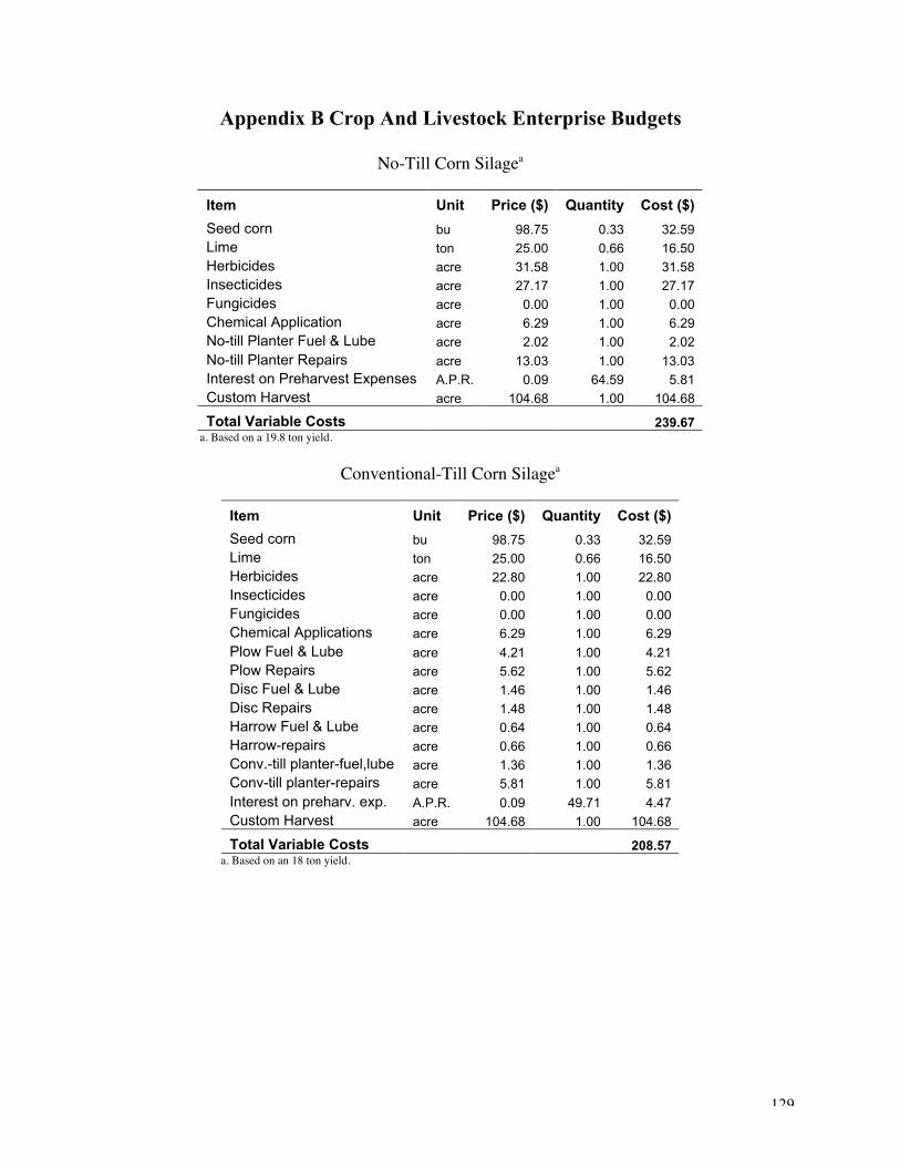
129
Appendix B Crop And Livestock Enterprise Budgets
No-Till Corn Silagea
Item Unit Price ($) Quantity Cost ($)
Seed corn bu 98.75 0.33 32.59Lime ton 25.00 0.66 16.50Herbicides acre 31.58 1.00 31.58Insecticides acre 27.17 1.00 27.17Fungicides acre 0.00 1.00 0.00Chemical Application acre 6.29 1.00 6.29No-till Planter Fuel & Lube acre 2.02 1.00 2.02
No-till Planter Repairs acre 13.03 1.00 13.03Interest on Preharvest Expenses A.P.R. 0.09 64.59 5.81Custom Harvest acre 104.68 1.00 104.68
Total Variable Costs 239.67 a. Based on a 19.8 ton yield.
Conventional-Till Corn Silagea
Item Unit Price ($) Quantity Cost ($)
Seed corn bu 98.75 0.33 32.59Lime ton 25.00 0.66 16.50Herbicides acre 22.80 1.00 22.80Insecticides acre 0.00 1.00 0.00Fungicides acre 0.00 1.00 0.00Chemical Applications acre 6.29 1.00 6.29
Plow Fuel & Lube acre 4.21 1.00 4.21Plow Repairs acre 5.62 1.00 5.62Disc Fuel & Lube acre 1.46 1.00 1.46Disc Repairs acre 1.48 1.00 1.48Harrow Fuel & Lube acre 0.64 1.00 0.64Harrow-repairs acre 0.66 1.00 0.66Conv.-till planter-fuel,lube acre 1.36 1.00 1.36Conv-till planter-repairs acre 5.81 1.00 5.81
Interest on preharv. exp. A.P.R. 0.09 49.71 4.47Custom Harvest acre 104.68 1.00 104.68
Total Variable Costs 208.57 a. Based on an 18 ton yield.

130
No-Till Corn Graina
Item Unit Price ($) Quantity Cost ($)
Seed corn bu 98.75 0.33 32.59Lime ton 25.00 0.66 16.50Herbicides acre 31.58 1.00 31.58Insecticides acre 27.17 1.00 27.17Fungicides acre 0.00 1.00 0.00Chemical Applications acre 6.29 1.00 6.29No-till Planter Fuel & Lube acre 2.02 1.00 2.02No-till Planter Repairs acre 13.03 1.00 13.03Interest on Preharvest Expenses A.P.R. 0.09 64.59 5.81
Custom Harvest acre 53.25 1.00 53.25Hauling costs bu 0.15 132.00 19.80
Total Variable Costs 208.04 a. Based on a 132 bushel yield.
Conventional-Till Corn Graina
Item Unit Price ($) Quantity Cost ($)
Seed corn bu 98.75 0.33 32.59Lime ton 25.00 0.66 16.50Herbicides acre 22.80 1.00 22.80Insecticides acre 0.00 1.00 0.00Fungicides acre 0.00 1.00 0.00Chemical Applications acre 6.29 1.00 6.29
Rotary Cutter Fuel & Lube acre 1.67 1.00 1.67Rotary Cutter Repairs acre 5.09 1.00 5.09Plow Fuel Lube acre 4.21 1.00 4.21Plow Repairs acre 5.62 1.00 5.6218 ft Disc Fuel & Lube acre 1.46 1.00 1.4618 ft Disc Repairs acre 1.48 1.00 1.4812 ft Harrow Fuel & Lube acre 0.64 1.00 0.6412 ft Harrow Repairs acre 0.66 1.00 0.66
Conventional-till Planter Fuel & Lube acre 1.36 1.00 1.36Conventional-till Planter Repairs acre 5.81 1.00 5.81Interest on Preharvest Expenses A.P.R. 0.09 53.09 4.78Custom Harvest acre 53.25 1.00 53.25Hauling bu 0.15 120.00 18.00
Total Variable Costs 182.20 a. Based on a 120 bushel yield.

131
Alfalfa Hay No-Till Establishment
Item Unit Price ($) Quantity Cost ($)Establishment Costs
Seed lbs 3.09 16.00 49.44Boron lbs 3.60 3.00 10.80Lime ton 25.00 2.50 62.50Herbicide-Gramoxone pt 4.25 3.00 12.75Herbicide-sticker pt 2.32 2.00 4.64Herbicide-2-4-D pt 1.81 3.00 5.43
Herbicide-Banvel pt 11.48 1.50 17.22Chemical Applications ac 6.29 1.00 6.2970 hp Rented Seeder Fuel & Lube ac 2.68 1.00 2.6870 hp Rented Seeder Repairs ac 10.05 1.00 10.05Interest on Preharvest Expenses ac 0.09 181.80 16.361st Year Hay Costs
Insecticide-Dimethoate 4EC pt 5.19 0.50 2.60Insecticide-Furadan 4F pt 8.23 0.50 4.12Chemical Applications ac 6.29 1.00 6.29
Interest on Preharvest Expenses ac 0.09 22.87 2.06Custom harvest ac 179.23 1.00 179.23Baler twine bale 0.05 200.00 10.00
Total Variable Costs 402.45

132
Alfalfa Hay Conventional-Till Establishment
Item Unit Price ($) Quantity Cost ($)Establishment Costs
Seed lbs 3.09 20.00 61.80Boron lbs 3.60 3.00 10.80Lime ton 25.00 2.50 62.50Herbicide-Eptam 7E pt 4.43 3.50 15.51Chemical Applications ac 6.29 1.00 6.2970 hp 8 ft Drill Fuel & Lube ac 1.69 1.00 1.69
70 hp 8 ft Drill Repairs ac 3.83 1.00 3.8360 hp 3-16 Plow Fuel & Lube ac 3.37 1.00 3.3760 hp 3-16 Plow Repairs ac 4.61 1.00 4.6170 hp 10 ft Disk Fuel & Lube ac 1.14 2.00 2.2870 hp 10 ft Disk Repairs ac 1.53 2.00 3.0650 hp 12 ft Harrow Fuel & Lube ac 0.64 1.00 0.6450 hp 12 ft Harrow Repairs ac 0.66 1.00 0.6650 hp 12 ft Cultipacker Fuel & Lube ac 0.61 1.00 0.61
50 hp 12 ft Cultipacker Repairs ac 0.74 1.00 0.74Interest on Preharvest Expenses ac 0.09 175.74 15.821st Year Hay Costs
Insecticide-Dimethoate 4EC pt 5.19 0.50 2.60Insecticide-Furadan 4F pt 8.23 0.50 4.12Chemical Applications ac 6.29 1.00 6.29Interest on Preharvest Expenses ac 0.09 22.87 2.06Custom harvest ac 179.23 1.00 179.23Baler twine bale 0.05 200.00 10.00
Total Variable Costs 398.49
Alfalfa Haya
Item Unit Price ($) Quantity Cost ($)
Boron lbs 3.60 3.00 10.80Lime ton 25.00 0.50 12.50Herbicide-Sencor lbs 22.69 0.25 5.67Herbicide-Gramoxone pt 4.25 0.75 3.19Herbicide-Sticker pt 2.32 0.25 0.58Insecticide-Dimethoate 4EC pt 5.19 0.50 2.60Insecticide-Furadan 4F pt 8.23 0.50 4.12Chemical Applications ac 6.29 1.00 6.29Interest on Preharvest Expenses ac 0.09 22.87 2.06
Custom harvest ac 179.23 1.00 179.23Baler twine bale 0.05 200.00 10.00
Total Variable Costs 237.03 a. Based on a five ton yield.

133
Orchard Grass-Clover No-Till Establishmenta
Item Unit Price ($) Quantity Cost ($)Establishment Costs
Seed lbs 2.18 8.00 17.44Red clover seed/inoculant lbs 1.32 6.00 7.92Lime ton 25.00 2.00 50.00Herbicide-Gramoxone pt 4.25 3.00 12.75Herbicide-Sticker pt 2.32 2.00 4.64Herbicide-2-4D pt 1.81 2.00 3.62
Herbicide-Banvel pt 11.48 1.00 11.48Chemical application ac 6.29 1.00 6.2970 hp Rented Seeder Fuel & Lube ac 2.68 1.00 2.6870 hp Rented Seeder Repairs ac 10.05 1.00 10.05Interest on Preharvest Expenses ac 0.09 126.87 11.421st Year Hay Costs
Custom harvest ac 80.08 1.00 80.08Baler Twine-Round bale 0.67 7.50 5.03Interest on Preharvest Expenses ac 0.09 8.23 0.74
Total Variable Costs 224.13 a. For permanent pasture.
Orchard Grass-Clover Conventional-Till Establishmenta
Item Unit Price ($) Quantity Cost ($)Establishment Costs
Seed lbs 2.18 8.00 17.44Red Clover Seed/Inoculant lbs 1.32 6.00 7.92Spring Oats Seed bu 8.04 0.60 4.82Lime ton 25.00 2.00 50.0070 hp 8 ft Drill Fuel & Lube ac 1.69 1.00 1.6970 hp 8 ft Drill Repairs ac 3.83 1.00 3.83
60 hp 3-16 Plow Fuel & Lube ac 3.37 1.00 3.3760 hp 3-16 Plow Repairs ac 4.61 1.00 4.6170 hp 10 ft Disk Fuel & Lube ac 1.14 2.00 2.2870 hp 10 ft Disk Repairs ac 1.53 2.00 3.0650 hp 12 ft Harrow Fuel & Lube ac 0.64 1.00 0.6450 hp 12 ft Harrow Repairs ac 0.66 1.00 0.66Interest on Preharvest Expenses ac 0.09 99.02 8.911st Year Hay Costs
Custom harvest ac 80.08 1.00 80.08Baler Twine-Round bale 0.67 7.50 5.03Interest on Preharvest Expenses ac 0.09 8.23 0.74
Total Variable Costs 195.08 a. For permanent pasture.

134
Permanent Pasture
Item Unit Price ($) Quantity Cost ($)
Red Clover Seed/Inoculant lbs 1.32 2.00 1.32Lime ton 25.00 0.50 3.1350 hp 7-ft. Bushhog Fuel & Lube ac 1.18 1.00 1.1850 hp 7-ft. Bushhog Repairs ac 2.87 1.00 2.8740 hp Cyclone Seeder Fuel & Lube ac 0.61 1.00 0.6140 hp Cyclone Seeder Repairs ac 0.42 1.00 0.42Interest on Preharvest Expenses ac 0.09 4.76 0.43
Total Variable Costs 9.95
Buffer Establishment
Item Unit Price ($) Quantity Cost ($)
Seed (Bluestem) lbs 25.40 2.00 50.80Seed (Switchgrass) lbs 4.75 2.00 9.50Seed (Partridge Peas) lbs 15.00 1.00 15.00
Herbicide-Gramoxone pt 4.25 3.00 12.75Herbicide-Sticker pt 2.32 2.00 4.64Herbicide 2-4-D pt 1.81 2.00 3.62Herbicide-Banvel pt 11.48 1.00 11.48Lime ton 25.00 0.50 12.50Nitrogen lb 0.27 0.00 0.00Phosphate lb 0.24 40.00 9.60Potash lb 0.15 40.00 6.00
Fertilizer Applications ac 6.14 1.00 6.14Rented Seeder Labor hours 7.50 0.55 4.13Rented Seeder Fuel & Lube ac 2.68 1.00 2.68Rented Seeder Repair ac 10.05 1.00 10.05Interest on Preharvest Expenses ac 0.09 158.89 14.30
Total Variable Costs 173.18
Buffer Maintenance
Item Unit Price ($) Quantity Cost ($)
Lime ton 25.00 0.25 6.25
Lime application ac 6.14 0.50 3.07
Bushhog Labor hours 7.50 0.41 3.08
50 hp 7-ft. Bushhog Fuel & Lube ac 1.18 1.00 1.18
50 hp 7-ft. Bushhog Repairs ac 2.87 1.00 2.87
Interest on Preharvest Expenses ac 0.09 8.22 0.74
Total Variable Costs 17.19

135
Appendix C P Delivery Model Code
C.1 ArcView GIS Code
ArcView was used to calculate P deliveries for the population case.'************************************************************************'ArcView3.2 script: rksl-615.ave'Purpose: calculate RKSL portion of USLE for a watershed and slope and' length-across-cell grids used in nps-615.ave script.'Programmer: Tamie Veith - June 15, 2002'Description:' Converts K factor into SI units.' Calculates slope, in degrees and decimal [m/m].' Calculates length-across-cell grid [m].' Calculates USLE S and L factors, both dimensionless.' Creates RKSL grid as R*K*S*L * conversion from Mg to English tons;' final RKSL-US grid in [tons/acre].' Outputs statistics at field-level of cell-level RKSL values, in' [tons/acre] into working directory (filename: "StatsRKSL.dbf").'' Adds a column "Runoff" to the land use file for the NPS script.''Script Dependance:' This script calls the "MakeGTheme" script to display grid themes.' The script lines making this call look like the following:' 'create theme and add to view' theView.AddTheme(av.run("MakeGtheme",{flwaccGrid,"Flow Accumulation"}))' Such lines making this call can be commented out at will to' customize the selection of output themes displayed in the view.'************************************************************************
theView = av.GetActiveDoc'**input data 'Cell width [m] constCellW = 30 'DEM theDEMGrid = theView.FindTheme("Fill1").GetGrid 'watershed grid wshedGrid = theView.FindTheme("Jb-wshed").GetGrid 'K grid in English units KgridENG = theView.FindTheme("Kfactus").GetGrid 'R factor in SI units constRfactor = 2800 'characteristic slope length for L factor in SI units [m] constSlopeLength = 45 'Landuse (fields) shape file theMPIDftab = theView.FindTheme("NRCS-landuse.shp").GetFTab theFieldIDfield = theMPIDftab.FindField("Field_id")
'**calc slope grids 'decimal slope grid slopeDecimalGrid = (theDEMGrid.Slope (1, TRUE))/100 'save data set slopeDecimalGrid.SaveDataSet("slopedec".asFileName) 'create theme and add to view

136
theView.AddTheme(av.run("MakeGtheme",{slopeDecimalGrid,"Slope inm/m"}))
'degree slope grid slopeDegreeGrid = theDEMGrid.Slope (1, FALSE) 'convert to radians slopeRadGrid = slopeDegreeGrid*(Number.getPi.asGrid)/(180.asGrid)
'**create flow direction and flow accumulation grids 'calc flow direction flowDirGrid = theDEMGrid.FlowDirection (FALSE) 'save data set flowDirGrid.SaveDataSet("FlowDir".asFileName) 'create theme and add to view theView.AddTheme(av.run("MakeGtheme",{flowDirGrid,"Flow Direction"})) 'make flow accumulation for later flwaccGrid = flowDirGrid.FlowAccumulation(NIL) 'save data set flwaccGrid.SaveDataSet("FlowAcc".asFileName) 'create theme and add to view theView.AddTheme(av.run("MakeGtheme",{flwaccGrid,"Flow Accumulation"}))
'**create flow-length-across-cell grid 'locate cells with diagonal flow directions tempGrid1=(flowDirGrid = 2.AsGrid) or (flowDirGrid = 8.AsGrid) or (flowDirGrid = 32.AsGrid) or (flowDirGrid = 128.AsGrid) 'assign diagonal flow cells a length of cell width times SQRT(2) tempGrid2=(tempGrid1 * constCellW.AsGrid * 2.Sqrt.AsGrid) 'locate cells with non-diagonal flow directions tempGrid1=(flowDirGrid= 1.AsGrid) or (flowDirGrid = 4.AsGrid) or (flowDirGrid = 16.AsGrid) or (flowDirGrid = 64.AsGrid) 'assign non-diagonal flow cells a length of cell width and combine bothtemp grids into one grid lengthGrid=tempGrid2+(tempGrid1 * constCellW.AsGrid)
'save data set lengthGrid.SaveDataSet("lngtcell".asFileName) 'create theme and add to view theView.AddTheme(av.run("MakeGtheme",{lengthGrid,"Length Across Cell"}))
'**convert K factor to SI units (conversion = 0.1317) KgridSI = KgridENG*(0.1317)' 'save data set' KgridSI.SaveDataSet("Kfact-si".asFileName)' 'create theme and add to view' theView.AddTheme(av.run("MakeGtheme",{KgridSI,"Kfact-si"}))
'**calc L factor for USLE 'create beta grid betaNumGrid = (slopeRadGrid.Sin)/((0.0896).AsGrid) betaDenomGrid =((3.AsGrid)*((slopeRadGrid.Sin).Pow(0.8)))+((0.56).AsGrid) betaGrid = betaNumGrid/betaDenomGrid 'create m grid mGrid = betaGrid/(1.AsGrid+betaGrid) 'calculate L factor lGrid = ((constSlopeLength.AsGrid)/(22.AsGrid)).Pow(mGrid)

137
'save data set lGrid.SaveDataSet("Lfact".asFileName) 'create theme and add to view theView.AddTheme(av.run("MakeGtheme",{lGrid,"Lfact"}))
'**calc S factor for USLE 'locate cells with slope < 9% flagShortGrid=(slopeDegreeGrid < ((5.1428).AsGrid)) 'assign S-factor for short slopes tempGrid1=( (((10.8).AsGrid)*(slopeRadGrid.Sin)) + ((0.03).AsGrid))*flagShortGrid 'locate cells with slope >= 9% flagLongGrid=(slopeDegreeGrid >= ((5.1428).AsGrid)) 'assign S-factor for long slopes SGrid=tempGrid1+(( (((16.8).AsGrid)*(slopeRadGrid.Sin)) -((0.50).AsGrid))*flagLongGrid) 'save data set SGrid.SaveDataSet("Sfact".asFileName) 'create theme and add to view theView.AddTheme(av.run("MakeGtheme",{SGrid,"Sfact"}))
'**calc RKSL grid in Eng units (conversion: (ton/ac) = (Mg/ha) / 2.242) 'create grid theRKSLgrid = wshedGrid*(constRfactor.AsGrid)*KgridSI*SGrid*LGrid/(2.242) 'save data set theRKSLgrid.SaveDataSet("RKSL-us".asFileName) 'create theme and add to view theView.AddTheme(av.run("MakeGtheme",{theRKSLgrid,"RKSL-us"}))
'**Calculate statistics of RKSL by field in [tons/acre] (show mean overfield)** theRKSLgrid.ZonalStatsTable (theMPIDftab, Prj.MakeNull, theFieldIDfield, TRUE, "StatsRKSL.dbf".AsFileName) FieldRKSLGrid = theRKSLgrid.ZonalStats (#GRID_STATYPE_MEAN, theMPIDftab, Prj.MakeNull,theFieldIDfield, TRUE) '** create theme and add to view theView.AddTheme(av.run("MakeGtheme",{FieldRKSLGrid,"Avg Field-levelRKSL [tons/acre]"}))
'*** add runoff column to landuse table '**edit fields/landuse shape file theMPIDftab.SetEditable(TRUE) 'make new column for runoff by field [in] and add to table theRunoffField = Field.Make("Runoff",#FIELD_DOUBLE,16,2) theMPIDftab.AddFields({theRunoffField})
theMPIDftab.SetEditable(FALSE)
'************************************************************************'ArcView3.2 script: nps-615.ave'Purpose: predicting sediment-bound P from a watershed.'Programmer: Tamie Veith - June 15, 2002'Description:' DATA PREPARATION SECTION' Reads in management practice ID and phosphorous concentrations
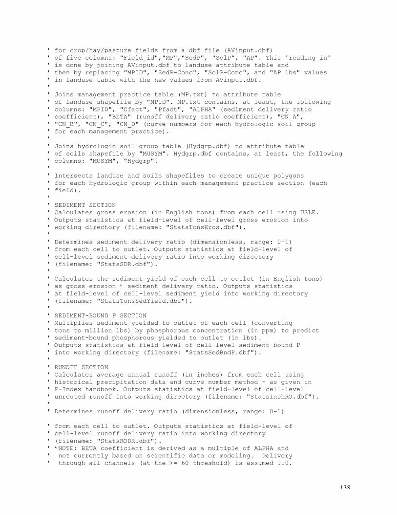
138
' for crop/hay/pasture fields from a dbf file (AVinput.dbf)' of five columns: "Field_id","MP","SedP", "SolP", "AP". This 'reading in'' is done by joining AVinput.dbf to landuse attribute table and' then by replacing "MPID", "SedP-Conc", "SolP-Conc", and "AP_lbs" values' in landuse table with the new values from AVinput.dbf.'' Joins management practice table (MP.txt) to attribute table' of landuse shapefile by "MPID". MP.txt contains, at least, the following' columns: "MPID", "Cfact", "Pfact", "ALPHA" (sediment delivery ratio' coefficient), "BETA" (runoff delivery ratio coefficient), "CN_A",' "CN_B", "CN_C", "CN_D" (curve numbers for each hydrologic soil group' for each management practice).'' Joins hydrologic soil group table (Hydgrp.dbf) to attribute table' of soils shapefile by "MUSYM". Hydgrp.dbf contains, at least, the following' columns: "MUSYM", "Hydgrp".'' Intersects landuse and soils shapefiles to create unique polygons' for each hydrologic group within each management practice section (each' field).'' SEDIMENT SECTION' Calculates gross erosion (in English tons) from each cell using USLE.' Outputs statistics at field-level of cell-level gross erosion into' working directory (filename: "StatsTonsEros.dbf").'' Determines sediment delivery ratio (dimensionless, range: 0-1)' from each cell to outlet. Outputs statistics at field-level of' cell-level sediment delivery ratio into working directory' (filename: "StatsSDR.dbf").'' Calculates the sediment yield of each cell to outlet (in English tons)' as gross erosion * sediment delivery ratio. Outputs statistics' at field-level of cell-level sediment yield into working directory' (filename: "StatsTonsSedYield.dbf").'' SEDIMENT-BOUND P SECTION' Multiplies sediment yielded to outlet of each cell (converting' tons to million lbs) by phosphorous concentration (in ppm) to predict' sediment-bound phosphorous yielded to outlet (in lbs).' Outputs statistics at field-level of cell-level sediment-bound P' into working directory (filename: "StatsSedBndP.dbf").'' RUNOFF SECTION' Calculates average annual runoff (in inches) from each cell using' historical precipitation data and curve number method - as given in' P-Index handbook. Outputs statistics at field-level of cell-level' unrouted runoff into working directory (filename: "StatsInchRO.dbf").'' Determines runoff delivery ratio (dimensionless, range: 0-1)
' from each cell to outlet. Outputs statistics at field-level of' cell-level runoff delivery ratio into working directory' (filename: "StatsRODR.dbf").' *NOTE: BETA coefficient is derived as a multiple of ALPHA and' not currently based on scientific data or modeling. Delivery' through all channels (at the >= 60 threshold) is assumed 1.0.

139
'' Calculates the runoff yield of each cell to outlet (in inches)' as unrouted runoff * runoff delivery ratio. Outputs statistics' at field-level of cell-level runoff yield into working directory' (filename: "StatsInchROYield.dbf").'' APPLIED P SECTION' Grids values of applied P in lbs. Applied P was entered' through the AVinput.dbf file in lbs for the decision fields.' These imputs are copied over to the column that already contains' the applied values for fixed fields (these inputs entered one time' in the landuse file in the same way as the sed- and sol-P values.)
' SOLUBLE P SECTION' Multiplies routed runoff yielded to outlet of each cell (converting' inches to million lbs) by phosphorous concentration ('in ppm) and adds' 4% of the applied P (in lbs) to predict soluble phosphorous yielded' to outlet (in lbs).' Outputs statistics at field-level of cell-level' soluble P into working directory (filename: "StatsSolP.dbf").''' TOTAL P SECTION' Adds cell-level sediment-bound and soluble P to get total surface' P yielded to outlet in lbs. Outputs statistics' at field-level of cell-level P yield into working directory' (filename: "StatsTotP.dbf").
' *NOTE: SUBSURFACE COMPONENTS are not considered.'''Script Dependence:' This script calls the "intersec" script to automate intersection' of the land use and soils shapefiles.'' This script calls the "MakeGTheme" script to display grid themes.''Output Customization:' The script lines calling the "MakeGTheme" script look like:' 'create theme and add to view' theView.AddTheme(av.run("MakeGtheme",{flwaccGrid,"Flow Accumulation"}))' Such lines can be commented out at will to customize the selection of' output themes displayed in the view (and make the script run faster.)''' The script lines calculating statistics and outputing the results as atable' and a theme look like:' '* Calculate statistics of sediment yield to outlet by field in [tons](show sum over field)**' theCellTotSedLossGrid.ZonalStatsTable (theMPIDftab, Prj.MakeNull,' theFieldIDfield, TRUE,"StatsTonsSedYield.dbf".AsFileName)' theTotalFieldSedLossGrid = theCellTotSedLossGrid.ZonalStats' (#GRID_STATYPE_SUM, theMPIDftab, Prj.MakeNull,theFieldIDfield, TRUE)' '** create theme and add to view

140
' theView.AddTheme(av.run("MakeGtheme",{theTotalFieldSedLossGrid,"Totalsed yield by field [tons]"}))' Such lines can be commented out at will to customize the selection of' output tables and themes provided (and make the script run faster.)''************************************************************************
'***Data Preparation Section ******************************************** '***Set Constant Values********************************************* cnstCellArea = 0.09 'cell size [ha] cnstCellAreaUS = cnstCellArea/(0.4047) 'cell size [ac]
'**set cell size and extent for shapefile-to-grid conversion theCellSize = 30 'length of one side of square cell [m] theExtent = Rect.MakeXY(669830.142059,4253895,683150.142059,4271685) 'MakeXY(x1,y1,x2,y2) that is, (left, bottom, right, top)
'**identify Virginia climatic zone for determining average annual runoff theClimZn = 5 'Central Mountain, including Rockingham county
'***Locate Input Data*********************************************** theView = av.GetActiveDoc
'**change name of field shape file, if needed** theMPIDtheme = theView.FindTheme("Nrcs-landuse.shp") theMPIDftab = theMPIDtheme.GetFTab theFieldIDfield = theMPIDftab.FindField("Field_id") theMPIDfield = theMPIDftab.FindField("Mpid") theSedPConcfield = theMPIDftab.FindField("SedP_Conc") theSolPConcfield = theMPIDftab.FindField("SolP_Conc") theAPfield = theMPIDftab.FindField("AP_lbs")
theFlowDirGrid = theView.FindTheme("Flow Direction").GetGrid theFlowAccumGrid = theView.FindTheme("Flow Accumulation").GetGrid theRKSLgrid = theView.FindTheme("RKSL-us").GetGrid theLengthGrid = theView.FindTheme("Length Across Cell").GetGrid theSlopeDecGrid = theView.FindTheme("Slope in m/m").GetGrid
'**change name of soils shape file, if needed** theSoilstheme = theView.FindTheme("Soil_srg.shp") theSoilsftab = theSoilstheme.GetFTab
theCNvtab = av.GetProject.FindDoc("CN.txt").GetVTab 'locate proper columns in CN table theClimZnfield = theCNvtab.FindField("Div"+theClimZn.AsString) theCNfield = theCNvtab.FindField("CN")
'***Read in MPIDs and P-conc from input table************************ 'That is, replace MPID, SedP_conc, and SolP_conc values in landuse 'attribute table with values provided by input file. For all fields without 'values in the input file, the existing MPID, SedP_conc, and SolP_conc 'values remain unchanged. This replacement is intended for reflecting 'changes on production land as a result of management practice changes 'to that land.

141
'***join input data into landuse attribute table**** theMPIDftab.UnjoinAll theInputvtab = av.GetProject.FindDoc("AVinput.dbf").GetVTab theJoinFromfield = theInputvtab.FindField("Field_id") theJoinTofield = theFieldIDfield theMPIDftab.Join (theJoinTofield,theInputvtab,theJoinFromfield)
'***replace old values with new data**** theMPinputField = theMPIDftab.FindField("Mp") theSedPinputField = theMPIDftab.FindField("SedP") theSolPinputField = theMPIDftab.FindField("SolP") theApplPinputField = theMPIDftab.FindField("AP")
theMPIDftab.SetEditable(TRUE) for each record in theMPIDftab 'replace existing MPID with new value for records with an input value theMPinputValue = theMPIDftab.ReturnValue(theMPinputField,record) if ((theMPinputValue.IsNull).Not) then theMPIDftab.SetValue(theMPIDField,record,theMPinputValue) end 'replace existing SedP_Conc with new value for records with an inputvalue theSedPinputValue = theMPIDftab.ReturnValue(theSedPinputField,record) if ((theSedPinputValue.IsNull).Not) then theMPIDftab.SetValue(theSedPConcfield,record,theSedPinputValue) end 'replace existing SolP_Conc with new value for records with an inputvalue theSolPinputValue = theMPIDftab.ReturnValue(theSolPinputField,record) if ((theSolPinputValue.IsNull).Not) then theMPIDftab.SetValue(theSolPConcfield,record,theSolPinputValue) end 'replace existing AP_lbs with new value for records with an input value theApplPinputValue = theMPIDftab.ReturnValue(theApplPinputField,record) if ((theApplPinputValue.IsNull).Not) then theMPIDftab.SetValue(theAPfield,record,theApplPinputValue) end end 'for each theMPIDftab.SetEditable(FALSE)
'***join MP.txt table to landuse attribute table (theMPIDftab)*********** theMP_TABLEvtab = av.GetProject.FindDoc("MP.txt").GetVTab theJoinFromfield = theMP_TABLEvtab.FindField("Mpid") theJoinTofield = theMPIDField theMPIDftab.Join (theJoinTofield,theMP_TABLEvtab,theJoinFromfield)
'***join Hydgrp.dbf table to soil attribute table (theSoilsftab)********** theHydgrp_TABLEvtab = av.GetProject.FindDoc("hydgrp.dbf").GetVTab theJoinFromfield = theHydgrp_TABLEvtab.FindField("Musym") theJoinTofield = theSoilsftab.FindField("Musym") theSoilsftab.Join (theJoinTofield,theHydgrp_TABLEvtab,theJoinFromfield)
'***intersect landuse and soils********** '**caution - intersect may fail if joins are performed multiple times. theSoilbyFLDfname =av.run("intersec",{theView,theMPIDtheme,theSoilstheme,"SoilbyFld.shp".AsFileName})

142
theSoilbyFLDtheme = theView.FindTheme("SoilbyFld.shp") theSbyFftab = theSoilbyFLDtheme.GetFtab 'locate hydrological soil group and runoff column in SoilbyFld table theHydGrpfield = theSbyFftab.FindField("Hydgrp") theRunoffField = theSbyFftab.FindField("Runoff")
'***END Data Preparation Section ******************************************
'***Sediment Section*********************************************** '***Calculate Gross Erosion ************************************* '**grid C factor of USLE equation theCfield = theMPIDftab.FindField("Cfact") theCgrid = Grid.MakeFromFTab(theMPIDftab, Prj.MakeNull, theCfield,{theCellSize,theExtent}) '** create theme and add to view theView.AddTheme(av.run("MakeGtheme",{theCgrid,"C factor"}))
'**grid P factor of USLE equation thePfield = theMPIDftab.FindField("Pfact") thePgrid = Grid.MakeFromFTab(theMPIDftab, Prj.MakeNull, thePfield,{theCellSize,theExtent}) '** create theme and add to view' theView.AddTheme(av.run("MakeGtheme",{thePgrid,"input P factor"})) 'calc P for contour truePgrid= (((thePgrid = 2.AsGrid) and (theSlopeDecGrid<=(0.02).AsGrid))*0.6) +(((thePgrid = 2.AsGrid) and (theSlopeDecGrid >(0.02).AsGrid)and(theSlopeDecGrid <=(0.07).AsGrid))*0.5) +(((thePgrid = 2.AsGrid) and (theSlopeDecGrid >(0.07).AsGrid)and(theSlopeDecGrid <=(0.12).AsGrid))*0.6) +(((thePgrid = 2.AsGrid) and (theSlopeDecGrid >(0.12).AsGrid)and(theSlopeDecGrid <=(0.18).AsGrid))*0.8) +(((thePgrid = 2.AsGrid) and (theSlopeDecGrid >(0.18).AsGrid)and(theSlopeDecGrid <=(0.24).AsGrid))*0.9) +(((thePgrid = 2.AsGrid) and (theSlopeDecGrid >(0.24).AsGrid))*1) +((thePgrid = 1.AsGrid) *1) '** create theme and add to view' theView.AddTheme(av.run("MakeGtheme",{truePgrid,"calc P factor"}))
'**calculate USLE cell-level gross erosion 'by cell in [tons] theErosGrid = theRKSLgrid*theCgrid*truePgrid*cnstCellAreaUS.asGrid '** create theme and add to view theView.AddTheme(av.run("MakeGtheme",{theErosGrid,"Gross Erosion bycell in tons"}))
'* Calculate statistics of gross erosion to outlet by field in [tons](show sum over field)** theErosGrid.ZonalStatsTable (theMPIDftab, Prj.MakeNull, theFieldIDfield, TRUE,"StatsTonsEros.dbf".AsFileName) FieldErosGrid = theErosGrid.ZonalStats (#GRID_STATYPE_SUM, theMPIDftab, Prj.MakeNull,theFieldIDfield, TRUE) '** create theme and add to view

143
theView.AddTheme(av.run("MakeGtheme",{FieldErosGrid,"Total Field-levelErosion [tons]"}))
'***Route Sediment Delivery*************************************** '**locate within landuse shapefile and grid ALPHA factor of sedimentdelivery equation theALPHAfield = theMPIDftab.FindField("Alpha") theALPHAgrid = Grid.MakeFromFTab(theMPIDftab, Prj.MakeNull,theALPHAfield, {theCellSize,theExtent}) '** create theme and add to view ' theView.AddTheme(av.run("MakeGtheme",{theALPHAgrid,"Alpha grid"}))
'**calculate delivery from overland cell with equation:alpha*SQRT(slope/length) theDgrid = theALPHAgrid*((theSlopeDecGrid/theLengthGrid).SQRT) '** create theme and add to view' theView.AddTheme(av.run("MakeGtheme",{theDgrid,"Unbounded DeliveryFunction by Cell"}))
'**calculate delivery to include channel cells; set max and min deliveryrates as follows: 'limit (delivery > 1) to 1 'change 0 delivery to 0.001 to prevent taking natural log (0) theMaxDgrid = ( ( theDgrid=0 ) * (0.001)) +( ( ((theDgrid>0) and (theDgrid<1)) and(theFlowAccumGrid<60) ) * (theDgrid) ) +( ( (theDgrid>=1) and (theFlowAccumGrid<60) ) * (1)) +( ( (theFlowAccumGrid>=60) and (theFlowAccumGrid<200)) * (0.98) ) +( ( (theFlowAccumGrid>=200)) * (0.9998) ) '** create theme and add to view' theView.AddTheme(av.run("MakeGtheme",{theMaxDgrid,"Delivery Function byCell"}))
'**route sediment delivery to outlet theLnDgrid = (theMaxDgrid.Log) *(-1) 'mult by -1 to make ln numbers pos for flow accum '** create theme and add to view' theView.AddTheme(av.run("MakeGtheme",{theLnDgrid,"-ln(Del)"}))
theDelAccumGrid =theFlowDirGrid.FlowLength((theLnDgrid/theLengthGrid),FALSE) 'accumulate downstream '** create theme and add to view' theView.AddTheme(av.run("MakeGtheme",{theDelAccumGrid,"flowlength (-ln(Del)/length)"}))
theExpDwnstrmAccum = (theDelAccumGrid*(-1)).Exp 'mult by -1 to return ln numbers to proper sign '** create theme and add to view theView.AddTheme(av.run("MakeGtheme",{theExpDwnstrmAccum,"sed del fromcell to outlet"}))

144
'* Calculate statistics of Sediment Delivery Ratio to Outlet by Field(show avg by field)** theExpDwnstrmAccum.ZonalStatsTable (theMPIDftab, Prj.MakeNull, theFieldIDfield, TRUE,"StatsSDR.dbf".AsFileName) avgSedDelGrid = theExpDwnstrmAccum.ZonalStats (#GRID_STATYPE_MEAN, theMPIDftab, Prj.MakeNull,theFieldIDfield, TRUE) '** create theme and add to view theView.AddTheme(av.run("MakeGtheme",{avgSedDelGrid,"average field-level sed del"}))
'***Report Total Sediment Yield ************************************* '**Get total sediment yielded to outlet by each field theCellTotSedLossGrid = theErosGrid*theExpDwnstrmAccum '* Calculate statistics of sediment yield to outlet by field in [tons](show sum over field)** theCellTotSedLossGrid.ZonalStatsTable (theMPIDftab, Prj.MakeNull, theFieldIDfield, TRUE,"StatsTonsSedYield.dbf".AsFileName) theTotalFieldSedLossGrid = theCellTotSedLossGrid.ZonalStats (#GRID_STATYPE_SUM, theMPIDftab, Prj.MakeNull,theFieldIDfield, TRUE) '** create theme and add to view theView.AddTheme(av.run("MakeGtheme",{theTotalFieldSedLossGrid,"Totalsed yield by field [tons]"}))
'***END Sediment Section***************************************************
'***Sediment-bound Phosphorous Section************************************* '**locate within landuse shapefile and grid Sed-bnd P concentration theSedBndPconcField = theMPIDftab.FindField("SedP_Conc") theSedBndPconcGrid = Grid.MakeFromFTab(theMPIDftab, Prj.MakeNull, theSedBndPconcField, {theCellSize,theExtent}) '** create theme and add to view theView.AddTheme(av.run("MakeGtheme",{theSedBndPconcGrid,"Sed-bnd Pgrid"}))
'**Get total sediment-bound P yielded to outlet by each field 'NOTE from P-Index handbook: 'For use in the P index, the RUSLE soil loss in tons/acre 'must be multiplied by 0.002 to convert the value to million lbssediment/acre. 'Here soil loss is in tons so 0.002 conversion results in million lbs 'SedPconc is in ppm, so sed*Pconc => units in lbs theCellSedBndPGrid = theCellTotSedLossGrid*theSedBndPconcGrid*0.002 '* Calculate statistics of sed-bound P to outlet by field (show sum overfield)** theCellSedBndPGrid.ZonalStatsTable (theMPIDftab, Prj.MakeNull, theFieldIDfield, TRUE,"StatsSedBndP.dbf".AsFileName) theTotalSedBndPGrid = theCellSedBndPGrid.ZonalStats (#GRID_STATYPE_SUM, theMPIDftab, Prj.MakeNull,theFieldIDfield, TRUE) '** create theme and add to view theView.AddTheme(av.run("MakeGtheme",{theTotalSedBndPGrid,"Total sed-bound P by field [lbs]"}))

145
'***END Sediment-bound Phosphorous Section*********************************
'***Runoff Section*********************************************** '***Locate avg annual runoff based on curve number *********************** theSbyFftab.SetEditable(TRUE) for each i in theSbyFftab 'get the hydrological soil group for the section theHydGrpvalue = theSbyFftab.ReturnValue(theHydGrpfield,i) 'look through hydrologic group columns to get matching CN CNvalue = theSbyFftab.ReturnValueNumber (theSbyFftab.FindField("Cn_"+theHydGrpvalue.AsString), i) 'look through CN table to get corresponding runoff for each j in theCNvtab if (CNvalue = theCNvtab.ReturnValue(theCNfield, j)) then 'assign the value for this CN and correct climate as the annualrunoff [inches]
theSbyFftab.SetValue(theRunoffField,i,(theCNvtab.ReturnValue(theClimZnfield,j))) 'quite loop break end 'if CNvalue = value of current row in CN table end 'for each j in theCNvtab end 'for each i in theSbyFftab theSbyFftab.SetEditable(FALSE)
'**grid Runoff (inches) theRunoffgrid = Grid.MakeFromFTab(theSbyFftab, Prj.MakeNull, theRunoffField, {theCellSize,theExtent}) '** create theme and add to view theView.AddTheme(av.run("MakeGtheme",{theRunoffgrid,"Unrouted Runoffgrid [inches]"}))
'* Calculate statistics of runoff by field in [inches] (show sum overfield)** theRunoffgrid.ZonalStatsTable (theMPIDftab, Prj.MakeNull, theFieldIDfield, TRUE, "StatsInchRO.dbf".AsFileName) FieldROGrid = theRunoffgrid.ZonalStats (#GRID_STATYPE_SUM, theMPIDftab, Prj.MakeNull,theFieldIDfield, TRUE) '** create theme and add to view theView.AddTheme(av.run("MakeGtheme",{FieldROGrid,"Total Field-levelUnrouted Runoff [inches]"}))
'***Route runoff by a runoff delivery factor ************************ '**locate within landuse shapefile and grid BETA factor of runoffdelivery equation theBETAfield = theSbyFftab.FindField("BETA") theBETAgrid = Grid.MakeFromFTab(theSbyFftab, Prj.MakeNull, theBETAfield,{theCellSize,theExtent}) '** create theme and add to view theView.AddTheme(av.run("MakeGtheme",{theBETAgrid,"Beta grid"}))
'**calculate delivery from overland cell with equation:beta*SQRT(slope/length)

146
theRODgrid = theBETAgrid*((theSlopeDecGrid/theLengthGrid).SQRT) '** create theme and add to view theView.AddTheme(av.run("MakeGtheme",{theRODgrid,"Unbounded RO DeliveryFunction by Cell"}))
'**calculate delivery to include channel cells; set min delivery rate asfollows: 'a minimum value of 0 delivery is set when permeability allows completeinfiltration 'but change 0 delivery to 0.001 to prevent taking natural log (0) 'limit (delivery > 1) to 1 'full delivery is assumed in all channels theMaxRODGrid = ( ( theRODgrid=0 ) * (0.001) ) +(( ((theRODgrid>0) and (theRODgrid<1)) and (theFlowAccumGrid<60)) *(theRODgrid)) +( ( (theRODgrid>=1) and (theFlowAccumGrid<60) ) * (1)) +( ( theFlowAccumGrid>=60 ) *(1) ) '** create theme and add to view theView.AddTheme(av.run("MakeGtheme",{theMaxRODGrid,"RO DeliveryFunction by Cell"}))
'**route delivery to outlet theLnRgrid = (theMaxRODGrid.Log) *(-1) 'mult by -1 to make ln numbers pos for flow accum '** create theme and add to view theView.AddTheme(av.run("MakeGtheme",{theLnRgrid,"-ln(Runoff Del)"}))
theRAccumGrid =theFlowDirGrid.FlowLength((theLnRgrid/theLengthGrid),FALSE) 'accumulate downstream '** create theme and add to view theView.AddTheme(av.run("MakeGtheme",{theRAccumGrid,"flowlength (-ln(Runoff Del)/length)"}))
theRExpDwnstrmAccum = (theRAccumGrid*(-1)).Exp 'mult by -1 to return ln numbers to proper sign '** create theme and add to view theView.AddTheme(av.run("MakeGtheme",{theRExpDwnstrmAccum,"DownstreamRunoff Delivery Surface"}))
'* Calculate Average Runoff Delivery Ratio to Outlet by Field ** theRExpDwnstrmAccum.ZonalStatsTable (theMPIDftab, Prj.MakeNull, theFieldIDfield, TRUE, "StatsRODR.dbf".AsFileName) avgRDelGrid = theRExpDwnstrmAccum.ZonalStats (#GRID_STATYPE_MEAN, theMPIDftab, Prj.MakeNull,theFieldIDfield, TRUE) '** create theme and add to view theView.AddTheme(av.run("MakeGtheme",{avgRDelGrid,"Average runoffdelivery ratio to outlet by field"}))
'***Report Total Runoff ************************************* '**Get total runoff yielded to outlet by each field [inches] theCellTotRunoffGrid = theRunoffgrid*theRExpDwnstrmAccum '* Calculate statistics of runoff yield to outlet by field in [inches](show sum over field)**

147
theCellTotRunoffGrid.ZonalStatsTable (theMPIDftab, Prj.MakeNull, theFieldIDfield, TRUE,"StatsInchROYield.dbf".AsFileName) theTotalFieldROGrid = theCellTotRunoffGrid.ZonalStats (#GRID_STATYPE_SUM, theMPIDftab, Prj.MakeNull,theFieldIDfield, TRUE) '** create theme and add to view theView.AddTheme(av.run("MakeGtheme",{theTotalFieldROGrid,"Totalrunoff yield by field [inches]"}))
'***END Runoff Section***************************************************
'***Applied Phosphorous Section************************************* '**locate within landuse shapefile and grid Applied P concentration theApplPGrid = Grid.MakeFromFTab(theMPIDftab, Prj.MakeNull, theAPfield, {theCellSize,theExtent}) '** create theme and add to view theView.AddTheme(av.run("MakeGtheme",{theApplPGrid,"Applied Pgrid[lbs]"}))
'***END Applied Phosphorous Section*********************************
'***Soluble Phosphorous Section (with 4% of applied P added) **************** '**locate within landuse shapefile and grid Soluble P concentration theSolPconcField = theMPIDftab.FindField("SolP_Conc") theSolPconcGrid = Grid.MakeFromFTab(theMPIDftab, Prj.MakeNull, theSolPconcField, {theCellSize,theExtent}) '** create theme and add to view theView.AddTheme(av.run("MakeGtheme",{theSolPconcGrid,"Sol P grid"}))
'**Get total soluble P yielded to outlet by each field 'NOTE from P-Index handbook 'The values selected from Table 4 [CN.txt] must be multiplied by 0.22651 'to convert from inches to million lbs/acre. 'Then multiply by cell size in ac to get [million lbs] 'The SolPconc is in ppm, so final units are [mill lbs]*[ppm] = lbs theCellSolPGrid =(theCellTotRunoffGrid*(0.22651)*cnstCellAreaUS*theSolPconcGrid) +(theApplPGrid* 0.04*cnstCellAreaUS) '* Calculate statistics of soluble P to outlet by field (show sum overfield)** theCellSolPGrid.ZonalStatsTable (theMPIDftab, Prj.MakeNull, theFieldIDfield, TRUE,"StatsSolP.dbf".AsFileName) theTotalSolPGrid = theCellSolPGrid.ZonalStats (#GRID_STATYPE_SUM, theMPIDftab, Prj.MakeNull,theFieldIDfield, TRUE) '** create theme and add to view theView.AddTheme(av.run("MakeGtheme",{theTotalSolPGrid,"Total solubleP by field [lbs]"}))
'***END Soluble Phosphorous Section*********************************

148
'***Total Phosphorous Section************************************* 'Total P = sediment-bound + soluble theCellTotalPgrid = theCellSedBndPGrid + theCellSolPGrid '* Calculate statistics of total P to outlet by field (show sum overfield)** theCellTotalPgrid.ZonalStatsTable (theMPIDftab, Prj.MakeNull, theFieldIDfield, TRUE,"StatsTotP.dbf".AsFileName) theTotalPGrid = theCellTotalPgrid.ZonalStats (#GRID_STATYPE_SUM, theMPIDftab, Prj.MakeNull,theFieldIDfield, TRUE) '** create theme and add to view theView.AddTheme(av.run("MakeGtheme",{theTotalPGrid,"Total surface P byfield [lbs]"}))
'***END Total Phosphorous Section*********************************
C.2 GAMS Code
GAMS was used to calculate P deliveries for the representative farm, mega farm and typicalfarm cases.$Title Physical Model for P-Control Analysis
*************** SETS ******************************************************
SETS F Farms /1*11/
FLDID Fields /1*72, 101*172/
FF(F,FLDID) Fields matched to farms /$INCLUDE "c:\rungams\data\PM_farmfields.inc" /
MP Management Practice ID /2*21/
HSG hydrologic soil groups /A, B, C, D/
FLDMP(F,FLDID,MP) fields with MPID /$INCLUDE "c:\rungams\data\PM_fldmpid.inc" /
FLDHSG(F,FLDID,HSG) fields with HSG /$INCLUDE "c:\rungams\data\PM_fldhsg.inc" /

149
;
*************** TABLES and other DATA *************************************
*Table Runoff below: Runoff as determined by the VA P-Index uses a curvenumber and the*field's climatic zone. The curve number is determined by a field'shydrologic soil group*and its management practice. Because all the fields in this study are inclimatic zone 5,*the curve numbers in the table were replaced by their corresponding runofffigure;*thereby eliminating one step.
TABLE RUNOFF(MP,HSG) average annual runoff [inches] A B C D
2 0.64 2.39 5.14 7.953 0.64 2.39 5.14 7.954 0.64 2.39 5.14 7.955 0.64 2.39 5.14 7.956 0.48 1.70 5.14 7.957 0.48 1.70 5.14 7.958 0.48 1.70 5.14 7.959 0.48 1.70 5.14 7.9510 0.48 1.70 5.14 7.9511 0.48 1.70 5.14 7.9512 0.48 1.70 5.14 7.9513 0.48 1.70 5.14 7.9514 0.00 0.48 4.61 6.3815 0.00 0.48 4.61 6.3816 0.00 0.48 4.61 6.3817 0.00 0.48 4.61 6.3818 0.00 0.36 4.14 6.3819 0.00 0.36 4.14 6.3820 0.00 0.27 1.52 2.9821 0.00 0.27 1.52 2.98
PARAMETER MPFACTORS(MP,*) management factors;$LIBINCLUDE XLIMPORT MPFACTORS c:\rungams\data\fm_crop&live.xls mpfactors
PARAMETER CFACTOR(MP) crop factor for USLE; LOOP (MP, CFACTOR(MP) = MPFACTORS(MP,'CFACTOR'));
*************** Parameters *********************************************
PARAMETER FLDFACTORS(FLDID,*) field factors and attributes;$LIBINCLUDE XLIMPORT FLDFACTORSc:\rungams\data\FM_farmdata_typical_buffer.xls FLDFACTORS
PARAMETER ACRES(F,FLDID) field size [acres];LOOP (F,LOOP (FLDID,ACRES(F,FLDID)$FF(F,FLDID) = FLDFACTORS(FLDID,'ACRES');));
PARAMETER RHO(F,FLDID) sediment P concentration [ppm];

150
LOOP (F,LOOP (FLDID,RHO(F,FLDID)$FF(F,FLDID) = FLDFACTORS(FLDID,'RHO');));
PARAMETER SIGMA(F,FLDID) runoff P concentration [ppm];LOOP (F,LOOP (FLDID,SIGMA(F,FLDID)$FF(F,FLDID) = FLDFACTORS(FLDID,'SIGMA');));
PARAMETER RKLS(F,FLDID) product of USLE factors [tons per acre];LOOP (F,LOOP (FLDID,RKLS(F,FLDID)$FF(F,FLDID) = FLDFACTORS(FLDID,'RKLS');));
PARAMETER D(F,FLDID) sediment delivery ratio [dimensionless];LOOP (F,LOOP (FLDID,D(F,FLDID)$FF(F,FLDID) = FLDFACTORS(FLDID,'D');));
PARAMETER B(F,FLDID) runoff delivery ratio [dimensionless];LOOP (F,LOOP (FLDID,B(F,FLDID)$FF(F,FLDID) = FLDFACTORS(FLDID,'B');));
PARAMETER APPA(F,FLDID) P applied to field [lbs per acre];LOOP (F,LOOP (FLDID,APPA(F,FLDID)$FF(F,FLDID) = FLDFACTORS(FLDID,'AP');
));
PARAMETER RO(F,FLDID) field average annual runoff [million lbs per acre]; LOOP ((FLDMP(F,FLDID,MP),FLDHSG(F,FLDID,HSG)), RO(F,FLDID) = RUNOFF(MP,HSG) * 0.22651; );
PARAMETER FLDCF(F,FLDID) field C Factor [dimensionless]; LOOP (FLDMP(F,FLDID,MP), FLDCF(F,FLDID) = CFACTOR(MP); );
*************** CALCULATIONS ****************************************PARAMETER A(F,FLDID) USLE average annual soil loss [tons per acre]; LOOP ((F,FLDID), A(F,FLDID) = RKLS(F,FLDID) * FLDCF(F,FLDID); );
PARAMETER GE(F,FLDID) gross erosion [million lbs]; LOOP ((F,FLDID), GE(F,FLDID) = A(F,FLDID) * ACRES(F,FLDID) * 0.002; );
PARAMETER Y(F,FLDID) sediment yield to outlet [million lbs];

151
LOOP ((F,FLDID), Y(F,FLDID) = GE(F,FLDID) * D(F,FLDID); );
PARAMETER SP(F,FLDID) sediment-P yield to outlet [lbs]; LOOP ((F,FLDID), SP(F,FLDID) = Y(F,FLDID) * RHO(F,FLDID); );
PARAMETER ROY(F,FLDID) runoff yield to outlet [million lbs]; LOOP ((F,FLDID), ROY(F,FLDID) = RO(F,FLDID) * B(F,FLDID) * ACRES(F,FLDID); );
PARAMETER RP(F,FLDID) soluble-P yield to outlet [lbs]; LOOP ((F,FLDID), RP(F,FLDID) = (ROY(F,FLDID) * SIGMA(F,FLDID)) + (APPA(F,FLDID) * .04* ACRES(F,FLDID)); );
PARAMETER TP(F,FLDID) total-P yield to outlet [lbs]; LOOP ((F,FLDID), TP(F,FLDID) = SP(F,FLDID) + RP(F,FLDID); );
PARAMETER FARMSP(F) sediment-P yield by farm; LOOP (F, FARMSP(F) = SUM(FLDID$FF(F,FLDID), SP(F,FLDID)); );
PARAMETER FARMRP(F) runoff-P yield by farm; LOOP (F, FARMRP(F) = SUM(FLDID$FF(F,FLDID), RP(F,FLDID)); );
PARAMETER FARMTP(F) total-P yield by farm; LOOP (F, FARMTP(F) = SUM(FLDID$FF(F,FLDID), TP(F,FLDID)); );
PARAMETER WSP sediment-P yield for the watershed; WSP = SUM(F, FARMSP(F));
PARAMETER WRP runoff-P yield for the watershed; WRP = SUM(F, FARMRP(F));
PARAMETER WTP runoff-P yield for the watershed; WTP = SUM(F, FARMTP(F));
*************** OUPUT FILE *************************************************
FILE OUT1 /c:\rungams\output\PM_output.txt/ ; OUT1.PC = 2; OUT1.PW = 132; OUT1.PS = 30; OUT1.NJ = 1; OUT1.ND = 0;* use following statement if you want to append to the file* OUT1.AP = 1; OUT1.PC = 0; OUT1.PW = 132; OUT1.PS = 30; OUT1.NJ = 1;OUT1.ND = 0;

152
$INCLUDE "c:\rungams\include\pm_putout.inc"

153
Appendix D Muddy Creek Population Data
The following tables provide a detailed description of the population information case.
Table D.1 lists the various farm types and their numerical identifier used in Table D.2. TableD.2 lists all the farms and their fields and includes field size, potential yields, sediment and
runoff P concentrations (rho and sigma, respectively), and potential buffer acres.
Table D.1 Farm Types and Identifiers
Numeric
ID Farm Type
1 Small Dairy2 Medium Dairy3 Large Dairy4 Small Dairy-with-Broilers5 Medium Dairy-with-Broilers6 Large Dairy-with-Broilers7 Medium Beef
12 Small Beef-with-Turkeys13 Medium Beef-with-Turkeys15 Broiler Only16 Turkey Only17 Small Beef
Table D.2 Muddy Creek Watershed Farms and Fields
Potential Yields
FarmID
FarmType
FieldID
FieldSize
[acres]
CornGrain[bu/a]
CornSilage[tons/a]
RyeSilage[tons/a]
AlfalfaHay
[tons/a]
GrassHay
[tons/a]Rho(r)
Sigma(s)
BufferAcres
1 1 1258 4.1 104.0 14.9 4.0 5.6 3.4 755.16 0.691 1.21 1 1259 6.0 65.0 10.4 1.5 0.0 1.3 755.16 0.691 3.61 1 1260 3.2 72.3 11.2 4.3 0.0 1.3 755.16 0.691 0.01 1 1269 10.5 104.0 14.9 4.0 5.6 3.4 755.16 0.691 0.01 1 1271 3.2 72.3 11.2 4.3 0.0 1.3 755.16 0.691 0.01 1 1273 1.9 114.4 16.0 4.4 6.2 3.7 755.16 0.691 0.01 1 1276 1.1 114.4 16.0 4.4 6.2 3.7 755.16 0.691 0.01 1 1318 6.5 72.3 11.2 4.3 0.0 1.3 755.16 0.691 2.81 1 1330 6.0 114.4 16.0 4.4 6.2 3.7 755.16 0.691 0.02 1 1247 28.1 114.4 16.0 4.4 6.2 3.7 755.16 0.691 0.92 1 1248 16.6 104.0 14.9 4.0 5.6 3.4 755.16 0.691 6.72 1 1249 15.2 114.4 16.0 4.4 6.2 3.7 755.16 0.691 1.12 1 1252 3.6 114.4 16.0 4.4 6.2 3.7 755.16 0.691 0.0

154
Potential Yields
FarmID
FarmType
FieldID
FieldSize
[acres]
CornGrain[bu/a]
CornSilage[tons/a]
RyeSilage[tons/a]
AlfalfaHay
[tons/a]
GrassHay
[tons/a]Rho(r)
Sigma(s)
BufferAcres
2 1 1257 4.8 114.4 16.0 4.4 6.2 3.7 755.16 0.691 0.12 1 1264 9.4 114.4 16.0 4.4 6.2 3.7 755.16 0.691 0.02 1 1266 5.4 130.0 17.8 5.0 7.0 4.3 755.16 0.691 0.03 5 1214 49.1 85.0 12.7 2.7 0.0 1.3 755.16 0.691 0.23 5 1233 4.0 85.0 12.7 2.7 0.0 1.3 755.16 0.691 0.03 5 1277 42.2 65.0 10.4 1.5 0.0 1.3 755.16 0.691 16.53 5 1317 50.4 85.0 12.7 2.7 0.0 1.3 755.16 0.691 1.84 1 1278 24.4 65.0 10.4 1.5 0.0 1.3 755.16 0.691 5.34 1 1279 33.0 100.0 14.4 3.1 0.0 1.3 755.16 0.691 11.55 1 1208 53.8 114.4 16.0 4.4 6.2 3.7 755.16 0.691 1.45 1 1211 5.3 104.0 14.9 4.0 5.6 3.4 755.16 0.691 0.05 1 1220 13.0 114.4 16.0 4.4 6.2 3.7 755.16 0.691 0.05 1 1226 4.5 114.4 16.0 4.4 6.2 3.7 755.16 0.691 0.05 1 1235 12.2 114.4 16.0 4.4 6.2 3.7 755.16 0.691 0.06 1 1130 14.5 114.4 16.0 4.4 6.2 3.7 755.16 0.691 0.06 1 1145 23.0 100.0 14.4 3.1 0.0 1.3 755.16 0.691 5.56 1 1151 2.7 100.0 14.4 3.1 0.0 1.3 755.16 0.691 0.06 1 1153 9.8 114.4 16.0 4.4 6.2 3.7 755.16 0.691 0.06 1 1298 6.5 114.4 16.0 4.4 6.2 3.7 755.16 0.691 1.87 12 1184 4.2 100.0 14.4 3.1 0.0 1.3 755.16 0.691 0.27 12 1190 13.9 104.0 14.9 4.0 5.6 3.4 755.16 0.691 0.17 12 1280 5.9 85.0 12.7 5.0 7.0 5.0 755.16 0.691 2.87 12 1329 4.4 114.4 16.0 4.4 6.2 3.7 755.16 0.691 0.48 1 1095 3.5 104.0 14.9 4.0 5.6 3.4 755.16 0.691 0.08 1 1123 3.7 104.0 14.9 4.0 5.6 3.4 755.16 0.691 0.09 2 1024 7.5 130.0 17.8 5.0 7.0 4.3 755.16 0.691 0.59 2 1025 41.4 114.4 16.0 4.4 6.2 3.7 755.16 0.691 5.69 2 1071 12.4 114.4 16.0 4.4 6.2 3.7 755.16 0.691 0.09 2 1087 13.8 114.4 16.0 4.4 6.2 3.7 755.16 0.691 0.09 2 1285 15.0 114.4 16.0 4.4 6.2 3.7 755.16 0.691 0.89 2 1327 36.4 114.4 16.0 4.4 6.2 3.7 755.16 0.691 0.010 1 1096 11.0 114.4 16.0 4.4 6.2 3.7 755.16 0.691 0.010 1 1152 26.8 114.4 16.0 4.4 6.2 3.7 755.16 0.691 0.010 1 1328 54.9 114.4 16.0 4.4 6.2 3.7 755.16 0.691 3.511 1 1170 32.9 130.0 17.8 5.0 7.0 4.3 755.16 0.691 1.511 1 1281 46.4 104.0 14.9 4.0 5.6 3.4 755.16 0.691 3.912 1 1086 12.1 114.4 16.0 4.4 6.2 3.7 755.16 0.691 0.012 1 1090 25.2 114.4 16.0 4.4 6.2 3.7 755.16 0.691 0.012 1 1097 19.8 114.4 16.0 4.4 6.2 3.7 755.16 0.691 0.012 1 1107 4.4 114.4 16.0 4.4 6.2 3.7 755.16 0.691 0.013 12 1113 20.9 114.4 16.0 4.4 6.2 3.7 755.16 0.691 0.013 12 1126 8.1 114.4 16.0 4.4 6.2 3.7 755.16 0.691 0.013 12 1133 10.8 114.4 16.0 4.4 6.2 3.7 755.16 0.691 0.013 12 1139 55.0 114.4 16.0 4.4 6.2 3.7 755.16 0.691 12.214 12 1109 9.4 65.0 10.4 1.5 0.0 1.3 755.16 0.691 3.514 12 1111 11.1 100.0 14.4 3.1 0.0 1.3 755.16 0.691 0.014 12 1283 13.1 104.0 14.9 4.0 5.6 3.4 755.16 0.691 4.016 1 1212 8.5 130.0 17.8 5.0 7.0 4.3 755.16 0.691 0.0

155
Potential Yields
FarmID
FarmType
FieldID
FieldSize
[acres]
CornGrain[bu/a]
CornSilage[tons/a]
RyeSilage[tons/a]
AlfalfaHay
[tons/a]
GrassHay
[tons/a]Rho(r)
Sigma(s)
BufferAcres
16 1 1213 3.4 104.0 14.9 4.0 5.6 3.4 755.16 0.691 0.016 1 1224 1.1 130.0 17.8 5.0 7.0 4.3 755.16 0.691 0.016 1 1227 8.1 114.4 16.0 4.4 6.2 3.7 755.16 0.691 0.017 4 1008 32.2 114.4 16.0 4.4 6.2 3.7 755.16 0.691 0.017 4 1021 31.7 114.4 16.0 4.4 6.2 3.7 755.16 0.691 5.017 4 1032 9.1 130.0 17.8 5.0 3.5 4.3 755.16 0.691 0.417 4 1061 6.8 114.4 16.0 4.4 6.2 3.7 755.16 0.691 0.018 1 1077 26.9 114.4 16.0 4.4 6.2 3.7 755.16 0.691 0.018 1 1089 17.3 114.4 16.0 4.4 6.2 3.7 755.16 0.691 0.018 1 1127 3.6 114.4 16.0 4.4 6.2 3.7 755.16 0.691 0.118 1 1294 23.9 114.4 16.0 4.4 6.2 4.4 755.16 0.691 7.219 2 978 21.8 65.0 10.4 1.5 0.0 1.3 755.16 0.691 8.319 2 979 15.4 114.4 16.0 4.4 6.2 3.7 755.16 0.691 1.619 2 1000 19.6 104.0 14.9 4.0 5.6 3.4 755.16 0.691 0.019 2 1006 9.9 114.4 16.0 4.4 6.2 3.7 755.16 0.691 0.019 2 1007 35.7 114.4 16.0 4.4 6.2 3.7 755.16 0.691 0.019 2 1023 15.3 114.4 16.0 4.4 6.2 3.7 755.16 0.691 0.019 2 1292 19.1 65.0 10.4 1.5 0.0 1.3 755.16 0.691 6.619 2 1342 30.5 104.0 14.9 4.0 5.6 3.4 755.16 0.691 0.020 4 942 32.3 104.0 14.9 4.0 5.6 3.4 755.16 0.691 1.420 4 995 6.5 114.4 16.0 4.4 6.2 3.7 755.16 0.691 0.020 4 998 33.4 114.4 16.0 4.4 6.2 3.7 755.16 0.691 0.021 4 987 15.7 130.0 17.8 5.0 3.5 4.3 755.16 0.691 3.821 4 988 31.8 104.0 14.9 4.0 5.6 3.4 755.16 0.691 0.021 4 1014 5.4 130.0 17.8 5.0 3.5 4.3 755.16 0.691 0.121 4 1015 5.0 130.0 17.8 5.0 3.5 4.3 755.16 0.691 2.622 1 846 40.0 114.4 16.0 4.4 6.2 3.7 710.84 0.558 0.022 1 893 13.0 114.4 16.0 4.4 6.2 3.7 755.16 0.691 0.022 1 894 15.5 114.4 16.0 4.4 6.2 3.7 755.16 0.691 0.022 1 913 2.3 114.4 16.0 4.4 6.2 3.7 755.16 0.691 0.023 4 805 19.2 114.4 16.0 4.4 6.2 3.7 710.84 0.558 0.623 4 852 18.6 114.4 16.0 4.4 6.2 3.7 755.16 0.691 4.923 4 885 10.6 114.4 16.0 4.4 6.2 3.7 755.16 0.691 0.023 4 901 7.7 114.4 16.0 4.4 6.2 3.7 755.16 0.691 0.023 4 909 16.3 114.4 16.0 4.4 6.2 3.7 755.16 0.691 0.023 4 917 30.6 114.4 16.0 4.4 6.2 3.7 755.16 0.691 0.024 13 864 71.6 114.4 16.0 4.4 6.2 3.7 755.16 0.691 8.824 13 914 26.6 114.4 16.0 4.4 6.2 3.7 755.16 0.691 0.024 13 933 39.3 100.0 14.4 3.1 0.0 1.3 755.16 0.691 1.124 13 967 39.9 104.0 14.9 4.0 5.6 3.4 755.16 0.691 0.025 6 764 15.2 114.4 16.0 4.4 6.2 3.7 710.84 0.558 0.125 6 767 81.1 114.4 16.0 4.4 6.2 3.7 710.84 0.558 13.525 6 776 6.6 104.0 14.9 4.0 5.6 3.4 710.84 0.558 0.025 6 837 11.5 72.3 11.2 4.3 0.0 1.3 710.84 0.558 6.825 6 841 5.8 140.0 19.0 5.0 5.0 4.3 710.84 0.558 0.025 6 1290 52.0 104.0 14.9 4.0 5.6 3.4 755.16 0.691 0.125 6 1291 28.9 114.4 16.0 4.4 6.2 3.7 755.16 0.691 9.126 5 712 72.5 114.4 16.0 4.4 6.2 3.7 710.84 0.558 4.4

156
Potential Yields
FarmID
FarmType
FieldID
FieldSize
[acres]
CornGrain[bu/a]
CornSilage[tons/a]
RyeSilage[tons/a]
AlfalfaHay
[tons/a]
GrassHay
[tons/a]Rho(r)
Sigma(s)
BufferAcres
26 5 761 15.1 114.4 16.0 4.4 6.2 3.7 710.84 0.558 3.326 5 766 9.2 114.4 16.0 4.4 6.2 3.7 710.84 0.558 5.126 5 769 1.4 96.8 14.0 4.4 3.1 1.4 710.84 0.558 0.026 5 772 5.9 114.4 16.0 4.4 6.2 3.7 710.84 0.558 0.026 5 774 13.1 114.4 16.0 4.4 6.2 3.7 710.84 0.558 0.226 5 784 3.5 114.4 16.0 4.4 6.2 3.7 710.84 0.558 0.026 5 792 11.9 114.4 16.0 4.4 6.2 3.7 710.84 0.558 0.026 5 793 4.7 114.4 16.0 4.4 6.2 3.7 710.84 0.558 0.026 5 803 4.4 104.0 14.9 4.0 5.6 3.4 710.84 0.558 0.026 5 814 2.5 114.4 16.0 4.4 6.2 3.7 710.84 0.558 0.026 5 816 16.3 114.4 16.0 4.4 6.2 3.7 710.84 0.558 0.026 5 830 5.4 114.4 16.0 4.4 6.2 3.7 710.84 0.558 0.027 5 611 25.2 140.0 19.0 5.0 5.0 4.3 710.84 0.558 7.827 5 623 7.8 72.3 11.2 4.3 0.0 1.3 710.84 0.558 0.527 5 629 5.4 72.3 11.2 4.3 0.0 1.3 710.84 0.558 4.627 5 639 8.3 110.0 15.5 5.0 3.5 1.6 710.84 0.558 0.027 5 650 1.1 130.0 17.8 5.0 7.0 4.3 710.84 0.558 0.327 5 654 27.4 114.4 16.0 4.4 6.2 3.7 710.84 0.558 0.027 5 665 26.4 100.0 14.4 3.1 0.0 1.3 710.84 0.558 2.527 5 672 15.5 52.0 8.9 2.5 0.0 1.3 710.84 0.558 7.127 5 683 5.3 110.0 15.5 5.0 3.5 1.6 710.84 0.558 0.028 13 462 15.6 130.0 17.8 5.0 7.0 4.3 710.84 0.558 5.528 13 515 47.8 52.0 8.9 2.5 0.0 1.3 710.84 0.558 0.028 13 544 35.3 96.8 14.0 4.4 3.1 1.4 710.84 0.558 6.128 13 575 10.7 114.4 16.0 4.4 6.2 3.7 710.84 0.558 0.128 13 584 23.1 96.8 14.0 4.4 3.1 1.4 710.84 0.558 2.128 13 606 5.8 104.0 14.9 4.0 5.6 3.4 710.84 0.558 0.528 13 617 7.0 114.4 16.0 4.4 6.2 3.7 710.84 0.558 0.228 13 627 24.0 114.4 16.0 4.4 6.2 3.7 710.84 0.558 0.029 1 677 22.4 114.4 16.0 4.4 6.2 3.7 710.84 0.558 0.029 1 688 22.3 130.0 17.8 5.0 7.0 4.3 710.84 0.558 2.329 1 703 9.3 114.4 16.0 4.4 6.2 3.7 710.84 0.558 2.229 1 717 16.2 114.4 16.0 4.4 6.2 3.7 710.84 0.558 0.129 1 719 9.5 130.0 17.8 5.0 7.0 4.3 710.84 0.558 0.029 1 720 18.3 114.4 16.0 4.4 6.2 3.7 710.84 0.558 9.029 1 737 11.0 114.4 16.0 4.4 6.2 3.7 710.84 0.558 0.030 12 571 27.4 117.0 16.3 4.5 6.3 3.8 710.84 0.558 0.030 12 602 6.3 104.0 14.9 4.0 5.6 3.4 710.84 0.558 0.030 12 608 19.7 114.4 16.0 4.4 6.2 3.7 710.84 0.558 2.730 12 621 6.2 114.4 16.0 4.4 6.2 3.7 710.84 0.558 1.630 12 632 19.2 114.4 16.0 4.4 6.2 3.7 710.84 0.558 1.230 12 647 13.2 117.0 16.3 4.5 6.3 3.8 710.84 0.558 3.931 2 483 121.6 114.4 16.0 4.4 6.2 3.7 710.84 0.558 16.731 2 550 13.9 130.0 17.8 5.0 7.0 4.3 710.84 0.558 7.231 2 564 7.8 114.4 16.0 4.4 6.2 3.7 710.84 0.558 0.931 2 580 20.4 114.4 16.0 4.4 6.2 3.7 710.84 0.558 4.731 2 585 12.1 65.0 10.4 1.5 0.0 1.3 710.84 0.558 6.332 2 594 63.6 114.4 16.0 4.4 6.2 3.7 710.84 0.558 8.0

157
Potential Yields
FarmID
FarmType
FieldID
FieldSize
[acres]
CornGrain[bu/a]
CornSilage[tons/a]
RyeSilage[tons/a]
AlfalfaHay
[tons/a]
GrassHay
[tons/a]Rho(r)
Sigma(s)
BufferAcres
32 2 609 17.7 114.4 16.0 4.4 6.2 3.7 710.84 0.558 0.032 2 643 3.8 130.0 17.8 5.0 7.0 4.3 710.84 0.558 0.032 2 644 10.8 114.4 16.0 4.4 6.2 3.7 710.84 0.558 0.032 2 651 2.5 88.0 13.0 2.8 0.0 1.3 710.84 0.558 0.032 2 687 18.2 114.4 16.0 4.4 6.2 3.7 710.84 0.558 0.032 2 689 6.8 114.4 16.0 4.4 6.2 3.7 710.84 0.558 0.033 2 555 24.0 114.4 16.0 4.4 6.2 3.7 710.84 0.558 8.333 2 582 38.3 114.4 16.0 4.4 6.2 3.7 710.84 0.558 2.333 2 583 5.6 114.4 16.0 4.4 6.2 3.7 710.84 0.558 0.033 2 592 7.0 114.4 16.0 4.4 6.2 3.7 710.84 0.558 0.833 2 600 40.3 104.0 14.9 4.0 5.6 3.4 710.84 0.558 8.633 2 646 6.2 104.0 14.9 4.0 5.6 3.4 710.84 0.558 0.033 2 656 0.8 114.4 16.0 4.4 6.2 3.7 710.84 0.558 0.034 1 601 10.9 114.4 16.0 4.4 6.2 3.7 710.84 0.558 0.034 1 620 6.4 130.0 17.8 5.0 7.0 4.3 710.84 0.558 0.034 1 625 7.6 114.4 16.0 4.4 6.2 3.7 710.84 0.558 0.034 1 631 12.8 130.0 17.8 5.0 7.0 4.3 710.84 0.558 0.034 1 653 43.7 114.4 16.0 4.4 6.2 3.7 710.84 0.558 2.834 1 670 13.0 114.4 16.0 4.4 6.2 3.7 710.84 0.558 0.035 4 789 13.4 114.4 16.0 4.4 6.2 3.7 710.84 0.558 0.035 4 791 75.5 114.4 16.0 4.4 6.2 3.7 710.84 0.558 6.836 12 775 8.0 114.4 16.0 4.4 6.2 3.7 710.84 0.558 0.036 12 1287 96.6 114.4 16.0 4.4 6.2 3.7 755.16 0.691 2.736 12 1296 20.6 114.4 16.0 4.4 6.2 3.7 755.16 0.691 0.037 12 714 11.1 114.4 16.0 4.4 6.2 3.7 710.84 0.558 0.037 12 715 15.6 114.4 16.0 4.4 6.2 3.7 710.84 0.558 0.037 12 721 27.0 114.4 16.0 4.4 6.2 3.7 710.84 0.558 5.037 12 742 10.6 114.4 16.0 4.4 6.2 3.7 710.84 0.558 0.037 12 754 23.3 114.4 16.0 4.4 6.2 3.7 710.84 0.558 0.037 12 759 7.7 114.4 16.0 4.4 6.2 3.7 710.84 0.558 0.038 12 744 29.9 114.4 16.0 4.4 6.2 3.7 710.84 0.558 0.038 12 781 17.6 114.4 16.0 4.4 6.2 3.7 710.84 0.558 3.838 12 820 46.7 104.0 14.9 4.0 5.6 3.4 710.84 0.558 6.939 1 924 13.1 114.4 16.0 4.4 6.2 3.7 755.16 0.691 0.039 1 946 25.1 114.4 16.0 4.4 6.2 3.7 755.16 0.691 0.039 1 954 6.9 114.4 16.0 4.4 6.2 3.7 755.16 0.691 0.039 1 961 12.5 114.4 16.0 4.4 6.2 3.7 755.16 0.691 0.039 1 970 7.0 104.0 14.9 4.0 5.6 3.4 755.16 0.691 0.039 1 972 4.8 114.4 16.0 4.4 6.2 3.7 755.16 0.691 0.040 7 934 13.8 114.4 16.0 4.4 6.2 3.7 755.16 0.691 0.040 7 943 2.7 114.4 16.0 4.4 6.2 3.7 755.16 0.691 0.040 7 953 93.2 104.0 14.9 4.0 5.6 3.4 755.16 0.691 6.140 7 980 3.7 104.0 14.9 4.0 5.6 3.4 755.16 0.691 0.040 7 994 2.0 104.0 14.9 4.0 5.6 3.4 755.16 0.691 0.040 7 996 1.6 114.4 16.0 4.4 6.2 3.7 755.16 0.691 0.040 7 1313 26.8 104.0 14.9 4.0 5.6 3.4 755.16 0.691 0.041 4 755 9.3 114.4 16.0 4.4 6.2 3.7 710.84 0.558 0.041 4 777 10.5 104.0 14.9 4.0 5.6 3.4 710.84 0.558 0.9

158
Potential Yields
FarmID
FarmType
FieldID
FieldSize
[acres]
CornGrain[bu/a]
CornSilage[tons/a]
RyeSilage[tons/a]
AlfalfaHay
[tons/a]
GrassHay
[tons/a]Rho(r)
Sigma(s)
BufferAcres
41 4 800 4.0 104.0 14.9 4.0 5.6 3.4 710.84 0.558 0.042 5 1070 132.5 114.4 16.0 4.4 6.2 3.7 755.16 0.691 4.342 5 1080 7.6 104.0 14.9 4.0 5.6 3.4 755.16 0.691 0.042 5 1085 2.0 114.4 16.0 4.4 6.2 3.7 755.16 0.691 0.042 5 1099 9.2 104.0 14.9 4.0 5.6 3.4 755.16 0.691 0.042 5 1141 12.4 114.4 16.0 4.4 6.2 3.7 755.16 0.691 0.242 5 1311 5.7 114.4 16.0 4.4 6.2 3.7 755.16 0.691 1.743 17 690 59.0 114.4 16.0 4.4 6.2 3.7 710.84 0.558 2.443 17 695 9.5 130.0 17.8 5.0 7.0 4.3 710.84 0.558 0.043 17 718 22.0 114.4 16.0 4.4 6.2 3.7 710.84 0.558 0.043 17 753 28.0 130.0 17.8 5.0 5.0 4.3 710.84 0.558 1.144 1 497 7.0 114.4 16.0 4.4 6.2 3.7 710.84 0.558 1.044 1 500 11.0 114.4 16.0 4.4 6.2 3.7 710.84 0.558 0.044 1 508 6.5 104.0 14.9 4.0 5.6 3.4 710.84 0.558 0.044 1 524 10.2 104.0 14.9 4.0 5.6 3.4 710.84 0.558 0.044 1 526 8.4 114.4 16.0 4.4 6.2 3.7 710.84 0.558 0.044 1 539 27.6 114.4 16.0 4.4 6.2 3.7 710.84 0.558 0.044 1 543 7.5 114.4 16.0 4.4 6.2 3.7 710.84 0.558 4.144 1 574 6.4 114.4 16.0 4.4 6.2 3.7 710.84 0.558 0.044 1 576 6.5 114.4 16.0 4.4 6.2 3.7 710.84 0.558 0.046 3 389 20.1 114.4 16.0 4.4 6.2 3.7 710.84 0.558 0.046 3 406 13.6 114.4 16.0 4.4 6.2 3.7 710.84 0.558 0.046 3 413 31.3 104.0 14.9 4.0 5.6 3.4 710.84 0.558 9.046 3 422 66.2 114.4 16.0 4.4 6.2 3.7 710.84 0.558 4.646 3 449 9.5 104.0 14.9 4.0 5.6 3.4 710.84 0.558 0.046 3 456 12.7 104.0 14.9 4.0 5.6 3.4 710.84 0.558 0.046 3 476 28.4 104.0 14.9 4.0 5.6 3.4 710.84 0.558 0.046 3 503 7.2 104.0 14.9 4.0 5.6 3.4 710.84 0.558 0.047 3 303 15.3 114.4 16.0 4.4 6.2 3.7 664.63 0.420 4.947 3 314 14.7 104.0 14.9 4.0 5.6 3.4 664.63 0.420 0.047 3 320 2.0 114.4 16.0 4.4 6.2 3.7 664.63 0.420 0.047 3 321 27.3 130.0 17.8 5.0 7.0 4.3 664.63 0.420 5.847 3 328 8.5 114.4 16.0 4.4 6.2 3.7 664.63 0.420 4.647 3 329 30.6 130.0 17.8 5.0 7.0 4.3 664.63 0.420 6.747 3 342 8.5 114.4 16.0 4.4 6.2 3.7 664.63 0.420 3.847 3 357 11.9 114.4 16.0 4.4 6.2 3.7 710.84 0.558 0.647 3 363 5.8 114.4 16.0 4.4 6.2 3.7 710.84 0.558 0.047 3 365 22.9 114.4 16.0 4.4 6.2 3.7 710.84 0.558 0.547 3 370 27.5 114.4 16.0 4.4 6.2 3.7 710.84 0.558 0.047 3 379 9.5 110.5 15.6 4.3 3.0 3.6 710.84 0.558 5.047 3 380 28.5 114.4 16.0 4.4 6.2 3.7 710.84 0.558 0.647 3 387 0.8 65.0 10.4 1.5 0.0 1.3 710.84 0.558 0.847 3 402 12.1 104.0 14.9 4.0 5.6 3.4 710.84 0.558 0.047 3 404 24.1 100.0 14.4 3.1 0.0 1.3 710.84 0.558 5.447 3 409 50.4 104.0 14.9 4.0 5.6 3.4 710.84 0.558 7.847 3 417 44.5 114.4 16.0 4.4 6.2 3.7 710.84 0.558 3.247 3 457 3.4 114.4 16.0 4.4 6.2 3.7 710.84 0.558 0.047 3 460 24.4 104.0 14.9 4.0 5.6 3.4 710.84 0.558 1.4

159
Potential Yields
FarmID
FarmType
FieldID
FieldSize
[acres]
CornGrain[bu/a]
CornSilage[tons/a]
RyeSilage[tons/a]
AlfalfaHay
[tons/a]
GrassHay
[tons/a]Rho(r)
Sigma(s)
BufferAcres
47 3 468 3.3 114.4 16.0 4.4 6.2 3.7 710.84 0.558 0.047 3 474 3.3 114.4 16.0 4.4 6.2 3.7 710.84 0.558 0.047 3 1305 29.5 114.4 16.0 4.4 6.2 3.7 755.16 0.691 1.147 3 1320 8.2 65.0 10.4 1.5 0.0 1.3 755.16 0.691 4.848 12 350 8.3 0.0 0.0 0.0 0.0 1.3 710.84 0.558 0.048 12 377 5.5 114.4 16.0 4.4 6.2 3.7 710.84 0.558 0.048 12 385 55.8 104.0 14.9 4.0 5.6 3.4 710.84 0.558 1.148 12 414 25.3 104.0 14.9 4.0 5.6 3.4 710.84 0.558 1.649 17 354 38.3 114.4 16.0 4.4 6.2 3.7 710.84 0.558 5.849 17 391 11.2 114.4 16.0 4.4 6.2 3.7 710.84 0.558 0.049 17 397 5.0 114.4 16.0 4.4 6.2 3.7 710.84 0.558 0.049 17 403 6.4 130.0 17.8 5.0 7.0 4.3 710.84 0.558 3.649 17 407 15.6 114.4 16.0 4.4 6.2 3.7 710.84 0.558 0.049 17 416 11.9 130.0 17.8 5.0 7.0 4.3 710.84 0.558 5.249 17 419 8.1 114.4 16.0 4.4 6.2 3.7 710.84 0.558 1.249 17 424 7.5 114.4 16.0 4.4 6.2 3.7 710.84 0.558 2.549 17 425 3.0 114.4 16.0 4.4 6.2 3.7 710.84 0.558 0.849 17 435 13.3 114.4 16.0 4.4 6.2 3.7 710.84 0.558 0.050 17 436 4.3 114.4 16.0 4.4 6.2 3.7 710.84 0.558 0.050 17 439 4.9 114.4 16.0 4.4 6.2 3.7 710.84 0.558 1.650 17 440 3.9 104.0 14.9 4.0 5.6 3.4 710.84 0.558 2.250 17 442 3.6 104.0 14.9 4.0 5.6 3.4 710.84 0.558 0.050 17 444 9.3 114.4 16.0 4.4 6.2 3.7 710.84 0.558 0.450 17 450 6.4 114.4 16.0 4.4 6.2 3.7 710.84 0.558 0.050 17 454 3.1 104.0 14.9 4.0 5.6 3.4 710.84 0.558 0.050 17 455 21.2 104.0 14.9 4.0 5.6 3.4 710.84 0.558 0.050 17 506 13.3 104.0 14.9 4.0 5.6 3.4 710.84 0.558 0.050 17 522 2.5 104.0 14.9 4.0 5.6 3.4 710.84 0.558 0.051 17 307 10.6 104.0 14.9 4.0 5.6 3.4 664.63 0.420 0.051 17 311 28.1 114.4 16.0 4.4 6.2 3.7 664.63 0.420 0.951 17 325 28.0 114.4 16.0 4.4 6.2 3.7 664.63 0.420 0.051 17 341 21.8 104.0 14.9 4.0 5.6 3.4 664.63 0.420 0.051 17 348 5.4 114.4 16.0 4.4 6.2 3.7 710.84 0.558 1.051 17 353 12.2 114.4 16.0 4.4 6.2 3.7 710.84 0.558 2.552 12 289 8.3 114.4 16.0 4.4 6.2 3.7 664.63 0.420 0.052 12 293 3.6 114.4 16.0 4.4 6.2 3.7 664.63 0.420 0.052 12 302 7.3 114.4 16.0 4.4 6.2 3.7 664.63 0.420 0.052 12 309 6.3 114.4 16.0 4.4 6.2 3.7 664.63 0.420 0.653 17 305 5.0 114.4 16.0 4.4 6.2 3.7 664.63 0.420 0.053 17 312 5.2 104.0 14.9 4.0 5.6 3.4 664.63 0.420 0.053 17 323 17.9 114.4 16.0 4.4 6.2 3.7 664.63 0.420 5.453 17 327 2.6 114.4 16.0 4.4 6.2 3.7 664.63 0.420 0.053 17 333 13.2 104.0 14.9 4.0 5.6 3.4 664.63 0.420 0.053 17 344 1.8 114.4 16.0 4.4 6.2 3.7 664.63 0.420 0.054 4 191 20.6 114.4 16.0 4.4 6.2 3.7 664.63 0.420 0.954 4 209 10.1 114.4 16.0 4.4 6.2 3.7 664.63 0.420 5.054 4 213 5.2 114.4 16.0 4.4 6.2 3.7 664.63 0.420 1.554 4 232 11.9 114.4 16.0 4.4 6.2 3.7 664.63 0.420 2.0
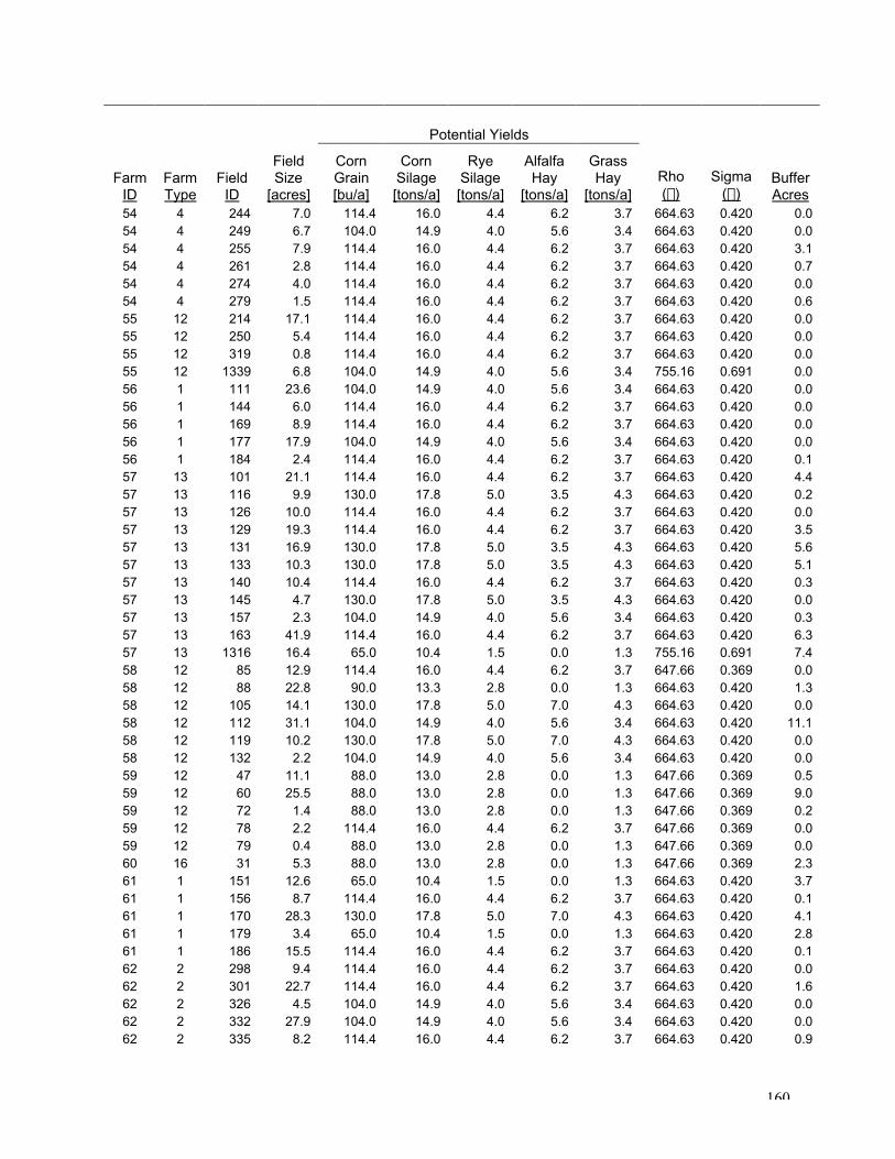
160
Potential Yields
FarmID
FarmType
FieldID
FieldSize
[acres]
CornGrain[bu/a]
CornSilage[tons/a]
RyeSilage[tons/a]
AlfalfaHay
[tons/a]
GrassHay
[tons/a]Rho(r)
Sigma(s)
BufferAcres
54 4 244 7.0 114.4 16.0 4.4 6.2 3.7 664.63 0.420 0.054 4 249 6.7 104.0 14.9 4.0 5.6 3.4 664.63 0.420 0.054 4 255 7.9 114.4 16.0 4.4 6.2 3.7 664.63 0.420 3.154 4 261 2.8 114.4 16.0 4.4 6.2 3.7 664.63 0.420 0.754 4 274 4.0 114.4 16.0 4.4 6.2 3.7 664.63 0.420 0.054 4 279 1.5 114.4 16.0 4.4 6.2 3.7 664.63 0.420 0.655 12 214 17.1 114.4 16.0 4.4 6.2 3.7 664.63 0.420 0.055 12 250 5.4 114.4 16.0 4.4 6.2 3.7 664.63 0.420 0.055 12 319 0.8 114.4 16.0 4.4 6.2 3.7 664.63 0.420 0.055 12 1339 6.8 104.0 14.9 4.0 5.6 3.4 755.16 0.691 0.056 1 111 23.6 104.0 14.9 4.0 5.6 3.4 664.63 0.420 0.056 1 144 6.0 114.4 16.0 4.4 6.2 3.7 664.63 0.420 0.056 1 169 8.9 114.4 16.0 4.4 6.2 3.7 664.63 0.420 0.056 1 177 17.9 104.0 14.9 4.0 5.6 3.4 664.63 0.420 0.056 1 184 2.4 114.4 16.0 4.4 6.2 3.7 664.63 0.420 0.157 13 101 21.1 114.4 16.0 4.4 6.2 3.7 664.63 0.420 4.457 13 116 9.9 130.0 17.8 5.0 3.5 4.3 664.63 0.420 0.257 13 126 10.0 114.4 16.0 4.4 6.2 3.7 664.63 0.420 0.057 13 129 19.3 114.4 16.0 4.4 6.2 3.7 664.63 0.420 3.557 13 131 16.9 130.0 17.8 5.0 3.5 4.3 664.63 0.420 5.657 13 133 10.3 130.0 17.8 5.0 3.5 4.3 664.63 0.420 5.157 13 140 10.4 114.4 16.0 4.4 6.2 3.7 664.63 0.420 0.357 13 145 4.7 130.0 17.8 5.0 3.5 4.3 664.63 0.420 0.057 13 157 2.3 104.0 14.9 4.0 5.6 3.4 664.63 0.420 0.357 13 163 41.9 114.4 16.0 4.4 6.2 3.7 664.63 0.420 6.357 13 1316 16.4 65.0 10.4 1.5 0.0 1.3 755.16 0.691 7.458 12 85 12.9 114.4 16.0 4.4 6.2 3.7 647.66 0.369 0.058 12 88 22.8 90.0 13.3 2.8 0.0 1.3 664.63 0.420 1.358 12 105 14.1 130.0 17.8 5.0 7.0 4.3 664.63 0.420 0.058 12 112 31.1 104.0 14.9 4.0 5.6 3.4 664.63 0.420 11.158 12 119 10.2 130.0 17.8 5.0 7.0 4.3 664.63 0.420 0.058 12 132 2.2 104.0 14.9 4.0 5.6 3.4 664.63 0.420 0.059 12 47 11.1 88.0 13.0 2.8 0.0 1.3 647.66 0.369 0.559 12 60 25.5 88.0 13.0 2.8 0.0 1.3 647.66 0.369 9.059 12 72 1.4 88.0 13.0 2.8 0.0 1.3 647.66 0.369 0.259 12 78 2.2 114.4 16.0 4.4 6.2 3.7 647.66 0.369 0.059 12 79 0.4 88.0 13.0 2.8 0.0 1.3 647.66 0.369 0.060 16 31 5.3 88.0 13.0 2.8 0.0 1.3 647.66 0.369 2.361 1 151 12.6 65.0 10.4 1.5 0.0 1.3 664.63 0.420 3.761 1 156 8.7 114.4 16.0 4.4 6.2 3.7 664.63 0.420 0.161 1 170 28.3 130.0 17.8 5.0 7.0 4.3 664.63 0.420 4.161 1 179 3.4 65.0 10.4 1.5 0.0 1.3 664.63 0.420 2.861 1 186 15.5 114.4 16.0 4.4 6.2 3.7 664.63 0.420 0.162 2 298 9.4 114.4 16.0 4.4 6.2 3.7 664.63 0.420 0.062 2 301 22.7 114.4 16.0 4.4 6.2 3.7 664.63 0.420 1.662 2 326 4.5 104.0 14.9 4.0 5.6 3.4 664.63 0.420 0.062 2 332 27.9 104.0 14.9 4.0 5.6 3.4 664.63 0.420 0.062 2 335 8.2 114.4 16.0 4.4 6.2 3.7 664.63 0.420 0.9
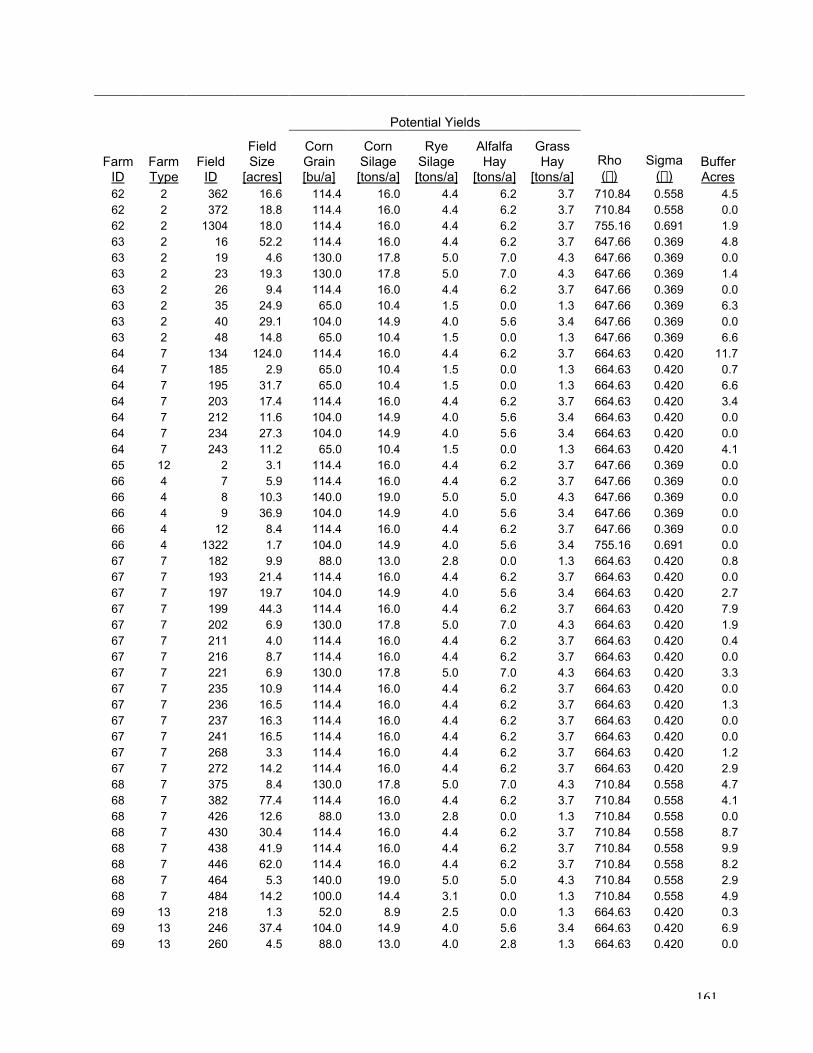
161
Potential Yields
FarmID
FarmType
FieldID
FieldSize
[acres]
CornGrain[bu/a]
CornSilage[tons/a]
RyeSilage[tons/a]
AlfalfaHay
[tons/a]
GrassHay
[tons/a]Rho(r)
Sigma(s)
BufferAcres
62 2 362 16.6 114.4 16.0 4.4 6.2 3.7 710.84 0.558 4.562 2 372 18.8 114.4 16.0 4.4 6.2 3.7 710.84 0.558 0.062 2 1304 18.0 114.4 16.0 4.4 6.2 3.7 755.16 0.691 1.963 2 16 52.2 114.4 16.0 4.4 6.2 3.7 647.66 0.369 4.863 2 19 4.6 130.0 17.8 5.0 7.0 4.3 647.66 0.369 0.063 2 23 19.3 130.0 17.8 5.0 7.0 4.3 647.66 0.369 1.463 2 26 9.4 114.4 16.0 4.4 6.2 3.7 647.66 0.369 0.063 2 35 24.9 65.0 10.4 1.5 0.0 1.3 647.66 0.369 6.363 2 40 29.1 104.0 14.9 4.0 5.6 3.4 647.66 0.369 0.063 2 48 14.8 65.0 10.4 1.5 0.0 1.3 647.66 0.369 6.664 7 134 124.0 114.4 16.0 4.4 6.2 3.7 664.63 0.420 11.764 7 185 2.9 65.0 10.4 1.5 0.0 1.3 664.63 0.420 0.764 7 195 31.7 65.0 10.4 1.5 0.0 1.3 664.63 0.420 6.664 7 203 17.4 114.4 16.0 4.4 6.2 3.7 664.63 0.420 3.464 7 212 11.6 104.0 14.9 4.0 5.6 3.4 664.63 0.420 0.064 7 234 27.3 104.0 14.9 4.0 5.6 3.4 664.63 0.420 0.064 7 243 11.2 65.0 10.4 1.5 0.0 1.3 664.63 0.420 4.165 12 2 3.1 114.4 16.0 4.4 6.2 3.7 647.66 0.369 0.066 4 7 5.9 114.4 16.0 4.4 6.2 3.7 647.66 0.369 0.066 4 8 10.3 140.0 19.0 5.0 5.0 4.3 647.66 0.369 0.066 4 9 36.9 104.0 14.9 4.0 5.6 3.4 647.66 0.369 0.066 4 12 8.4 114.4 16.0 4.4 6.2 3.7 647.66 0.369 0.066 4 1322 1.7 104.0 14.9 4.0 5.6 3.4 755.16 0.691 0.067 7 182 9.9 88.0 13.0 2.8 0.0 1.3 664.63 0.420 0.867 7 193 21.4 114.4 16.0 4.4 6.2 3.7 664.63 0.420 0.067 7 197 19.7 104.0 14.9 4.0 5.6 3.4 664.63 0.420 2.767 7 199 44.3 114.4 16.0 4.4 6.2 3.7 664.63 0.420 7.967 7 202 6.9 130.0 17.8 5.0 7.0 4.3 664.63 0.420 1.967 7 211 4.0 114.4 16.0 4.4 6.2 3.7 664.63 0.420 0.467 7 216 8.7 114.4 16.0 4.4 6.2 3.7 664.63 0.420 0.067 7 221 6.9 130.0 17.8 5.0 7.0 4.3 664.63 0.420 3.367 7 235 10.9 114.4 16.0 4.4 6.2 3.7 664.63 0.420 0.067 7 236 16.5 114.4 16.0 4.4 6.2 3.7 664.63 0.420 1.367 7 237 16.3 114.4 16.0 4.4 6.2 3.7 664.63 0.420 0.067 7 241 16.5 114.4 16.0 4.4 6.2 3.7 664.63 0.420 0.067 7 268 3.3 114.4 16.0 4.4 6.2 3.7 664.63 0.420 1.267 7 272 14.2 114.4 16.0 4.4 6.2 3.7 664.63 0.420 2.968 7 375 8.4 130.0 17.8 5.0 7.0 4.3 710.84 0.558 4.768 7 382 77.4 114.4 16.0 4.4 6.2 3.7 710.84 0.558 4.168 7 426 12.6 88.0 13.0 2.8 0.0 1.3 710.84 0.558 0.068 7 430 30.4 114.4 16.0 4.4 6.2 3.7 710.84 0.558 8.768 7 438 41.9 114.4 16.0 4.4 6.2 3.7 710.84 0.558 9.968 7 446 62.0 114.4 16.0 4.4 6.2 3.7 710.84 0.558 8.268 7 464 5.3 140.0 19.0 5.0 5.0 4.3 710.84 0.558 2.968 7 484 14.2 100.0 14.4 3.1 0.0 1.3 710.84 0.558 4.969 13 218 1.3 52.0 8.9 2.5 0.0 1.3 664.63 0.420 0.369 13 246 37.4 104.0 14.9 4.0 5.6 3.4 664.63 0.420 6.969 13 260 4.5 88.0 13.0 4.0 2.8 1.3 664.63 0.420 0.0

162
Potential Yields
FarmID
FarmType
FieldID
FieldSize
[acres]
CornGrain[bu/a]
CornSilage[tons/a]
RyeSilage[tons/a]
AlfalfaHay
[tons/a]
GrassHay
[tons/a]Rho(r)
Sigma(s)
BufferAcres
69 13 276 6.3 130.0 17.8 5.0 7.0 4.3 664.63 0.420 0.869 13 280 34.9 114.4 16.0 4.4 6.2 3.7 664.63 0.420 0.169 13 282 35.3 130.0 17.8 5.0 7.0 4.3 664.63 0.420 7.769 13 1314 60.8 114.4 16.0 4.4 6.2 3.7 755.16 0.691 4.270 17 498 8.0 65.0 10.4 1.5 0.0 1.3 710.84 0.558 3.770 17 504 17.7 65.0 10.4 1.5 0.0 1.3 710.84 0.558 7.670 17 514 10.7 104.0 14.9 4.0 5.6 3.4 710.84 0.558 0.070 17 517 13.1 114.4 16.0 4.4 6.2 3.7 710.84 0.558 0.370 17 530 16.0 65.0 10.4 1.5 0.0 1.3 710.84 0.558 3.870 17 538 5.0 114.4 16.0 4.4 6.2 3.7 710.84 0.558 0.170 17 562 5.0 114.4 16.0 4.4 6.2 3.7 710.84 0.558 2.270 17 568 16.3 114.4 16.0 4.4 6.2 3.7 710.84 0.558 0.070 17 589 9.5 65.0 10.4 1.5 0.0 1.3 710.84 0.558 5.270 17 597 29.3 104.0 14.9 4.0 5.6 3.4 710.84 0.558 7.071 12 931 2.6 88.0 13.0 2.8 0.0 1.3 755.16 0.691 0.071 12 932 7.9 88.0 13.0 2.8 0.0 1.3 755.16 0.691 0.071 12 1302 25.5 114.4 16.0 4.4 6.2 3.7 755.16 0.691 2.571 12 1325 28.0 114.4 16.0 4.4 6.2 3.7 755.16 0.691 0.072 1 1168 5.2 114.4 16.0 4.4 6.2 3.7 755.16 0.691 0.072 1 1171 4.5 104.0 14.9 4.0 5.6 3.4 755.16 0.691 0.072 1 1173 25.9 104.0 14.9 4.0 5.6 3.4 755.16 0.691 0.072 1 1174 19.8 114.4 16.0 4.4 6.2 3.7 755.16 0.691 0.072 1 1180 7.8 104.0 14.9 4.0 5.6 3.4 755.16 0.691 0.572 1 1282 14.8 0.0 0.0 0.0 0.0 1.3 755.16 0.691 2.273 17 300 29.7 65.0 10.4 1.5 0.0 1.3 664.63 0.420 12.973 17 317 37.2 114.4 16.0 4.4 6.2 3.7 664.63 0.420 1.773 17 346 29.4 114.4 16.0 4.4 6.2 3.7 710.84 0.558 2.473 17 364 12.0 114.4 16.0 4.4 6.2 3.7 710.84 0.558 0.073 17 383 5.1 114.4 16.0 4.4 6.2 3.7 710.84 0.558 0.073 17 393 5.8 114.4 16.0 4.4 6.2 3.7 710.84 0.558 0.173 17 394 8.7 65.0 10.4 1.5 0.0 1.3 710.84 0.558 3.573 17 408 3.4 114.4 16.0 4.4 6.2 3.7 710.84 0.558 0.274 17 229 18.6 130.0 17.8 5.0 7.0 4.3 664.63 0.420 0.074 17 251 71.7 114.4 16.0 4.4 6.2 3.7 664.63 0.420 22.274 17 287 16.2 65.0 10.4 1.5 0.0 1.3 664.63 0.420 6.574 17 310 2.8 114.4 16.0 4.4 6.2 3.7 664.63 0.420 0.075 17 22 14.5 114.4 16.0 4.4 6.2 3.7 647.66 0.369 0.075 17 27 21.5 65.0 10.4 1.5 0.0 1.3 647.66 0.369 7.775 17 36 1.6 65.0 10.4 1.5 0.0 1.3 647.66 0.369 0.075 17 43 12.1 88.0 13.0 2.8 0.0 1.3 647.66 0.369 6.075 17 46 16.1 114.4 16.0 4.4 6.2 3.7 647.66 0.369 0.075 17 68 6.7 100.0 14.4 3.1 0.0 1.3 647.66 0.369 1.176 12 50 17.7 88.0 13.0 2.8 0.0 1.3 647.66 0.369 1.476 12 57 19.3 114.4 16.0 4.4 6.2 3.7 647.66 0.369 0.076 12 82 8.5 130.0 17.8 5.0 7.0 4.3 647.66 0.369 1.276 12 95 17.2 130.0 17.8 5.0 7.0 4.3 664.63 0.420 3.476 12 97 13.2 130.0 17.8 5.0 3.5 4.3 664.63 0.420 0.076 12 107 2.3 130.0 17.8 5.0 3.5 4.3 664.63 0.420 0.0

163
Potential Yields
FarmID
FarmType
FieldID
FieldSize
[acres]
CornGrain[bu/a]
CornSilage[tons/a]
RyeSilage[tons/a]
AlfalfaHay
[tons/a]
GrassHay
[tons/a]Rho(r)
Sigma(s)
BufferAcres
76 12 110 1.0 130.0 17.8 5.0 7.0 4.3 664.63 0.420 0.076 12 114 15.0 130.0 17.8 5.0 7.0 4.3 664.63 0.420 1.776 12 121 1.8 114.4 16.0 4.4 6.2 3.7 664.63 0.420 0.676 12 122 3.0 130.0 17.8 5.0 7.0 4.3 664.63 0.420 0.277 17 148 59.7 104.0 14.9 4.0 5.6 3.4 664.63 0.420 0.077 17 187 51.8 114.4 16.0 4.4 6.2 3.7 664.63 0.420 6.877 17 210 3.3 104.0 14.9 4.0 5.6 3.4 664.63 0.420 0.077 17 219 13.0 104.0 14.9 4.0 5.6 3.4 664.63 0.420 0.077 17 223 3.7 104.0 14.9 4.0 5.6 3.4 664.63 0.420 0.078 1 453 31.2 0.0 0.0 0.0 0.0 1.3 710.84 0.558 0.778 1 479 22.4 104.0 14.9 4.0 5.6 3.4 710.84 0.558 0.078 1 491 2.3 104.0 14.9 4.0 5.6 3.4 710.84 0.558 0.078 1 513 3.5 114.4 16.0 4.4 6.2 3.7 710.84 0.558 0.079 1 940 9.4 117.0 16.3 4.5 6.3 3.8 755.16 0.691 0.079 1 944 8.0 114.4 16.0 4.4 6.2 3.7 755.16 0.691 0.079 1 959 9.2 117.0 16.3 4.5 6.3 3.8 755.16 0.691 0.080 7 1009 44.0 114.4 16.0 4.4 6.2 3.7 755.16 0.691 7.880 7 1029 6.3 114.4 16.0 4.4 6.2 3.7 755.16 0.691 0.080 7 1038 7.6 114.4 16.0 4.4 6.2 3.7 755.16 0.691 0.080 7 1051 3.3 114.4 16.0 4.4 6.2 3.7 755.16 0.691 0.080 7 1058 3.8 130.0 17.8 5.0 7.0 4.3 755.16 0.691 0.080 7 1059 5.9 114.4 16.0 4.4 6.2 3.7 755.16 0.691 0.080 7 1307 32.9 130.0 17.8 5.0 7.0 4.3 755.16 0.691 4.080 7 1326 43.4 114.4 16.0 4.4 6.2 3.7 755.16 0.691 0.381 17 729 7.7 55.3 9.3 2.7 0.0 1.3 710.84 0.558 0.781 17 734 14.4 96.8 14.0 4.4 3.1 1.4 710.84 0.558 0.081 17 747 7.6 130.0 17.8 5.0 7.0 4.3 710.84 0.558 0.481 17 760 2.4 130.0 17.8 5.0 7.0 4.3 710.84 0.558 0.681 17 780 1.8 130.0 17.8 5.0 7.0 4.3 710.84 0.558 0.481 17 785 0.7 130.0 17.8 5.0 7.0 4.3 710.84 0.558 0.381 17 788 3.9 130.0 17.8 5.0 7.0 4.3 710.84 0.558 1.381 17 795 2.1 96.8 14.0 4.4 3.1 1.4 710.84 0.558 0.881 17 799 5.9 96.8 14.0 4.4 3.1 1.4 710.84 0.558 0.081 17 817 3.3 96.8 14.0 4.4 3.1 1.4 710.84 0.558 0.081 17 850 2.3 100.0 14.4 3.1 0.0 1.3 710.84 0.558 0.081 17 1324 4.8 55.3 9.3 2.7 0.0 1.3 755.16 0.691 0.082 17 1124 25.3 114.4 16.0 4.4 6.2 3.7 755.16 0.691 0.682 17 1128 17.3 114.4 16.0 4.4 6.2 3.7 755.16 0.691 0.082 17 1135 39.8 114.4 16.0 4.4 6.2 3.7 755.16 0.691 10.482 17 1149 5.2 114.4 16.0 4.4 6.2 3.7 755.16 0.691 0.082 17 1156 5.8 104.0 14.9 4.0 5.6 3.4 755.16 0.691 0.082 17 1163 23.8 104.0 14.9 4.0 5.6 3.4 755.16 0.691 0.083 1 1033 18.8 114.4 16.0 4.4 6.2 3.7 755.16 0.691 0.083 1 1042 61.0 114.4 16.0 4.4 6.2 3.7 755.16 0.691 6.783 1 1054 1.3 114.4 16.0 4.4 6.2 3.7 755.16 0.691 0.083 1 1060 12.9 114.4 16.0 4.4 6.2 3.7 755.16 0.691 0.083 1 1293 8.9 65.0 10.4 1.5 0.0 1.3 755.16 0.691 4.884 17 618 92.4 104.0 14.9 4.0 5.6 3.4 710.84 0.558 11.7

164
Potential Yields
FarmID
FarmType
FieldID
FieldSize
[acres]
CornGrain[bu/a]
CornSilage[tons/a]
RyeSilage[tons/a]
AlfalfaHay
[tons/a]
GrassHay
[tons/a]Rho(r)
Sigma(s)
BufferAcres
84 17 641 1.6 65.0 10.4 1.5 0.0 1.3 710.84 0.558 1.184 17 649 5.4 65.0 10.4 1.5 0.0 1.3 710.84 0.558 3.684 17 691 20.1 104.0 14.9 4.0 5.6 3.4 710.84 0.558 0.085 17 155 4.5 114.4 16.0 4.4 6.2 3.7 664.63 0.420 0.085 17 168 9.4 114.4 16.0 4.4 6.2 3.7 664.63 0.420 0.685 17 171 3.9 114.4 16.0 4.4 6.2 3.7 664.63 0.420 0.085 17 175 4.7 104.0 14.9 4.0 5.6 3.4 664.63 0.420 0.085 17 176 35.0 104.0 14.9 4.0 5.6 3.4 664.63 0.420 6.485 17 1299 30.5 114.4 16.0 4.4 6.2 3.7 755.16 0.691 0.086 2 1178 33.1 104.0 14.9 4.0 5.6 3.4 755.16 0.691 0.286 2 1185 28.3 114.4 16.0 4.4 6.2 3.7 755.16 0.691 5.486 2 1187 8.8 114.4 16.0 4.4 6.2 3.7 755.16 0.691 0.086 2 1197 3.9 114.4 16.0 4.4 6.2 3.7 755.16 0.691 0.086 2 1200 2.1 100.0 14.4 3.1 0.0 1.3 755.16 0.691 0.086 2 1331 57.3 114.4 16.0 4.4 6.2 3.7 755.16 0.691 1.087 3 635 83.4 104.0 14.9 4.0 5.6 3.4 710.84 0.558 0.087 3 673 11.7 114.4 16.0 4.4 6.2 3.7 710.84 0.558 0.187 3 682 6.2 65.0 10.4 1.5 0.0 1.3 710.84 0.558 2.987 3 698 43.6 104.0 14.9 4.0 5.6 3.4 710.84 0.558 12.687 3 722 55.1 104.0 14.9 4.0 5.6 3.4 710.84 0.558 4.988 1 59 13.1 114.4 16.0 4.4 6.2 3.7 647.66 0.369 0.088 1 80 9.4 114.4 16.0 4.4 6.2 3.7 647.66 0.369 0.088 1 1340 4.9 104.0 14.9 4.0 5.6 3.4 755.16 0.691 0.089 17 183 17.8 114.4 16.0 4.4 6.2 3.7 664.63 0.420 0.089 17 190 14.8 140.0 19.0 5.0 5.0 4.3 664.63 0.420 0.089 17 192 6.7 130.0 17.8 5.0 7.0 4.3 664.63 0.420 0.089 17 205 7.1 104.0 14.9 4.0 5.6 3.4 664.63 0.420 2.789 17 208 17.4 130.0 17.8 5.0 7.0 4.3 664.63 0.420 0.090 4 53 35.3 114.4 16.0 4.4 6.2 3.7 647.66 0.369 0.590 4 69 9.0 65.0 10.4 1.5 0.0 1.3 647.66 0.369 2.690 4 86 14.4 130.0 17.8 5.0 7.0 4.3 664.63 0.420 4.290 4 87 8.3 114.4 16.0 4.4 6.2 3.7 664.63 0.420 0.091 17 11 6.1 114.4 16.0 4.4 6.2 3.7 647.66 0.369 0.091 17 13 18.6 114.4 16.0 4.4 6.2 3.7 647.66 0.369 2.391 17 14 7.6 114.4 16.0 4.4 6.2 3.7 647.66 0.369 0.991 17 15 8.0 130.0 17.8 5.0 7.0 4.3 647.66 0.369 0.191 17 20 5.9 130.0 17.8 5.0 7.0 4.3 647.66 0.369 2.691 17 33 0.8 114.4 16.0 4.4 6.2 3.7 647.66 0.369 0.092 12 104 7.7 130.0 17.8 5.0 7.0 4.3 664.63 0.420 2.992 12 120 9.7 100.0 14.4 3.1 0.0 1.3 664.63 0.420 3.592 12 125 19.9 100.0 14.4 3.1 0.0 1.3 664.63 0.420 4.792 12 128 19.2 114.4 16.0 4.4 6.2 3.7 664.63 0.420 1.193 1 230 31.0 114.4 16.0 4.4 6.2 3.7 664.63 0.420 0.693 1 245 3.8 104.0 14.9 4.0 5.6 3.4 664.63 0.420 0.693 1 247 24.1 65.0 10.4 1.5 0.0 1.3 664.63 0.420 10.293 1 259 14.9 104.0 14.9 4.0 5.6 3.4 664.63 0.420 0.093 1 277 10.8 114.4 16.0 4.4 6.2 3.7 664.63 0.420 0.094 12 222 5.8 104.0 14.9 4.0 5.6 3.4 664.63 0.420 0.0

165
Potential Yields
FarmID
FarmType
FieldID
FieldSize
[acres]
CornGrain[bu/a]
CornSilage[tons/a]
RyeSilage[tons/a]
AlfalfaHay
[tons/a]
GrassHay
[tons/a]Rho(r)
Sigma(s)
BufferAcres
94 12 231 8.3 104.0 14.9 4.0 5.6 3.4 664.63 0.420 0.094 12 242 5.9 104.0 14.9 4.0 5.6 3.4 664.63 0.420 0.094 12 248 5.3 104.0 14.9 4.0 5.6 3.4 664.63 0.420 0.094 12 253 9.1 114.4 16.0 4.4 6.2 3.7 664.63 0.420 0.094 12 254 4.0 114.4 16.0 4.4 6.2 3.7 664.63 0.420 0.094 12 269 13.0 114.4 16.0 4.4 6.2 3.7 664.63 0.420 3.594 12 283 18.7 104.0 14.9 4.0 5.6 3.4 664.63 0.420 0.094 12 285 3.3 114.4 16.0 4.4 6.2 3.7 664.63 0.420 0.094 12 294 12.2 114.4 16.0 4.4 6.2 3.7 664.63 0.420 4.395 17 356 8.6 114.4 16.0 4.4 6.2 3.7 710.84 0.558 0.895 17 359 4.5 104.0 14.9 4.0 5.6 3.4 710.84 0.558 0.095 17 368 3.2 104.0 14.9 4.0 5.6 3.4 710.84 0.558 0.095 17 378 7.2 104.0 14.9 4.0 5.6 3.4 710.84 0.558 0.095 17 392 1.0 104.0 14.9 4.0 5.6 3.4 710.84 0.558 0.095 17 405 3.5 114.4 16.0 4.4 6.2 3.7 710.84 0.558 0.095 17 415 1.4 114.4 16.0 4.4 6.2 3.7 710.84 0.558 0.095 17 418 10.8 114.4 16.0 4.4 6.2 3.7 710.84 0.558 0.096 12 516 4.1 104.0 14.9 4.0 5.6 3.4 710.84 0.558 0.096 12 519 1.8 114.4 16.0 4.4 6.2 3.7 710.84 0.558 0.096 12 523 6.4 104.0 14.9 4.0 5.6 3.4 710.84 0.558 0.496 12 540 7.0 104.0 14.9 4.0 5.6 3.4 710.84 0.558 1.696 12 548 28.3 104.0 14.9 4.0 5.6 3.4 710.84 0.558 3.496 12 577 20.6 104.0 14.9 4.0 5.6 3.4 710.84 0.558 0.096 12 586 8.0 114.4 16.0 4.4 6.2 3.7 710.84 0.558 0.096 12 1336 4.6 104.0 14.9 4.0 5.6 3.4 755.16 0.691 0.097 12 560 7.8 114.4 16.0 4.4 6.2 3.7 710.84 0.558 0.097 12 566 15.5 114.4 16.0 4.4 6.2 3.7 710.84 0.558 0.097 12 581 8.8 130.0 17.8 5.0 5.0 4.3 710.84 0.558 0.197 12 587 6.1 114.4 16.0 4.4 6.2 3.7 710.84 0.558 0.097 12 603 29.3 130.0 17.8 5.0 5.0 4.3 710.84 0.558 2.697 12 622 7.7 65.0 10.4 1.5 0.0 1.3 710.84 0.558 4.098 1 490 28.4 114.4 16.0 4.4 6.2 3.7 710.84 0.558 0.198 1 545 17.1 114.4 16.0 4.4 6.2 3.7 710.84 0.558 1.299 1 528 24.1 104.0 14.9 4.0 5.6 3.4 710.84 0.558 2.7100 2 463 14.4 114.4 16.0 4.4 6.2 3.7 710.84 0.558 0.4100 2 465 35.9 104.0 14.9 4.0 5.6 3.4 710.84 0.558 2.6100 2 481 28.8 114.4 16.0 4.4 6.2 3.7 710.84 0.558 0.0100 2 520 4.7 114.4 16.0 4.4 6.2 3.7 710.84 0.558 0.0100 2 531 8.4 114.4 16.0 4.4 6.2 3.7 710.84 0.558 0.0100 2 533 12.4 114.4 16.0 4.4 6.2 3.7 710.84 0.558 0.0100 2 537 29.5 130.0 17.8 5.0 7.0 4.3 710.84 0.558 0.0101 17 694 24.6 72.3 11.2 4.3 0.0 1.3 710.84 0.558 8.4101 17 708 5.6 72.3 11.2 4.3 0.0 1.3 710.84 0.558 2.7101 17 709 13.4 114.4 16.0 4.4 6.2 3.7 710.84 0.558 3.9101 17 736 16.3 104.0 14.9 4.0 5.6 3.4 710.84 0.558 4.8101 17 1289 55.4 114.4 16.0 4.4 6.2 3.7 755.16 0.691 4.2102 17 626 10.9 130.0 17.8 5.0 7.0 4.3 710.84 0.558 2.3102 17 675 3.7 114.4 16.0 4.4 6.2 3.7 710.84 0.558 0.2
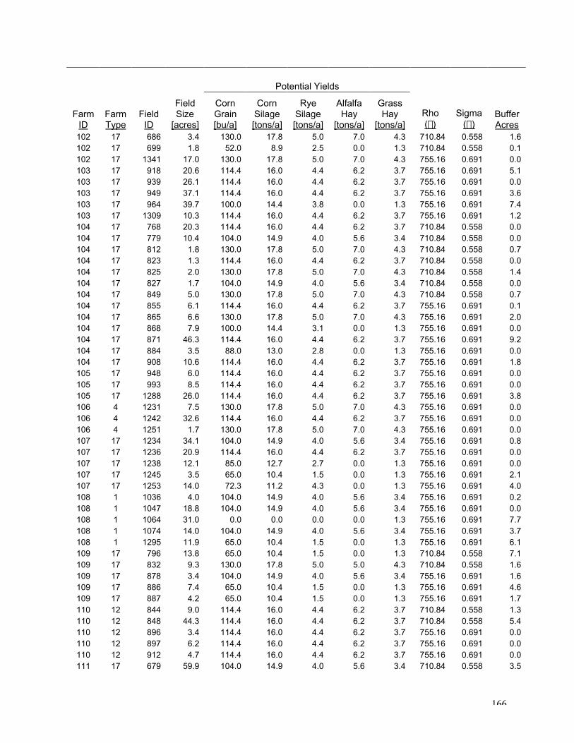
166
Potential Yields
FarmID
FarmType
FieldID
FieldSize
[acres]
CornGrain[bu/a]
CornSilage[tons/a]
RyeSilage[tons/a]
AlfalfaHay
[tons/a]
GrassHay
[tons/a]Rho(r)
Sigma(s)
BufferAcres
102 17 686 3.4 130.0 17.8 5.0 7.0 4.3 710.84 0.558 1.6102 17 699 1.8 52.0 8.9 2.5 0.0 1.3 710.84 0.558 0.1102 17 1341 17.0 130.0 17.8 5.0 7.0 4.3 755.16 0.691 0.0103 17 918 20.6 114.4 16.0 4.4 6.2 3.7 755.16 0.691 5.1103 17 939 26.1 114.4 16.0 4.4 6.2 3.7 755.16 0.691 0.0103 17 949 37.1 114.4 16.0 4.4 6.2 3.7 755.16 0.691 3.6103 17 964 39.7 100.0 14.4 3.8 0.0 1.3 755.16 0.691 7.4103 17 1309 10.3 114.4 16.0 4.4 6.2 3.7 755.16 0.691 1.2104 17 768 20.3 114.4 16.0 4.4 6.2 3.7 710.84 0.558 0.0104 17 779 10.4 104.0 14.9 4.0 5.6 3.4 710.84 0.558 0.0104 17 812 1.8 130.0 17.8 5.0 7.0 4.3 710.84 0.558 0.7104 17 823 1.3 114.4 16.0 4.4 6.2 3.7 710.84 0.558 0.0104 17 825 2.0 130.0 17.8 5.0 7.0 4.3 710.84 0.558 1.4104 17 827 1.7 104.0 14.9 4.0 5.6 3.4 710.84 0.558 0.0104 17 849 5.0 130.0 17.8 5.0 7.0 4.3 710.84 0.558 0.7104 17 855 6.1 114.4 16.0 4.4 6.2 3.7 755.16 0.691 0.1104 17 865 6.6 130.0 17.8 5.0 7.0 4.3 755.16 0.691 2.0104 17 868 7.9 100.0 14.4 3.1 0.0 1.3 755.16 0.691 0.0104 17 871 46.3 114.4 16.0 4.4 6.2 3.7 755.16 0.691 9.2104 17 884 3.5 88.0 13.0 2.8 0.0 1.3 755.16 0.691 0.0104 17 908 10.6 114.4 16.0 4.4 6.2 3.7 755.16 0.691 1.8105 17 948 6.0 114.4 16.0 4.4 6.2 3.7 755.16 0.691 0.0105 17 993 8.5 114.4 16.0 4.4 6.2 3.7 755.16 0.691 0.0105 17 1288 26.0 114.4 16.0 4.4 6.2 3.7 755.16 0.691 3.8106 4 1231 7.5 130.0 17.8 5.0 7.0 4.3 755.16 0.691 0.0106 4 1242 32.6 114.4 16.0 4.4 6.2 3.7 755.16 0.691 0.0106 4 1251 1.7 130.0 17.8 5.0 7.0 4.3 755.16 0.691 0.0107 17 1234 34.1 104.0 14.9 4.0 5.6 3.4 755.16 0.691 0.8107 17 1236 20.9 114.4 16.0 4.4 6.2 3.7 755.16 0.691 0.0107 17 1238 12.1 85.0 12.7 2.7 0.0 1.3 755.16 0.691 0.0107 17 1245 3.5 65.0 10.4 1.5 0.0 1.3 755.16 0.691 2.1107 17 1253 14.0 72.3 11.2 4.3 0.0 1.3 755.16 0.691 4.0108 1 1036 4.0 104.0 14.9 4.0 5.6 3.4 755.16 0.691 0.2108 1 1047 18.8 104.0 14.9 4.0 5.6 3.4 755.16 0.691 0.0108 1 1064 31.0 0.0 0.0 0.0 0.0 1.3 755.16 0.691 7.7108 1 1074 14.0 104.0 14.9 4.0 5.6 3.4 755.16 0.691 3.7108 1 1295 11.9 65.0 10.4 1.5 0.0 1.3 755.16 0.691 6.1109 17 796 13.8 65.0 10.4 1.5 0.0 1.3 710.84 0.558 7.1109 17 832 9.3 130.0 17.8 5.0 5.0 4.3 710.84 0.558 1.6109 17 878 3.4 104.0 14.9 4.0 5.6 3.4 755.16 0.691 1.6109 17 886 7.4 65.0 10.4 1.5 0.0 1.3 755.16 0.691 4.6109 17 887 4.2 65.0 10.4 1.5 0.0 1.3 755.16 0.691 1.7110 12 844 9.0 114.4 16.0 4.4 6.2 3.7 710.84 0.558 1.3110 12 848 44.3 114.4 16.0 4.4 6.2 3.7 710.84 0.558 5.4110 12 896 3.4 114.4 16.0 4.4 6.2 3.7 755.16 0.691 0.0110 12 897 6.2 114.4 16.0 4.4 6.2 3.7 755.16 0.691 0.0110 12 912 4.7 114.4 16.0 4.4 6.2 3.7 755.16 0.691 0.0111 17 679 59.9 104.0 14.9 4.0 5.6 3.4 710.84 0.558 3.5

167
Potential Yields
FarmID
FarmType
FieldID
FieldSize
[acres]
CornGrain[bu/a]
CornSilage[tons/a]
RyeSilage[tons/a]
AlfalfaHay
[tons/a]
GrassHay
[tons/a]Rho(r)
Sigma(s)
BufferAcres
111 17 693 24.9 104.0 14.9 4.0 5.6 3.4 710.84 0.558 0.0111 17 704 23.0 114.4 16.0 4.4 6.2 3.7 710.84 0.558 0.0111 17 725 8.3 65.0 10.4 1.5 0.0 1.3 710.84 0.558 7.0111 17 732 13.4 114.4 16.0 4.4 6.2 3.7 710.84 0.558 0.0112 4 610 11.7 104.0 14.9 4.0 5.6 3.4 710.84 0.558 0.0112 4 637 8.9 104.0 14.9 4.0 5.6 3.4 710.84 0.558 0.0112 4 657 23.8 130.0 17.8 5.0 3.5 4.3 710.84 0.558 4.3113 17 1284 96.8 104.0 14.9 4.0 5.6 3.4 755.16 0.691 24.4114 17 1016 10.0 114.4 16.0 4.4 6.2 3.7 755.16 0.691 0.0114 17 1306 14.3 100.0 14.4 3.1 0.0 1.3 755.16 0.691 4.0114 17 1308 35.1 114.4 16.0 4.4 6.2 3.7 755.16 0.691 10.5115 4 1138 8.9 114.4 16.0 4.4 6.2 3.7 755.16 0.691 0.4115 4 1310 11.9 114.4 16.0 4.4 6.2 3.7 755.16 0.691 0.0116 12 1312 55.2 114.4 16.0 4.4 6.2 3.7 755.16 0.691 10.2117 17 1286 73.9 104.0 14.9 4.0 5.6 3.4 755.16 0.691 14.1118 17 428 18.9 114.4 16.0 4.4 6.2 3.7 710.84 0.558 0.6118 17 443 15.7 114.4 16.0 4.4 6.2 3.7 710.84 0.558 5.6118 17 467 7.5 114.4 16.0 4.4 6.2 3.7 710.84 0.558 0.0118 17 482 8.6 114.4 16.0 4.4 6.2 3.7 710.84 0.558 0.0118 17 1315 11.2 114.4 16.0 4.4 6.2 3.7 755.16 0.691 4.9119 12 141 14.4 104.0 14.9 4.0 5.6 3.4 664.63 0.420 0.0119 12 162 6.4 114.4 16.0 4.4 6.2 3.7 664.63 0.420 0.0119 12 167 14.7 114.4 16.0 4.4 6.2 3.7 664.63 0.420 1.5119 12 180 5.6 114.4 16.0 4.4 6.2 3.7 664.63 0.420 0.3119 12 188 6.2 130.0 17.8 5.0 7.0 4.3 664.63 0.420 1.7120 17 77 8.1 104.0 14.9 4.0 5.6 3.4 647.66 0.369 0.0120 17 83 19.7 114.4 16.0 4.4 6.2 3.7 647.66 0.369 4.7120 17 103 16.1 114.4 16.0 4.4 6.2 3.7 664.63 0.420 0.0120 17 106 4.1 114.4 16.0 4.4 6.2 3.7 664.63 0.420 0.0120 17 109 10.2 104.0 14.9 4.0 5.6 3.4 664.63 0.420 0.0120 17 117 11.1 114.4 16.0 4.4 6.2 3.7 664.63 0.420 4.8120 17 123 11.7 104.0 14.9 4.0 5.6 3.4 664.63 0.420 0.0120 17 135 13.2 104.0 14.9 4.0 5.6 3.4 664.63 0.420 0.0121 17 39 3.0 114.4 16.0 4.4 6.2 3.7 647.66 0.369 0.0121 17 41 8.3 114.4 16.0 4.4 6.2 3.7 647.66 0.369 0.0121 17 45 0.7 114.4 16.0 4.4 6.2 3.7 647.66 0.369 0.0121 17 49 7.0 114.4 16.0 4.4 6.2 3.7 647.66 0.369 0.0121 17 55 20.6 114.4 16.0 4.4 6.2 3.7 647.66 0.369 2.1

168
Vita
JOHN G. BONHAMRR 1 Box 269J 540.544.7817Newport, VA 24128 [email protected]
Education:2003 M.S. – Agricultural and Applied Economics
Virginia Polytechnic Institute and State University; Blacksburg, Virginia3.47 GPA Microeconomic Theory, Macroeconomic Theory, Econometrics, Mathematics,
Math Programming, Rural Development, Risk Analysis, Environmental & ResourceEconomics
1994 B.S. – Business AdministrationCollege of Charleston; Charleston, South Carolina
Professional Experience:August, 2000 – July, 2003 Research AssistantDepartment of Agricultural and Applied Economics; Virginia Tech; Blacksburg, VA
My research involves policies that are designed to improve water quality by reducing thequantity of nutrient runoff from agriculture. The goal is to evaluate how spatial informationimproves the accuracy of estimates of economic and physical responses to policies that seek tocontrol NPS pollution from agriculture. Specifically, the objective is to estimate the accuracy ofpredicted compliance costs and phosphorous reductions of two design standards under threealternative levels of information relative to the population. A linear programming model isincorporated with a GIS and the Virginia P-Index. Through modeling I am able to estimate howfarmers will react to, and be effected by, imposed regulations. This research has includedinterdisciplinary work with graduate students and professors, and government agents. I haveconducted literature reviews and have become familiar with agriculture, soils and nutrients, andhydrology.
August 1999 – June 2000 Finance AssistantAmerican Red Cross; Washington, D.C.Analyzed budgets and expenses, and prepared reports for management and donors for theKosovo Crisis Relief Program. Designed an expense tracking and reporting system in Excel forthe multi-project program.

169
November 1996 – June 1998 Mutual Fund Accounting Analyst/SupervisorSEI Investments; Oaks, PennsylvaniaCalculated/reviewed net asset value and income distribution of multiple mutual and moneymarket funds and prepared their financial statements; created tools that linked Excel and theaccounting system to improve the efficiency and accuracy of daily yield calculations; proposedand implemented changes that improved daily procedures. Selected for a pilot team thatsuccessfully integrated two accounting groups; selected for a new, high-profile client team;received the Above and Beyond Award; was promoted from analyst to supervisor.
Software Applications:MS Excel; GAMS (General Algebraic Modeling System); ESRI ArcView GIS (workingknowledge)