effects of rubber shock absorber on the flywheel micro

PHOTONIC SENSORS / Vol. 6, No. 4, 2016: 372–384

Effects of Rubber Shock Absorber on the Flywheel Micro Vibration in the Satellite Imaging System

Changcheng DENG1,2, Deqiang MU1,3, Xuezhi JIA1, and Zongxuan LI1

1National & Local United Engineering Research Center of Small Satellite Technology, Changchun Institute of Optics,

Fine Mechanics, and Physics ,Chinese Academy of Sciences, Changchun, 130033, China 2University of Chinese Academy of Sciences, Beijing, 100039, China 3Changchun University of Technology, Changchun, 130012, China *Corresponding author: Changcheng DENG E-mail: [email protected]

Abstract: When a satellite is in orbit, its flywheel will generate micro vibration and affect the imaging quality of the camera. In order to reduce this effect, a rubber shock absorber is used, and a numerical model and an experimental setup are developed to investigate its effect on the micro vibration in the study. An integrated model is developed for the system, and a ray tracing method is used in the modeling. The spot coordinates and displacements of the image plane are obtained, and the modulate transfer function (MTF) of the system is calculated. A satellite including a rubber shock absorber is designed, and the experiments are carried out. Both simulation and experiments results show that the MTF increases almost 10 %, suggesting the rubber shock absorber is useful to decrease the flywheel vibration.

Keywords: Micro vibration; flywheel; rubber shock absorber; integrated modeling; MTF; isolation experiment

Citation: Changcheng DENG, Deqiang MU, Xuezhi JIA, and Zongxuan LI, “Effects of Rubber Shock Absorber on the FlywheelMicro Vibration in the Satellite Imaging System,” Photonic Sensors, 2016, 6(4): 372–384.

1. Introduction

During photographing of the in-orbit satellite, all

kinds of motion of the moving components of the

satellite, such as the rotation of the reaction flywheel,

the jet of the propulsor, and the adjustment of solar

panels, will cause the jitter response of the camera,

thus affecting the image quality. The jitter response,

also called the micro vibration system, cannot be

measured and controlled by the attitude control

system [1]. The rotation of the flywheel will have a

relatively large impact on the image quality and is a

main issue on the satellite imaging system [2].

To reduce the influence of micro vibration on

imaging, different types of vibration control

technologies are used [3], namely as passive and

active vibration isolations, vibration absorption,

vibration resistance, and dynamic designs. Among

them, the vibration isolation method is most widely

used. The principle of the vibration isolation method

is adding a resilient liner (such as spring, rubber

mats, and blankets) between the object and the

supporting surface to isolate the vibration [4‒6].

A rubber shock absorber [7] has the advantages

of compact structure, low cost, good craftwork, etc.,

which is a very common passive vibration isolator

and often used in many fields such as ships,

buildings, and bridges. It is also easy to fabricate

and meet the required stiffness and strength. Its

Received: 24 May 2016 / Revised: 16 June 2016 © The Author(s) 2016. This article is published with open access at Springerlink.com DOI: 10.1007/s13320-016-0349-1 Article type: Regular

Changcheng DENG et al.: Effects of Rubber Shock Absorber on the Flywheel Micro Vibration in the Satellite Imaging System

373

damping ratio is 0.06 ‒ 0.1 and can absorb

mechanical energy, especially high frequency

mechanical energy. It can be bonded with metal,

forming a multilayered structure to bear load, reduce

system stiffness, and change its frequency range. A

review on the application of the rubber shock

absorber in aerospace can be found in [8]. An

accurate and efficient finite element modeling [9]

and static characteristics analysis of the rubber

shock absorber was proposed by Haiting [12].

Sjoberg investigated rubber shock absorber dynamic

modeling and dynamic characteristics [13]. Sjoberg

used the method of fractional derivative to establish

a simulation model [14]. In this study, a rubber

shock absorber is added in the flywheel system to

reduce the micro vibration of a satellite imaging

system.

The principle of the integrated modeling is to

integrate the analysis of the overall system,

containing realistic structures, disturbance, optics

and controls models, and their mutual interactions

[15–17]. It is convenient for electronic transfer of

data among all types of analysis, and this method

can save operating time, heighten analyzing qualities,

and achieve a dynamic front-to-end analysis of the

disturbance to performance paths within the satellite.

Compared with the traditional design and

assessment methods that focus on single machine or

single discipline or sub system level, integrated

modeling can provide a systematic and

comprehensive performance evaluation and error

analysis, and guide systemic design. The ray tracing

is used to calculate the location and direction of the

output ray, and the angle between the ray and the

optical axis. The calculation is based on the

reflection lens displacement and the incident light,

according to the refraction law. In this paper, the ray

tracing method is used in the integrated modeling to

analyze the influence of micro vibration on the

satellite image.

An experiment is designed to use real products

to verify the influence rubber shock absorber on the

micro vibration of the flywheel in the satellite

imaging system [18]. The data of vibration are

obtained by the ground image acquisition and

processing system, and the corresponding

performance values are calculated. The results show

that the rubber shock absorber can reduce the

vibration in the transfer path and give out better

image, which provides a guideline for the satellite

design.

2. Integrated modeling of the satellite

The integrated modeling of the satellite consists

of the modeling of the flywheel characteristic of

vibration, the finite element modeling of the entire

satellite platform, and the optical modeling based on

ray tracing [19]. The process is shown in Fig. 1.

Finite element model of the entire

satellite

Displacement of lenses of

camera

Descending of transfer function

Flywheel characteristic Of vibration

Analysis of

normal modeAnalysis of transience

responseRay trace

optical

modeling

Flywheel characteristic of

vibration

Analysis of normal mode Analysis of transience response

Ray trace

Finite element model of the

entire satellite Displacement of lenses of camera

Optical modeling

Descending of transfer function

Fig. 1 Schematic of the integrated modeling.

Photonic Sensors

374

2.1 Modeling of flywheel characteristic of vibration

The micro vibration of the flywheel is caused by

static unbalance and dynamic unbalance of the

flywheel [20], as shown in Fig. 2. The static

unbalance is caused by the deviation of the center of

mass of the flywheel rotor from its rotating axis, and

the flywheel can be considered as a rotor with two

parts, the strict rotational symmetry part and a mass

point ms part at a distance of rs from the flywheel

shaft line. Fr is the rotor inertia force. Dynamic

unbalance refers to the uneven distribution of rotor

mass which causes the cross product of inertia not

zero. The rotor can be considered as two parts, a

strict symmetry section part and 2 mass points md

part at a distance of h in the axial direction. The

mass point is at a distance rd from the rotating axis.

When the rotor rotates, the mass point ms in

static imbalance is subjected to the radial force: 2

r sF U (1)

where s s s

U m r is a flywheel mass property, and

is the angular velocity.

rs ms

Fr

(a)

h

md

rd

ex

ey ez

(b)

Fig. 2 Schematic of two types of the unbalanced flywheel [17]: (a) static unbalanced flywheel and (b) dynamic unbalanced flywheel.

For the dynamic unbalanced flywheel, the force

caused by the moment of two mass points md is 2

dT U (2) where

d d dU m r h is a dynamic unbalance property.

2.2 Finite element model of the entire satellite

The finite element structure model is the basis of

dynamic analysis (including the following modal

analysis and transient analysis). The dynamics of a

multi-degree-of-freedom system (structure) are

described in the time domain by the equation [21]: x x x M C K F (3)

where M, C, and K are N×N dimensional matrices,

of which M is the mass matrix, C is the damping

matrix, and K is the stiffness matrix; F is the force

matrix; x is the displacement response. Introducing

physical modal transformation =x qΦ (Φ is the

N×N matrix of the modal shape, q is for the modal

coordinates). Equation (3) can be decoupled as the

modal space equation: 22 Tq q q ΖΩ Ω Φ F . (4)

Supposing retained r modes (three rigid translational

modes are not considered), q rR is modal

coordinates; rxrZ R is the diagonal damping

matrix; nxrΦ R is the mass normalized modal

matrix; rxrΩ R is the natural frequency of the

diagonal matrix. Equation (5) is the transformed

equation to state-space equation of (4):

p pp w u

z zw zu

y yw yu

x x

z w

y u

A B B

C D D

C D D

(5)

where xp [ , ]T= q q , ,w u F , w wnR , u unR , w

is the disturbance input, and u is the control

input; z znR is the response output of the

satellite; y ynR is the control measure output. The

system matrix is 0 00

2

0 0

0 0

T Tw up w u

z zw zu z

y yw yu y

2

I

Φ β Φ βΩ ZA B B

C D D = Φβ

C D D Φβ

(6)


375

where wβ , uβ , zβ , and yβ are the modal

selection matrices.

Parameters of the camera in the modeling are:

focus f = 8 mm; F# (F-number) = 13.3; wavelength

500 nm ‒ 800 nm. The finite element modeling of the

satellite is completed by Patran/Nastran MSC

software. The satellite model has 33893 nodes and

21856 elements. The model is used for the following

simulation analysis to obtain displacements of all

lenses. There is no displacement constrain in the

model.

2.3 Ray tracing

The positions of the misaligned lenses are

obtained after the vibration, and an optical path

transmission is modeled with the ray tracing method

in the study. By using kinematic concepts, the

position of each lens is described with two

coordinate systems, which are the lens coordinate

system omxmymzm and the implicated coordinate

system oxyz. When the optical system is not subject

to vibration, the lens coordinate system and

implicated coordinate system are identical, and this

is in the ideal position. When the vibration occurs,

the lens coordinate system diverts from the

implicated coordinate system. The lens coordinate

system follows the lens, and the implicated

coordinate system follows the base. Supposing the

light transfers in reflection and the misaligned lens

is parabolic, the misaligned lens is explained

by an equation of lens in the lens coordinate, which

is 2 22 .m m mpz x y (7)

The optical path transmission is based on the

implicated coordinate. The equation of the

misaligned lens relative to the implicated coordinate

system is obtained by twice rotation and once

translation of coordinates. Two points are taken from

the center of up and low surfaces as shown in Fig. 3,

i.e., Points 1 and 2, so the connection line of Points

1 and 2 is the optical axis, which can describe the

displacement of the lens. Point 1 is the origin of the

lens coordinate system, and the connecting direction

of the two points is the zm direction of the coordinate

axis. When Point 1 and the connecting direction of

the line are determined, the position of the

misaligned lens can be obtained. Because a

parabolic surface is rotated, there is no need to

consider the rotation of the lens.

Point 2

Point 1

Fig. 3 Key points of lens.

The equation of the misaligned lens can be

calculated as in [22]:

1 1

1 1 1

2 21 1 1

( , , ) 2 (( )sin cos (( )cos

( )sin )) (( )cos sin (( )cos

( )sin )) (( )cos ( )sin )

0

F x y z p x x z z

y y x x z z

y y y y z z

(8)

where α is the angle rotated around axis x of

coordinate oxyz, to receive coordinate ox’y’z’;

β is the angle rotated around axis y’ of coordinate

ox’y’z’, to receive coordinate ox”y”z”, as shown

in Fig. 4; (Δx1, Δy1, Δz1) is the misaligned

displacement of Point 1; (Δx2, Δy2, Δz2)

is the misaligned displacement of Point 2.

Assuming

2 1

2 1

2 1,

a x x

b y x

c z x

(9)

then

2 2

2 2 2

sin

sin .

b

b ca

a b c

(10)

Photonic Sensors

376

Fig. 4 Rotation of the coordinate system.

The ray tracing method for a single misaligned

reflector application is shown in Fig. 5. When the

displacements of Points 1 and 2 and the incident ray

equation are given, the Matlab solving function is

used to obtain the intersection between the

misaligned lens and the incident ray. The vector in

the direction of the light reflection is calculated by

the vector reflection law, thus the angle between the

reflection light and the optical axis is obtained.

Projection of

reflection ray on xy plane

x

o

y

z

Misaligned mirror

Incident ray

Normal

Reflection ray

Fig. 5 Ray reflected by the misaligned lens.

The procedures of the ray tracing method for

modeling a single misaligned lens optical

transmission path are as follows:

(1) Obtain the equation of the misaligned lens

by the coordinate transform ( , , ) 0F x y z .

(2) Calculate the intersection between the

incident ray and misaligned lens, and the equation of

the incident ray is

1 1 1c c c

x y z

x x y y z z

I I I

(11)

where I=Ix, Iy, Iz is the vector of the incident ray. (3) Obtain the normal vector

, , x x z

F F F

N of the intersection (xc, yc, zc), and

N is normalized by the equation N

nN

.

(4) Calculate the direction vector 2 ( ) R = I n n I [23] of the reflected ray by the

reflection equation in vectors, where R=Rx, Ry, Rz

is the vector of the reflected ray, n is the normalized

vector of the lens at the intersection, and the

equation of the reflected ray is

.c c c

x y z

x x y y z z

R R R

(12)

(5) Obtain the angle between the reflected ray

and optic axis, arccos z

z

R n

R n, where nz =

0, 0, ‒1. Because the reflected light is downward, the

angle between the vertical downward direction and

reflected ray can be acquired. The reflected ray is

projected to the xy plane, and then the angle γ

between the projection line and x axis is obtained.

When the ray tracing method is applied to the plural

misaligned lens, the above five steps will be applied

to each misaligned lens in turn.

3. Design of rubber shock absorber

Only one flywheel is used in the study, which

has a total mass of 3.585 kg including four screws on

the bracket (the mass of the bracket is 1.11 kg). It is

installed on the y load plate, and each screw is

mounted with a rubber shock absorber, as shown in

Fig. 6.

The limit static stress of the rubber shock

absorber can be calculated as follows: '

'

F

S (13)

where F′ is the static load of the shock absorber; S′


377

is the minimum bearing area of the shock absorber.

For the low damping material, is 1.8 MPa, thus the

minimum area S′ of the shock absorber is 6.39 mm2

for a static load of 11.5 N. The screw is M5 then

[24].

The Y load py load plate

Fig. 6 Rubber shock absorber.

The natural frequency of the shock absorber fn is

1

2n

K gf

G

(14)

where K′ is the dynamic stiffness of the shock

absorber; g is the acceleration of gravity; G is the

gravity of the shock absorber. According to technical

indicators on the satellite equipment, the vibration

frequency ranges are from 10 Hz to 2000 Hz. If the

vibration frequency meets 2 nf f (suppose its

natural frequency fn = 10 Hz), rubber shock absorber

damping takes effect, and the total dynamic stiffness

calculated by (14) is K′ = 18516.33 N/m.

The complex shape of the shock absorber should

be taken into account as a result of the parallel and

series connection of some simple shapes. Thus the

total rigidity of the connection is written as

1 2c c ck k k (15)

1 2

1 1 1.

b b bk k k

(16)

For easy calculation, the stress-strain

relationship of the rubber damper is linear, then

cS

SEK

h (17)

where KS is the static stiffness of the shock absorber,

and '

S

K

Kis generally 1.2 ‒ 2; S is the effective load

area of the shock absorber; Ec is the effective compression modulus of shock absorber; h is the height of the shock absorber.

The effective compression modulus can be

expressed mathematically as 2

0 (1 2 '' )cE E K C (18) where E0 is the elastic modulus of rubber materials; C is a shape factor of the rubber shock absorber, which is the ratio between the loaded area and not

loaded area, and can be calculated by 4 '

DC

h ,

where D is the diameter, and h′ is the height of the shock absorber. To ensure the stability of the shock

absorber, not bending, the condition '

1h

D is

required; K′′ is the correction factor of the material properties, which ranges from 0.5 to 1.

Assuming '

1.5S

K

K , then the total stiffness is

KS = 12344.22 N/m. Supposing four shock absorbers

bear the load uniformly, the static stiffness of each

shock absorber is K′S= 3086.05 N/m according to

(15); the effective compression modulus of each

shock absorber is Ec= 0.163 MPa according to (17);

the elastic modulus of the damper material is E0 =

108.67 kPa according to (18) and the shock absorber

structure size (as shown in Fig. 7). The elastic

modulus of the rubber is about 100 kPa, so it can be

used [25].

The rubber is made in 703 Institute, and the

damping ratio of the rubber shock absorber is 0.1.

The dimension of the rubber shock absorber is used

in the following simulation and experimental design.

6

3

12

5.1

8

Fig. 7 Structure of the rubber shock absorber.

4. Vibration simulation analysis

4.1 Modal analysis

Modal analysis is to determine the dynamic

characteristics of the camera, which provides given

Photonic Sensors

378

order natural frequencies and mode shapes,

investigate the dynamic stiffness of the camera, and

assess its other dynamic performances [26]. This is

the basis of other dynamic response analyses

(such as transient analysis). From the modal

analysis, the weakness of structural rigidity is

obtained which is used for the design optimization.

The first few modals and shapes of the entire

satellite are shown in Table 1. The modal is low, but

it meets the design. The coordinate system is that the

optical axis is z axis, which consists of axes x, y,

and z, and follows the right-handed coordinate

system.

Table 1 Modal and shapes.

Modal order Frequency (Hz) Shapes

1 15.93 Swinging about yz plane

2 17.242 Swinging about xz plane

3 30.618 Twisting about z axis

5 35.694 Swinging about xy plane

4.2 Transient analysis

The static and dynamic unbalanced forces and

moments are tested by the HR-FP3402 force

platform as shown in Fig. 8(a). Figures 8 (b) and 8(c)

show an example of the force results (at the speed of

3000 rpm) for the flywheel without and with

isolation.

Flywheel

Electric wire

HR-FP3402 force platfor

Flywheel

Electric wire

HR FP3402force platform

(a)

Time(s)

Fy(N

)

Time (s)25

20

15

10

5

Fy (

N)

0

5

10

(b)

(c)

Fig. 8 Test platform and tested force results of the flywheel: (a) test platform for the force and moment of the flywheel, (b) test result Fy of the flywheel without isolation, and (c) test result Fy of the flywheel with isolation.


379

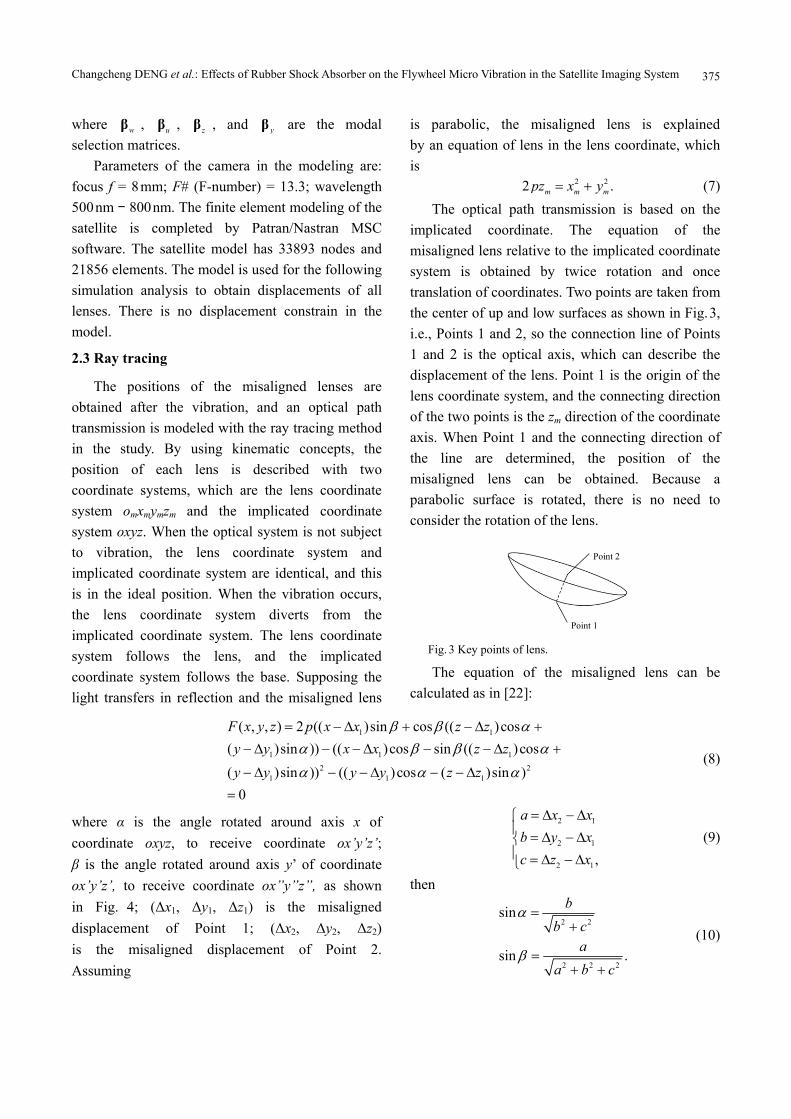
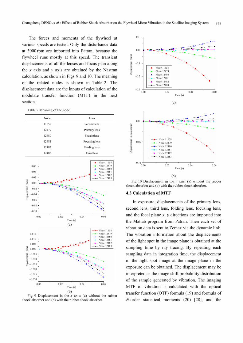
The forces and moments of the flywheel at

various speeds are tested. Only the disturbance data

at 3000 rpm are imported into Patran, because the

flywheel runs mostly at this speed. The transient

displacements of all the lenses and focus plan along

the x axis and y axis are obtained by the Nastran

calculation, as shown in Figs. 9 and 10. The meaning

of the related nodes is shown in Table 2. The

displacement data are the inputs of calculation of the

modulate transfer function (MTF) in the next

section.

Table 2 Meaning of the node.

Node Lens

11658 Second lens

12479 Primary lens

12480 Focal plane

12481 Focusing lens

12482 Folding lens

12483 Third lens

0.00 0.02 0.04 0.06Time (s)

0.10

0.06

0.04

0.00

0.02

0.04

0.06

Dis

palc

emen

t (m

m)

0.02

0.08

Node 11658Node 12479Node 12480Node 12481Node 12482Node 12483

(a)

0.00 0.02 0.04 0.06Time (s)

0.025

0.015

0.010

0.000

0.005

0.010

0.015

Dis

palc

emen

t (m

m)

0.005

0.020


0.030

(b)

Fig. 9 Displacement in the x axis: (a) without the rubber shock absorber and (b) with the rubber shock absorber.

0.00 0.02 0.04 0.06Time (s)

0.2

0.1

0.0

0.1

Dis

palc

emen

t (m

m)


0.3

(a)

0.00 0.02 0.04 0.06Time (s)

0.05

0.0

Dis

palc

emen

t in

x ax

is (

mm

)


0.10

(b)

Fig. 10 Displacement in the y axis: (a) without the rubber shock absorber and (b) with the rubber shock absorber.

4.3 Calculation of MTF

In exposure, displacements of the primary lens,

second lens, third lens, folding lens, focusing lens,

and the focal plane x, y directions are imported into

the Matlab program from Patran. Then each set of

vibration data is sent to Zemax via the dynamic link.

The vibration information about the displacements

of the light spot in the image plane is obtained at the

sampling time by ray tracing. By repeating each

sampling data in integration time, the displacement

of the light spot image at the image plane in the

exposure can be obtained. The displacement may be

interpreted as the image shift probability distribution

of the sample generated by vibration. The imaging

MTF of vibration is calculated with the optical

transfer function (OTF) formula (19) and formula of

N-order statistical moments (20) [28], and the

Photonic Sensors

380

flowchart is shown in Fig. 11.

0OTF( = ( j )

!nn

n

m

n

）

(19)

1

1 sx nn i

im x

S

(20)

where OTF is the optical transfer function;

( 1,2,3, , )ix i S is the sampling sequence; xnm is for the N-order statistical moments of

movement.

Fig. 11 Flowchart of MTF calculation.

The spot displacements in the focal plane in the

x axis and y axis are shown in Fig. 12. The MTF is 1

in the ideal case without vibration. The calculated

MTF without the rubber shock absorber at the

Nyquist frequency (57l p/mm) is 0.88 along the x

axis and is 0.90 along the y axis as shown in Fig. 13.

Generally, the MTF of vibration can be considered

as the average of two axes, i.e., 0.89. With the

rubber shock absorber added, the MTF at the

Nyquist frequency is 0.97 along the x axis and is

0.99 along the y axis, so the whole MTF of the

system is 0.98, increased by 10.1% compared with

the system without the rubber shock absorber.

0 5 10 15 20 25Time (ms)

0.00

0.02

0.04

0.06

0.08

0.10

0.12

Dis

palc

emen

t in

x ax

is (

mm

)

With rubber shok absorber Without rubber shock absorber

(a)

0 5 10 15 20 25

Time (ms)

0.35

0.30

0.25

0.20

0.15

0.10

0.05

With rubber shock absorber Without rubber shock absorber

Dis

plac

emen

t in

y ax

is (

mm

)

(b)

Fig. 12 Spot displacement in the focal plane: (a) in the x axis and (b) in the y axis.

0 20 40 60 80 100

Frequency (lp/mm)

y without rubber shock absorber

x without rubber shock absorber

y with rubber shock absorber

x with rubber shock absorber

Ideal case 0.65

0.70

0.75

0.80

0.85

0.90

0.95

1.00

1.05

MT

F

Fig. 13 Effects of vibration on the MTF.

5. Experiment

5.1 Experimental system

The principle of the experiment is plotted in


381

Fig. 14. The experimental equipment consists of a

satellite containing a camera, a rubber shock

absorber, a reaction flywheel, a collimator, a crane, a

set of charge coupled device (CCD) components, a

calibration target, an alignment equipment, a data

acquisition system, and a computer.

Light

Calibration target

Satellite

Flywheel and rubber shock absorber

Data acquisition

Collimator

Computer

Flywheel and rubber shock absorber

Calibration target

Collimator

Computer

Data acquisition

Light

Satellite

Fig. 14 Schematic of experimental system.

The flywheel rotating axis is vertical to the optic

axis. The working conditions with the rubber shock

absorber and without the rubber shock absorber

were investigated. To intimate the real flying

condition of satellite and the gravity environment in

space, the satellite is suspended with a soft sling

[29, 30].

Before experiment, we need to check that the

bolts are screwed down and circuit is expedited.

When the experiment starts, the flywheel is powered

on, the speed of flywheel increases gradually from 0

to 3000 rpm, and the speed of the flywheel is

controlled by the software platform. When the speed

reaches 300 rpm, the CCD starts to sample, and then

the speed increases by 200 rpm by step.

A static target is illuminated by a light source,

and the light passes through collimator and lenses of

the camera. The light is focused on the focal plane,

and the CCD sensor is used for imaging. When the

flywheel speed is stable, the images are sampled at a

corresponding speed. The data are acquired by the

ground image acquisition and processing system,

and the corresponding MTF is calculated. The data

are analyzed and calculated in the time domain and

frequency domain, outputing graphs in 2 dimensions,

to describe the changes in related parameters of the

vibration. In the process of camera imaging, the

effect of the reaction flywheel on the imaging

quality of the camera is observed by varying the

reaction wheel speed.

Two coordinate systems are used in the

experiments: the satellite and the flywheel

coordinate systems. In the satellite coordinate

system, the z axis is the optic axis, the x axis is the

direction of flight, and the y axis is decided

following the right-handed coordinate system. In the

flywheel coordinate system, the z axis is the rotation

axis, and x and y axes are decided by the

right-handed coordinate system.

5.2 Experimental result

It is shown in Fig. 15 that the amplitude limit in

the time domain is 0.4 pixel to 0.4‒ pixel (1 pixel =

0.2") at the speed of 3000 rpm without the rubber

shock absorber, while the amplitude limit with the

rubber shock absorber is 0.2 pixel to 0.2‒ pixel. The

spectrum can be obtained by the Fourier transform

of the results in Fig. 15 and is shown in Fig. 16. With

the rubber shocker absorber added, the amplitude

decreases in all the ranges of frequency, and the

summit of amplitude decreases 87.5 %, from 0.2386

at 537.1 Hz to 0.02978 at 85.45 Hz. Figure 17 shows

the MTF at the Nyquist frequency as a function of

the started phase. The MTF is varied at different

starting phases, which is because the time of

exposure is very short and the time of vibration is

relatively long. It is also shown that the MTF with

the rubber shock absorber is generally higher than

that without the rubber shock absorber. At 0.5

(starting phase), the MTF increases from 0.8897 to

0.97 by adding the rubber shock absorber, increasing

by 9 %. It can be compared with Fig. 14, providing

the MTF is taken at the Nyquist frequency. The

simulated and experimental results of the MTF with

Photonic Sensors

382

and without the rubber shock absorber are listed in

Table 3, and both the simulation and experiment

show the rubber shock absorber increases the MTF

almost 10%, and the experimental results matches

well with the simulation values.

0 0.01 0.02 0.03 0.04 0.05 0.06 0.07 0.08-1

-0.8

-0.6

-0.4

-0.2

0

0.2

0.4

0.6

0.8

1Vibration curve in time domain

Time(s)

Am

plitu

de（

pixe

l）

0 0.01 0.02 0.03 0.04 0.05 0.06 0.07 0.08Time (s)

Vibration curve in the time

1

0.8

0.6

Am

plit

ude

(pix

el)

0.4

0.2

0

0.2

0.4

0.6

0.8

1

(a)

0 0.01 0.02 0.03 0.04 0.05 0.06 0.07 0.08-1

-0.8

-0.6

-0.4

-0.2

0

0.2

0.4

0.6

0.8

1vibration curve in time domain

Time(s)

Am

plitu

de(p

ixel）

0 0.01 0.02 0.03 0.04 0.05 0.06 0.07 0.08Time (s)

Vibration curve in the time

1

0.8

0.6

Am

plit

ude

(pix

el)

0.4

0.2

0

0.2

0.4

0.6

0.8

1

(b) Fig. 15 Amplitude in the time domain: (a) without the rubber

shock absorber and (b) with the rubber shock absorber.

0 200 400 600 800 1000

Frequency (Hz)

85.45,0.02978

0.00

0.05

Am

plit

ude

(pix

el)

0.10

0.15

0.20

0.25 (537.1,0.2386)

Without rubber shock absorberWith rubber shock absorber

Fig. 16 Amplitude in frequency.

0.0 0.5 1.0 1.5 2.00.88

0.90

0.92

0.94

0.96

0.98

1.00

MT

F o

f vi

brat

ion

Started phase (π)

Without rubber shock absorber With rubber shock absorber

Fig. 17 MTF of vibration.

Table 3 MTF contrast.

Case MTF of simulation at

Nyquist frequency MTF of experiment at

Nyquist frequency Without rubber shock

absorber 0.89 0.8897

With rubber shock absorber

0.98 0.97

6. Conclusions

To reduce the effect of micro vibration of the

flywheel on the camera imaging system, a rubber

shock absorber is used in the satellite system, and its

effects are analyzed by the simulation and

experimental method. In the simulation, an

integrated modeling analysis based on ray tracing is

developed. A real product is designed and tested.

The experimental results match well with the

simulated ones, and both show that the MTF

increases almost 10 %, which confirms the rubber

shock absorber is helping to decrease the effect of

the flywheel vibration on the camera images.

Acknowledgment

The author would like to thank the great help

from Changchun Iinstitute of Optics, Fine

Mechanics, and Physics, Chinese Academy of

Sciences during the experiment.

Open Access This article is distributed under the terms of the Creative Commons Attribution 4.0 International License (http://creativecommons.org/ licenses/by/4.0/), which permits unrestricted use, distribution, and reproduction in any medium, provided you give appropriate credit to the original author(s) and the source,


383

provide a link to the Creative Commons license, and indicate if changes were made.

References

[1] Z. Wei, D. Li, Q. Luo, and J. Jiang, “Modeling and analysis of a flywheel microvibration isolation system for spacecrafts,” Advances in Space Research, 2015, 55(2): 761‒777.

[2] D. O. Lee, G. Park, and J. H. Han, “Experimental study on on-orbit and launch environment vibration isolation performance of a vibration isolator using bellows and viscous fluid,” Aerospace Science and Technology, 2015, 45: 1‒9.

[3] C. Liu, X. Jing, S. Daley, and F. Li, “Recent advances in micro-vibration isolation,” Mechanical System and Signal Processing, 2015, 56(1): 55‒80.

[4] V. G. Geethamma, R. Asaletha, N. Kalarikkal, and S. Thomas, “Vibration and sound damping in polymers,” Resonance, 2014, 19(9): 821‒833.

[5] M. Abdulhadi, “Stiffness and damping cofficients of rubber,” Archive of Applied Mechanics, 1985, 55(6): 421‒427.

[6] S. E. Klenke and T. J. Baca, “Structural dynamics test simulation and optimization for aerospace components,” Expert Systems with Applications, 1996, 11(4): 82‒89.

[7] J. C. Dixon, The shock absorber handbook. New York: SAE International, 2007.

[8] J. Njuguna and K. Pielichowski, “The role of advanced polymer materials in aerospace,” Research Gate, 2013: 1‒48.

[9] A. Dall’Asta and L. Ragni, “Nonlinear behavior of dynamic systems with high damping rubber devices,” Engineering Structure, 2008, 30(12): 3610‒3618.

[10] D. W. Nelson and N. W. Nelson, “Finite element analysis in design with rubber,” Chemistry and Technology, 1990, 63(3): 368‒406.

[11] T. J. R. Hughes, The finite element method: linear static and dynamic finite element analysis. New Jersey: Prentice Hall, 2000.

[12] L. Chen, “Numerical methods for analysing static characteristics of rubber isolator,” Journal of Vibration and Shock, 2005, 25(123‒124): 56‒61.

[13] M. Sjoberg, “On dynamic properties of rubber isolators,” Ph.D. dissertation, Kungliga Tekniska högskolan, 2002.

[14] M. Sjoberg, “Rubber isolators measurements and modelling using fractional derivatives and friction,” SAE Technical Paper, 2000, 1(3518): 133‒144.

[15] M. D. Lieber, “Space-based optical system

performance evaluation with integrated modeling tools,” SPIE, 2004, 5420: 85‒96.

[16] D. M. LoBosco, C. Blaurock, S. J. Chung, and D. W. Miller, “Integrated modeling of optical performance for the Terrestrial Planet Finder structurally connected interferometer,” SPIE, 2004, 5497: 278‒289.

[17] O. L. D. Weck, D. W. Miller, G. J. Mallory, and G. E. Mosier, “Integrated modeling and dynamics simulation for the next generation space telescope (NGST),” SPIE, 2000, 4013: 920‒934.

[18] W. Zhou and D. Li, “Experimental research on a vibration isolation platform for momentum wheel assembly,” Journal of Sound and Vibration, 2013, 332(5): 1157‒1171.

[19] D. W. Miller, O. L. D. Weck, and G. E. Mosier, “Framework for multidisciplinary integrated modeling and analysis of space telescope,” Integrated Modeling of Telescopes, 2002, 4757: 1‒18.

[20] L. M. Elias, F. G. Dekens, I. Basdogan, and L. A. Sievers, “Methodology for modeling the mechanical interaction between a reaction wheel and a flexible structure,” SPIE, 2003, 4852: 541‒555.

[21] D. O. Lee, J. S. Yoon, and J. H. Han, “Development of integrated simulation tool for jitter analysis,” International Journal of Aeronautical and Space Sciences, 2012, 13(1): 64‒73.

[22] A. S. Glassner, “An introduction to ray tracing,” Morgan Kaufmann Publishers, 1989, 34(2): 417‒417.

[23] M. Katz, Introduction to geometrical optics. New Jersey: World Scientific, 2002.

[24] H. T. Yang, J. Z. Cao, Z. Y. Fan, and W. N. Chen, “The research of the high precision universal stable reconnaissance platform in near space,” International Symposium on Photoelectronic Detection and Imaging, 2011, 8196(3): 111‒116.

[25] S. Hadden, T. Davis, P. Buchele, J. Boyd, and T. L. Hintz, “Heavy load vibration isolation system for airborne payloads,” SPIE, 2001, 4332: 171‒182.

[26] B. Zhang, X. Wang, and Y. Hu, “Integrated modeling and optical jitter analysis of a high resolution space camera,” SPIE, 2012, 8415: 841508‒1‒ 841508‒7.

[27] O. Hadar and N. S. Kopeika, “Numerical calculation of MTF for image motion: experimental verification,” SPIE, 1992, 1697: 183‒197.

[28] O. Hadar, I. Dror, and N. S. Kopeika, “Real-time numerical calculation of optical transfer function for

Photonic Sensors

384

image motion and vibration. Part 1: experimental verification,” Optical Engineering, 1997, 33(2): 566‒578.

[29] W. Zhou, L. Dongxu, Q. Luo, and K. Liu, “Analysis and testing of microvibrations produced by momentum wheel assemblies,” Chinese Journal of

Aeronautics, 2012, 25(4): 640‒649. [30] W. Y. Zhou, G. S. Aglietti, and Z. Zhang, “Modelling

and testing of a soft suspension design for a reaction/momentum wheel assembly,” Journal of Sound and Vibration, 2011, 330(18): 4596‒ 4610.

effects of rubber shock absorber on the flywheel micro

Documents