effects of nutrients variability on green … · effects of nutrients variability on green...
TRANSCRIPT

POLITECNICO DI MILANO
Scuola di Ingegneria Civile ed Ambientale
Corso di Studi in Ingegneria per l’Ambiente e il Territorio
EFFECTS OF NUTRIENTS VARIABILITY ON GREEN MICROALGAE KINETICS IN A
CONTINUOS FLOW PHOTOBIOREACTOR
Relatore: Prof.ssa Elena Ficara
Correlatori: Benedek G. Plósz e Dorottya S. Wágner
Tesi di laurea di:
Clarissa Cazzaniga
Matr. 837548
Anno accademico 2015/2016


I
Acknowledgements
I would like to thank to all the people who has been part of my university experience along the
last 5 years.
Thanks to my supervisor at DTU Benedek Gy. Plósz for allowing me to work on this project
and for encouraging me along these months.
Thanks to my co-supervisor at DTU Dorottya S. Wágner for having followed me step by step
along the way.
Thanks to my supervisor at Politecnico di Milano Elena Ficara for having helped me in the
final stages of this experience.
Thanks to my family for believing in me and for having supported me in every situation.
Thanks especially to my dad Gilberto for allowing me to pursue my aspirations and my desires.
Thanks to my friends: to the old ones and to the new ones, to whom I spent few days and to
whom I spent years. I want you to know that each of you has been essential for me and I won’t
easily forget you.
Thanks to Andrea for the time we spent together studying (and we only know how much!),
laughing, crying, rejoicing, despairing …Without you, I do not think I would make it.
Thanks to Alessio for being with me the last two years and for never having abandoned the
ship, despite all the difficulties.
So, thanks to everyone has crossed my path over the past 5 long and intense years.


II
Ringraziamenti
Vorrei ringraziare tutte le persone che mi hanno accompagnato nella mia esperienza
universitaria negli ultimi 5 anni.
Grazie al mio relatore della DTU Benedek Gy. Plósz per avermi permesso di lavorare a questo
progetto e per avermi sempre incoraggiato.
Grazie alla mia correlatrice della DTU Dorottya S. Wágner per avermi seguito passo dopo passo
in questo percorso.
Grazie alla mia relatrice del Politecnico di Milano per avermi aiutato nell’atto finale di questa
esperienza.
Grazie alla mia famiglia per aver creduto in me e per avermi supportato (e sopportato!) in ogni
momento.
Grazie soprattutto a mio papà Gilberto per avermi permesso di inseguire le mie aspirazioni e i
miei desideri.
Grazie ai mie amici: a quelli vecchi e a quelli nuovi, a quelli con cui ho passato pochi giorni e a
quelli con cui ho passato anni. Voglio che sappiate che ognuno di voi è stato essenziale per me
e che non vi dimenticherò facilmente.
Grazie ad Andrea per il tempo passato insieme studiando (e solo noi sappiamo quanto!),
ridendo, piangendo, gioendo, disperando, …senza di te, non credo ce l’avrei potuta fare.
Grazie ad Alessio per essere stato con me negli scorsi due anni e per non aver mai abbandonato
la nave nonostante tutte le difficoltà.
Insomma grazie a chiunque abbia incrociato la mia strada negli ultimi 5 lunghi e intensi anni.

III
Summary
Recently, different studies have suggested the application of green microalgae for wastewater
treatment, highlighting their ability to take up nitrogen and phosphorus producing valuable
biomass. Among the others, Valverde-Pérez (2015) proposed an innovative full biochemical
resource recovery process (TRENS), where the tertiary treatment is done through the
cultivation of microalgae in photobioreactors.
This thesis aims to take forward Valverde-Pérez (2015) work, focusing on the understanding
of the effects of the influent wastewater variation on the photobioreactors operation. In
particular, the consequences caused by the variation of the influent N-to-P ratio are
investigated studying green microalgae culture stability in terms of composition and
contamination and the effects on the kinetics of the processes involved. With this aim,
laboratory experiments were carried out and a model-based approach was used to analyze the
experimental data.
From the results, green microalgae seem to be not greatly affected by the variation of the N-
to-P ratio in the influent and no relevant effects of the culture history on the kinetics have been
underlined. However, the overall removal of nitrogen results enhanced by 20%, which means
that there may be a possibility to increase the efficiency of the treatment by subjecting green
microalgae to cycles of nutrients limitation.
Finally, a new images analysis method to quantify the microbial community is also described.


IV
Table of contents
EFFECTS OF NUTRIENTS VARIABILITY ON GREEN MICROALGAE KINETICS
IN A CONTINUOS FLOW PHOTOBIOREACTOR ................................................................ I
ACKNOWLEDGEMENTS .............................................................................................................. I
RINGRAZIAMENTI ....................................................................................................................... II
SUMMARY ....................................................................................................................................... III
TABLE OF CONTENTS ................................................................................................................ IV
LIST OF FIGURES......................................................................................................................... VI
LIST OF TABLES ........................................................................................................................... IX
ABBREVIATIONS ......................................................................................................................... XI
BACKGROUND AND MOTIVATIONS .......................................................... 12
1.1 RESOURCE SHORTAGES AND THEIR INCREASING DEMAND......................................................... 12 1.2 A NEW SOLUTION: RESOURCES RECOVERY FROM WASTE STREAMS – CIRCULAR ECONOMY .... 14 1.3 TRENS SYSTEM ......................................................................................................................... 15
1.3.1 Structure ............................................................................................................................ 16 1.3.2 Results: achievements and limitations ......................................................................... 23
1.4 THESIS OBJECTIVES .................................................................................................................... 24
STATE OF ART ...................................................................................................... 25
2.1 GREEN MICROALGAE CULTIVATION ............................................................................................ 26 2.2 MICROALGAE CULTIVATION IN WASTEWATER ........................................................................... 32
2.2.1 Nutrients variation in wastewater ............................................................................... 33 2.3 MICROALGAE MODELLING ......................................................................................................... 38
2.3.1 ASM-A model .................................................................................................................... 39 2.3.2 Parameters estimation for the ASM-A model ............................................................. 45
V
MATERIALS AND METHODS ......................................................................... 50
3.1 LABORATORY EXPERIMENTS ....................................................................................................... 50 3.1.1 Green microalgae culture ................................................................................................ 50 3.1.2 Experimental design and reactors description............................................................ 50 3.1.3 Analytical methods ........................................................................................................... 60
3.2 MICROALGAE MODELLING AND PARAMETERS ESTIMATION ....................................................... 62
RESULTS AND DISCUSSION .......................................................................... 63
4.1 EBPR SYSTEM: WASTEWATER PRE-TREATMENT ........................................................................ 63 4.2 1-L BATCH .................................................................................................................................. 67
4.2.1 Preliminary assessment of ASM-A model performance ............................................ 67 4.2.2 Implication on N-source ................................................................................................. 68
4.3 CONTINUOUS FLOW PBRS .......................................................................................................... 69 4.3.1 Assessment of SRT ............................................................................................................ 70 4.3.2 System layout: the problem and the solution .............................................................. 71 4.3.3 Nutrients and biomass .................................................................................................... 73
4.4 GREEN MICROALGAE CULTURE HISTORY AND THE NUTRIENTS UPTAKE AND STORAGE ............ 81 4.4.1 ASM-A MODEL: Parameters estimations .................................................................... 81 4.4.2 10-17 Batch ........................................................................................................................ 85
4.5 IMAGES ANALYSIS ....................................................................................................................... 97 4.5.1 Development of a new images analysis method .......................................................... 97 4.5.2 Application of the new images analysis method to two continuous flow PBRs ..... 98
CONCLUSION...................................................................................................... 100
RECOMMENDATIONS .................................................................................... 101
REFERENCES ............................................................................................................................... 102
VI
List of Figures
Figure 1-1 “Take, make, waste” approach flows vs Circular economy 13 Figure 1-2 Distribution of % agricultural area of total land area in 1961 and 2011 (FAO,
2016) 13 Figure 1-3 Main flows in a traditional WWTP and in an innovative WWTP 15 Figure 1-4 TRENS system structure 16 Figure 1-5 EBP2R in the Continuous Flow System layout (CFS) (Valverde Perez, 2015)
17 Figure 1-6 Control structure design methodology (Valverde Pérez, et al., 2016) 19 Figure 1-7 Influent to the EBP2R (Valverde Pérez, et al., 2016) 21 Figure 1-8 Phosphorus load and N-to-P ratio in input to the PBR under dynamic
condition in the CFS case (Valverde-Pérez, 2015). 21 Figure 1-9 TRENS effluent application in fertigation 22 Figure 2-1 Green microalgae photosynthesis 26 Figure 2-2 Experiments methods used in literature 38 Figure 2-3 Decay process and its causes. Parameter f is the fraction of algal biomass
converted in inert particulate. 45 Figure 2-4 Scheme of the LHSS method proposed for parameter estimation and
identifiability assessment (Wágner, 2016) 46 Figure 2-5 Example of the definition of the cut of value 48 Figure 2-6 Diagram of the final process for the identifiability of the parameters 49 Figure 3-1 Pictures of the main components of the laboratory scale EBPR system 51 Figure 3-2 EBPR system layout 52 Figure 3-3 Milk tank used for the storage of the incoming wastewater 53 Figure 3-4 Tank for the storage of the synthetic solution 53 Figure 3-5 Picture of the two parallel photobioreactors 54 Figure 3-6 Picture of the two parallel photobioreactors covered with a black sheet and
the lamps on the top 55 Figure 3-7 Light sensor 55 Figure 3-8 Cool system for influent storage 56 Figure 3-9 Layout of continuous flow PBRs system 57 Figure 3-10 Batch experiment layout and photo 58

VII
Figure 3-11 Batch experiment layout and photo 59 Figure 3-12 SynergyMX Multi-MOde Microplate Reader (©2016 BioTek Instruments
Inc.) 60 Figure 4-1 Measured COD and sCOD influent concentrations 64 Figure 4-2 Actual NH4+ influent concentration 64 Figure 4-3 Actual PO43- influent concentration 64 Figure 4-4 Dependence of phosphorus effluent concentration on the influent
concentration of COD 65 Figure 4-5 Phosphate concentration in EBPR system effluent 66 Figure 4-6 Nitrate concentration in EBPR system effluent 67 Figure 4-7 Collected data and ASM-A model prediction for 1-L Batch 68 Figure 4-8 Trend of inorganic nitrogen forms in the medium along the experiment 69 Figure 4-9 Results of the simulation of R2 using SRT=3,5 days (above) and using SRT=1
day (below) 71 Figure 4-10 System layout 1: Effluent extraction point on the top of the reactor 72 Figure 4-11 Picture of the culture that shows the contamination 72 Figure 4-12 System layout 2: Effluent extraction point from the middle of the reactor 73 Figure 4-13 Relationship between OD [-] and TSS [g/l] in both reactors 74 Figure 4-14 OD along the experiment in both reactors 75 Figure 4-15 Nitrogen concentration in the liquid phase and in the cells in both reactors
along the experiment 78 Figure 4-16 Nitrogen mass balance along the experiment for both reactors 78 Figure 4-17 Phosphorus concentration in the liquid phase and in the cells in both
reactors along the experiment 80 Figure 4-18 Phosphorus mass balance along the experiment for both reactors 81 Figure 4-19 Simulation of 17-17 Batch with the set of parameters given by Wágner (2016)
82 Figure 4-20 Simulation of 17-17 Batch with the estimated parameters set 83 Figure 4-21 Simulation 10-17 Batch with parameters set given by Wágner (2016) 85 Figure 4-22 Simulation of 10-17 Batch with the estimated parameters set 87 Figure 4-23 Comparison of the variation ranges of the three parameters set involved 90 Figure 4-24 Monte Carlo simulation for 17-17 Batch with average parameters set 91 Figure 4-25 Monte Carlo simulation for 10-17 Batch with average parameters set 92 Figure 4-26 Simulation of 1-L Batch using the average parameter set 93 Figure 4-27 Monte Carlo simulation for 1-L Batch with average parameters set 93 Figure 4-28 Simulations of Reactor 1 with different parameters sets 95 Figure 4-29 Simulations of Reactor 2 with different parameters set 96

VIII
Figure 4-30 On the left a picture of Chlorella sp., on the right a picture of Scenedesmus
sp. 97 Figure 4-31 Cumulative average cells count for mixed culture of Chlorella sp. and
Scenedesmus sp. 98 Figure 4-32 Cumulative average cells count for monoculture of Chlorella sp. 98 Figure 4-33 Number of Chlorella sp. cells along the experiment in R1 and R2 99 Figure 4-34 OD vs Number of Chlorella sp. cells to assess the reliability of the
measurement 99
IX
List of Tables
Table 1-1 Average values and step change magnitude for each factor of the influent 20 Table 2-1 Type of carbon source and light presence for each type of growth 27 Table 2-2 Ranges of internal N-to-P ratio in nutrients limited condition and optimal
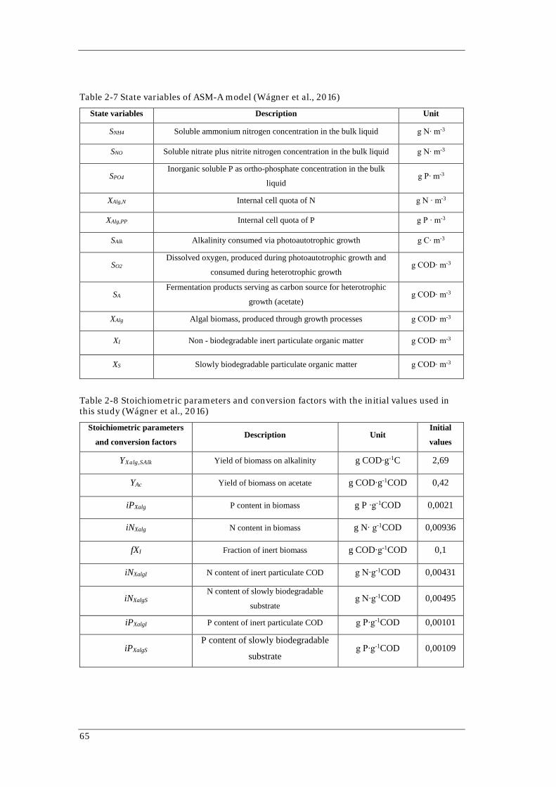
nutrient condition proposed by Geider & La Roche (2002) 32 Table 2-3 Range of variation of TN and TP in municipal wastewater 33 Table 2-4 N-to-P ratios influence on microalgae metabolism from literature. 35 Table 2-5 The Gujer matrix of ASM-A model (Wágner et al., 2016) 40 Table 2-6 Process rates of the ASM-A model (Wágner et al., 2016) 41 Table 2-7 State variables of ASM-A model (Wágner et al., 2016) 42 Table 2-8 Stoichiometric parameters and conversion factors with the initial values used
in this study (Wágner et al., 2016) 42 Table 2-9 Kinetic parameters of ASM-A model with the initial values used in this study
(Wágner, 2016) 43 Table 2-10 Upper and lower bounds, that define the ranges used during the LHSS
calibration process (Wágner, 2016) 47 Table 3-1 Lundtofte influent wastewater nutrients concentration 52 Table 3-2 Desired influent nutrients concentrations 53 Table 3-3 N-to-P ratio in R2 influent 56 Table 3-4 Initial condition in 1-L Batch experiment 58 Table 3-5 Parameters chosen to be estimated in this work 62 Table 4-1 Nutrients concentration in EBPR system effluent 66 Table 4-2 TSS values in R2 and its effluent at Day 1 and Day 2 73 Table 4-3 Parameters set estimated for 17-17 Batch and parameters set from Wagner, et
al. (2016) 82 Table 4-4 Parameters distribution and correlation matrix 84 Table 4-5 Janus coefficients used to assess the impact of the parameters variability on
the model output 85 Table 4-6 Parameters set estimated for 10-17 Batch 86 Table 4-7 Parameters distribution and correlation matrix 88

X
Table 4-8 Janus coefficients used to assess the impact of the parameters variability on
the model output 89 Table 4-9 Estimated parameters sets and the average parameters set 89 Table 4-10 Janus coefficients used to compare the simulations done using the average
parameters set and the estimated ones for both 17-17 batch and 10-17 Batch
91

XI
Abbreviations
AD Anaerobic Digester
ATP Adenosine Triphosphate
CANR Completely Autotrophic Nitrogen Removal
COD Chemical Oxygen Demand
CFS Continuous Flow reactor
EBPR Enhanced Biological Phosphorus Removal
EBP2R Enhanced Biological Phosphorus Removal and Recovery
H Reactor Depth
HRT Hydraulic Retention Time
IL Inlet Light
LHSS Latin Hypercube Sampling based Simplex
LP Light Parameter
OD Optical Density
PAO Polyphosphate Accumulating Organisms
PBR Photobioreactor
PHA Polyhydroxialcanoates
RMSNE Root Mean Square Normalized Error
SBR Sequencing Batch Reactor
R1 Reactor 1 of Continuous Flow PBR Experiment (Reference)
R2 Reactor 2 of Continuous Flow PBR Experiment
sCOD Soluble Chemical Oxygen Demand
SRT Solid Retention Time
TP Total Phosphorus
TN Total Nitrogen
TSN Total Soluble Nitrogen
TSS Total Suspended Solid
WW Wastewatater
WWTP Wastewater Treatment Plant

12
BACKGROUND AND MOTIVATIONS
1.1 Resource shortages and their increasing demand
The future of human population and Earth’s capacity to support people are highly
unpredictable, since they depend on both natural constraints and human choices (Cohen,
1995). Recent previsions suggest that, although the growth rate of the world population seems
to be decreasing, the total number of living humans on Earth is expected to rise by 50% over
the course of this century, reaching 11 billion of people (Ortiz-Ospina & Roser, 2016). Even if
these predictions do not come true, improving standard of life, urbanization, industrialization
and climate change could put a constrain on global growth. This means that we will have to
find more and more resources as food, water, raw materials and energy in a world where they
seem already scarce and where our environmental impact is at the threshold. The traditional
“take, make, waste” of the linear economy approach to managing resources is no longer
sustainable; subsequently, the interest in optimized uses of natural resources and in their
recovery from waste streams is growing encouraging the shifting to a circular economy
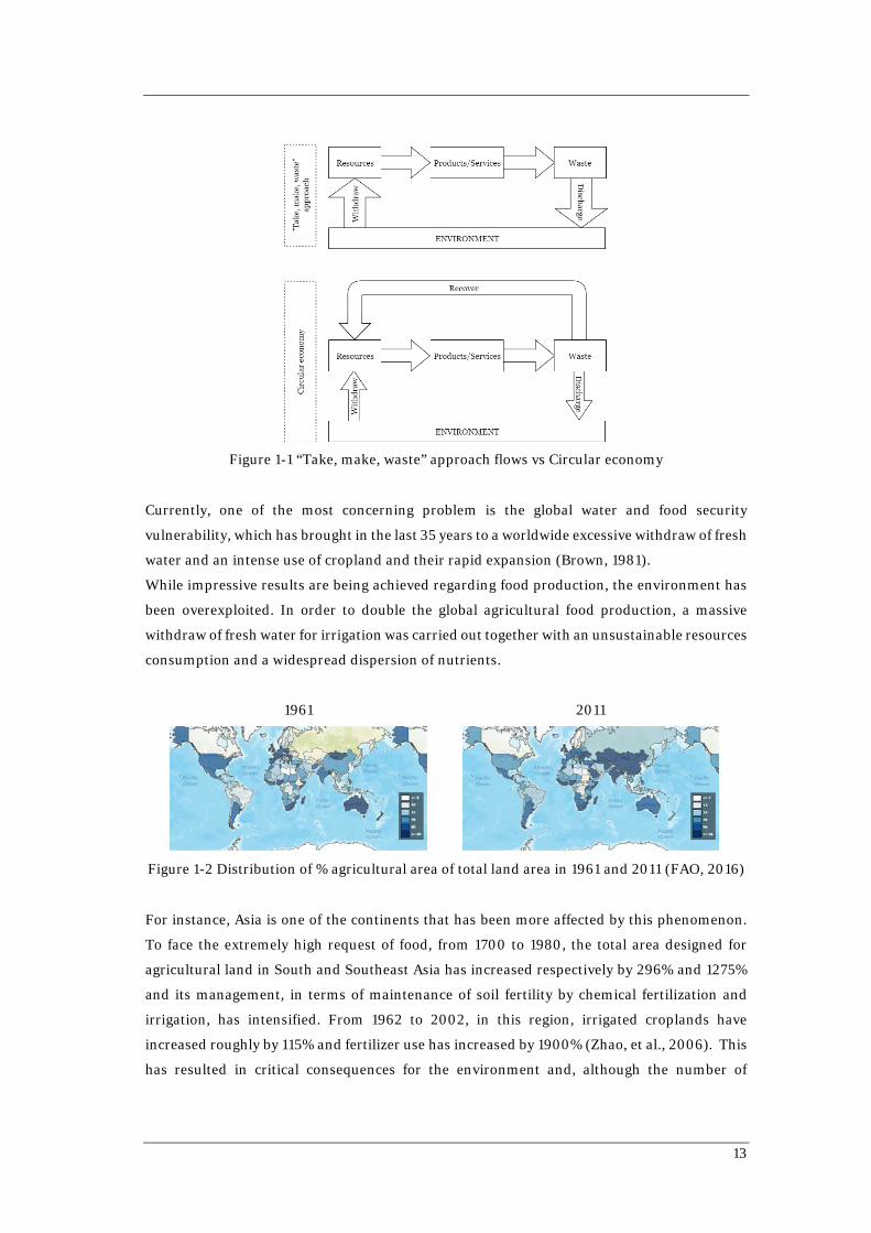
approach ( Christensen & Hauggaard-Nielsen, 2015) (Figure 1-1).
13
Figure 1-1 “Take, make, waste” approach flows vs Circular economy
Currently, one of the most concerning problem is the global water and food security
vulnerability, which has brought in the last 35 years to a worldwide excessive withdraw of fresh
water and an intense use of cropland and their rapid expansion (Brown, 1981).
While impressive results are being achieved regarding food production, the environment has
been overexploited. In order to double the global agricultural food production, a massive
withdraw of fresh water for irrigation was carried out together with an unsustainable resources
consumption and a widespread dispersion of nutrients.
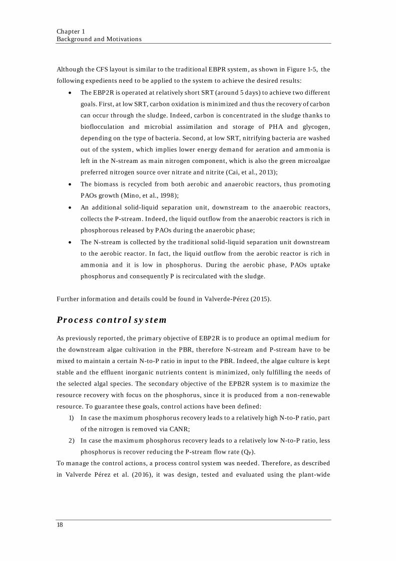
1961 2011
Figure 1-2 Distribution of % agricultural area of total land area in 1961 and 2011 (FAO, 2016)
For instance, Asia is one of the continents that has been more affected by this phenomenon.
To face the extremely high request of food, from 1700 to 1980, the total area designed for
agricultural land in South and Southeast Asia has increased respectively by 296% and 1275%
and its management, in terms of maintenance of soil fertility by chemical fertilization and
irrigation, has intensified. From 1962 to 2002, in this region, irrigated croplands have
increased roughly by 115% and fertilizer use has increased by 1900% (Zhao, et al., 2006). This
has resulted in critical consequences for the environment and, although the number of

Chapter 1 Background and Motivations
14
malnourished people in the last 20 years decreased by 30%, about 563 million of people have
to deal with the lack of food. To definitively defeat this problem, a more sustainable way has
to be found.
1.2 A new solution: Resources recovery from waste
streams – Circular Economy
One solution to the contemporary lack of resources and environment pollution seems to be the
recovery of hidden resources in waste streams.
Over the years many countries have tried to apply this idea to the solid waste. In Europe every
year, about 250 million of tons of municipal solid waste are produced and large part of these
are products with a relatively short life and a high resources and energy demanding production
(Ispra, 2014). Thus, different resource recovery system were developed. Recent studies of
ISPRA about the fate of wasted packaging report that, in 2011, 63.3% were recycled and 13,7%
were sent to incineration plants for energy recovery (Ispra, 2014). This has allowed to
considerably reduce new resources withdraw from the environment and to limit the
consumption of energy. Since good results are being achieved in the solid waste field, it is
desirable to expand this policy to other fields, such as the wastewater field.
Indeed wastewater is a resource of renewable energy, nutrients, such as nitrogen and
phosphorus, and fresh water. However, nowadays conventional wastewater treatment plants
are focused on the destruction of organic and inorganic pollutants, instead of on the recovery
of these precious resources. Moreover, most of the traditional wastewater treatment plants are
great resource consumers (CSS, 2015). Means (2004) estimated the about 4% of the public
energy use of a municipality in US is spent for WWTPs. Mo & Zhang (2012) reported that they
also require such a large amount of materials over their lifetime, that the indirect energy
embodied in those materials accounts for almost two thirds of the energy directly consumed
in the WWTPs.
Therefore, research is pushing towards the development of new technologies, which should
revolutionize the wastewater treatment.

15
Figure 1-3 Main flows in a traditional WWTP and in an innovative WWTP
Recently new technologies for resources recovery have been studied and the proposed
solutions head towards a redefinition of the conventional wastewater treatment plants.
Nonetheless, if these solutions seem efficient and able to reclaim most of the resources from
wastewater, most of them lead to such an high environmental impact, due to the intensive use
of energy and chemicals, that sometimes it switches them into a counter-productive solution
that on the whole are less sustainable than the traditional wastewater treatment plant. This
may be the limiting factor for the diffusion and the full-scale application of this new approach.
As alternative, Valverde-Pérez (2015) proposed an innovative full biochemical resource
recovery process (TRENS) that consists of an enhanced biological phosphorous removal and
recovery (EBP2R) combined with green microalgal cultivation in a photobioreactor (PBR) and
an anaerobic digester(AD). Innovative, because it is one of the few that uses only biological
treatment and that recovers efficiently water, energy and nutrients from wastewater. This
means that it could be a competitive and feasible option to meet the needs above discussed.
This thesis reconsiders Valverde-Pérez’s work and resumes it, investigating thoroughly the
PBR operation starting from the reported uncertainties and problems. In the next chapter,
TRENS system and the main related problems are described.
1.3 TRENS System
TRENS system is a completely biochemical resource recovery process, which was developed
as alternative to the current resource recovery strategies characterized by an high
environmental impact due to the high energy demand and chemicals consumption. TRENS
allows to recover large part of the hidden resources in wastewater, converting them in high
value products, such as methane for energy production and microalgae biomass combined
with water for slow leaching fertilization. Therefore, through TRENS one of the most

Chapter 1 Background and Motivations
16
problematic waste stream of the society can be converted into a solution to several current
problems. Indeed, the outputs of TRENS can benefit society by providing a clean source of
energy and by remediating the lack of nutrients and the scarcity of fresh water for crop
irrigation.
In this chapter, the description of the structure and the processes involved in TRENS is
reported, followed by the analysis of the obtained results and the observed problems.
1.3.1 Structure
TRENS consists of an enhanced biological phosphorus removal and recovery (EBP2R) and a
photobioreactor (PBR) combined with an anaerobic digester and a completely autotrophic
nitrogen removal system (CANR). In Figure 1-4 the structure of the system is represented,
focusing on the outflows.
Figure 1-4 TRENS system structure
As shown in Figure 1-4, the collected wastewater rich in carbon, nitrogen and phosphorous
enters in TRENS as input for the EBP2R system, which aim is to produce three different output
streams using bacterial based technologies. The three streams, here called C-stream, N-stream
and P-stream, are respectively rich in carbon, nitrogen and phosphorous. C-stream is directed
to the anaerobic digester, where it is used as primary element for methane production. N-
stream and P-stream are mixed properly to produce an optimum medium for algal cultivation.
In case of relatively high content of nitrogen in the medium, CANR should help to remove the
excess. While in case of low N-to-P ratio, the P-stream flow rate can be slightly decrease
without affecting the operation of the system. In PBR, microalgae grow accumulating nutrients
in their cells, thus the final output of TRENS results innocuous for the environment avoiding
soil pollution and eutrophication of groundwater, when it is used for fertigation.
The next paragraphs describe the main technologies implemented in TRENS.

17
EBP2R
EBP2R idea arises from the need to adapt the traditional wastewater treatment to the stricter
regulations on the emission of wastewater in the reservoirs and the increasing consumption
with consequent release of water and nutrients, which are limited resources.
EBP2R is based on the traditional Enhanced Biological Phosphorous Removal System (EBPR)
for phosphorous removal, which was developed in the late 50s as response to the increasing
concern on eutrophication of aquatic environment due to the release of untreated wastewater.
A complete description of the EBPR system may be found elsewhere, for instance in
Metcalf&Eddy(2014). Nevertheless, differently from EBPR, as its own name suggests, EBP2R
not only aims to remove the nutrients from the incoming wastewater, but it is also proposed
to recover these nutrients in order to reuse them in other applications.
As mentioned in the previous paragraph, EBP2R has the objective to produce three different
output streams, each one rich in a different nutrient (carbon, nitrogen or phosphorous) to
guarantee constant inputs to the following technologies in TRENS.
Layouts and processes
Two different layouts for EBP2R were proposed and studied: a continuous flow system,
referred as CFS, and a sequencing batch reactor. Anyhow, the objectives of this work are based
on the issues related to the first layout, therefore only the CFS is considered and described in
this paragraph.
Figure 1-5 EBP2R in the Continuous Flow System layout (CFS) (Valverde Perez, 2015)
Chapter 1 Background and Motivations
18
Although the CFS layout is similar to the traditional EBPR system, as shown in Figure 1-5, the
following expedients need to be applied to the system to achieve the desired results:
• The EBP2R is operated at relatively short SRT (around 5 days) to achieve two different
goals. First, at low SRT, carbon oxidation is minimized and thus the recovery of carbon
can occur through the sludge. Indeed, carbon is concentrated in the sludge thanks to
bioflocculation and microbial assimilation and storage of PHA and glycogen,
depending on the type of bacteria. Second, at low SRT, nitrifying bacteria are washed
out of the system, which implies lower energy demand for aeration and ammonia is
left in the N-stream as main nitrogen component, which is also the green microalgae
preferred nitrogen source over nitrate and nitrite (Cai, et al., 2013);
• The biomass is recycled from both aerobic and anaerobic reactors, thus promoting
PAOs growth (Mino, et al., 1998);
• An additional solid-liquid separation unit, downstream to the anaerobic reactors,
collects the P-stream. Indeed, the liquid outflow from the anaerobic reactors is rich in
phosphorous released by PAOs during the anaerobic phase;
• The N-stream is collected by the traditional solid-liquid separation unit downstream
to the aerobic reactor. In fact, the liquid outflow from the aerobic reactor is rich in
ammonia and it is low in phosphorus. During the aerobic phase, PAOs uptake
phosphorus and consequently P is recirculated with the sludge.
Further information and details could be found in Valverde-Pérez (2015).
Process control system
As previously reported, the primary objective of EBP2R is to produce an optimal medium for
the downstream algae cultivation in the PBR, therefore N-stream and P-stream have to be
mixed to maintain a certain N-to-P ratio in input to the PBR. Indeed, the algae culture is kept
stable and the effluent inorganic nutrients content is minimized, only fulfilling the needs of
the selected algal species. The secondary objective of the EPB2R system is to maximize the
resource recovery with focus on the phosphorus, since it is produced from a non-renewable
resource. To guarantee these goals, control actions have been defined:
1) In case the maximum phosphorus recovery leads to a relatively high N-to-P ratio, part
of the nitrogen is removed via CANR;
2) In case the maximum phosphorus recovery leads to a relatively low N-to-P ratio, less
phosphorus is recover reducing the P-stream flow rate (QP).
To manage the control actions, a process control system was needed. Therefore, as described
in Valverde Pérez et al. (2016), it was design, tested and evaluated using the plant-wide
19
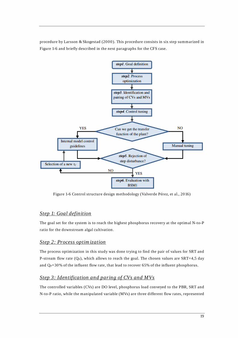
procedure by Larsson & Skogestad (2000). This procedure consists in six step summarized in
Figure 1-6 and briefly described in the next paragraphs for the CFS case.
Figure 1-6 Control structure design methodology (Valverde Pérez, et al., 2016)
Step 1: Goal definition
The goal set for the system is to reach the highest phosphorus recovery at the optimal N-to-P
ratio for the downstream algal cultivation.
Step 2: Process optimization
The process optimization in this study was done trying to find the pair of values for SRT and
P-stream flow rate (QP), which allows to reach the goal. The chosen values are SRT=4,5 day
and QP=30% of the influent flow rate, that lead to recover 65% of the influent phosphorus.
Step 3: Identification and paring of CVs and MVs
The controlled variables (CVs) are DO level, phosphorus load conveyed to the PBR, SRT and
N-to-P ratio, while the manipulated variable (MVs) are three different flow rates, represented
Chapter 1 Background and Motivations
20
in Figure 1-5 as valves: P-stream flow rate (QP), wastage flow rate (QW) and N-stream flow rate
(QN). From the pairing of these variables it results that the SRT is controlled by QW, the
phosphorus load conveyed to the PBR is controlled by QP and the N-to-P ratio is controlled by
the QN. Indeed, regarding the DO level in the aerobic tank, air supply is used to keep the oxygen
level at 1,5 mg/l.
Step 4: Controller tuning
Controller tuning refers to the selection of tuning parameters to ensure the best response of
the controller. In this case, the controllers were modeled as Proportional Integral (PI)
controllers and they were either tuned following the internal model control (IMC) rules or
manual tuned, when the transfer function cannot be obtained (Sebog, et al., 2004; Skogestad,
2003).
Step 5: Rejection of step disturbances?
The system was subjected to step disturbances in the influent quality to assess the ability of
the control system to keep the system stable. In case of failure, the procedure re-started from
Step 4. During this phase, only one factor at time was changed and the step was introduced in
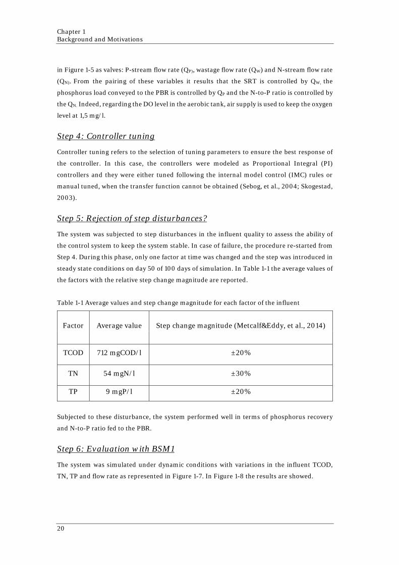
steady state conditions on day 50 of 100 days of simulation. In Table 1-1 the average values of
the factors with the relative step change magnitude are reported.
Table 1-1 Average values and step change magnitude for each factor of the influent
Factor Average value Step change magnitude (Metcalf&Eddy, et al., 2014)
TCOD 712 mgCOD/l ±20%
TN 54 mgN/l ±30%
TP 9 mgP/l ±20%
Subjected to these disturbance, the system performed well in terms of phosphorus recovery
and N-to-P ratio fed to the PBR.
Step 6: Evaluation with BSM1
The system was simulated under dynamic conditions with variations in the influent TCOD,
TN, TP and flow rate as represented in Figure 1-7. In Figure 1-8 the results are showed.

21
Figure 1-7 Influent to the EBP2R (Valverde Pérez, et al., 2016)
Figure 1-8 Phosphorus load and N-to-P ratio in input to the PBR under dynamic condition in
the CFS case (Valverde-Pérez, 2015).
The results show that if the control system is mainly able to smooth variation of P-load, it is
not able to keep the N-to-P ratio at a setpoint level (17 molN/molP). Although the peaks of N-
to-P ratio, shown by the open loop system, are toned down, the N-to-P ratio regularly falls
under the optimum value.
- Without process system control - With process system control

Chapter 1 Background and Motivations
22
PBR
The optimal cultivation medium produced in the previous step is sent to the PBR, where the
selected microalgae culture is spurred to grow using the incoming nutrients together with light
and CO2 that have to be supplied to the system. Carbon dioxide may be delivered through a
gaseous flow rich in CO2 originated from the biogas combustion in the cogeneration units, that
potentially could follow the anaerobic digester (Napan, et al., 2015). At the same time, this flow
can also guarantee a proper mixing in the reactor.
In these optimal conditions, the growth medium is optimized and nutrients are encapsulated
inside algae biomass, thus the effluent from PBR is composed by algal biomass suspended in
the treated water with a low inorganic nutrients load. To avoid harvesting costs, which are one
of the main problem related to the latest microalgae based technologies (Liu & Vyverman,
2015), the effluent can be directly applied to the land for crops fertigation (Wilkie & Mulbry,
2002). Indeed, microalgae had shown good properties as natural fertilizer (Mulbry, et al.,
2005) and the risk of soil pollution and ground water eutrophication is minimized thanks to
the low concentration of pollutants in the treated water. Through drip irrigation, the effluent
can reach directly the roots area in the cropland. When the algae biomass in suspension in the
effluent reaches the ground, it settles and, according to Mulbry et al. (2005), it starts to release
nutrients in an available form for crops uptake. The water instead accumulates in the soil until
the field capacity is reached. Afterwards, it starts to leach towards the groundwater. If it
reaches the aquifer, it does not represent a problem, because, as it was explained previously,
the concentration of pollutants in the water is minimal, thus the risk of contamination of the
ground water is minimized. This is a great advantage over using raw wastewater or treated
wastewater from a traditional wastewater treatment plant as irrigation water (Figure 1-9).
Indeed, they can potentially compromise the groundwater quality and therefore its withdraw
for other purposes.
Figure 1-9 TRENS effluent application in fertigation

23
Anaerobic digester
As previously specified, the third stream produced by EBP2R is rich in carbon and thus organic
matter, which is the main component required in input at the anaerobic digester for methane
production. The anaerobic digestion of waste activated sludge is a technology relatively well
established, which has been studied and developed to give a solution to the costly disposal of
this waste. Indeed, not only it has the abilities to destroy most of the pathogens present in the
sludge and to limit the odor problems related to the residual putrescible matter, but it also
transforms the residual organic matter into biogas with an average content of methane about
55%vol-75%vol (De Mes, et al., 2003). This means that from the C- stream a further recovery
of resources is possible through the production of energy from biogas (Apples et al., 2008).
More information about anaerobic digestion may be found elsewhere (Apples, et al., 2008)
(Carballa, et al., 2015).
CANR
In case of relatively high content of nitrogen in the wastewater, which could lead to an N-to-P
ratio higher than the set one, to meet the request of the PBR the process control system send
part of the N-stream to the CANR. CANR is a new biological nitrogen removal process based
on a partial nitrification and anoxic oxidation of ammonia. Therefore, it almost completely
converts the ammonia presents in the N-stream into dinitrogen gas. The process works
properly with the N-stream from EBP2R, since it can treat wastewater that contains low
amounts of organic material. However, this process has not been fully tested yet and it is still
in the experimental phase. More information about CANR may be found elsewhere (Khin &
Annachhatre, 2004; Mutlu, et al., 2013).
1.3.2 Results: achievements and limitations
Valverde-Pérez (2015) has demonstrated the efficiency of EBP2R in separation and recovery
of phosphorus and nitrogen from municipal wastewater via model-based studies. The
continuous EBP2R allows to recover 65% maximum of the influent phosphorus through P-
stream. Nevertheless, phosphorus recovery was found to be limited by EBP2R SRT and nitrate
presence in the anaerobic reactors. Indeed, anoxic enviroments can appear promoting
denitrification over phosphorus release. Moreover, in the continuous EBP2R, PAOs growth
can be limited by phosphorus availability in the aerobic reactor.
The control system has been tested using dynamic input disturbance scenarios and it results
to be able to keep constant the P load in input to the PBR, but it fails to limit the variation of
the N-to-P ratio when the influent nitrogen to the EBP2R becomes limiting. Even if the
variations from the optimal N-to-P ratio are not severe, some aspects need to be studied. For
Chapter 1 Background and Motivations
24
instance, the effects on the PBR effluent quality and the green microalgae culture stability.
Indeed, according to Beuckles, et al. (2015), N-to-P ratio seems to drive competition between
algal species in algae consortia. Moreover, it could weaken the culture facilitating
contaminations.
Another aspect underlined by Valverde-Pérez (2015) is the culture history effect on maximum
nitrate uptake rate. Indeed, during laboratory experiment, where the design allowed to
distinguish between the impact of culture history and the impact of substrate availability, the
maximum nitrate uptake results higher after a period of supplied nitrogen limitation, which
could occur when the supply N-to-P ratio to the PBR drops from circa 17molN/molP to circa
10molN/molP.
TRENS system’s strengths and weaknesses have been studied by a life cycle assessment (Fang,
et al., 2015). Environmental benefits of nutrients recycling through fertigation were
highlighted, even if they may be compromised by the discharge of heavy metal on land.
Micropollutants are also an important aspect, since the low SRT in the EBP2R doesn’t facilitate
their removal (Polesel, et al., 2015) and legislations are moving towards the recognition of
those substances as harmful to the environment (Plosz & Polesel, 2015).
1.4 Thesis objectives
The aim of this thesis is to investigate the consequences in the PBR of the variation of the N-
to-P ratio in the supplied influent.
In particular, this thesis is focused on:
1. The assessment of the green microalgae culture stability in terms of composition and
contamination;
2. The evaluation of the influence of the green microalgae culture history on the uptake
and storage of nitrogen and phosphorus, studying the kinetics of the processes
involved in the PBR;
3. The development of a new images analysis method to quantify the microbial
community.

25
STATE OF ART
The term algae was first introduced by Linnaeus in 1753 to refer to a group of plants, which
are known since ancient civilization. It refers to a wide group of unicellular and multicellular
organisms present worldwide in different habitats, that can grow photoautotrophically,
heterotrophically and even mixotrophically (Van Wagenen, et al., 2015), depending on the
different environmental conditions.
Phototrophic microalgae are unicellular microorganisms capable of efficiently converting
CO2, sunlight and some basic nutrients into high valuable and energy-rich products. They
cover indispensable roles: not only they are the base for aquatic food chain, but they are
responsible for the production of more than 75% of oxygen consumed by animals and humans
(Posten & Walter, 2012). Although this may seem implausible, given the small size of the
microalgae, it became possible due to microalgae abundance and diversification. Indeed,
thanks to the singular evolution, that has affected microalgae history, their biodiversity
became remarkable and innumerable species of microalgae were found all over the world.
Even if the number of known species is already vast, around 35.000, it was estimated that
undiscovered species may exceed known species by a factor of four to eight (Norton, et al.,
1996). Since microalgae evolutionary history is uncertain and their characteristics are various,
a consistent classification for microalgae, as well as a deep understanding of their biology, is
still in progress and it needs improvement.
In the great biodiversity of this group, main groups of microalgae were established, for
instance the so-called green microalgae, which is the group of particular relevance for this
work. This group was studied and investigated due to their potential applications in several
fields and guidelines for their cultivation have been identified.

Chapter 2 State of art
26
In the first part of the chapter, the processes involved in green microalgae cultivation are
described and analyzed with focus on the main influent factors on green microalgae growth
and nutrients uptake and storage. A deepening on green microalgae cultivation in wastewater
and the relative issues is also reported. Finally, a literature review about the studies conducted
to understand the effects of nutrients variation in the medium on microalgae growth is
reported.
In the second part of the chapter, a brief literature review on the modeling applied to
microalgae is presented, followed by the description of the ASM-A model and its relative
parameters estimation procedure, which were used in this work.
2.1 Green microalgae cultivation
As previously mentioned, algae are present worldwide and they have adapted to live in several
environments under different conditions. Nevertheless, some factors are required to ensure
an optimal growth. For green microalgae, the most relevant factors are light and nutrients,
which are carbon, nitrogen and phosphorus. According to the Liebig’s law of the minimum,
the deficiency of one of those elements could deeply compromise algal growth. As reported in
Spaargaren (1996), each essential element has to be present in adequate quantity, in
appropriate ratio and in the bioavailable chemical form in the cultivation medium, so that
microalgae growth will not be limited.
It is important to underline that the chemical form of nutrients in the cultivation medium, in
particular of carbon, and the need of light vary depending on the type of growth used by green
microalgae. Indeed, as mentioned before, algae are able to grow in three different ways:
photoautotrophically, heterotrophically and mixotrophically.
Photoautotrophic green microalgae metabolism is driven by photosynthesis. Through
photosynthesis, green microalgae are able to use light as energy source to assimilate water,
inorganic carbon and nutrients and to produce new biomass compounds and oxygen (Figure
2-1).
Figure 2-1 Green microalgae photosynthesis

27
Heterotrophic green microalgae, instead, are able to grow in complete darkness, if oxygen and
an organic carbon source are supplied.
Mixotrophic green microalgae represent a particular case, since in presence of light and
organic carbon, they are able to simultaneously photosynthesize while assimilating and
metabolizing organic carbon. (Van Wagenen, et al., 2015; Smith, et al., 2015).
Table 2-1 Type of carbon source and light presence for each type of growth
Type of growth Type of carbon source Presence of light
Photoautotrophic Inorganic yes
Heterotrophic Organic no
Mixotrophic Inorganic + Organic yes
Light
Light is the energy source used by green microalgae during the photosynthesis. Therefore, light
is one of the most important factors in green microalgal cultivation and it must be considered
during the optimization of the PBR performance (Grognard, et al., 2014). In particular, to
maximize algal productivity, attention must be payed to the light attenuation along the PBR
due to self-shading.
Even if the impact of light depends on the specie of the cultivated green microalgae, some
general aspects are recognizable. Generally, light type and intensity greatly affect both algal
growth and biomass composition. Indeed algal growth rate has the tendency to increase with
light intensity until a maximum is reached. This maximum coincides with the intensity where
green microalgae cannot utilize more photons for photosynthesis and all the extra energy is
converted to heat. Instead, if the light intensity is too high algal growth rate may decrease due
to light inhibition (Sorokin & Krauss, 1958). Regarding algal composition, different effects
were found. For instance, Seyfabadi, et al. (2011) reported that at high light intensity green
microalgae have the tendency to produce more pigments for light protection. Instead, at low
light intensity, Van Wagenen, et al.( 2012) has shown that the relative abundance of
unsaturated fatty acids increases.
Carbon
Up to 65% of dry weight of green microalgae is made of carbon, indeed, it contributes to all
organic compounds in the cells (Markou, et al., 2014).
Green microalgae are able to assimilate both inorganic and organic carbon, depending on the
type of growth they have developed to live in a particular environment.
Chapter 2 State of art
28
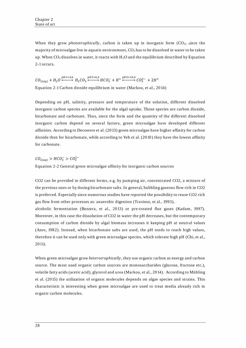
When they grow phototrophically, carbon is taken up in inorganic form (CO2). Since the
majority of microalgae live in aquatic environment, CO2 has to be dissolved in water to be taken
up. When CO2 dissolves in water, it reacts with H2O and the equilibrium described by Equation
2-1 occurs.
𝐶𝐶𝐶𝐶2(𝑎𝑎𝑎𝑎) + 𝐻𝐻2𝐶𝐶𝑝𝑝𝑝𝑝1≈3,6�⎯⎯⎯⎯� 𝐻𝐻2𝐶𝐶𝐶𝐶3
𝑝𝑝𝑝𝑝2≈6,3�⎯⎯⎯⎯� 𝐻𝐻𝐶𝐶𝐶𝐶3− + 𝐻𝐻+ 𝑝𝑝𝑝𝑝3≈10,3
�⎯⎯⎯⎯⎯� 𝐶𝐶𝐶𝐶32− + 2𝐻𝐻+
Equation 2-1 Carbon dioxide equilibrium in water (Markou, et al., 2014)
Depending on pH, salinity, pressure and temperature of the solution, different dissolved
inorganic carbon species are available for the algal uptake. Those species are carbon dioxide,
bicarbonate and carbonate. Thus, since the form and the quantity of the different dissolved
inorganic carbon depend on several factors, green microalgae have developed different
affinities. According to Decostere et al. (2013) green microalgae have higher affinity for carbon
dioxide then for bicarbonate, while according to Yeh et al. (2010) they have the lowest affinity
for carbonate.
𝐶𝐶𝐶𝐶2(𝑎𝑎𝑎𝑎) > 𝐻𝐻𝐶𝐶𝐶𝐶3− > 𝐶𝐶𝐶𝐶32−
Equation 2-2 General green microalgae affinity for inorganic carbon sources
CO2 can be provided in different forms, e.g. by pumping air, concentrated CO2, a mixture of
the previous ones or by dosing bicarbonate salts. In general, bubbling gaseous flow rich in CO2
is preferred. Especially since numerous studies have reported the possibility to reuse CO2 rich
gas flow from other processes as: anaerobic digestion (Travieso, et al., 1993),
alcoholic fermentation (Bezzera, et al., 2013) or pre-treated flue gases (Kadam, 1997).
Moreover, in this case the dissolution of CO2 in water the pH decreases, but the contemporary
consumption of carbon dioxide by algal biomass increases it keeping pH at neutral values
(Azov, 1982). Instead, when bicarbonate salts are used, the pH tends to reach high values,
therefore it can be used only with green microalgae species, which tolerate high pH (Chi, et al.,
2011).
When green microalgae grow heterotrophically, they use organic carbon as energy and carbon
source. The most used organic carbon sources are monosaccharides (glucose, fructose etc.),
volatile fatty acids (acetic acid), glycerol and urea (Markou, et al., 2014). According to Mühling
et al. (2015) the utilization of organic molecules depends on algae species and strains. This
characteristic is interesting when green microalgae are used to treat media already rich in
organic carbon molecules.
29
When green microalgae grow mixotrophically, they consume inorganic and organic carbon
sources (Van Wagenen, et al., 2015). Therefore, what has been reported for photoautotrophic
and heterotrophic growth is applicable to this case.
Nitrogen
From 1% to 14% of dry weight of green microalgae is made of nitrogen. Indeed, it is used to
build many essential compounds, such as nucleic acids, amino acids and pigments (Markou,
et al., 2014).
Green microalgae can use both inorganic and organic nitrogen form. The most commonly
reported forms are, in affinity order: ammonia, nitrate, nitrite and urea (Valverde-Pérez, et al.,
2015).
Ammonia/ammonium is the preferred nitrogen source, because its uptake and assimilation is
less energy demanding than the other forms of nitrogen. (Pérez-Garcia, et al., 2011) Moreover,
it can be directly converted to biomolecules (Cai, et al., 2013). Nevertheless, free ammonia has
detrimental effects on green microalgae at relative low concentration (Azov & Goldman, 1982).
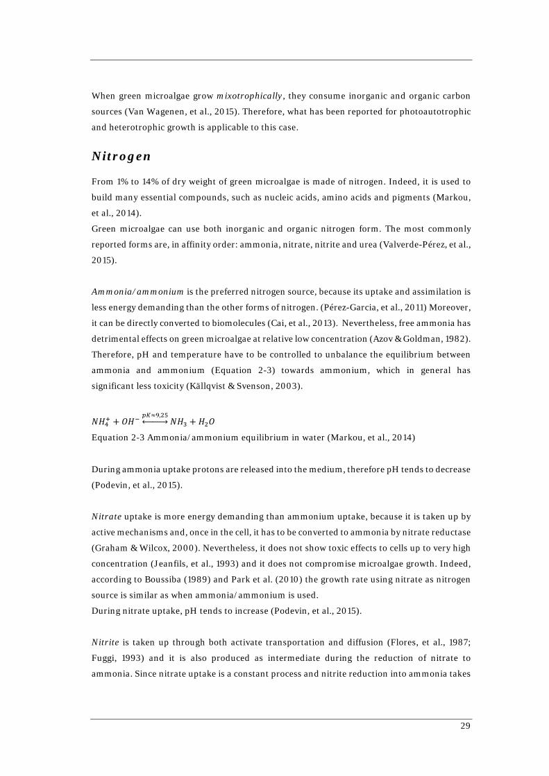
Therefore, pH and temperature have to be controlled to unbalance the equilibrium between
ammonia and ammonium (Equation 2-3) towards ammonium, which in general has
significant less toxicity (Källqvist & Svenson, 2003).
𝑁𝑁𝐻𝐻4+ + 𝐶𝐶𝐻𝐻− 𝑝𝑝𝑝𝑝≈9,25�⎯⎯⎯⎯� 𝑁𝑁𝐻𝐻3 + 𝐻𝐻2𝐶𝐶
Equation 2-3 Ammonia/ammonium equilibrium in water (Markou, et al., 2014)
During ammonia uptake protons are released into the medium, therefore pH tends to decrease
(Podevin, et al., 2015).
Nitrate uptake is more energy demanding than ammonium uptake, because it is taken up by
active mechanisms and, once in the cell, it has to be converted to ammonia by nitrate reductase
(Graham & Wilcox, 2000). Nevertheless, it does not show toxic effects to cells up to very high
concentration (Jeanfils, et al., 1993) and it does not compromise microalgae growth. Indeed,
according to Boussiba (1989) and Park et al. (2010) the growth rate using nitrate as nitrogen
source is similar as when ammonia/ammonium is used.
During nitrate uptake, pH tends to increase (Podevin, et al., 2015).
Nitrite is taken up through both activate transportation and diffusion (Flores, et al., 1987;
Fuggi, 1993) and it is also produced as intermediate during the reduction of nitrate to
ammonia. Since nitrate uptake is a constant process and nitrite reduction into ammonia takes

Chapter 2 State of art
30
place only when light is available, under light limitation, nitrite can accumulate in the cells
(Brussaard, et al., 1998) and thus, it may be released in the medium due to its toxic effect at
high concentration (Malerba, et al., 2012). Moreover, if nitrate concentration is too high,
nitrite can accumulate in the cells even in non-light limitation condition, inhibiting microalgae
growth (Jeanfils, et al., 1993).
Urea and some amino acids are taken up actively and are metabolized in the cells (Pérez-
Garcia, et al., 2011; Flores & Herrero, 2005). Some green microalgae seem not only to be able
to use organic nitrogen, but, when they use these molecules, their growth rate are similar or
higher than when they use other inorganic forms of nitrogen. However, the possibility to use
organic nitrogen compounds as nitrogen resource is species dependent (Flores & Herrero,
2005).
It has to be noted that, when different nitrogen sources are simultaneously present in the
medium, green microalgae firstly uptake the more affine depleting it, then they uptake the
others (Boussiba & Gibson, 1991).
Phosphorus
From 0,05% to 3,3% of dry weight of green microalgae is made of phosphorus. Indeed, it is
used to build several essential compounds, such nucleic acids, membrane phospholipids and
ATP (Markou, et al., 2014).
Phosphorus is taken up actively by green microalgae when it is in orthophosphate form.
Organic forms of phosphorus can also be used once they are mineralized extracellularly by
phosphatase enzymes (Dyhrman & Ruttenberg, 2006).
Nutrients limitation
In natural environments algae may be exposed to nutrients limitation, therefore they had
developed different strategies to manage these non-optimal conditions enabling adaptation
across a wide range of environments (Loladze & Elser, 2011)
They can either encapsulate excess quantities of nutrients in period of nutrients abundance
(Eixler, et al., 2006) or grow with lower quantity of nutrients, changing their internal
composition.
In fact, green microalgae had shown the so-called luxury uptake of nutrients, which is the
capacity to accumulate intracellular phosphorus and nitrogen reserves (Powell, et al., 2009;
Pueschel & Korb, 2001). This storage can be used by algae under starving conditions. Until it
31
is depleted, algal activity it is not affected by the environmental conditions as well as growth
rate and the algal biomass composition (Beuckles, et al., 2015; Ruitz-Martinez, et al., 2014).
When the internal reserves of nutrients are not available, green microalgae adapt their
biomass in response. Indeed, the algal biomass is generally mainly made of biochemical
compounds rich in N and P, but, when N and P became limited, algae are able to change their
internal composition (Beuckels et al, 2015; Choi & Lee, 2015), increasing the internal
percentage of carbon-rich compounds, as carbohydrates and lipids.
N-to-P ratio
In 1934 Alfred Redfield first proposed the theory that marine phytoplankton, i.e. unicellular
microalgae and cyanobacteria, has relatively constrained elemental ratios. It means that there
is a relationship between organisms’ growth and internal composition and the ratio of the
elements in the surrounding environment. In particular, nitrogen and phosphorus have been
recognized to be highly influential factors. Therefore, their singular and relative availability in
the growth medium is crucial. In 1958 Redfield concluded that the optimal ratio for marine
phytoplankton for those nutrients was 16 molN/molP, which coincides with the average N-to-
P ratio found in the studied organisms. However, as mentioned before, the internal algal N-
to-P ratio may vary in relation to the surrounding conditions. Several studies have been carried
out to investigate the effective N-to-P ratio in microalgae composition, its variability and the
critical medium N-to-P ratio, that determines changing in microalgae behavior.
Variability of internal N-to-P ratio and critical medium N-to-P ratio
(Geider & La Roche, 2002)
In 2002, Geider and La Roche had tried to determine the range of the variability of the N-to-
P ratio for different species of algae and cyanobacteria using a compilation of data on the
elemental composition of marine phytoplankton. The traditional Redfield’s N-to-P ratio is
used as criterion to distinguish N-limitation from P-limitation assuming that a N-to-P ratio
lower than 16 molN/molP corresponds to a nitrogen limitation and a N-to-P ratio higher than
16 molN/molP corresponds to a phosphorus limitation. Instead, in their study, it is shown that
the internal N-to-P ratio can vary within different ranges in relation to the condition where
organisms are growing. In nutrient-limited cells the N-to-P ratio is very plastic and can vary
from < 5 molN/molP, when nitrogen is greatly limited, to >100 molN/molP, when nitrogen is
present in large excess. The cellular N-to-P ratio is more constrained when the concentration
of inorganic nutrients in solution is several-fold greater than the half saturation constants for
nutrients assimilation (from 0,001 to 15 gN/m3 for NH4+ and NO3-; from 0,001 to 5 gP/m3 for
PO43-). In fact, it ranges from 5molN/molP to 19 molN/molP.

Chapter 2 State of art
32
Table 2-2 Ranges of internal N-to-P ratio in nutrients limited condition and optimal nutrient condition proposed by Geider & La Roche (2002)
Internal N-to-P ratio
Lower boundary Upper boundary
[molN/molP] [molN/molP]
Nutrients limited condition <5 >100
Optimal nutrients condition 5 19
The critical N-to-P ratio, that marks the transition between N-limitation and P-limitation, was
found to lie in a range between 15 molN/molP and 30 molN/molP.
2.2 Microalgae cultivation in wastewater
Over 50 years ago in the U.S., Oswald & Gotaas (1957) had proposed the biological treatment
of wastewater with algae to remove nutrients such as nitrogen and phosphorus. This idea has
since been intensively tested all over the world, together with the study of the potential
utilizations the algal biomass (Abdel-Raouf, et al., 2012).
The application of microalgae in the wastewater treatment has several advantages, i.e. the
removal of coliform bacteria (Moawad, 1968; Sebastian & Nair, 1984), the reduction of both
chemical and biochemical oxygen demand (Colak & Kaya, 1988), the removal of nitrogen and
phosphorus (Talbot & De la Noue, 1993) and also the removal of heavy metals (Rai, et al.,
1981). This may help to avoid secondary pollution in reservoirs due to the residual nutrients,
which can lead to eutrophication, uncontrolled spread of certain aquatic macrophytes, oxygen
depletion, loss of key species and degradation of fresh water ecosystems (Wang, et al., 2010;
Doria, et al., 2012). Moreover, through photosynthesis microalgae convert solar energy into
useful and valuable biomass requiring less land than a traditional crop (Liu & Vyverman,
2015).
Microalgae perform well, in terms of nutrients removal and biomass production, treating
different wastewater: municipal wastewater (Li, et al., 2011; Shelef, et al., 1980; Chi, et al.,
2011), livestock wastes (Lincon & Hill, 1980), agro-industrial wastes (Mulbry, et al., 2009;
Mulbry, et al., 2008) and industrial wastes (Markou & Georgakakis, 2011).
Microalgae have been proposed to be applicable in the secondary (Tam & Wong, 1989), tertiary
(Lavoie & De la Noue, 1985; Martin, et al., 1985a; Evonne & Tang, 1997) and higher treatments
(Oswald, 1988b). In general, their application in tertiary treatment and higher treatment
seems to be less cost and energy demanding than other technologies (Abdel-Raouf, et al.,
2012).

33
Hence, microalgae cultivation seems to be a good alternative as a biological treatment method
for wastewater ( Cai , et al., 2013).
2.2.1 Nutrients variation in wastewater
Wastewater has been shown to be a suitable medium for algal growth, because it can provide
most of the necessary nutrients (Renuka, et al., 2013).
As mentioned before, algae can grow in wastewater from different origins. Nevertheless, its
composition vary with sources and many other variables ( Cai , et al., 2013).
For instance, municipal wastewater is mostly composed by discharged water from residential
areas, commercial and institutional facilities and industries and potentially stormwater.
Therefore, its quantity and quality undergo substantial variations in time (in short term and
in long term) and in space (Henze & Comeau, 2008).
This variability can represent an obstacle to the application of microalgae in wastewater
treatment. Indeed, nutrient components greatly affect the microalgae growth rate, the uptake
and storage of nutrients and the biomass composition. In particular, the key elements for
microalgae cultivation are nitrogen and phosphorus. As reported Table 2-3, the ranges of
variation of these components have been found to be very wide (Henze & Comeau, 2008; Cai,
et al., 2013; Muttamara, 1996; Carey & Migliaccio, 2009) and consequently the N-to-P ratio.
Indeed, it can vary from 1,33 molN/molP to 55 molN/molP.
Table 2-3 Range of variation of TN and TP in municipal wastewater
Range
TN [mgN/l] 15-100
TP [mgP/l] 4-25
Since according to Geider & La Roche (2002), the critical N-to-P ratio in the growth medium
can vary between 15 molN/molP and 30 molN/molP in order to guarantee an optimal algal
cultivation, the variability of the raw municipal wastewater here reported is too large and it
may compromise the process.
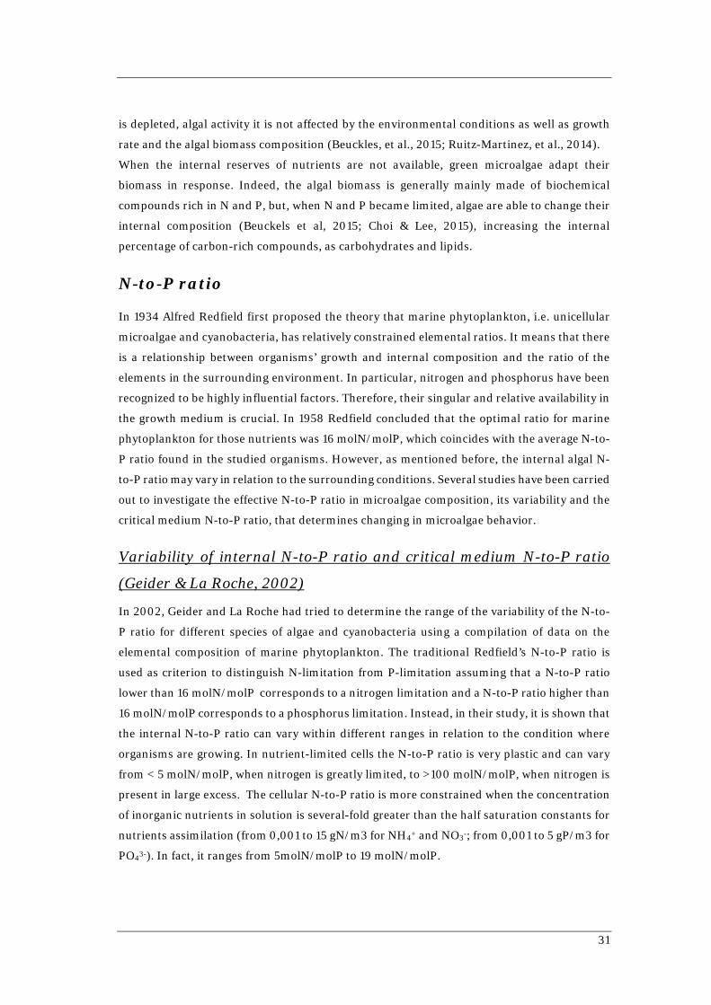
Effects of medium N-to-P ratio
To understand the effects of the medium N-to-P ratio and its variation on the culture, a
deepened review of studies reported in literature was carried out. Most of the studies, found
in literature about N-to-P ratio implications, were conducted in batch reactors and only few
report experiments in other reactor configurations(semi-continuous reactor). Therefore, it has
been decided to study articles where batch reactor experiments were performed. In some

Chapter 2 State of art
34
studies, the N-to-P ratio was controlled changing only one nutrient (either P or N), in others
changing both with the idea to test the limitation of one nutrient by time. In the selected
articles, it was possible to find a relation between the N-to-P ratio in the medium and the N-
and P-uptake and growth rate. In Table 2-4 the summary of these studies is reported.
35
Table 2-4 N-to-P ratios influence on microalgae metabolism from literature.
S= Synthetic Medium; WW = Wastewater; W=Freshwater.
Article Algae specie Medium N-to-P ratio
[molN/molP]
N range
[mgN/l] P range
[mgP/l] Results on N- and
P- uptake
Results on growth
rate
Liu &
Vyverman
(2015)
Cladophora sp.
Klebsormidium sp.
Pseudanabaena sp.
S 1-20 5 0,5 - 10
P-Uptake directly ∝
N-to-P ratio;
N-Uptake
independent of N-to-
P ratio
N-to-P ratio affects the
growth rate, but the
effect is species-specific
Whitton, et
al. (2016)
Chlorella vulgaris
Scenedesmus
obliquus
WW 1.1 – 22.1 6,77 - 14 31 – 1,5
P-uptake directly ∝
N-to-P ratio;
N-uptake inversely ∝
N-to-P ratio
N-to-P ratio affects the
growth rate
(no more info)
Choi & Lee
(2015) Chlorella vulgaris WW
1-80
(changing both
P and N)
- -
P-Uptake directly ∝
N-to-P ratio;
N-Uptake
independent of N-to-
P ratio
Growth rate is highly
dependent on the N-to-
P ratio. It increases
until N-to-P=10 then
gradually decreases
reaching a minimum at
N-to-P=30
Seung-
Hoon, et al.
(2013)
Consortium WW 120 and 31 7,04 0,13 and
0,5
N- and P-uptake
higher at 31 N-to-P
ratio
N-to-P ratio affects the
growth rate
(no more info)

Chapter 2 State of art
36
Arbib, et al.
(2013)
Scenedesmus
obliquus WW 1 -35
22,77
–
92,77 5,69 - 40
P-uptake directly ∝
N-to-P ratio; N-
Uptake independent
of N-to-P ratio
No significant influence
of N-to-P ratio on
growth rate except a
slight reduction for N-
to-P ratio = 35
Suttle &
Harrison
(1988)
Consortium W +S 5 -45 35 - 10 2 – 0,5
P-uptake directly ∝
N-to-P ratio;
N-uptake inversely ∝
N-to-P ratio
-
Rhee (1978) Scenedesmus sp. S 5-80
0,21
–
3,36 0,093
N-uptake inversely ∝
N-to-P ratio;
Growth rate increases
linearly with N-to-P
until 30, then levels off -
> N limitation before 30
Li, et al.
(2010) Scenedesmus sp. S 2-100 2,5 - 25 0,1 - 2
P-uptake
independent of N-to-
P ratio;
N-uptake inversely ∝
N-to-P ratio
Growth rate is
independent of N-to-P,
until N or P becomes
limiting

37
These studies generally show a dependency of microalgae metabolism on nutrients availability
and the N-to-P ratio in the medium. For instance, the growth rate seems to be affected by the
N-to-P ratio and it is sensitive to the depletion of nutrients.
Nevertheless, it was hard to find other trends among the studies. The results about the relation
between N-to-P ratio and nutrients uptake seem to be contradictory and not consistent with
each other. This may be caused by the differences between the studies and the amount of
variable involved in the processes. In particular, not only the N-to-P ratio has effects on
microalgae metabolism, but also the singular concentrations of nitrogen and phosphorus have
an impact on it. Indeed, the same N-to-P ratio may be obtained starting from different levels
of nutrients, thus one of them could be either limiting or in abundance implying different
responses by microalgae. Moreover, these studies were conducted using different microalgae
species. Comparing the results, it was pointed out that each microalgae specie has different
behaviors when subjected to the same environmental conditions due to their internal N-to-P
ratio.
Therefore, from this literature review it emerges that most of the studies published so far are
not easily comparable, even if they study the same phenomena. It may be interesting to
conduct studies more coordinated, reducing the number of variables involved.
Effects of culture history
So far, little attention has been paid to the effects of culture history on microalgae metabolisms
and physiology. Only few studies about the effects of starvation periods have been found in
literature. Generally, the starvation periods were induced suspending the supply of one
nutrient (nitrogen or phosphorus) or both. The experiments found in literature correspond to
three different methods (Figure 2-2):
1) The nutrients condition in the culture medium is switched three times: from nutrient-
rich conditions to starvation and then again to nutrient-rich conditions (Hernandez,
et al., 2006; Young & Beardall, 2003);
2) The nutrients condition in the culture medium is switched two times: from nutrient-
rich conditions to starvation (Mujtaba, et al., 2012; El-Sheek & Rady, 1995);
3) The nutrients condition in the culture medium is switched two times: from starvation
to nutrient-rich conditions (Hernandez, et al., 2006; Brussaard, et al., 1998).

Chapter 2 State of art
38
Figure 2-2 Experiments methods used in literature
Moreover, the studies were more focused on the effects on microalgae internal composition
and the production of valuable compounds, i.e. lipids and proteins, which production appears
to be enhanced by nutrient starvation, than on the kinetics of the processes.
As previously said in Background and Motivations - Thesis objectives, this work has been
focused on the effects of the exposure to different N-to-P ratio in the medium on microalgae
culture stability and the kinetics of the processes involved. As reported in Materials and
methods, the concentrations of nitrogen and phosphorus used in the experiment have never
lead to deep starvation of the culture. However, no papers about this kind of investigation were
found in literature.
2.3 Microalgae modelling
To improve our knowledge on the phenomena involve in green microalgae growth a model
based approach is commonly used. Many models were developed for modeling microalgae
processes. The modeling approaches found in literature are various and range in complexity.
Some of them consider only one variable on microalgae growth, such as light intensity (Grima,
et al., 1994), others combined the influence of several variables, such as light intensity, nutrient
availability, temperature and pH (Wolf, et al., 2007; Broekhuizen, et al., 2012; Ambrose, 2006;
Fachet, et al., 2014). Although, the latter group of models has a high complexity, in some cases
they lack important aspects for the evaluation of the application of microalgae on the water
management. For instance, the model proposed by Wolf et al. (2007), even if consider growth
of heterotrophs, nitrifies and microalgae on inorganic carbon, light and nitrogen, do not
consider the phosphorus, which is a fundamental aspect for the application of algae in the
water management. Another example is the model proposed by Broekhuizen et al. (2012). It
considers the effects of light, inorganic carbon, oxygen, nitrogen, phosphate and pH on
microalgae growth, but nutrient uptake and microalgae growth are directly coupled and
therefore the storage of nutrients and the growth on the stored nutrients are neglected.
Consequently, the growth under multiple substrate limitations is not modeled. Nevertheless,
39
in 1973, Droop proposed a model, which describes the uptake and storage of nutrients and the
growth on the stored nutrients as two different processed. Consequently Droop’s model can
describe the microalgae growth in absence of nitrogen and/or phosphorus in the medium
using the internal storage of nutrients. When the external nutrient are absented, the minimum
internal nutrient quota is gradually reached and the growth rate converge to zero. Vice versa,
when the medium is rich in nutrients, the maximum internal quota is reached, and the growth
rate converges to the maximum. In this condition the microalgae growth becomes independent
from the availability of nutrients in the medium (Bernard, 2011). This model may remedy the
lack of Broekhuizen work, indeed it has been successfully applied in other models (Ambrose,
2006; Fachet, et al., 2014).
However, none of the above mentioned models consider the growth of algae on different
organic substrates, even if it is well documented, as described in State of art - Green
microalgae cultivation.
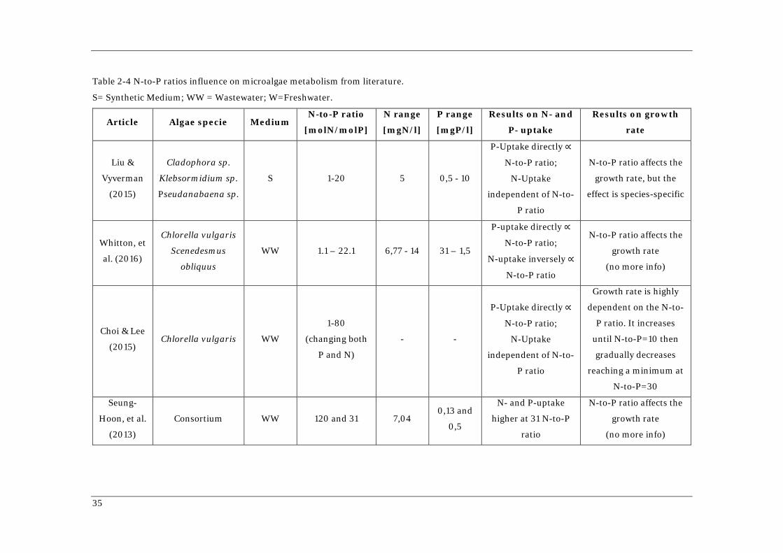
Among the others, the so called the ASM-A model presented by Wágner et al. (2016) was
selected to be used in this work. It was developed to remedy to the issues briefly described
above. Since it has been recently introduced, in the next pages, it is described together with
the Latin Hypercube Sampling based Simplex (LHSS), i.e. the parameters estimations
procedure applied in this work. For more information it is strongly advised to read Wágner et
al. (2016).
2.3.1 ASM-A model
ASM-A was developed as an extension of the well-known Activated Sludge Model ASM-2d
(Henze, et al., 2000). ASM-A only considers green microalgae’s biochemical processes. The
considered processes catalyzed by green microalgae are presented in the Gujer matrix reported
in Table 2-5 and later explained in terms of modeling choices.

40
Table 2-5 The Gujer matrix of ASM-A model (Wágner et al., 2016)
Component NH4 NO3 Internal
quota N
PO4 Internal
quota P
Inorg.
carbon Acetate O2
Algal
Biomass
Inert
Particulates
Slowly
biodegradable
Particulate
R
a
t
e
Symbol SNH4 SNO XAlg,N SPO4 XAlg,PP SAlk SA SO2 XAlg XI XS
Unit gN/m3 gN/m3 gN/m3 gP/m3 gP/m3 g C/m3 gCOD/m3 gCOD/m3 gCOD/m3 gCOD/m3 gCOD/m3
Process Stoichiometric Matrix
Uptake and
storage of
nitrogen from
NH4
-1 1
R1
Uptake and
storage of
nitrogen from
NO3
-1 1
R2
Uptake and
Storage of PO4
-1 1 R3
Autotrophic
growth - iNXalg
-iPXalg -1/YXalg,SAlk 2.67/YXalg,SAlk 1 R4
Heterotrophic
growth - iNXalg
-iPXalg 0.4/YAc -1/YAc 1-1/YAc 1 R5
Decay
iNXalg
- fXI.iNXalgI
- (1-fXI).iNXalgS
iPXalg
- fXI.iPXalgI
- (1-fXI).iPXalgS
-(1-fXI) -1 fXI 1- fXI R6
41
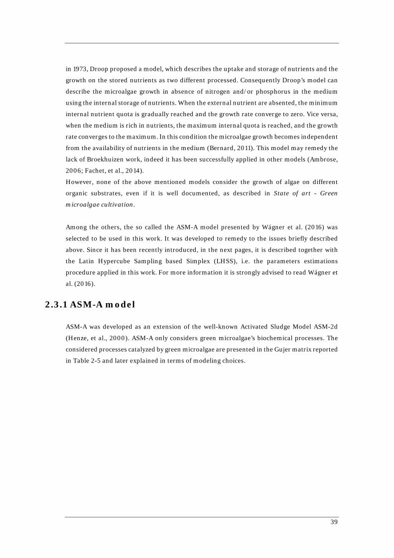
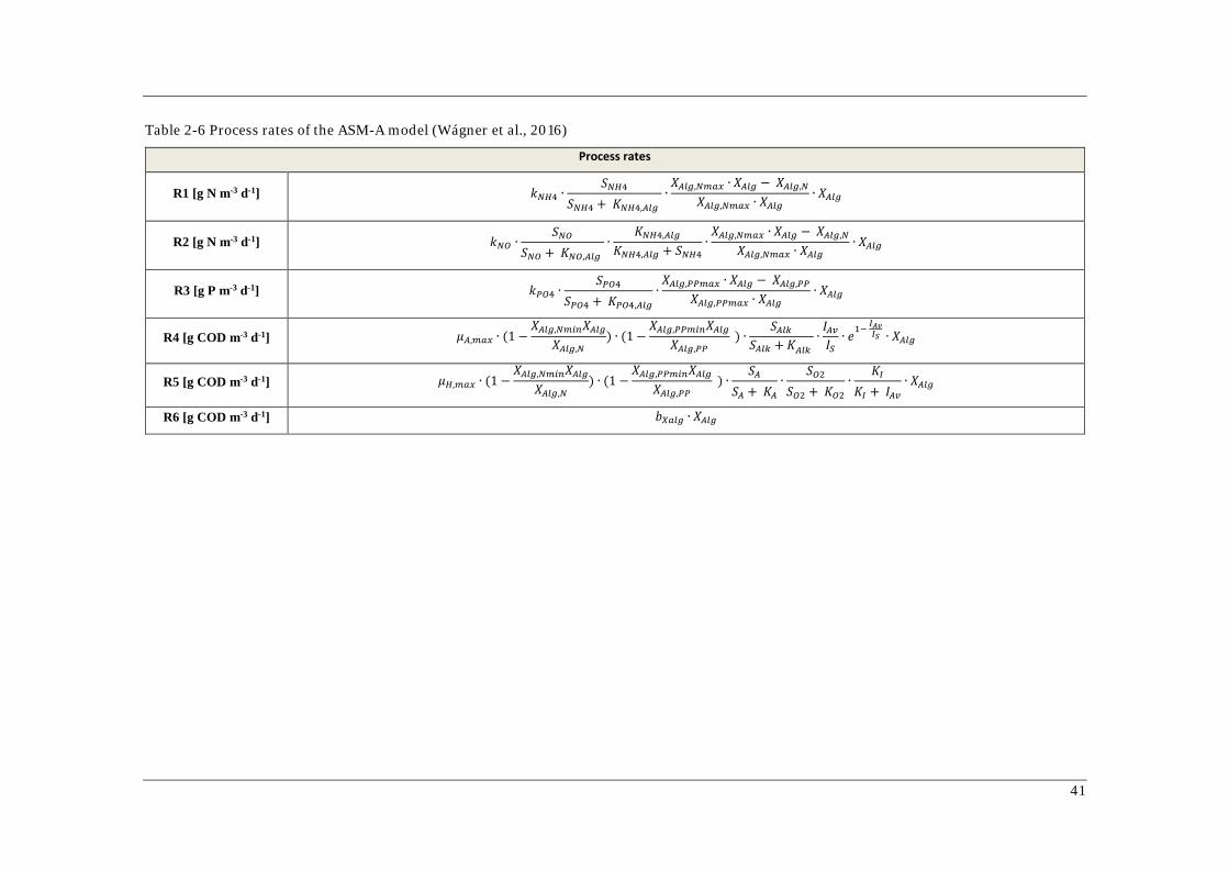
Table 2-6 Process rates of the ASM-A model (Wágner et al., 2016)
Process rates
R1 [g N m-3 d-1] 𝑘𝑘𝑁𝑁𝑁𝑁4 ∙𝑆𝑆𝑁𝑁𝑁𝑁4
𝑆𝑆𝑁𝑁𝑁𝑁4 + 𝐾𝐾𝑁𝑁𝑁𝑁4,𝐴𝐴𝐴𝐴𝐴𝐴 ∙𝑋𝑋𝐴𝐴𝐴𝐴𝐴𝐴,𝑁𝑁𝑁𝑁𝑎𝑎𝑁𝑁 ∙ 𝑋𝑋𝐴𝐴𝐴𝐴𝐴𝐴 − 𝑋𝑋𝐴𝐴𝐴𝐴𝐴𝐴,𝑁𝑁
𝑋𝑋𝐴𝐴𝐴𝐴𝐴𝐴,𝑁𝑁𝑁𝑁𝑎𝑎𝑁𝑁 ∙ 𝑋𝑋𝐴𝐴𝐴𝐴𝐴𝐴∙ 𝑋𝑋𝐴𝐴𝐴𝐴𝐴𝐴
R2 [g N m-3 d-1] 𝑘𝑘𝑁𝑁𝑁𝑁 ∙𝑆𝑆𝑁𝑁𝑁𝑁
𝑆𝑆𝑁𝑁𝑁𝑁 + 𝐾𝐾𝑁𝑁𝑁𝑁,𝐴𝐴𝐴𝐴𝐴𝐴 ∙
𝐾𝐾𝑁𝑁𝑁𝑁4,𝐴𝐴𝐴𝐴𝐴𝐴
𝐾𝐾𝑁𝑁𝑁𝑁4,𝐴𝐴𝐴𝐴𝐴𝐴 + 𝑆𝑆𝑁𝑁𝑁𝑁4∙𝑋𝑋𝐴𝐴𝐴𝐴𝐴𝐴,𝑁𝑁𝑁𝑁𝑎𝑎𝑁𝑁 ∙ 𝑋𝑋𝐴𝐴𝐴𝐴𝐴𝐴 − 𝑋𝑋𝐴𝐴𝐴𝐴𝐴𝐴,𝑁𝑁
𝑋𝑋𝐴𝐴𝐴𝐴𝐴𝐴,𝑁𝑁𝑁𝑁𝑎𝑎𝑁𝑁 ∙ 𝑋𝑋𝐴𝐴𝐴𝐴𝐴𝐴∙ 𝑋𝑋𝐴𝐴𝐴𝐴𝐴𝐴
R3 [g P m-3 d-1] 𝑘𝑘𝑃𝑃𝑁𝑁4 ∙𝑆𝑆𝑃𝑃𝑁𝑁4
𝑆𝑆𝑃𝑃𝑁𝑁4 + 𝐾𝐾𝑃𝑃𝑁𝑁4,𝐴𝐴𝐴𝐴𝐴𝐴∙𝑋𝑋𝐴𝐴𝐴𝐴𝐴𝐴,𝑃𝑃𝑃𝑃𝑁𝑁𝑎𝑎𝑁𝑁 ∙ 𝑋𝑋𝐴𝐴𝐴𝐴𝐴𝐴 − 𝑋𝑋𝐴𝐴𝐴𝐴𝐴𝐴,𝑃𝑃𝑃𝑃
𝑋𝑋𝐴𝐴𝐴𝐴𝐴𝐴,𝑃𝑃𝑃𝑃𝑁𝑁𝑎𝑎𝑁𝑁 ∙ 𝑋𝑋𝐴𝐴𝐴𝐴𝐴𝐴∙ 𝑋𝑋𝐴𝐴𝐴𝐴𝐴𝐴
R4 [g COD m-3 d-1] 𝜇𝜇𝐴𝐴,𝑁𝑁𝑎𝑎𝑁𝑁 ∙ (1 −𝑋𝑋𝐴𝐴𝐴𝐴𝐴𝐴,𝑁𝑁𝑁𝑁𝑁𝑁𝑁𝑁𝑋𝑋𝐴𝐴𝐴𝐴𝐴𝐴
𝑋𝑋𝐴𝐴𝐴𝐴𝐴𝐴,𝑁𝑁) ∙ (1 −
𝑋𝑋𝐴𝐴𝐴𝐴𝐴𝐴,𝑃𝑃𝑃𝑃𝑁𝑁𝑁𝑁𝑁𝑁𝑋𝑋𝐴𝐴𝐴𝐴𝐴𝐴𝑋𝑋𝐴𝐴𝐴𝐴𝐴𝐴,𝑃𝑃𝑃𝑃
) ∙𝑆𝑆𝐴𝐴𝐴𝐴𝐴𝐴
𝑆𝑆𝐴𝐴𝐴𝐴𝐴𝐴 + 𝐾𝐾𝐴𝐴𝐴𝐴𝐴𝐴 ∙𝐼𝐼𝐴𝐴𝐴𝐴𝐼𝐼𝑆𝑆∙ 𝑒𝑒1− 𝐼𝐼𝐴𝐴𝐴𝐴𝐼𝐼𝑆𝑆 ∙ 𝑋𝑋𝐴𝐴𝐴𝐴𝐴𝐴
R5 [g COD m-3 d-1] 𝜇𝜇𝑁𝑁,𝑁𝑁𝑎𝑎𝑁𝑁 ∙ (1 −𝑋𝑋𝐴𝐴𝐴𝐴𝐴𝐴,𝑁𝑁𝑁𝑁𝑁𝑁𝑁𝑁𝑋𝑋𝐴𝐴𝐴𝐴𝐴𝐴
𝑋𝑋𝐴𝐴𝐴𝐴𝐴𝐴,𝑁𝑁) ∙ (1 −
𝑋𝑋𝐴𝐴𝐴𝐴𝐴𝐴,𝑃𝑃𝑃𝑃𝑁𝑁𝑁𝑁𝑁𝑁𝑋𝑋𝐴𝐴𝐴𝐴𝐴𝐴𝑋𝑋𝐴𝐴𝐴𝐴𝐴𝐴,𝑃𝑃𝑃𝑃
) ∙𝑆𝑆𝐴𝐴
𝑆𝑆𝐴𝐴 + 𝐾𝐾𝐴𝐴∙
𝑆𝑆𝑁𝑁2𝑆𝑆𝑁𝑁2 + 𝐾𝐾𝑁𝑁2
∙𝐾𝐾𝐼𝐼
𝐾𝐾𝐼𝐼 + 𝐼𝐼𝐴𝐴𝐴𝐴∙ 𝑋𝑋𝐴𝐴𝐴𝐴𝐴𝐴
R6 [g COD m-3 d-1] 𝑏𝑏𝑋𝑋𝑎𝑎𝐴𝐴𝐴𝐴 ∙ 𝑋𝑋𝐴𝐴𝐴𝐴𝐴𝐴
65
Table 2-7 State variables of ASM-A model (Wágner et al., 2016)
State variables Description Unit
SNH4 Soluble ammonium nitrogen concentration in the bulk liquid g N∙ m-3
SNO Soluble nitrate plus nitrite nitrogen concentration in the bulk liquid g N∙ m-3
SPO4 Inorganic soluble P as ortho-phosphate concentration in the bulk
liquid g P∙ m-3
XAlg,N Internal cell quota of N g N ∙ m-3
XAlg,PP Internal cell quota of P g P ∙ m-3
SAlk Alkalinity consumed via photoautotrophic growth g C∙ m-3
SO2 Dissolved oxygen, produced during photoautotrophic growth and
consumed during heterotrophic growth g COD∙ m-3
SA Fermentation products serving as carbon source for heterotrophic
growth (acetate) g COD∙ m-3
XAlg Algal biomass, produced through growth processes g COD∙ m-3
XI Non - biodegradable inert particulate organic matter g COD∙ m-3
XS Slowly biodegradable particulate organic matter g COD∙ m-3
Table 2-8 Stoichiometric parameters and conversion factors with the initial values used in this study (Wágner et al., 2016)
Stoichiometric parameters
and conversion factors Description Unit
Initial
values
YXalg,SAlk Yield of biomass on alkalinity g COD∙g-1C 2,69
YAc Yield of biomass on acetate g COD∙g-1COD 0,42
iPXalg P content in biomass g P ∙g-1COD 0,0021
iNXalg N content in biomass g N∙ g-1COD 0,00936
fXI Fraction of inert biomass g COD∙g-1COD 0,1
iNXalgI N content of inert particulate COD g N∙g-1COD 0,00431
iNXalgS N content of slowly biodegradable
substrate g N∙g-1COD 0,00495
iPXalgI P content of inert particulate COD g P∙g-1COD 0,00101
iPXalgS P content of slowly biodegradable
substrate g P∙g-1COD 0,00109

43
Table 2-9 Kinetic parameters of ASM-A model with the initial values used in this study (Wágner, 2016)
Kinetic parameters Description Unit Initial values
µA,max Maximum specific photoautotrophic
growth rate
d-1 4,12
µH,max Maximum specific heterotrophic
growth rate
d-1 4,5
Is Light saturation intensity µmol m-2 s-1 758,2
XAlg,PPmin Minimum P cell quota g P∙g-1COD 0,0021
XAlg,Nmin Minimum N cell quota g N∙ g-1COD 0,00936
XAlg,PPmax Maximum P cell quota g P∙ g-1COD 0,016
XAlg,Nmax Maximum N cell quota g N∙ g-1COD 0,13
KNO,Alg Half-saturation coefficient of NO3 g N∙m-3 12,61
KNH4,Alg Half-saturation coefficient of NH4 g N∙m-3 7,87
KPO4,Alg Half-saturation coefficient of PO4 g P∙m-3 4,49
kNH4,Alg Maximum specific uptake rate of
NO3
g N∙g-1COD∙d-1 0,036
kNO,Alg Maximum specific uptake rate of
NH4
g N∙g-1COD∙d-1 0,043
kPO4,Alg Maximum specific uptake rate of
PO4
g P∙g-1COD∙d-1 0,16
KAlk Alkalinity half-saturation coefficient g C∙m-3 3
KA Half-saturation coefficient of acetate gCOD∙m-3 6,3
KI Inhibiting light intensity µmol m-2s-1 331
KO Half-saturation coefficient for
oxygen
gCOD m-3 2
bXalg Decay rate d-1 0,21
Uptake and storage of nitrogen (R1 and R2)
Green microalgae can uptake and store nitrogen from both soluble ammonia (R1) and soluble
nitrate (R2). In both cases the uptake and storage of nitrogen depends on the availability of
nitrogen in the medium (SNH4 or SNO), which is modeled with a Monod kinetic, and on the

Chapter 2 State of art
44
internal cell quota of nitrogen (XAlgN), which limits the nitrogen uptake when it approaches the
maximum internal cell quota (XAlg,Nmax). Moreover, according to Cai, et al. (2013) and Markuo
et al. (2014) green microalgae prefer ammonia over nitrate. Therefore, in the nitrate uptake
process rate, a competitive inhibition term is added.
Uptake and storage of phosphorus (R3)
The uptake and storage of phosphorus (R3) depends on the availability of phosphorus as
soluble orthophosphate in the medium (SPO4), which is modeled with a Monod kinetic, and on
the internal cell quota of phosphorus (XAlgP), which limits the phosphorus uptake when it
approaches the maximum internal cell quota (XAlg,PPmax).
Photoautotrophic growth (R4)
Green microalgae photoautotrophic growth (R4) is based on the availability of internal
nutrients storage, soluble inorganic carbon and light. Thus, the specific growth rate decreases
when the internal cell quota of nitrogen or phosphorus approaches the minimum (XAlg,Nmin or
XAlg,PPmin) and it is modeled according to Droop (1973). The consumption of inorganic carbon
(SAlk) is modeled using Monod kinetics. The light limitation is modeled using the Steele
equation (Steele, 1962).
Heterotrophic algal growth (R5)
Green microalgae heterotrophic growth (R5) is based on the availability of internal nutrients
storage, soluble organic carbon and oxygen. Thus, Monod kinetics are used to model the
heterotrophic growth as function of the organic carbon substrate concentration, i.e. acetate
(SA), and the terminal electron acceptor, i.e. oxygen (SO2). As describe for the photoautotrophic
growth, the specific growth rate decreases when the internal cell quota of nitrogen or
phosphorus approaches the minimum (XAlg,Nmin or XAlg,PPmin). Light limits the heterotrophic
growth, thus it is modeled using a competitive inhibition term.
Alga decay (R6)
The algal decay includes several processes: internal resources used for maintenance, biomass
decreasing during dark respiration, death, lysis, loss of biomass due to predators grazing on
the algal biomass. According to Van Loosdrecht & Henze (1999) the decay process is modeled
following the dead-regeneration principle, which entails the availability of part of the decay
products for microbial growth.
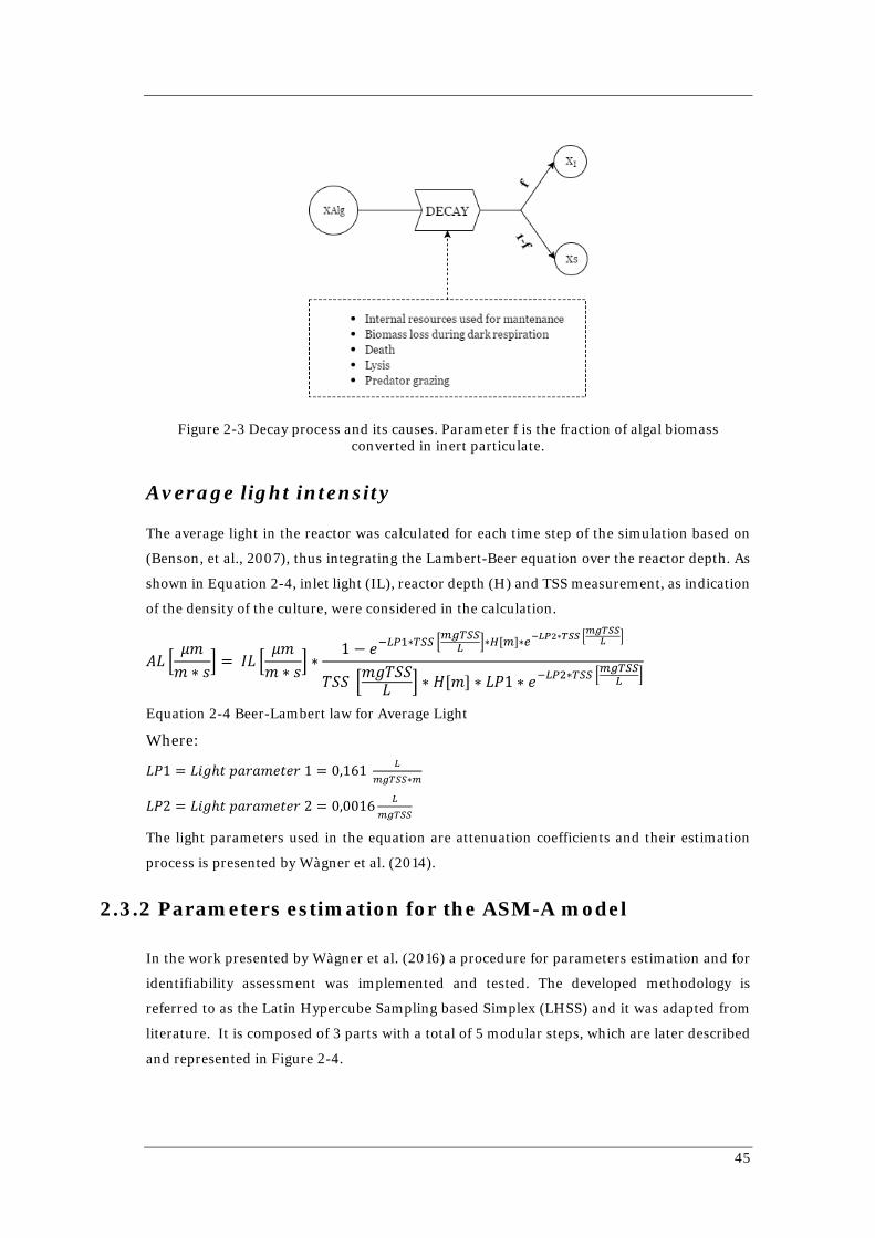
45
Figure 2-3 Decay process and its causes. Parameter f is the fraction of algal biomass converted in inert particulate.
Average light intensity
The average light in the reactor was calculated for each time step of the simulation based on
(Benson, et al., 2007), thus integrating the Lambert-Beer equation over the reactor depth. As
shown in Equation 2-4, inlet light (IL), reactor depth (H) and TSS measurement, as indication
of the density of the culture, were considered in the calculation.
𝐴𝐴𝐴𝐴 �𝜇𝜇𝜇𝜇𝜇𝜇 ∗ 𝑠𝑠�
= 𝐼𝐼𝐴𝐴 �𝜇𝜇𝜇𝜇𝜇𝜇 ∗ 𝑠𝑠�
∗1 − 𝑒𝑒−𝐿𝐿𝑃𝑃1∗𝑇𝑇𝑆𝑆𝑆𝑆 �𝑁𝑁𝐴𝐴𝑇𝑇𝑆𝑆𝑆𝑆
𝐿𝐿 �∗𝑁𝑁[𝑁𝑁]∗𝑒𝑒−𝐿𝐿𝐿𝐿2∗𝑇𝑇𝑆𝑆𝑆𝑆 �𝑚𝑚𝑚𝑚𝑇𝑇𝑆𝑆𝑆𝑆𝐿𝐿 �
𝑇𝑇𝑆𝑆𝑆𝑆 �𝜇𝜇𝑚𝑚𝑇𝑇𝑆𝑆𝑆𝑆𝐴𝐴 � ∗ 𝐻𝐻[𝜇𝜇] ∗ 𝐴𝐴𝐿𝐿1 ∗ 𝑒𝑒−𝐿𝐿𝑃𝑃2∗𝑇𝑇𝑆𝑆𝑆𝑆 �𝑁𝑁𝐴𝐴𝑇𝑇𝑆𝑆𝑆𝑆𝐿𝐿 �
Equation 2-4 Beer-Lambert law for Average Light
Where:
𝐴𝐴𝐿𝐿1 = 𝐴𝐴𝐿𝐿𝑚𝑚ℎ𝑡𝑡 𝑝𝑝𝑝𝑝𝑝𝑝𝑝𝑝𝜇𝜇𝑒𝑒𝑡𝑡𝑒𝑒𝑝𝑝 1 = 0,161 𝐿𝐿𝑁𝑁𝐴𝐴𝑇𝑇𝑆𝑆𝑆𝑆∗𝑁𝑁
𝐴𝐴𝐿𝐿2 = 𝐴𝐴𝐿𝐿𝑚𝑚ℎ𝑡𝑡 𝑝𝑝𝑝𝑝𝑝𝑝𝑝𝑝𝜇𝜇𝑒𝑒𝑡𝑡𝑒𝑒𝑝𝑝 2 = 0,0016 𝐿𝐿𝑁𝑁𝐴𝐴𝑇𝑇𝑆𝑆𝑆𝑆
The light parameters used in the equation are attenuation coefficients and their estimation
process is presented by Wàgner et al. (2014).
2.3.2 Parameters estimation for the ASM-A model
In the work presented by Wàgner et al. (2016) a procedure for parameters estimation and for
identifiability assessment was implemented and tested. The developed methodology is
referred to as the Latin Hypercube Sampling based Simplex (LHSS) and it was adapted from
literature. It is composed of 3 parts with a total of 5 modular steps, which are later described
and represented in Figure 2-4.

Chapter 2 State of art
46
Pre-Calibration
Step 1
Based on a wide literature review in Wágner et al. (2016) a range of possible values for each
parameter was defined. Table 2-10 reports the upper and lower boundaries that define the
ranges for the parameters of interest for this work.
Figure 2-4 Scheme of the LHSS method proposed for parameter estimation and identifiability assessment (Wágner, 2016)

47
Table 2-10 Upper and lower bounds, that define the ranges used during the LHSS calibration process (Wágner, 2016)
Parameter Lower bound Upper bound
µA,max (d-1) 2.5 6.5
KNO,Alg
(gN∙m-3) 0.001 15
KPO4,Alg
(gP∙m-3) 0.001 5
kNO,Alg
(gN∙g1COD∙d-1) 0.001 5
kPO4,Alg
(gP∙g-1COD∙d-1) 0.001 5
bAlg (d-1) 0.01 0.5
Step 2
The first parameters set is selected from the given ranges (Table 2-10) using the Latin
Hypercube Sampling (Helton & Davis, 2003). In this work, 500 first parameters sets were
identified.
Parameter estimation
Step 3
Each parameters set identified in Step 2 is the a priori values used for Simplex (Nelder & Mead,
1965), i.e. local optimization algorithm. It identifies the optimal parameters set, minimizing
the root mean square normalized error (RMSNE) relative to the measured value.
𝑅𝑅𝑅𝑅𝑆𝑆𝑁𝑁𝑅𝑅 = �1𝑛𝑛��
𝑦𝑦𝑁𝑁 − 𝑦𝑦𝑦𝑦𝑁𝑁
�2𝑁𝑁
𝑁𝑁=1
Equation 2-5 RMSNE Equation
Where:
𝑛𝑛 = 𝑛𝑛𝑛𝑛𝜇𝜇𝑏𝑏𝑒𝑒𝑝𝑝 𝑜𝑜𝑜𝑜 𝜇𝜇𝑒𝑒𝑝𝑝𝑠𝑠𝑛𝑛𝑝𝑝𝑝𝑝𝜇𝜇𝑒𝑒𝑛𝑛𝑡𝑡 𝑝𝑝𝑜𝑜𝐿𝐿𝑛𝑛𝑡𝑡𝑠𝑠
𝑦𝑦𝑁𝑁 = 𝜇𝜇𝑒𝑒𝑝𝑝𝑠𝑠𝑛𝑛𝑝𝑝𝑒𝑒𝑚𝑚 𝑣𝑣𝑝𝑝𝑣𝑣𝑛𝑛𝑒𝑒
𝑦𝑦 = 𝑝𝑝𝑝𝑝𝑒𝑒𝑚𝑚𝐿𝐿𝑝𝑝𝑡𝑡𝑒𝑒𝑚𝑚 𝑣𝑣𝑝𝑝𝑣𝑣𝑛𝑛𝑒𝑒𝑠𝑠

Chapter 2 State of art
48
At the end of this operation, 500 optimal parameters sets are defined (one for each a priori
parameters set).
Step 4
The RMSNE distribution is plotted. Considering the minimum error of the distribution a cut-
off value is defined increasing it by the 10%. All the results above the cut-off value is
disregarded. With the remaining sets, the distribution of each parameter is plotted using
histograms. Consequently, for each parameter the mean values and the standard deviations
are calculated. In this way the optimal parameters set is defined.
Figure 2-5 Example of the definition of the cut of value
Identifiability analysis
Step 5
To define the parameters identifiability the following elements are used:
• the distribution of the optimal parameter set values plotted as histograms
• the average parameter values
• the standard deviation
• the correlation matrix
According to Van Daele et al. (2015) the histograms of the optimal parameters set values
obtained are interpreted according to their wideness and the standard deviation is consider as
well for a first assessment of the parameter identifiability. If the histograms are too wide and
the standard deviation relatively too high, the parameter is classified as non-identifiable.
Otherwise, as suggested by Sin et al.(2010), the covariance is checked. If it is comparably low,
the parameter is classified as identifiable. In the opposite case, the parameter identifiability is
assessed by analyzing the difference in the simulation output by setting the parameter to its
minimum and maximum boundaries defined by the standard deviation (Figure 2-6). As
suggest by Sin et al.(2010), to assess the differences in the model predictions the Janus

49
coefficient is used. It describes the accuracy of the model prediction. When its value is close to
1 the model prediction is accurate and thus, the studied parameter is identifiable. Otherwise,
the predictions are worse or better than the original model approximations obtained through
parameter estimation and thus the studied parameter is non-identifiable.
𝐽𝐽𝑝𝑝𝑛𝑛𝑛𝑛𝑠𝑠 𝑝𝑝𝑜𝑜𝑒𝑒𝑜𝑜𝑜𝑜𝐿𝐿𝑝𝑝𝐿𝐿𝑒𝑒𝑛𝑛𝑡𝑡 =𝑅𝑅𝑅𝑅𝑆𝑆𝑁𝑁𝑅𝑅_𝑏𝑏𝑜𝑜𝑛𝑛𝑛𝑛𝑚𝑚𝑝𝑝𝑝𝑝𝑦𝑦𝑅𝑅𝑅𝑅𝑆𝑆𝑁𝑁𝑅𝑅_𝜇𝜇𝑒𝑒𝑝𝑝𝑛𝑛
Equation 2-6 Janus coefficient equation
Where:
RMSNE_boundary = RMSNE calculated on the simulation with the parameter value at the boundary
RMSNE_mean= RMSNE calculated on the simulation with the mean parameter value
Figure 2-6 Diagram of the final process for the identifiability of the parameters


50
MATERIALS AND METHODS
3.1 Laboratory experiments
3.1.1 Green microalgae culture
The mixed green microalgal culture used in these experiments was originally isolated in a
natural pond in contact with wastewater. At that time, the culture mainly consisted of
Chlorella sp. and Scenedesmus sp.. The algal culture grew strictly in suspension, without
significant biofilm or aggregate formation (Wágner, 2016). The mixed culture was cultivated
using the MWC+Se synthetic medium (Guillard & Lorenzen, 1972). Over time, the mixed
culture selected to Chlorella sp. naturally. Therefore, the experiments were carried out with a
monoculture of Chlorella sp..
3.1.2 Experimental design and reactors description
EBRP system
A laboratory scale EBPR system was used to treat wastewater.
The system was originally built as EBP2R system and later converted to a traditional EBPR
system. The system was designed according to the empirical guidelines established by Randall
et al. (1998) for EBPR system. It was built as a sequence of anaerobic-aerobic reactors for a

51
total of two anaerobic reactors, one aerobic reactor and one clarifier. The layout of the plant is
reported in Figure 3-2 while pictures of each reactor can be seen in Figure 3-1.
1. The anaerobic phase was divided into two reactors setup in two glass cylinders with a
working volume of 1,25L and a cap to close the reactor in order to limit oxygen transfer
from air to the liquid phase. A rotational stirrer working at 60 rpm provided mixing.
Differently from the traditional EBPR system, the anaerobic volume was divided in
two different reactor to enhance phosphorus release in the anaerobic phase and thus
to recover more phosphorus from the P-stream in the EBP2R (Valverde-Pérez, 2015).
This feature wasn’t changed when the system has been converted to EBPR.
2. The aerobic phase consisted of a 5.8L glass cylinder. Air was provided from the
bottom of the reactor by an air diffuser and a rotational stirrer working at 85 rpm
provided mixing.
3. The clarifier was a 2L glass reactor with a cylinder part for settling and a hopper in
the bottom.
1. Anaerobic reactors 2. Aerobic reactor 3. Clarifier
Figure 3-1 Pictures of the main components of the laboratory scale EBPR system
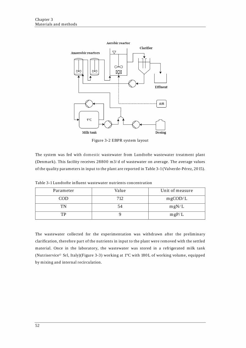
Chapter 3 Materials and methods
52
Figure 3-2 EBPR system layout
The system was fed with domestic wastewater from Lundtofte wastewater treatment plant
(Denmark). This facility receives 28800 m3/d of wastewater on average. The average values
of the quality parameters in input to the plant are reported in Table 3-1 (Valverde-Pérez, 2015).
Table 3-1 Lundtofte influent wastewater nutrients concentration
Parameter Value Unit of measure
COD 712 mgCOD/L
TN 54 mgN/L
TP 9 mgP/L
The wastewater collected for the experimentation was withdrawn after the preliminary
clarification, therefore part of the nutrients in input to the plant were removed with the settled
material. Once in the laboratory, the wastewater was stored in a refrigerated milk tank
(Nutriservice© Srl, Italy)(Figure 3-3) working at 1°C with 180L of working volume, equipped
by mixing and internal recirculation.
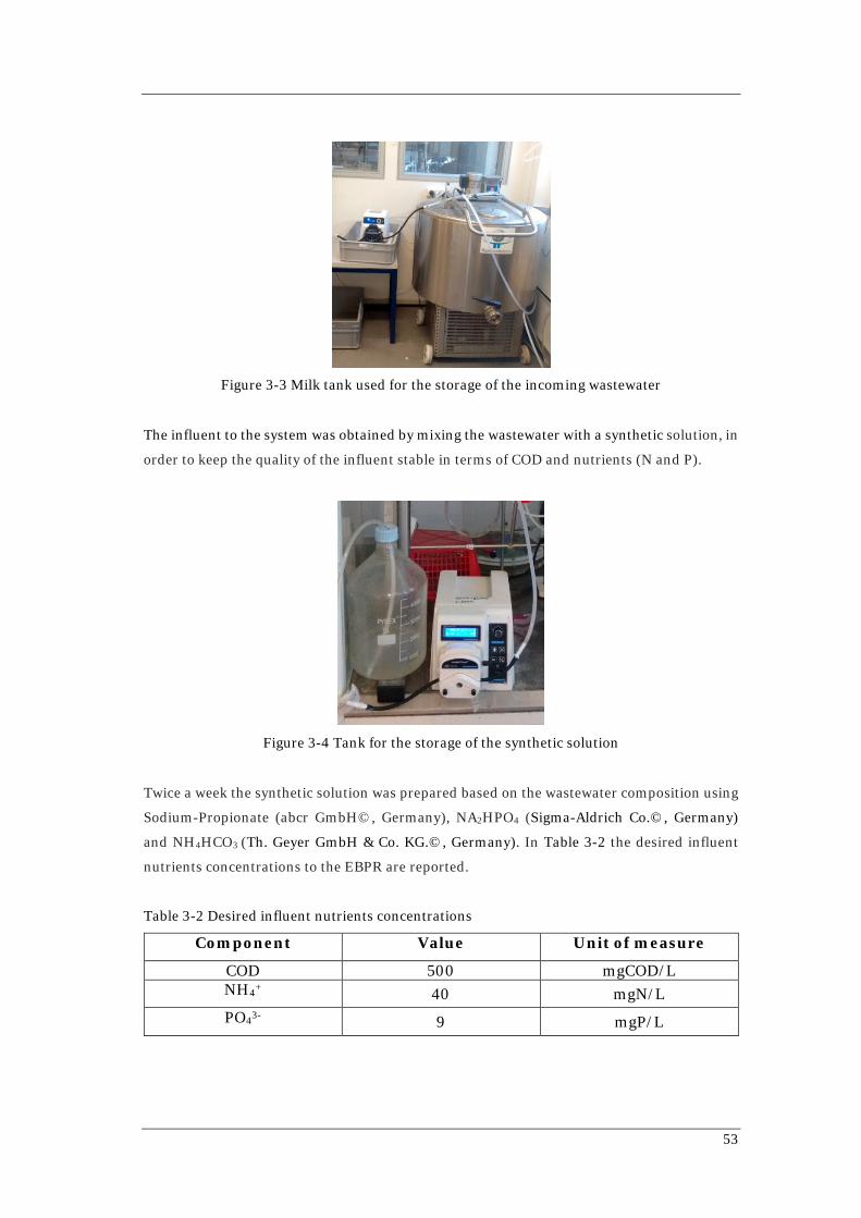
53
Figure 3-3 Milk tank used for the storage of the incoming wastewater
The influent to the system was obtained by mixing the wastewater with a synthetic solution, in
order to keep the quality of the influent stable in terms of COD and nutrients (N and P).
Figure 3-4 Tank for the storage of the synthetic solution
Twice a week the synthetic solution was prepared based on the wastewater composition using
Sodium-Propionate (abcr GmbH©, Germany), NA2HPO4 (Sigma-Aldrich Co.©, Germany)
and NH4HCO3 (Th. Geyer GmbH & Co. KG.©, Germany). In Table 3-2 the desired influent
nutrients concentrations to the EBPR are reported.
Table 3-2 Desired influent nutrients concentrations
Component Value Unit of measure
COD 500 mgCOD/L NH4+ 40 mgN/L PO43- 9 mgP/L

Chapter 3 Materials and methods
54
The HRT in the system was kept to 13,8h with an inflow of 11,1L/day. As a traditional EBPR
system, recirculation of sludge from the clarifier to the first anaerobic reactor was provided.
Moreover part of the sludge was daily discharged from the aerobic reactor, thus total SRT was
kept at 16 days. Peristaltic pumps were used to maintain the flows in the system.
Continuous flow PBRs
Two PBRs were run in parallel downstream to the laboratory scale EPBR system. They were
setup using two glass cylinders with a working volume of 1,4 L (Figure 3-5). The system was
built under a fume hood to reduce risk of unwanted contamination and to keep surrounding
environmental conditions stable (T~20°C).
Figure 3-5 Picture of the two parallel photobioreactors
Continuous lighting was provided by a custom-built lamp, providing an average of 1250 µmol
photons m-2 s-1, with one metal-halide light bulb (OSRAM©, Germany), which simulates the
solar spectrum, from the top of the reactor and a black sheet was used to cover the lateral
surface of the cylinder, so it received light only from the top (Figure 3-6).

55
Figure 3-6 Picture of the two parallel photobioreactors covered with a black sheet and the lamps on the top
CO2 enriched airflow was supplied from the bottom of the reactor by an air hose diffuser to
guarantee CO2 supply and full mixing. Mixing allowed maintaining homogeneous conditions
along the reactor and equal light exposure to algae. CO2 dissolution was used to keep pH inside
the reactor at neutral values (range 6,10-7,9). For this purpose, the airflow and the %vol of
CO2 were manually adjusted every day(30%±10 for the %vol of CO2). Inlet light and pH were
monitored using LI-1400 Data Logger with LI-193 Spherical Underwater Quantum Sensor
(2016LI-COR©, USA)(Figure 3-7) and Multi 3430 Digital pH meter for pH-Electrode Sentix
940 sensor ( 2016 WTW Wissenschaftlich-Technische Werkstätten GmbH. ©, Germany),
respectively.
Figure 3-7 Light sensor
Influent streams were provided from the bottom of the reactors by a peristaltic pump (BT100-
1F) with two pump head (Longer Precision Pump Co., China), which guarantee 243 µm/min
flow to each reactor. Thus the SRT=HRT was kept at 3,5 days. Each pump heads withdrew the
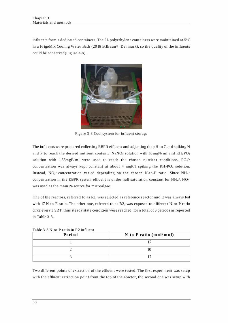
Chapter 3 Materials and methods
56
influents from a dedicated containers. The 2L polyethylene containers were maintained at 5°C
in a FrigoMix Cooling Water Bath (2016 B.Braun©, Denmark), so the quality of the influents
could be conserved(Figure 3-8).
Figure 3-8 Cool system for influent storage
The influents were prepared collecting EBPR effluent and adjusting the pH to 7 and spiking N
and P to reach the desired nutrient content. NaNO3 solution with 10mgN/ml and KH2PO4
solution with 1,55mgP/ml were used to reach the chosen nutrient conditions. PO43-
concentration was always kept constant at about 4 mgP/l spiking the KH2PO4 solution.
Instead, NO3- concentration varied depending on the chosen N-to-P ratio. Since NH4+
concentration in the EBPR system effluent is under half saturation constant for NH4+, NO3-
was used as the main N-source for microalgae.
One of the reactors, referred to as R1, was selected as reference reactor and it was always fed
with 17 N-to-P ratio. The other one, referred to as R2, was exposed to different N-to-P ratio
circa every 3 SRT, thus steady state condition were reached, for a total of 3 periods as reported
in Table 3-3.
Table 3-3 N-to-P ratio in R2 influent Period N-to-P ratio (mol/mol)
1 17
2 10
3 17
Two different points of extraction of the effluent were tested. The first experiment was setup
with the effluent extraction point from the top of the reactor, the second one was setup with

57
the effluent extraction point from the half height of the reactor. As explained in Results and
Discussion - System layout: the problem and the solution the second layout, represented in
Figure 3-9 , was chosen.
Figure 3-9 Layout of continuous flow PBRs system
1-L Batch experiment
One batch experiment was set up with 1-L wide-neck glass bottle (2014Duran©, Germany)
equipped by a multi-port system (Figure 3-10), allowing for sample extraction and aeration
with 10 L/h CO2 enriched air (5% CO2), which guarantees CO2 supply. Mixing was provided
by a magnetic stirrer at 180 rpm to maintain equal conditions along the reactor and equal light
exposure to algae. Continuous lighting was radiated by one 80-W GroLux fluorescent lamp
(2013 Osram Sylvania©, USA), which simulates the solar spectrum, located on one side of the
reactor, which provided an average light intensity of 150 µmol/(m2*s). The temperature of the
environment was maintained at 20°C thanks to the air conditioning system implemented in
the laboratory where the experiment was carried out. pH remained around neutral values.

Chapter 3 Materials and methods
58
Figure 3-10 Batch experiment layout and photo
The batch was prepared using 800ml of effluent from the pilot scale EBPR system and 200 ml
of Chlorella sp. culture. The experiment was run with an initial N-to-P ratio of about 17
mol/mol and an initial concentration of PO3- of about 4 mgP/L . This condition was reached
spiking NH4KCO3 solution and KH2PO4 solution (1,55 gP/ml). In Table 3-4 the initial
concentration of nutrients and total suspend solids are reported.
Table 3-4 Initial condition in 1-L Batch experiment
NH4+ NO3- NO2- PO43- TSS
[mgN/l] [mgN/l] [mgN/l] [mgP/l] [g/l]
14,8 11,2 0,42 3,07 0,057
It is important to notice that, at starting point, there were two main N-source available for the
culture, NH4+ and NO3-. This will have an effect on the uptake of nutrients, which will be
describe in Results and Discussion - Implication on N-source.
The experiment was run until stable concentration for NH4+, NO3- and PO43- were reached.
1.2 L batch experiments
Two batch experiments were setup using a glass cylinder with a working volume of 1,2 L
(Figure 3-11). A black sheet was used to cover the lateral surface of the cylinder, so it received
light only from the top. Continuous lighting was provided by one custom-built lamp with one
metal-halide light bulbs (2016 OSRAM©, Germany), which simulates the solar spectrum, from
the top of the reactor with an average ligth intensity of 1000 µmol/(m2*s). CO2 enriched
airflow was supplied from the bottom of the reactor by an air hose diffuser to guarantee CO2
supply and full mixing. Mixing allowed maintaining equal conditions along the reactor and
equal light exposure to algae. Moreover, CO2 dissolution was used to keep pH at neutral values
between 6.5 and 7.5. For this purpose, the airflow and the %vol of CO2 were manually adjusted

59
every day(30%±10 for the %vol of CO2). The system was built under a fume hood to reduce
risk of unwanted contamination and to keep surrounding environmental conditions stable
(T~20). Incoming light intensity and pH were monitored using LI-1400 Data Logger with LI-
193 Spherical Underwater Quantum Sensor (2016 LI-COR©, USA) and Multi 3430 Digital pH
meter for pH-Electrode Sentix 940 sensor (2016 WTW Wissenschaftlich-Technische
Werkstätten GmbH. ©, Germany), respectively.
Figure 3-11 Batch experiment layout and photo
The batch was prepared using 1 L of effluent from the pilot scale EBPR system and 200 ml of
effluent from the second PBR containing Chlorella sp. culture. Both experiments were run
with an initial N-to-P ratio of 17 mol/mol and an initial concentration of PO3- of about 4
mgP/L. This condition was reached spiking NaNO3 solution (10mgN/ml) and KH2PO4
solution (1,55 mgP/ml). The difference between the two experiments was the history of the
culture. The first batch was prepared using the effluent of the second PBR (R2) collected
during the first period, thus the Chlorella sp. culture was exposed for a long period to 17
mol/mol N-to-P ratio circa. Instead, the second batch was prepared using the effluent of the
second PBR collected during the second period, thus the Chlorella sp. culture was exposed for
a long period to 10 mol/mol N-to-P ratio circa.
The two experiments were run until nutrients concentrations (NO3-, PO43-) were depleted.

Chapter 3 Materials and methods
60
3.1.3 Analytical methods
Biomass
Biomass in the reactors was analysed by total suspended solids measurement (TSS) and by
measuring the optical density (OD) at 750 nm.
TSS was measured filtering the suspension using glass fiber filter Advantec® GA-55 with pore
size of 0.6 µm (Frisenette ApS, Denmark) and drying them following the standard methods.
OD was measured using microtiter plates filled with 2mL of sample and analysing them with
SynergyMX Multi-Mode Microplate Reader (2016 BioTek Instruments Inc. ©, Winooski)
(Figure 3-12).
Figure 3-12 SynergyMX Multi-MOde Microplate Reader (©2016 BioTek Instruments Inc.)
Nutrients and COD
Total nitrogen (TN), total phosphorus (TP) and chemical oxygen demand (COD) were
measured in algal suspension using commercial test kits (Hach-Lange©, USA).
Ammonium (NNH4+), nitrate (NNO3-), nitrite (NNO2-) and phosphate (PPO43-) concentrations were
measured in filtered samples using test kits supplied by Merck© (USA).
Total soluble nitrogen (TSN) and soluble chemical oxygen demand (sCOD) were measured in
filtered samples using commercial test kits (Hach-Lange©, USA).
Filtration was carried out using glass fiber filter Advantec® GA-55 with pore size of 0.6 µm
(Frisenette ApS, Denmark) followed by a second filtration with 0.2 µm Minisart® NML
disposable filter (©2016 Th. Geyer GmbH & CO- KG., Germany).
The algal biomass was calculated converting TSS units in to COD using a conversion factor of
0,89 gTSS/gCOD estimated from the data collection for the studied microalgae culture.
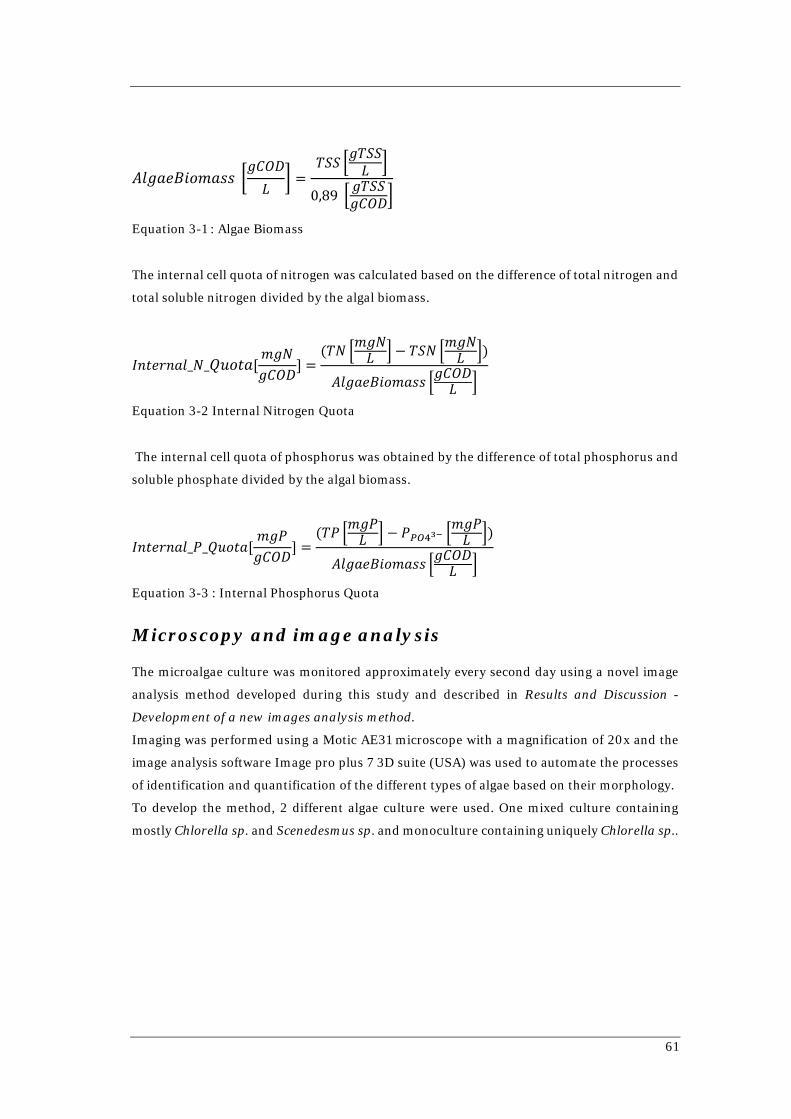
61
𝐴𝐴𝑣𝑣𝑚𝑚𝑝𝑝𝑒𝑒𝐴𝐴𝐿𝐿𝑜𝑜𝜇𝜇𝑝𝑝𝑠𝑠𝑠𝑠 �𝑚𝑚𝐶𝐶𝐶𝐶𝑔𝑔𝐴𝐴
� =𝑇𝑇𝑆𝑆𝑆𝑆 �𝑚𝑚𝑇𝑇𝑆𝑆𝑆𝑆𝐴𝐴 �
0,89 � 𝑚𝑚𝑇𝑇𝑆𝑆𝑆𝑆𝑚𝑚𝐶𝐶𝐶𝐶𝑔𝑔�
Equation 3-1 : Algae Biomass
The internal cell quota of nitrogen was calculated based on the difference of total nitrogen and
total soluble nitrogen divided by the algal biomass.
𝐼𝐼𝑛𝑛𝑡𝑡𝑒𝑒𝑝𝑝𝑛𝑛𝑝𝑝𝑣𝑣_𝑁𝑁_𝑄𝑄𝑛𝑛𝑜𝑜𝑡𝑡𝑝𝑝[𝜇𝜇𝑚𝑚𝑁𝑁𝑚𝑚𝐶𝐶𝐶𝐶𝑔𝑔
] =(𝑇𝑇𝑁𝑁 �𝜇𝜇𝑚𝑚𝑁𝑁𝐴𝐴 � − 𝑇𝑇𝑆𝑆𝑁𝑁 �𝜇𝜇𝑚𝑚𝑁𝑁𝐴𝐴 �)
𝐴𝐴𝑣𝑣𝑚𝑚𝑝𝑝𝑒𝑒𝐴𝐴𝐿𝐿𝑜𝑜𝜇𝜇𝑝𝑝𝑠𝑠𝑠𝑠 �𝑚𝑚𝐶𝐶𝐶𝐶𝑔𝑔𝐴𝐴 �
Equation 3-2 Internal Nitrogen Quota
The internal cell quota of phosphorus was obtained by the difference of total phosphorus and
soluble phosphate divided by the algal biomass.
𝐼𝐼𝑛𝑛𝑡𝑡𝑒𝑒𝑝𝑝𝑛𝑛𝑝𝑝𝑣𝑣_𝐿𝐿_𝑄𝑄𝑛𝑛𝑜𝑜𝑡𝑡𝑝𝑝[𝜇𝜇𝑚𝑚𝐿𝐿𝑚𝑚𝐶𝐶𝐶𝐶𝑔𝑔
] =(𝑇𝑇𝐿𝐿 �𝜇𝜇𝑚𝑚𝐿𝐿𝐴𝐴 � − 𝐿𝐿𝑃𝑃𝑁𝑁43− �
𝜇𝜇𝑚𝑚𝐿𝐿𝐴𝐴 �)
𝐴𝐴𝑣𝑣𝑚𝑚𝑝𝑝𝑒𝑒𝐴𝐴𝐿𝐿𝑜𝑜𝜇𝜇𝑝𝑝𝑠𝑠𝑠𝑠 �𝑚𝑚𝐶𝐶𝐶𝐶𝑔𝑔𝐴𝐴 �
Equation 3-3 : Internal Phosphorus Quota
Microscopy and image analysis
The microalgae culture was monitored approximately every second day using a novel image
analysis method developed during this study and described in Results and Discussion -
Development of a new images analysis method.
Imaging was performed using a Motic AE31 microscope with a magnification of 20x and the
image analysis software Image pro plus 7 3D suite (USA) was used to automate the processes
of identification and quantification of the different types of algae based on their morphology.
To develop the method, 2 different algae culture were used. One mixed culture containing
mostly Chlorella sp. and Scenedesmus sp. and monoculture containing uniquely Chlorella sp..

Chapter 3 Materials and methods
62
3.2 Microalgae modelling and parameters estimation
All the data collected through the laboratory experiments were used in the ASM-A model
presented by Wágner et al. (2016) to assess the goodness of the fit obtained with the parameter
values by Wágner et al. (2016) and to estimate the most significant parameters for this study.
In order to work with the model and the parameters estimation procedure, MATLAB® and
Simulink were used.
The parameters chosen for the estimation are reported in Table 3-5. They were chosen because
they were considered the critical ones, which should show the effect on the green microalgae
kinetics sought in this work.
Table 3-5 Parameters chosen to be estimated in this work
Parameters Description Unit
µA,max (d-1) Maximum specific photoautotrophic growth rate d-1
KNO,Alg
(gN∙m-3) Half-saturation coefficient of NO3 g N∙m-3
KPO4,Alg
(gP∙m-3) Half-saturation coefficient of PO4 g P∙m-3
kNO,Alg
(gN∙g1COD∙d-1) Maximum specific uptake rate of NH4 g N∙g-1COD∙d-1
kPO4,Alg
(gP∙g-1COD∙d-1) Maximum specific uptake rate of PO4 g P∙g-1COD∙d-1
bAlg (d-1) Decay rate d-1


63
RESULTS AND DISCUSSION
The experiments and the analysis described in this chapter were carried out at the department
of Environmental Engineering at Technical University of Denmark. The experimental setup
described in Materials and methods - Laboratory experiments was used to study the impact
of changes in nutrients content in the photobioreactor’s influent on the green microalgae
culture, on the processes involved and on the efficiency in terms of nutrients removal.
4.1 EBPR system: wastewater pre-treatment
In order to use the wastewater from Lundtofte WWTP for the experiments, it was necessary to
treat it. Indeed, the water used for experiments should resemble as much as possible the inlet
water to the PBR in TRENS. A laboratory scale EBPR system was used for this purpose. It was
already working when the laboratory activities for this study began and it was run for the entire
period of work, i.e. around 130 days.
As reported in Materials and methods - EBRP system, the nutrients concentrations in input
to the system were regulated adding a synthetic solution containing Sodium-Propionate
NA2HPO4 and NH4HCO3. In the following charts (Figure 4-1,Figure 4-2 and Figure 4-3) the
weekly concentrations of COD, NH4+ and PO43- are reported and compared to the target
concentrations in input to the EBPR system.

Chapter 4 Results and Discussion
64
Figure 4-1 Measured COD and sCOD influent concentrations
Figure 4-2 Actual NH4+ influent concentration
Figure 4-3 Actual PO43- influent concentration
0100200300400500600700800900
0,0 20,0 40,0 60,0 80,0 100,0 120,0 140,0
[mg/
l]
[day]
COD and sCOD
Target Influent concentration CODInfluent concentration sCODInfluent concentration COD
0
10
20
30
40
50
60
0,0 20,0 40,0 60,0 80,0 100,0 120,0 140,0
[mgN
/l]
[day]
NH4+
Target Influent concentration
Influent concentration
02468
10121416
0 20 40 60 80 100 120 140
[mgP
/l]
[day]
PO43-
Target Influent concentration
Influent concentration

65
From the charts it is possible to see that the input concentrations were kept almost constant
and at the level of the target concentrations. Only the COD shows higher deviation from the
desired target concentration. This is probably resulting from the fact that, to prepare the
synthetic solution, the COD present in the wastewater taken form the WWTP of Lundtofte was
not measured, but it was assumed to be 280 mg/l. Therefore, the correction with the synthetic
solution may have been occasionally incorrect.
Nevertheless, the operation of the system has never been deeply compromised.
The main consequence found was the increasing of the phosphate concentration in the effluent
of the system in response to the lower concentration of COD supplied in input, due to the lack
of carbon source that limits PAOs activity. But this activity was recovered once the COD of the
influent was recovered.
Figure 4-4 Dependence of phosphorus effluent concentration on the influent concentration
of COD
The average efficiencies of the system in the removal of COD, inorganic soluble nitrogen and
phosphate were respectively 93,7%, 66,4% and 81,1%. In Table 4-1 the average nutrients
concentrations in the effluent are reported.
These values are relevant, because they characterize the water used in the experiment with
green microalgae.
00,5
11,5
22,5
33,5
4
0 100 200 300 400 500 600 700 800 900
[mgP
/l]
[mgCOD/l]
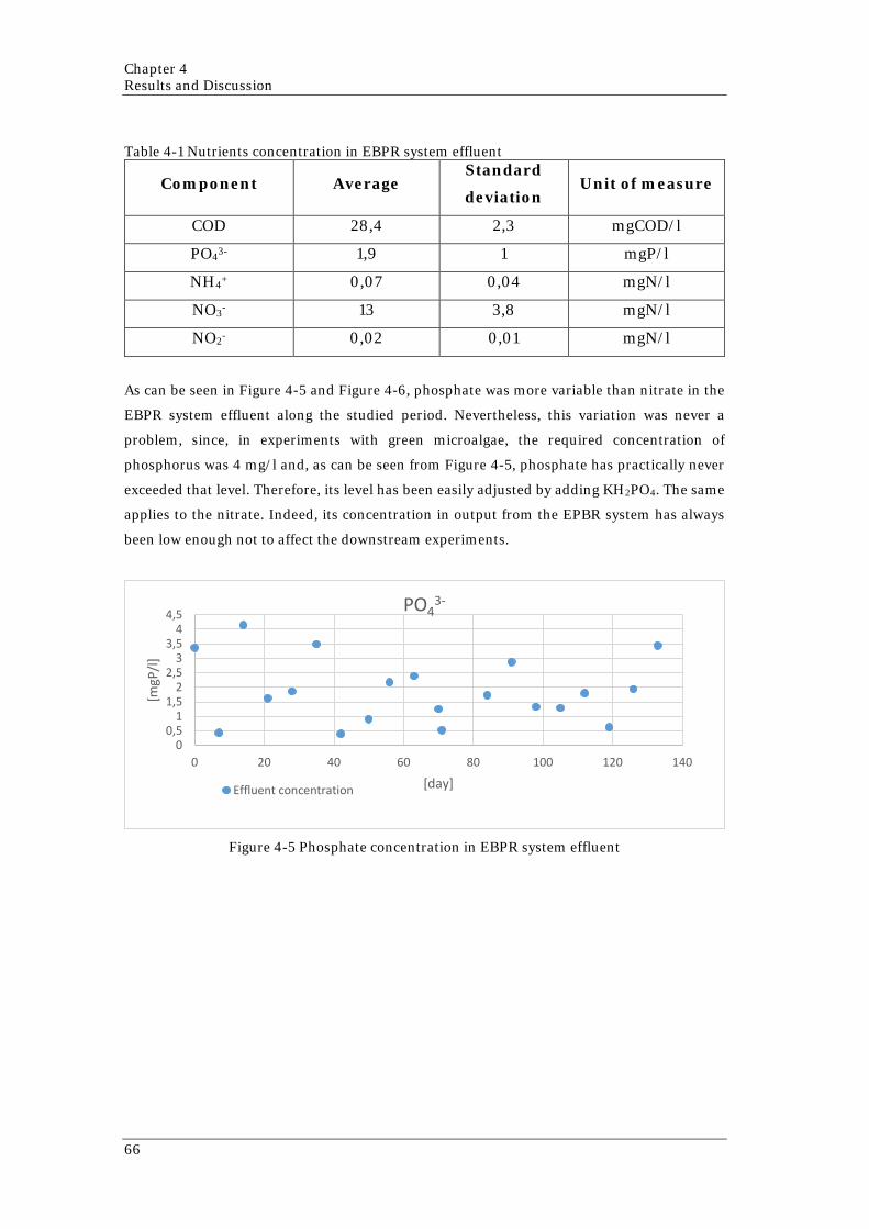
Chapter 4 Results and Discussion
66
Table 4-1 Nutrients concentration in EBPR system effluent
Component Average Standard
deviation Unit of measure
COD 28,4 2,3 mgCOD/l
PO43- 1,9 1 mgP/l
NH4+ 0,07 0,04 mgN/l
NO3- 13 3,8 mgN/l
NO2- 0,02 0,01 mgN/l
As can be seen in Figure 4-5 and Figure 4-6, phosphate was more variable than nitrate in the
EBPR system effluent along the studied period. Nevertheless, this variation was never a
problem, since, in experiments with green microalgae, the required concentration of
phosphorus was 4 mg/l and, as can be seen from Figure 4-5, phosphate has practically never
exceeded that level. Therefore, its level has been easily adjusted by adding KH2PO4. The same
applies to the nitrate. Indeed, its concentration in output from the EPBR system has always
been low enough not to affect the downstream experiments.
Figure 4-5 Phosphate concentration in EBPR system effluent
00,5
11,5
22,5
33,5
44,5
0 20 40 60 80 100 120 140
[mgP
/l]
[day]
PO43-
Effluent concentration

67
Figure 4-6 Nitrate concentration in EBPR system effluent
4.2 1-L Batch
In the following paragraphs the results from the batch run as described in Materials and
methods - 1-L Batch experiment are reported.
4.2.1 Preliminary assessment of ASM-A model performance
As previously mentioned, one of the aims of this work was to test and improve the ASM-A
model, which was described by Wágner et al. (2016). The model was calibrated initially in
Wágner et al. (2016) using synthetic medium, however in this study effluent wastewater was
used and it is expected that the parameters would change depending on the growth medium
used.
Since in Wágner et al. (2016) the calibration of the m0del was carried out using data related
to a mixed culture of Chlorella sp. and Scenedesmus sp., a preliminary test on the performance
of the model for the new culture, which was a monoculture of Chlorella sp., was needed.
Therefore, the data collected during the 1-L Batch experiment were used to assess the
performance of the ASM-A model comparing them with the model prediction. The simulation
was run inserting the initial conditions and boundary conditions of this experiment, which are
presented in Materials and methods - 1-L Batch experiment.
02468
1012141618
0,0 20,0 40,0 60,0 80,0 100,0 120,0 140,0
[mgN
/l]
[day]
NO3-
Effluent concentration
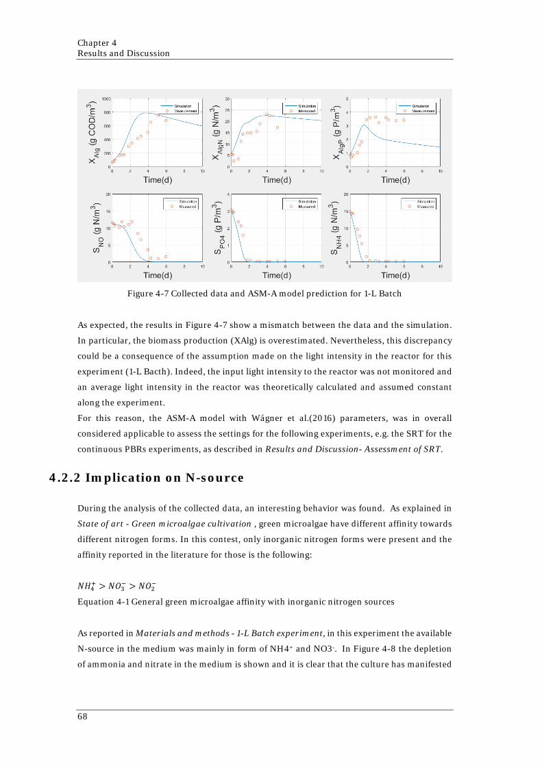
Chapter 4 Results and Discussion
68
Figure 4-7 Collected data and ASM-A model prediction for 1-L Batch
As expected, the results in Figure 4-7 show a mismatch between the data and the simulation.
In particular, the biomass production (XAlg) is overestimated. Nevertheless, this discrepancy
could be a consequence of the assumption made on the light intensity in the reactor for this
experiment (1-L Bacth). Indeed, the input light intensity to the reactor was not monitored and
an average light intensity in the reactor was theoretically calculated and assumed constant
along the experiment.
For this reason, the ASM-A model with Wágner et al.(2016) parameters, was in overall
considered applicable to assess the settings for the following experiments, e.g. the SRT for the
continuous PBRs experiments, as described in Results and Discussion- Assessment of SRT.
4.2.2 Implication on N-source
During the analysis of the collected data, an interesting behavior was found. As explained in
State of art - Green microalgae cultivation , green microalgae have different affinity towards
different nitrogen forms. In this contest, only inorganic nitrogen forms were present and the
affinity reported in the literature for those is the following:
𝑁𝑁𝐻𝐻4+ > 𝑁𝑁𝐶𝐶3− > 𝑁𝑁𝐶𝐶2−
Equation 4-1 General green microalgae affinity with inorganic nitrogen sources
As reported in Materials and methods - 1-L Batch experiment, in this experiment the available
N-source in the medium was mainly in form of NH4+ and NO3-. In Figure 4-8 the depletion
of ammonia and nitrate in the medium is shown and it is clear that the culture has manifested
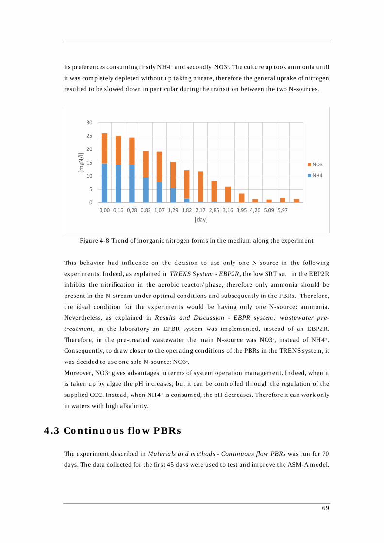
69
its preferences consuming firstly NH4+ and secondly NO3-. The culture up took ammonia until
it was completely depleted without up taking nitrate, therefore the general uptake of nitrogen
resulted to be slowed down in particular during the transition between the two N-sources.
Figure 4-8 Trend of inorganic nitrogen forms in the medium along the experiment
This behavior had influence on the decision to use only one N-source in the following
experiments. Indeed, as explained in TRENS System - EBP2R, the low SRT set in the EBP2R
inhibits the nitrification in the aerobic reactor/phase, therefore only ammonia should be
present in the N-stream under optimal conditions and subsequently in the PBRs. Therefore,
the ideal condition for the experiments would be having only one N-source: ammonia.
Nevertheless, as explained in Results and Discussion - EBPR system: wastewater pre-
treatment, in the laboratory an EPBR system was implemented, instead of an EBP2R.
Therefore, in the pre-treated wastewater the main N-source was NO3-, instead of NH4+.
Consequently, to draw closer to the operating conditions of the PBRs in the TRENS system, it
was decided to use one sole N-source: NO3-.
Moreover, NO3- gives advantages in terms of system operation management. Indeed, when it
is taken up by algae the pH increases, but it can be controlled through the regulation of the
supplied CO2. Instead, when NH4+ is consumed, the pH decreases. Therefore it can work only
in waters with high alkalinity.
4.3 Continuous flow PBRs
The experiment described in Materials and methods - Continuous flow PBRs was run for 70
days. The data collected for the first 45 days were used to test and improve the ASM-A model.
0
5
10
15
20
25
30
0,00 0,16 0,28 0,82 1,07 1,29 1,82 2,17 2,85 3,16 3,95 4,26 5,09 5,97
[mgN
/l]
[day]
NO3
NH4

Chapter 4 Results and Discussion
70
Instead, the data collected in the following days unfortunately resulted to be not usable,
because the cooling system of the reactors did not succeed to maintain 20 °C for a relatively
long period and the ASM-A model does not consider the temperature as a variable.
In the following paragraphs, the work on this experiment is reported and the results obtained
during the first 45 days are described.
4.3.1 Assessment of SRT
Before starting the experiment, different simulations of the experiment using the ASM-A
model were run to assess the feasibility of the experiment and to decide one of the most
important parameters: the SRT. The simulations were run only for R2, because it is the one
subjected to the changing in the influent nutrients concentrations and therefore it was
considered as the critical one. The simulations were set using:
1) the set of parameters calibrated in Wágner et al. (2016);
2) the initial condition expected based on the green microalgae culture in our possession
and the typical concentrations in the effluent of the EBPR system, with which the
culture would have been diluted to fill the reactors;
3) the sequence of inputs expected for the experiment according to Materials and
methods - Continuous flow PBRs.
The simulations were run with different SRT, so that an optimal SRT could be identified. The
idea was to find the lowest SRT possible that allowed to keep a certain level of biomass in the
reactors avoiding algal washout and to reach a good level of nutrients removal.
SRT = 3,5 days was identified as the optimal one. In Figure 4-9 the results of the simulation
for R2 with 3,5 days and 1 day as SRT are shown. In the first case the biomass is kept around
500 gCOD/m3 along the experiment, therefore no washout appears. At the same time, the
removal of nitrogen and phosphorus obtained reaches an acceptable level. In the second case,
the biomass is too reduce (around 40 gCOD/m3) and consequently the removal of nitrogen
and phosphorus is not sufficient.

71
SRT=
3,5
days
SRT=
1 da
y
Figure 4-9 Results of the simulation of R2 using SRT=3,5 days (above) and using SRT=1 day
(below)
4.3.2 System layout: the problem and the solution
As previously mentioned in Materials and methods - Continuous flow PBRs two system
layout were tested. Firstly, the experiment was started with the effluent extraction point on the
top of the reactors as shown in Figure 4-10.

Chapter 4 Results and Discussion
72
Figure 4-10 System layout 1: Effluent extraction point on the top of the reactor
Using this layout, it was clear that something was not right, because the biomass in the reactors
was decreasing, in spite of what was expected based on the simulations previously done. After
15 days, the algae biomass was so reduced and weakened (from 0,1 gTSS/l at Day 1 to 0,02
gTSS/l at Day 15) that other microorganisms (Figure 4-11) contaminated the reactors.
Figure 4-11 Picture of the culture that shows the contamination
Since at that moment the causes were not clear, the experiment was started again with the
same setting. In less than 24 hours from the beginning of the experiment, the loss of biomass
in both reactors was so pronounced that it was clear that the biomass was washed out from the
reactors through the effluent (Table 4-2). In R2, from Day 1 to Day 2 around 0,26 g of biomass
was washed out and the same happened in R1. This suggests that SRT and HRT were separated
and the biomass was harvested from the top of the reactor through air flotation.
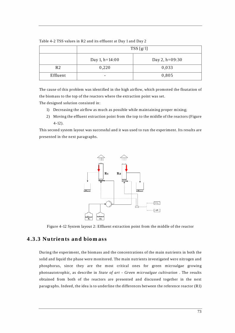
73
Table 4-2 TSS values in R2 and its effluent at Day 1 and Day 2
TSS [g/l]
Day 1, h=14:00 Day 2, h=09:30
R2 0,220 0,033
Effluent - 0,805
The cause of this problem was identified in the high airflow, which promoted the floatation of
the biomass to the top of the reactors where the extraction point was set.
The designed solution consisted in:
1) Decreasing the airflow as much as possible while maintaining proper mixing;
2) Moving the effluent extraction point from the top to the middle of the reactors (Figure
4-12).
This second system layout was successful and it was used to run the experiment. Its results are
presented in the next paragraphs.
Figure 4-12 System layout 2: Effluent extraction point from the middle of the reactor
4.3.3 Nutrients and biomass
During the experiment, the biomass and the concentrations of the main nutrients in both the
solid and liquid the phase were monitored. The main nutrients investigated were nitrogen and
phosphorus, since they are the most critical ones for green microalgae growing
photoautotrophic, as describe in State of art - Green microalgae cultivation . The results
obtained from both of the reactors are presented and discussed together in the next
paragraphs. Indeed, the idea is to underline the differences between the reference reactor (R1)
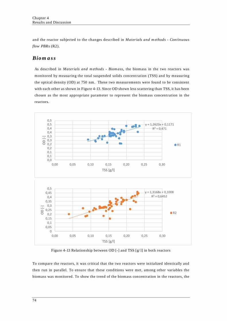
Chapter 4 Results and Discussion
74
and the reactor subjected to the changes described in Materials and methods - Continuous
flow PBRs (R2).
Biomass
As described in Materials and methods - Biomass, the biomass in the two reactors was
monitored by measuring the total suspended solids concentration (TSS) and by measuring
the optical density (OD) at 750 nm. These two measurements were found to be consistent
with each other as shown in Figure 4-13. Since OD shown less scattering than TSS, it has been
chosen as the most appropriate parameter to represent the biomass concentration in the
reactors.
Figure 4-13 Relationship between OD [-] and TSS [g/l] in both reactors
To compare the reactors, it was critical that the two reactors were initialized identically and
then run in parallel. To ensure that these conditions were met, among other variables the
biomass was monitored. To show the trend of the biomass concentration in the reactors, the
y = 1,2623x + 0,1171R² = 0,471
0,00,10,10,20,20,30,30,40,40,50,5
0,00 0,05 0,10 0,15 0,20 0,25 0,30
OD
[-]
TSS [g/l]
R1
y = 1,3168x + 0,1008R² = 0,6452
00,05
0,10,15
0,20,25
0,30,35
0,40,45
0,5
0,00 0,05 0,10 0,15 0,20 0,25 0,30
OD
[-]
TSS [g/l]
R2

75
measurements of OD along the experiment in both reactors are reported in Figure 4-14.
Despite the biomass changes in the reactors along the experiment, the two reactors were
running in parallel in period 1, when they were subjected to the same conditions (average
difference around 0,01). A slight gap was manifested during period 2 (average difference 0,05).
In particular, R2, under limited nitrogen supply due to the decreasing of N-to-P ratio from 17
molN/molP to 10 molN/molP, showed a lower level of biomass. Despite this, as soon as R2
was subjected again to the same conditions of R1 in period 3, its biomass went back to the same
level of R1 after circa 5 days.
Figure 4-14 OD along the experiment in both reactors
Two conclusions can be draw from the above analysis:
1) Green microalgae have shown the capacity to survive a period of limited nitrogen
supply and to go back to the previous equilibrium, when subjected to the same
conditions. This aspect may be essential, not only in a WWTP, where the input
conditions can easily vary, but also and especially in the TRENS system, where as
described in Background and Motivations - PBR, the influent to the PBRs regularly
suffers of drops in the N-to-P ratio.
2) It seems that a limited supply of nitrogen has only slight consequences on the
production of biomass. Anyhow, this aspect should be considered especially when the
biomass produced in the PBRs is intended to be harvested for the production of
secondary products, for instance biofuel.
Nitrogen
In the PBRs the nitrogen is situated in both the liquid phase and solid phase, i.e. as storage in
the green microalgae cells. In the liquid phase, it is present in form of NH4+, NO3- and NO2-.
0
0,1
0,2
0,3
0,4
0,5
0,0 5,0 10,0 15,0 20,0 25,0 30,0 35,0 40,0 45,0
[-]
[day]
OD
R1
R2
PERIOD 2 PERIOD 3PERIOD 1
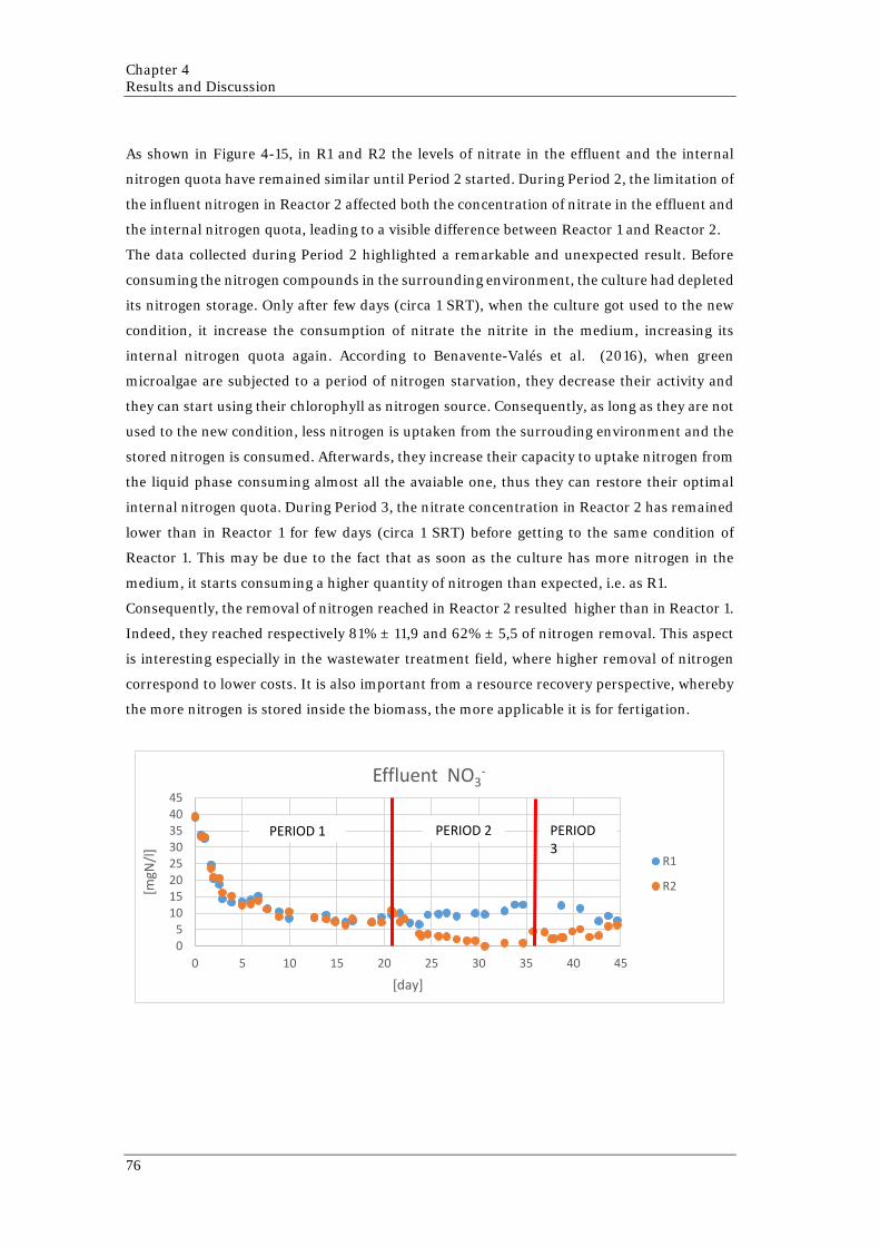
Chapter 4 Results and Discussion
76
As shown in Figure 4-15, in R1 and R2 the levels of nitrate in the effluent and the internal
nitrogen quota have remained similar until Period 2 started. During Period 2, the limitation of
the influent nitrogen in Reactor 2 affected both the concentration of nitrate in the effluent and
the internal nitrogen quota, leading to a visible difference between Reactor 1 and Reactor 2.
The data collected during Period 2 highlighted a remarkable and unexpected result. Before
consuming the nitrogen compounds in the surrounding environment, the culture had depleted
its nitrogen storage. Only after few days (circa 1 SRT), when the culture got used to the new
condition, it increase the consumption of nitrate the nitrite in the medium, increasing its
internal nitrogen quota again. According to Benavente-Valés et al. (2016), when green
microalgae are subjected to a period of nitrogen starvation, they decrease their activity and
they can start using their chlorophyll as nitrogen source. Consequently, as long as they are not
used to the new condition, less nitrogen is uptaken from the surrouding environment and the
stored nitrogen is consumed. Afterwards, they increase their capacity to uptake nitrogen from
the liquid phase consuming almost all the avaiable one, thus they can restore their optimal
internal nitrogen quota. During Period 3, the nitrate concentration in Reactor 2 has remained
lower than in Reactor 1 for few days (circa 1 SRT) before getting to the same condition of
Reactor 1. This may be due to the fact that as soon as the culture has more nitrogen in the
medium, it starts consuming a higher quantity of nitrogen than expected, i.e. as R1.
Consequently, the removal of nitrogen reached in Reactor 2 resulted higher than in Reactor 1.
Indeed, they reached respectively 81% ± 11,9 and 62% ± 5,5 of nitrogen removal. This aspect
is interesting especially in the wastewater treatment field, where higher removal of nitrogen
correspond to lower costs. It is also important from a resource recovery perspective, whereby
the more nitrogen is stored inside the biomass, the more applicable it is for fertigation.
05
1015202530354045
0 5 10 15 20 25 30 35 40 45
[mgN
/l]
[day]
Effluent NO3-
R1
R2
PERIOD 2 PERIOD 3
PERIOD 1

77
0
1
2
3
4
5
0 5 10 15 20 25 30 35 40 45
[mgN
/]
[day]
Effluent NO2
R1
R2
PERIOD 1 PERIOD2
PERIOD3
0
5
10
15
20
25
30
0 5 10 15 20 25 30 35 40 45
[mgN
/l]
[day]
Internal N quota
R1
R2
PERIOD 1 PERIOD 2 PERIOD 3
0,00
0,02
0,04
0,06
0,08
0,10
0,12
0,14
0 5 10 15 20 25 30 35 40 45
[mgN
/mgC
OD]
[day]
Internal N quota normalized to the biomass
R1
R2
PERIOD 1 PERIOD 2 PERIOD 3

Chapter 4 Results and Discussion
78
Figure 4-15 Nitrogen concentration in the liquid phase and in the cells in both reactors along the experiment
Mass balance
The mass balance of the experimental data was checked and a consistent gap was
found between the influent nitrogen and the effluent nitrogen.
The most likely cause may be a poor measurement accuracy. Indeed, first of all a
minimum of uncertainty in the experimental data has to be always considered.
Secondly, in this case, some concerns have been raised regarding the measurement of
the total nitrogen (TN). Indeed, the actual capacity of the method of being able to
extract the nitrogen from the green microalgae cells was never ascertained. Since in
literature it is reported that is in general difficult to extract proteins and lipids from
the green microalgae cells, it could be that this method has the same issues towards
components rich in nitrogen.
Figure 4-16 Nitrogen mass balance along the experiment for both reactors
0
20
40
60
0,0 2,6 6,7 13,9 19,7 24,6 30,6 40,7
[mgN
/l]
[day]
R1
Effluent soluble inorganic nitrogen Internal Nitrogen Influent Nitrogen
0
20
40
60
80
0,0 2,6 6,7 14,8 20,8 25,7 30,6 36,7 43,7 49,7
[mgN
/l]
[day]
R2
Effluent soluble inorganic nitrogen Internal Nitrogen Influent nitrogen
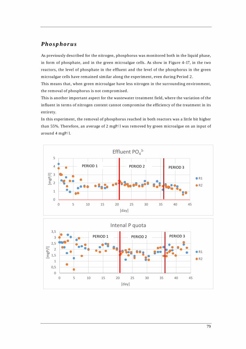
79
Phosphorus
As previously described for the nitrogen, phosphorus was monitored both in the liquid phase,
in form of phosphate, and in the green microalgae cells. As show in Figure 4-17, in the two
reactors, the level of phosphate in the effluent and the level of the phosphorus in the green
microalgae cells have remained similar along the experiment, even during Period 2.
This means that, when green microalgae have less nitrogen in the surrounding environment,
the removal of phosphorus is not compromised.
This is another important aspect for the wastewater treatment field, where the variation of the
influent in terms of nitrogen content cannot compromise the efficiency of the treatment in its
entirety.
In this experiment, the removal of phosphorus reached in both reactors was a little bit higher
than 55%. Therefore, an average of 2 mgP/l was removed by green microalgae on an input of
around 4 mgP/l.
0
1
2
3
4
5
0 5 10 15 20 25 30 35 40 45
[mgP
/l]
[day]
Effluent PO43-
R1
R2
PERIOD 1 PERIOD 2 PERIOD 3
0
0,5
1
1,5
2
2,5
3
3,5
0 5 10 15 20 25 30 35 40 45
[mgP
/l]
[day]
Intenal P quota
R1
R2
PERIOD 1 PERIOD 2 PERIOD 3

Chapter 4 Results and Discussion
80
Figure 4-17 Phosphorus concentration in the liquid phase and in the cells in both reactors
along the experiment
Mass balance
Differently from the nitrogen case, the overall mass balance for the phosphorus was found to
be respected. The error is around 4,3% for both reactors and it is acceptable considering the
possible errors occurring during sampling and measurement.
0,000
0,005
0,010
0,015
0,020
0,025
0,030
0,035
0 5 10 15 20 25 30 35 40 45
[mgP
/mgC
OD]
[day]
Internal P quota normalized to the biomass
R1
R2
PERIOD 1 PERIOD 2PERIOD 3
0
2
4
6
8
0 1 2 3 5 7 9 14 16 19 21 23 25 27 29 31 34 36 38 41 44
[mgP
/l]
[day]
R1
Effluent Phosphate Internal Phosphorus Influent Phosphate

81
Figure 4-18 Phosphorus mass balance along the experiment for both reactors
4.4 Green microalgae culture history and the
nutrients uptake and storage
One of the aim of this work was to verify the existence of a link between the history of the
culture and its uptake and storage of nutrients. With this purpose, two batches were run as
described in Materials and methods - 1.2 L s. The cultures used in these experiments were
exposed to the same N-to-P ratio during the experiments, but they had two different histories:
one was used to grow in a medium with 17 N-to-P ratio ( 17-17 Batch), the other was used to
grow in a medium with 10 N-to-P ratio (10-17 Batch). To assess the differences in the nutrients
uptake and storage in the two cases, two parameters sets where estimated, one for each case,
as described in the following paragraphs.
4.4.1 ASM-A MODEL: Parameters estimations
The method Latin Hypercube Sampling based Simplex (LHSS) was used to estimate the kinetic
parameters and to assess their identifiability. It is described in details in Materials and
methods - Parameters estimation, but more informations can be found in Wágner et al.(2016).
17-17 Batch
Before starting the parameters estimation, a simulation of this experiment, using the
parameters set given by Wágner et al. (2016), was run to verify the necessity of the parameters
estimation itself. As shown in Figure 4-19, the prediction of the model in this case is inaccurate,
especially regarding the growth of the biomass, which in turn influences the other variables.
The sum of RMSNE resulted equal to 3,60.
0
2
4
6
8
0 1 2 3 5 7 9 13 15 17 20 21 23 24 25 27 29 31 34 36 37 38 39 41 43 45
[mgP
/l]
[day]
R2
Effluent Phosphate Internal Phosphorus Influent Phosphorus
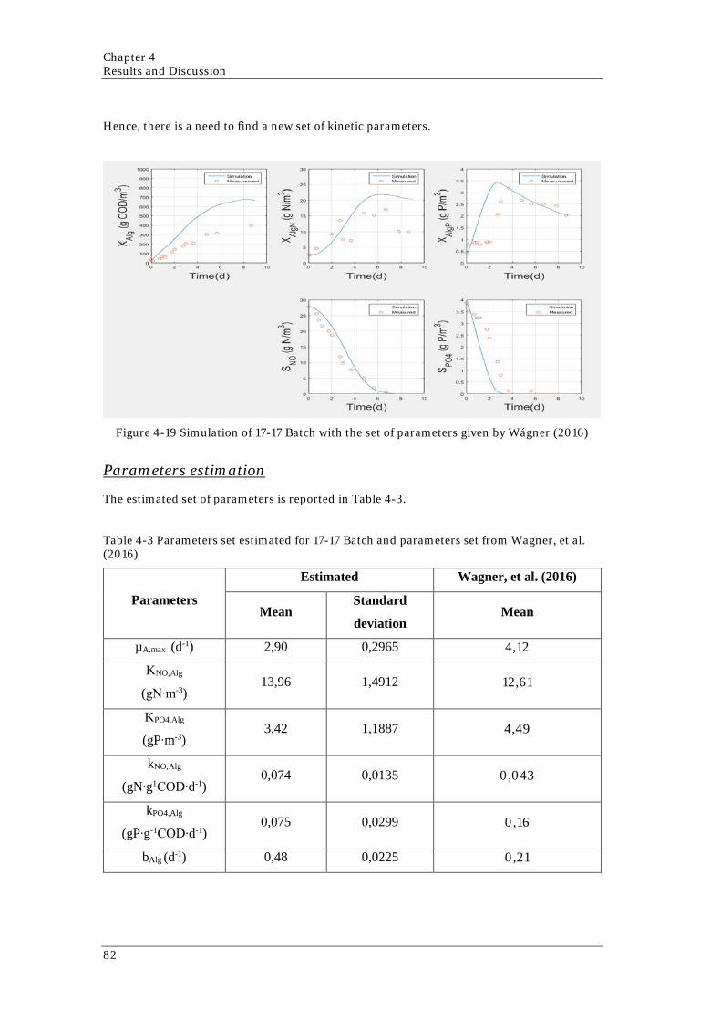
Chapter 4 Results and Discussion
82
Hence, there is a need to find a new set of kinetic parameters.
Figure 4-19 Simulation of 17-17 Batch with the set of parameters given by Wágner (2016)
Parameters estimation
The estimated set of parameters is reported in Table 4-3.
Table 4-3 Parameters set estimated for 17-17 Batch and parameters set from Wagner, et al. (2016)
Parameters
Estimated Wagner, et al. (2016)
Mean Standard
deviation Mean
µA,max (d-1) 2,90 0,2965 4,12
KNO,Alg
(gN∙m-3) 13,96 1,4912 12,61
KPO4,Alg
(gP∙m-3) 3,42 1,1887 4,49
kNO,Alg
(gN∙g1COD∙d-1) 0,074 0,0135 0,043
kPO4,Alg
(gP∙g-1COD∙d-1) 0,075 0,0299 0,16
bAlg (d-1) 0,48 0,0225 0,21

83
The prediction of the model using the new kinetic parameters is shown in Figure 4-20. If these
results are compared to the ones shown in Figure 4-19, which were obtained using the
parameters set proposed in Wágner et al. (2016), a good improvement can be seen especially
regarding the prediction of algal biomass, internal phosphorus quota and phosphate.
Moreover, the improvement is quantifiable comparing the sum of RMSNE of the simulations.
Indeed, it is reduced from 3,60 to 2,30 giving a Janus coefficient of 0,64.
Figure 4-20 Simulation of 17-17 Batch with the estimated parameters set
Identifiability
In accordance with what is described in Materials and methods - Identifiability analysis, the
identifiability of the parameters was assessed.
The standard deviations reported in Table 4-3 are relatively low considering the respective
parameter values and the parameters distribution represented in the histograms in Table 4-4
can be considered narrow. Nevertheless, based on the correlation matrix (Table 4-4) some
parameters (µA,max and kNO,Alg; µA,max and kPO4,Alg; KPO4,Alg and kPO4,Alg) seems to be correlated.

Chapter 4 Results and Discussion
84
Table 4-4 Parameters distribution and correlation matrix
To verify the actual presence of a correlation between these parameters, the impact of the
parameters variability on the model output was assessed. To this aim, the simulation results
using the values of the parameters on the boundaries given by their standard deviations were
compared with the simulation results using the mean values of the parameters. The
parameters chosen for this purpose were µA,max and kPO4,Alg. To compare the results, Janus
coefficients were calculated and, as reported in Table 4-5, a low variation in the model output
was found in each case, because the Janus coefficients were ~ 1. Therefore, the parameters are
considered identifiable.
µA,max
(d-1)
KNO,Alg
(gN∙m-3)
KPO4,Alg
(gP∙m-3)
kNO,Alg
(gN∙g1COD∙d-1)
kPO4,Alg
(gP∙g-1COD∙d-1)
bAlg
(d-1)
µA,max
(d-1) 1
KNO,Alg
(gN∙m-3) 0,1263 1
KPO4,Alg
(gP∙m-3) -0,2424 -0,2906 1
kNO,Alg
(gN∙g1COD∙d-1) -0,7337 0,4247 -0,0396 1
kPO4,Alg
(gP∙g-1COD∙d-1) -0,6719 -0,3477 0,7728 0,3794 1
bAlg
(d-1) -0,0712 0,089 0,3215 0,3102 0,2971 1

85
Table 4-5 Janus coefficients used to assess the impact of the parameters variability on the model output
µA,max + sd µA,max - sd kPO4,Alg + sd kPO4,Alg - sd
Janus
coefficient 1,1680 1,0554 1,0825 1,0647
4.4.2 10-17 Batch
The procedure used for Batch 17-17 was applied verbatim to Batch 10-17.
To assess the need of the parameters estimation, a simulation using the parameters set given
by Wágner (2016) was run. From Figure 4-21, it can be seen that the prediction of the model
fails in particular regarding the biomass and the phosphate. Therefore, a new set of kinetic
parameters needs to be estimated. The sum of RMSNE resulted equal to 2,96.
Figure 4-21 Simulation 10-17 Batch with parameters set given by Wágner (2016)

Chapter 4 Results and Discussion
86
Parameters estimation
The parameters set estimated is reported in Table 4-6.
Table 4-6 Parameters set estimated for 10-17 Batch
Parameters
Estimated Wagner, et al. (2016)
Mean Standard
deviation Mean
µA,max (d-1) 3,18 0,4365 4,12
KNO,Alg
(gN∙m-3) 12,49 2,7716 12,61
KPO4,Alg
(gP∙m-3) 4,70 0,4770 4,49
kNO,Alg
(gN∙g1COD∙d-1) 0,074 0,0144 0,043
kPO4,Alg
(gP∙g-1COD∙d-1) 0,042 0,0113 0,16
bAlg (d-1) 0,48 0,0187 0,21
The prediction of the model using the new kinetic parameters is shown in Figure 4-22.
Comparing these results with the ones shown in Figure 4-21, which were obtained using the
parameters set proposed in Wágner (2016), a good improvement can be seen especially
regarding the prediction of algal biomass and phosphate. Moreover, the improvement is
observable comparing the sum of RMSNE of the simulations. Indeed, it is changed from 2,96
to 1,54 giving a Janus coefficient of 0,52.
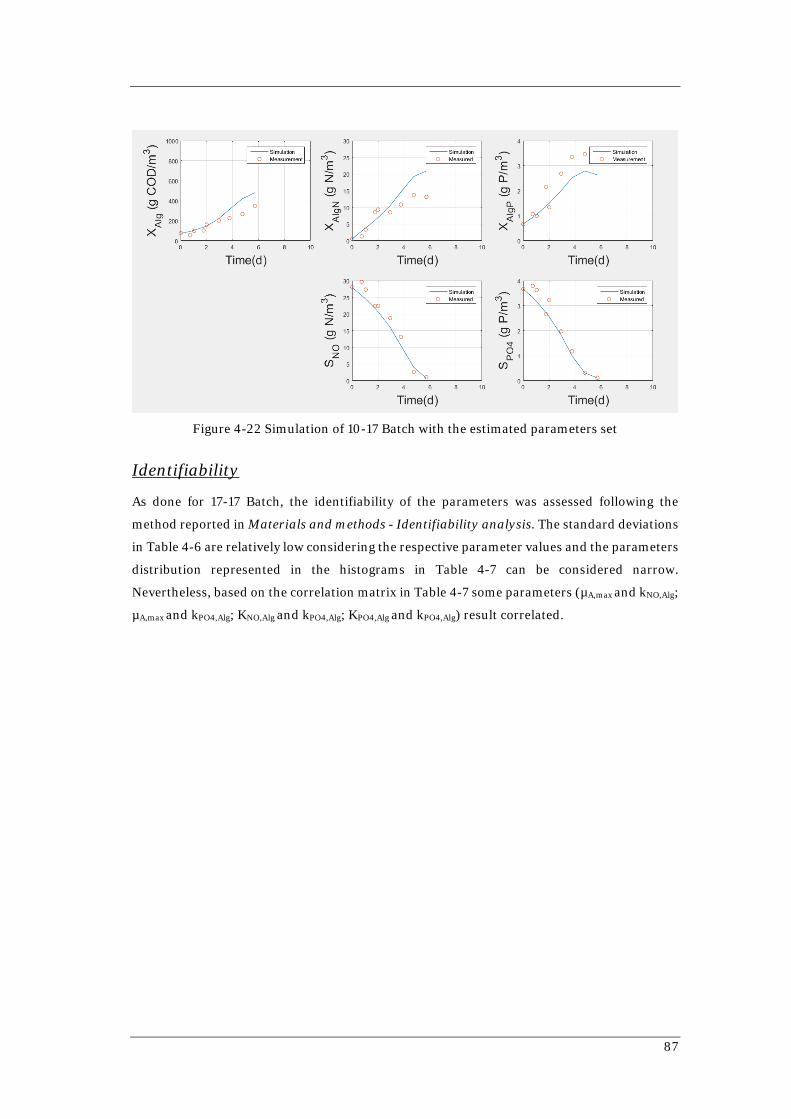
87
Figure 4-22 Simulation of 10-17 Batch with the estimated parameters set
Identifiability
As done for 17-17 Batch, the identifiability of the parameters was assessed following the
method reported in Materials and methods - Identifiability analysis. The standard deviations
in Table 4-6 are relatively low considering the respective parameter values and the parameters
distribution represented in the histograms in Table 4-7 can be considered narrow.
Nevertheless, based on the correlation matrix in Table 4-7 some parameters (µA,max and kNO,Alg;
µA,max and kPO4,Alg; KNO,Alg and kPO4,Alg; KPO4,Alg and kPO4,Alg) result correlated.

Chapter 4 Results and Discussion
88
Table 4-7 Parameters distribution and correlation matrix
Equally to what was done for 17-17 Batch, to verify the actual presence of a correlation between
these parameters, the impact of the parameters variability on the model output was assessed.
The parameters chosen for this purpose were µA,max , kPO4,Alg and KNO,Alg.
The Janus coefficients calculated (Table 4-8) were around 1, therefore, a low variation in the
model output was found in each case. Consequently, the parameters are considered
identifiable.
µA,max
(d-1)
KNO,Alg
(gN∙m-3)
KPO4,Alg
(gP∙m-3)
kNO,Alg
(gN∙g1COD∙d-1)
kPO4,Alg
(gP∙g-1COD∙d-1)
bAlg
(d-1)
µA,max
(d-1) 1 0,1439 -0,136 -0,6659 -0,7657 0,2355
KNO,Alg
(gN∙m-3) 0,1439 1 -0,189 0,5916 -0,3035 0,3201
KPO4,Alg
(gP∙m-3) -0,136 -0,1892 1 -0,1311 0,5432 0,0651
kNO,Alg
(gN∙g1COD∙d-1) -0,666 0,5916 -0,131 1 0,3536 0,1552
kPO4,Alg
(gP∙g-1COD∙d-1) -0,766 -0,3035 0,543 0,3536 1 0,0171
bAlg
(d-1) 0,2355 0,3201 0,065 0,1552 0,0171 1
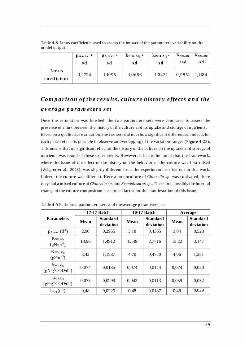
89
Table 4-8 Janus coefficients used to assess the impact of the parameters variability on the model output
µA,max +
sd
µA,max -
sd
kPO4,Alg +
sd
kPO4,Alg -
sd
KNO,Alg
+sd KNO,Alg
-sd
Janus
coefficient 1,2724 1,1095 1,0686 1,0421 0,9851 1,1184
Comparison of the results, culture history effects and the
average parameters set
Once the estimation was finished, the two parameters sets were compared to assess the
presence of a link between the history of the culture and its uptake and storage of nutrients.
Based on a qualitative evaluation, the two sets did not show significant differences. Indeed, for
each parameter it is possible to observe an overlapping of the variation ranges (Figure 4-23).
This means that no significant effect of the history of the culture on the uptake and storage of
nutrients was found in these experiments. However, it has to be noted that the framework,
where the issue of the effect of the history on the behavior of the culture was first raised
(Wágner et al., 2016), was slightly different from the experiments carried out in this work.
Indeed, the culture was different. Here a monoculture of Chlorella sp. was cultivated, there
they had a mixed culture of Chlorella sp. and Scenedesmus sp.. Therefore, possibly the internal
change of the culture composition is a crucial factor for the manifestation of this issue.
Table 4-9 Estimated parameters sets and the average parameters set
Parameters 17-17 Batch 10-17 Batch Average
Mean Standard deviation Mean
Standard deviation Mean
Standard deviation
µA,max (d-1) 2,90 0,2965 3,18 0,4365 3,04 0,528 KNO,Alg
(gN∙m-3) 13,96 1,4912 12,49 2,7716 13,22 3,147
KPO4,Alg
(gP∙m-3) 3,42 1,1887 4,70 0,4770 4,06 1,281
kNO,Alg
(gN∙g1COD∙d-1) 0,074 0,0135 0,074 0,0144 0,074 0,020
kPO4,Alg
(gP∙g-1COD∙d-1) 0,075 0,0299 0,042 0,0113 0,059 0,032
bAlg (d-1) 0,48 0,0225 0,48 0,0187 0,48 0,029

Chapter 4 Results and Discussion
90
Considering the relatively low discrepancy between the two sets of parameters estimated, it
seemed appropriate to test the operation of the model using an average parameters set, that
could potentially fit for both cases. The average parameters set was easily calculated doing an
average of the estimated two parameters sets, while the standard deviation were calculating
using Equation 4-2. (Table 4-9).
𝑆𝑆𝑔𝑔𝐷𝐷𝐴𝐴𝐴𝐴 = �𝑆𝑆𝑔𝑔𝐷𝐷17−172 + 𝑆𝑆𝑔𝑔𝐷𝐷10−172
Equation 4-2 Standard deviation for average parameter set calculation
Where:
SDAV= Standard deviation of parameter x of the average parameter set
SDx17-17= Standard deviation of parameter x of the 17-17 Batch parameter set
SDx10-17= Standard deviation of parameter x of the 10-17 Batch parameter set
Figure 4-23 Comparison of the variation ranges of the three parameters set involved
To assess the feasibility of the use of the average parameters set, simulations of 17-17 Batch
and of 10-17 Batch were run using this new set. Once again, the Janus coefficient was used to
2,9
3,2
3,0
2,0 3,0 4,0 1/d
µmaxBatch 17-17
Batch 10-17
Average
14,0
12,5
13,2
9,0 14,0 19,0 gN/m3
KNO,AlgBatch 17-17
Batch 10-17
Average
3,4
4,7
4,1
1,5 3,5 5,5 7,5 gP/m3
KPO4,AlgBatch 17-17
Batch 10-17
Average
0,0745
0,0745
0,0745
0,050 0,075 0,100gN/(gCOD∙d)
kNO,AlgBatch 17-17Batch 10-17Average
0,076
0,042
0,059
0,02 0,05 0,07 0,10 0,12gP/(gCOD∙d)
kPO4,AlgBatch 17-17
Batch 10-17
Average
0,480
0,4830,481
0,440 0,460 0,480 0,500 0,520 1/d
bAlg
Batch 17-17
Batch 10-17
Average

91
compare the results of these simulations with the simulations previously performed with the
parameters sets estimated in this chapter.
Table 4-10 Janus coefficients used to compare the simulations done using the average parameters set and the estimated ones for both 17-17 batch and 10-17 Batch
17-17 Batch 10-17 Batch
Janus coefficient 0,9983 1,0760
From the obtained results (Table 4-10), the average parameters set seems to be applicable in
both cases, without compromising the model prediction.
To further verify the accuracy of the model using the average parameters set, Monte Carlo
simulations were performed (Figure 4-24 and Figure 4-25). The outcomes shown again the
applicability of the average parameters set in both cases.
Figure 4-24 Monte Carlo simulation for 17-17 Batch with average parameters set
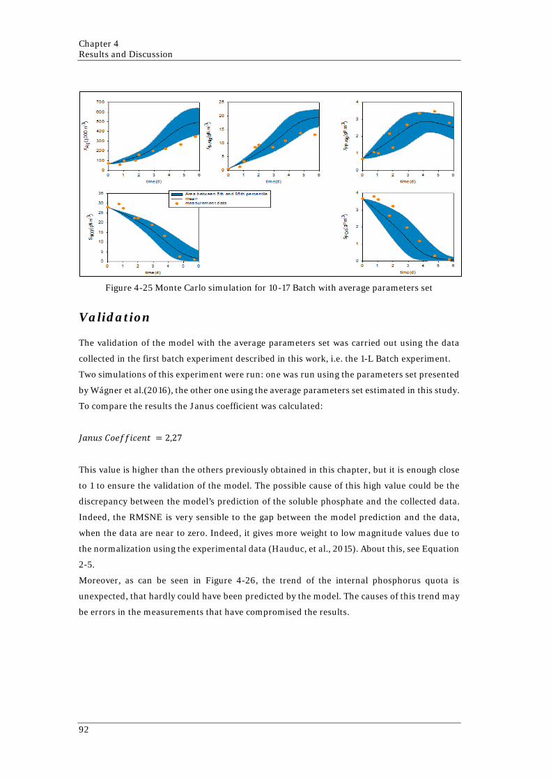
Chapter 4 Results and Discussion
92
Figure 4-25 Monte Carlo simulation for 10-17 Batch with average parameters set
Validation
The validation of the model with the average parameters set was carried out using the data
collected in the first batch experiment described in this work, i.e. the 1-L Batch experiment.
Two simulations of this experiment were run: one was run using the parameters set presented
by Wágner et al.(2016), the other one using the average parameters set estimated in this study.
To compare the results the Janus coefficient was calculated:
𝐽𝐽𝑝𝑝𝑛𝑛𝑛𝑛𝑠𝑠 𝐶𝐶𝑜𝑜𝑒𝑒𝑜𝑜𝑜𝑜𝐿𝐿𝑝𝑝𝑒𝑒𝑛𝑛𝑡𝑡 = 2,27
This value is higher than the others previously obtained in this chapter, but it is enough close
to 1 to ensure the validation of the model. The possible cause of this high value could be the
discrepancy between the model’s prediction of the soluble phosphate and the collected data.
Indeed, the RMSNE is very sensible to the gap between the model prediction and the data,
when the data are near to zero. Indeed, it gives more weight to low magnitude values due to
the normalization using the experimental data (Hauduc, et al., 2015). About this, see Equation
2-5.
Moreover, as can be seen in Figure 4-26, the trend of the internal phosphorus quota is
unexpected, that hardly could have been predicted by the model. The causes of this trend may
be errors in the measurements that have compromised the results.

93
Figure 4-26 Simulation of 1-L Batch using the average parameter set
To further consolidate the validation a Monte Carlo simulations were performed. As can be
seen in Figure 4-27, where the results are shown, the observations often either fall out from
the area between the 5th and the 95th percentile or on the boundaries of that area. Anyhow, this
does not imply the failure of the validation. Indeed, it has to be noticed that for the experiment
(1-L Bacth) the input light intensity to the reactor was not monitored, therefore an average
light intensity in the reactor was theoretically calculated and assumed constant along the
experiment. The effects of this assumption may have caused the underestimation of the
biomass production (XAlg) and in turn the underestimation of the phosphorus uptake (SPO4)
and storage (XPPAlg).
Figure 4-27 Monte Carlo simulation for 1-L Batch with average parameters set

Chapter 4 Results and Discussion
94
Application of the new parameters set to the continuous
PBRs case
The sets of the kinetic parameters estimated in the previous paragraphs were applied with
different combinations to simulate the continuous PBRs experiment.
For Reactor 1, which had for the entire experiment an influent N-to-P ratio of 17 molN/molP,
the simulations were run using the parameters set from 17-17 Batch and the average parameter
set. Instead, for Reactor 2, which had three different influent N-to-P ratio as described in
Materials and methods - Continuous flow PBRs, different parameters sets within the same
simulation were used. One simulation was run using the parameters set from 17-17 Batch for
Period 1 and Period 2 and the parameters set from 10-17 Batch for Period 3. The other
simulation was run using the average parameters set.
The results are reported respectively in Figure 4-28 and in Figure 4-29. In those figures, the
results of the simulations run using the parameters set from Wágner et al.(2016) is reported
as well to show the improvements obtained in the model prediction using the new parameters
sets.
In both cases, it is clear that a significant improvement is achieved using the new parameters
sets instead of the parameters set from Wágner et al. (2016). Moreover, the average parameters
set has proven to be the best one for the predictions. These results are interesting, because it
means that, once an average parameters set is defined, it is possible to simulate with a good
accuracy the trends in the PBR whatever are the conditions which the green microalgae are
subjected to.
Despite the good results obtained in both cases, the prediction of the internal nitrogen quota
fails at the beginning of Period 2 in R2 when the N-to-P ratio decreased to 10 molN/molP. The
simulation does not follow the data (green square) due to the unexpected behavior of the
culture in the first days of nitrogen starvation described in Results and Discussion -
Continuous flow PBRs - Nitrogen, which is not modeled in the ASM-A model.

95
REACTOR 1
Simulation with the parameters set from Wágner (2016) – RMSNE = 11,97
Simulation with the parameters set from 17-17 Batch - RMSNE = 9,13
Simulation with the average parameters set - RMSNE = 8,74
Figure 4-28 Simulations of Reactor 1 with different parameters sets

Chapter 4 Results and Discussion
96
REACTOR 2
Simulation with the parameters set from Wágner (2016) – RMSNE = 27,32
Simulation with:
- Period 1 and period 2: the parameters set from 17-17 Batch
- Period 3: the parameters set from 10-17 Batch RMSNE = 23,32
Simulation with the average parameters set - RMSNE = 22,6
Figure 4-29 Simulations of Reactor 2 with different parameters set

97
4.5 Images analysis
4.5.1 Development of a new images analysis method
Two cultures were used to develop a new automated image analysis method aimed to quantify
the microbial community. The two cultures had different composition:
1. A mixed green microalgae culture containing mostly Chlorella sp. and Scenedesmus
sp. ;
2. A monoculture containing uniquely Chlorella sp..
Figure 4-30 On the left a picture of Chlorella sp., on the right a picture of Scenedesmus sp.
The different green microalgae types were distinguished according to their morphology, i.e.
Chlorella sp. (shape: round and small individual cells) and Scenedesmus sp. (shape: elongated
cells grown in four-cell colonies). As reported in Materials and methods - Microscopy and
image analysis, images were taken using a Motic AE31 microscope with a magnification of
20x. 60 images were obtained for the mixed culture, two sets of 30 images were instead
obtained for the monoculture.
To distinguish between the genera, morphological descriptors (area, diameter or the aspect
ratio) of each type were automatically acquired using the image analysis software Image pro
plus 7 3D suite (USA). The morphological descriptors are case specific. Same species in
different culture may need different morphological descriptors. Therefore, it is suggested to
calibrate them every time a new culture is studied. Thanks to this software, the number of
cells for each group of green microalgae were easily counted.
In both cases the minimum image number required to yield a representative average cells
count was assessed. The minimum number was found as the one for which an additional image
gives a margin of improvement of less than 5%.
As shown in Figure 4-31 and Figure 4-32, different results were found for the mixed culture
and the monoculture. The minimum number of images necessary to quantify the number of
cells in a mixed culture was found to be 17. Instead, the minimum number of images necessary
to quantifiy the number of cells in a monoculture was 10.

Chapter 4 Results and Discussion
98
Figure 4-31 Cumulative average cells count for mixed culture of Chlorella sp. and
Scenedesmus sp.
Figure 4-32 Cumulative average cells count for monoculture of Chlorella sp.
4.5.2 Application of the new images analysis method to two
continuous flow PBRs
The new images analysis method described in the previous paragraph was applied on the
main experiment carried out in this work, i.e. the 2 continuous PBRs.
Indeed, one of the goals of this experiment was to assess the effects of the variation of the input
N-to-P ratio on the green microalgae culture in terms of composition and unexpected
contaminations.
Approximately every second day 10 images were taken for the PBRs and they were analyzed as
previously explained.
02468
10121416
0 10 20 30 40 50 60
Cum
ulat
ive
ave
rage
cel
ls co
unt
[-]
Number of images [-]
Chlorella sp.
Scenedesmus
- Minimum number of images
0,0
50,0
100,0
150,0
200,0
250,0
300,0
0 5 10 15 20 25 30
Cum
ulat
ive
ave
rage
cells
co
unt [
-]
Number of images [-]
SET_1
SET_2
- Minimum number of images

99
Only Chlorella sp. was found in the reactors for about 45 days, i.e. for the entire length of the
experiment. Therefore, the culture did not change and no contamination occurred. This
probably means that a healthy culture is strong enough to compete against other potential
microorganisms that enter into the PBR through the wastewater, even when it is subject to
variation in the N-to-P ratio. This is important when we consider cultivation of microalgae in
open systems on wastewater, where culture stability is considered to be an issue.
Figure 4-33 Number of Chlorella sp. cells along the experiment in R1 and R2
As already highlighted by other parameters for the measurement of the biomass, i.e. TSS and
OD, are no significant changes ae observed in the biomass when the N-to-P ratio is changed.
Indeed, as shown in Figure 4-33, the number of cells in R1 e R2 remained almost equal during
the experiment.
The reliability of the measurement was assessed comparing the OD measurement with the
relative number of Chlorella sp. cells found through the new method (Figure 4-34). Although
in the plot some scattering is shown, the two measurements can be considered correlated.
Figure 4-34 OD vs Number of Chlorella sp. cells to assess the reliability of the measurement
0
50
100
150
200
250
300
0 5 10 15 20 25 30 35 40 45
Num
ber o
f Chl
orel
la sp
. cel
ls [-]
[days]
R1
R2
- Changed N-to-P ratio in R2 influent
00,05
0,10,15
0,20,25
0,30,35
0,40,45
0,5
0 50 100 150 200 250 300
OD
[-]
Number of Chlorella sp. cells [-]


100
CONCLUSION
During this study, experiments on the cultivation of green microalgae in wastewater were
conducted.
1. Starting from the problems pointed out in Valverde-Pérez et al. (2015) about the
variation of the medium composition in input to the PBRs in the TRENS, the
consequensis on microalgae culture of changings in the influent N-to-P ratio were
investigated. The results obtained revealed that the culture stability was not affected.
Indeed, the culture composition was maintained and no contaminations occurred.
Moreover, microalgae were able to keep a certain level of biomass along the
experiment, showing the ability to reestablish it when subjected to limited variations
in the N-to-P ratio. Regarding the efficiency of nutrients removal from the wastewater,
it was found that the overall nitrogen removal was enhanced when microalgae were
subjected to a period of nitrogen limitation. Instead, no effects on the overall
phosphorus removal were observed. Finally, the variability of the N-to-P ratio in input
to the PBRs reported by Valverde-Pérez et al. (2015) might not compromise the
operation of the system.
2. The effects of the culture history on the on the kinetics of microalgae processes were
investigated and from this study no relevant influence was found. From the kinetic
parameters sets estimated to assess the effects of the culture history, it was possible to
obtain an average parameters set, that used in the ASM-A model, gives the best results
for prediction of the two continuous flow PBRs run in this work. Therefore, estimating
an average parameters set, it may be possible to model a continuous flow PBRs, even
if it is subjected to an unstable influent composition in term of nutrients content.
3. The new automated image analysis method developed during this work was tested on
the experiments conducted and it was found to be able to identify different microalgae
species and to quantify them.


101
RECOMMENDATIONS
Based on the work done and the results obtain, few recommendations are here suggested:
1. Further investigating the possibility to enhance the removal of nitrogen exposing the
green microalgae culture to cycle of nitrogen starvation in a continuous flow PBR;
2. Studying the effects on the green microalgae culture when it is exposed to phosphorus
limitation to assess the possibility to improve its removal as observed for nitrogen;
3. Improving the model prediction when the culture is subjected to nitrogen limitation.
4. Assessing the effects of culture history on the uptake and storage of N and P in case of
mixed culture;
5. Investigating the causes of the unexpected gap in the nitrogen mass balance found in
the continuous flow PBRs experiment;
6. Testing the new image analysis method on cultures with different microalgae species.


102
References
[1] Cai , T., Park , S. . Y. & Li, Y., 2013. Nutrient recovery from wastewater streams bymicroalgae: Status and prospects. Renewable and Sustainable Energy Reviews,Volume 19, pp. 360-369.
[2] Christensen, T. B. & Hauggaard-Nielsen, H., 2015. Circular Economy - A review ofthe concept and examples of emerging practices. Sitges, s.n.
[3] Abdel-Raouf, N., Al-Homaidan, A. & Ibraheem, I., 2012. Microalgae and wastewatertreatment. Saudi Journal of Biological Sciences, Volume 19, pp. 257-275.
[4] Ambrose, R., 2006. Wasp7 benthic algae-model theory and users guide. Athens,Georgia: USEPA, Office of research and development.
[5] Apples, L., Baeyens, J., Degrève, J. & Dewil , R., 2008. Principles and potential of theanaerobic digestion of waste-activated sludge. Progress in Energy and CombustionScience, Volume 34, pp. 755-781.
[6] Arbib, Z. et al., 2013. Photobiotreatment: Influece of nitrogen and phosphorus ratioin wastewater on growth kinetics of Scenedesmus Obliquus. International Journal ofPhytoremediation, Volume 15, pp. 774-788.
[7] Arbib, Z. et al., 2013. Photobiotreatment: Influence of Nitrogen and Phosphorus ratioin wastewater on growth kinetics of Scenedesmus Obliquus. International Journal ofPhytoremediation, Volume 15, pp. 774-788.
[8] Azov, Y., 1982. Effect of pH on Inorganic Carbon Uptake in Algal Cultures. Appliedand Enviromental Microbiology, 43(6), pp. 1300-1306.
[9] Azov, Y. & Goldman, J., 1982. Free ammonia inhibition of algal photosynthesis inintensive cultures. Applied and Environmental Microbiology, 43(4), pp. 735-739.
[10] Benavente-Valés, J. R. et al., 2016. Strategies to enhance the production ofphotosyntetic pigments and lipids in chlorophycae species. biotechnology Reports,Volume 10, pp. 117-125.
[11] Benson, B., Gutierrez-Wing, M. & Rusch, K., 2007. The development of a mechanisticmodel to investigate the impacts of the light dynamics on algal productivity in aHydraulically Integrated Serial Turbidostat Algal Reactor (HISTAR). In:s.l.:Aquacultural Engineering, pp. 198-211.
[12] Bernard, O., 2011. Hurdles and challenges for modelling and control of microalgae foCO2 mitigation and biofuel production. Journal of Process Control, Volume 21, pp.1378-1389.
103
[13] Beuckles, A., Smolders, E. & Muylaert, K., 2015. Nitrogen availability influences phosphorus removal in microalagae-based wastewater treatment. Water Research, Volume 77, pp. 98-106.
[14] Bezzera, R. et al., 2013. Fed-batch cultivation of Arthrospira platensis using carbon dioxide from alcoholic fermentation and urea as carbon and nitrogen sources. Bioenergy Research, pp. 1-8.
[15] Boussiba, S., 1989. Ammonia uptake in the alkalophilic cyanobacterium Spirulina platensis. Plant and Cell Physiology, 30(2), pp. 303-308.
[16] Boussiba, S. & Gibson, J., 1991. Ammonia translocation in cyanobacteria. FEMS Microbiology Letters, 88(1), pp. 1-14.
[17] Broekhuizen, N., Park, J., McBride, G. & Craggs, R., 2012. Modification, calibration and verification of the IWA River Water Quality Model to simulate a pilot-scale high rate algal pond. Water Research, Volume 46, pp. 2911-2926.
[18] Brown, L., 1981. World population growth, soil erosion, and food security.. Science, 214(4524), pp. 995-1002.
[19] Brussaard, C., Brookes, R., Noordeloos, A. & Riegman, R., 1998. Recovery of nitrogen-starved cultures of the diatom Ditylum brightwellii (Bacillariophyceae) upon nitrogen resupply. Journal of Experimental Marine Biology and Ecology, 227(2), pp. 237-250.
[20] Cai, T., Park, S. & Li, Y., 2013. Nutrient recovery from wastewater streamns by microalgae: status and prospects. Renewable Sustainable Energies Reviewa, Volume 19, pp. 360-369.
[21] Carballa, M., Regueiro, L. & Lema, J., 2015. Microbial management of anaerobic digestion: exploiting the microbiome-functionality nexus. Current Opinion in Biotechnlogy, Volume 33, pp. 103-111.
[22] Carey, R. O. & Migliaccio, K. W., 2009. Contribution of Wastewater Treatment Plant Effluents to Nutrient Dynamics in Aquatic System: A Review. Environmental Management, Volume 44, pp. 205-217.
[23] Chi, Z., O'Fallon, J. & Chen, S., 2011. Bicarbonate produced from carbon capture for algae culture. Trends in Biotechnology, 29(11), pp. 537-541.
[24] Chi, Z., Zheng, Y., Jiang, A. & Chen, S., 2011. Lipid production by culturing oleaginous yest and algae with wood waste and municipal wastewater un an integrated process. Applied Biochemestry and Biotechnology, Volume 165, pp. 442-453.
[25] Choi, H. J. & Lee, S. M., 2015. Effect of the N/P ratio on biomass productivity and nutrient removal from municipal wastewater. Bioprocess Biosystem Engineering, 38(4), pp. 761-766.
[26] Cohen, J. E., 1995. Population Growth and Earth's Human Carrying Capacity. Science, 269(5222), pp. 341-236.
[27] Colak, O. & Kaya, Z., 1988. A study on the possibilities of biological wastewater treatment using algae. Doga Biyolji Serisi, 12(1), pp. 18-29.
[28] CSS, 2015. U.S. Water Supply and Distribution Factsheet. s.l.:s.n.

References
104
[29] De la Noüe, J. & De Pauw, N., 1988. The potential of microalgal biotechnology. A review of production and uses of microalgae. Biotechnology Advances, Volume 6, pp. 725-770.
[30] De Mes, T., Stams, A., Reith, J. & Zeeman, G., 2003. Methane production by anaerobic digestion of wastewater and solid wastes. In: Bio-methane & Bio-hydrogen. s.l.:s.n., pp. 58-102.
[31] Decostere, B. et al., 2013. A combined respirometer-titrimeter for the determination of microalgae kinetics: experimental data collection and modelling. Chemical Engineering Journal, Volume 222, pp. 85-93.
[32] Doria, E. et al., 2012. Isolation and characterization of a Scenedesmus acutus strain to be used for bioremediation of urban wastewater. Applied Phycology, Volume 24, pp. 375-383.
[33] Droop, M., 1973. Some thoughts on nutrient limitation in algae. Journal of Phycology, 9(3), pp. 264-272.
[34] Dyhrman, S. & Ruttenberg, K., 2006. Presence and regulation of alkaline phosphatase activity in eukaryotic phytoplankton from the coastal ocean: Implications for dissolved organic phosphorus remineralization. Limnology and Oceanography, 51(3), pp. 1381-1390.
[35] Eixler, S., Karsten, U. & Selig, U., 2006. Phosphous storage in Chlorella Vulgaris (Trebouxiophycae, Chlorophyta) cells and its dependence on phosphate supply. Phycologia, 45(1), pp. 53-60.
[36] El-Sheek, M. M. & Rady, A. A., 1995. Effect of phosphorus starvation on growth, photosynthesis and some metabolic processess in the unicellular green algae Chlorella kessleri. Phyton, Volume 35, pp. 1139-1151.
[37] Evonne, P. & Tang, 1997. Polar cyanobacteria versus green algae for tertiary waster treatment in cool climates. Journal of Applied Phycology, Volume 9, pp. 371-381.
[38] Fachet, M., Flassig, R., Rinhko-Struckmann, L. & Sundmacher, K., 2014. A dynamic growth model of Dunaliella salina: Parameter identification and profile likelihood analysis.. Bioresource Technology, Volume 173, pp. 21-31.
[39] Fang, L. et al., 2015. Life cycle assessment as development and decision support tool for wastewater resource recovery technlogy. Waster Research, Volume 88, pp. 538-459.
[40] FAO, 2016. FAOSTAT. [Online] Available at: http://faostat3.fao.org/browse/E/EL/E [Consultato il giorno July 2016].
[41] Flores, E. & Herrero, A., 2005. Nitrogen assimilation and nitrogen control in cyanobacteria. Biochemical Society Transactions, 33(1), pp. 164-167.
[42] Flores, E., Herrero, A. & Miguel, G., 1987. Nitrite uptake and its regulation in the cyanobacterium Anacystis nidulans. Biochimica et Biophysica Acta (BBA), 896(1), pp. 103-108.

105
[43] Fuggi, A., 1993. Uptake and assimilation of nitrite in the acidophilic red alga Cyanidium caldarium Geitler. New Phytologist, 125(2), pp. 351-360.
[44] Geider, R. J. & La Roche, J., 2002. Redfield revisited: variability of C:N:P in marine microalae and its biochemical basis. European Journal of Phycology, Volume 37, pp. 1-17.
[45] Graham, L. & Wilcox, L., 2000. Algae. Upper Saddle River, NJ: Prentice Hall.
[46] Grima, J. et al., 1994. A mathematical model for microalgal growth in light-limited chemostat culture. Journal Chemical Technology and Biotechnology, Volume 61, pp. 167-173.
[47] Grognard, F., Akhmetzhanov, A. & Bernard, O., 2014. Optimal strategies for biomass productivity maximization in a photobioreactor using natural light. Automatica, Volume 50, pp. 359-368.
[48] Guillard, R. & Lorenzen, C., 1972. Yellow-Green algae with chlorophyllide. Water Science and Technology, 61(4), pp. 825-839.
[49] Hauduc, H. et al., 2015. Efficiency criteria for environmental model quality assessment: a review and its applications to wastewater treatment. Environmental modelling and software, Volume 68, pp. 196-204.
[50] Helton, J. & Davis, F., 2003. Latin hypercube sampling and propagation of uncertainty in analyses of complex systems. Reliability Engineering and System Safety, Volume 81, pp. 23-69.
[51] Henze, M. & Comeau, Y., 2008. Wastewater Characterization. In: Biological Wastewater Treatment: Principles Modelling and Design. London: IWA Publishing, pp. 33-52.
[52] Henze, M., Gujer, W., Mino, T. & van Loosdrecht, M., 2000. Activated sludge models ASM1, ASM2, ASM2d and ASM3. s.l.:IWA Publishing.
[53] Hernandez, J.-P., de-Bashan, L. E. & de-Bashan, Y., 2006. Starvation enhances phosphorus removal from wastewater by the microalga Chlorella spp. coimmobilized with Azospirillum brasilense. Enzyme and Microbial Technology, Volume 38, pp. 190-198.
[54] Ispra, 2014. Rapporto rifiuti Urbani, Roma: ISPRA - Settore Editoria.
[55] Jeanfils, J., Canisius, M. & Burlion, N., 1993. Effect of high nitrate concentrations on growth and nitrate uptake by free-living and immobilized Chlorella vulgaris cells. Journal of Applied Phycology, 5(3), pp. 369-374.
[56] Kadam, K. L., 1997. Power plant flue gas as a source of CO2 for microalgae cultivation: Economic impact of different process options. Energy Conversion and Managment, Volume 38, pp. 505-510.
[57] Källqvist, T. & Svenson, A., 2003. Assessment of ammonia toxicity in tests with the microalga, Nephroselmis pyriformis, Chlorophyta. Water Research, 37(3), pp. 477-484.
References
106
[58] Khin, T. & Annachhatre, A. P., 2004. Novel microbial nitrogen removal process. Biotechnology Advances, Volume 22, pp. 519-532.
[59] Larsson, T. & Skogestad, S., 2000. Plantwide control - a review and a new design procedure.. Journal of Modeling, Identification and Control, 21(4), pp. 209-240.
[60] Lavoie, A. & De la Noue, J., 1985. Hyperconcentrated cultures of Scenedesmus obliquus. A new approach for wastewater biological tertiary treatment. Water Research, Volume 19, pp. 1437-1442.
[61] Lincon, E. & Hill, D., 1980. An integrated microalgae system. Algae Biomass, pp. 229-243.
[62] Liu, J. & Vyverman, W., 2014. Differences in nutrient uptake capacity of the benthic filamentous algae Cladophora sp., Klebsormidium sp. and Pseudanabaena sp. under varying N/P conditions. Bioresource Technology, Volume 179, pp. 234-242.
[63] Liu, J. & Vyverman, W., 2015. Differences in nutrient uptake capacity of the benthic filamentous algae Cladophora sp., Klebsormidium sp. and Pseudanabaena sp. under varying N/P conditions. Bioresource Technology, Volume 179, pp. 234-242.
[64] Li, X., Hu, H.-y., Gan, K. & Sun, Y.-x., 2010. Effects of different nitrogen and phosphorus concentrations on the growth, nutrient uptake, and lipid accumulation of a freshwater microalga Scenedesmus sp.. Bioresource Technology, Volume 101, pp. 5494-5500.
[65] Li, Y. et al., 2011. Characterization of microalga Chlorella sp. well adapted to highly concentrated municipal wastewater for nutrient removal and biodiesel production. Bioresource Technology, Volume 102, pp. 5138-5144.
[66] Loladze, I. & Elser, J., 2011. The origins of the Redfield Nitrogen-to-Phosphorus ratio are in a homoeostatic protein-to-rRNA ratio. Ecology Letters, 14(3), pp. 244-250.
[67] Malerba, A., Connolly, S. & Heimann, K., 2012. Nitrate-nitrite dynamics and phytoplankton growth: formulation and experimental evaluation of a dynamic model. Linmology and Oceanography, 57(5), pp. 1555-1571.
[68] Markou, G. & Georgakakis, D., 2011. Cultivation of filamentous cyanobacteria (blue-green algae) in agro-industrial wastes and wastewaters: a review. Applied Energy, Volume 88, pp. 3389-3401.
[69] Markou, G., Vandamme, D. & Muylaert, K., 2014. Microalgae and cyanobacterial cultivation: The supply of nutrients. Water research, Volume 65, pp. 186-202.
[70] Martin, C., De la Noue, J. & Picard, G., 1985a. Intensive culture of freshwater microalgae on aerated pig manure. Biomass, Volume 7, pp. 245-259.
[71] Means, E., 2004. Water and Wastewater Industry Energy Efficiency: A Reasearch Roadmap, Sacramento: Awwa REsearch Foundation.
[72] Metcalf&Eddy, I. et al., 2014. Wastewater Engineering: Treatment and Resource Recovery. 5th a cura di s.l.:McGraw-Hill's.

107
[73] Mino, T., van Loosdrecht, M. & Heijen, J., 1998. Microbiology and biochemestry of the enhanced biological phosphate removal process. Water Research, 32(11), pp. 3193-3207.
[74] Moawad, S., 1968. Inhibition of coliform bacteria by algal population in micooxidation ponds. Environmental Health, Volume 10, pp. 106-112.
[75] Mo, W. & Zhang, Q., 2012. Can municipal wastewater treatment systems be carbon neutral?. Journal of Environmental Management.
[76] Mühling, M., Belay, A. & Whitton, B., 2005. Screening Arthrospira (Spirulina) strains for heterotrophy. Journal of Applied Phycology, 17(2), pp. 129-135.
[77] Mujtaba, G., Choi, W., Lee, C.-G. & Lee, K., 2012. Lipid production by Chlorella vulgaris after a shift from nutrient rich to nitrogen starvation conditions. Bioresource Technology, Volume 123, pp. 279-283.
[78] Mulbry, W., Kondrad, S., Buyer, J. & Luthria, D., 2009. Optimization of an oil extraction. Journal of the American Oil Chemists’ Society, Volume 101, pp. 3097-3105.
[79] Mulbry, W., Kondrad, S., Pizzaro, C. & Kebede-Westhead, E., 2008. Treatment of dairy manure effluent using freshwater algae: algal productivity and recovery of manure nutrients using pilot-scale algal turf scrubbers. Bioresource Technology, Volume 99, pp. 8137-8142.
[80] Mulbry, W., Westhead, E., Pizarro, C. & Sikora, L., 2005. Recycling of manure nutrients: use of algal biomass from diary manure treatment as a slow release fertilizer. Bioresource Technology, Volume 96, pp. 451-458.
[81] Mutlu, A., Vangsgaard, A., Sin, G. & Smets, B., 2013. An operational protocol for facilitating star-up of single-stage autotrophic nitrogen-removing reactors based on process stoichiometry. Water Science and Technology, 68(3), pp. 514-521.
[82] Muttamara, S., 1996. Wastewater characteristics. Resources, Conservation and Recycling, 16(1-4), pp. 145-159.
[83] Napan, K., Teng, L., Quinn, J. & Wood, B., 2015. Impact of heavy metals from flue gass integration with microalgae production. Algal Research, Volume 8, pp. 83-88.
[84] Nelder, J. & Mead, R., 1965. A simplex-method for function minimization. The Computer Journal, 7(4), pp. 308-313.
[85] Norton, T. A., Melkonian, M. & Andersen, R. A., 1996. Algal biodiversity. Phycologia, 35(4), pp. 308-326.
[86] Ortiz-Ospina, E. & Roser, M., 2016. Our World in Data. [Online] Available at: https://ourworldindata.org/world-population-growth/
[87] Oswald, W., 1988b. Micro-algae and wastewater treatment. Microa-algal Biotechnology, pp. 357-394.
[88] Oswald, W. & Gotaas, H., 1957. Photosynthesis in sewage treatment. Transactions of the American Society of Civil Engineers, Volume 122, pp. 73-105.
References
108
[89] Park, J. et al., 2010. Ammonia removal from anaerobic digestion effluent of livestock waste using green alga Scenedesmus sp. Bioresource Technology, 101(22), pp. 8649-8657.
[90] Pérez-Garcia, O., Escalante, F., De-Bashan, L. & Bashan, Y., 2011. Heterotrophic cultures of microalgae: metabolism and potential products. Water Research, Volume 45, pp. 11-36.
[91] Plosz, B. G. & Polesel, F., 2015. Characterising the Removal of Trace Organic Chemicals in Wastewater - Are we using the Right Tools?. Singapore, s.n.
[92] Podevin, M., De Francisci, D., Holdt, S. L. & Angelidaki, I., 2015. Effect of nitrogen source and acclimatization on specific growth rates of microalgae determined by a high-throughput in vivo microplate autofluorescence method. Journal of Applied Phycology, 27(4), pp. 1415-1423.
[93] Polesel, F., Plosz, B. G. & Trapp, S., 2015. From consumption to harvest: environmental fate prediction of excreted ionizable trace organic chemicals. Water Research, Volume 84, pp. 85-98.
[94] Posten, C. & Walter, C., 2012. Microalgal biotechnology: potential and production. Berlin: Posten, Clemens; Walter, Christian;.
[95] Powell, N., Shilton, A., Chisti, Y. & Pratt, S., 2009. Towards a luxury uptake process via microalgae – Defining the polyphosphate dynamics. Water Research, 43(17), pp. 4207-4213.
[96] Pueschel, C. M. & Korb, R. E., 2001. Storage of nitrogen in the form of protein bodies in the kelp Laminaria solidungula. Marine Ecology Progress Series, Volume 218, pp. 107-114.
[97] Rai, L., Gour, J. & Kumar, H., 1981. Phycology and heavy metal pollution. Biological Reviews, Volume 56, pp. 99-151.
[98] Randall, C., Barnard, J. & Stensel, H., 1998. Design and retrofit of wastewater treatment plants for biological nutrient removal. s.l.:Technomic Publishing Co.
[99] Redfield, A., 1934. On the proportions of organic derivatives in sea water and their relation to the composition of plankton. In: James Johnstone Memorial Volume. Liverpool: s.n., pp. 177-192.
[100] Renuka, N. et al., 2013. Evaluation of microalgal consortia for treatment of primary treated sewage effluent and biomass production. Applied Phycology, Volume 25, pp. 1529-1537.
[101] Rhee, G.-Y., 1978. Effects of N:P atomic ratios and nitrate limitation on algae growth, cell composition, and nitrate uptake. Limnology and Oceanography, 23(1), pp. 10-25.
[102] Ruitz-Martinez, A. et al., 2014. Mixed microalgae culture for ammonium removal in the absence of phosphorus: effect of phosphorus supplementation and process modellin. Process Biochemistry, Volume 49, pp. 2249-2257.

109
[103] Sebastian , S. & Nair, K., 1984. Total removal pf coliforms and E.coli from domestica sewage by high-rate pond mass culture of Scenedesmus obliquus. Environmental Pollution (Serie A), Volume 34, pp. 197-206.
[104] Sebog, D., Edgar, T. & Mellichamp, D., 2004. Process Dynamics and Control. Seconda edizione a cura di s.l.:John Wiley and Sons Inc..
[105] Seung-Hoon, L. et al., 2013. Increased Microalgae Grwth and Nutrient Removal Using Balanced N:P Ratio in Wastewater. Journal of Microbiology and Biotechnology, 23(1), pp. 92-98.
[106] Seyfabadi, J., Ramezanpour, Z. & Khoeyi, Z. A., 2011. Protein, fatty acid and pigment content of Chlorella vulgaris under different light intensities.. Journal of Applied Phycology, Volume 23, pp. 721-726.
[107] Shelef, G., Azov, Y., Moraine, R. & Oron , G., 1980. Algal mass production as an integral part of wastewater treatment and reclamation system in algal biomass. Elsevier, pp. 163-190.
[108] Sin, G., Mayer, A. & Gernaey, K., 2010. Assessing reliability of cellulose hydrolisis models to support biofuel process design - Identifiability and uncertainty analysis. Computers and Chemical Engineering, Volume 34, pp. 1385-1392.
[109] Skogestad, S., 2003. Simple analytic rules for model reduction and PID controller tuning. Journal of Process Control, Volume 12, pp. 291-309.
[110] Smith, R. T., Bangert, K., Wilkinson, S. W. & Gilmour, J. D., 2015. Synergistic carbon metabolism in a fast growing mixotrophic freshwater microalgae species Micractinium inermum. Biomass and Bioenergy, Volume 82, pp. 73-86.
[111] Sorokin , C. & Krauss, R. W., 1958. The Effects of Light Intensity on the Growth Rates of Green Algae. Plant Physiology, 33(2), pp. 109-113.
[112] Spaargaren, D., 1996. The desig of culture media based on the elemental composition of biological material. Journal of Biotechnology, 45(2), pp. 97-102.
[113] Spaargeren, D. H., 1996. The design of culture media based on the elemental composition of biological material. Journal of Biotechnology, 45(2), pp. 97-102.
[114] Steele, J., 1962. Environmental control of photosynthesis in the sea. Limnology and Oceanography, Volume 7, pp. 137-150.
[115] Suttle, C. A. & Harrison, J., 1988. Ammonium and phosphate uptake rates, N:P supply ratios, and evidence for N and P limitation in some oligotrophic lakes. Limnology and Oceanography, 33(2), pp. 186-202.
[116] Talbot, P. & De la Noue, J., 1993. Tertiary treatment of wastewater with Phormidium bohneri (Schmidle) under various light ad temperature conditions). Water Research, 27(1), pp. 153-159.
[117] Tam, N. & Wong, Y., 1989. Wastewater treatment nutrient removal by Chlorella pyrenoidosa and Scenedesmus sp.. Enironmental Pollution, Volume 58, pp. 19-34.

References
110
[118] Travieso, L., Sànchez, E., Benitez, F. & Conde, J., 1993. Arthospira sp. intensive cultures for food and biogas purification. Biotechnology Letters, 15(10), pp. 1091-1094.
[119] Valverde Pérez, B. et al., 2016. Control structure design for resource recovery using the enhanced biological phosphorus removal and recovery (EBP2R) activated sludge process. Chemical Engineering Journal, Volume 296, pp. 447-457.
[120] Valverde-Pérez, B. et al., 2015. Control Structure Design for an EbP2R Process Operated as a Sequencing Batch Reactor. s.l.:s.n.
[121] Valverde-Pérez, B., Plosz, B. G. & Smets, B. F., 2015. Wastewater resource recovery via the Enhanced Biological Phosphorus Removal and Recovery (EBP2R) process coupled with green microalgae cultivation. Kgs. Lyngby: s.n.
[122] Van Daele, T. et al., 2015. A numerical procedure for model identifiability analysis applie to enzyme kinetics. Computer Aided Process Engineering, Volume 37, pp. 575-580.
[123] Van Loosdrecht, M. & Henze, M., 1999. Maintenance, endogeneous respiration, lysis, decay and predation. Water Science and Technology, 39(1), pp. 107-117.
[124] Van Wagenen, J., De Francisci, D. & Angelidaki, I., 2015. Comparision of mixotrophic to cyclic autotrophic/heterotrophic growth strategies to optimize productivity of Chlorella sorokiniana. Journal of Applied Phycology, Volume 27, pp. 1775-1782.
[125] Van Wagenen, J. et al., 2012. Effects of light and temperature on fatty acid production in Nannochloropsis salina. Energies, Volume 5(3), pp. 731-740.
[126] Wagner, D. S. et al., 2016. Towards a consensus-based biokinetic model for green microalgae - The ASM-A. Water Research, p. DOI.
[127] Wagner, D. S. et al., 2014. The effect of light on mixed green micro-algae growth - experimental assessment and modelling. Lisbon, IWA World Water Congress and Exhibition.
[128] Wang, L. et al., 2010. Cultivation of green algae Chlorella sp. in different wastewaters from municipal wastewater treatment plant. Applied Biochemestry and Biotechnology, Volume 162, pp. 1174-1186.
[129] Whitton, R. et al., 2016. Influence of microalgal N and P composition on wastewater nutrient remediation. Water Research, Volume 91, pp. 371-378.
[130] Wilkie, A. C. & Mulbry, W. W., 2002. Recovery of dairy manure nutrients by benthic freshwater algae. Bioresource Technology, 84(1), pp. 81-91.
[131] Wolf, G., Picioreanu, C. & van Loosdrecht, M., 2007. Kinetic modeling of phototrophic biofilms: the PHOBIA model. Biotechnology and Bioengineering, 97(5), pp. 1064-1079.
[132] Yeh, K.-L., Chang, J.-S. & Chen, W.-M., 2010. Effect of light supply and carbon source on cell growth and cellular composition of a newly isolated microalga Chlorella vulgaris ESP-31. Engineering in Life Sciences, 10(3), pp. 201-208.

111
[133] Young, E. B. & Beardall, J., 2003. Photosynthetic function in Dunaliella Tertiolecta (Chlorophyta) during a nitrogen starvation and recovery cycle. Journal of Phycology, 39(5), pp. 897-905.
[134] Zhao, S. et al., 2006. Land use change in Asia and the ecological consequences. Ecological Research, 21(6), pp. 890-896.
