EFFECTS OF NONLOCALITY ON TRANSFER REACTIONS

By

Luke Titus

A DISSERTATION

Submitted toMichigan State University

in partial fulfillment of the requirementsfor the degree of

Physics – Doctor of Philosophy

2016

ABSTRACT

EFFECTS OF NONLOCALITY ON TRANSFER REACTIONS

By

Luke Titus

Nuclear reactions play a key role in the study of nuclei away from stability. Single-

nucleon transfer reactions involving deuterons provide an exceptional tool to study the single-

particle structure of nuclei. Theoretically, these reactions are attractive as they can be

cast into a three-body problem composed of a neutron, proton, and the target nucleus.

Optical potentials are a common ingredient in reactions studies. Traditionally, nucleon-

nucleus optical potentials are made local for convenience. The effects of nonlocal potentials

have historically been included approximately by applying a correction factor to the solution

of the corresponding equation for the local equivalent interaction. This is usually referred

to as the Perey correction factor. In this thesis, we have systematically investigated the

effects of nonlocality on (p, d) and (d, p) transfer reactions, and the validity of the Perey

correction factor. We implemented a method to solve the single channel nonlocal equation

for both bound and scattering states. We also developed an improved formalism for nonlocal

interactions that includes deuteron breakup in transfer reactions. This new formalism, the

nonlocal adiabatic distorted wave approximation, was used to study the effects of including

nonlocality consistently in (d, p) transfer reactions.

For the (p, d) transfer reactions, we solved the nonlocal scattering and bound state equa-

tions using the Perey-Buck type interaction, and compared to local equivalent calculations.

Using the distorted wave Born approximation we construct the T-matrix for (p, d) transfer

on 17O, 41Ca, 49Ca, 127Sn, 133Sn, and 209Pb at 20 and 50 MeV. Additionally we studied

(p, d) reactions on 40Ca using the the nonlocal dispersive optical model. We have also in-

cluded nonlocality consistently into the adiabatic distorted wave approximation and have

investigated the effects of nonlocality on on (d, p) transfer reactions for deuterons impinged

on 16O, 40Ca, 48Ca, 126Sn, 132Sn, 208Pb at 10, 20, and 50 MeV.

We found that for bound states the Perry corrected wave functions resulting from the

local equation agreed well with that from the nonlocal equation in the interior region, but

discrepancies were found in the surface and peripheral regions. Overall, the Perey correc-

tion factor was adequate for scattering states, with the exception for a few partial waves.

Nonlocality in the proton scattering state reduced the amplitude of the wave function in the

nuclear interior. The same was seen for nonlocality in the deuteron scattering state, but the

wave function was also shifted outward. In distorted wave Born approximation studies of

(p, d) reactions using the Perey-Buck potential, we found that transfer distributions at the

first peak differed by 15 − 35% as compared to the distribution resulting from local poten-

tials. When using the dispersive optical model, this discrepancies grew to ≈ 30−50%. When

nonlocality was included consistently within the adiabatic distorted wave approximation, the

disagreement was found to be ∼ 40%.

If only local optical potentials are used in the analysis of experimental (p, d) or (d, p)

transfer cross sections, the extracted spectroscopic factors may be incorrect by up to 50% in

some cases due to the local approximation. This highlights the necessity to pursue reaction

formalisms that include nonlocality exactly.

ACKNOWLEDGMENTS

I would like to thank my advisor Prof. Filomena Nunes whose support and guidance has

helped me both professionally and personally. I am grateful for her continued support

throughout my journey in nuclear physics, and her encouragement in my exploration of

other fields and careers. Her consistent positive attitude is a model for me to follow, and

has made the difficult task of completing my degree a pleasure. Undoubtedly I would not

be where I am in life without her. I am very fortunate to have her as an advisor.

I would like to express my thanks to my guidance committee, Prof. Mark Voit, Prof.

Phil Duxbury, Prof. Morten Hjorth-Jensen, and Prof. Remco Zegers for their invaluable

advice and suggestions along the way. I’d like to thank again Prof. Mark Voit for taking me

under his wing in astronomy for a semester, and for the countless hours of discussions we

had about galaxy clusters and the universe. I would also like to thank Prof. Ian Thompson,

Prof. Ron Johnson, Prof. Pierre Capel, Prof. Jeff Tostevin, and Dr. Gregory Potel, without

whom, this work would not have been possible.

I owe a debt of gratitude to the Department of Physics and Astronomy at Michigan State

University, the National Superconducting Cyclotron Laboratory, and the theory group for

providing financial, academic, and technical support. I would also like thank the National

Science Foundation and the Department of Energy for their financial support.

I thank my colleagues and friends at Michigan State University, and especially my current

and past group members: Bich Nguyen, Neelam Upadhyay, Muslema Pervin, Amy Lovell,

Alaina Ross, Terri Poxon-Pearson, Gregory Potel, Jimmy Rotureau, and Ivan Brida.

Last but not least, I thank my parents, Carrie Gossen and Joe Titus, my brother Blake

Titus, and the rest of my family for love and support throughout my entire life, and their

iv

constant encouragement as I developed my interest in science. Without them, I would never

have made it this far.

v

TABLE OF CONTENTS

LIST OF TABLES . . . . . . . . . . . . . . . . . . . . . . . . . . . . . . . . . . . . viii

LIST OF FIGURES . . . . . . . . . . . . . . . . . . . . . . . . . . . . . . . . . . . x

Chapter 1 Introduction . . . . . . . . . . . . . . . . . . . . . . . . . . . . . . . 11.1 Nuclear Interactions . . . . . . . . . . . . . . . . . . . . . . . . . . . . . . . 71.2 Nonlocality . . . . . . . . . . . . . . . . . . . . . . . . . . . . . . . . . . . . 9

1.2.1 Microscopic Optical Potentials . . . . . . . . . . . . . . . . . . . . . . 101.2.2 Phenomenological Nonlocal Optical Potentials . . . . . . . . . . . . . 131.2.3 Solving Nonlocal Equations . . . . . . . . . . . . . . . . . . . . . . . 14

1.3 Motivation for present work . . . . . . . . . . . . . . . . . . . . . . . . . . . 151.4 Outline . . . . . . . . . . . . . . . . . . . . . . . . . . . . . . . . . . . . . . . 18

Chapter 2 Reaction Theory for the Transfer of Nucleons . . . . . . . . . . 202.1 Elastic Scattering . . . . . . . . . . . . . . . . . . . . . . . . . . . . . . . . . 212.2 Two-Body T-Matrix . . . . . . . . . . . . . . . . . . . . . . . . . . . . . . . 24

2.2.1 Born Series . . . . . . . . . . . . . . . . . . . . . . . . . . . . . . . . 272.3 Three-Body T-Matrix . . . . . . . . . . . . . . . . . . . . . . . . . . . . . . . 282.4 Three-Body Models . . . . . . . . . . . . . . . . . . . . . . . . . . . . . . . . 362.5 Adiabatic Distorted Wave Approximation . . . . . . . . . . . . . . . . . . . 372.6 Nonlocal Adiabatic Distorted Wave Approximation . . . . . . . . . . . . . . 412.7 Spectroscopic Factors . . . . . . . . . . . . . . . . . . . . . . . . . . . . . . . 46

Chapter 3 Optical Potentials . . . . . . . . . . . . . . . . . . . . . . . . . . . . 483.1 Global Optical Potentials . . . . . . . . . . . . . . . . . . . . . . . . . . . . . 483.2 Motivating Nonlocal Potentials . . . . . . . . . . . . . . . . . . . . . . . . . 513.3 Perey-Buck Type . . . . . . . . . . . . . . . . . . . . . . . . . . . . . . . . . 53

3.3.1 Correction Factor . . . . . . . . . . . . . . . . . . . . . . . . . . . . . 583.4 Giannini-Ricco Nonlocal Potential . . . . . . . . . . . . . . . . . . . . . . . . 603.5 Nonlocal Dispersive Optical Model Potential . . . . . . . . . . . . . . . . . . 613.6 Local Equivalent Potentials . . . . . . . . . . . . . . . . . . . . . . . . . . . 63

Chapter 4 Results . . . . . . . . . . . . . . . . . . . . . . . . . . . . . . . . . . . 664.1 Numerical Details . . . . . . . . . . . . . . . . . . . . . . . . . . . . . . . . . 68

4.1.1 Effects of Neglecting Remnant . . . . . . . . . . . . . . . . . . . . . . 704.2 Distorted Wave Born Approximation with the Perey-Buck Potential . . . . . 70

4.2.1 Proton Scattering State . . . . . . . . . . . . . . . . . . . . . . . . . 714.2.2 Neutron Bound State . . . . . . . . . . . . . . . . . . . . . . . . . . . 734.2.3 (p, d) Transfer Cross Sections - Distorted Wave Born Approximation . 744.2.4 Summary . . . . . . . . . . . . . . . . . . . . . . . . . . . . . . . . . 80

vi

4.3 Distorted Wave Born Approximation with the Dispersive Optical Model Po-tential . . . . . . . . . . . . . . . . . . . . . . . . . . . . . . . . . . . . . . . 804.3.1 Proton Scattering State . . . . . . . . . . . . . . . . . . . . . . . . . 814.3.2 Neutron Bound State . . . . . . . . . . . . . . . . . . . . . . . . . . . 834.3.3 (p, d) Transfer Cross Sections - Distorted Wave Born Approximation . 844.3.4 Summary . . . . . . . . . . . . . . . . . . . . . . . . . . . . . . . . . 87

4.4 Nonlocal Adiabatic Distorted Wave Approximation with the Perey-Buck Po-tential . . . . . . . . . . . . . . . . . . . . . . . . . . . . . . . . . . . . . . . 884.4.1 The Source Term . . . . . . . . . . . . . . . . . . . . . . . . . . . . . 884.4.2 Deuteron Scattering State . . . . . . . . . . . . . . . . . . . . . . . . 904.4.3 (d, p) Transfer Cross Sections . . . . . . . . . . . . . . . . . . . . . . 934.4.4 Comparing Distorted Wave Born Approximation and the Adiabatic

Distorted Wave Approximation . . . . . . . . . . . . . . . . . . . . . 994.4.5 Energy Shift Method . . . . . . . . . . . . . . . . . . . . . . . . . . . 1014.4.6 Summary . . . . . . . . . . . . . . . . . . . . . . . . . . . . . . . . . 103

Chapter 5 Conclusions and Outlook . . . . . . . . . . . . . . . . . . . . . . . 1055.1 Conclusions . . . . . . . . . . . . . . . . . . . . . . . . . . . . . . . . . . . . 1055.2 Outlook . . . . . . . . . . . . . . . . . . . . . . . . . . . . . . . . . . . . . . 107

APPENDICES . . . . . . . . . . . . . . . . . . . . . . . . . . . . . . . . . . . . . . 110Appendix A Solving the Nonlocal Equation . . . . . . . . . . . . . . . . . . . . . 111Appendix B Deriving the Perey Correction Factor . . . . . . . . . . . . . . . . . 116Appendix C Nonlocal Adiabatic Potential . . . . . . . . . . . . . . . . . . . . . . 123Appendix D Deriving the T-Matrix . . . . . . . . . . . . . . . . . . . . . . . . . 141Appendix E Checks of the Code NLAT . . . . . . . . . . . . . . . . . . . . . . . 176Appendix F Mirror Symmetry of ANCs . . . . . . . . . . . . . . . . . . . . . . . 186Appendix G List of Acronyms . . . . . . . . . . . . . . . . . . . . . . . . . . . . 196

BIBLIOGRAPHY . . . . . . . . . . . . . . . . . . . . . . . . . . . . . . . . . . . . 197

vii

LIST OF TABLES

Table 3.1: Potential parameters for the Perey-Buck [1] and TPM [2] nonlocalpotentials. . . . . . . . . . . . . . . . . . . . . . . . . . . . . . . . . 56

Table 4.1: Percent difference of the (d, p) transfer cross section at the first peakfor a calculation including the remnant term relative to a calculationwithout the remnant term. . . . . . . . . . . . . . . . . . . . . . . . 70

Table 4.2: Percent difference of the (p, d) transfer cross sections at the first peakwhen using the PCF (2nd column), or a nonlocal potential (3rd col-umn), relative to the local calculation with the LPE potential, for anumber of reactions occurring at 20 MeV. . . . . . . . . . . . . . . . 79

Table 4.3: Percent difference of the (p, d) transfer cross sections at the first peakwhen using the PCF (2nd column), or a nonlocal potential (3rd col-umn), relative to the local calculation with the LPE potential, for anumber of reactions occurring at 50 MeV. . . . . . . . . . . . . . . . 79

Table 4.4: Percent differences of the (p, d) transfer cross sections at the firstpeak at the listed beam energies using the DOM potential relativeto the calculations with the phase-equivalent potential. Results arelisted separately for the effects of nonlocality on the bound state, thescattering state, and the total. . . . . . . . . . . . . . . . . . . . . . 85

Table 4.5: Same as Table 4.4, but now for the Perey-Buck potential. . . . . . . 85

Table 4.6: Percent difference of the (d, p) transfer cross sections at the first peakwhen using nonlocal potentials in entrance and exit channels (1stcolumn), nonlocal potentials in entrance channel only (2nd column),and nonlocal potentials in exit channel only (3rd column), relativeto the local calculation with the LPE potentials, for a number ofreactions occurring at 10 MeV. . . . . . . . . . . . . . . . . . . . . . 94

Table 4.7: Percent difference of the (d, p) transfer cross sections at the first peakwhen using nonlocal potentials in entrance and exit channels (1stcolumn), nonlocal potentials in entrance channel only (2nd column),and nonlocal potentials in exit channel only (3rd column), relativeto the local calculation with the LPE potentials, for a number ofreactions occurring at 20 MeV. . . . . . . . . . . . . . . . . . . . . . 97

viii

Table 4.8: Percent difference of the (d, p) transfer cross sections at the first peakwhen using nonlocal potentials in entrance and exit channels (1st col-umn), nonlocal potentials in entrance channel only (2nd column), andnonlocal potentials in exit channel only (3rd column), relative to thelocal calculation with the LPE potentials, for a number of reactionsoccurring at 50 MeV. Figure reprinted from [3] with permission. . . 98

Table E.1: The nonlocal adiabatic integral, rhs of Eq.(2.49), calculated withMathematica and NLAT using analytic expressions for the wave func-tions and potentials. . . . . . . . . . . . . . . . . . . . . . . . . . . . 183

Table F.1: Ratio of proton to neutron ANCs for the dominant component: Com-parison of this work R with the results of the analytic formula R0Eq.(F.10) and the results of the microscopic two-cluster calculationsRMCM [4, 5] including the Minnesota interaction. The uncertaintyin R account for the sensitivity to the parameters of VBx. . . . . . 191

Table G.1: List of acronyms used in this work. . . . . . . . . . . . . . . . . . . 196

ix

LIST OF FIGURES

Figure 1.1: The chart of the nuclides. The proton drip line is indicated by the lineabove the stable nuclei, and the neutron drip line is indicated belowthe stable nuclei. The proton (neutron) drip line indicates where theaddition of a single proton (neutron) will make the resulting nucleusunbound. Figure reprinted from [6] with permission. . . . . . . . . . 2

Figure 1.2: Typical Nuclear Shell Structure. . . . . . . . . . . . . . . . . . . . . 4

Figure 1.3: Dependence of the transfer angular distribution on the transferredangular momentum for 58Ni(d, p)59Ni at 8 MeV, with data from [7].Reprinted from [8] with permission. . . . . . . . . . . . . . . . . . . 5

Figure 1.4: Angular distributions for elastic scattering of nucleons off 208Pb at25 MeV. (a) n+208Pb (b) p+208Pb with differential cross sectionnormalized to Rutherford. . . . . . . . . . . . . . . . . . . . . . . . 8

Figure 1.5: An example of a channel coupling nonlocality. In this case, thedeuteron is impinged on some target. The channel coupling non-locality results from the deuteron breaking up as it approaches thenucleus, propagating through space in its broken up state, and thenrecombining to form the deuteron again. . . . . . . . . . . . . . . . . 10

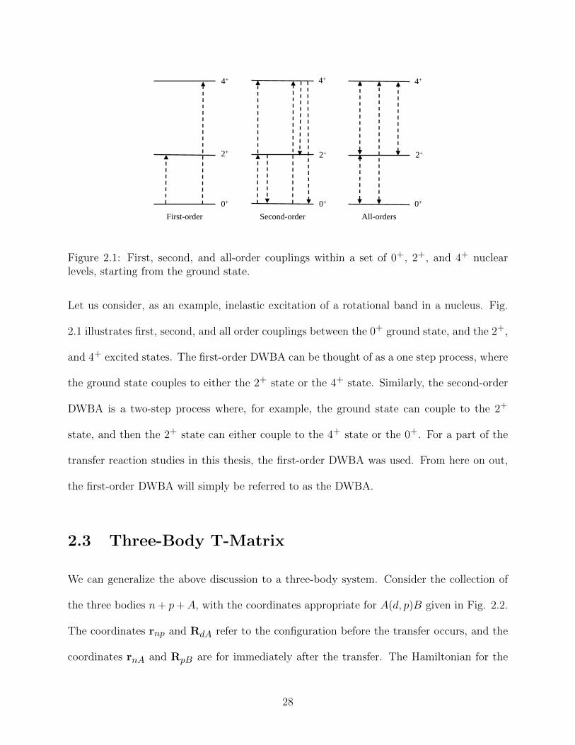
Figure 2.1: First, second, and all-order couplings within a set of 0+, 2+, and 4+

nuclear levels, starting from the ground state. . . . . . . . . . . . . 28

Figure 2.2: The coordinates used in a one particle transfer reaction. . . . . . . 29

Figure 2.3: The coordinates used to calculate the T-matrix for (d, p) transfer. . 34

Figure 2.4: The first four Weinberg States when using a central Gaussian whichreproduces the binding energy and radius of the deuteron groundstate. The inset shows the asymptotic properties of each state. . . . 40

Figure 2.5: The coordinates used for constructing the neutron nonlocal potential.The open dashed circle represents the neutron in a different point inspace to account for nonlocality. . . . . . . . . . . . . . . . . . . . . 42

Figure 2.6: The coordinates used for constructing the system wave function forthe d+ A deuteron scattering state. . . . . . . . . . . . . . . . . . . 44

x

Figure 3.1: Differential elastic scattering relative to Rutherford as a function ofscattering angle. (a) 48Ca(p, p)48Ca at 15.63 MeV with data from [9](b) 208Pb(p, p)208Pb at 61.4 MeV with data from [10]. . . . . . . . . 57

Figure 3.2: Calculated and experimental elastic scattering angular distributionsusing the nonlocal DOM potential. Data for each energy are offset forclarity with the lowest energy at the bottom and highest at the top.Data references in [11]. Figure reprinted from [11] with permission. . 62

Figure 3.3: 49Ca(p, p)49Ca at 50.0 MeV: The solid line is obtained from usingthe Perey-Buck nonlocal potential, the open circles are a fit to thenonlocal solution, and the dotted line is obtained by transforming thedepths of the volume and surface potentials according to Eq. (B.14).Figure reprinted from [12] with permission. . . . . . . . . . . . . . . 65

Figure 4.1: Real and imaginary parts of the Jπ = 1/2− partial wave of the scat-tering wave function for the reaction 49Ca(p, p)49Ca at 50.0 MeV:ψNL (solid line), ψPCF (crosses), and ψloc (dashed line). Top (bot-tom) panel: absolute value of the real (imaginary) part of the scat-tering wave function. Figure reprinted from [12] with permission. . . 72

Figure 4.2: Real and imaginary parts of the Jπ = 11/2+ partial wave of thescattering wave function for the reaction 49Ca(p, p)49Ca at 50.0 MeV.See caption of Fig. 4.1. Figure reprinted from [12] with permission. . 72

Figure 4.3: Ground state, 2p3/2, bound wave function for n+48Ca. φNL (solid

line), φPCF (crosses), and φloc (dashed line). The inset shows thedifference φNL − φPCF . Figure reprinted from from [12] with per-mission. . . . . . . . . . . . . . . . . . . . . . . . . . . . . . . . . . . 74

Figure 4.4: Angular distributions for 49Ca(p, d)48Ca at 50 MeV: Inclusion of non-locality in both the proton scattering state and the neutron boundstate (solid), using LPE potentials, then applying the correction fac-tor to both the scattering and bound states (crosses), using the LPEpotentials without applying any corrections (dashed line), includingnonlocality only in the proton scattering state (dotted line) and in-cluding nonlocality only in the neutron bound state (dot-dashed line).Figure reprinted from [12] with permission. . . . . . . . . . . . . . . 75

Figure 4.5: Same as in Fig. 4.4 but for 49Ca(p, d)48Ca at Ep = 20 MeV. Figurereprinted from [12] with permission. . . . . . . . . . . . . . . . . . . 77

Figure 4.6: Same as in Fig. 4.4 but for 133Sn(p, d)132Sn at Ep = 20 MeV. Figurereprinted from [12] with permission. . . . . . . . . . . . . . . . . . . 77

xi

Figure 4.7: Same as in Fig. 4.4 but for 209Pb(p, d)208Pb at Ep = 20 MeV. Figurereprinted from [12] with permission. . . . . . . . . . . . . . . . . . . 78

Figure 4.8: Angular distributions for elastic scattering normalized to Rutherfordfor protons on 40Ca at Ep = 20 MeV. The elastic scattering withthe DOM potential (solid line), the DOM LPE potential (open cir-cles), the Perey-Buck interaction (dashed line), and the Perey-BuckLPE potential (open squares). The data (closed diamonds) from [13].Figure reprinted from [14] with permission. . . . . . . . . . . . . . . 81

Figure 4.9: Same as in Fig. 4.8 but for Ep = 50 MeV. Data from [15]. Figurereprinted from [14] with permission. . . . . . . . . . . . . . . . . . . 82

Figure 4.10: The real and imaginary parts of the Jπ = 1/2+ partial wave of thescattering wave function for the reaction 40Ca(p, p)40Ca at Ep = 50MeV. This shows the wave function resulting from the DOM poten-tial (solid line) and its LPE potential (dotted line), the Perey-Buckpotential (dashed line) and its LPE potential (dot-dashed line). Thetop (bottom) panel shows the absolute value of the real (imaginary)part of the scattering wave function. Figure reprinted from [14] withpermission. . . . . . . . . . . . . . . . . . . . . . . . . . . . . . . . . 83

Figure 4.11: The neutron ground state 1d3/2 bound wave function for n+39Ca.

Shown is the wave function obtained using the DOM potential (solidline), the Perey-Buck potential (crosses) and the local interaction(dashed line). The inset shows the asymptotic properties of eachwave function. Figure reprinted from [14] with permission. . . . . . 84

Figure 4.12: Angular distributions for the 40Ca(p, d)39Ca reaction at (a) Ep = 20MeV, (b) Ep = 35 MeV, and (c) Ep = 50 MeV. In this figure is thetransfer distribution resulting from using the nonlocal DOM (solidline) and its LPE potential (dotted line), the Perey-Buck potential(dashed line) and the Perey-Buck LPE potential (dot-dashed line).Figure reprinted from [14] with permission. . . . . . . . . . . . . . . 86

Figure 4.13: Absolutes value of the d + A source term when nonlocal and localpotentials are used. (a) d+48Ca at Ed = 50 MeV. (b) d+208Pb atEd = 50 MeV. Both are for the L = 1 and J = 0 partial wave. Figurereprinted from [3] with permission. . . . . . . . . . . . . . . . . . . . 89

Figure 4.14: Absolute value of the d + A source term when nonlocal and localpotentials are used. (a) d+48Ca at Ed = 50 MeV. (b) d+208Pb atEd = 50 MeV. Both are for the L = 6 and J = 5 partial wave. Figurereprinted from [3] with permission. . . . . . . . . . . . . . . . . . . . 90

xii

Figure 4.15: Absolute value of the d+A scattering wave function using the ADWAtheory when nonlocal and local potentials are used. (a) d+48Ca and(b) d+208Pb. Both for the L = 1 and J = 0 partial wave at Ed = 50MeV in the laboratory frame. Figure reprinted from [3] with permis-sion. . . . . . . . . . . . . . . . . . . . . . . . . . . . . . . . . . . . 91

Figure 4.16: Absolute value of the d+A scattering wave function using the ADWAtheory when nonlocal and local potentials are used. (a) d+48Ca and(b) d+208Pb. Both for the L = 6 and J = 5 partial wave at Ed = 50MeV in the laboratory frame. Figure reprinted from [3] with permis-sion. . . . . . . . . . . . . . . . . . . . . . . . . . . . . . . . . . . . 92

Figure 4.17: Angular distributions for (d, p) transfer cross sections. The insetsare the theoretical distributions normalized to the peak of the datadistribution. (a) 48Ca(d, p)49Ca at Ed = 10 MeV with data [16] atEd = 10 MeV in arbitrary units. (b) 132Sn(d, p)133Sn at Ed = 10MeV with data [17] at Ed = 9.4 MeV. (c) 208Pb(d, p)209Pb at 20MeV with data [18] (Circles) and [19] (Squares) at Ed = 22 MeV.Figure reprinted from [3] with permission. . . . . . . . . . . . . . . 95

Figure 4.18: Angular distributions for (d, p) transfer cross sections. The inset isthe theoretical distributions normalized to the peak of the data distri-bution. (a) 48Ca(d, p)49Ca at Ed = 50 MeV with data [20] at Ed = 56MeV. (b) 132Sn(d, p)133Sn at Ed = 50 MeV. (c) 208Pb(d, p)209Pb at50 MeV. Figure reprinted from [3] with permission. . . . . . . . . . 96

Figure 4.19: Comparison of (d, p) transfer cross sections when using the DWBA ascompared to the ADWA. (a) 16O(d, p)17O, (b) 48Ca(d, p)49Ca withdata from [20]. (c) 132Sn(d, p)133Sn. All distributions at Ed = 50MeV. Figure reprinted from [3] with permission. . . . . . . . . . . . 100

Figure 4.20: Comparison of (d, p) angular distributions when using the energyshift method of [21, 22]. (a) 16O(d, p)17O at Ed = 10 MeV (b)40Ca(d, p)41Ca at Ed = 10 MeV (c) 208Pb(d, p)209Pb at Ed = 20MeV. The solid line is when full nonlocality was included in the en-trance channel, dashed line is when the LPE potential was used, dot-dashed line when the CH89 potential [23] was used with the additionalenergy shift quantified in [21], and the dotted line when the CH89 po-tential was used at the standard Ed/2 value. Figure reprinted from[3] with permission. . . . . . . . . . . . . . . . . . . . . . . . . . . . 102

Figure E.1: Differential elastic scattering relative to Rutherfored as a function ofscattering angle. 209Pb(p, p)209Pb at Ep = 50.0 MeV: The solid lineis obtained from NLAT, the dotted line is obtained from NLAT andsetting β = 0.05 fm, and the dashed line is from FRESCO. . . . . 177

xiii

Figure E.2: Differential elastic scattering as a function of scattering angle. 208Pb(n, n)208Pbat Ep = 14.5 MeV: The solid line is obtained a nonlocal calculationusing NLAT, and the dashed line is the nonlocal calculation publishedby Perey and Buck [1]. . . . . . . . . . . . . . . . . . . . . . . . . . 178

Figure E.3: n+48Ca bound wave function, and the deuteron bound wave function.n+48Ca: The solid line is obtained from NLAT, the dotted line isobtained from NLAT and setting β = 0.05 fm, and the dashed line isfrom FRESCO. Deuteron: Dot-dashed line is deuteron bound wavefunction obtained from NLAT, and the open circles are obtained withFRESCO. . . . . . . . . . . . . . . . . . . . . . . . . . . . . . . . 179

Figure E.4: The local adiabatic potential for d+48Ca at Ed = 20 MeV calculatedwith NLAT and with TWOFNR [24]. (a) Real part, (b) Imaginarypart. . . . . . . . . . . . . . . . . . . . . . . . . . . . . . . . . . . . 180

Figure E.5: 48Ca(d, d)48Ca at Ed = 20 MeV. The solid line is when using thelocal adiabatic potential, the dotted line is when doing a nonlocalcalculation with β = 0.1 fm in the nucleon optical potentials, and thedashed line is a calculation done in FRESCO. . . . . . . . . . . . . 181

Figure E.6: 132Sn(d, p)133Sn at Ed = 50 MeV. Solid line is a local DWBA calcula-tion with NLAT, the dashed line is a calculation done with FRESCO.181

Figure E.7: Angular distributions for 208Pb(d, p)209Pb at Ed = 50 MeV obtainedby using different step sizes to calculate the rhs of Eq.(2.49). Thesolid line uses a step size of 0.01 fm, the dashed line a step size of0.03 fm, and the dotted line a step size of 0.05 fm. . . . . . . . . . . 184

Figure E.8: Angular distributions for 208Pb(d, p)209Pb at Ed = 50 MeV obtainedby using different step sizes and values of a cut parameter (CutL) tocalculate the rhs of Eq.(2.49). The solid line uses a step size of 0.01fm with CutL=2, the dashed line a step size of 0.01 fm with CutL=3,and the dotted line a step size of 0.05 fm with CutL=2. . . . . . . . 185

Figure F.1: Neutron and proton spectroscopic factors for 17O and 17F, respec-tively, considering the 16O core in its 0+ ground state and 2+ firstexcited state: (a) 5/2+ ground state and (b) 1/2+ first excited state.Figure reprinted from [25] with permission. . . . . . . . . . . . . . 193

Figure F.2: Ratio of proton and neutron ANCs for 17O and 17F, respectively, in-cluding 16O(0+, 2+): (a) 5/2+ ground state and (b) 1/2+ first excitedstate. Figure reprinted from [25] with permission. . . . . . . . . . . 193

xiv

Chapter 1

Introduction

Since the dawn of nuclear physics, reaction studies have been performed to investigate the

properties of the nucleus. One of the many reasons these studies have been carried out

is to address the overarching goal of nuclear physics. This is to understand where all the

matter in the universe came from and how it was formed. To solve this problem, we not only

need to understand the environments in which nuclear reactions occur, but we also need to

understand the nature of the nuclei undergoing the reactions. This is a daunting task with

hundreds of stable nuclei, and thousands of unstable nuclei known to exist [6].

In Fig. 1.1 the chart of the nuclides is shown with the corresponding proton and neutron

drip lines. The drip line is the point that separates bound from unbound nuclei. The neutron

drip line, for example, defines the point where the addition of a single neutron will make the

resulting nucleus unbound. While an extraordinary amount of progress has been made in

experimentally measuring unstable nuclei, it is remarkable how far the neutron drip line is

expected to extend, and how many nuclei are yet to be discovered.

For many decades, intense experimental and theoretical effort has been put into studying

stable nuclei. While experiments aimed at studying stable isotopes are still performed,

the focus in modern times has shifted towards the study of exotic nuclei. In the context

of understanding the origin of the matter in the universe, exotic nuclei play a crucial role.

While exotic nuclei live for a very short period of time, reactions on exotic nuclei are essential

to creating heavy elements [8]. In certain astrophysical environments, nuclei rapidly capture

1

protons or neutrons, pushing them towards the drip line. These unstable nuclei then β decay

back to the valley of stability. To fully understand the path the nucleosynthesis takes, and

the elements that are produced, we must understand the properties of the exotic nuclei very

far from stability, and the reaction mechanisms of neutrons, protons, or heavier elements on

those exotic nuclei.

Figure 1.1: The chart of the nuclides. The proton drip line is indicated by the line abovethe stable nuclei, and the neutron drip line is indicated below the stable nuclei. The proton(neutron) drip line indicates where the addition of a single proton (neutron) will make theresulting nucleus unbound. Figure reprinted from [6] with permission.

For many nuclear reaction experiments, a good reaction theory is required to extract

reliable information. The same can be said about the potentials we put into our theories. In

fact, the two work hand in hand. An excellent model can be held back by the use of poor

interactions, while the best interaction available will provide little insight when used in a

poor model.

An important part of understanding the properties of nuclei is knowing the spin and parity

assignments of the various energy levels. Single nucleon transfer reactions are an excellent

2

tool for understanding these properties. The protons and neutrons inside a nucleus arrange

themselves in an organized way, roughly following the way levels organize themselves in a

harmonic oscillator potential with a spin-orbit interaction. Filling a shell provides additional

stability. Indicated in Fig. 1.2 (right) are the magic numbers corresponding to the number

of neutrons or protons needed to fill in a shell. The ordering shown in Fig. 1.2 provides a

guide to assigning energy levels. As one moves away from stability there is shell reordering

and different magic numbers emerge.

The use of single nucleon transfer reactions such as (d, p) or (p, d) as a probe to study

nuclear structure began in the early 1950s. Butler realized that the spins and parities of

nuclear energy levels can be obtained from angular distributions, without the need to know

properties of excited states [26]. This fact was reiterated by Huby [27, 28], and later followed

up with theoretical calculations by Bhatia and collaborators [29]. While these early studies

relied on the very simple plane wave Born approximation, it drew considerable attention

to (d, p) reactions as a means to study nuclear structure through the analysis of angular

distributions of transfer reactions.

Since these pioneering studies, the shell structure of nuclei has been studied with the aid

of single nucleon transfer reactions. Of particular interest for this work are the stripping

(d, p) or pickup (p, d) reactions. These types of reactions are an excellent tool for measuring

the energy levels of nuclei, as well as the spin and parity assignments of the corresponding

energy levels. It is transfer reactions such as these which provided much of the structure

information of stable isotopes in the early days of nuclear physics [30, 31, 32, 33, 34, 35].

In Fig. 1.3 we show the dependence of the transfer angular distribution on the transferred

angular momentum for 58Ni(d, p)59Ni at 10 MeV. The transferred angular momentum has

an influence on the shape of the transfer distribution, as well as the location of the peak of

3

Figure 1.2: Typical Nuclear Shell Structure.

the transfer distribution. It is seen that for the s1/2 state the peak occurs at 0, and for

increasing angular momentum transfer the first peak gets shifted to increasing angles. The

oscillations of the transfer distribution can be understood in terms of a diffraction pattern,

analogous to that of a single slit diffraction pattern. With increasing energy the diffraction

pattern is found to have more oscillations. Also, as the beam energy increases, the transfer

distribution gets shifted to more forward angles. The magnitude of the cross section is related

to the Q-value, or energy mismatch, of the reaction. The magnitude of the cross section is

largest when Q = 0, and decreases as energy mismatch increases.

Modern reaction theories have progressed greatly since the 1950s, allowing for more reli-

able nuclear structure information to be extracted from experimental data. The theoretical

4

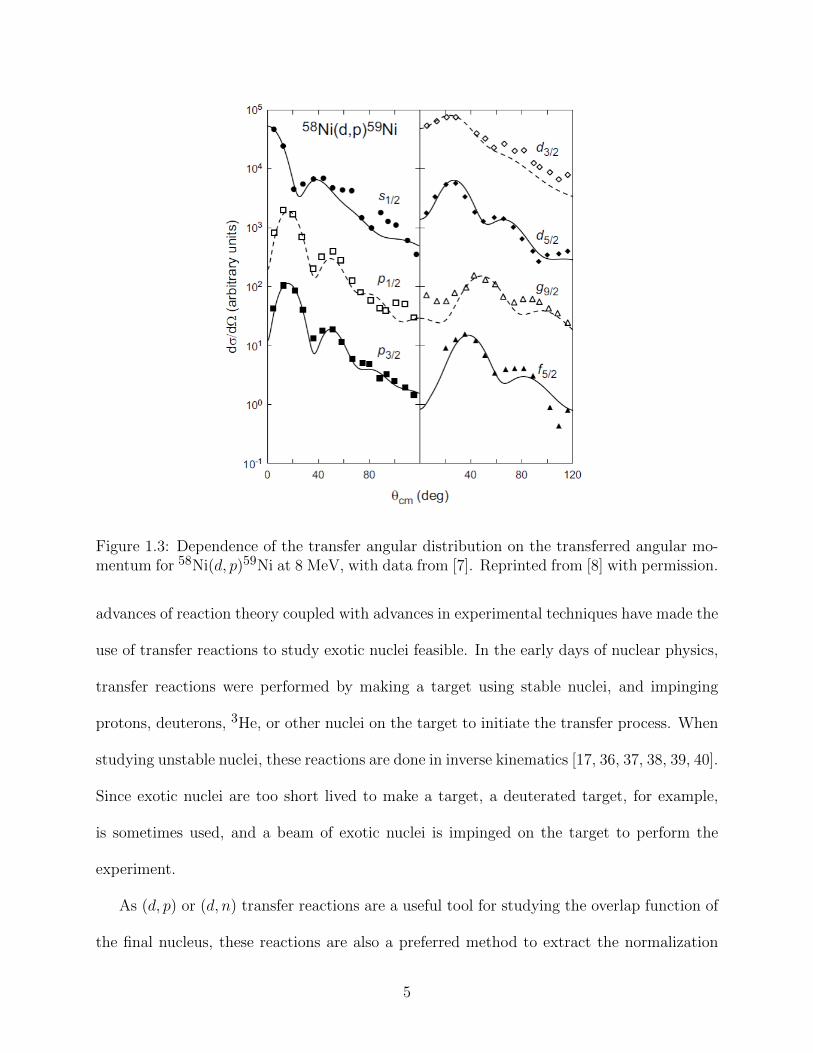
Figure 1.3: Dependence of the transfer angular distribution on the transferred angular mo-mentum for 58Ni(d, p)59Ni at 8 MeV, with data from [7]. Reprinted from [8] with permission.

advances of reaction theory coupled with advances in experimental techniques have made the

use of transfer reactions to study exotic nuclei feasible. In the early days of nuclear physics,

transfer reactions were performed by making a target using stable nuclei, and impinging

protons, deuterons, 3He, or other nuclei on the target to initiate the transfer process. When

studying unstable nuclei, these reactions are done in inverse kinematics [17, 36, 37, 38, 39, 40].

Since exotic nuclei are too short lived to make a target, a deuterated target, for example,

is sometimes used, and a beam of exotic nuclei is impinged on the target to perform the

experiment.

As (d, p) or (d, n) transfer reactions are a useful tool for studying the overlap function of

the final nucleus, these reactions are also a preferred method to extract the normalization

5

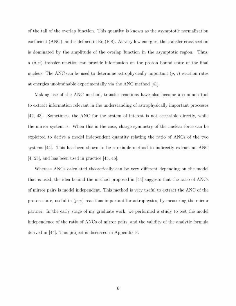
of the tail of the overlap function. This quantity is known as the asymptotic normalization

coefficient (ANC), and is defined in Eq.(F.8). At very low energies, the transfer cross section

is dominated by the amplitude of the overlap function in the asymptotic region. Thus,

a (d, n) transfer reaction can provide information on the proton bound state of the final

nucleus. The ANC can be used to determine astrophysically important (p, γ) reaction rates

at energies unobtainable experimentally via the ANC method [41].

Making use of the ANC method, transfer reactions have also become a common tool

to extract information relevant in the understanding of astrophysically important processes

[42, 43]. Sometimes, the ANC for the system of interest is not accessible directly, while

the mirror system is. When this is the case, charge symmetry of the nuclear force can be

exploited to derive a model independent quantity relating the ratio of ANCs of the two

systems [44]. This has been shown to be a reliable method to indirectly extract an ANC

[4, 25], and has been used in practice [45, 46].

Whereas ANCs calculated theoretically can be very different depending on the model

that is used, the idea behind the method proposed in [44] suggests that the ratio of ANCs

of mirror pairs is model independent. This method is very useful to extract the ANC of the

proton state, useful in (p, γ) reactions important for astrophysics, by measuring the mirror

partner. In the early stage of my graduate work, we performed a study to test the model

independence of the ratio of ANCs of mirror pairs, and the validity of the analytic formula

derived in [44]. This project is discussed in Appendix F.

6

1.1 Nuclear Interactions

The elastic scattering of a nucleon off of a nucleus is a complicated quantum many-body

problem. To solve the problem exactly would require the fully anti-symmetrized many-body

wave function that includes the couplings of the elastic channel to all the other non-elastic

channels available (transfer, inelastic scattering, charge exchange, fusion, fission, etc.). This

is a very difficult problem to solve, and in practice, the scattering process is not solved in this

manner. However, the elastic scattering of a particle from some arbitrary potential, U(R),

is well understood [8, 47]. Assuming that the complicated interaction between some particle

and the nucleus can be represented by a complex mean-field is the basis of the optical model.

In Fig. 1.4 we show the angular distributions for elastic scattering of nucleons off 208Pb at

25 MeV. In panel (a) is n+208Pb, and in panel (b) is p+208Pb. Due to the Coulomb potential,

proton elastic scattering is usually normalized to Rutherford, which is the point-Coulomb

cross section, and always goes to unity at 0. When this is done, the angular distributions

for proton elastic scattering are unitless. The oscillations result from a diffraction pattern

which can be understood qualitatively in a similar way as single slit diffraction. For a larger

target or lower energy, there will be fewer oscillations between 0 and 180, and there will

be more oscillations for a smaller target or a higher energy.

In the optical model, elastic scattering data are fit by varying potential parameters in an

assumed form for U(R). This complex interaction, referred to as the optical potential, is used

to describe the elastic scattering process of the particle off the nucleus, with the imaginary

part taking into account loss of flux to non-elastic channels. Once the optical potential is

defined, it can then be used as an input to a model that describes some other process with the

goal of obtaining an observable other than elastic scattering, such as transfer cross sections.

7

0 30 60 90 120 150 180θ

c.m.

100

101

102

103

104

105

dσ/d

Ω [

mb/

sr]

0 30 60 90 120 150 180θ

c.m.

0.0

0.2

0.4

0.6

0.8

1.0

1.2

1.4

σ/σ R

a) b)

Figure 1.4: Angular distributions for elastic scattering of nucleons off 208Pb at 25 MeV. (a)n+208Pb (b) p+208Pb with differential cross section normalized to Rutherford.

Elastic scattering data for the desired target and energy are often times not available. To

remedy this problem, optical potentials are constructed through simultaneous fits to large

data sets of elastic scattering. These are referred to as global optical potentials. The energy,

target, and projectile dependent parameters are varied to produce a best fit to the entire

data set. The purpose of using a global potential is that one can easily interpolate in order to

obtain a potential for a nucleus in which there is no experimental data available. Obtaining a

potential, and therefore predictions on observables, of un-measured nuclei is a very attractive

feature of using a global potential and is a credit to their success over the decades. It is for

this reason that considerable effort has been put into creating many different global optical

potentials over the years which have received widespread use [48, 23, 49].

Global potentials are a very useful tool for studying nuclear reactions and predicting

observables. However, the way they are constructed leaves out a considerable amount of

physics. Elastic scattering only constrains the normalization of the scattering wave function

outside the range of the interaction. It is not sensitive to the short-range properties of

the wave function. Therefore, the short-range physics is not constrained at all by elastic

8

scattering. Also, much of the elastic scattering data that exists is for stable nuclei. With

the increasing interest of the study of rare isotopes, the extrapolations to exotic nuclei may

not be reliable. It is for this reason that a more physically motivated form for the optical

potential should be pursued.

All widely used global optical potentials are local. However, when derived from a many-

body theory, the resulting optical potential is nonlocal. The strong energy dependence of

global potentials is assumed to account for the nonlocality that is neglected. With increasing

interest in microscopically derived optical potentials, it is becoming necessary to investigate

the validity of the local assumption, and develop methods to incorporate nonlocal potentials

into modern reaction theories.

1.2 Nonlocality

It has long been known that the optical potential is nonlocal [50]. In the Hartree-Fock the-

ory, the existence of an exchange term introduces an explicit nonlocal potential [51]. For

scattering, the complicated coupling of the elastic channel to all other non-elastic channels

accounts for another significant source of nonlocality [52, 53]. These two sources of nonlo-

cality, anti-symmetrization and channel couplings, have been known and studied for decades

(e.g. [54]).

As a physical example, consider a deuteron impinging on a target, and let R and R’

locate the center of the deuteron relative to the center of the target. Let’s say that the

deuteron breaks up at R′ as it approaches the target. The deuteron can then propagate

through space in its broken up state, then recombine to form the deuteron again at R.

This process is depicted in Fig. 1.5. Such a process would constitute a channel coupling

9

nonlocality. This will result in a potential of the form V (R,R′) since the interaction at a

given point is dependent on the value of the potential and the scattering wave function at

all other points in space.

k

Figure 1.5: An example of a channel coupling nonlocality. In this case, the deuteron is im-pinged on some target. The channel coupling nonlocality results from the deuteron breakingup as it approaches the nucleus, propagating through space in its broken up state, and thenrecombining to form the deuteron again.

As another example, consider a single nucleon scattering off a nucleus. Since the system

wave function is a fully anti-symmetric many-body wave function, it is not guaranteed that

the projectile in the incident channel is the same particle as the one in the exit. The Pauli

principle also plays a role when the projectile is propagating through the nuclear medium,

and most notably has the effect of reducing the amplitude of the wave function in the nuclear

interior. All of these effects will manifest in a potential of the form V (R,R′).

1.2.1 Microscopic Optical Potentials

This work is not concerned with constructing a microscopic optical potential, but rather

with using current phenomenological nonlocal optical potentials, and studying the effects of

nonlocality on transfer observables. However, it is important to understand the considerable

10

amount of effort that has been put forth in recent decades to construct optical potentials

from microscopic theories. In this thesis we will demonstrate that nonlocality is an important

feature of the nuclear potential that must be considered explicitly. Moving forward, the

development of ab-initio many-body theories offer the promise of realistic microscopic optical

potentials. The methods outlined here will be the tools for future studies.

Several studies have been made to construct a microscopically based optical potential. In

the pioneering work of Watson [55, 56], and later refined by Kerman, McManus, and Thaler

(KMT) [57], the theory of multiple scattering was developed, where the optical potential to

describe elastic scattering is constructed in terms of the amplitudes for the scattering of the

incident particle by the individual neutrons and protons in the target nucleus. This theory

for constructing the optical potential is limited to relatively high energies (> 100 MeV).

Deriving the multiple scattering expansion of the KMT optical potential is a complicated

task, but has been done successfully, such as for 16O [58].

The optical potential can also be identified with the self-energy, as first indicated by Bell

and Squires [50]. Hufner and Mahaux studied the optical potential in great detail through

use of a systematic expansion of the self-energy within the Greens function approach to the

many-body problem [59]. This approach is analogous to the Bethe-Brueckner expansion

for the calculation of the binding energy [60]. This formulation of the optical potential in

terms of the self-energy is attractive as it is suitable for both intermediate and high energy

scattering, and reduces to the expressions of multiple scattering theory at high energies.

It is through the connection to the self-energy that Jeukenne, Lejeune, Mahaux (JLM)

formulated their optical model potential for infinite nuclear matter [61]. In infinite nuclear

matter, the concept of a projectile and target lose their meaning. Instead, a potential energy

and a lifetime for a quasiparticle state obtained by creating a particle or hole with momentum

11

k above the correlated ground state is defined. Later, the JLM approach was extended to

finite nuclei using a local density approximation [62].

The link between the self-energy and the optical potential was further explored by Ma-

haux and Sartor [63]. This implementation is known as the dispersive optical model (DOM).

The advantage of this method is that it provides a link between nuclear reactions and nu-

clear structure through a dispersion relation. In recent years, a local version of the DOM

was introduced for Calcium isotopes [64], and a nonlocal DOM was subsequently developed

for 40Ca [65, 11]. Transfer reaction studies have shown that the local DOM is able to de-

scribe transfer cross sections as well as or better than global potentials [66], and that the

nonlocal DOM can significantly modify the shell occupancy, or spectroscopic factor, of the

states populated in transfer reactions [14].

Various other techniques exist which construct an optical potential through the self-

energy using modern advances in nuclear theory. Making use of the progress that has been

achieved, Holt and collaborators constructed a microscopic optical potential from the self-

energy for nucleons in a medium of infinite isospin-symmetric nuclear matter within the

framework of chiral effective field theory [67].

The two sources of nonlocality, channel coupling and anti-symmetrization, have been

studied over the years by numerous authors [54, 68, 69] to name only a few. Many of

these studies derive the nonlocal potential using some microscopic theory, then compare

the potential obtained to commonly used phenomenological nonlocal potentials. Such was

done in [54] where the multichannel algebraic scattering (MCAS) method [70] was used

to obtain the nonlocal potential resulting from channel coupling. The resulting nonlocal

potential was found to be very different from the simple Gaussian nonlocalities assumed

in phenomenological potentials. However, the MCAS method is only suitable for very low

12

energy projectiles, where just a few excited states are relevant to the coupling, and thus, can

be explicitly coupled together to generate the channel coupling nonlocal potential.

1.2.2 Phenomenological Nonlocal Optical Potentials

The formalism to develop a microscopic optical potential is complicated, and requires con-

siderable computation time to implement. However, constructing a nonlocal potential phe-

nomenologically provides a practical alternative to construct a nonlocal potential applicable

for widespread use. The seminal work of Perey and Buck, [1], was the first attempt to con-

strain the parameters of a nonlocal potential through fits to elastic scattering data. This

work was done in the sixties, but it is still the most commonly referenced nonlocal optical

potential. In the late seventies, Giannini and Ricco constructed a phenomenological nonlo-

cal optical potential, [71, 72]. In that work, the potential parameters were constrained with

fits to a local form, then a transformation formula was used to obtain the nonlocal poten-

tial. Very recently, Tian, Pang, and Ma (TPM) introduced a third nonlocal global optical

potential, [2]. These three works are to our knowledge the only attempts to construct a

phenomenologial nonlocal global optical potential.

A common feature of using a nonlocal potential is that the amplitude of the wave function

is reduced in the nuclear interior as compared to the wave function resulting from using a

local potential. Numerous studies have been performed to investigate this effect, and to

find ways to correct for it [73, 74, 75]. These studies were focused on potentials of the

form of the phenomenological Perey-Buck nonlocal potential. A local equivalent potential

to the nonlocal potential should formally exist. Attempts have been made to find this local

equivalent potential [76, 77]. In nearly all these cases, the Perey-Buck form for the nonlocal

potential was assumed.

13

1.2.3 Solving Nonlocal Equations

While the theoretical foundation for constructing nonlocal potentials has been around for

many decades, the broad application of nonlocal potentials in the field of nuclear reactions

has never come to fruition. With a nonlocal potential, the Schrodinger equation transforms

from a differential equation to an integro-differential equation. Therefore, the most straight-

forward way to solve the equation is through iterative methods, which dramatically increases

the computational cost.

Since the knowledge of nonlocality dates back to the 1950s when computer power was

much more limited than today, the preferred method was to include nonlocality approxi-

mately through a correction factor [73, 74, 75]. However, several methods now exist that

improve the efficiency of the basic iteration scheme. Kim and Udagawa have presented a

rapid method using the Lanczos technique [78, 79]. A method by Rawitscher uses either

Chebyshev or Sturmian functions as a basis to expand the scattering wave function [80].

Also, an improved iterative method has been proposed by Michel [81].

Computation time is no longer an issue. In this work, we used an iterative method out-

lined in Appendix A to solve the integro-differential equation. This is, by far, the easiest, but

definitely not the most efficient way to solve the equation. Since the increase in computation

time is minimal, pursuing a faster way was not a priority and will be pursued at a later time.

If one desired to construct their own global nonlocal potential by fitting large amounts of

elastic scattering data, it would be advantageous to further optimize our technique.

14

1.3 Motivation for present work

In this work, we would like to describe single nucleon transfer reactions involving deuterons

while using nonlocal optical potentials. Ever since the early days of nuclear physics, right

up to the modern day, the distorted wave Born approximation (DWBA) has been a common

theory used to analyze data from transfer reaction experiments [82, 83]. In the DWBA, the

transfer process is assumed to occur in a one-step process, and an optical potential fitted to

deuteron elastic scattering is used to describe the deuteron scattering state. The shortcoming

of the DWBA is that the deuteron is loosely bound, so it is likely that the deuteron will

breakup as it approaches the nucleus. Not taking deuteron breakup into account explicitly

can have a significant effect on transfer cross sections. In all known implementations of the

DWBA to describe transfer cross sections, local deuteron optical potentials have been used.

These deuteron optical potentials were obtained either by fitting a single elastic scattering

angular distribution, or using a global parameterization such as that from Daehnick [84].

In order to include deuteron break up explicitly, it is necessary to include the n−p degrees

of freedom. This then requires solving the n + p + A three-body problem. A three-body

approach was introduced in the zero range approximation by Johnson and Soper [85], and

later extended to include finite range effects by Johnson and Tandy [86]. This is known as

the adiabatic distorted wave approximation (ADWA). A recent systematic study of (d, p)

reactions within the formalism of [86] shows the importance of finite range effects [87]. In

these theories the deuteron scattering state is treated as a three-body problem, composed

of n + p + A. The breakup of the deuteron is included explicitly, and the input potentials

are neutron and proton optical potentials, which are much better constrained than deuteron

optical potentials. In this sense, ADWA is a more advanced theory than the DWBA with

15

the added advantage that nucleon optical potentials exist in a nonlocal form. Therefore, in

this work the explicit inclusion of nonlocality in single nucleon transfer reactions within the

ADWA will be pursued.

As mentioned before, nonlocality in (d, p) transfer reactions has traditionally been in-

cluded approximately through a correction factor. This is the method exploited in com-

monly used transfer reaction codes such as TWOFNR [24]. The bound and scattering wave

functions are calculated using a suitable local potential, normally a global potential for elas-

tic scattering and a mean field reproducing the experimental binding energy for the bound

state. The correction factor used implies that the nonlocality assumed is of the Perey-Buck

form. From microscopic calculations, it is known that a single Gaussian is not sufficient to

take into account the complex nature of nonlocality [54]. Therefore, not only is this method

of including nonlocality not accurate, but it is limited to a form for the nonlocality that may

not adequately represent the true nonlocality in the nuclear potential.

Recently, some attempts have been made to include nonlocality within the adiabatic

model by introducing an energy shift to the optical potentials used to calculate the scattering

wave functions [22, 21]. This method is very attractive as all local codes which calculate

(d, p) transfer can still be used without modification. However, the adequacy of this energy

shift to take nonlocality into account must be quantified. Another limitation of this method

is that it relies on energy independent nonlocal nucleon optical potentials assumed to have

the Perey-Buck form.

While the existence of nonlocality in the optical model has been known for many decades,

not many calculations of transfer reactions with the explicit inclusion of nonlocality have ever

been performed. While the approximate ways to correct for nonlocality are common, it is

not known if these approximate methods are sufficient. The method of constructing local

16

optical potentials through fits to elastic scattering data has been practical and useful, but

since elastic scattering does not constrain the short range nonlocalities present in the nuclear

potential, it is unlikely this approach to constructing the optical potential will be reliable

when moving towards exotic nuclei. Also, it must be understood how other observables are

affected due to the way in which the optical potentials are constructed.

The goal of this thesis is to study the explicit inclusion of nonlocality on single nucleon

transfer reactions involving deuterons. Since nonlocality has either been ignored or included

approximately in nearly all reaction calculations for over half a century, the effect of neglect-

ing nonlocaly on reaction observables must be quantified. Also, the quality of the commonly

used approximate techniques need to be assessed. For this purpose we extend the formalism

of the ADWA to include nonlocality. Finally, with renewed interest in microscopic optical

potentials, the formalism must be kept general so that nonlocal potentials of any form can

be used.

In this thesis, we will first test the concept of the correction factor using the Perey-Buck

potential. This will be done by performing DWBA calculations of (p, d) reactions on a wide

range of nuclei and energies. The correction factor will be applied to the proton scattering

state, and the neutron bound state in the entrance channel. We will then include nonlocality

explicitly in the entrance channel in order to quantify the adequacy of the correction factor

to account for nonlocality. For this part of the study, a local deuteron optical potential will

be used to describe the deuteron scattering state within the DWBA.

Since it is well known that deuteron breakup plays an important role in describing the

reaction dynamics, it is crucial to incorporate nonlocality into a reaction theory that ex-

plicitly includes deuteron breakup. Thus, we chose to extend the formalism of the ADWA

to include nonlocal potentials. Also, since the Perey-Buck form for the nonlocality is not

17

consistent with microscopic calculations, the formalism was kept general so that it can be

used with a nonlocal potential of any form that may result from a microscopic calculation.

Finally, through a systematic study, the effect of ignoring nonlocality in the optical

potential on transfer observables can be quantified. We will choose a range of nuclei and

energies, and perform calculations of (d, p) transfer reactions using nonlocal potentials in

both the entrance and exit channels. The resulting cross sections will be compared to cross

sections generated from local phase equivalent potentials in order to quantify the effect of

neglecting nonlocality in the optical potential.

1.4 Outline

This thesis is organized in the following way. In chapter 2 we will present the necessary

theory. We will begin with a discussion of elastic scattering, and the two-body T-matrix.

We will extend the two-body T-matrix to three-bodies. Then we will introduce the adiabatic

distorted wave approximation, and finally extend this theory to include nonlocal potentials.

In chapter 3 we will discuss optical potentials. First we will introduce the concept of a global

optical potential, then turn our attention to nonlocal potentials. We will introduce Perey-

Buck type potentials, and the corresponding correction factor. We will then describe the

Giannini-Ricco potential and the DOM nonlocal potential. Last there will be a discussion

of local equivalent potentials. In Chapter 4 we will present our results beginning in Sec. 4.2

with a discussion of (p, d) reactions using the Perey-Buck potential in the entrance channel

within the DWBA. In Sec. 4.3 we compare the effects of including the DOM potential and

the Perey-Buck potential in the entrance channel of (p, d) reactions using the DWBA. Lastly,

in Sec. 4.4 we study (d, p) transfer reactions within the ADWA while including nonlocality

18

consistently. Finally, in Chapter 5 we will draw our conclusions and discuss the outlook for

future work.

Some of the work developed during this thesis, while critical, is too technical to present

in the main body. We have thus collected that information in the following appendices.

In Appendix A we discuss the method by which we solve the scattering and bound state

nonlocal equations. In Appendix B we derive the correction factor that is applied to wave

functions resulting from a local potential in order to account for the neglect of nonlocality.

In Appendix C we derive the nonlocal adiabatic potential, and in Appendix D we derive the

partial wave decomposition of the T-matrix used to calculate transfer reaction cross sections.

In Appendix E we go over some checks to ensure the accuracy of the code I developed to

compute transfer cross sections, NLAT (NonLocal Adiabatic Transfer). In Appendix F,

we discuss a method to extract astrophysically relevant ANCs using the concept of mirror

symmetry. While Appendix F is a research project of relevance to the field that stands on

its own [25], it does not fit the theme of the thesis. Therefore, we chose to include it as a

separate appendix.

19

Chapter 2

Reaction Theory for the Transfer of

Nucleons

Elastic scattering is the anchor of many reaction theories since elastic scattering wave func-

tions are often times inputs to these theories, and are used to calculate quantities such as

transfer cross sections. Elastic scattering is also the primary means by which we construct

the nuclear potential. Therefore, for reaction theory to make useful predictions, we must

have a good understanding of elastic scattering.

The theoretical study of transfer reactions commonly uses the distorted-wave Born ap-

proximation (DWBA). In this theory, the transfer process is assumed to be a single step, and

the breakup of the deuteron is included implicitly through the deuteron optical potential.

The deuteron is loosely bound, and is likely to breakup during the course of the reaction.

Therefore, not including the breakup of the deuteron explicitly is known to be inaccurate

[88]. Despite breakup not being included explicitly, the DWBA theory is still commonly

used to describe transfer reactions due to its simplicity and the legacy of codes available.

Modern reaction theories that incorporate breakup begin with the three-body picture

of the process. The three bodies are the neutron and the proton making up the incident

deuteron, and the target nucleus. A practical method for including deuteron breakup was

introduced by Johnson and Tandy [86]. This method is usually referred to as the adiabatic

20

distorted-wave approximation (ADWA). The ADWA has been benchmarked with more ad-

vanced techniques [89, 90], and shown to be competitive. In [89], (d, p) angular distributions

for the ADWA and the exact Faddeev method are compared. It was found that the results

from the ADWA are within 10% of the full solution at forward angles, demonstrating that

the ADWA is a reliable and practical method for calculating angular distributions of transfer

reactions. The ADWA theory will be the focus of this work.

An attractive feature of the ADWA is that it includes breakup explicitly, and also relies

on nucleon optical potentials, which are much better constrained than the deuteron optical

potentials used in the DWBA. In all known uses of the ADWA, local nucleon optical po-

tentials were used. However, recent studies have shown that the nonlocality of the nuclear

potential can have a significant impact on transfer cross sections [91, 12, 14]. Thus, it has

become necessary to extend the ADWA formalism to include nonlocal potentials [3].

2.1 Elastic Scattering

To describe elastic scattering distributions, we begin by solving the partial wave decomposed

Schrodinger equation

[−~2

2µ

(∂2

∂R2− L(L+ 1)

R2

)+ UN (R) + VC(R)− E

]ψα(R) = 0, (2.1)

with UN (R) being some short-range nuclear potential, VC the Coulomb potential, µ the

reduced mass of the projectile target system, and E the projectile kinetic energy in the center

of mass frame. Here, α = LIpJpIt is a set of quantum numbers that define each partial

21

wave, where L is the orbital angular momentum between the projectile and the target, Ip

and It are the spin of the projectile and target respectively, and Jp is the angular momentum

resulting from coupling the orbital angular momentum with the spin of the projectile. In

the asymptotic limit where the nuclear potential goes to zero, the scattering wave function

takes the form

ψα(R) =i

2

[H−L (ηL, kR)− SαH

+L (ηL, kR)

], (2.2)

where η = Z1Z2e2µ/~2k is the Sommerfeld parameter, k is the wave number, Sα is the

scattering matrix element (S-matrix), andH− andH+ are the incoming and outgoing Hankel

functions [92], respectively. For neutrons, η = 0. The theoretical scattering amplitude for

elastic scattering is related to the S-Matrix by

fµpµtµpiµti(θ) = δµpµpi

δµtµtifc(θ) +

2πi

ki

∑LiLJpiJpMpiMpMiJT

CJpiMpiLiMiIpiµpi

CJtotMtotJpiMpiIti

µti

× CJpMpLMIpµp

CJtotMtotJpMpItµt

YLM (k)Y ∗LiMi(ki)

× (1− Sα) ei(σL(ηα)+σLi

(ηαi))

(2.3)

with µpi and µti being the projections of the spin of the projectile and target, respectively,

before the scattering process, while µp and µt are the spin projections after the scattering

process. In this equation, fc is the point Coulomb scattering amplitude:

22

fc(θ) = − η

2k sin2(θ/2)exp

[−iη ln(sin2(θ/2)) + 2iσ0(η)

], (2.4)

with the Coulomb phase given by σL(η) = argΓ(1 + L+ iη).

The Sα are determined by matching a numerical solution of Eq.(2.1) to the known asymp-

totic form (2.2). This is done by constructing the R-Matrix, which is simply an inverse

logarithmic derivative.

Rα =1

Rmatch

H−L − SαH+L

H−L′ − SαH

+L′ (2.5)

with the primes indicating derivatives with respect to R. The R-Matrix is evaluated at

some matching point outside the range of the nuclear interaction, denoted by Rmatch. The

R-matrix uniquely determines the S-matrix by

Sα =H−L −RmatchRαH

−L′

H+L −RmatchRαH

+L′ . (2.6)

Once the S-matrix for each partial wave is calculated, the theoretical differential cross

section, which is the quantity that is compared with experiment, is obtained by summing

the squared magnitude of the scattering amplitude over the final m-states, and averaging

over the initial states:

23

dσ

dΩ=

1

Ipi Iti

∑µpµtµpiµti

∣∣∣fµpµt,µpiµti (θ)∣∣∣2 (2.7)

2.2 Two-Body T-Matrix

We would like to find the transition amplitude (T-matrix) for a (d, p) transfer reaction. Before

we get to transfer reactions, let us first consider the T-matrix for two-body scattering, such

as elastic scattering. The discussion of Sec. 2.1 formulated elastic scattering in terms of an

S-matrix. This is the way most codes solve elastic scattering. Another way of formulating

elastic scattering is in terms of the T-matrix, and leads to a natural generalization to three-

body scattering, which is the case for d+ A reactions.

We begin with a partial wave decomposed two-body coupled channel equation [8]

[−~2

2µ

(d2

dR2− L(L+ 1)

R2

)+ Vc(R)− E

]ψα(R) = −

∑α′〈α|V |α′〉ψα′(R

′). (2.8)

The T-matrix is an important quantity as it gives the amplitude of the outgoing wave after

scattering. In Eq.(2.2) we wrote the asymptotic form of the scattering wave function in

terms of the S-matrix. We can write an equivalent expression for the asymptotic form of the

wave function in terms of the T-matrix

ψααi(R)→ δααiFLi(ηL, kR) + TααiH+L (ηL, kR), (2.9)

24

where Fα(R) is the regular Coulomb function, and again, H+ is the out going Hankel

function. If U = 0 then T = 0. The goal is thus to find an expression for the T-matrix.

Using Green’s function techniques, the T-matrix for two-body scattering is given by [8]

Tααi = − 2µ

~2k〈φ(−)|V |Ψ〉, (2.10)

where φ is the homogeneous solution when no coupling potentials are present, µ is the

reduced mass of the two-body system, and k is the wave number. The (−) superscript

indicates that φ(−) has incoming spherical waves as the boundary condition. φ(−) is thus

the time reverse of φ. The complex conjugation implied in the bra-ket notation cancels the

complex conjugation implied in the (−).

Often times, we can decompose V into two parts so that V = U1 + U2. We would like

to calculate the T-matrix for the transition when two potentials are present, and derive

the two-potential formula. We begin by writing the T-matrix substituting in the separated

expression for V

−~2k2µ

T1+2 =

∫φ (U1 + U2)ψdR. (2.11)

Using these two potentials, we can define various functions. φ is the free field solution,

χ is the solution distorted by U1 only, and ψ is the full solution. These are related to each

other through the relations

25

[E − T ]φ = 0

χ = φ+ G0U1χ

ψ = φ+ G0(U1 + U2)ψ

= χ+ G1U2ψ, (2.12)

with the two Green’s functions given by

G0 = [E − T ]−1

G1 = [E − T − U1]−1 . (2.13)

Using these relations, we can rewrite the T-matrix as

−~2k2µ

T1+2ααi

=

∫ [χ(U1 + U2)ψ − (G0U1χ)(U1 + U2)ψ

]dR

=

∫[φU1χ+ χU2ψ]dR

= 〈φ(−)|U1|χ〉+ 〈χ(−)|U2|ψ〉.

(2.14)

Consider the elastic scattering of protons as an illustrative example. In this case, U1 could

be the Coulomb potential, and U2 could be the nuclear potential. The first term would be the

Coulomb scattering amplitude, fc(θ), and the second term would be the Coulomb-distorted

26

nuclear amplitude fn(θ). Thus, the nuclear scattering amplitude when Coulomb is present

is not simply the amplitude due to the short-ranged nuclear forces alone, but from the effect

of Coulomb on top of nuclear. From these scattering amplitudes we obtain the differential

elastic cross section by calculating |fc(θ)+fn(θ)|2. This is used in our studies for computing

elastic scattering of charged particles.

2.2.1 Born Series

Using Eq.(2.14), and the implicit form for ψ in Eq.(2.12), we can, by iteration, form what is

known as the Born series:

T(1+2)ααi

= T(1) + T2(1)

= T(1) − 2µ

~2k

[〈χ(−)|U2|χ〉+ 〈χ(−)|U2G1U2|χ〉+ . . .

]. (2.15)

Truncating the series after the first term is known as the first-order distorted-wave Born

approximation (DWBA).

The DWBA is particularly useful when we are describing some kind of transition. If U1

is a central optical potential for all non-elastic channels, it cannot cause the transition since

central potentials are not able to change the quantum numbers of the scattered particle,

or change their energy. When this is the case, T(1) = 0, and we get an expression for the

T-matrix to describe the transition from an incoming channel αi to an exit channel α 6= αi.

TDWBAααi

= − 2µα~2kα

〈χ(−)α |U2|ψαi〉 (2.16)

27

4+ 4+ 4+

2+ 2+ 2+

0+ 0+ 0+

First-order Second-order All-orders

Figure 2.1: First, second, and all-order couplings within a set of 0+, 2+, and 4+ nuclearlevels, starting from the ground state.

Let us consider, as an example, inelastic excitation of a rotational band in a nucleus. Fig.

2.1 illustrates first, second, and all order couplings between the 0+ ground state, and the 2+,

and 4+ excited states. The first-order DWBA can be thought of as a one step process, where

the ground state couples to either the 2+ state or the 4+ state. Similarly, the second-order

DWBA is a two-step process where, for example, the ground state can couple to the 2+

state, and then the 2+ state can either couple to the 4+ state or the 0+. For a part of the

transfer reaction studies in this thesis, the first-order DWBA was used. From here on out,

the first-order DWBA will simply be referred to as the DWBA.

2.3 Three-Body T-Matrix

We can generalize the above discussion to a three-body system. Consider the collection of

the three bodies n+ p+A, with the coordinates appropriate for A(d, p)B given in Fig. 2.2.

The coordinates rnp and RdA refer to the configuration before the transfer occurs, and the

coordinates rnA and RpB are for immediately after the transfer. The Hamiltonian for the

28

three bodies is given by

H = Trnp + TRdA+ Vp(rnp) + Vt(rnA) + UpA(RpA), (2.17)

where UpA(RpA) is the core-core optical potential. We can equivalently express the two

kinetic energy terms as Trnp + TRdA= TrnA + TRpB

. This allows us to write two different

internal Hamiltonians for the bound states, Hd = Trnp +Vp(rnp) and HB = TrnA +Vt(rnA).

Thus, we can write the Hamiltonian in two ways, called the post and the prior form

n

p A

d = n+p

B = n+A

rnp

RdA rnARpB

RpA

Figure 2.2: The coordinates used in a one particle transfer reaction.

H = Hprior = TRdA+ Ui(RdA) +Hp(rnp) + Vi

= Hpost = TRpB+ Uf (RpB) +Ht(rnA) + Vf , (2.18)

where Ui,f are the entrance and exit channel optical potentials, respectively, and the Vi,f

interaction terms are given by

29

Vi = Vt(rnA) + UpA(RpA)− Ui(RdA)

Vf = Vp(rnp) + UpA(RpA)− Uf (RpB). (2.19)

For (d, p) reactions it is advantageous to work in the post form. In such a case, we see

that UpA(RpA)− UpB(RpB) ≈ 0. This term is called the remnant term and approximately

cancels for all but light targets. This is because the optical potentials between p + A and

p+ (A+ 1) are not likely to be significantly different. We demonstrate that the remnant can

be neglected in Sec. 4.1.1.

Just like in the case of elastic scattering, the differential cross section for an A(d, p)B

reaction is found by summing the squared magnitude of the scattering amplitude over the

final m-states, and averaging over initial states. The T-matrix is related to the scattering

amplitude by

fµAMdµpMB(kf ,ki) = −

µf

2π~2

√vfviTµAMdµpMB

(kf ,ki), (2.20)

where the subscript i(f) represents the initial (final) state, µf is the reduced mass, and v

is the velocity of the projectile. Here, µA, Md, µp, and MB are the projection of the spin

of the target in the entrance channel, the deuteron, the proton, and the target in the exit

channel, respectively.

We would like to find the T-matrix for A(d, p)B reactions. Using the post representation

for the Hamiltonian, Eq.(2.18), and the two-potential formula, Eq.(2.14), we can identify

30

U1 = Uf (RpB) + Vt(rnA) and U2 = Vf . Since Uf (RpB) + Vt(rnA) produces the elastic

scattering state of p + B, it cannot cause the transfer transition. Therefore, T(1) = 0. As

a result, T2(1) is the only non-zero term. In our notation, the exact T-matrix for a given

projection of angular momentum in the post form is:

TpostµAMdµpMB

(kf ,ki) = 〈ΨµpMBkf

|Vnp + ∆|ΨµAMdki

〉. (2.21)

The remnant term ∆ = UpA − UpB is negligible for all but light targets. The ket in Eq.

(2.21) for the T-matrix is the full three-body wave function for n + p + A, while the bra

is the product of a proton distorted wave and the n + A bound state wave function. As

a first approximation, we can approximate the ket as a product of a deuteron bound state

and a deuteron distorted wave. This is the well known distorted wave Born approximation

(DWBA). In this case, the ket is given by

|ΨMdµAki

〉 = ΞIAµA(ξA)φji(rnp)χ

(+)i (ki, rnp,RdA, ξp, ξn), (2.22)

where ΞIAµA(ξA) is the spin function for the target, with spin IA and projection µA. φji(rnp)

is the radial wave function for the bound state, which in this case is the deuteron, and ji is

the angular momentum resulting from coupling the spin of the fragment in the bound state

(the neutron) to the orbital angular momentum between the fragment and the core. The

distorted wave, χ(+)i , is given by

31

χ(+)i (ki, rnp,RdA, ξp, ξn) =

4π

ki

∑LiJPi

iLieiσLi

JPiJd

χLiJpi(RdA)

RdA(2.23)

×

YLi(ki)⊗

ΞIp(ξp)⊗Y`i(rnp)⊗ ΞIn(ξn)

ji

Jd

⊗ YLi(RdA)

JPi

JdMd

,

where ΞIp(ξp) and ΞIn(ξn) are the spin functions for the proton and neutron respectively,

with spin Ip = In = 12 . The spin of the deuteron is given by Jd = 1, and the spin of the

deuteron coupled to the orbital angular momentum between the deuteron and the target, Li,

gives the total projectile angular momentum, JPi . The spherical harmonics, YL, are defined

with the phase convention that has a built in factor of iL. Therefore, YL = iLYL with YL

defined on p.133 of the book [93]. The hatted quantities are given by J =√

2J + 1. The

function χLiJPi(RdA) satisfies the equation

[− ~2

2µi

(∂2

∂R2dA

− Li(Li + 1)

R2dA

)+ UdA + V SO1LiJPi

+ VC(RdA)− Ed

]χLiJPi

(RdA) = 0,

(2.24)

where V SO is the spin-orbit potential, and VC is the Coulomb potential. UdA is a deuteron

optical potential. For the bra we have

〈ΨµpMBkf

| =

ΞIA

(ξA)⊗Y`f

(rnA)⊗ ΞIn(ξn)jf

∗JBMB

φjf (rnA)χ(−)∗f (kf ,RpB)

(2.25)

32

where φjf (r) is the n + A bound state radial wave function, jf is the angular momentum

of the bound state resulting from coupling the spin of the neutron to the orbital angular

momentum of the bound state, `f , while JB is the total angular momentum of the final

nucleus, B. The exit channel distorted wave is given by

χ(−)∗f (kf ,RpB , ξp) =

4π

kf Ip

∑LfJPf

i−Lf e

iσLf JPf

χLfJPf(RpB)

RpB

×

YLf (kf )⊗

ΞIp(ξp)⊗ YLf (RpB)JPf

Ipµp

(2.26)

and the function χLfJPf(RpB) satisfies

[− ~2

2µf

(∂2

∂R2pB

−Lf (Lf + 1)

R2pB

)+ UpB + V SOIpLfJPf

+ VC(RpB)− Ep

]χLfJPf

(RpB) = 0

(2.27)

with UpB being the proton optical potential in the exit channel.

We need to do a partial wave decomposition of the T-matrix, Eq.(2.21), so that we can

calculate the scattering amplitude, Eq.(2.20), and hence, the cross section, in a numerically

efficient way. We show in Appendix D that for a general `i and `f relative orbital angular

momentum in the initial and final bound states, the partial wave decomposition of the T-

matrix is given by

33

θ

A

p

B

d

n

z

x

Figure 2.3: The coordinates used to calculate the T-matrix for (d, p) transfer.

TQMQmf= C

∑K

∑LiJPi

∑LfJPf

AK,LiJPi

LfJPfQMQmf

(kf )IK,LiJPi

LfJPf , (2.28)

where phase and statistical factors are collected in

C =32π3In

Ipkikf

(−)3Ip+ji+Jd+2jf

jijf, (2.29)

angular momentum couplings are mostly put in,

34

AK,LiJPi

LfJPfQMQmf

(kf ) =(−)K

K〈`f `i(K)InIn(0)KM |`f In(jf )`iIn(ji)KM〉

×∑LiJPi

∑LfJPf

i3Li+Lf+`f+`ie

i(σLi+σLf

)LiLf JPi JPf

×〈IpJd(ji)LfLi(K)jfmf |IpLf (JPf)JdLi(JPi)jfmf 〉

×∑g

〈LfLi(g)JPfJPi(jf )QMQ|LfJPf (Ip)LiJPi(Jd)QMQ〉

×∑mg

CQMQgmgjfmf

CgmgLfmgLi0

YLfmg(kf ),

(2.30)

and the radial integrals are contained in

IK,LiJPi

LfJPf =∑MK

(−)MKCK,−MKLf 0Li,−MK

∑mf mi

CKMK`f mf `imi

×∫φjf (rnA)χLfJPf

(RpB)V (rnp)φji(rnp)χLiJpi(RdA)

RpBr2nA

RdA

× YLi,−MK (RdA)Y`f mf(rnA)Y`imi(rnp) sin θdRpBdrnAdθ.

(2.31)

The 9j symbol, 〈j1j2(j12)j3j4(j34)jm|j1j3(j13)j2j4(j24)j′m′〉, is given on p.334 of [93], while

the Cj3m3j1m1j2m2

are the Clebsh-Gordan coefficients. The coordinates used to calculate the

integral in the equation above are given in Fig. 2.3.

With this partial wave decomposition, the differential cross section is given by

35

dσ

dΩ=

kfki

µiµf

4π2~4J2B

J2d J2Aj

2f

∑mfQMQ

TQMQmfT ∗QMQmf

. (2.32)

Introducing Eq.(2.28) into Eq.(2.32) we obtain the form for the transfer cross section used

in this work.

2.4 Three-Body Models

We are interested in describing the reaction A(d, p)B where the final nucleus B = A + n is

a bound state. In principle, the scattering state for the deuteron can be modeled as a d+A

two-body problem. This is often done where the d + A optical potential is taken from fits

to deuteron elastic scattering. However, due to the loosely bound nature of the deuteron,

it is important to consider deuteron breakup explicitly. Thus, we begin with a three-body

Hamiltonian for the n+ p+ A system,

H3B = TR + Tr + UnA + UpA + Vnp. (2.33)

Here TR and Tr are the kinetic energy operators for the center of mass motion and the

n−p relative motion, respectively. Vnp is the neutron-proton interaction, while UpA and UnA

are the proton-target and neutron-target interactions. The wave function Ψ(r,R) describes

a deuteron incident on a nucleus A and is a solution to the equation H3BΨ = EΨ.

A variety of methods exist to solve the three-body problem. The Faddeev approach offers

an exact method to solve the three-body problem for a particular Hamiltonian [94], such

36

as the Hamiltonian given in Eq.(2.33). Faddeev methods are computationally expensive,

and so far current implementations have difficulties with handling heavy systems due to

the Coulomb potential. The Continuum Discretized Coupled Channel (CDCC) method

offers another means of solving the three-body problem [95]. However, this method too is

computationally expensive. The ADWA can provide a reliable description of transfer cross

sections while requiring minimal computation costs. Studies have benchmarked these three

methods and have shown that the ADWA can reliably reproduce transfer cross sections when

compared to the other two more advanced methods in the energy ranges relevant for this

study [89, 90].

2.5 Adiabatic Distorted Wave Approximation

Consider the three-body wave function describing the deuteron scattering state. A formal

expansion of this wave function is given by

Ψ(r,R) = Φd(r)Xd(R) +

∫dkΦk(r)XK(R), (2.34)

where Φd(r) is the deuteron bound state wave function, and Xd(R) is the elastic deuteron

center of mass scattering wave function. Φk(r) describes the relative motion of an n − p

pair, and the continuum components XK(R) describe the motion of the center of mass of

this n− p pair scattered with relative energy εK.

In the DWBA, Ψ(r,R) = Φd(r)Xd(R), so breakup is not included since the second term

in Eq.(2.34) is neglected, which contains all the breakup components. While it is known that

37

breakup is important to the dynamics of deuteron induced transfer reactions, calculating the

second term in Eq.(2.34) to all orders accurately is difficult.

In formulating the ADWA, Johnson and Tandy [86] realized that to calculate transfer

cross sections, we need to know the three-body wave function only in the combination Vnp|Ψ〉,

as is seen in Eq.(2.21) with the remnant term neglected. Therefore, an alternative expansion

should be sought that accurately represents the three-body wave function within the range

of Vnp. The essence of the ADWA method [86] is to expand the three-body wave function

in a discrete set of Weinberg states,

Ψ(r,R) =∞∑i=0

Φi(r)Xi(R). (2.35)

The Weinberg states are a complete set of states within the range of the Vnp interaction,

and are given by

[Tr + αiVnp(r) + εd

]Φi(r) = 0, (2.36)

where εd is the deuteron binding energy, and ach state is orthogonal by the relation

〈Φi|Vnp|Φj〉 = −δij . (2.37)

The first Weinberg component Φ0(r) occurs when α0 = 1. Therefore, the first component

is simply the deuteron ground state wave function with a different normalization condition.

38

Each successive Weinberg component will contain an additional node. Since each Weinberg

state has the same binding energy, the asymptotic properties of each Weinberg state will be

identical. In Fig. 2.4 we show the first four Weinberg states when using a central Gaussian

which reproduces the binding energy and radius of the deuteron ground state, as in [96].

For the first four states, αi = 1, 5.2, 12.7, 23.4. The inset shows the asymptotic properties

of each state. Since each Weinberg state has the same binding energy, they decay with the

same rate outside the range of the interaction.

Since we are only interested in describing the short-ranged properties of the three-body

wave function, having the wrong asymptotics is not a concern. For an effective expansion,

only a finite number of terms should be necessary for an adequate description of the wave

function with the inclusion of breakup. Keeping all the terms in the expansion of Eq.(2.35)

results in a complicated coupled channel set of equations to describe the scattering process.

To eliminate this complication, the typical procedure is to keep only the first term of the

expansion. This has been shown to be an excellent approximation [97].

To derive the adiabatic potential, we insert the expansion of the three-body wave func-

tion, Eq.(2.35), into the Schrodinger equation using our particular three-body Hamiltonian,

Eq.(2.33). Since we are keeping only the first term, we will write the wave function as

Ψ(r,R) ≈ Φ0(r)XAD(R). This gives us

[TR + Tr + UnA(Rn) + UpA(Rp) + Vnp − E

]Φ0(r)XAD(R) = 0 (2.38)

Here, E is the total system energy given by E = Ed− εd, where Ed is the incident deuteron

kinetic energy in the center of mass frame, and εd is the deuteron binding energy. Since

39

0 1 2 3 4 5 6 7 8 9 10 11 12 13 14 15r [fm]

-0.6

-0.4

-0.2

0

0.2

0.4

0.6

0.8

φ i(r)

[fm

-1/2

]

1st2nd3rd4th

0 5 10 15 20 25 300.001

0.01

0.1

|φi(r

)| [

fm-1

/2]

Figure 2.4: The first four Weinberg States when using a central Gaussian which reproducesthe binding energy and radius of the deuteron ground state. The inset shows the asymptoticproperties of each state.

(Tr + Vnp(r))Φ0(r) = −εdΦ0(r), we can make this replacement giving us

[TR + UnA(Rn) + UpA(Rp)− Ed

]Φ0(r)XAD(R) = 0 (2.39)

We now multiply by 〈Φ0|Vnp and use the orthogonality properties of the Weinberg states to

obtain

[TR + ULocAD (R)− Ed

]XAD(R) = 0, (2.40)

where the local adiabatic potential, ULocAD (R) is given by

40

ULocAD (R) = −〈Φ0|Vnp(UnA(Rn) + UpA(Rp))|Φ0〉. (2.41)

It is important to note that XAD(R) is not the same as the elastic scattering wave

function Xd(R) in the plane wave basis of Eq.(2.34). Xd(R) describes elastic scattering,

and the potential used to generate Xd(R) would be a deuteron optical potential obtained by

fitting elastic scattering data. On the other hand, UAD does not describe deuteron elastic

scattering. In fact, the adiabatic potential is only of use to describe transfer reactions.

However, the input optical potentials, UnA and UpA, do describe elastic scattering, and are

obtain by fits to nucleon data. This is an advantageous feature of the ADWA as nucleon

optical potentials are much better constrained than deuteron optical potentials.

2.6 Nonlocal Adiabatic Distorted Wave Approxima-

tion

We would like to consider the adiabatic potential in Eq.(2.41) when we are using nonlocal

nucleon optical potentials. A detailed derivation is presented in Appendix C. Here we

will give an overview of the derivation. As an example, consider first the neutron nonlocal

operator acting on the three-body wave function:

UnAΨ(r,R) =

∫UnA(Rn,R

′n)Ψ(R′n,R

′p)δ(R

′p −Rp)dR

′ndR

′p

= 8

∫UnA

(R− r

2, 2R′ −R− r

2

)Ψ(r− 2(R′ −R),R′)dR′. (2.42)

41

The coordinates used for calculating the neutron nonlocal potential are shown in Fig. 2.5,

where the open dashed circle represents the neutron in a different point in space to account

for nonlocality. Since we are calculating the optical potential for the neutron interacting

with the target, the proton remains stationary when integrating the neutron coordinate over

all space. Hence, the reason for the delta function in Eq.(2.42).

n

p

Figure 2.5: The coordinates used for constructing the neutron nonlocal potential. The opendashed circle represents the neutron in a different point in space to account for nonlocality.

In Eq.(2.42), the Jacobian for the coordinate transformation is unity, and we integrated

over dr′ to eliminate the delta function. We used the vector definitions Rp,n = R± r2 , where

Rp uses the “+” sign and Rn uses the “−” sign. A similar expression is found for the proton

nonlocal operator.

Since we are using only the first Weinberg state, we will drop the “0” subscript on the wave

functions, and write the expansion of the three-body wave function as Ψ(r,R) ≈ Φ(r)X(R).

Thus, the general nucleon nonlocal operator is

42

UNAΦ(r)X(R) = 8

∫UNA

(R± r

2, 2R′ −R± r

2

)Φ(r± 2(R′ −R))X(R′)dR′.

(2.43)

Adding and subtracting R in the second argument of UNA and making the definition s =

R′ −R, we can rewrite the nucleon nonlocal operator as

UNAΦ(r)X(R) = 8

∫UNA

(Rp,n,Rp,n + 2s

)Φ(r± 2s)X(R + s)ds. (2.44)

In Eq.(2.23) we gave the deuteron distorted wave for each projection of angular momen-

tum of the deuteron and target. Now we need the deuteron wave function for relative motion

between d and A for each value and projection of total angular momentum, JTMT . This is

given by

Ψ(r,R) ≈ Φ(r)X(R) =∑`LJp

φ`(r)χJTMTLJp

(R)

R(2.45)

×

Ξ1/2(ξn)⊗ Ξ1/2(ξp)1⊗ Y`(r)

1⊗ YL(R)

Jp⊗ ΞIt(ξt)

JTMT

.

The description of each term is given after Eq.(2.23). The coordinates for constructing the

system wave function for the deuteron scattering state are given in Fig. 2.6.

We would like to find the partial wave decomposition of

43

R

L

In

Ip

It

A

n

p

Figure 2.6: The coordinates used for constructing the system wave function for the d + Adeuteron scattering state.

[TR + VC(R) + Uso(R)− Ed

]Φ(r)X(R) = −

(UnA + UpA

)Φ(r)X(R),

(2.46)

where Uso(R) is the sum of the neutron and proton spin-orbit potentials. To begin the

partial wave decomposition, multiply Eq.(2.46) by

∑`′φ`′(r)Vnp(r)

Ξ1/2(ξn)⊗ Ξ1/2(ξp)

1⊗ Y`′(r)

1⊗ YL′(R)

J ′p⊗ ΞIt(ξt)

∗JTMT

and integrate over dr, dΩR, dξn, dξp and dξt. The lhs of the equation becomes

1

R

[~2

2µ

(∂2

∂R2− L(L+ 1)

R2

)+ Ed

]χJTMTLJp

(R). (2.47)

44

As we only considered ` = 0 deuterons in our calculations, let us make this assumption right

at the beginning of our partial wave decomposition of the rhs. Therefore, the two Y`(r)

terms give 1/4π, and the partial wave decomposition of the rhs of Eq. (2.46) is

− 8

4π

∑L′J ′p

∫φ0(r)Vnp(r)UNA

(Rp,n,Rp,n + 2s

)φ0(|r± 2s|)

χJTMTL′J ′p

(|R + s|)

|R + s|(2.48)

×

Ξ1(ξnp)⊗ YL(R)Jp⊗ ΞIt(ξt)

∗JTMT

Ξ1(ξnp)⊗ YL′(R + s)

J ′p⊗ ΞIt(ξt)

JTMT

× dsdrdΩRdξtdξndξp.

Our goal is to couple the integrand up to zero angular momentum. This will be spherically

symmetric so we can use symmetry to reduce the dimensionality of the integral. After several

additional steps of algebra we arrive at:

[~2

2µ

(∂2

∂R2− L(L+ 1)

R2

)− VC(R)− Uso(R) + Ed

]χJTMTLJp

(R) (2.49)

= −8R√π

L

∫φ0(r)Vnp(r)

χJTMTLJp

(|R + s|)

|R + s|YL0(R + s)

×[UnA (Rn,Rn + 2s)φ0(|r− 2s|) + UpA

(Rp,Rp + 2s

)φ0(|r + 2s|)

]r2 sin θrdrdθrds.

This is ultimately the nonlocal equation we solve to obtain the adiabatic wave that represents

d + A initial scattering to be introduced into the T-matrix, Eq.(2.21). More details of the

derivation are given in Appendix C.

45

2.7 Spectroscopic Factors

Transfer reactions are performed not only to extract spin and parity assignments of energy

levels, but also to extract spectroscopic factors. As an example to understand the concept of

a spectroscopic factor, let us consider the 17O nucleus, which can be modeled as a 16O core

plus a valence neutron. Let us assume that 16O contains only a 0+ ground state and a 2+

excited state. The ground state of 17O is a 5/2+ state. Due to the possible excited states of

the core, the ground state of 17O can occur in various configurations. Here we consider only

two for simplicity:

|17Og.s.〉 = α1

[16O(0+)⊗ n1d5/2

]5/2+

+ α2

[16O(2+)⊗ n2s1/2

]5/2+

(2.50)

These two configurations for 17O are: the ground state of the 16O core coupled to the valence

nucleon in a 1d5/2 orbital, and the 16O core in its excited 2+ state coupled to the valence

neutron in a 2s1/2 orbital. Both configurations must correspond to the ground state energy,

which means that the available energy for the neutron in the 1d5/2 orbital is different than

that for the neutron in the 2s1/2 orbital due to core excitation. The spectroscopic factor

tells us how probable it is to find the valence neutron in 17Og.s. in a 1d5/2 configuration

with 16Og.s., and is given by:

S1d5/2= |〈16O(0+)|17Og.s.〉|2 = α21 (2.51)

46

The spectroscopic factor for the configuration with 16O in the ground state can often be

cleanly extracted from the 16O(d, p)17Og.s.. The reason being the fast radial fall off for the

other configurations due to the additional binding of the neutron caused by core excitation.

In a simple theoretical DWBA analysis, only the first configuration of Eq.(2.50) is included in

the calculation. The peak of the transfer distribution corresponds to impact parameters for

the deuteron grazing the surface. Therefore, one expects the transfer process to adequately

be described as a one-step process. Since we left out all of the other configurations, our

theory assumed that αTheory1 = 1, so most often it will over-predict the transfer cross

section at the peak. By normalizing the theoretical transfer distribution at the first peak to

the experimental distribution at the first peak, we can extract the physical |α1|2 value. It

is for this reason that we are interested in the magnitude of the transfer cross section at the

first peak throughout this thesis.

47

Chapter 3

Optical Potentials

Effective potentials describing the scattering process are needed when doing calculations of

reactions, and an accurate theoretical description of these reactions is required for the reliable

extraction of desired quantities. Optical potentials have been obtained phenomenologically,

primarily from elastic scattering data, but sometimes from absorption cross sections and

polarization observables [98, 23, 49, 99, 48]. In all optical potentials, the nuclear potential is

assumed to be complex, where the imaginary part takes into account loss of flux to non-elastic

channels.

In all commonly used global optical potentials, the interaction is assumed to be local.

As a consequence, these potentials all have a strong energy dependence. Inherent in the

local assumption of the potential is a factoring out of the many-body degrees of freedom.

Therefore, the anti-symmetrization of the many-body wave function, and the coupling to

all the non-elastic channels, is not explicitly taken into account, and must be introduced

effectively into the local potential through an energy dependence of the parameters.

3.1 Global Optical Potentials

Global optical potentials are often used in the analysis of nuclear reactions. Global potentials

are very convenient as they can easily be extrapolated to regions of the nuclear chart where

data is not available, or they can be used at energies where data has not been taken. However,

48

such extrapolations should always be done carefully. A global optical potential constructed

from fits to stable nuclei may not give sensible results when extrapolated to exotic nuclei.

Nonetheless, using a global potential is sometimes the only option available when making

theoretical predictions of experiments on exotic nuclei.

Global optical potentials attempt to describe the nuclear potential across some range

of mass and energy. To do this, some kind of form for the complex mean field must be

assumed. In most constructions of global optical potentials, the real and imaginary parts

contain combinations of Volume (v), Surface (d), and Spin-Orbit (so) terms given by

Uv(R) = −Vvf(R, rv, av)

Ud(R) = 4adVdd

dRf(R, rd, ad)

Uso(R) =

(~

mπc

)2

Vso1

R

d

dRf(R, rso, aso)2L · s, (3.1)

where

f(R, r, a) =

[1 + exp

(R− rA1/3

a

)]−1. (3.2)

The Coulomb potential is taken to be that of a homogeneous sphere of charge

VC(R) =

Z1Z2e

2

2

(3− R2

R2C

)if R < Rc

Z1Z2e2

R if R ≥ Rc,

(3.3)

49

where the Coulomb radius is given by Rc = rcA1/3. Given this definition of the optical

potential there are, in principle, 19 free parameters: 3 parameters per term, 6 terms assuming

the volume, surface, and spin-orbit terms are all complex, and the Coulomb radius.

The real part usually comes from the density distribution of the nucleus, ρ(r), which is

typically of a Woods-Saxon form. This justifies the real volume term, and if ρ(r) has surface

ripples, then one would need a real surface potential as well. The imaginary volume term is

responsible for loss of flux from the elastic channel occurring somewhere inside the nucleus.

This term is sometimes used in global optical potentials, and becomes more important at

higher energies. The imaginary surface term is responsible for removing flux due to non-

elastic events occurring at the nuclear surface. This is a very important term and is included

in all global optical potentials because most reactions occur at the surface. The spin-orbit

term is the interaction between the spin of the projectile and its orbital angular momentum

with the target. A real spin-orbit interaction is always included in global optical potentials.

An imaginary spin-orbit term is sometimes included, but the depth of the imaginary part is

often times small.

Normally, 19 parameters are too many to constrain from just elastic scattering, so one

needs to further constrain the form of the global optical potential. Phenomenology has

guided us towards the basic form of a real volume, an imaginary surface, and a real spin-

orbit term. Some global optical potentials, such as [49], include an imaginary volume and

imaginary spin-orbit term as well. These terms are normally needed when higher energy

reactions (> 50 MeV) are considered in the fit.

Once a functional form is chosen, the free parameters are varied to obtain a best fit

to a large amount of elastic scattering data. In these fits, the depth, and sometimes the

radius and diffuseness, of the various terms can be energy and mass dependent. When

50

using the potential, the target mass, charge, and the projectile energy must be specified.

Then, the value for the depth, radius, and diffuseness of each term is calculated. There are

several global optical potentials on the market, some of the common ones are discussed here

[49, 23, 48].

3.2 Motivating Nonlocal Potentials

We already discussed in Sec. 1.2 the sources of nonlocality for the effective NA interaction.

Here we provide additional perspective based on Feshbach’s work [52, 53]. When derived

from the many-body problem, the single particle Schrodinger equation describing the motion

of nucleons in nuclei is nonlocal. In the projection operator theory of Feshbach, a formal

equation for the single particle motion can be derived. The formalism of Feshbach uses the

projection operator P to project the many-body wave function onto the channels that are

considered explicitly, and the projection operator Q projects onto all channels left out from

the model space. Consider the case when P projects the many-body wave function, Ψ, onto

the elastic channel. When this is the case, the operators are defined by

P = |Ψgs〉〈Ψgs|; Q = 1− P ; Q|Ψgs〉 = 0, (3.4)

where |Ψgs〉 gives the elastic scattering channel where the target remains in its ground state,

|Φgs〉 and the projectile undergoes elastic scattering, |Xel〉:

|Ψgs〉 = |Xel〉|Φgs〉. (3.5)

51

Using this projection operator formalism, Feshbach showed that a formal expression for the

Schrodinger equation to describe elastic scattering is given by

(E − TR − 〈Φgs|V |Φgs〉 − 〈Φgs|V Q

1

E −QHQQV |Φgs〉

)Xel(R) = 0, (3.6)

with V being the bare projectile-target interaction. From this equation, we can identify the

optical potential as

U = V + V Q1

E −QHQQV. (3.7)

The first term appears local while the second is inherently nonlocal. If we allow for anti-

symmetriztion between the projectile and all the nucleons of the target, whereby the incident

nucleon may not the be same as the exiting nucleon, even the first term becomes nonlocal.

In the Hartree-Fock theory, used for bound state calculations, the naturally arising exchange

term is a direct result of anti-symmetrization.

While Eq.(3.7) is a formal equation, it gives some physical insight into the nature of

nonlocality. The nucleon begins in the space of elastic scattering, P-space. The system then

couples to some non-elastic channel and propagates through that space, Q-space, before

returning back to the elastic channel at some later location in space. This also gives a

physical justification for the need to have a potential with two arguments, U(R,R′). Flux

leaves P-space and goes into Q-space at R′. The flux propagates through Q-space, before

being deposited back into P-space at R.

52

With a nonlocal potential, the Schrodinger equation, Eq.(2.1), gets transformed into an

integro-differential equation

~2

2µ∇2Ψ(R) + EΨ(R) = Uo(R)Ψ(R) +

∫UNL(R,R′)Ψ(R′)dR′. (3.8)

To describe the physics of flux leaving P-space at R′, propagating through Q-space, and

returning to P-space at R, it becomes natural to describe the potential at the point R to be

dependent on the overlap of the wave function and the potential at all other points in space,

hence, the need for the integral.

3.3 Perey-Buck Type

Due to the success of local global optical potentials, it would be natural to assume that

similar global parameterizations have been made to nonlocal potentials. Unfortunately, this

is not the case. To our knowledge, there are only three global nonlocal optical potentials

that are constructed phenomenologically from elastic scattering. The seminal paper of Perey

and Buck in 1962 was the first attempt to make a parameter set for a nonlocal model [1].

In the late 70s Giannini and Ricco constructed their potential by fitting a large amount of

data to a local form. They then used an approximate transformation formula to obtain the

nonlocal parameters [71, 72]. Finally, in 2015, Tian, Pang, and Ma (TPM) constructed their

potential through fits to elastic scattering and analyzing powers [2].

While the existence of nonlocality in the nuclear potential has long been known, there

has historically been great difficulty in specifying the exact form for the nonlocal nuclear

53

potential. A simple form was first proposed by Frahn and Lemmer [100], and later developed

and implemented by Perey and Buck [1]. The Perey-Buck potential is the most commonly

referred to phenomenological nonlocal optical potential due to its simplicity. The Perey-Buck

potential is given by

UNLPB (R,R′) = U

(∣∣∣∣R + R′

2

∣∣∣∣)H (∣∣R−R′∣∣ , β) , (3.9)

where the function U(∣∣∣R+R′

2

∣∣∣) is of a Woods-Saxon form, and the function H(∣∣R−R′

∣∣ , β)

is chosen to be a normalized Gaussian function,

H(∣∣R−R′

∣∣ , β) =

exp

(−∣∣∣R−R′β

∣∣∣2)π32β3

. (3.10)

Making the definition p = R+R′2 , U(p) has a form similar to those in local optical model

calculations. For the Perey-Buck nonlocal potential, U(p) consists of a nonlocal real volume,

nonlocal imaginary surface, and a local real spin-orbit potential.

The parameter that defines the range of the nonlocality is β. As a physical example

to understand this parameter, consider anti-symmetrization, which as we already discussed

is a source of nonlocality. Since the true many-body wave function is anti-symmetric, it

is possible for the incident nucleon to not be the same as the scattered nucleon. For the

incident nucleon to “switch places” with one of the nucleons within the target, it is reasonable

to assume that the two nucleons must be relatively close to each other for this to occur.

Typically, nonlocality ranges are of the order of the size of the nucleon. For the Perey-Buck

potential, β is fixed at 0.85 fm. For other nonlocal potentials, such as the TPM, β is an

54

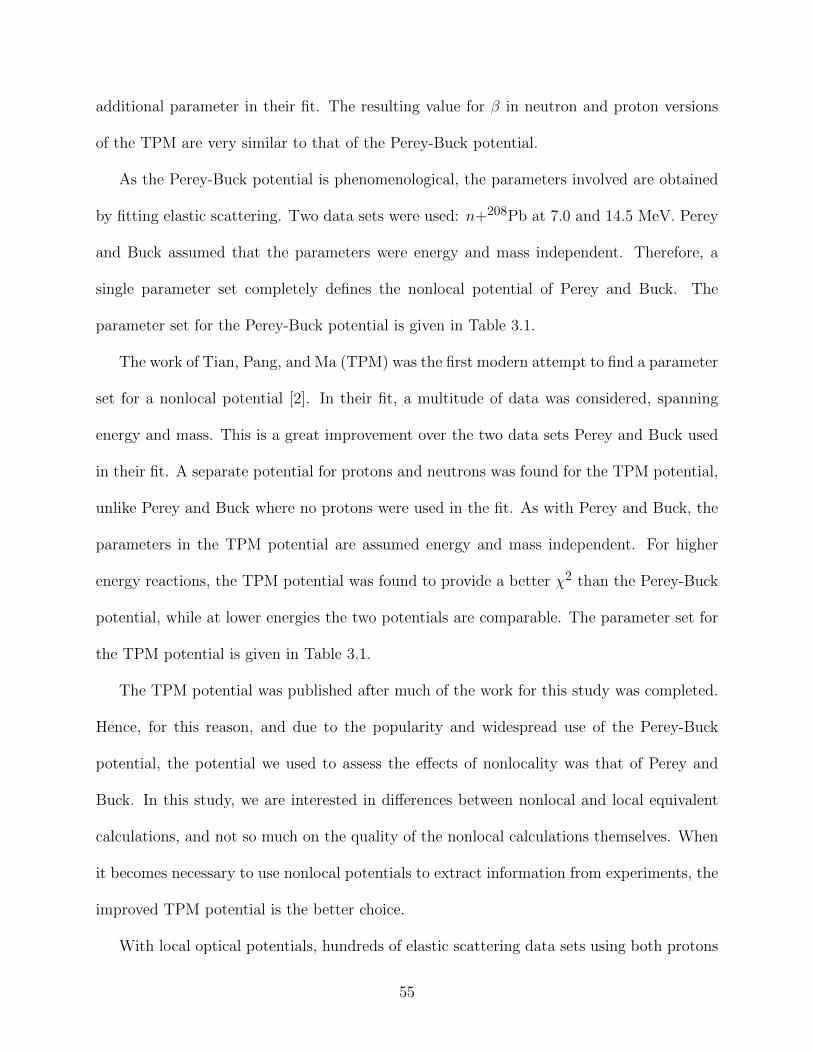
additional parameter in their fit. The resulting value for β in neutron and proton versions

of the TPM are very similar to that of the Perey-Buck potential.

As the Perey-Buck potential is phenomenological, the parameters involved are obtained

by fitting elastic scattering. Two data sets were used: n+208Pb at 7.0 and 14.5 MeV. Perey

and Buck assumed that the parameters were energy and mass independent. Therefore, a

single parameter set completely defines the nonlocal potential of Perey and Buck. The

parameter set for the Perey-Buck potential is given in Table 3.1.

The work of Tian, Pang, and Ma (TPM) was the first modern attempt to find a parameter

set for a nonlocal potential [2]. In their fit, a multitude of data was considered, spanning

energy and mass. This is a great improvement over the two data sets Perey and Buck used

in their fit. A separate potential for protons and neutrons was found for the TPM potential,

unlike Perey and Buck where no protons were used in the fit. As with Perey and Buck, the

parameters in the TPM potential are assumed energy and mass independent. For higher

energy reactions, the TPM potential was found to provide a better χ2 than the Perey-Buck

potential, while at lower energies the two potentials are comparable. The parameter set for

the TPM potential is given in Table 3.1.

The TPM potential was published after much of the work for this study was completed.

Hence, for this reason, and due to the popularity and widespread use of the Perey-Buck

potential, the potential we used to assess the effects of nonlocality was that of Perey and

Buck. In this study, we are interested in differences between nonlocal and local equivalent

calculations, and not so much on the quality of the nonlocal calculations themselves. When

it becomes necessary to use nonlocal potentials to extract information from experiments, the

improved TPM potential is the better choice.

With local optical potentials, hundreds of elastic scattering data sets using both protons

55

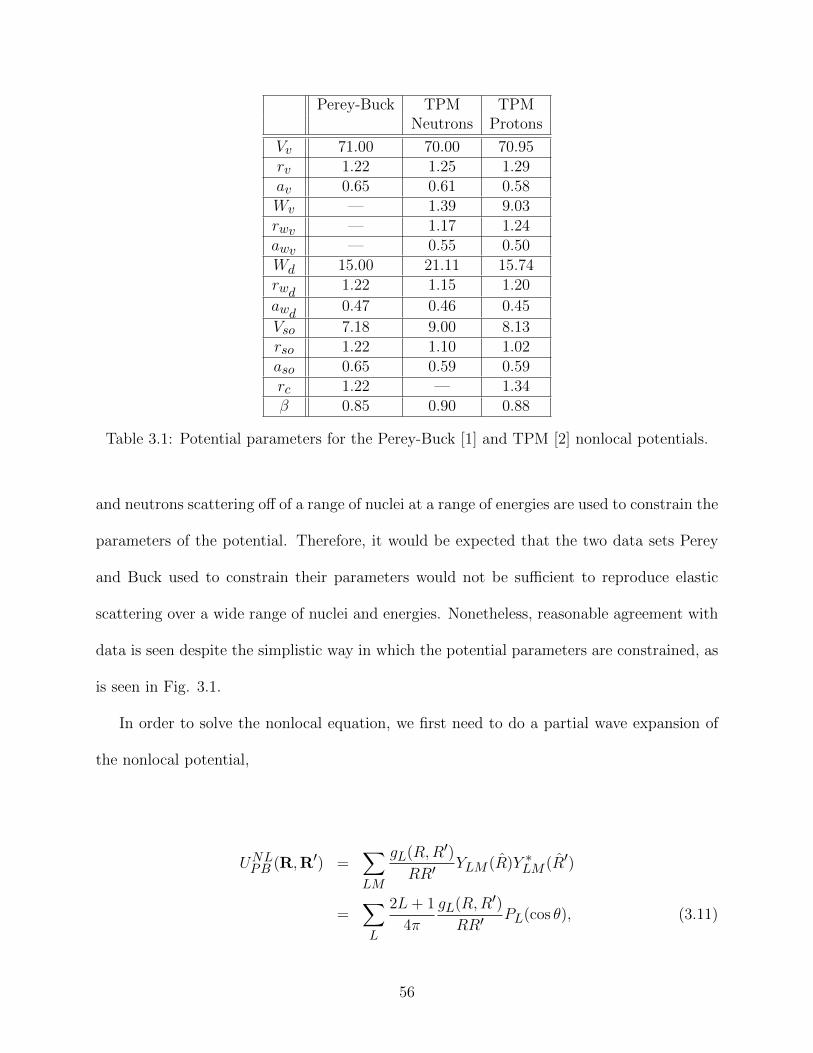
Perey-Buck TPM TPMNeutrons Protons

Vv 71.00 70.00 70.95rv 1.22 1.25 1.29av 0.65 0.61 0.58Wv — 1.39 9.03rwv — 1.17 1.24awv — 0.55 0.50Wd 15.00 21.11 15.74rwd 1.22 1.15 1.20

awd 0.47 0.46 0.45

Vso 7.18 9.00 8.13rso 1.22 1.10 1.02aso 0.65 0.59 0.59rc 1.22 — 1.34β 0.85 0.90 0.88

Table 3.1: Potential parameters for the Perey-Buck [1] and TPM [2] nonlocal potentials.

and neutrons scattering off of a range of nuclei at a range of energies are used to constrain the

parameters of the potential. Therefore, it would be expected that the two data sets Perey

and Buck used to constrain their parameters would not be sufficient to reproduce elastic

scattering over a wide range of nuclei and energies. Nonetheless, reasonable agreement with

data is seen despite the simplistic way in which the potential parameters are constrained, as

is seen in Fig. 3.1.

In order to solve the nonlocal equation, we first need to do a partial wave expansion of

the nonlocal potential,

UNLPB (R,R′) =∑LM

gL(R,R′)RR′

YLM (R)Y ∗LM (R′)

=∑L

2L+ 1

4π

gL(R,R′)RR′

PL(cos θ), (3.11)

56

0 30 60 90 120 150 180θ

c.m. [deg]

0.0

0.5

1.0

1.5

2.0

2.5

3.0

3.5

4.0σ/

σ RPerey-BuckData

a)

0 20 40 60 80 100 120θ

c.m. [deg]

0.00

0.25

0.50

0.75

1.00

1.25

1.50

1.75

2.00

σ/σ R

b)

Figure 3.1: Differential elastic scattering relative to Rutherford as a function of scatteringangle. (a) 48Ca(p, p)48Ca at 15.63 MeV with data from [9] (b) 208Pb(p, p)208Pb at 61.4 MeVwith data from [10].

where we defined θ as the angle between R and R′. Multiplying both sides by PL(cos θ),

integrating over all angles, using the orthogonality of the Legendre polynomials, and solving

for gL(R,R′), we find that

gL(R,R′) = 2πRR′∫ 1

−1UNLPB (R,R′)PL(cos θ)d(cos θ). (3.12)

Now, inserting the Perey-Buck form for the nonlocal potential, replacing 12

∣∣R + R′∣∣ with

12(R +R′), and doing a few lines of algebra outlined in Appendix A, we arrive at

gL(R,R′) =2iLz

π12β

jL(−iz)exp

(−R

2 +R′2

β2

)U

(1

2(R +R′)

)(3.13)

with z=2RR′β2

, and jL being spherical Bessel functions. We now have a partial wave equation

in terms of gL(R,R′) for each function χL(r):

~2

2µ

[d2

dr2− L(L+ 1)

R2

]χL(R) + EχL(R) =

∫gL(R,R′)χL(R′)dR′. (3.14)

57

3.3.1 Correction Factor

Ever since Perey and Buck introduced their potential in 1962, nearly all analytic work

involving approximations to nonlocal potentials, or corrections to wave functions due to a

nonlocal potential, assumed the Perey-Buck form for the nonlocality. That is, there is only

one nonlocality parameter, β, and the nonlocal part of the potential takes the form Eq.(3.9).

This is not true for the DOM or the Giannini-Ricco nonlocal potential, discussed later, where

there are several terms with a different nonlocality parameter.

Accounting for the nonlocality through the energy dependence of a local optical potential

is known to be insufficient. One key feature of a nonlocal potential is that it reduces the

amplitude of the wave function in the nuclear interior compared to the wave function from an

equivalent local potential. This is the so-called Perey effect [101]. Physically, the reduction of

the wave function can be understood to result from the repulsion due to the Pauli principle.

Since it wasn’t practical to solve the integro-differential equation with a nonlocal poten-

tial in the 1960s, there was great interest in finding a way to account for this reduction of

amplitude while still keeping the simplicity of solving a local equation. This was first accom-

plished by Austern, who studied the wave functions of nonlocal potentials and demonstrated

the Perey effect in one dimension [73]. Later, Fiedeldey did a similar study for the three

dimensional case [75]. Using a different method, Austern presented a way to relate wave

functions obtained from a nonlocal and a local potential in the three-dimensional case [74].

Since then, nonlocal calculations have been avoided using the Perey correction factor (PCF).

The Perey correction factor is derived in detail in Appendix B. Here we simply outline

the derivation. To derive the PCF, we begin with the three dimensional Schrodinger equation

58

~2

2µ∇2ΨNL(R) + EΨNL(R) = Uo(R)ΨNL(R) +

∫UNL(R,R′)ΨNL(R′)dR′, (3.15)

where Uo(R) is the local part of the potential, and typically contains spin-orbit and Coulomb

terms. Let us define a function, F (R) that connects the local wave function Ψloc(R) resulting

from the potential ULE(R) with the wave function resulting from a nonlocal potential,

ΨNL(R):

ΨNL(R) ≡ F (R)Ψloc(R). (3.16)

The potential ULE(R) is defined such that it reproduces the exact same elastic scattering

as the nonlocal potential. Since the local and nonlocal equations describe the same elastic

scattering, the wave functions should be identical outside the nuclear interior. Thus, F (R)→

1 as R→∞. The local equation that Ψloc satisfies is:

~2

2µ∇2Ψloc(R) + EΨloc(R) = ULE(R)Ψloc(R). (3.17)

Combining Eq.(3.15) and Eq.(3.17) with the assumption of Eq.(3.16) we obtain:

F (r) =

(1− µβ2

2~2[ULE(R)− Uo(R)

])−1/2. (3.18)

59

It should be noted that the PCF is only valid for nonlocal potentials of the Perey-Buck

form. However, there is no reason to expect that the full nonlocality in the optical potential

will look anything like the Perey-Buck form. On physical grounds, the optical potential

must be energy dependent due to nonlocalities arising from channel couplings. While the

specific form chosen for the Perey-Buck potential is convenient for numerical calculations, a

single Gaussian term mocking up all energy-independent nonlocal effects is likely to be an

oversimplification.

3.4 Giannini-Ricco Nonlocal Potential

The Perey-Buck potential remained the only widely known and used nonlocal potential

available for the following 15 years after its development. An attempt by Giannini and

Ricco was made to construct a nonlocal potential of a similar form but with more data

constraining the parameters [71, 72]. Their first work focused on N = Z spherical nuclei,

while their second work made an extension to N 6= Z nuclei. Unfortunately, in doing the

fits, no nonlocal calculations were performed. Instead, the fits were done using a purely local

optical potential, and a transformation formula was used which related nonlocal and local

form factors. This transformation formula is derived in Appendix B.

To construct their potential, Giannini and Ricco first derived a general expression of the

nonlocal potential in the framework of Watson multiple-scattering theory [55]. The form of

the derived nonlocal potential is a guide for the parametrization of the phenomenological

optical potential, whose parameter values are fitted to both elastic scattering and bound state

properties. To do the fit, a local form for the optical potential was chosen. The parameters

were varied to obtain a best fit of the available data, and then the transformation formulas

60

were used to get the nonlocal Giannini-Ricco potential for N = Z nuclei (GR76) [71], and

later for N 6= Z nuclei (GR80) [72]. We chose not to use this potential since the fits to data

were done using local potentials, and an unreliable transformation formula was used to get

the nonlocal potential.

3.5 Nonlocal Dispersive Optical Model Potential

An alternative method for obtaining the optical potential is through the self-energy, which

can be calculated microscopically using modern day structure theory. This is the method

by which the Dispersive Optical Model (DOM) is constructed. The DOM makes use of the

Kramers-Kronig dispersion relation that links the imaginary and real parts of the nucleon

self-energy [63, 65]. The optical potential is constrained by this dispersion relation. This

method was first introduced by Mahaux and Sartor [102]. The nuclear mean field is a function

of energy, where for E < 0 it is the shell-model potential that describes single-particle states,

while for E > 0 it is the optical model potential that describes scattering cross sections.

While the nuclear mean field is a continuous function of energy, its behavior as the energy

changes sign is not simple due to the coupling between elastic and inelastic channels. It is

this coupling that gives rise to the energy dependence and the imaginary component in the

optical potential. Through the dispersive relation, the scattering and bound state parts of

the nuclear mean field can be linked. The scattering parameters can be constrained by use of

fitting elastic scattering, and the bound state parameters can be constrained by comparisons

to single particle energies and (e, e′p) observables. As seen in Fig. 3.2, the nonlocal DOM

potential reproduces experimental elastic scattering data across a wide range of energies.

Using this dispersive relation, a local version of the DOM has been developed [103]. The

61

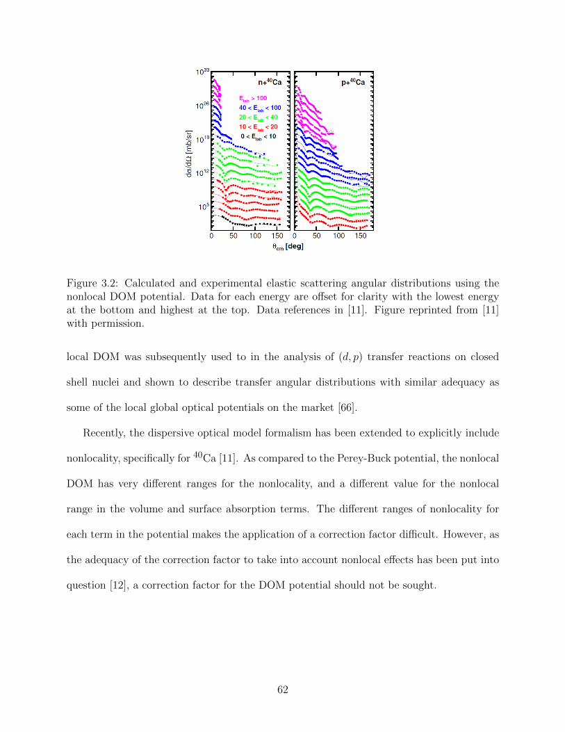
Figure 3.2: Calculated and experimental elastic scattering angular distributions using thenonlocal DOM potential. Data for each energy are offset for clarity with the lowest energyat the bottom and highest at the top. Data references in [11]. Figure reprinted from [11]with permission.

local DOM was subsequently used to in the analysis of (d, p) transfer reactions on closed

shell nuclei and shown to describe transfer angular distributions with similar adequacy as

some of the local global optical potentials on the market [66].

Recently, the dispersive optical model formalism has been extended to explicitly include

nonlocality, specifically for 40Ca [11]. As compared to the Perey-Buck potential, the nonlocal

DOM has very different ranges for the nonlocality, and a different value for the nonlocal

range in the volume and surface absorption terms. The different ranges of nonlocality for

each term in the potential makes the application of a correction factor difficult. However, as

the adequacy of the correction factor to take into account nonlocal effects has been put into

question [12], a correction factor for the DOM potential should not be sought.

62

3.6 Local Equivalent Potentials

To assess the effects of nonlocal potentials, a local phase equivalent (LPE) potential needs

to be found. A local potential is considered ’phase equivalent’ to a nonlocal potential if it

reproduces the same elastic scattering. This definition is chosen since optical potentials are

constructed through fits to elastic scattering data. Therefore, if two potentials are able to

generate the same elastic scattering distribution, then the two potentials are indistinguishable

at the level of elastic scattering, regardless of their form.

The downside of this definition is that the short-ranged nonlocal effects are not con-

strained through elastic scattering. To find a LPE potential, we first assume some form

for the LPE potential. This form is normally chosen to mimic the shape of the nonlocal

potential. As an example, the Perey-Buck nonlocal potential has real volume, real spin-

orbit, and imaginary surface terms. Therefore, the LPE potential was chosen to have the

same terms. We calculate the elastic scattering distribution generated from the nonlocal

potential, then vary the parameters of our LPE potential to obtain a best fit to the elastic

scattering distribution. This was done with the code SFRESCO [104] which performs a χ2

minimization.

Another method to obtain a LPE potential is through S-matrix inversion [105, 106].

This has the advantage over elastic scattering fits since the resulting potential will exactly

reproduce the S-matrix elements you started with [107]. However, it is important to note

that the S-matrix is not an observable, so one cannot extract an S-matrix for each partial

wave from elastic scattering data.

Exactly reproducing the S-matrix elements from the nonlocal calculation when doing the

local fit was one difficulty we encountered in this study. While the fits visually looked very

63

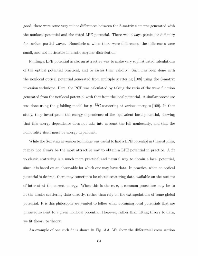
good, there were some very minor differences between the S-matrix elements generated with

the nonlocal potential and the fitted LPE potential. There was always particular difficulty

for surface partial waves. Nonetheless, when there were differences, the differences were

small, and not noticeable in elastic angular distribution.

Finding a LPE potential is also an attractive way to make very sophisticated calculations

of the optical potential practical, and to assess their validity. Such has been done with

the nonlocal optical potential generated from multiple scattering [108] using the S-matrix

inversion technique. Here, the PCF was calculated by taking the ratio of the wave function

generated from the nonlocal potential with that from the local potential. A similar procedure

was done using the g-folding model for p+12C scattering at various energies [109]. In that

study, they investigated the energy dependence of the equivalent local potential, showing

that this energy dependence does not take into account the full nonlocality, and that the

nonlocality itself must be energy dependent.

While the S-matrix inversion technique was useful to find a LPE potential in these studies,

it may not always be the most attractive way to obtain a LPE potential in practice. A fit

to elastic scattering is a much more practical and natural way to obtain a local potential,

since it is based on an observable for which one may have data. In practice, when an optical

potential is desired, there may sometimes be elastic scattering data available on the nucleus

of interest at the correct energy. When this is the case, a common procedure may be to

fit the elastic scattering data directly, rather than rely on the extrapolations of some global

potential. It is this philosophy we wanted to follow when obtaining local potentials that are

phase equivalent to a given nonlocal potential. However, rather than fitting theory to data,

we fit theory to theory.

An example of one such fit is shown in Fig. 3.3. We show the differential cross section

64

over the Rutherford cross section as a function of the scattering angle. The solid line is the

elastic scattering distribution generated using the Perey-Buck nonlocal potential. The open

circles are a fit to the nonlocal solution, and the dotted line is obtained by transforming the

depths of the volume and surface potentials [12]. Notice that the local fit is essentially exact

all the way out to 180. The transformation formulas relied on by Giannini and Ricco to

construct their potential represents the dotted line. The inadequacy of the transformation

formula to reproduce the solution with the nonlocal potential is why the Giannini-Ricco

potential was not favored in this study.

0 20 40 60 80 100 120 140 160 180θ

c.m. (deg)

1

10

σ/σ R

uth

Perey-BuckLocal FitTransformed Depths

Figure 3.3: 49Ca(p, p)49Ca at 50.0 MeV: The solid line is obtained from using the Perey-Bucknonlocal potential, the open circles are a fit to the nonlocal solution, and the dotted line isobtained by transforming the depths of the volume and surface potentials according to Eq.(B.14). Figure reprinted from [12] with permission.

65

Chapter 4

Results

For many years nonlocality has been effectively included in calculations by use of the Perey

correction factor (PCF) [73, 75], as discussed in Sec. 3.3.1. However, the PCF is only

suitable for use with potentials of the Perey-Buck form, and thus not of use for the DOM

potential or a microscopically derived optical potential. In addition, the quality of the PCF

has never been rigorously tested. Therefore, the first part of this study was to investigate

if the correction factor was adequately able to account for the impact of nonlocality on the

wave functions.

The reduction of the wave function can be understood physically in terms of the repulsion

between fermions due to the Pauli principle. Since one major source of nonlocality is due

to anti-symmetrization, this repulsion will naturally have the effect of pushing some of the

wave function out of the interior as compared to an interaction that doesn’t take anti-

symmetrization into account.

The deuteron scattering state is also affected by nonlocality. When using the DWBA, it

is possible to apply a correction factor to the deuteron scattering wave function. However, a

nonlocal global deuteron optical potential does not exist for the purpose of comparison. Also,

as we have discussed, the DWBA does not take deuteron breakup into account explicitly.

Therefore, we would like to use the more advanced ADWA which does consider breakup, and

relies on better constrained nucleon optical potentials, of which nonlocal global potentials

exist (i.e. Perey-Buck).

66

The numerical details of the calculations performed in this thesis are presented in Sec.

4.1. The results of this thesis will be presented in three parts. The first part in Sec.

4.2 investigates (p, d) transfer reactions on 17O, 41Ca, 49Ca, 127Sn, 133Sn, and 209Pb at

proton energies of Ep = 20 and 50 MeV. The transfer cross sections were calculated within

the DWBA, and nonlocality in the deuteron channel is not included. In this study, we

investigated the effect of nonlocality on the proton scattering wave function and the neutron

bound state wave function. We also examined the validity of the commonly used PCF to

effectively include nonlocality.

Next, in Sec. 4.3, we studied (p, d) transfer reactions on 40Ca at proton energies of

Ep = 20, 35, and 50 MeV using the nonlocal DOM potential, as well as the Perey-Buck

potential. Once again, the transfer cross section was calculated within the DWBA, and

nonlocality in the deuteron channel is not included. Here we studied hole states rather

than single particle states, as in the previous study. Hence, the goal of this study was to

understand if the effects of nonlocality seen in the previous study could be generalized to

hole states, and to see if the same conclusions can be drawn when using a different form for

the nonlocal potential.

Finally, in Sec. 4.4, we studied (d, p) reactions on 16O, 40Ca, 48Ca, 126Sn, 132Sn, and

208Pb at deuteron energies of Ed = 10, 20 and 50 MeV. For these cases, nonlocality was

included explicitly in the deuteron scattering state within the ADWA, as well as in the

proton channel. In all wave functions, the Perey-Buck nonlocal potential was used. This

study sought to quantify the effect of nonlocality when included consistently in calculations

of single nucleon transfer reactions including deuteron breakup.

It is important to note that the purpose of this work is not to describe the data. We do not

expect that the Perey-Buck potential, developed in the sixties for n+208Pb at intermediate

67

energies using two data sets, will do well for a wide range of targets and energies. The

focus should be on the differences between the nonlocal and the local calculations under

the constraint of the same physical input, namely, that both the nonlocal and local optical

potentials introduced reproduce the exact same elastic scattering.

4.1 Numerical Details

To compare the results of the nonlocal calculations, we must compare our results to calcu-

lations using local potentials with the same constraints. Therefore, to constrain the local

nucleon-target optical potentials, we require that they reproduce the same elastic scattering

obtained when using the Perey-Buck or the DOM potential at the relevant energies. For the

proton scattering states, we calculate (p, p) elastic scattering at the relevant energy using the

Perey-Buck or DOM potential, then fit the resulting distribution to a local form. The fitting

of these local phase equivalent (LPE) potentials was performed using the code SFRESCO

[104].

For the deuteron scattering states, the procedure is somewhat different. In Secs. 4.2

and 4.3 we use the local global deuteron optical potential of Daehnick [84] evaluated at the

relevant energy. In Sec. 4.4, we calculate (n, n) and (p, p) elastic scattering at half the

deuteron energy using the Perey-Buck potential, and again found LPE potentials for the

elastic scattering distributions. The local adiabatic potential is then calculated with the

proton and neutron LPE potentials.

For the neutron bound states, we calculated the nonlocal equation using a real Woods-

Saxon form with a nonlocality range of β = 0.85 fm. We also used a local spin-orbit

interaction with a depth fixed at 6 MeV. For each term we used a radius of r = 1.25 fm

68

and a = 0.65 fm. The depth of the nonlocal real Woods-Saxon form was then adjusted to

reproduce the physical binding energy. Also, in Sec. 4.3 we used the nonlocal DOM potential

to calculate the neutron bound state. The corresponding bound state resulting from local

potentials was obtained by setting β = 0 and adjusting the local real Woods-Saxon depth to

reproduce the binding energy.

In Secs. 4.2 and 4.3, the calculated wave functions were read into the code FRESCO to

calculate the (p, d) transfer cross sections. We used the Reid soft core interaction [110] in

the (p, d) T-matrix and to calculate the deuteron bound state. In Sec. 4.4, the bound and

scattering states that are calculated are inserted into the (d, p) T-matrix Eq.(2.21). This

was implemented in the code NLAT (NonLocal Adiabatic Transfer). The NN interaction

in this case was a central Gaussian which reproduces the binding energy and radius of the

deuteron ground state, as in [96].

In Secs. 4.2 and 4.3 the scattering wave functions were solved by using a 0.05 fm radial

step size with a matching radius of 40 fm. For the bound states solutions, we used a

radial step size of 0.02 fm. The matching radius was half the radius of the nucleus under

consideration, and the maximum radius was 30 fm. The cross sections contain contributions

of partial waves up to J = 30.

In Sec. 4.4 the scattering wave functions were calculated in steps of 0.01 fm with a

matching radius of 30 fm. The nonlocal adiabatic potential was obtained on a radial grid of

step 0.05 fm. We used linear interpolation to calculate the nonlocal adiabatic potential in

steps of 0.01 fm in order to calculate the adiabatic deuteron wave function with the same

step size. The bound state wave functions were also calculated in steps of 0.01 fm with a

maximum radius of 30 fm and a matching radius of half the radius of the nucleus under

consideration. Again, converged cross sections contain partial waves up to J = 30.

69

16O(d, p) 40Ca(d, p) 48Ca(d, p) 126Sn(d, p) 132Sn(d, p) 208Pb(d, p)

10 MeV −1.92% −2.69% −0.39% 0.32% 0.73% 1.48%20 MeV −1.87% −2.26% −0.34% −0.65% 0.17% 0.11%50 MeV −5.57% 0.07% −2.59% −0.41% −0.08% −0.38%

Table 4.1: Percent difference of the (d, p) transfer cross section at the first peak for a calcu-lation including the remnant term relative to a calculation without the remnant term.

4.1.1 Effects of Neglecting Remnant

To get an idea of the significance of the remnant term, we show in Table 4.1 the percent

difference at the first peak of the (d, p) transfer cross section for a calculation with the

remnant term relative to a calculation without the remnant term for a wide range of targets.

These DWBA calculations used the deuteron global optical potential of Daehnick [84] to

describe the deuteron scattering state, and the LPE potentials to the Perey-Buck potential

for the proton scattering state, a central Gaussian for the deuteron bound state, and a real

Woods-Saxon form for the neutron bound state that reproduces the experimental binding

energy.

4.2 Distorted Wave Born Approximation with the Perey-

Buck Potential

The first part of this study was to investigate the effect of the Perey-Buck potential on the

entrance channel of (p, d) transfer reactions. For this study, nonlocality was included explic-

itly in the proton scattering state and the neutron bound state. Using the wave functions

generated with the nonlocal potentials, (p, d) transfer reactions were calculated. These cross

sections were compared to those generated with LPE potentials, discussed in Sec. 3.6. Also,

70

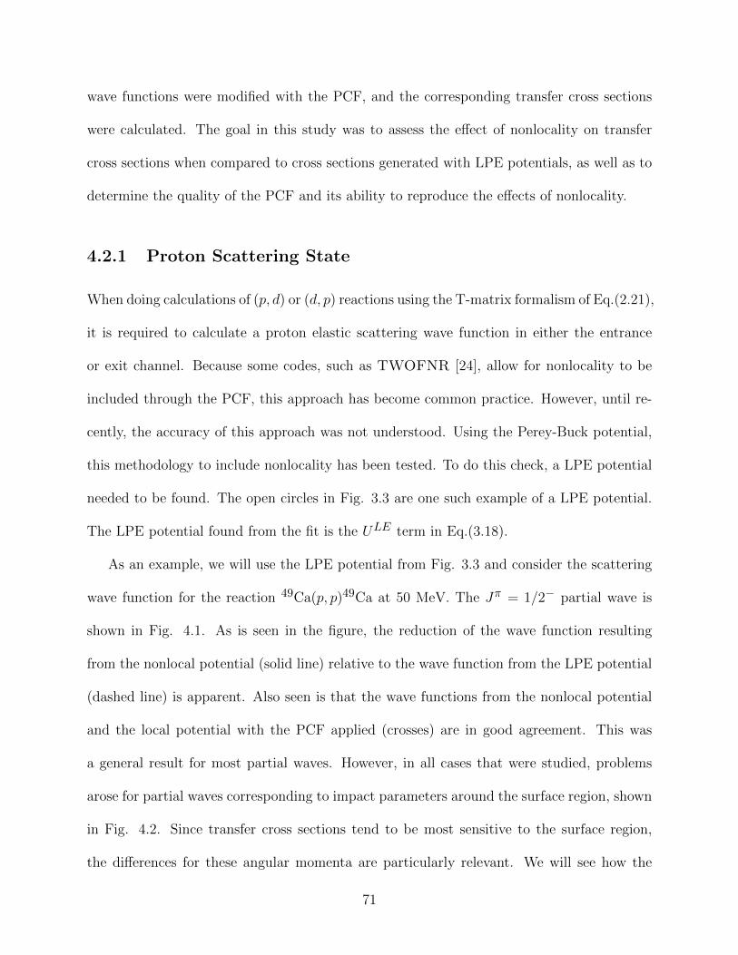
wave functions were modified with the PCF, and the corresponding transfer cross sections

were calculated. The goal in this study was to assess the effect of nonlocality on transfer

cross sections when compared to cross sections generated with LPE potentials, as well as to

determine the quality of the PCF and its ability to reproduce the effects of nonlocality.

4.2.1 Proton Scattering State

When doing calculations of (p, d) or (d, p) reactions using the T-matrix formalism of Eq.(2.21),

it is required to calculate a proton elastic scattering wave function in either the entrance

or exit channel. Because some codes, such as TWOFNR [24], allow for nonlocality to be

included through the PCF, this approach has become common practice. However, until re-

cently, the accuracy of this approach was not understood. Using the Perey-Buck potential,

this methodology to include nonlocality has been tested. To do this check, a LPE potential

needed to be found. The open circles in Fig. 3.3 are one such example of a LPE potential.

The LPE potential found from the fit is the ULE term in Eq.(3.18).

As an example, we will use the LPE potential from Fig. 3.3 and consider the scattering

wave function for the reaction 49Ca(p, p)49Ca at 50 MeV. The Jπ = 1/2− partial wave is

shown in Fig. 4.1. As is seen in the figure, the reduction of the wave function resulting

from the nonlocal potential (solid line) relative to the wave function from the LPE potential

(dashed line) is apparent. Also seen is that the wave functions from the nonlocal potential

and the local potential with the PCF applied (crosses) are in good agreement. This was

a general result for most partial waves. However, in all cases that were studied, problems

arose for partial waves corresponding to impact parameters around the surface region, shown

in Fig. 4.2. Since transfer cross sections tend to be most sensitive to the surface region,

the differences for these angular momenta are particularly relevant. We will see how the

71

0 1 2 3 4 5 6 7 8 9 10 11 12 13 14 15r [fm]

-0.4

-0.2

0

0.2

0.4

0.6

0.8

ψ(r

) [f

m-1

/2]

-|Im

(ψ)|

|R

e(ψ

)|

NonlocalCorrected LocalUncorrected Local

Figure 4.1: Real and imaginary parts of the Jπ = 1/2− partial wave of the scattering wavefunction for the reaction 49Ca(p, p)49Ca at 50.0 MeV: ψNL (solid line), ψPCF (crosses), andψloc (dashed line). Top (bottom) panel: absolute value of the real (imaginary) part of thescattering wave function. Figure reprinted from [12] with permission.

inadequacy of the PCF for surface partial wave affects the resulting transfer cross sections

in Sec. 4.2.3.

0 1 2 3 4 5 6 7 8 9 10 11 12 13 14 15r [fm]

-0.6

-0.4

-0.2

0

0.2

0.4

0.6

0.8

ψ(r

) [f

m-1

/2]

-|Im

(ψ)|

|R

e(ψ

)|

NonlocalCorrected LocalUncorrected Local

Figure 4.2: Real and imaginary parts of the Jπ = 11/2+ partial wave of the scatteringwave function for the reaction 49Ca(p, p)49Ca at 50.0 MeV. See caption of Fig. 4.1. Figurereprinted from [12] with permission.

72

This inability of the PCF to correct surface partial waves is partly due to the way in which

it was derived. When deriving the PCF, terms related to ∇2F were neglected, such as the

one in Eq.(B.21). This term only contributes around the nuclear surface. In addition, when

performing the local fit, we occasionally found slight differences in the S-matrix elements for

a particular partial wave. Since the scattering wave functions are normalized according to

Eq.(2.2), these small changes in the S-matrix will result in different amplitudes for the real

and imaginary parts of the scattering wave function in the asymptotic region.

4.2.2 Neutron Bound State

We now turn our attention to the neutron bound state that exists in the entrance channel

of (p, d) reactions. In order to investigate the effects of nonlocality on the bound state wave

functions, and the adequacy of the PCF to correct for nonlocality, the PCF was applied to

the local bound state wave function, and the resulting wave function was renormalized to

unity.

To illustrate, the 2p3/2 ground state wave function for n+48Ca is shown in Fig. 4.3.

Visually, the correction factor does an excellent job correcting for nonlocality in the bound

state. However, it is important to notice that in the surface region (2 − 5 fm), the PCF

does very little to bring the wave function resulting from the local equivalent potential into

agreement with the wave function resulting from the nonlocal potential. The inset, which

shows the difference between φNL and φPCF , emphasizes this fact.

As stated in Sec. 4.2.1, the reason for the inadequacy of the PCF in the surface region

goes back to the way in which the PCF was derived. In this case, the bound wave function

has a large slope around the surface resulting in large differences between the wave function

generated using nonlocal interactions and the one generated from local interactions.

73

0 1 2 3 4 5 6 7 8 9 10r [fm]

−0.6

−0.4

−0.2

0

0.2

0.4

φ(r)

[fm

-1/2

]

NonlocalCorrected LocalUncorrected Local

0 1 2 3 4 5 6 7 8 9 10r [fm]

-0.02

0.00

0.02

0.04

0.06

φ NL-

φ PC

F [fm

-1/2

]

Figure 4.3: Ground state, 2p3/2, bound wave function for n+48Ca. φNL (solid line), φPCF

(crosses), and φloc (dashed line). The inset shows the difference φNL − φPCF . Figurereprinted from from [12] with permission.

Another important point to note is that nonlocality has the effect of increasing the

normalization of the asymptotic properties of the wave function (the ANC). Since nonlocality

reduces the amplitude of the wave function in the nuclear interior, and the wave function is

always normalized to unity, the ANC must increase. Therefore, the ANC of the bound wave

function resulting from nonlocal potentials was found to always be larger than the ANC from

local potentials, and the ANC of the corrected wave function was somewhere in between.

4.2.3 (p, d) Transfer Cross Sections - Distorted Wave Born Ap-

proximation

Now that we have studied the effect of nonlocality on the scattering and bound state wave

functions, we can investigate the effect nonlocality has on (p, d) transfer reactions when

74

nonlocality is included explicitly in the entrance channel.

As a first example, consider the transfer reaction corresponding to the wave functions we

have been studying in Secs. 4.2.1 and 4.2.2, 49Ca(p, d)48Ca at a proton energy of Ep = 50

MeV in the laboratory frame. The separate and combined effects of nonlocality in the bound

and scattering states are shown in Fig. 4.4. The solid line corresponds to when nonlocality

is included in both the proton scattering state and the neutron bound state, the dashed

line corresponds to the distribution obtained when only local equivalent potentials are used,

the crosses correspond to the cross section obtained when the proton scattering state and

neutron bound state wave functions are both corrected with the PCF. Also shown with the

dotted line is the cross section when nonlocality was only added to the scattering state, and

the dot-dashed line when nonlocality is only added to the neutron bound state.

0 5 10 15 20 25 30 35 40 45 50θ

c.m. (deg)

0.0

0.5

1.0

1.5

2.0

2.5

3.0

3.5

4.0

4.5

5.0

dσ/d

Ω [

mb/

sr]

NonlocalCorrected LocalUncorrected LocalNonlocal Scattering StateNonlocal Bound State

Figure 4.4: Angular distributions for 49Ca(p, d)48Ca at 50 MeV: Inclusion of nonlocality inboth the proton scattering state and the neutron bound state (solid), using LPE potentials,then applying the correction factor to both the scattering and bound states (crosses), usingthe LPE potentials without applying any corrections (dashed line), including nonlocality onlyin the proton scattering state (dotted line) and including nonlocality only in the neutronbound state (dot-dashed line). Figure reprinted from [12] with permission.

75

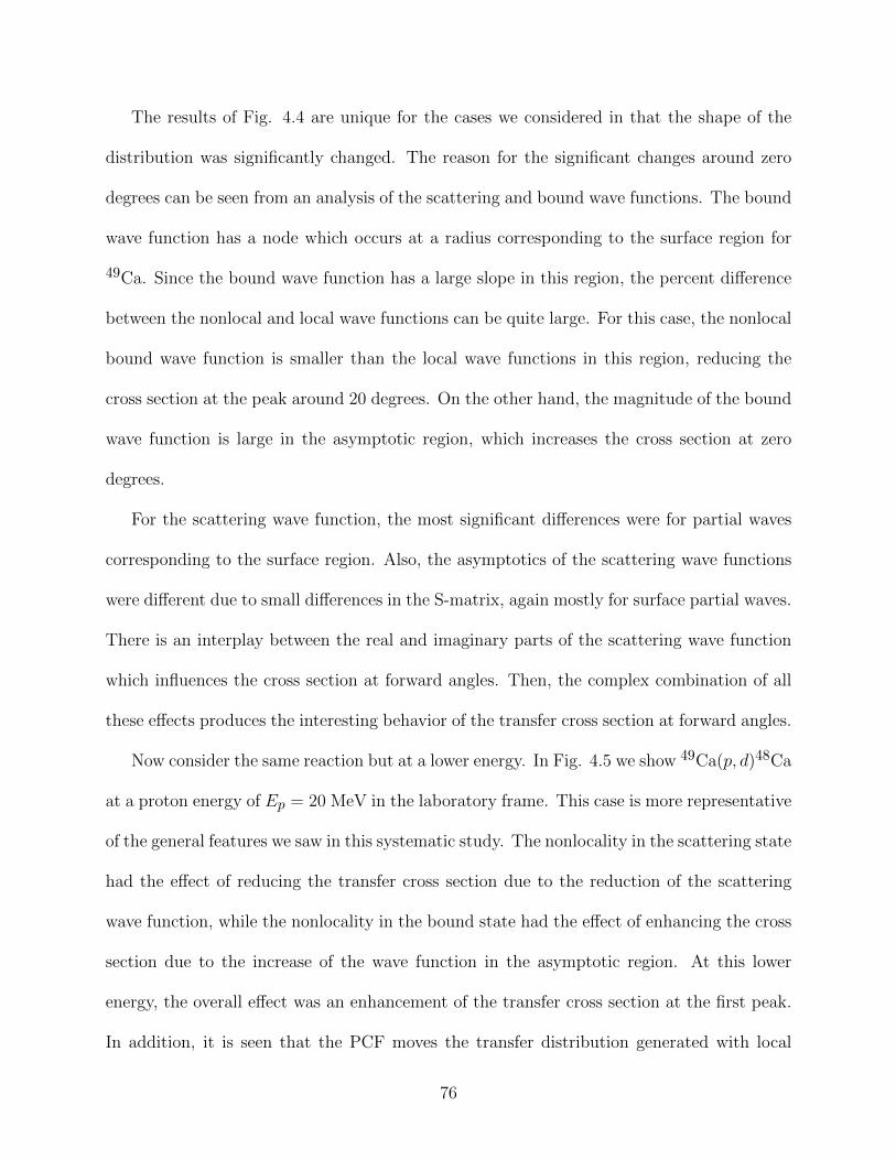
The results of Fig. 4.4 are unique for the cases we considered in that the shape of the

distribution was significantly changed. The reason for the significant changes around zero

degrees can be seen from an analysis of the scattering and bound wave functions. The bound

wave function has a node which occurs at a radius corresponding to the surface region for

49Ca. Since the bound wave function has a large slope in this region, the percent difference

between the nonlocal and local wave functions can be quite large. For this case, the nonlocal

bound wave function is smaller than the local wave functions in this region, reducing the

cross section at the peak around 20 degrees. On the other hand, the magnitude of the bound

wave function is large in the asymptotic region, which increases the cross section at zero

degrees.

For the scattering wave function, the most significant differences were for partial waves

corresponding to the surface region. Also, the asymptotics of the scattering wave functions

were different due to small differences in the S-matrix, again mostly for surface partial waves.

There is an interplay between the real and imaginary parts of the scattering wave function

which influences the cross section at forward angles. Then, the complex combination of all

these effects produces the interesting behavior of the transfer cross section at forward angles.

Now consider the same reaction but at a lower energy. In Fig. 4.5 we show 49Ca(p, d)48Ca

at a proton energy of Ep = 20 MeV in the laboratory frame. This case is more representative

of the general features we saw in this systematic study. The nonlocality in the scattering state

had the effect of reducing the transfer cross section due to the reduction of the scattering

wave function, while the nonlocality in the bound state had the effect of enhancing the cross

section due to the increase of the wave function in the asymptotic region. At this lower

energy, the overall effect was an enhancement of the transfer cross section at the first peak.

In addition, it is seen that the PCF moves the transfer distribution generated with local

76

0 5 10 15 20 25 30 35 40 45 50θ

c.m. (deg)

05

10152025303540455055

dσ/d

Ω [m

b/sr

]

NonlocalCorrected LocalUncorrected LocalNonlocal Scattering StateNonlocal Bound State

Figure 4.5: Same as in Fig. 4.4 but for 49Ca(p, d)48Ca at Ep = 20 MeV. Figure reprintedfrom [12] with permission.

0 5 10 15 20 25 30 35 40 45 50θ

c.m. (deg)

0

2

4

6

8

10

12

14

dσ/d

Ω [m

b/sr

]

NonlocalCorrected LocalUncorrected LocalNonlocal Scattering StateNonlocal Bound State

Figure 4.6: Same as in Fig. 4.4 but for 133Sn(p, d)132Sn at Ep = 20 MeV. Figure reprintedfrom [12] with permission.

potentials in the direction of that generated with nonlocal potentials. However, the PCF

was not able to fully take the effects of nonlocality into account.

Next we consider heavier targets, such as 133Sn and 209Pb, at Ep = 20 MeV. In both of

these cases the inclusion of nonlocality in the scattering state decreased the cross section by

77

0 10 20 30 40 50 60 70 80 90θ

c.m. (deg)

0.0

0.4

0.8

1.2

1.6

2.0

dθ/d

Ω [m

b/sr

]

NonlocalCorrected LocalUncorrected LocalNonlocal Scattering StateNonlocal Bound State

Figure 4.7: Same as in Fig. 4.4 but for 209Pb(p, d)208Pb at Ep = 20 MeV. Figure reprintedfrom [12] with permission.

a smaller amount than was seen before. This is due to the low energy of the proton and the

high charge of the target. Nonlocality in the proton scattering state reduced the magnitude

of the wave function in the nuclear interior, but the energy of the proton was not high enough

to penetrate deeply due to the large Coulomb barrier. On the other hand, nonlocality in the

bound state is very significant. Since the projectile energy was low, and the charge of the

target was high, the reaction is dominated by the asymptotitcs of the bound wave function,

which is enhanced in the nonlocal case.

For 133Sn(p, d)132Sn at Ep = 20 MeV, Fig. 4.6, the PCF does a reasonable job tak-

ing nonlocality into account, but there are still discrepancies between the full nonlocal and

corrected local solutions. For 209Pb(p, d)208Pb at Ep = 20 MeV, Fig. 4.7, there are discrep-

ancies at forward angles, but the distributions resulting from nonlocal and local potentials

coincidentally agree at the peak. This agreement is accidental, and comes from the nonlocal

effect in the bound state canceling that in the scattering state.

78

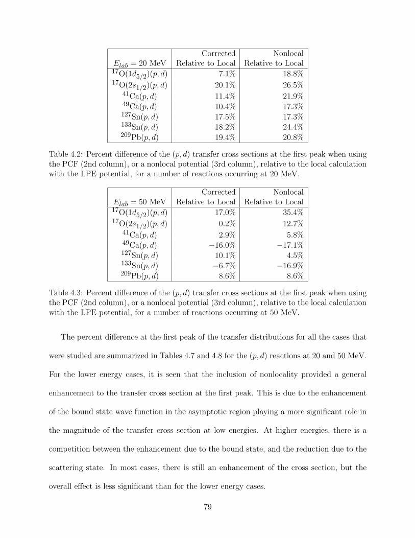
Corrected NonlocalElab = 20 MeV Relative to Local Relative to Local17O(1d5/2)(p, d) 7.1% 18.8%17O(2s1/2)(p, d) 20.1% 26.5%

41Ca(p, d) 11.4% 21.9%49Ca(p, d) 10.4% 17.3%127Sn(p, d) 17.5% 17.3%133Sn(p, d) 18.2% 24.4%209Pb(p, d) 19.4% 20.8%

Table 4.2: Percent difference of the (p, d) transfer cross sections at the first peak when usingthe PCF (2nd column), or a nonlocal potential (3rd column), relative to the local calculationwith the LPE potential, for a number of reactions occurring at 20 MeV.

Corrected NonlocalElab = 50 MeV Relative to Local Relative to Local17O(1d5/2)(p, d) 17.0% 35.4%17O(2s1/2)(p, d) 0.2% 12.7%

41Ca(p, d) 2.9% 5.8%49Ca(p, d) −16.0% −17.1%127Sn(p, d) 10.1% 4.5%133Sn(p, d) −6.7% −16.9%209Pb(p, d) 8.6% 8.6%

Table 4.3: Percent difference of the (p, d) transfer cross sections at the first peak when usingthe PCF (2nd column), or a nonlocal potential (3rd column), relative to the local calculationwith the LPE potential, for a number of reactions occurring at 50 MeV.

The percent difference at the first peak of the transfer distributions for all the cases that

were studied are summarized in Tables 4.7 and 4.8 for the (p, d) reactions at 20 and 50 MeV.

For the lower energy cases, it is seen that the inclusion of nonlocality provided a general

enhancement to the transfer cross section at the first peak. This is due to the enhancement

of the bound state wave function in the asymptotic region playing a more significant role in

the magnitude of the transfer cross section at low energies. At higher energies, there is a

competition between the enhancement due to the bound state, and the reduction due to the

scattering state. In most cases, there is still an enhancement of the cross section, but the

overall effect is less significant than for the lower energy cases.

79

4.2.4 Summary

In this study, the long established Perey correction factor (PCF) and the effects of nonlocal-

ity on the entrance channel of (p, d) reactions were studied. The integro-differential equation

containing the Perey-Buck nonlocal potential was solved numerically for single channel scat-

tering and bound states. A local phase equivalent (LPE) potential was obtained by fitting

the elastic distribution generated by the Perey-Buck potential. The PCF was applied to the

wave functions generated with the LPE potentials or the local equivalent binding potentials,

and the scattering and bound state wave functions were then used in a finite-range DWBA

calculation in order to obtain (p, d) transfer cross sections.

We found that the explicit inclusion of nonlocality in the entrance channel increased the

transfer distribution at the first peak by 15− 35%. In most cases, the transfer distribution

from using a nonlocal potential increased relative to the distribution from the local potential.

In all cases, the PCF moved the transfer distribution in the direction of the distribution which

included nonlocality explicitly. However, nonlocality was never fully taken into account with

the PCF. The PCF can be improved by including the surface terms that were neglected, and

not assuming that the local momentum approximation is valid. Such additional corrections

were not pursued since the full nonlocal solution can be calculated.

4.3 Distorted Wave Born Approximation with the Dis-

persive Optical Model Potential

The results of the previous work by Titus and Nunes [12], covered in Sec. 4.2, demonstrated

that nonlocality is significant in the study of transfer reactions, and that the PCF is not

80

able to fully reproduce the complex effects of nonlocality. However, the previous study only

considered the Perey-Buck nonlocal potential. Recently, the nonlocal DOM potential for

40Ca was developed [11]. We wanted to see if nonlocality remains an important ingredient to

transfer reactions when a different nonlocal potential is used. Since the DOM was constructed

only for 40Ca, we were only able to consider 40Ca(p, d)39Ca reactions. For this study, we

investigated laboratory proton energies of Ep = 20, 35, and 50 MeV.

0 30 60 90 120 150 180θ

c.m. [deg]

0.01

0.1

1

10

σ/σ R

uth

DOMDOM LPEPBPB LPEData (19.57 MeV)

Figure 4.8: Angular distributions for elastic scattering normalized to Rutherford for protonson 40Ca at Ep = 20 MeV. The elastic scattering with the DOM potential (solid line), theDOM LPE potential (open circles), the Perey-Buck interaction (dashed line), and the Perey-Buck LPE potential (open squares). The data (closed diamonds) from [13]. Figure reprintedfrom [14] with permission.

4.3.1 Proton Scattering State

In investigating the effect of nonlocality when using the DOM potential, we no longer con-

sidered the PCF since there is no easy generalization of the PCF to the DOM potential.

This is because each term of the DOM potential has a different value for the nonlocality

parameter, β. While it would be possible to construct a PCF for the DOM potential, the

81

0 30 60 90 120 150 180θ

c.m. [deg]

0.01

0.1

1

10

σ/σ R

uth

DOMDOM LPEPBPB LPEData (51.93 MeV)

Figure 4.9: Same as in Fig. 4.8 but for Ep = 50 MeV. Data from [15]. Figure reprinted from[14] with permission.

results of the previous work by Titus and Nunes [12] made pursuing a PCF for the DOM

potential irrelevant.

In Figs. 4.8 and 4.9 we show the elastic distributions generated from the DOM and the

Perey-Buck nonlocal potentials along with the corresponding LPE potentials. We also show

the corresponding elastic scattering data at the closest relevant energy. It is seen from the

distributions that the DOM potential is superior when it comes to describing the data. This

should not be a surprise as the DOM potential was constructed from fits to nucleon elastic

scattering data on 40Ca while the Perey-Buck potential was constructed from neutron elastic

scattering on 208Pb at low energy. Nonetheless, the Perey-Buck potential does a reasonably

good job at describing the elastic scattering data for the energy and angular range that the

data is available.

To investigate the scattering wave functions, we consider the Jπ = 1/2+ partial wave

for scattering at Ep = 50 MeV in Fig. 4.10. For both the DOM and the Perey-Buck

82

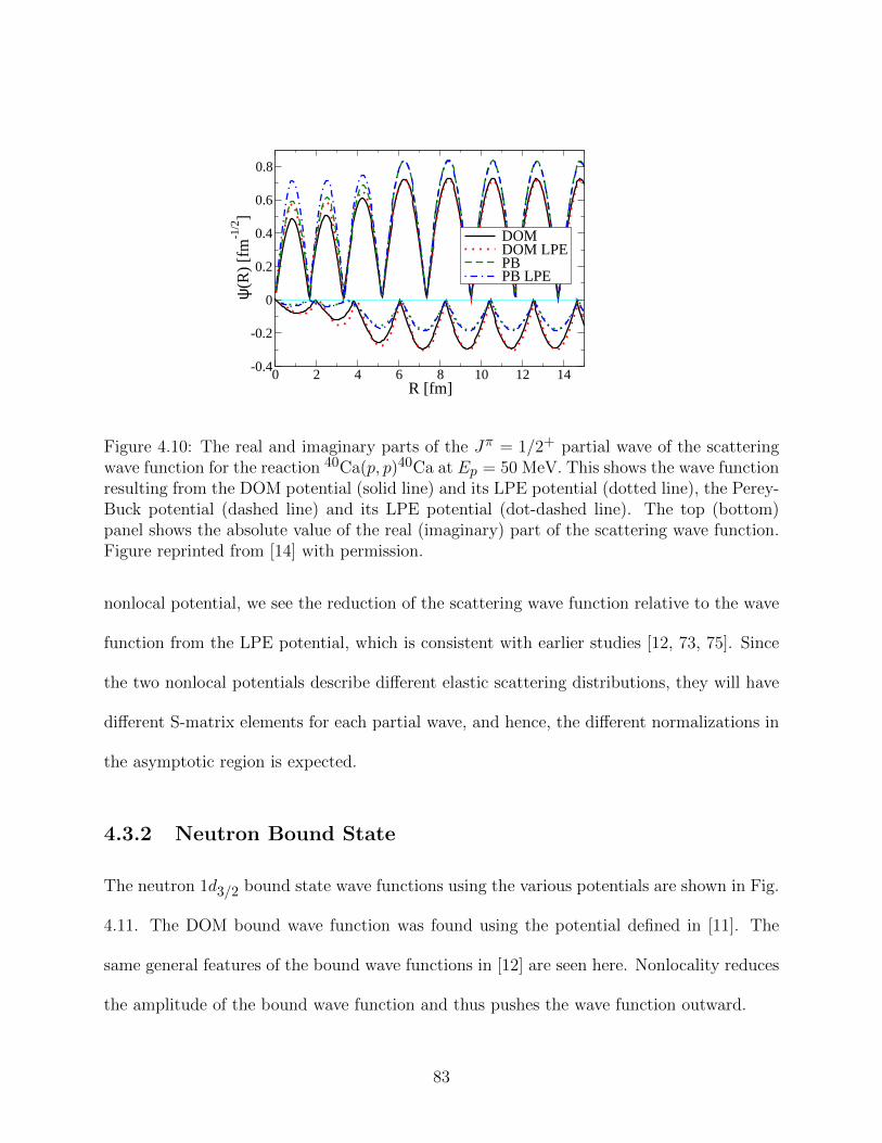
0 2 4 6 8 10 12 14R [fm]

-0.4

-0.2

0

0.2

0.4

0.6

0.8

ψ(R

) [f

m-1

/2]

DOMDOM LPEPBPB LPE

Figure 4.10: The real and imaginary parts of the Jπ = 1/2+ partial wave of the scatteringwave function for the reaction 40Ca(p, p)40Ca at Ep = 50 MeV. This shows the wave functionresulting from the DOM potential (solid line) and its LPE potential (dotted line), the Perey-Buck potential (dashed line) and its LPE potential (dot-dashed line). The top (bottom)panel shows the absolute value of the real (imaginary) part of the scattering wave function.Figure reprinted from [14] with permission.

nonlocal potential, we see the reduction of the scattering wave function relative to the wave

function from the LPE potential, which is consistent with earlier studies [12, 73, 75]. Since

the two nonlocal potentials describe different elastic scattering distributions, they will have

different S-matrix elements for each partial wave, and hence, the different normalizations in

the asymptotic region is expected.

4.3.2 Neutron Bound State

The neutron 1d3/2 bound state wave functions using the various potentials are shown in Fig.

4.11. The DOM bound wave function was found using the potential defined in [11]. The

same general features of the bound wave functions in [12] are seen here. Nonlocality reduces

the amplitude of the bound wave function and thus pushes the wave function outward.

83

0 1 2 3 4 5 6 7 8 9 10r [fm]

0

0.1

0.2

0.3

0.4

0.5

0.6

φ(r)

[fm

-1/2

]

DOMPBLocal

0 4 8 12r [fm]

0.01

0.1

φ(r)

[fm

-1/2

]Figure 4.11: The neutron ground state 1d3/2 bound wave function for n+39Ca. Shown is

the wave function obtained using the DOM potential (solid line), the Perey-Buck potential(crosses) and the local interaction (dashed line). The inset shows the asymptotic propertiesof each wave function. Figure reprinted from [14] with permission.

4.3.3 (p, d) Transfer Cross Sections - Distorted Wave Born Ap-

proximation

In Fig. 4.12 we show the transfer distributions for the three energies calculated. Shown is

the transfer distribution resulting from the DOM nonlocal potential and its LPE potential,

as well as the Perey-Buck nonlocal potential and its LPE potential. In general we see that

nonlocality for both potentials provides an enhancement of the cross section at the first

peak. This is consistent with the conclusions of [12]. However, at higher energies, there is

not as much cancellation between the scattering and bound states so that the full nonlocal

calculation still resulted in a fairly significant increase in the cross section. The key difference

is that the neutron was bound by 15.6 MeV in this study whereas the neutron was always

bound less than 10 MeV in all cases in the study of Sec. 4.2.

84

Ep (MeV) bound state scattering state full nonlocal20 27 % -14 % 15 %35 31 % 10 % 52 %50 31 % -3 % 29 %

Table 4.4: Percent differences of the (p, d) transfer cross sections at the first peak at thelisted beam energies using the DOM potential relative to the calculations with the phase-equivalent potential. Results are listed separately for the effects of nonlocality on the boundstate, the scattering state, and the total.

Ep (MeV) bound state scattering state full nonlocal20 42 % -15 % 27 %35 55 % -8 % 52 %50 42 % -11 % 29 %

Table 4.5: Same as Table 4.4, but now for the Perey-Buck potential.

Shown in Table 4.4 and 4.5 are the percent difference of the (p, d) transfer cross sections

at the first peak when using the DOM and Perey-Buck potentials, respectively. In the tables

we show the separate effects of the neutron bound state and the proton scattering state, as

well as the percent difference for the full nonlocal calculation.

In most cases nonlocality in the scattering state had the effect of reducing the transfer

cross section. One exception was for Ep = 35 MeV when using the DOM potential. The

increase was due to the shape of the scattering wave function near the surface region. In this

particular case, obtaining and exact fit to the nonlocal distribution was much more difficult

than in the other cases. All other cases reduced the cross section by a similar amount. Since

the Coulomb barrier is not large for 40Ca, there was no suppression of the nonlocal effects

in the scattering state as we seen in the previous study for heavier systems, such as 133Sn

or 209Pb.

The effect of nonlocality in the bound state at all proton energies was to increase the

cross section. This is because nonlocality shifts the bound wave function towards the surface

region where these transfer reactions are more sensitive. We also note that the nonlocal

85

0.0

0.1

0.2

0.3

0.4

0.5

0.6

0.7

DOMDOM PEPBPB PE

0

1

2

3

dσ/d

Ω [

mb/

sr]

0 20 40 60 80θ

c.m [deg]

0

1

2

3

4

5

b)

c)

a)

Figure 4.12: Angular distributions for the 40Ca(p, d)39Ca reaction at (a) Ep = 20 MeV, (b)Ep = 35 MeV, and (c) Ep = 50 MeV. In this figure is the transfer distribution resultingfrom using the nonlocal DOM (solid line) and its LPE potential (dotted line), the Perey-Buck potential (dashed line) and the Perey-Buck LPE potential (dot-dashed line). Figurereprinted from [14] with permission.

86

effects for the Perey-Buck interaction are generally larger than for the previous study [12].

This is because in the previous study we were studying single particle states in closed shell

nuclei, while here we focus on hole states in 40Ca.

4.3.4 Summary

In this work we studied the effects of adding non-locality in the entrance channel of transfer

reactions using a nonlocal potential obtained from the dispersive optical model (DOM) and

comparing it to the results from the older Perey-Buck interaction. Our studies focus on the

40Ca(p, d)39Ca reaction at Ep = 20, 35 and 50 MeV. We consider the nonlocality in the

proton channel, and solve the integral-differential equation to obtain the proton scattering

and neutron bound state solutions for both nonlocal potentials. We then computed the

transfer matrix element in the DWBA, ignoring nonlocality in the deuteron channel.

Our results show that, irrespective of the details of the potential, nonlocality reduces

the strength of the wave function in the nuclear interior, an effect most noticeable in the

bound states, but also significant in scattering states. Due to the normalization condition,

nonlocality in the bound state also shifts the wave function to the periphery region, causing

an increase in the transfer cross sections. Typically, nonlocality in the scattering state acts

in the opposite direction, reducing the overall effect. When nonlocality is included in both

the bound and scattering states, the transfer cross sections are increased by ≈ 15− 50% for

the DOM potential, in contrast with ≈ 30− 50% obtained with the Perey-Buck interaction.

87

4.4 Nonlocal Adiabatic Distorted Wave Approxima-

tion with the Perey-Buck Potential

The previous two studies (Titus and Nunes [12] discussed in Sec. 4.2, and Ross, Titus,

Nunes, et. al. [14] discussed in Sec. 4.3) have demonstrated that the explicit inclusion of

nonlocality, at least in the entrance channel of (p, d) reactions, is very important to take

into account explicitly. They have also shown that commonly used correction factors are not

sufficient to effectively include nonlocality, and that nonlocality is important regardless of

the form chosen for the nonlocal potential.

In both of these studies, a local deuteron optical potential was used to describe the

deuteron scattering state. We will now turn our attention to studying transfer reactions

within the ADWA, discussed in Sec. 2.5, which includes deuteron breakup explicitly. As

the ADWA is based on a three-body Hamiltonian, we included nonlocality consistently in

all nucleon-target interactions. For this study, we will focus on (d, p) transfer reactions.

It should be noted that due to time reversal invariance, the cross sections for (d, p) and

(p, d) transfer reactions differ only by a statistical constant, assuming that the initial and

final states are the same. The statistical constant can be determined by detailed balance

[8]. Therefore, even though we are considering a different reaction, we are building on the

learning from the previous studies.

4.4.1 The Source Term

In order to compare the effect of nonlocality on the adiabatic potential, we define the rhs

of Eq. (2.49) to be SNLAD(R). It is difficult to compare the nonlocal adiabatic potential

88

directly to the local adiabatic potential since SNLAD(R) has the scattering wave function

built into it. However, we can compare SNLAD(R) with the local corresponding quantity,

SLocAD (R) = ULocAD (R)XLocAD (R). After a partial wave decomposition, the source terms become

functions dependent only on the scalar R for each LJ combination of the deuteron scattering

state.

1 2 3 4 5 6 7 8 9 10 11 12R [fm]

NonlocalLocal

0 1 2 3 4 5 6 7 8 9 10 11 120

10

20

30

40

|S(R

)| [

MeV

/fm

1/2 ]

a) b)

Figure 4.13: Absolutes value of the d+A source term when nonlocal and local potentials areused. (a) d+48Ca at Ed = 50 MeV. (b) d+208Pb at Ed = 50 MeV. Both are for the L = 1and J = 0 partial wave. Figure reprinted from [3] with permission.

To get an idea of the effect of nonlocality on the adiabatic potential, we make a comparison

in Fig. 4.13 of this radial source term for the angular momentum values of L = 1 and J = 0

of the d+48Ca and d+208Pb wave function, both at a beam energy of Ed = 50 MeV. In

Fig. 4.14 we make the same comparison but for the L = 6 and J = 5 partial wave. In

both figures, the solid line corresponds to the nonlocal source term, while the dashed line

is its local equivalent. The magnitude of the nonlocal source term is reduced compared to

the local source term. It is also seen that the source term in the nonlocal case gets shifted

outward relative to the local case. Both these effects imprint themselves on the adiabatic

deuteron wave function, as we will see in Sec. 4.4.2.

89

0 1 2 3 4 5 6 7 8 9 10R [fm]

0 1 2 3 4 5 6 7 8 90

10

20

30

40|S

(R)|

[M

eV/f

m1/

2 ]NonlocalLocal

a) b)

Figure 4.14: Absolute value of the d+A source term when nonlocal and local potentials areused. (a) d+48Ca at Ed = 50 MeV. (b) d+208Pb at Ed = 50 MeV. Both are for the L = 6and J = 5 partial wave. Figure reprinted from [3] with permission.

4.4.2 Deuteron Scattering State

The necessary formalism for the local implementation of the ADWA and the nonlocal exten-

sion of the ADWA has been addressed in Chapter 2. The radial equation that must be solved

for each partial wave is given by Eq.(2.49). The rhs of this equation acts as a source term,

and the differences between the nonlocal source term and the corresponding local source

term was compared in Sec. 4.4.1.

Turning our focus to the deuteron scattering wave function, Figs. 4.15 and 4.16 show the

absolute values of the d+ A scattering wave function when using the ADWA with nonlocal

and local potentials. The solid line corresponds to the scattering wave function resulting from

using the nonlocal Perey-Buck potential in Eq.(2.49), while the dashed line is the scattering

wave function that results from using the local adiabatic potential, Eq.(2.41), where the

necessary are used for the nucleon optical potentials. Panel (a) is for d+48Ca while panel

(b) is for d+208Pb.

90

0 2 4 6 8 10 12 14R [fm]

0

0.1

0.2

0.3

0.4

0.5

0.6

0.7|χ

(R)|

[fm

-1/2

]

NonlocalLocal

0 2 4 6 8 10 12 14 16

a) b)

Figure 4.15: Absolute value of the d + A scattering wave function using the ADWA theorywhen nonlocal and local potentials are used. (a) d+48Ca and (b) d+208Pb. Both for theL = 1 and J = 0 partial wave at Ed = 50 MeV in the laboratory frame. Figure reprintedfrom [3] with permission.

Here, it is important to note that the individual n+A and p+A local optical potentials are

phase equivalent to the nonlocal Perey-Buck, but the nonlocal and local adiabatic potentials

are not phase equivalent. The adiabatic potential is only useful for calculating the deuteron

scattering wave function within the range of the Vnp interaction, and is not applicable for

calculating deuteron elastic scattering. It is for this reason that we chose for the input optical

potentials to be phase equivalent, and not the full adiabatic potential.

When compared to the source term that drives this wave function in Fig. 4.13, we see that

both the wave function and the source term are reduced relative to the local counterpart. This

is the same feature that we saw when studying the proton scattering state in (p, d) reactions.

The reduction of the wave function in the interior is a common feature of using nonlocal

potentials, and can be understood physically in terms of the Pauli exclusion principle.

When studying proton scattering states, nonlocality only had the effect of reducing the

amplitude of the scattering wave function. However, differing from the proton scattering

91

state, the d+A scattering wave function is also shifted outward relative to the wave function

resulting from local potentials (see Fig. 4.15). This is analogous to the bound state case

where the wave function was both reduced and shifted outward due to nonlocality. This

shifting outward of the d + A scattering wave function changes the amplitude of the wave

function at the nuclear surface. Since the surface region is where (d, p) cross sections are

most sensitive, the shifting outward can have a significant effect on the cross section. In

fact, as we will see shortly, nonlocality in the deuteron scattering state increases the transfer

cross section in most cases that were studied.

0 2 4 6 8 10 12 14R [fm]

0

0.1

0.2

0.3

0.4

0.5

0.6

0.7

|χ(R

)| [

fm-1

/2]

0 2 4 6 8 10 12 14 16

a) b)

Figure 4.16: Absolute value of the d + A scattering wave function using the ADWA theorywhen nonlocal and local potentials are used. (a) d+48Ca and (b) d+208Pb. Both for theL = 6 and J = 5 partial wave at Ed = 50 MeV in the laboratory frame. Figure reprintedfrom [3] with permission.

The absolute values of the d + A scattering wave functions for the L = 6 and J = 5

partial wave are shown in Fig. 4.16 for d+48Ca and d+208Pb at Ed = 50 MeV. We see

similar features as we did for the L = 1 and J = 0 case: the wave function is both reduced

and pushed outward due to nonlocality. For the d+208Pb case in particular, there is dramatic

shift in the wave function around the nuclear surface (∼ 7.5− 8.5 fm), which we will find is

92

very important when calculating transfer cross sections.

4.4.3 (d, p) Transfer Cross Sections

For the calculation of (d, p) transfer cross sections, the nonlocal Perey-Buck potential was

used for the neutron and proton optical potentials in the entrance and exit channels. The

separate effects of nonlocality in the proton scattering state and the neutron bound state

have already been studied. The results of such a study has been published in our previous

papers [12, 14], and is not discussed here. In addition, since we have already determined

that the PCF is insufficient to take nonlocality into account, we did not investigate the PCF

in this study and focused instead on the effects of explicitly including nonlocality in the

entrance and exit channels in (d, p) reactions.

In our analysis, we computed angular distributions for a wide variety of cases from 16O

to 208Pb. Some illustrative examples are shown in Fig. 4.17 and 4.18. Extensive tables for

all cases are shown in Tables 4.6, 4.7, and 4.8. In the tables we show the percent difference

between cross sections produced by nonlocal and local interactions, at the peak of the angular

distribution, relative to a purely local calculation. In the first column we include nonlocality

in all nucleon-target interactions. In the second (third) column we include nonlocality in the

entrance (exit) channel only.

In Fig. 4.17 and 4.18 we include the results when nonlocality is included consistently

(solid line), only in the deuteron channel (dashed line), only in the proton channel (dot-

dashed line), and where only a LPE potential is used (dotted line). In Fig. 4.17 we present

(d, p) calculations for deuterons impinging on: (a) 48Ca at Ed = 10 MeV, (b) 132Sn at

Ed = 10 MeV, and (c) 208Pb at Ed = 20 MeV. The same cases are presented in Fig. 4.18,

but for Ed = 50 MeV. When available, we also present data points. The data in Fig. 4.17a

93

is published in arbitrary units. Therefore, this data set was normalized to the peak of the

theoretical distribution that is generated when nonlocality is fully included.

Nonlocal NonlocalFinal Nonlocal Entrance Exit Angle

Elab Bound Relative Relative Relative of10 MeV State to Local to Local to Local Peak16O(d, p) 1d5/2 27.2% −3.0% 32.7% 2616O(d, p) 2s1/2 15.5% 0.2% 13.5% 040Ca(d, p) 1f7/2 48.5% 11.4% 46.5% 3948Ca(d, p) 2p3/2 19.4% −6.8% 27.8% 15126Sn(d, p) 1h11/2 36.9% 8.7% 26.9 72132Sn(d, p) 2f7/2 25.7% −0.2% 30.1% 55208Pb(d, p) 2g9/2 52.5% 2.0% 47.3% 180

Table 4.6: Percent difference of the (d, p) transfer cross sections at the first peak whenusing nonlocal potentials in entrance and exit channels (1st column), nonlocal potentialsin entrance channel only (2nd column), and nonlocal potentials in exit channel only (3rdcolumn), relative to the local calculation with the LPE potentials, for a number of reactionsoccurring at 10 MeV.

At low energies, nonlocality in the exit channel provides a significant enhancement of the

cross section for all cases, which is due to the neutron bound state. As mentioned before,

the ANC of the bound state resulting from nonlocal potentials is larger than that from local

potentials. Since low energy transfer reactions are primarily sensitive to the asymptotic

properties of the wave functions, this results in an increase of the cross section.

The nonlocality in the proton scattering state is not felt significantly at low energies,

so the reduction of the cross section due to the reduced amplitude of the proton scattering

state is small. This is consistent with the results published in our previous papers, [12, 14].

At higher energies, the nonlocality of the proton scattering state becomes more significant,

and there is a competition between the effects of nonlocality in the neutron bound state to

enhance the cross section, and the effects of nonlocality in the proton scattering state to

reduce the cross section. Nonlocality in the proton scattering state had a larger effect for

94

0 20 40 60 80 1000

20

40

60

80

100

120

NonlocalNonlocal EntranceNonlocal ExitLocalData

0 30 60 90 120 150 1800

4

8

12

16

20

24

dσ/d

Ω [

mb/

sr]

0 20 40 60 80 100 120

θc.m.

[deg]

0

3

6

9

12

15

0 20 40 600

30

60

90

120

0 30 60 90 1200

4

8

12

0 30 60 90 1200

2

4

6

a)

b)

c)

Data in arbitrary units

Figure 4.17: Angular distributions for (d, p) transfer cross sections. The insets are thetheoretical distributions normalized to the peak of the data distribution. (a) 48Ca(d, p)49Caat Ed = 10 MeV with data [16] at Ed = 10 MeV in arbitrary units. (b) 132Sn(d, p)133Sn atEd = 10 MeV with data [17] at Ed = 9.4 MeV. (c) 208Pb(d, p)209Pb at 20 MeV with data[18] (Circles) and [19] (Squares) at Ed = 22 MeV. Figure reprinted from [3] with permission.

95

0

2

4

6

8

10

12

14

NonlocalNonlocal EntranceNonlocal ExitLocalData

0

5

10

15

20

25

30

dσ/d

Ω [

mb/

sr]

0 10 20 30 40 50 60θ

c.m. [deg]

0

5

10

15

20

25

30

35

0 10 20 30 40 500

2

4

6

a)

b)

c)

Figure 4.18: Angular distributions for (d, p) transfer cross sections. The inset is the theo-retical distributions normalized to the peak of the data distribution. (a) 48Ca(d, p)49Ca atEd = 50 MeV with data [20] at Ed = 56 MeV. (b) 132Sn(d, p)133Sn at Ed = 50 MeV. (c)208Pb(d, p)209Pb at 50 MeV. Figure reprinted from [3] with permission.

96

Nonlocal NonlocalFinal Nonlocal Entrance Exit Angle

Elab Bound Relative Relative Relative of20 MeV State to Local to Local to Local Peak16O(d, p) 1d5/2 24.9% 2.6% 25.7% 016O(d, p) 2s1/2 7.1% −0.7% 6.0% 040Ca(d, p) 1f7/2 43.3% 11.0% 34.1% 2648Ca(d, p) 2p3/2 14.9% 7.1% 12.2% 8126Sn(d, p) 1h11/2 33.6% 7.7% 26.4 35132Sn(d, p) 2f7/2 3.2% 2.5% 4.2% 16208Pb(d, p) 2g9/2 35.0% 12.6% 20.5% 32

Table 4.7: Percent difference of the (d, p) transfer cross sections at the first peak whenusing nonlocal potentials in entrance and exit channels (1st column), nonlocal potentialsin entrance channel only (2nd column), and nonlocal potentials in exit channel only (3rdcolumn), relative to the local calculation with the LPE potentials, for a number of reactionsoccurring at 20 MeV.

the heavier nuclei due to a larger surface region being probed. This is seen in Fig. 4.18.

Comparing the dot-dashed lined with the dotted line, we see that there is an enhancement of

the cross section for 48Ca, but a reduction for 132Sn and 208Pb. The net effect of nonlocality

in the exit channel depends on a complex interplay of the properties of the bound state (i.e.

number of nodes, binding energy, and orbital angular momentum), as well as the magnitude

of the real and imaginary parts of the scattering wave function near the nuclear surface.

Depending on the case, the shifting outward of the deuteron wave functions seen in Figs.

4.15 and 4.16 did not always have the same effect on the transfer cross sections. Comparing

the dashed and dotted lines in Figs. 4.17 and 4.18, we see that for 48Ca, nonlocality in

the deuteron scattering state has a similar effect as for the proton scattering state in that

it reduces the cross section. As the size of the target increases, the outward shift of the

wave function becomes more important. This is seen in the comparison of the d+208Pb and

the d+48Ca wave functions in Figs. 4.15 and 4.16. The d+208Pb wave function is shifted

outward more than the d+48Ca wave function, which changes the amplitude at the nuclear

97

Nonlocal NonlocalFinal Nonlocal Entrance Exit Angle

Elab Bound Relative Relative Relative of50 MeV State to Local to Local to Local Peak16O(d, p) 1d5/2 22.3% 3.1% 15.8% 1016O(d, p) 2s1/2 20.7% 0.4% 21.2% 040Ca(d, p) 1f7/2 4.8% 4.4% 0.2% 048Ca(d, p) 2p3/2 41.9% −8.1% 39.9% 0126Sn(d, p) 1h11/2 6.9% 6.7% −2.5 13132Sn(d, p) 2f7/2 −10.9% 20.4% −26.2% 0208Pb(d, p) 2g9/2 64.8% 86.5% −1.7% 0

Table 4.8: Percent difference of the (d, p) transfer cross sections at the first peak whenusing nonlocal potentials in entrance and exit channels (1st column), nonlocal potentialsin entrance channel only (2nd column), and nonlocal potentials in exit channel only (3rdcolumn), relative to the local calculation with the LPE potentials, for a number of reactionsoccurring at 50 MeV. Figure reprinted from [3] with permission.

surface, and has a significant impact on the transfer cross section. As seen in Table 4.8,

nonlocality in the deuteron scattering state for 208Pb(d, p)209Pb has the most significant

effect of all the cases studies.

The insets in Fig. 4.17 show that when the theoretical cross sections are normalized to

the data at the peak of the distribution, the low energy data cannot distinguish between

the various models since the shape of the theoretical distributions are similar. However, for

48Ca(d, p)49Ca at Ed = 50 MeV, nonlocality significantly improves the description of the

data. In all cases, if one were to extract a spectroscopic factor from the data, the results

including nonlocality would differ considerably from those when only local interactions are

used.

98

4.4.4 Comparing Distorted Wave Born Approximation and the

Adiabatic Distorted Wave Approximation

The DWBA is still the work-horse used in the analysis of most transfer cross sections. The

DWBA is based on a series expansion described in Sec. 2.2.1. This expansion is usually

truncated to first-order so that deuteron breakup is only included implicitly through the

imaginary part of the deuteron optical potential. This is unlike the ADWA which is based

on a three-body model, includes breakup explicitly, and relies on nucleon optical potentials.

Here we show that the differences in the DWBA and ADWA formalism can lead to very

different predictions for the (d, p) cross sections.

In Fig. 4.19 the angular distributions for three different (d, p) reactions obtained using

the DWBA are compared to those obtained with the ADWA. There was no obvious way

to compare the effect of nonlocality in the entrance channel since DWBA and ADWA treat

the deuteron channel very differently, and a nonlocal global deuteron optical potential does

not exist. Both local and nonlocal potentials were used in the exit channel. For a useful

comparison, the same nonlocal and local potentials are used in the exit channel. For the

ADWA, the LPE potentials obtained from fits to the distribution generated with the Perey-

Buck potential are used, while for the DWBA we used the deuteron optical potential of

Daehnick [84].

We first focus on the local results, and compare in Fig. 4.19 the DWBA (dotted line) with

the ADWA (dashed line). The shapes are significantly different, as well as the magnitude of

the cross section at the first peak. Including nonlocality in the exit channel does not resolve

this discrepancy. We see that introducing nonlocality in the exit channel has the similar

effect of increasing the cross section for both the DWBA and ADWA calculations. We also

99

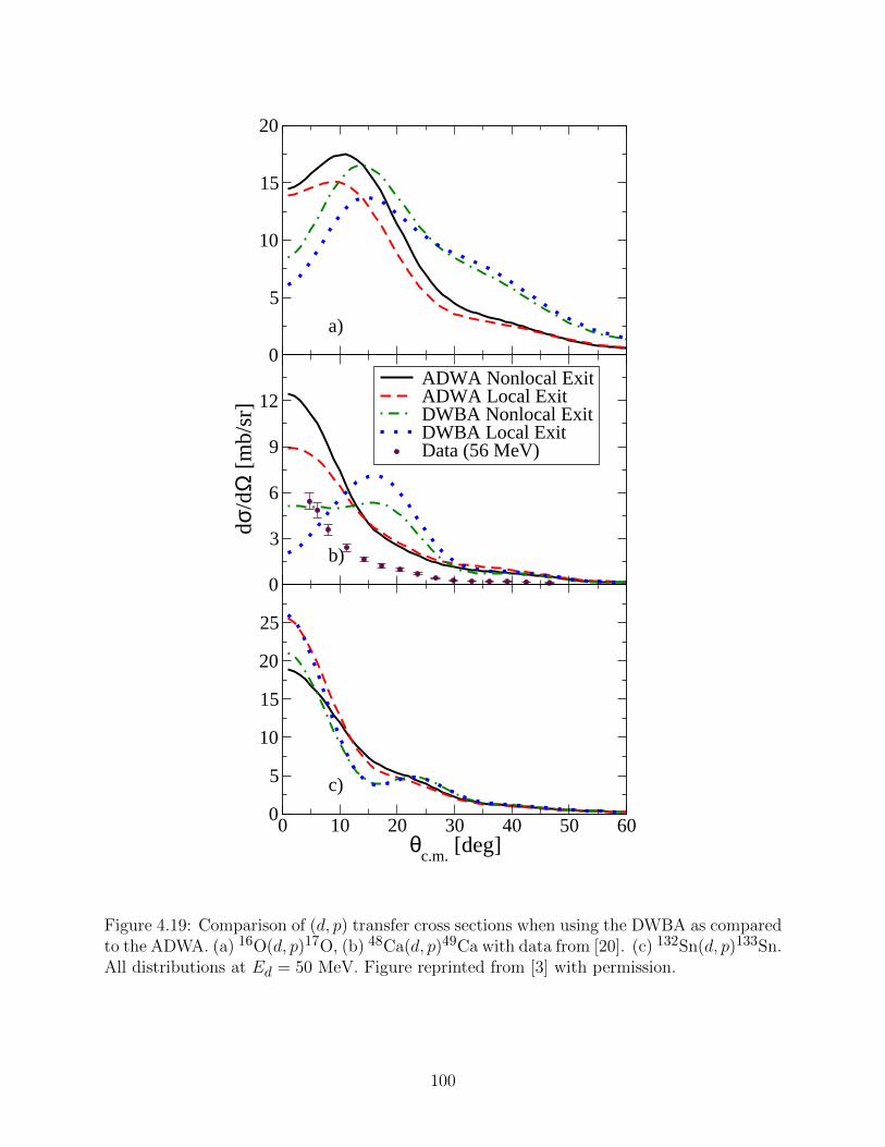
0

5

10

15

20

0

3

6

9

12

dσ/d

Ω [

mb/

sr]

ADWA Nonlocal ExitADWA Local ExitDWBA Nonlocal ExitDWBA Local ExitData (56 MeV)

0 10 20 30 40 50 60θ

c.m. [deg]

0

5

10

15

20

25

a)

b)

c)

Figure 4.19: Comparison of (d, p) transfer cross sections when using the DWBA as comparedto the ADWA. (a) 16O(d, p)17O, (b) 48Ca(d, p)49Ca with data from [20]. (c) 132Sn(d, p)133Sn.All distributions at Ed = 50 MeV. Figure reprinted from [3] with permission.

100

show the in Fig. 4.19b. It is clear that for this case, the DWBA is not able to describe the

angular distribution from experiment. This is one example that demonstrates the need to

explicitly include deuteron breakup into the calculation.

4.4.5 Energy Shift Method

Since many reaction problems are solved in coordinate based theories, local interactions have

been preferred due to the simplicity of solving the equations. For this reason, Timofeyuk

and Johnson, [21, 22], developed a method to effectively include nonlocality in the deuteron

scattering state within the formalism of the ADWA. Their method relies on local potentials

so that the nonlocal equation does not need to be solved. Assuming the Perey-Buck form

for the nonlocal potential, and through expansions, they find that by shifting the energy at

which the local potentials are evaluated by ∼ 40 MeV from the standard Ed/2 value, one

can capture the effects of nonlocality. Since we are now able to include nonlocality explicitly,

this method can be tested.

As we are only concerned with nonlocality in the deuteron channel, we fixed the potentials

in the proton channel so we can make a meaningful comparison. In the exit channel, the LPE

potentials found from fits to Perey-Buck proton elastic scattering distributions were used,

along with the local binding potential used to reproduce the experimental binding energy.

In the entrance channel, we used the nonlocal Perey-Buck potential, and the corresponding

LPE potentials. To use the method of [21, 22], we needed an energy dependent local optical

potential. For this we used the CH89 potential [23] evaluated at the standard Ed/2 value,

and with the additional energy shift that was quantified in [21].

The results of this study are shown in Fig. 4.20. We show angular distributions for (d, p)

reactions on (a) 16O at Ed = 10 MeV, (b) 40Ca at Ed = 10 MeV, and (c) 208Pb at Ed = 20

101

0

10

20

30

40

Nonlocal EntranceLocal EntranceCH89 + Energy ShiftCH89

0

2

4

6

8

0 20 40 60 80 100θ

c.m. [deg]

0

3

6

9

12

a)

b)

c)

Figure 4.20: Comparison of (d, p) angular distributions when using the energy shift methodof [21, 22]. (a) 16O(d, p)17O at Ed = 10 MeV (b) 40Ca(d, p)41Ca at Ed = 10 MeV (c)208Pb(d, p)209Pb at Ed = 20 MeV. The solid line is when full nonlocality was included inthe entrance channel, dashed line is when the LPE potential was used, dot-dashed line whenthe CH89 potential [23] was used with the additional energy shift quantified in [21], and thedotted line when the CH89 potential was used at the standard Ed/2 value. Figure reprintedfrom [3] with permission.

102

MeV. The solid line is the distribution form nonlocality explicitly included in the deuteron

channel, the dashed line are the results of the local calculations with the LPE potentials

for the deuteron scattering state, the dot-dashed line used the method of [21, 22], and the

dotted line is when the local potentials are evaluated at the standard Ed/2 value.

Our results show that the energy shift method always increases the cross section. How-

ever, the explicit inclusion of nonlocality in the deuteron scattering state can sometimes

decrease the cross section, as is seen in Fig. 4.20a. Often times, the energy shift moves the

transfer distribution towards larger angles, an effect also seen in the full nonlocal calcula-

tions. In some cases, the energy shift method over shoots the full nonlocal calculation, as

in Fig. 4.20b. In Fig. 4.20c, we see an example where the energy shift does a very good

job at reproducing the nonlocal effects. In general, we found that for most cases, the energy

shift captured the qualitative effects of nonlocality, but was unable to provide an accurate

account of the nonlocal effects.

4.4.6 Summary

In this work we studied the effects of nonlocality on (d, p) transfer reactions. An extension of

the ADWA theory was developed to include nonlocality in the deuteron scattering state using

the Perey-Buck nonlocal nucleon optical potential [1]. In the exit channel the Perey-Buck

potential was used to describe the proton scattering state, and its real part was adjusted

for the neutron bound state. For the scattering, a local phase equivalent (LPE) potential

was obtained by fitting the elastic scattering generated from the corresponding nonlocal

potential. Both the local and nonlocal bound states reproduced the same experimental

binding energies.

For the (d, p) reactions studied, we found that the inclusion of nonlocality in both the

103

entrance and exit channels increased the transfer cross section by ∼ 40%. In most cases,

nonlocality in the deuteron scattering state caused a moderate increase in the transfer cross

section. However, for heavy targets at high energies, this increase was large. Nonlocality

in the exit channel caused, almost exclusively, an increase in the transfer cross section,

except for heavy targets at high energies for which the cross sections were reduced. We also

compared our ADWA result with those from DWBA and found the effects of nonlocality in

the final state to be consistent in both formulations, even if quantitatively different. We also

compared our ADWA results with the energy shift method introduced by Timofeyuk and

Johnson [21, 22] and found that method to be qualitatively consistent with our results.

The conclusion of the present study confirm those of [12, 14]. There are important

differences in the transfer cross sections when including nonlocality explicitly as compared to

when using LPE potentials. This highlights the necessity of explicitly including nonlocality

to describe transfer reactions. Since the inclusion of nonlocality normally increases the

cross section, a re-analysis of transfer reaction data will likely reduce currenlty accepted

spectroscopic factors, such as those reported in [111].

104

Chapter 5

Conclusions and Outlook

5.1 Conclusions

In this thesis we studied the effect of nonlocality of the optical potential in transfer reactions.

For this purpose we developed a method for solving the integro-differential equations and

extended the adiabatic distorted wave approximation for transfer (d, p) reactions to include

nonlocal interactions of general form. We performed several systematic studies, including a

range of energies, targets, and interactions.

For the (p, d) reaction study using the Perey-Buck nonlocal potential of Sec. 4.2, we

considered a range of nuclei, and proton energies of Ep = 20 and 50 MeV [12]. We calculated

the transfer matrix element in the distorted wave Born approximation (DWBA), and used a

local optical potential to describe the deuteron scattering state. We found that the explicit

inclusion of nonlocality increased the transfer cross section at the first peak by 15 − 35%,

relative to when local potentials were use. We found that in all cases, the Perey correction

factor traditionally used does not provide a quantitative description. Our results suggest

that such a correction factor to account for nonlocality should not be used.

In Sec. 4.3 we compared the DOM potential and the Perey-Buck potential to study (p, d)

reactions on 40Ca at Ep = 20, 35, and 50 MeV [14]. We included nonlocality in the entrance

channel, then computed transfer cross sections in the DWBA, ignoring nonlocality in the

deuteron channel. We generated two local phase equivalent (LPE) potentials, one for the

105

DOM and one for the Perey-Buck potential. Both the DOM and the Perey-Buck potential

produced very large increases in the magnitude of the transfer cross section, ≈ 15− 50% for

the DOM potential, and ≈ 30 − 50% for the Perey-Buck potential. Like in the first study

of (p, d) reactions, when nonlocality was included only in the bound state, large increases in

the magnitude of the transfer cross section were seen. Typically, nonlocality in the proton

scattering state acts in the opposite direction, reducing the transfer cross section.

In the last study of Sec. 4.4 involving (d, p) reactions, nonlocality was included in the

deuteron channel within the adiabatic distorted wave approximation (ADWA), which unlike

the DWBA, includes deuteron breakup explicitly [3]. The formalism for the local ADWA

theory had to be extended to include nonlocal potentials, and was done in Sec. 2.6. We

found that the inclusion of nonlocality increased the transfer cross section by ∼ 40%. In most

cases, nonlocality in the deuteron scattering state caused a modest increase in the transfer

cross section. However, for heavy targets at high energy, the increase due to nonlocality in

the deuteron channel was very large. This is in contrast to when nonlocality is added to the

proton scattering state, which often times reduced the transfer cross section. The reason

for the difference is that nonlocality in the deuteron scattering state had both the effect of

reducing the magnitude of the scattering wave function within the nuclear interior, but also

shifting the wave function outwards towards the periphery.

All these three studies [12, 14, 3] demonstrate the important differences in the transfer

cross sections when including nonlocality explicitly, as compared to when using local phase

equivalent potentials. This emphasizes the necessity of including nonlocality to describe

transfer reactions if accurate structure information is to be extracted.

Most often, transfer reactions are performed to extract a spectroscopic factor. The analy-

sis is done using local potentials. As explicit inclusion of nonlocality increased the predicted

106

cross sections, one would expect lower spectroscopic factors to result from the analysis if

nonlocal potentials are used. This may well contribute to solving the discrepancy between

spectroscopic factors extracted from knockout and transfer [112], but that study has yet to

be performed.

5.2 Outlook

Going forward, nonlocality must be carefully taken into account in any advanced reaction

theory. It will become increasingly important to construct a modern nonlocal global optical

potential. Work along these lines has already been done by Tian, Pang, and Ma (TPM)

with the recent publication of their nonlocal potential, [2]. However, this potential is still

energy independent, and is based on the simple Perey-Buck form.

On physical grounds, the optical potential must be energy dependent due to channel

coupling effects. Preliminary indications from an unpublished study by Bacq, Lovell, Titus,

and Nunes [113] show that there is indeed an energy dependence in nonlocal potentials of the

Perey-Buck form. Work on specifying the precise energy dependence is ongoing. It would

be advantageous to construct an energy dependent nonlocal global optical potential through

χ2 minimization of a large quantity of elastic scattering angular distributions, and perhaps

polarization observables and other data as well.

The Perey-Buck form for the potential comprises a single nonlocality parameter, β. This

simple form has been useful for many decades since it allowed for simple implementation.

It is unlikely that a single nonlocality parameter is able to represent the complex nature

of nonlocality in the realistic many-body problem. The DOM potential, for example, has

a different β for each term of the potential. A more sophisticated form for the nonlocal

107

potential should be considered.

There are several methods available to construct a microscopically based optical poten-

tial. Some of these methods were discussed in Chapter 1, and should be pursued now that it

is known that nonlocality is very important and must be included explicitly. Since previous

microscopic calculations of nonlocal potentials have shown that their form does not resem-

ble the simple Gaussian nonlocality of the Perey-Buck potential, it is important to better

understand its analytic properties.

With an improved nonlocal global optical potential, existing transfer data can be re-

analyzed. The large discrepancies between spectroscopic factors extracted from the nonlocal

and local calculations in this study demonstrates that the structure information of most

nuclei are likely to be altered when the data is analyzed with nonlocal potentials.

While this thesis focused on (d, p) and (p, d) reactions, the role of nonlocality should be

investigated in other reactions as well. We are currently investigating the role of nonlocality

in (d, n) reactions [114]. Surprisingly, the effects of nonlocality in (d, n) reactions are even

more significant than in (d, p) reactions.

Along with transfer, there are many other reactions that are performed to extract sin-

gle particle structure of nuclei. Nuclear knockout reactions (A(a, bγ)X) are an alternative

method to extract a spectroscopic factor. Such a reaction also requires an optical potential

between the colliding nuclei. Understanding the effect of nonlocality in this case is also im-

portant. Inelastic scattering provides the transition strength between the ground state and a

bound excited state in a nucleus. Since these are obtained by comparing experimental data

to theoretical distributions resulting from a DWBA or coupled channel analysis, one may

again expect that inclusion of nonlocality in the description of the process will improve the

reliability of the extracted transition strength. Three-body models exist to calculate trans-

108

fer, such as the continuum discretized coupled channel method [95]. In this case, coupled

channel integro-differential equations would need to be solved, and new numerical methods

may be needed to accomplish this task. Finally, charge-exchange reactions, such as (p, n),

probe the spin and isospin properties of nuclei. Once again, information from experiments

are sometimes extracted from a DWBA analysis, and including nonlocality in the optical

potential will improve the reliability of theoretical predictions, consequently the reliability

of the extracted Gamow-Teller strengths.

One aspect that was not addressed in this thesis concerns error quantification. Lovell

and Nunes [115] are currently addressing error quantification in direct reaction theories when

using local potentials. An extension of that work will be necessary as the use of nonlocal

nonlocal potentials becomes more widespread. Much work has highlighted the importance

of nonlocality in the reaction dynamics. How then can we constrain nonlocality from data?

The Perey-Buck potential, for example, has a Gaussian form with a nonlocality range of

β = 0.85 fm. Elastic scattering is not sensitive to short-range properties, so constraining β

in this way may not be the best method. Reactions sensitive to short range correlations may

offer a better avenue.

The results of this thesis, along with the advent of microscopic theories to construct

nonlocal potentials, improved phenomenological nonlocal global optical potentials, and ever

increasing computer power, has the potential to elevate reaction theory to a new level.

While we have focused on (p, d) and (d, p) reactions, with our increased understanding of

nonlocality, it has become necessary to update the other formalisms and codes commonly

used in nuclear physics to properly include nonlocality in reaction theory.

109

APPENDICES

110

Appendix A

Solving the Nonlocal Equation

In order to assess the validity of the local approximation we need to solve Eq.(3.14) exactly.

Several methods exist for solving the scattering state, such as [78, 80]. Our approach follows

Perey and Buck [1] where Eq.(3.14) is solved by iteration. For simplicity, we will drop the

local part of the nonlocal potential, Uo(r), in our discussion, although it is included in our

calculations.

To solve the partial wave equation of Eq.(3.14) numerically, we need to find the kernel

function gL(R,R′). In order to do this, we first need to do a partial wave expansion of the

nonlocal potential,

UNLPB (R,R′) =∑L

2L+ 1

4π

gL(R,R′)RR′

PL(cos θ), (A.1)

where we defined θ as the angle between R and R′. Inserting the Perey-Buck form for the

nonlocal potential, multiplying both sides by PL(cos θ), integrating over all angles, using the

orthogonality of the Legendre polynomials, and solving for gL(R,R′), we find that

gL(R,R′) = 2πRR′U(

1

2(R +R′)

)∫ 1

−1

exp

(−∣∣∣R−R′β

∣∣∣2)π32β3

PL(cos θ)d(cos θ). (A.2)

111

For a moment, consider only the integral on the right:

∫ 1

−1

exp

(−∣∣∣R−R′β

∣∣∣2)π32β3

PL(cos θ)d(cos θ) =

exp

(−R

2+R′2β2

)π32β3

∫ 1

−1ei(−izcosθ)PL(cos θ)d(cos θ).

(A.3)

Using the integral representation for the spherical Bessel functions,

jL(x) =1

2iL

∫ 1

−1eixuPL(u)du, (A.4)

with u = cos θ, we find that

gL(R,R′) =2iLz

π12β

jL(−iz)exp

(−R

2 +R′2

β2

)U

(1

2(R +R′)

)= hL(R,R′)U

(1

2(R +R′)

). (A.5)

Calculating hL(R,R′) numerically is difficult for z 1 due to large cancellations between

the terms, so we need to approximate this function when doing numerical calculations for

large values of the argument. Making use of the asymptotic expression for the spherical Bessel

function, and neglecting terms proportional to exp

[−(R+R′β

)2], we find that hL(R,R′) for

z 1 can be approximated as

112

hL(R,R′) ≈ 1

π12βe−(R−R′β

)2for |z| 1. (A.6)

Scattering solutions are considered first, where the subscript n denotes the nth order

approximation of the correct solution. The iteration scheme starts with an initialization,

~2

2µ

[d2

dr2− L(L+ 1)

R2

]χn=0(R) + [E − Uinit(R)]χn=0(R) = 0, (A.7)

where Uinit(R) is some suitable local potential used to get the iteration process started.

Knowing χo(R) one then proceeds with solving:

~2

2µ

[d2

dr2− L(L+ 1)

R2

]χn(R) + [E − Uinit(R)]χn(R)

=

∫gL(R,R′)χn−1(R′)dR′ − Uinit(R)χn−1(R), (A.8)

with as many iterations necessary for convergence. The number of iterations depends mostly

on the partial wave being solved for (lower partial waves require more iterations) and the

quality of Uinit(R). It was rare for any partial wave to require more than 20 iterations to

converge, even with a very poor choice for Uinit(R). If the LPE potential is used as Uinit(R),

then any partial wave converges with less than 10 iterations.

For the bound state problem, the method is somewhat different. A variety of methods

exist in the literature, some developed specifically to handle non-analytic forms (e.g. [81]).

Our approach may not be the most efficient, but it is straightforward, general, and easy to

implement. To solve the bound state problem with a nonlocal potential we begin by solving

113

Eq.(A.7). Since we are using the wave function from the previous iteration to calculate the

nonlocal integral, we need to keep track of the different normalizations of the inward and

outward wave functions that results from the choice for the initial conditions for each wave

function. Thus, the equations we iterate are:

~2

2µ

[d2

dr2− `(`+ 1)

r2

]φInn (r) + [E − Uinit(r)]φInn (r)

=

∫ RMax

0g`(r, r

′)φInn−1(r′)dr′ − Uinit(r)φInn−1(r), (A.9)

and

~2

2µ

[d2

dr2− `(`+ 1)

r2

]φOutn (r) + [E − Uinit(r)]φOutn (r)

=

∫ RMax

0g`(r, r

′)φOutn−1(r′)dr′ − Uinit(r)φOutn−1(r), (A.10)

where RMax is some maximum radius chosen greater than the range of the nuclear interac-

tion. Note that φIn(r) is the wave function for integrating from the edge of the box inward

and has a normalization set by the Whittaker function as the initial condition, while φOut(r)

is the wave function for integrating from the origin outward and has the normalization set

using the standard rL+1 initial condition near the origin.

Even though φOut and φIn differ by only a constant, these two equations (Eq.(A.9) and

Eq.(A.10)) are necessary because the value of the normalization constant is only known after

convergence. For a given iteration, φOut and φIn converge when their logarithmic derivatives

agree at the matching point. To keep the proper normalization throughout the entire range

114

[0, RMax], we need to retain two versions of the converged wave function for each iteration:

φInn (r) =

COutn φOut

n (r) for 0 ≤ r < RMatch

φInn (r) for RMatch ≤ r ≤ RMax

(A.11)

φOutn (r) =

φOutn (r) for 0 ≤ r < RMatch

CInn φ

Inn (r) for RMatch ≤ r ≤ RMax

(A.12)

where

CIn(Out) =φOut(In)(RMatch)

φIn(Out)(RMatch)(A.13)

The full iteration scheme is converged when the binding energy obtained from the previous

iteration agrees with the binding energy from the current iteration within a desired level of

accuracy. Again, although this may not be the most efficient method, it is general (whatever

the form of nonlocality) and is very stable, providing a good option for future studies beyond

the Perey-Buck potentials.

115

Appendix B

Deriving the Perey Correction Factor

Here we provide details on the derivation of the PCF, Eq. (3.18). We also include the

derivation of the transformation formulas, as well as the correct radial version of the trans-

formation formulas which could be used to transform the nonlocal radius and diffuseness to

their local counterpart.

We start from Eq. (3.15). Let us define a function F (R) that connects the local wave

function ΨLoc(R), resulting from the potential ULE(R), with the wave function resulting

from a nonlocal potential, ΨNL(R):

ΨNL(R) ≡ F (R)ΨLoc(R). (B.1)

Since the local and nonlocal equations describe the same elastic scattering, the wave

functions should be identical outside the nuclear interior. Thus, F (R) → 1 as R → ∞.

By inserting Eq.(B.1) into the nonlocal equation Eq.(3.15) we can reduce the result to the

following local equivalent equation

−~2

2µ∇2ΨLoc(R) + ULE(R)ΨLoc(R) = EΨLoc(R), (B.2)

where the local equivalent potential is given by:

116

ULE(R) =−~2µ ∇F (R) · ∇ΨLoc(R)− ~2

2µ(∇2F (R))ΨLoc(R)

F (R)ΨLoc(R)

+

∫UNL(R,R′)F (R′)ΨLoc(R′)dR′

F (R)ΨLoc(R)+ Uo(R).

(B.3)

We next consider the numerator of the second term of Eq.(B.3) and introduce the explicit

nonlocal potential form of Eq.(3.9). Using the definition s = R −R′, expanding in powers

of s up to first order, the integral becomes

∫UNLWS

(∣∣∣∣R− 1

2s

∣∣∣∣)H(s)F (R− s)ΨLoc(R− s)ds

≈ UNLWS(R)F (R)

∫H(s)ΨLoc(R− s)ds− 1

2F (R)∇UNLWS(R) ·

∫sH(s)ΨLoc(R− s)ds

− UNLWS(R)∇F (R) ·∫

SH(s)ΨLoc(R− s)ds, (B.4)

where

H(s) =

exp

(− s2

β2

)π3/2β3

. (B.5)

Therefore, the local equivalent potential becomes:

117

ULE(R) ≈ 1

F (R)ΨLoc(R)

[−~2

µ(∇F · ∇ΨLoc)

+ UNLWS(R)F (R)

∫H(s)ΨLoc(R− s)ds

− 1

2F (R)∇UNLWS ·

∫sH(s)ΨLoc(R− s)ds

− UNLWS(R)∇F ·∫

sH(s)ΨLoc(R− s)ds

]− ~2

2µ

∇2F (R)

F (R)+ Uo(R). (B.6)

Consider the four terms in the brackets. All of these terms are divided by ΨLoc, which

has nodes. The first, third, and fourth terms depend on dot products and gradients of ΨLoc.

These terms are unlikely to individually equal zero when ΨLoc in the denominator equals

zero. Thus, we require that these terms sum to zero so that ULE(R) remains finite. As

pointed out in [74], this is not an approximation, but merely a condition for the method to

work. Applying this condition gives us two equations:

ULE(R) = UNLWS(R)

[∫H(s)ΨLoc(R− s)ds

ΨLoc(R)

]+ Uo(R)− ~2

2µ

∇2F (R)

F (R)(B.7)

0 =~2

µ(∇F · ∇ΨLoc) +

[1

2F (R)∇UNLWS + UNLWS(R)∇F

]·∫

sH(s)ΨLoc(R− s)ds.

(B.8)

Instead of using the local WKB approximations as Austern did [74], we use the operator

118

form of the Taylor expansion to factorize the wave function:

ΨLoc(R− s) = e−is·kΨLoc(R), (B.9)

with k = −i∇. This simplifies the integrals in Eq.(B.7) and Eq.(B.8). Consider first the

integral in Eq.(B.7)

∫H(s)ΨLoc(R− s)ds =

[∫e−is·kH(s)ds

]ΨLoc(R)

= exp

[−k2β2

4

]ΨLoc(R). (B.10)

Therefore, assuming the potentials are scalar functions of R, and replacing Eq.(B.10) into

Eq.(B.7) we obtain;

ULE(R) = UNLWS(R) exp

[−µβ

2

2~2(E − ULE(R)

)]+ Uo(R)− ~2

2µ

∇2F (R)

F (R), (B.11)

where we used k2 = −∇2 in the exponent to first order, and the Schrodinger’s equation.

Making the replacement ULE(R) = ULocWS(R) + Uo(R), gives us the radial transformation

formula

UNLWS(R) =

(ULocWS(R) +

~2

2µ

∇2F (R)

F (R)

)exp

[µβ2

2~2(E − ULocWS(R)− Uo(R)

)].

The ∇2F term is significant around the surface, but near the origin this term is negligible.

119

Therefore, if we neglect this term, then we must remove the radial arguments, and consider

this formula only near the origin. Therefore, for R ≈ 0

UNLWS(0) ≈ ULocWS(0) exp

[µβ2

2~2(E − ULocWS(0)− Uo(0)

)]. (B.12)

The UWS(R) functions are of a Woods-Saxon form, and have real and imaginary parts

UWS(R) = UR(R) + iUI(R) (B.13)

=−Vv

1 + exp

(R−rA1/3

a

) + 4i

−Wd exp

(R−rA1/3

a

)(

1 + exp

(R−rA1/3

a

))2.

Inserting this into Eq.(B.12) we obtain;

UNLR (R) + iUNLI (R) = (ULocR (R) + iULocI (R))

× exp

[µβ2

2~2(E − Uo(R)− ULocR (r)− iULocI (R)

)].

(B.14)

Near the origin, ULocI ≈ 0 so this term can be neglected in the exponent, and UR ≈ −Vv.

While the spin-orbit term diverges at the origin, it rapidly goes to zero away from the origin,

so we assume the spin-orbit contribution is negligible. Thus, Uo = Vc, where Vc is the

Coulomb potential at the origin for a uniform sphere of charge. Taking the real part of the

above equation and making these substitutions gives

120

V NLv = V Locv exp

[µβ2

2~2(E − Vc + V Locv

)]. (B.15)

For the imaginary part, we have:

UNLI (R) = ULocI (R) exp

[µβ2

2~2(E − Vc + V Locv

)]. (B.16)

While UI(R) ≈ 0 near the origin, the local and nonlocal terms have the same form factor, so

the form factors exactly cancel as long as the radius and diffuseness are identical. Therefore,

the imaginary part of Eq.(B.14) gives

WNLd = WLoc

d exp

[µβ2

2~2(E − Vc + V Locv

)], (B.17)

It is important to note that these equations are only valid for transforming the depths of the

potentials, thus Eq.(B.12) should not be used while retaining the radial dependence. Indeed,

Eq.(A13) is not valid for all R.

Now consider the integral in Eq.(B.8). Using Eq.(B.9) to expand the wave function, and

evaluating the dot product we get

0 =~2

µ(∇F · ∇ΨLoc) +

[1

2F (R)∇UNLWS + UNLWS(R)∇F

]×[∫

s cos(θ)H(s)e−is·kds]

ΨLoc(R). (B.18)

Doing the integral, we find that this becomes

121

0 =~2

µ∇F −

[1

2F (R)(∇UNLWS) + UNLWS(R)(∇F )

]×β

2

2exp

[−µβ

2

2~2(E − ULE(R)

)]. (B.19)

If we assume that the local momentum approximation is valid, this equation can be solved

exactly and has the solution

F (R) =

[1− µβ2

2~2UNLWS(R) exp

(−µβ

2

2~2(E − ULE(R)

))]−12. (B.20)

If the local momentum approximation is not valid, then insertion of Eq.(B.20) into the rhs

of Eq.(B.19) will deviate from zero by a term related to the derivative of ULE(R). This

additional term will be significant at the surface, and thus one can expect discrepancies in

applying Eq.(B.20) in this region.

Comparing Eq.(B.20) with Eq.(B.11) we see that

F (R) =

[1− µβ2

2~2

(ULE(R)− Uo(R) +

~2

2µ

∇2F (R)

F (R)

)]−12. (B.21)

Neglecting the term containing ∇2F gives us Eq.(3.18), which is the correction factor of

Austern [74]. The contribution of ∇2F/F is only important at the surface, and again it is

precisely for these radii that discrepancies can be expected in applying Eq.(3.18).

122

Appendix C

Nonlocal Adiabatic Potential

Here we will derive the nonlocal adiabatic potential. We begin with a three-body Schrodinger

Equation:

[TR + Tr + Vnp(r) + UnA + UpA − E

]Ψ(r,R) = 0. (C.1)

We expand the wave function using Weinberg states,

Ψ(r,R) =∞∑i=0

Φi(r)Xi(R), (C.2)

and keep only the first Weinberg State,

Ψ(r,R) ≈ Φo(r)Xo(R) = Φ(r)X(R). (C.3)

Noting that

(Tr + Vnp)Φ(r) = −εdΦ(r), (C.4)

with Ed = E + εd, the Schrodinger equation becomes

123

[TR − Ed

]Φ(r)X(R) = −

[UnA + UpA

]Φ(r)X(R). (C.5)

Now we evaluate the nucleon nonlocal operator, UNAΦ(r)X(R). For a moment, consider

just the neutron potential (with Rp,n = R± r2 where the “+” sign is for the proton and the

“-” sign is for the neutron)

UnAΨ(r,R) = UnAΨ(Rn,Rp)

=

∫U(Rn,R

′n)Ψ(R′n,Rp)δ(R

′p −Rp)dR

′pdR

′n (C.6)

= J∫U

(R− r

2,R′ − r′

2

)Ψ(r′,R′)δ(R′p −Rp)dr

′dR′

= J∫U

(R− r

2,R′ − r′

2

)Ψ(r′,R′)δ

(R′ +

r′

2− (R +

r

2)

)dr′dR′

= 8J∫U

(R− r

2,R′ − r′

2

)Ψ(r′,R′)δ

(r′ − (r− 2(R′ −R))

)dr′dR′

The Jacobian for the coordinate transformation is

J =

∣∣∣∣∣∣∣∂R′n∂R′

∂R′n∂r′

∂R′p∂R′

∂R′p∂r′

∣∣∣∣∣∣∣ =

∣∣∣∣∣∣∣1 −1

2

1 12

∣∣∣∣∣∣∣ = 1, (C.7)

which gives us

UnAΨ(r,R) = 8

∫UnA

(R− r

2,R′ − r− 2(R′ −R)

2

)Ψ(r− 2(R′ −R),R′

)dR′

= 8

∫UnA

(R− r

2, 2R′ −R− r

2

)Ψ(r− 2(R′ −R),R′)dR′. (C.8)

124

For the nucleon nonlocal operator, we have

UNAΦ(r)X(R) = 8

∫UNA

(R± r

2, 2R′ −R± r

2

)Φ(r± 2(R′ −R))X(R′)dR′.

(C.9)

Consider the argument of UNA. Adding and subtracting by R in the second argument we

get

UNA

(R± r

2, 2R′ −R± r

2

)= UNA

(Rp,n, 2R′ −R−R + R± r

2

)= UNA

(Rp,n, 2(R′ −R) + Rp,n

)= UNA

(Rp,n,Rp,n + 2s

), (C.10)

where we made the definition, s = R′ − R. Since dR′ → ds, we see that UNAΦ(r)X(R)

becomes

UNAΦ(r)X(R) = 8

∫UNA

(Rp,n,Rp,n + 2s

)Φ(r± 2s)X(R + s)ds. (C.11)

The general expansion of the full wave function for a given partial wave with total angular

momentum JT and projection MT , is given by

125

Ψ(r,R) ≈ Φ(r)X(R) =∑L′J ′p

Φ(r)⊗ YL′(R)

J ′p⊗ ΞIt(ξt)

JTMT

χJTMTL′J ′p

(R)

=∑`′L′J ′p

ΞId

(ξnp)⊗ Y`′(r)Jd⊗ YL′(R)

J ′p⊗ ΞIt(ξt)

JTMT

× φ`′(r)χJTMTL′J ′p

(R)

R, (C.12)

where

ΞId(ξnp) =

ΞIp(ξp)⊗ ΞIn(ξn)

Id. (C.13)

In these equations, ΞIp(ξp), ΞIn(ξn) and ΞIt(ξt) are the spin functions for the proton, neu-

tron, and target, respectively. Ip = In = 1/2 are the spin of the proton and neutron

respectively, and It is the spin of the target. YL(R) is the spherical harmonic for the orbital

motion between the projectile and target, while Y`(r) is for the internal orbital angular mo-

mentum of the deuteron. We are using the phase convention where there is a built in factor

of iL so that YL(R) = iLYL(R) where YL(R) is defined on [93], p.133, Eq.(1). The spin of

the deuteron is given by Id = 1 and the total angular momentum of the deuteron is Jd = 1.

The total angular momentum of the deuteron is coupled to the orbital angular momentum

between the deuteron and target to give a total angular momentum of the projectile, Jp.

The total angular momentum of the projectile is coupled to the spin of the target to give

the total angular momentum of the system, JT with projection MT .

The Schrodinger equation is now

126

[TR − Ed

]Φ(r)X(R) = −UNAΦ(r)X(R)

= −8

∫UNA

(Rp,n,Rp,n + 2s

)Φ(r± 2s)X(R + s)ds

= −∑`′L′J ′p

8

∫UNA

(Rp,n,Rp,n + 2s

)

×

ΞId

(ξnp)⊗ Y`′(r ± 2s)Jd⊗ YL′(R + s)

J ′p⊗ ΞIt(ξt)

JTMT

× φ`′(|r± 2s|)χJTMTL′J ′p

(|R + s|)

|R + s|ds. (C.14)

We would like to do a partial wave decomposition to get an equation for each LJ combination

of the scattering wave function. To do this, multiply both sides of Eq.(C.14) by

∑`

ΞId

(ξnp)⊗ Y`(r)Jd⊗ YL(R)

Jp

⊗ ΞIt(ξt)

∗JTMT

φ`(r)Vnp(r), (C.15)

and integrate over dr, dΩR, dξnp, and dξt, where dξnp = dξndξp. Consider first just the lhs

of Eq.(C.14) after multiplication of Eq.(C.15),

127

∫ ∑`

ΞId

(ξnp)⊗ Y`(r)Jd⊗ YL(R)

Jp

⊗ ΞIt(ξt)

∗JTMT

φ`(r)Vnp(r)

×[TR − Ed

] ∑`′L′J ′p

ΞId

(ξnp)⊗ Y`′(r)Jd⊗ YL′(R)

J ′p⊗ ΞIt(ξt)

JTMT

× φ`′(r)χJTMTL′J ′p

(R)

RdrdΩR

= −∑`

∑`′L′J ′p

1

R

[~2

2µ

(∂2

∂R2− L′(L′ + 1)

R2

)+ Ed

]χJTMTL′J ′p

(R)

∫φ`(r)Vnp(r)φ`′(r)r

2dr

×∫

ΞId(ξnp)⊗ Y`(r)

Jd⊗ YL(R)

Jp

⊗ ΞIt(ξt)

∗JTMT

(C.16)

×

ΞId

(ξnp)⊗ Y`′(r)Jd⊗ YL′(R)

J ′p⊗ ΞIt(ξt)

JTMT

dΩrdΩRdξnpdξt.

Next we consider the integral in the last two lines of Eq.(C.16)

∫ ΞId

(ξnp)⊗ Y`(r)Jd⊗ YL(R)

Jp

⊗ ΞIt(ξt)

∗JTMT

×

ΞId

(ξnp)⊗ Y`′(r)Jd⊗ YL′(R)

J ′p⊗ ΞIt(ξt)

JTMT

dΩrdΩRdξnpdξt

=∑

MpM ′p

∫ ΞId

(ξnp)⊗ Y`(r)Jd⊗ YL(R)

∗JpMp

×

ΞId(ξnp)⊗ Y`′(r)

Jd⊗ YL′(R)

J ′pM ′p

dΩrdΩRdξnp

×∑µ′tµt

CJTMTJpMpItµt

CJTMTJ ′pM ′pItµ′t

∫Ξ∗Itµt(ξt)ΞItµ′t

(ξt)dξt. (C.17)

Evaluating the integral,∫

Ξ∗Itµt(ξt)ΞItµ

′t(ξt)dξt = δµtµ

′t, summing over µ′t, and evaluating

128

the complex conjugate using [93], p.62, Eq.(6), gives

=∑

MpM ′p

∑µt

CJTMTJpMpItµt

CJTMTJ ′pM ′pItµt

∫ ΞId

(ξnp)⊗ Y`(r)Jd⊗ YL(R)

∗JpMp

×

ΞId(ξnp)⊗ Y`′(r)

Jd⊗ YL′(R)

J ′pM ′p

dΩrdΩRdξnp

=∑

MpM ′p

∑µt

CJTMTJpMpItµt

CJTMTJ ′pM ′pItµt

×∫

(−)Jp−Mp

ΞId(ξnp)⊗ Y`(r)

Jd⊗ YL(R)

Jp,−Mp

×

ΞId(ξnp)⊗ Y`′(r)

Jd⊗ YL′(R)

J ′pM ′p

dΩrdΩRdξnp. (C.18)

Coupling the tensors up to zero angular momentum provides further simplifications:

ΞId

(ξnp)⊗ Y`(r)Jd⊗ YL(R)

Jp,−Mp

ΞId

(ξnp)⊗ Y`′(r)Jd⊗ YL′(R)

J ′pM ′p

=∑SMS

CSMSJp,−MpJ ′pM ′p

ΞId

(ξnp)⊗ Y`(r)Jd⊗ YL(R)

Jp

⊗

ΞId(ξnp)⊗ Y`′(r)

Jd⊗ YL′(R)

J ′p

SMS

→ C00Jp,−MpJ ′pM ′p

ΞId

(ξnp)⊗ Y`(r)Jd⊗ YL(R)

Jp

⊗

ΞId(ξnp)⊗ Y`′(r)

Jd⊗ YL′(R)

J ′p

00

. (C.19)

Next we consider just an ` = 0 deuteron. Therefore, Jd = Id, and we get,

129

1

4πC00Jp,−MpJ ′pM ′p

ΞId

(ξnp)⊗ YL(R)Jp⊗

ΞId(ξnp)⊗ YL′(R)

J ′p

00

. (C.20)

Putting this into Eq.(C.18), we get

−∑L′J ′p

1

R

[~2

2µ

(∂2

∂R2− L′(L′ + 1)

R2

)+ Ed

]χJTMTL′J ′p

(R)

∫φ`(r)Vnp(r)φ`′(r)r

2dr

×∑

MpM ′p

∑µt

CJTMTJpMpItµt

CJTMTJ ′pM ′pItµt

1

4πC00Jp,−MpJ ′pM ′p

(−)Jp−Mp (C.21)

×∫

ΞId(ξnp)⊗ YL(R)

Jp⊗

ΞId(ξnp)⊗ YL′(R)

J ′p

00

dΩrdΩRdξnp.

The integral over dΩr gives 4π and cancels the 1/4π already there, which leaves us with

−∑L′J ′p

1

R

[~2

2µ

(∂2

∂R2− L′(L′ + 1)

R2

)+ Ed

]χJTMTL′J ′p

(R)

∫φ`(r)Vnp(r)φ`′(r)r

2dr

×∑

MpM ′p

∑µt

CJTMTJpMpItµt

CJTMTJ ′pM ′pItµt

C00Jp,−MpJ ′pM ′p

(−)Jp−Mp

×∫

ΞId(ξnp)⊗ YL(R)

Jp⊗

ΞId(ξnp)⊗ YL′(R)

J ′p

00

dΩRdξnp (C.22)

We can use, [93], p.248, Eq.(1)

C00Jp,−MpJpMp = (−)Jp+Mp

δJpJ ′pδMp,M ′pJp

. (C.23)

130

Inserting Eq.(C.23) into Eq.(C.22), and summing over J ′p and M ′p (using [93], p.236, Eq.(8))

we get,

−∑L′

1

R

[~2

2µ

(∂2

∂R2− L′(L′ + 1)

R2

)+ Ed

]χJTMTL′Jp

(R)

∫φ`(r)Vnp(r)φ`′(r)r

2dr

×∑Mp

∑µt

CJTMTJpMpItµt

CJTMTJpMpItµt

(−)2Jp1

Jp(C.24)

×∫

ΞId(ξnp)⊗ YL(R)

Jp⊗

ΞId(ξnp)⊗ YL′(R)

Jp

00dΩRdξnp

= −∑L′

1

R

[~2

2µ

(∂2

∂R2− L′(L′ + 1)

R2

)+ Ed

]χJTMTL′Jp

(R)

∫φ`(r)Vnp(r)φ`′(r)r

2dr

× (−)2Jp1

Jp

∫ ΞId

(ξnp)⊗ YL(R)Jp⊗

ΞId(ξnp)⊗ YL′(R)

Jp

00dΩRdξnp.

Coupling the spin functions together and the spherical harmonics together, each up to zero

angular momentum, using [93], p.70, Eq. (11), and p.358 Eq.(4),

ΞId

(ξnp)⊗ YL(R)Jp⊗

ΞId(ξnp)⊗ YL′(R)

Jp

00

= J2p

Id L Jp

Id L′ Jp

0 0 0

ΞId(ξnp)⊗ ΞId

(ξnp)0⊗YL(R)⊗ YL′(R)

0

00

=JpδLL′

IdL

ΞId

(ξnp)⊗ ΞId(ξnp)

0⊗YL(R)⊗ YL′(R)

0

00. (C.25)

Replacing Eq.(C.25) into Eq.(C.24), and summing over L′, we obtain:

131

− 1

R

[~2

2µ

(∂2

∂R2− L′(L′ + 1)

R2

)+ Ed

]χJTMTL′Jp

(R)

∫φ`(r)Vnp(r)φ`′(r)r

2dr

× (−)2Jp(

1

Id

∫ ΞId

(ξnp)⊗ ΞId(ξnp)

00dξnp

)(1

L

∫ YL(R)⊗ YL(R)

00dΩR

)(C.26)

The integral over the two Weinberg states multiplied by Vnp gives −1 by the normalization

condition of Eq.(2.37). Also, since Id = 1, Jp is an integer, so (−)2Jp = 1. Thus, we have

1

R

[~2

2µ

(∂2

∂R2− L′(L′ + 1)

R2

)+ Ed

]χJTMTL′Jp

(R) (C.27)

×(

1

Id

∫ ΞId

(ξnp)⊗ ΞId(ξnp)

00dξnp

)(1

L

∫ YL(R)⊗ YL(R)

00dΩR

).

The integral over the spin functions can be worked out with Eq.(11), p.70, and Eq.(4), p.358

of [93]:

∫ ΞId

(ξnp)⊗ ΞId(ξnp)

00dξnp

=

∫ Ξ1/2(ξn)⊗ Ξ1/2(ξp)

1⊗

Ξ1/2(ξn)⊗ Ξ1/2(ξp)1

00dξndξp

=

∫12

12

12 1

12

12 1

0 0 0

Ξ1/2(ξn)⊗ Ξ1/2(ξn)0⊗

Ξ1/2(ξp)⊗ Ξ1/2(ξp)0

00dξndξp

=

∫12

12

21

∫ Ξ1/2(ξn)⊗ Ξ1/2(ξn)

00dξn

∫ Ξ1/2(ξp)⊗ Ξ1/2(ξp)

00dξp. (C.28)

132

Doing the integral over the neutron spin functions by using Eq.(13), p.132, and Eq.(1), p.248,

of [93] we arrrive at:

∫ Ξ1/2(ξn)⊗ Ξ1/2(ξn)

00dξn

=∑µn

∫C001/2,−µn,1/2,µnΞ1/2,−µn(ξn)Ξ1/2,µn(ξn)dξn

=∑µn

C001/2,−µn,1/2,µn(−)−1/2−µn

∫Ξ∗1/2µn(ξn)Ξ1/2,µn(ξn)dξn

=∑µn

(−)1/2+µn(12

) (−)−1/2−µn∫

Ξ∗1/2,µn(ξn)Ξ1/2,µn(ξn)dξn

=√

2, (C.29)

A similar procedure is followed for the integral over the proton spin functions. Thus, with

Id = 1

1

Id

∫ ΞId

(ξnp)⊗ ΞId(ξnp)

00dξnp = 1. (C.30)

The final integral in Eq.(C.27) can be worked out using Eq.(6), p.62, and Eq.(1), p.248, of

[93]

133

1

L

∫ YL(R)⊗ YL(R)

00dΩR =

1

L

∑M

C00L,−MLM

∫YL,−M (R)YLM (R)dΩR

=1

L

∑M

C00L,−MLM (−)−L+M

∫Y ∗LM (R)YLM (R)dΩR

=1

L

∑M

(−)L+M

L(−)−L+M = 1. (C.31)

Therefore, introducing Eq.(C.31) into Eq.(C.27) and joining the rhs of Eq.(C.16) we obtain:

1

R

[~2

2µ

(∂2

∂R2− L(L+ 1)

R2

)+ Ed

]χJTMTLJp

(R)

= −∑`′L′J ′p

∑`

8

∫ ΞId

(ξnp)⊗ Y`(r)jp⊗ YL(R)

Jp

⊗ ΞIt(ξt)

∗JTMT

× UNA(Rp,n,Rp,n + 2s

)×

ΞId

(ξnp)⊗ Y`′(r ± 2s)jp⊗ YL′(R + s)

J ′p⊗ ΞIt(ξt)

JTMT

× φ`(r)Vnp(r)φ`′(|r± 2s|)χJTMTL′J ′p

(|R + s|)

|R + s|dsdrdΩRdξtdξnp (C.32)

We now concentrate on the tensor couplings in the rhs of Eq.(C.32). First, we introduce

` = 0 for the deuteron, and integrate over dξt:

134

ΞId

(ξnp)⊗ Y0(r)jp⊗ YL(R)

Jp

⊗ ΞIt(ξt)

∗JTMT

×

ΞId

(ξnp)⊗ Y0(r ± 2s)jp⊗ YL′(R + s)

J ′p⊗ ΞIt(ξt)

JTMT

=1

4π

ΞId

(ξnp)⊗ YL(R)Jp⊗ ΞIt(ξt)

∗JTMT

×

ΞId(ξnp)⊗ YL′(R + s)

J ′p⊗ ΞIt(ξt)

JTMT

=1

4π

∑MpM ′p

∑µtµ′t

CJTMTJpMpItµt

CJTMTJ ′pM ′pItµ′t

ΞId

(ξnp)⊗ YL(R)∗JpMp

×

ΞId(ξnp)⊗ YL′(R + s)

J ′pM ′p

∫Ξ∗Itµt(ξt)ΞItµ′t

(ξt)dξt

=1

4π

∑MpM ′p

∑µt

CJTMTJpMpItµt

CJTMTJ ′pM ′pItµt

ΞId

(ξnp)⊗ YL(R)∗JpMp

×

ΞId(ξnp)⊗ YL′(R + s)

J ′pM ′p

.

(C.33)

Inserting Eq.(C.33) into Eq.(C.32) we arrive at:

1

R

[~2

2µ

(∂2

∂R2− L(L+ 1)

R2

)+ Ed

]χJTMTLJp

(R)

= − 1

4π

∑L′J ′p

8

∫φ0(r)Vnp(r)UNA

(Rp,n,Rp,n + 2s

)×∑

MpM ′p

∑µt

CJTMTJpMpItµt

CJTMTJ ′pM ′pItµt

ΞId

(ξnp)⊗ YL(R)∗JpMp

(C.34)

×

ΞId(ξnp)⊗ YL′(R + s)

J ′pM ′p

φ0(|r± 2s|)χJTMTL′J ′p

(|R + s|)

|R + s|dsdrdΩRdξnp.

135

Next we couple the two tensors together up to zero angular momentum using, Eq.(6), p.62,

and Eq.(1), p.248, of [93]:

ΞId

(ξnp)⊗ YL(R)∗JpMp

ΞId

(ξnp)⊗ YL′(R + s)J ′pM ′p

= (−)Jp−Mp

ΞId(ξnp)⊗ YL(R)

Jp,−Mp

ΞId

(ξnp)⊗ YL′(R + s)J ′pM ′p

= (−)Jp−Mp∑SMS

CSMSJp,−MpJ ′pMp

×

ΞId(ξnp)⊗ YL(R)

Jp⊗

ΞId(ξnp)⊗ YL′(R + s)

J ′p

00

→ (−)Jp−MpC00Jp,−MpJ ′pMp

×

ΞId(ξnp)⊗ YL(R)

Jp⊗

ΞId(ξnp)⊗ YL′(R + s)

J ′p

00

= (−)Jp−Mp(−)Jp+MpδJpJ ′p

δMpM ′pJp

×

ΞId(ξnp)⊗ YL(R)

Jp⊗

ΞId(ξnp)⊗ YL′(R + s)

J ′p

00

(C.35)

= (−)2JpδJpJ ′p

δMpM ′pJp

ΞId

(ξnp)⊗ YL(R)Jp⊗

ΞId(ξnp)⊗ YL′(R + s)

J ′p

00

.

We replace Eq.(C.35) in Eq.(C.34) and sum over J ′p and M ′p to obtain:

136

1

R

[~2

2µ

(∂2

∂R2− L(L+ 1)

R2

)+ Ed

]χJTMTLJp

(R)

= − 1

4π

∑L′

8

∫φ0(r)Vnp(r)UNA

(Rp,n,Rp,n + 2s

)×∑Mp

∑µt

CJTMTJpMpItµt

CJTMTJpMpItµt

(−)2Jp1

Jp

×

ΞId(ξnp)⊗ YL(R)

Jp⊗

ΞId(ξnp)⊗ YL′(R + s)

Jp

00

× φ0(|r± 2s|)χJTMTL′Jp

(|R + s|)

|R + s|dsdrdΩRdξnp. (C.36)

Next we sum over Mp and µt using, Eq.(8), p.236, of [93],

1

R

[~2

2µ

(∂2

∂R2− L(L+ 1)

R2

)+ Ed

]χJTMTLJp

(R)

= − 1

4π

∑L′

8

∫φ0(r)Vnp(r)UNA

(Rp,n,Rp,n + 2s

)×(−)2Jp

1

Jp

ΞId

(ξnp)⊗ YL(R)Jp⊗

ΞId(ξnp)⊗ YL′(R + s)

Jp

00

× φ0(|r± 2s|)χJTMTL′Jp

(|R + s|)

|R + s|dsdrdΩRdξnp. (C.37)

We now use Eq.(11), p.70, and Eq.(4), p.358, of [93] to couple the spin functions and the

spherical harmonics to zero angular momentum,

137

ΞId

(ξnp)⊗ YL(R)Jp⊗

ΞId(ξnp)⊗ YL′(R + s)

Jp

00

= J2p

Id L Jp

Id L′ Jp

0 0 0

ΞId(ξnp)⊗ ΞId

(ξnp)0⊗YL(R)⊗ YL′(R + s)

0

00

= δLL′Jp

IdL

ΞId

(ξnp)⊗ ΞId(ξnp)

0⊗YL(R)⊗ YL′(R + s)

0

00. (C.38)

Using (−)2Jp = 1 and summing over L′,

1

R

[~2

2µ

(∂2

∂R2− L(L+ 1)

R2

)+ Ed

]χJTMTLJp

(R)

= − 1

4π

∑L′

8

∫φ0(r)Vnp(r)UNA

(Rp,n,Rp,n + 2s

)×(−)2Jp

1

IdL

ΞId

(ξnp)⊗ ΞId(ξnp)

00

YL(R)⊗ YL(R + s)

00

× φ0(|r± 2s|)χJTMTLJp

(|R + s|)

|R + s|dsdrdΩRdξnp

= − 1

4π

∑L′

8

∫φ0(r)Vnp(r)UNA

(Rp,n,Rp,n + 2s

)(C.39)

× 1

L

YL(R)⊗ YL(R + s)

00φ0(|r± 2s|)

χJTMTLJp

(|R + s|)

|R + s|dsdrdΩR.

Bringing the 1/R term from the lhs over to the rhs gives us:

138

[~2

2µ

(∂2

∂R2− L(L+ 1)

R2

)+ Ed

]χJTMTLJp

(R)

= −RL

8

4π

∫φ0(r)Vnp(r)UNA

(Rp,n,Rp,n + 2s

)YL(R)⊗ YL(R + s)

00

× φ0(|r± 2s|)χJTMTLJp

(|R + s|)

|R + s|dsdrdΩR

= −RL

8

4π

∑M

C00L,−MLM

∫φ0(r)Vnp(r)UNA

(Rp,n,Rp,n + 2s

)YL,−M (R)YLM (R + s)

× φ0(|r± 2s|)χJTMTLJp

(|R + s|)

|R + s|dsdrdΩR

= −RL

8

4π

∑M

(−)L−M

L

∫φ0(r)Vnp(r)UNA

(Rp,n,Rp,n + 2s

)YL,−M (R)YLM (R + s)

× φ0(|r± 2s|)χJTMTLJp

(|R + s|)

|R + s|dsdrdΩR. (C.40)

Since the integrand is coupled to zero angular momentum, it is spherically symmetric, which

means that it is invariant under rotations of the three vectors R, r, and s. Thus, we can

evaluate it in any configuration we want. By placing the R in the z-direction, M = 0,

and YL0(z) = iLL√4π

. We will place r in the xz-plane so that the φr-dependence is removed.

Integration over dΩR yields a factor of 4π for all other choices for the direction of R. Since

we are fixing r to be in the xz-plane, we get a factor of 2π from each vector to take care of

rotations around the z-axis. Thus, we need to multiply the integral by (4π) ∗ (2π) = 8π2.

There is no additional symmetry to fix s. Finally, introducing these symmetries in the

integral of Eq.(C.40) and the phase iL of the spherical harmonics, we arrive at the simplified

expression we have used in our implementation:

139

[~2

2µ

(∂2

∂R2− L(L+ 1)

R2

)+ Ed

]χJTMTLJp

(R)

= −RL

8

4π

L√4π

(−)Li2L1

L8π2

∫φ0(r)Vnp(r)UNA

(Rp,n,Rp,n + 2s

)YL0(R + s)

× φ0(|r± 2s|)χJTMTLJp

(|R + s|)

|R + s|dsr2dr sin θrdθr

= −8R√π

L

∫φ0(r)Vnp(r)UNA

(Rp,n,Rp,n + 2s

)YL0(R + s)

× φ0(|r± 2s|)χJTMTLJp

(|R + s|)

|R + s|dsr2dr sin θrdθr (C.41)

where Rp,n, R, and s are to be evaluated in the configuration described before. UNA is

the nucleon optical potential for either the proton or neutron. Making the replacement

UNA → UnA +UpA gives us the nonlocal adiabatic potential, and the resulting partial wave

equation for the deuteron scattering state when using nonlocal potentials within the ADWA.

140

Appendix D

Deriving the T-Matrix

Here we will derive the explicit form for the T-matrix for (d, p) transfer reactions. This

equation was given in the post form in Eq.(2.21), and is repeated here without the remnant

term

TµAMdµpMB(kf ,ki) = 〈ΨµpMB

kf|Vnp|Ψ

µAMdki

〉. (D.1)

We need to define the explicit partial wave for all wave functions in Eq.(D.1). We begin by

defining the wave function for relative motion between d+ A, which is given by:

Ψ`iji=

∑Li

∑JPi

MPi

ΞIp(ξp)⊗ Φji(rnp, ξn)

Jd⊗ YLi(RdA)

JPi

MPi

× ΞIAµA(ξA)

χLiJPi(RdA)

RdA

=∑Li

∑JPi

MPi

ΞIp(ξp)⊗

Y`i(rnp)⊗ ΞIn(ξn)

ji

Jd

⊗ YLi(RdA)

JPi

MPi

× ΞIAµA(ξA)φji(rnp)

χLiJpi(RdA)

RdA. (D.2)

As in Appendix C, ΞIp(ξp), ΞIn(ξn) and ΞIA(ξA) are the spin functions for the proton,

141

neutron, and target, respectively, each with projections µp, µn, and µA. Y`i is the spherical

harmonics for the relative motion between the neutron and proton in the deuteron, and YLi

is the spherical harmonic for the relative motion between the deuteron and the target. As

in Appendix C, we are defining our tensors with the built in factor of iL so that Y`i = i`iY`i

with Y`i defined on p.133, Eq.(1), of [93]. As a reminder, φji(rnp) is the radial wave function

for the bound state, and ji results from coupling the orbital motion of the deuteron bound

state with the spin of the neutron. χLiJpi(RdA) is the radial wave function for the deuteron

scattering state, and Jpi results from coupling the spin of the deuteron, Jd = 1 to the orbital

motion between the deuteron and the target.

The incoming distored wave should depend only on the projections of the projectile and

target, and reduce to a plane wave in the limit of zero potential. Therefore, we multiply

Eq.(D.2) by the incoming coefficient 4πkiiLie

iσLi∑M ′i

Y ∗LiM

′i(ki)C

JPiMPi

JdMdLiM′i

giving us:

ΨMdµA`iji

=4π

ki

∑LiJPi

iLieiσLiΞIAµA

(ξA)φji(rnp)χLiJpi

(RdA)

RdA

∑M ′iMPi

Y ∗LiM

′i(ki)C

JPiMPi

JdMdLiM′i

×

ΞIp(ξp)⊗

Y`i(rnp)⊗ ΞIn(ξn)

ji

Jd

⊗ YLi(RdA)

JPi

MPi

. (D.3)

Now, we make the following substitutions using Eq.(13), p.132, and Eq.(10), p.245, of [93]

Y ∗LiM

′i(ki) = (−)Li+M

′i YLi,−M ′i

(ki)

CJPi

MPiJdMdLiM

′i

= (−)Li+M′iJPiJd

CJdMdLi,−M ′iJPiMPi

, (D.4)

142

and insert (−)2(Li+M′i) = 1, Eq.(D.3) becomes:

|ΨMdµAi 〉 =

4π

ki

∑LiJPi

iLieiσLiΞIAµA

(ξA)φji(rnp)χLiJpi

(RdA)

RdA

JPiJd

×∑

M ′iMPi

CJdMdLi,−M ′iJPiMPi

YLi,−M ′i(ki)

×

ΞIp(ξp)⊗

Y`i(rnp)⊗ ΞIn(ξn)

ji

Jd

⊗ YLi(RdA)

JPi

MPi

=4π

ki

∑LiJPi

iLieiσLiΞIAµA

(ξA)φji(rnp)χLiJpi

(RdA)

RdA

JPiJd

×

YLi(ki)⊗

ΞIp(ξp)⊗

Y`i(rnp)⊗ ΞIn(ξn)

ji

Jd

⊗YLi(RdA)JPi

JdMd

= ΞIAµA(ξA)φji(rnp)χ

(+)i (ki, rnp,RdA, ξp, ξn). (D.5)

The partial wave for the incoming distorted wave is written as:

χ(+)i (ki, rnp,RdA, ξp, ξn) =

4π

ki

∑LiJPi

iLieiσLi

JPiJd

χLiJpi(RdA)

RdA(D.6)

×

YLi(ki)⊗

ΞIp(ξp)⊗Y`i(rnp)⊗ ΞIn(ξn)

ji

Jd

⊗ YLi(RdA)

JPi

JdMd

.

The wave function for relative motion between p+B is given by

143

Ψ`f jf=

ΞIA

(ξA)⊗ Φjf (rnA, ξn)JBMB

×∑Lf

∑JPf

MPf

ΞIp(ξp)⊗ YLf (RpB)

JPf

MPf

χLfJPf(RpB)

RpB

=

ΞIA

(ξA)⊗Y`f

(rnA)⊗ ΞIn(ξn)jf

JBMB

φjf (rnA)

×∑Lf

∑JPf

MPf

ΞIp(ξp)⊗ YLf (RpB)

JPf

MPf

χLfJPf(RpB)

RpB.

(D.7)

In this equation `f is the orbital angular momentum between the target and the bound

neutron, jf is the quantum number resulting from coupling `f to the spin of the target, IA.

The total angular momentum of the target is given by JB and results from coupling jf to

IA. The orbital angular momentum between the proton and the target is given by Lf , and

the total angular momentum of the projectile, Jpf results from coupling Lf to the spin of

the proton, Ip.

As we did for the entrance channel, we need to multiply the exit channel wave function

by the outgoing coefficient: 4πkfiLf e

iσLf∑M ′fY ∗LfM

′f

(kf )CJPf

MPf

IpµpLfM′f

so that the remaining

quantum numbers are for the projections of the projectile and target in the exit channel:

144

|ΨµpMB`f jf

〉 =4π

kf

ΞIA

(ξA)⊗Y`f

(rnA)⊗ ΞIn(ξn)jf

JBMB

× φjf (rnA)∑

LfJPf

iLf e

iσLf

χLfJPf(RpB)

RpB

×∑

M ′fMPf

Y ∗LfM

′f

(kf )CJPf

MPf

IpµpLfM′f

ΞIp(ξp)⊗ YLf (RpB)

JPf

MPf

.

(D.8)

We follow the same steps as before, using Eq.(13), p.132, and Eq.(10), p.245, of [93]

Y ∗LfM

′f

(kf ) = (−)Lf+M

′f YLf ,−M

′f

(kf )

CJPf

MPf

IpµpLfM′f

= (−)Lf+M

′fJPf

IpCIpµp

Lf ,−M′fJPf

MPf

, (D.9)

and use (−)2(Lf+M

′f ) = 1. This results in:

145

|ΨµpMBf 〉 =

4π

kf

ΞIA

(ξA)⊗Y`f

(rnA)⊗ ΞIn(ξn)jf

JBMB

φjf (rnA)∑

LfJPf

iLf e

iσLf

×χLfJPf

(RpB)

RpB

JPf

Ip

∑M ′fMPf

CIpµp

Lf ,−M′fJPf

MPf

YLf ,−M′f

(kf )

×

ΞIp(ξp)⊗ YLf (RpB)JPf

MPf

=4π

kf

ΞIA

(ξA)⊗Y`f

(rnA)⊗ ΞIn(ξn)jf

JBMB

φjf (rnA)∑

LfJPf

iLf e

iσLf

×χLfJPf

(RpB)

RpB

JPf

Ip

YLf (kf )⊗

ΞIp(ξp)⊗ YLf (RpB)JPf

Ipµp

=

ΞIA

(ξA)⊗Y`f

(rnA)⊗ ΞIn(ξn)jf

JBMB

φjf (rnA)χ(+)f (kf ,RpB , ξp).

(D.10)

In the T-Matrix, Eq.(D.1) the exit channel appears as a bra:

〈ΨµpMBf | =

ΞIA

(ξA)⊗Y`f

(rnA)⊗ ΞIn(ξn)jf

∗JBMB

φjf (rnA)χ(−)∗f (kf ,RpB),

(D.11)

where the outgoing distorted wave χ(−)(k,R) is the time reverse of χ(+), so that χ(−)(k,R) =

χ(+)(−k,R)∗. Therefore, to make this more explicit we use Eq.(2), p.141, of [93]

146

〈χ(−)(k,R)| = χ(−)∗(k,R)

=(χ(+)(−k,R)∗

)∗= χ(+)(−k,R)

= (−)Lχ(+)(k,R), (D.12)

where k→ −k gives a factor of (−)L from the spherical harmonics, as seen in Eq.(2), p.141,

of [93], and the two complex conjugations cancel.

The incoming and outgoing distorted waves are given by

χ(+)i (ki, rnp,RdA, ξp, ξn) =

4π

kiJd

∑LiJPi

iLieiσLi JPi

χLiJpi(RdA)

RdA(D.13)

×

YLi(ki)⊗

ΞIp(ξp)⊗Y`i(rnp)⊗ ΞIn(ξn)

ji

Jd

⊗ YLi(RdA)

JPi

JdMd

and,

χ(−)∗f (kf ,RpB , ξp) =

4π

kf Ip

∑LfJPf

i−Lf e

iσLf JPf

χLfJPf(RpB)

RpB

×

YLf (kf )⊗

ΞIp(ξp)⊗ YLf (RpB)JPf

Ipµp

. (D.14)

In the adiabatic theory, χLiJPi(RdA) satisfies the equation

147

[− ~2

2µi

(∂2

∂R2dA

− Li(Li + 1)

R2dA

)+ Uad + V SO1LiJPi

+ VC(RdA)− E

]χLiJPi

(RdA) = 0

(D.15)

where Uad is the adiabatic potential, and V SO1LiJPiis the spin-orbit potential. The function

χLfJPf(RpB) satisfies a single channel optical model equation:

[− ~2

2µf

(∂2

∂R2pB

−Lf (Lf + 1)

R2pB

)+ UpB + V SOIpLfJPf

+ VC(RpB)− E

]χLfJPf

(RpB) = 0

(D.16)

with UpB being a nucleon optical potential. In these equations µi and µf are the reduced

mass in the initial and final states, not to be confused with spin projections µA, µp, and µn.

Also, Uad and UpB can be either local or nonlocal.

As mentioned in Sec. 2.3, the scattering amplitude is related to the T-matrix by

fµAMdµpMB(kf ,ki) = −

µf

2π~2TµAMdµpMB

(kf ,ki)

= −µf

2π~2

√vfviTµAMdµpMB

(kf ,ki)

= −µf

2π~2

√√√√√√~kfµf~kiµi

〈ΨµpMBf |Vnp|Ψ

µAMdi 〉. (D.17)

The differential cross section is obtained, by averaging the mod of the scattering amplitude

148

squared over initial states, and summing over final m-states:

dσ

dΩ=

1

J2d J2A

∑µAMdµpMB

∣∣∣fµAMdµpMB (kf ,ki)∣∣∣2

= =kfki

µiµf

4π2~41

J2d J2A

∑µAMdMBµp

∣∣∣〈ΨµpMBf |Vnp|Ψ

µAMdi 〉

∣∣∣2 . (D.18)

We now put Eq.(D.5) and Eq.(D.11) into 〈ΨµpMBf |Vnp|Ψ

µAMdi 〉:

〈ΨµpMBf |Vnp|Ψ

µAMdi 〉 =

∫ ΞIA

(ξA)⊗Y`f

(rnA)⊗ ΞIn(ξn)jf

∗JBMB

φjf (rnA)

× 4π

kf Ip

∑LfJPf

i−Lf e

iσLf JPf

χLfJPf(RpB)

RpB

×

YLf (kf )⊗

ΞIp(ξp)⊗ YLf (RpB)JPf

Ipµp

(D.19)

× V (rnp)ΞIAµA(ξA)φji(rnp)

4π

kiJd

∑LiJPi

iLieiσLi JPi

χLiJpi(RdA)

RdA

×

YLi(ki)⊗

ΞIp(ξp)⊗Y`i(rnp)⊗ ΞIn(ξn)

ji

Jd

⊗ YLi(RdA)

JPi

JdMd

× dRpBdrnAdξndξpdξA.

Breaking the coupling between the target and the final bound state, and grouping the

two spin functions for the target together, we obtain:

149

〈ΨµpMBf |Vnp|Ψ

µAMdi 〉 =

∑µ′A

∫Ξ∗IAµ′A

(ξA)ΞIAµA(ξA)dξA

×∫ ∑

mf

CJBMBIAµ′Ajfmf

Y`f

(rnA)⊗ ΞIn(ξn)∗jfmf

φjf (rnA)

× 4π

kf Ip

∑LfJPf

i−Lf e

iσLf JPf

χLfJPf(RpB)

RpB

×

YLf (kf )⊗

ΞIp(ξp)⊗ YLf (RpB)JPf

Ipµp

(D.20)

× V (rnp)φji(rnp)4π

kiJd

∑LiJPi

iLieiσLi JPi

χLiJpi(RdA)

RdA

×

YLi(ki)⊗

ΞIp(ξp)⊗Y`i(rnp)⊗ ΞIn(ξn)

ji

Jd

⊗ YLi(RdA)

JPi

JdMd

× dRpBdrnAdξndξp.

The integral in the first line gives δµ′AµA. Performing the sum over µ′A provides:

150

〈ΨµpMBf |Vnp|Ψ

µAMdi 〉 =

∫ ∑mf

CJBMBIAµAjfmf

Y`f

(rnA)⊗ ΞIn(ξn)∗jfmf

φjf (rnA)

× 4π

kf Ip

∑LfJPf

i−Lf e

iσLf JPf

χLfJPf(RpB)

RpB

×

YLf (kf )⊗

ΞIp(ξp)⊗ YLf (RpB)JPf

Ipµp

(D.21)

× V (rnp)φji(rnp)4π

kiJd

∑LiJPi

iLieiσLi JPi

χLiJpi(RdA)

RdA

×

YLi(ki)⊗

ΞIp(ξp)⊗Y`i(rnp)⊗ ΞIn(ξn)

ji

Jd

⊗ YLi(RdA)

JPi

JdMd

× dRpBdrnAdξndξp.

We now couple the following tensors together:

YLf (kf )⊗

ΞIp(ξp)⊗ YLf (RpB)JPf

Ipµp

×

YLi(ki)⊗

ΞIp(ξp)⊗Y`i(rnp)⊗ ΞIn(ξn)

ji

Jd

⊗ YLi(RdA)

JPi

JdMd

=∑QMQ

CQMQIpµpJdMd

YLf (kf )⊗

ΞIp(ξp)⊗ YLf (RpB)

JPf

Ip

(D.22)

⊗

YLi(ki)⊗

ΞIp(ξp)⊗Y`i(rnp)⊗ ΞIn(ξn)

ji

Jd

⊗ YLi(RdA)

JPi

Jd

QMQ

,

151

to obtain:

〈ΨµpMBf |Vnp|Ψ

µAMdi 〉 =

(4π)2

kikf JdIp

∫ ∑mf

∑QMQ

CJBMBIAµAjfmf

CQMQIpµpJdMd

×Y`f

(rnA)⊗ ΞIn(ξn)∗jfmf

φjf (rnA)∑LiJPi

∑LfJPf

× i−Lf e

iσLf JPf

χLfJPf(RpB)

RpBV (rnp)φji(rnp)i

LieiσLi JPi

χLiJpi(RdA)

RdA

×

YLf (kf )⊗

ΞIp(ξp)⊗ YLf (RpB)

JPf

Ip

⊗

YLi(ki)⊗

ΞIp(ξp)⊗Y`i(rnp)⊗ ΞIn(ξn)

ji

Jd

⊗ YLi(RdA)

JPi

Jd

QMQ

× dRpBdrnAdξndξp.

(D.23)

We can rewrite Eq.(D.23) in a more compact form:

〈ΨµpMBf |Vnp|Ψ

µAMdi 〉 =

∑mf

∑QMQ

CJBMBIAµAjfmf

CQMQIpµpJdMd

TQMQmf, (D.24)

so that

152

∑µAMdMBµp

|〈ΨµpMBf |Vnp|Ψ

µAMdi 〉|2

=∑

µAMdMBµp

∑mfQMQ

∑m′fQ′M ′Q

CJBMBIAµAjfmf

CJBMBIAµAjfm

′fCQMQIpµpJdMd

CQ′M ′QIpµpJdMd

× TQMQmfT ∗Q′M ′Qm

′f. (D.25)

Now we consider the first pair of Clebsch-Gordans and use Eq.(10), p.245, of [93],

CJBMBIAµAjfmf

CJBMBIAµAjfm

′f

=

((−)IA−µA

JB

jf

)2

Cjf ,−mfIAµAJB,−MB

Cjf ,−m

′f

IAµAJB,−MB.

(D.26)

This together with Eq.(8), p.236, of [93] allows us to simplify Eq.(D.25) to

∑µAMdMBµp

|〈ΨµpMBf |Vnp|Ψ

µAMdi 〉|2

=J2Bj2f

∑mfQMQ

∑m′fQ′M ′Q

∑µAMB

Cjf ,−mfIAµAJB,−MB

Cjf ,−m

′f

IAµAJB,−MB

×

∑µpMd

CQMQIpµpJdMd

CQ′M ′QIpµpJdMd

TQMQmfT ∗Q′M ′Qm

′f

=J2Bj2f

∑mfQMQ

∑m′fQ′M ′Q

δmfm′fδQQ′δMQM

′QTQMQmf

T ∗Q′M ′Qm

′f

=J2Bj2f

∑mfQMQ

TQMQmfT ∗QMQmf

, (D.27)

153

and then the differential cross section is

dσ

dΩ=

kfki

µiµf

4π2~41

J2d J2A

∑µAMdMBµp

∣∣∣〈ΨµpMBf |Vnp|Ψ

µAMdi 〉

∣∣∣2=

kfki

µiµf

4π2~4J2B

J2d J2Aj

2f

∑mfQMQ

TQMQmfT ∗QMQmf

. (D.28)

In essence, our task is to work out, explicitly, TQMQmf

TQMQmf=

(4π)2

kikf JdIp

∑LiJPi

∑LfJPf

iLi−Lf e

i(σLi+σLf

)JPi JPf

×∫ φjf (rnA)χLfJPf

(RpB)V (rnp)φji(rnp)χLiJpi(RdA)

RpBRdA

×

YLf (kf )⊗

ΞIp(ξp)⊗ YLf (RpB)

JPf

Ip

⊗

YLi(ki)⊗

ΞIp(ξp)⊗Y`i(rnp)⊗ ΞIn(ξn)

ji

Jd

⊗ YLi(RdA)

JPi

Jd

QMQ

×Y`f

(rnA)⊗ ΞInµn(ξn)∗jfmf

dRpBdrnAdξndξp.

(D.29)

Our strategy is to couple the spherical harmonics with the argument k together so we can pull

them out of the integral. We want to couple the spherical harmonics with the arguments

r and R together up to zero angular momentum so we can use symmetry to reduce the

dimensionality of the angular integral. Also, we want to couple the spinors with common

154

arguments up to zero angular momentum so we can integrate them out. This is detailed in

the next few pages.

We can group the k spherical harmonics together right away. Let us introduce the

definitions

AJPf=

ΞIp(ξp)⊗ YLf (RpB)

JPf

BJPi=

ΞIp(ξp)⊗

Y`i(rnp)⊗ ΞIn(ξn)

ji

Jd

⊗ YLi(RdA)

JPi

(D.30)

so the first tensor Eq.(D.29) is

YLf

(kf )⊗AJPf

Ip

⊗YLi(ki)⊗ BJPi

Jd

QMQ

= |LfJPf (Ip)LiJPi(Jd)QMQ〉

=∑gh

|LfLi(g)JPfJPi(h)QMQ〉〈LfLi(g)JPf

JPi(h)QMQ|LfJPf (Ip)LiJPi(Jd)QMQ〉

=∑gh

〈LfLi(g)JPfJPi(h)QMQ|LfJPf (Ip)LiJPi(Jd)QMQ〉

×

YLf(kf )⊗ YLi(ki)

g⊗AJPf

⊗ BJPi

h

QMQ

, (D.31)

where we used the definition of the 9j in Eq.(5), p.334, of [93]:

155

〈j1j2(j12)j3j4(j34)jm|j1j3(j13)j2j4(j24)j′m′〉 = δjj′δmm′ j12j13j24j34

j1 j2 j12

j3 j4 j34

j13 j24 j

.

(D.32)

Inserting Eq.(D.31) into Eq.(D.29):

TQMQmf=

(4π)2

kikf JdIp

∑LiJPi

∑LfJPf

iLi−Lf e

i(σLi+σLf

)JPi JPf

×∫ φjf (rnA)χLfJPf

(RpB)V (rnp)φji(rnp)χLiJpi(RdA)

RpBRdA

×∑gh

〈LfLi(g)JPfJPi(h)QMQ|LfJPf (Ip)LiJPi(Jd)QMQ〉

×

YLf(kf )⊗ YLi(ki)

g⊗AJPf

⊗ BJPi

h

QMQ

×Y`f

(rnA)⊗ ΞInµn(ξn)∗jfmf

dRpBdrnAdξndξp. (D.33)

Now we consider the product A ⊗ B:

156

AJPf

⊗ BJPi

h

=

ΞIp(ξp)⊗ YLf (RpB)JPf

⊗

ΞIp(ξp)⊗

Y`i(rnp)⊗ ΞIn(ξn)

ji

Jd

⊗ YLi(RdA)

JPi

h

= |IpLf (JPf)JdLi(JPi)hmh〉

=∑g′h′|IpJd(g′)LfLi(h′)hmh〉〈IpJd(g′)LfLi(h′)hmh|IpLf (JPf

)JdLi(JPi)hmh〉

=∑g′h′〈IpJd(g′)LfLi(h′)hmh|IpLf (JPf

)JdLi(JPi)hmh〉

×

ΞIp(ξp)⊗

ΞIp(ξp)⊗Y`i(rnp)⊗ ΞIn(ξn)

ji

Jd

g′

⊗YLf

(RpB)⊗ YLi(RdA)h′

h. (D.34)

Inserting Eq.(D.34) into Eq.(D.33) we arrive at:

157

TQMQmf=

(4π)2

kikf JdIp

∑LiJPi

∑LfJPf

iLi−Lf e

i(σLi+σLf

)JPi JPf

×∫ φjf (rnA)χLfJPf

(RpB)V (rnp)φji(rnp)χLiJpi(RdA)

RpBRdA

×∑gh

〈LfLi(g)JPfJPi(h)QMQ|LfJPf (Ip)LiJPi(Jd)QMQ〉

×∑g′h′〈IpJd(g′)LfLi(h′)hmh|IpLf (JPf

)JdLi(JPi)hmh〉

×

YLf (kf )⊗ YLi(ki)g⊗

ΞIp(ξp)⊗

ΞIp(ξp)⊗Y`i(rnp)⊗ ΞIn(ξn)

ji

Jd

g′

⊗YLf

(RpB)⊗ YLi(RdA)h′

h

QMQ

Y`f

(rnA)⊗ ΞInµn(ξn)∗jfmf

× dRpBdrnAdξndξp. (D.35)

The following tensor in Eq.(D.35) can be simplified using, Eq.(27), p.64, and Eq.(8), p.70,

of [93]

ΞIp(ξp)⊗

ΞIp(ξp)⊗

Y`i(rnp)⊗ ΞIn(ξn)

ji

Jd

g′

= (−)Ip+Jd−g′

ΞIp(ξp)⊗Y`i(rnp)⊗ ΞIn(ξn)

ji

Jd

⊗ ΞIp(ξp)

g′

= (−)Ip+Jd−g′(−)Jd+Ip+g

′∑q

Jdq

Ip ji Jd

g′ Ip q

×

Y`i(rnp)⊗ ΞIn(ξn)ji⊗

ΞIp(ξp)⊗ ΞIp(ξp)q

g′. (D.36)

Since the spin functions must be coupled to zero angular momentum, this implies that q = 0

158

and g′ = ji. Therefore, Eq.(D.36) simplifies to, with (−)2Jd = 1, and using Eq.(1), p.299, of

[93]

(−)2Ip Jd

Ip ji Jd

ji Ip 0

Y`i(rnp)⊗ ΞIn(ξn)ji⊗

ΞIp(ξp)⊗ ΞIp(ξp)0

ji

= (−)2Ip(−)Ip+ji+JdJd

Ipji

Y`i(rnp)⊗ ΞIn(ξn)

ji⊗

ΞIp(ξp)⊗ ΞIp(ξp)0

ji

.

(D.37)

Remembering that g′ = ji, inserting Eq.(D.37) into Eq.(D.35) we obtain:

TQMQmf=

(4π)2

I2pkikf

(−)3Ip+ji+Jd

ji

∑LiJPi

∑LfJPf

iLi−Lf e

i(σLi+σLf

)JPi JPf

×∫ φjf (rnA)χLfJPf

(RpB)V (rnp)φji(rnp)χLiJpi(RdA)

RpBRdA

×∑gh

〈LfLi(g)JPfJPi(h)QMQ|LfJPf (Ip)LiJPi(Jd)QMQ〉

×∑h′〈IpJd(ji)LfLi(h′)hmh|IpLf (JPf

)JdLi(JPi)hmh〉 (D.38)

×

YLf

(kf )⊗ YLi(ki)g⊗

Y`i(rnp)⊗ ΞIn(ξn)

ji⊗

ΞIn(ξp)⊗ ΞIn(ξp)0

ji

⊗YLf

(RpB)⊗ YLi(RdA)h′

h

QMQ

Y`f

(rnA)⊗ ΞInµn(ξn)∗jfmf

× dRpBdrnAdξndξp.

We now take the last two lines of Eq.(D.38), break all the couplings between the pairs, and

introduce the necessary Clebsch-Gordan coefficients:

159

×

YLf

(kf )⊗ YLi(ki)g⊗

Y`i(rnp)⊗ ΞIn(ξn)

ji⊗

ΞIp(ξp)⊗ ΞIp(ξp)0

ji

⊗YLf

(RpB)⊗ YLi(RdA)h′

h

QMQ

=∑mgmh

CQMQgmghmh

YLf

(kf )⊗ YLi(ki)gmg

∑mimh′

Chmhjimih

′mh′

Y`i(rnp)⊗ ΞIn(ξn)

jimi

×

ΞIp(ξp)⊗ ΞIp(ξp)00

YLf

(RpB)⊗ YLi(RdA)h′mh′

. (D.39)

Inserting Eq.(D.39) back into Eq.(D.38) we obtain:

TQMQmf=

(4π)2

I2pkikf

(−)3Ip+ji+Jd

ji

∑LiJPi

∑LfJPf

iLi−Lf e

i(σLi+σLf

)JPi JPf

×∫ φjf (rnA)χLfJPf

(RpB)V (rnp)φji(rnp)χLiJpi(RdA)

RpBRdA

×∑gh

〈LfLi(g)JPfJPi(h)QMQ|LfJPf (Ip)LiJPi(Jd)QMQ〉

×∑h′〈IpJd(ji)LfLi(h′)hmh|IpLf (JPf

)JdLi(JPi)hmh〉

×∑mgmh

CQMQgmghmh

∑mimh′

Chmhjimih

′mh′

YLf

(kf )⊗ YLi(ki)gmg

×Y`i(rnp)⊗ ΞIn(ξn)

jimi

ΞIp(ξp)⊗ ΞIp(ξp)

00

×YLf

(RpB)⊗ YLi(RdA)h′mh′

Y`f

(rnA)⊗ ΞInµn(ξn)∗jfmf

× dRpBdrnAdξndξp. (D.40)

We now considerYLf

(RpB)⊗ YLi(RdA)h′mh′

Y`f

(rnA)⊗ ΞInµn(ξn)∗jfmf

and use Eq.(23),

p.64, of [93] to obtain:

160

(−)jf−mf

Y`f

(rnA)⊗ ΞIn(ξn)jf ,−mf

Y`i(rnp)⊗ ΞIn(ξn)

jimi

= (−)jf−mf

∑KM

CKMjf ,−mfjimi

Y`f

(rnA)⊗ ΞIn(ξn)jf⊗Y`i(rnp)⊗ ΞIn(ξn)

ji

KM

= (−)jf−mf

∑KM

CKMjf ,−mfjimi|`f In(jf )`iIn(ji)KM〉

= (−)jf−mf

∑KM

CKMjf ,−mfjimi

∑g′′h′′〈`f `i(g′′)InIn(h′′)KM |`f In(jf )`iIn(ji)KM〉

× |`f `i(g′′)InIn(h′′)KM〉

= (−)jf−mf

∑KM

CKMjf ,−mfjimi

∑g′′h′′〈`f `i(g′′)InIn(h′′)KM |`f In(jf )`iIn(ji)KM〉

×

Y`f(rnA)⊗ Y`i(rnp)

g′′⊗

ΞIn(ξn)⊗ ΞIn(ξn)h′′

KM

. (D.41)

Since the spins must be coupled up to zero, we see that h′′ = 0 and g′′ = K. Imposing this

condition in Eq.(D.41):

161

TQMQmf=

(4π)2

I2pkikf

(−)3Ip+ji+Jd+jf−mf

ji

∑LiJPi

∑LfJPf

iLi−Lf e

i(σLi+σLf

)JPi JPf

×∫ φjf (rnA)χLfJPf

(RpB)V (rnp)φji(rnp)χLiJpi(RdA)

RpBRdA

×∑gh

〈LfLi(g)JPfJPi(h)QMQ|LfJPf (Ip)LiJPi(Jd)QMQ〉

×∑h′〈IpJd(ji)LfLi(h′)hmh|IpLf (JPf

)JdLi(JPi)hmh〉

×∑mgmh

CQMQgmghmh

∑mimh′

Chmhjimih

′mh′

∑KM

CKMjf ,−mfjimi

× 〈`f `i(K)InIn(0)KM |`f In(jf )`iIn(ji)KM〉Y`f

(rnA)⊗ Y`i(rnp)KM

×

ΞIn(ξn)⊗ ΞIn(ξn)00

YLf

(kf )⊗ YLi(ki)gmg

ΞIp(ξp)⊗ ΞIp(ξp)

00

×YLf

(RpB)⊗ YLi(RdA)h′mh′

dRpBdrnAdξndξp. (D.42)

Now we couple the r and R spherical harmonics up to zero using Eq.(1), p.248, of [93]

YLf

(RpB)⊗ YLi(RdA)h′m

h′

Y`f

(rnA)⊗ Y`i(rnp)KM

=∑SMS

CSMSh′m

h′KM

YLf

(RpB)⊗ YLi(RdA)h′⊗Y`f

(rnA)⊗ Y`i(rnp)K

SMS

→ C00h′m

h′KM

YLf

(RpB)⊗ YLi(RdA)h′⊗Y`f

(rnA)⊗ Y`i(rnp)K

00

= (−)h′−mh′

δh′Kδmh′ ,−M

h′

YLf

(RpB)⊗ YLi(RdA)h′⊗Y`f

(rnA)⊗ Y`i(rnp)K

00

= (−)h′−mh′

δh′Kδmh′ ,−M

h′

∑MK

(−)K+MK

K

YLf

(RpB)⊗ YLi(RdA)K,−MK

×Y`f

(rnA)⊗ Y`i(rnp)KMK

, (D.43)

162

to arrive at:

TQMQmf=

(4π)2

I2pkikf

(−)3Ip+ji+Jd+jf−mf

ji

∑LiJPi

∑LfJPf

iLi−Lf e

i(σLi+σLf

)JPi JPf

×∫ φjf (rnA)χLfJPf

(RpB)V (rnp)φji(rnp)χLiJpi(RdA)

RpBRdA

×∑gh

〈LfLi(g)JPfJPi(h)QMQ|LfJPf (Ip)LiJPi(Jd)QMQ〉

×∑h′〈IpJd(ji)LfLi(h′)hmh|IpLf (JPf

)JdLi(JPi)hmh〉

ΞIn(ξn)⊗ ΞIn(ξn)00

×∑mgmh

CQMQgmghmh

∑mimh′

Chmhjimih

′mh′

∑KM

CKMjf ,−mfjimi

YLf

(kf )⊗ YLi(ki)gmg

× 〈`f `i(K)InIn(0)KM |`f In(jf )`iIn(ji)KM〉

ΞIp(ξp)⊗ ΞIp(ξp)00

× (−)h′−mh′

δh′Kδmh′ ,−M

h′

∑MK

(−)K+MK

K

YLf

(RpB)⊗ YLi(RdA)K,−MK

×Y`f

(rnA)⊗ Y`i(rnp)KMK

dRpBdrnAdξndξp. (D.44)

Next we sum over h′ and mh′ , so that h′ = K, and mh′ = −M . Then Eq.(D.44) becomes:

163

TQMQmf=

(4π)2

I2pkikf

(−)3Ip+ji+Jd+jf−mf

ji

∑LiJPi

∑LfJPf

iLi−Lf e

i(σLi+σLf

)JPi JPf

×∫ φjf (rnA)χLfJPf

(RpB)V (rnp)φji(rnp)χLiJpi(RdA)

RpBRdA

×∑gh

〈LfLi(g)JPfJPi(h)QMQ|LfJPf (Ip)LiJPi(Jd)QMQ〉

× 〈IpJd(ji)LfLi(K)hmh|IpLf (JPf)JdLi(JPi)hmh〉

ΞIn(ξn)⊗ ΞIn(ξn)

00

×∑mgmh

CQMQgmghmh

∑mi

ChmhjimiK−M

∑KM

CKMjf ,−mfjimi

YLf

(kf )⊗ YLi(ki)gmg

× 〈`f `i(K)InIn(0)KM |`f In(jf )`iIn(ji)KM〉

ΞIp(ξp)⊗ ΞIp(ξp)00

× (−)K+M

K

∑MK

(−)K+MK

K

YLf

(RpB)⊗ YLi(RdA)K,−MK

×Y`f

(rnA)⊗ Y`i(rnp)KMK

dRpBdrnAdξndξp. (D.45)

The integrals over dξn and dξp give IpIn, so that:

164

TQMQmf=

(4π)2

Ipkikf

(−)3Ip+ji+Jd+jf−mf

jiIn∑LiJPi

∑LfJPf

iLi−Lf e

i(σLi+σLf

)JPi JPf

×∫ φjf (rnA)χLfJPf

(RpB)V (rnp)φji(rnp)χLiJpi(RdA)

RpBRdA

×∑K

1

K2

∑gh

〈LfLi(g)JPfJPi(h)QMQ|LfJPf (Ip)LiJPi(Jd)QMQ〉

× 〈IpJd(ji)LfLi(K)hmh|IpLf (JPf)JdLi(JPi)hmh〉

×∑mgmh

CQMQgmghmh

∑miM

(−)MChmhjimiK−M

CKMjf ,−mfjimi

×∑MK

(−)MK 〈`f `i(K)InIn(0)KM |`f In(jf )`iIn(ji)KM〉

×YLf

(kf )⊗ YLi(ki)gmg

YLf

(RpB)⊗ YLi(RdA)K,−MK

×Y`f

(rnA)⊗ Y`i(rnp)KMK

dRpBdrnA

(D.46)

We next consider the sum over Clebsch-Gordan coefficients, and use Eq.(11), p.245, of [93]:

165

∑miM

(−)MChmhjimiK,−M

CKMjf ,−mfjimi

=∑miM

(−)MChmhjimiK,−M

(−)jf+mf K

jiCji,−mijf ,−mfK,−M

=∑miM

(−)MChmhjimiK,−M

(−)jf+mf K

ji(−)K−M

ji

jfCjfmfjimiK,−M

= (−)jf+mf+K K

jf

∑miM

ChmhjimiK,−M

CjfmfjimiK,−M

= (−)jf+mf+K K

jfδhjf

δmhmf . (D.47)

Inserting Eq.(D.47) into Eq.(D.46), then summing over h and mh, we obtain

TQMQmf=

(4π)2

Ipkikf

(−)3Ip+ji+Jd+2jf

jijfIn∑LiJPi

∑LfJPf

iLi−Lf e

i(σLi+σLf

)JPi JPf

×∫ φjf (rnA)χLfJPf

(RpB)V (rnp)φji(rnp)χLiJpi(RdA)

RpBRdA

×∑K

(−)K

K

∑g

〈LfLi(g)JPfJPi(jf )QMQ|LfJPf (Ip)LiJPi(Jd)QMQ〉

× 〈IpJd(ji)LfLi(K)jfmf |IpLf (JPf)JdLi(JPi)jfmf 〉

∑mg

CQMQgmgjfmf

× 〈`f `i(K)InIn(0)KM |`f In(jf )`iIn(ji)KM〉YLf

(kf )⊗ YLi(ki)gmg

×∑MK

(−)MKYLf

(RpB)⊗ YLi(RdA)K,−MK

×Y`f

(rnA)⊗ Y`i(rnp)KMK

dRpBdrnA. (D.48)

We next reorganize the sums:

166

TQMQmf=

(4π)2

Ipkikf

(−)3Ip+ji+Jd+2jf

jijfIn∑K

(−)K

K

× 〈`f `i(K)InIn(0)KM |`f In(jf )`iIn(ji)KM〉

×∑LiJPi

∑LfJPf

iLi−Lf e

i(σLi+σLf

)JPi JPf

× 〈IpJd(ji)LfLi(K)jfmf |IpLf (JPf)JdLi(JPi)jfmf 〉

×∑g

〈LfLi(g)JPfJPi(jf )QMQ|LfJPf (Ip)LiJPi(Jd)QMQ〉

×∑mg

CQMQgmgjfmf

YLf

(kf )⊗ YLi(ki)gmg

(D.49)

×∫ φjf (rnA)χLfJPf

(RpB)V (rnp)φji(rnp)χLiJpi(RdA)

RpBRdA

∑MK

(−)MK

×YLf

(RpB)⊗ YLi(RdA)K,−MK

Y`f

(rnA)⊗ Y`i(rnp)KMK

dRpBdrnA.

We place ki in the z-direction so that

YLf

(kf )⊗ YLi(ki)gmg

= iLf+Li

∑MiMf

Cgmg

Lf MfLiMiYLfMf

(kf )YLiMi

(ki

= iLf+Li

∑Mf

Cgmg

Lf MfLi0YLfMf

(kf )Li√4πδMfmg

= iLf+LiC

gmgLfmgLi0

YLfmg(kf )

Li√4π. (D.50)

Then Eq.(D.49) becomes:

167

TQMQmf=

(4π)3/2

Ipkikf

(−)3Ip+ji+Jd+2jf

jijfIn∑K

(−)K

K

× 〈`f `i(K)InIn(0)KM |`f In(jf )`iIn(ji)KM〉

×∑LiJPi

∑LfJPf

i2Liei(σLi

+σLf)LiJPi JPf

× 〈IpJd(ji)LfLi(K)jfmf |IpLf (JPf)JdLi(JPi)jfmf 〉

×∑g

〈LfLi(g)JPfJPi(jf )QMQ|LfJPf (Ip)LiJPi(Jd)QMQ〉

×∑mg

CQMQgmgjfmf

CgmgLfmgLi0

YLfmg(kf ) (D.51)

×∫ φjf (rnA)χLfJPf

(RpB)V (rnp)φji(rnp)χLiJpi(RdA)

RpBRdA

∑MK

(−)MK

×YLf

(RpB)⊗ YLi(RdA)K,−MK

Y`f

(rnA)⊗ Y`i(rnp)KMK

dRpBdrnA.

We can now break the remaining couplings to obtain:

168

TQMQmf=

(4π)3/2

Ipkikf

(−)3Ip+ji+Jd+2jf

jijfIn∑K

(−)K

K

× 〈`f `i(K)InIn(0)KM |`f In(jf )`iIn(ji)KM〉

×∑LiJPi

∑LfJPf

i2Liei(σLi

+σLf)LiJPi JPf

× 〈IpJd(ji)LfLi(K)jfmf |IpLf (JPf)JdLi(JPi)jfmf 〉

×∑g

〈LfLi(g)JPfJPi(jf )QMQ|LfJPf (Ip)LiJPi(Jd)QMQ〉

×∑mg

CQMQgmgjfmf

CgmgLfmgLi0

YLfmg(kf )

×∫ φjf (rnA)χLfJPf

(RpB)V (rnp)φji(rnp)χLiJpi(RdA)

RpBRdA

×∑MK

(−)MK∑MfMi

iLf+LiC

K,−MKLfMfLiMi

YLfMf(RpB)YLiMi(RdA)

×∑mf mi

i`f+`iC

KMK`f mf `imi

Y`f mf(rnA)Y`imi(rnp)dRpBdrnA.

(D.52)

RpB is another independent variable. We place RpB in the z-direction. In that case, Mf = 0,

YLfMf(RpB) = Lf/

√4π, and Mi = −MK . Eq.(D.52) is then simplified to:

169

TQMQmf=

4π

Ipkikf

(−)3Ip+ji+Jd+2jf

jijfIn∑K

(−)K

K

× 〈`f `i(K)InIn(0)KM |`f In(jf )`iIn(ji)KM〉

×∑LiJPi

∑LfJPf

i3Li+Lf+`f+`ie

i(σLi+σLf

)LiLf JPi JPf

× 〈IpJd(ji)LfLi(K)jfmf |IpLf (JPf)JdLi(JPi)jfmf 〉

×∑g

〈LfLi(g)JPfJPi(jf )QMQ|LfJPf (Ip)LiJPi(Jd)QMQ〉

×∑mg

CQMQgmgjfmf

CgmgLfmgLi0

YLfmg(kf )

×∫ φjf (rnA)χLfJPf

(RpB)V (rnp)φji(rnp)χLiJpi(RdA)

RpBRdA

×∑MK

(−)MKCK,−MKLf 0Li,−MK

YLi,−MK (RdA) (D.53)

×∑mf mi

CKMK`f mf `imi

Y`f mf(rnA)Y`imi(rnp)R

2pBdΩRpB

dRpBr2nA sin θdrnAdθdφ.

Since we are fixing RpB in the z-direction, integrating over dΩRpBresults only in a factor of

4π. We also fix the other vectors to be in the xz-plane, which means that the integral over

dφ provides an additional factor of 2π: Introducing these into Eq.(D.53) we obtain:

170

TQMQmf=

32π3

Ipkikf

(−)3Ip+ji+Jd+2jf

jijfIn∑K

(−)K

K

× 〈`f `i(K)InIn(0)KM |`f In(jf )`iIn(ji)KM〉

×∑LiJPi

∑LfJPf

i3Li+Lf+`f+`ie

i(σLi+σLf

)LiLf JPi JPf

× 〈IpJd(ji)LfLi(K)jfmf |IpLf (JPf)JdLi(JPi)jfmf 〉

×∑g

〈LfLi(g)JPfJPi(jf )QMQ|LfJPf (Ip)LiJPi(Jd)QMQ〉

×∑mg

CQMQgmgjfmf

CgmgLfmgLi0

YLfmg(kf )

×∫φjf (rnA)χLfJPf

(RpB)V (rnp)φji(rnp)χLiJpi(RdA)

RpBr2nA

RdA

×∑MK

(−)MKCK,−MKLf 0Li,−MK

YLi,−MK (RdA)

×∑mf mi

CKMK`f mf `imi

Y`f mf(rnA)Y`imi(rnp) sin θdRpBdrnAdθ. (D.54)

Eq.(D.54) is valid for a general `i and `f . Since we are interested in applying the formalism

to (d, p) we use `i = 0 deuteron. Therefore Y`imi(rnp) = 1/√

4π, mi = 0, mf = MK , and

K = `f . Introducing this simplification into Eq.(D.54) we arrive at:

171

TQMQmf=

32π3

Ip√

4πkikf

(−)3Ip+ji+Jd+2jf+`f

jijf ˆf

In

× 〈`f0(`f )InIn(0)`fM |`f In(jf )0In(ji)`fM〉

×∑LiJPi

∑LfJPf

i3Li+Lf+`f+`ie

i(σLi+σLf

)LiLf JPi JPf

× 〈IpJd(ji)LfLi(`f )jfmf |IpLf (JPf)JdLi(JPi)jfmf 〉

×∑g

〈LfLi(g)JPfJPi(jf )QMQ|LfJPf (Ip)LiJPi(Jd)QMQ〉

×∑mg

CQMQgmgjfmf

CgmgLfmgLi0

YLfmg(kf )

∑MK

(−)MKC`f ,−MKLf 0Li,−MK

×∫φjf (rnA)χLfJPf

(RpB)V (rnp)φji(rnp)χLiJpi(RdA)

RpBr2nA

RdA

× YLi,−MK (RdA)Y`fMK(rnA) sin θdRpBdrnAdθ. (D.55)

We can further simplify Eq.(D.55) by using, Eq.(5), p.334, Eq.(1), p.357 Eq. (1), and Eq.(1),

p.299, of [93]:

172

〈`f0(`f )InIn(0)`fM |`f In(jf )0In(In)`fM〉

= ˆf 0jf In

`f 0 `f

In In 0

jf In `f

= ˆf 0jf In

jf In `f

`f 0 `f

In In 0

= ˆ

f 0jf In(−)In+`f+`f+In 1

ˆf In

jf In `f

0 `f In

= ˆ

f 0jf In(−)In+`f+`f+In 1

ˆf In

(−)jf+In+`f 1

In ˆf

= (−)3In+`f+jf

jfˆf In

. (D.56)

Since `f is an integer, (−)2`f = 1, and we obtain:

173

TQMQmf=

32π3

Ip√

4πkikf

(−)3Ip+3In+ji+Jd+3jf

ji ˆ2f

×∑LiJPi

∑LfJPf

i3Li+Lf+`f+`ie

i(σLi+σLf

)LiLf JPi JPf

× 〈IpJd(ji)LfLi(`f )jfmf |IpLf (JPf)JdLi(JPi)jfmf 〉

×∑g

〈LfLi(g)JPfJPi(jf )QMQ|LfJPf (Ip)LiJPi(Jd)QMQ〉

×∑mg

CQMQgmgjfmf

CgmgLfmgLi0

YLfmg(kf )

∑MK

(−)MKC`f ,−MKLf 0Li,−MK

(D.57)

×∫φjf (rnA)χLfJPf

(RpB)V (rnp)φji(rnp)χLiJpi(RdA)

RpBr2nA

RdA

× YLi,−MK (RdA)Y`fMK(rnA) sin θdRpBdrnAdθ.

Expand now expand the 9js, as in Eq.(5), p.334, of [93]

〈LfLi(g)JPfJPi(jf )QMQ|LfJPf (Ip)LiJPi(Jd)QMQ〉 = gjf IpJd

Lf Li g

JPfJPi jf

Ip Jd Q

〈IpJd(ji)LfLi(`f )jfmf |IpLf (JPf)JdLi(JPi)jfmf 〉 = ji ˆf JPf

JPi

Ip Jd ji

Lf Li `f

JPfJPi jf

,

(D.58)

Finally, inserting Eq.(D.58) into Eq.(D.57) gives us the form for TQMQmfwhich we imple-

ment in NLAT:

174

TQMQmf=

32π3√4πkikf

(−)3Ip+3In+ji+Jd+3jf

jf Jdˆf

∑LiJPi

×∑

LfJPf

i3Li+Lf+`f+`ie

i(σLi+σLf

)LiLf J

2PiJ2Pf

×

Ip Jd ji

Lf Li `f

JPfJPi jf

∑g

g

Lf Li g

JPfJPi jf

Ip Jd Q

∑mg

CQMQgmgjfmf

CgmgLfmgLi0

× YLfmg(kf )

∑MK

(−)MKC`f ,−MKLf 0Li,−MK

×∫φjf (rnA)χLfJPf

(RpB)V (rnp)φji(rnp)

× χLiJpi(RdA)

RpBr2nA

RdAYLi,−MK (RdA)Y`fMK

(rnA) sin θdRpBdrnAdθ,

(D.59)

The observable is the differential cross section, which as we saw in Eq.(D.28), is given by

dσ

dΩ=

kfki

µiµf

4π2~4J2B

J2d J2Aj

2f

∑mfQMQ

TQMQmfT ∗QMQmf

. (D.60)

175

Appendix E

Checks of the Code NLAT

To perform the calculations in this thesis, the code “Nonlocal Adiabatic Transfer” (NLAT)

was written to calculate (d, p) transfer reactions with the inclusion of nonlocality. In order

to ensure that the code works properly, multiple checks were performed, and are discussed

in the following sections. When making comparisons to local calculations, we will compare

with the code FRESCO [104].

Local Elastic Scattering

First, we look at the local elastic scattering distribution. In Fig. E.1 we show this check for

the reaction 209Pb(p, p)209Pb at Ep = 50.0 MeV. The solid line is a local calculation using

NLAT, the dotted line is a nonlocal calculation, but with β = 0.05 fm so that it reduces to

the local calculation, and the dashed line is FRESCO. We used β = 0.05 fm rather than

β = 0 fm since we would have numerical problems with dividing by zero if we set β exactly

equal to zero. For these calculations, we used a step size of 0.01 fm, a maximum radius of

30 fm, and included partial waves up to L = 20. These calculations are converged in that a

smaller step size or more partial waves does not change the results of the calculation.

176

0 30 60 90 120 150 180θ

c.m. [deg]

10-2

10-1

100

σ/σ R

NLAT LocalNLAT β=0.05Fresco

Figure E.1: Differential elastic scattering relative to Rutherfored as a function of scatteringangle. 209Pb(p, p)209Pb at Ep = 50.0 MeV: The solid line is obtained from NLAT, the dottedline is obtained from NLAT and setting β = 0.05 fm, and the dashed line is from FRESCO.

Nonlocal Elastic Scattering

Next, we look at the nonlocal elastic scattering distribution. In Fig. E.2 we present

208Pb(n, n)208Pb at En = 14.5 MeV. The solid line is a nonlocal calculation with β = 0.85

fm using NLAT. The dashed line is the digitized results of the same calculation from the

paper of Perey and Buck [1]. The two calculations agree quite well, indicating that NLAT

calculates elastic scattering with a nonlocal potential properly. The calculations of Perey

and Buck were digitized from their paper, so any discrepancies between the results shown

here and theirs is a result of errors in the digitizing process.

177

0 30 60 90 120 150 180θ

c.m. [deg]

100

101

102

103

104

105

dσ/d

Ω [

mb/

sr]

NLATPerey-Buck

Figure E.2: Differential elastic scattering as a function of scattering angle. 208Pb(n, n)208Pbat Ep = 14.5 MeV: The solid line is obtained a nonlocal calculation using NLAT, and thedashed line is the nonlocal calculation published by Perey and Buck [1].

Bound States

Next, we examine the bound wave functions. In Fig. E.3 we show the n+48Ca bound wave

function as well as the deuteron bound wave function. For the n+48Ca wave functions,

the solid line is obtained from a local calculation with NLAT, the dotted line is a nonlocal

calculation with β = 0.05 fm, and the dashed line is obtained from FRESCO. For the

deuteron bound wave function, the dot-dashed line results from a local calculation using

NLAT, and the open circles are from FRESCO. For all calculations we used a step size of

0.01 fm, a matching radius of 1.5 fm, and a maximum radius of 30 fm. This model space

produces converged wave functions.

178

0 2 4 6 8 10 12 14r [fm]

-0.6

-0.4

-0.2

0

0.2

0.4

0.6

0.8

φ(r)

[f

m-1

/2]

n+48

Ca NLAT Localn+

48Ca NLAT β=0.05

n+48

Ca Fresco LocalDeuteron NLATDeuteron Fresco

Figure E.3: n+48Ca bound wave function, and the deuteron bound wave function. n+48Ca:The solid line is obtained from NLAT, the dotted line is obtained from NLAT and settingβ = 0.05 fm, and the dashed line is from FRESCO. Deuteron: Dot-dashed line is deuteronbound wave function obtained from NLAT, and the open circles are obtained with FRESCO.

Adiabatic Potential

Next, we check the adiabatic potential. In Fig. E.4 we show the local adiabatic potential

for d+48Ca at Ed = 20 MeV calculated with the CH89 global optical potential [23]. The

comparison is with the code TWOFNR [24]. Panel (a) is the real part of the adiabatic

potential, and (b) is the imaginary part.

In Fig. E.5 we show elastic scattering normalized to Rutherford for 48Ca(d, d)48Ca at

Ed = 20 MeV when using the adiabatic potential. While the adiabatic potential is not

suitable for accurately describing elastic scattering, this comparison is to show that NLAT

calculates the adiabatic potential properly, and correctly does the scattering calculation.

The nonlocal calculation used β = 0.1 since accuracy was lost with a smaller β due to inac-

curacies in calculating the nonlocal integral. The agreement between the nonlocal and local

179

0 1 2 3 4 5 6 7 8 9 10R [fm]

-120

-100

-80

-60

-40

-20

0Po

tent

ial [

MeV

]

My CodeTWOFNR

0 1 2 3 4 5 6 7 8 9 10R [fm]

-15

-12

-9

-6

-3

0

a) b)

Figure E.4: The local adiabatic potential for d+48Ca at Ed = 20 MeV calculated with NLATand with TWOFNR [24]. (a) Real part, (b) Imaginary part.

calculations demonstrates that the nonlocal adiabatic integral is being calculated properly

since it reduces to the local calculation in the limit of β → 0, as it should. The solid line

is a calculation done with NLAT using the local adiabatic potential, the dotted line is a

nonlocal calculation with β = 0.1 fm in the nucleon optical potentials, and the dashed line

is a local calculation done with FRESCO. For these calculations, we used a 0.01 fm step

size, a maximum radius of 30 fm, and partial waves up to L = 20.

Transfer

Next, we check the T-matrix calculation. In Fig. E.6 we show DWBA transfer cross sections

for 132Sn(d, p)133Sn at Ed = 50 MeV. The solid line is a calculation using NLAT, and the

dashed line is a calculation done using FRESCO. The agreement with FRESCO demon-

strates that NLAT calculates the T-matrix for (d, p) transfer reactions properly. Therefore,

as long as the wave functions going into the T-matrix are correct, the correct cross section

will be calculated. The previous checks have demonstrated that the nonlocal wave functions

180

0 30 60 90 120 150 180θ

c.m. [deg]

10-3

10-2

10-1

100

101

102

σ/σ R

NLAT LocalNLAT β=0.1Fresco

Figure E.5: 48Ca(d, d)48Ca at Ed = 20 MeV. The solid line is when using the local adiabaticpotential, the dotted line is when doing a nonlocal calculation with β = 0.1 fm in the nucleonoptical potentials, and the dashed line is a calculation done in FRESCO.

being calculated are correct, so we can trust that the transfer results when using nonlocal

potentials will be correct as well. For this calculation we used a step size of 0.01 fm, a

maximum radius of 30 fm, and partial waves up to L = 30.

0 30 60 90 120 150 180θ

c.m. [deg]

10-3

10-2

10-1

100

101

102

dσ/d

Ω

[mb/

sr]

NLATFresco

Figure E.6: 132Sn(d, p)133Sn at Ed = 50 MeV. Solid line is a local DWBA calculation withNLAT, the dashed line is a calculation done with FRESCO.

181

Nonlocal Source

Finally, we examine the nonlocal source. In Sec. E we showed that the nonlocal adiabatic

source is calculated accurately for β ≈ 0 fm. For larger β values, a check with Mathematica

[116] was done, and the results of this comparison are shown in Table E.1. For this compar-

ison, we used analytic expressions for the wave functions that mimicked the behavior of the

numerical wave functions. For the bound wave function we used

φ(r) =2

r + 3e−0.3r, (E.1)

for the scattering wave function we used

χ(R) =sin(4R)

6R− isin(3R)

5R, (E.2)

and the Vnp(r) potential was a central Gaussian:

Vnp(r) = −72.15e−(

r1.494

)2. (E.3)

There is one additional complication, namely, in order to calculate the T-matrix accu-

rately, we would like our d+A scattering wave function to be calculated in steps of 0.01 fm.

To do this, we need to know our source term S(R) (the rhs of Eq.(2.49)) in steps of 0.01 fm

as well. However, it requires a significant amount of computer time to calculate S(R) with

182

L R Mathematica NLATβ = 0.45 fm 0 0.05 13.70+i16.53 13.71+i16.54

0 2.00 1.69+i0.78 1.69+i0.780 5.00 0.41-i0.29 0.41-i0.291 0.05 1.67-i2.30 1.70-i2.331 2.00 2.86+i1.31 2.86+i1.301 5.00 0.71-i0.50 0.71-i0.515 0.05 0.00-i0.0002 -0.015+i0.0165 2.00 4.07+i1.62 4.08+i1.625 5.00 1.30-i0.91 1.29-i0.92

β = 0.85 fm 0 0.05 24.00-i23.61 24.01-i23.620 2.00 2.96+i1.10 2.95+i1.100 5.00 0.71-i0.33 0.71-i0.331 0.05 6.52-i6.61 6.55-i6.641 2.00 5.08+i1.90 5.08+i1.891 5.00 1.23-i0.56 1.23-i0.575 0.05 0.007-i0.0007 -0.02+i0.015 2.00 8.91+i3.29 8.92+i3.285 5.00 2.33-i1.06 2.32-i1.08

Table E.1: The nonlocal adiabatic integral, rhs of Eq.(2.49), calculated with Mathematicaand NLAT using analytic expressions for the wave functions and potentials.

such a fine grid. Therefore, in practice, S(R) is calculated in steps greater than 0.01 fm, and

then linear interpolation is used to construct S(R) in steps of 0.01 fm. To save computer

time, we would like the step size we calculate S(R) with to be as large as possible while

still maintaining the desired level of accuracy. In Fig. E.7 we show 208Pb(d, p)209Pb using

various step sizes for S(R). It is seen that the larger two step sizes agree, while the step size

of 0.01 fm disagrees with the other two calculations. In fact, all calculations with a step size

ranging from 0.02−0.05 fm agree, and only when a step size of 0.01 fm was used did we find

disagreement. This required further investigation to determine which calculation is correct.

When calculating the wave function numerically for high values of the angular momen-

tum, L, there are difficulties near the origin due to the large centrifugal barrier. To remedy

this problem, what is often done is the wave function is set equal to zero near the ori-

183

0 30 60 90 120 150 180θ

c.m. [deg]

10-3

10-2

10-1

100

101

102

dσ/d

Ω [

mb/

sr]

Step Size = 0.01Step Size = 0.03Step Size = 0.05

Figure E.7: Angular distributions for 208Pb(d, p)209Pb at Ed = 50 MeV obtained by usingdifferent step sizes to calculate the rhs of Eq.(2.49). The solid line uses a step size of 0.01fm, the dashed line a step size of 0.03 fm, and the dotted line a step size of 0.05 fm.

gin. This is done with a parameter we will call “CutL”. From the origin to a distance of

(StepSize)×(CutL)×(L), the wave function is set equal to zero. For all the calculations

done in this study, we used CutL=2. It was suspected that the discrepancy between the

calculation with a step size of 0.01 fm and the other two in Fig. E.7 was because CutL was

not big enough. This can cause problems if we try to calculate the wave function below a

very large centrifugal barrier, because numerical inaccuracies will propagate to the rest of

the wave function as we continue to integrate outward.

To figure out which calculation in Fig. E.7 is correct, we increased the CutL parameter for

the 0.01 fm step size calculation. The results are shown in Fig. E.8. When we increased the

CutL parameter of the 0.01 fm calculation, from CutL=2 to CutL=3, the resulting angular

distribution is now in agreement with the other two calculations. Therefore, the discrepancy

was indeed due to an insufficient value for CutL. This problem was investigated for all of the

reactions studied in this thesis. In all cases, a step size of 0.05 fm for the rhs of Eq.(2.49)

184

with CutL=2 was sufficient to obtain converged results.

0 30 60 90 120 150 180θ

c.m. [deg]

10-3

10-2

10-1

100

101

102

dσ/d

Ω [

mb/

sr]

Step Size = 0.01, CutL=2Step Size = 0.01, CutL=3Step Size = 0.05, CutL=2

Figure E.8: Angular distributions for 208Pb(d, p)209Pb at Ed = 50 MeV obtained by usingdifferent step sizes and values of a cut parameter (CutL) to calculate the rhs of Eq.(2.49).The solid line uses a step size of 0.01 fm with CutL=2, the dashed line a step size of 0.01 fmwith CutL=3, and the dotted line a step size of 0.05 fm with CutL=2.

185

Appendix F

Mirror Symmetry of ANCs

Direct proton capture at low relative energies needed for astrophysics are always peripheral

due to the Coulomb barrier. At the limits of E → 0 these reactions are uniquely determined

by the asymptotic normalization coefficient (ANC) of the single proton overlap function of

the final nucleus [41]. It is for this reason that the ANC method [41] has been put forth as an

indirect way of obtaining proton radiative-capture cross sections from the ANCs extracted

from experiments, such as transfer.

In some astrophysical environments, proton capture may occur on proton-rich nuclei.

Obtaining the necessary ANC experimentally in order to understand these astrophysically

important reactions may be difficult or impossible since the experiment would require proton-

rich radioactive beams. However, an indirect technique has been proposed [44] which uses

information about the mirror system in order to extract the necessary ANC. The mirror

nucleus is defined as the nucleus with interchanged numbers of protons and neutrons. While

an experiment may not be able to be performed on the proton-rich nucleus of interest,

experiments on the mirror system can sometimes be performed with stable beams, and thus,

with much higher accuracy.

In [44, 4, 5], the ratio, R, of the proton to neutron ANC squared is determined for a

wide range of light nuclei within a microscopic cluster model (MCM). In [44] an analytic

derivation of the ratio, Ro, is presented. The ratio obtained from the MCM calculations is

in fair agreement with the predictions of the analytic formula [4, 5]. In this work, we want

186

to explore the effects of couplings induced by deformations of the core and core excitations.

The reason for relying on charge symmetry arguments rather than just calculating the

ANC directly is due to large uncertainties in the theoretical predictions of ANCs. The

individual ANCs in [44, 4, 5] are strongly dependent on the NN interaction used, but the

ratio of ANCs was found to be independent of the choice of the NN interaction, within a

few percent.

Theoretical Considerations

We consider the A = B + x model used in [117], which starts from an effective Hamiltonian

representing the motion of the valence nucleon (x = n, p) relative to the core, B:

HA = Tr +HB + VBx(r, ξ), (F.1)

where Tr is the relative kinetic energy operator, and HB is the internal Hamiltonian of the

core. VBx is the effective interaction between the core and the valence nucleon which depends

on the B − x relative coordinate, r, and the internal degrees of freedom of the core, ξ. In

the model of [117], VBx is taken to be a deformed Woods-Saxon potential

VBx(r) = −VWS

(1 + exp

[r −R(θ, φ)

a

])−1(F.2)

where VWS is the depth, and may depend on the orbital angular momentum, `. The radius,

R, is angle dependent, and given by:

187

R(θ, φ) = RWS

1 +

Q∑q=2

βqYq0(θ, φ)

(F.3)

where βq characterized the deformation of the core, and thus, the strength of the coupling

between the various B+x configurations. As usual, the radius is given by RWS = rWSA1/3

with A the mass number of the B + x system. We also include the typical undeformed

spin-orbit potential described in Chapter 3.

The B+x wave function is expanded in eigenstates of the core, ΦIπB , with spin I, parity

πB , and eigenenergy εIπB :

ΨJπ =∑

n`jIπB

ψn`j(r)Y`j(r)ΦIπB(ξ). (F.4)

In this expansion, we factorize the radial part, ψn`j , and the spin-angular part, Y`j for

convenience. The quantum numbers n and j correspond to the principal quantum number

and the angular momentum obtained from coupling the orbital angular momentum, `, with

the spin, s, respectively. With this expansion, the coupled-channels equation for each ψ is

given by [117]:

[T `r + Vii(r)

]ψi(r) +

∑j 6=i

Vijψj(r) =(εxJπ − εi

)ψi(r), (F.5)

where i represents all possible (n`jIπB ) combinations, εxJπ is the binding energy in the

A = B + x system, and the potential matrix elements Vij are given by

188

Vij(r) = 〈Φi(ξ)Yi(r)|VBx(r, ξ)|Yj(r)Φj(ξ)〉. (F.6)

We take Φi from the rotational model with parameters fixed phenomenologically. The

solution of Eq.(F.5) is found by imposing bound-state boundary conditions and normalizing

ΨJπ to unity. See [117, 118] for more details.

In this model, the norm of ψi relates directly to a spectroscopic factor, Sxi :

Sxi =

∫ ∞0|ψi|2r2dr (F.7)

while the ANC, Cxi , is determined from the asymptotic behavior of ψi:

ψi(r) −−−−→r→∞Cxi W−ηxi ,`+1/2(2κir) (F.8)

with κi =√

2µBx|εJπ − εi|/~2 and µBx is the reduced mass. Here, W is the Whittaker

function with ηxi the Sommerfeld parameter [92].

As an example to illustrate the model, consider the mirror pair 17O and 17F. The core

for both nuclei is 16O, which has a 0+ ground state, and two low-lying 2+ and 3− states,

which strongly couple to the ground state through E2 and E3 transitions, respectively. If

we include the 0+ and 2+ states of 16O in our model space, then the ground, 5/2+ state of

17O and 17F would contain not only a 1d5/2 valence nucleon coupled to the ground state,

but also, for example, a 2s1/2 nucleon coupled to the excited 2+ state.

189

In this study, we compare the proton ANCs, Cpi , with the neutron ANCs, Cni , through

the ratio

R =

∣∣∣∣∣Cpi

Cni

∣∣∣∣∣2

. (F.9)

The ratio of ANCs calculated in our model is then compared with the analytic formula

derived in [44, 119]

Ro =

∣∣∣∣∣ F`(iκpiRN )

κpiRN j`(iκ

ni RN )

∣∣∣∣∣2

, (F.10)

where F` and j` are regular Coulomb and spherical Bessel functions, respectively, [92], and

RN = 1.25A1/3 is the radius of the nuclear interior, of which Ro is not strongly dependent.

We will compare the ratio of the ANCs from our calculations with the value obtained from

this relation.

Results

Ratio for Specific Mirror Partners

Since we are interested in the ANCs for each mirror nuclei, and these depend strongly on the

energy of the system relative to threshold, it is important that we reproduce the experimental

separation energies exactly. We do this by adjusting the depths of VBn and VBp to reproduce

exactly the corresponding binding energies. All calculations are performed with the program

190

Nuclei IπB n`j R Ro RMCM8Li/8B 3/2−, 1/2− 1p3/2 1.04± 0.04 1.12 1.0813C/13N 0+, 2+ 1p1/2 1.19± 0.02 1.20 1.14

17O/17F (g.s.) 0+, 3− 1d5/2 1.18± 0.01 1.22 1.1917O/17F (e.s.) 0+, 3− 2s1/2 693± 16 799 73617O/17F (g.s.) 0+, 2+ 1d5/2 1.219± 0.004 1.22 1.1917O/17F (e.s.) 0+, 2+ 2s1/2 756± 23 799 736

23Ne/23Al 0+, 2+, 4+ 1d5/2 (1.852± 0.014)× 104 2.06× 104 2.96× 104

27Mg/27P 0+, 2+, 4+ 2s1/2 40.1± 1.8 43.7 44.3

Table F.1: Ratio of proton to neutron ANCs for the dominant component: Comparison ofthis work R with the results of the analytic formula R0 Eq.(F.10) and the results of themicroscopic two-cluster calculations RMCM [4, 5] including the Minnesota interaction. Theuncertainty in R account for the sensitivity to the parameters of VBx.

FACE [120], and all details of the calculations for each mirror pair can be found in [25].

Our results are summarized in Table F.1. From the proton and neutron wave functions

calculated from Eq.(F.5), we determine the ANCs and the ratio R. For each case, R cor-

responds to rWS = 1.25 fm, a = 0.65 fm, and Vso = 6 MeV. The uncertainty reflects the

range obtained with the geometry rWS = 1.2 fm, a = 0.5 fm, and Vso = 8 MeV. Our results

for R are compared to the values obtained with the analytic formula Ro of Eq.(F.10), and

those obtained within the MCM, where they assumed two clusters and used the Minnesota

interaction, RMCM [4, 5].

For nearly all cases, R, Ro, and RMCM are all in fair agreement. However, there

were a few cases where there were discrepancies. For 23Ne/23Al, it is important to note

that in our calculations we impose realistic binding energies, whereas in the MCM results,

binding energies can sometimes differ significantly. Since R depends strongly on the binding

energies, this can cause large differences between our values and those of [5]. The values

for Ro presented in Table F.1 also assume the experimental binding energies, therefore,

differences between R and Ro must be related to the failure of the simple analytic relations.

191

Such is the case for 17O/17F (e.s.) when the 3− excited state is included in the model space.

Testing Model independence

The usefulness of the ratio method is that the ratio R should be model independent. This

was demonstrated in Section F where for most cases studied, the ratio obtained from this

study, R, using our simple model was in fair agreement with the ratio obtained with the

much more sophisticated microscopic cluster model, RMCM . In this subsection, we use the

deformation parameter as a free variable to tune the amount of coupling between the various

configurations. With the configurations of 23Ne/23Al and 27Mg/27P pairs being very similar

to the 17O/17F systems in its ground and excited states, respectively, we concentrate of the

three lighter cases.

We find no significant difference in the ratio R for both the 8Li/8B and 13C/13N mirror

pairs. In these cases, the main components of the wave function are p waves, even in the

configurations including core excitation. For |β2| = 0.0−0.7, the resulting range of values for

R are 1.038−1.044 for 8Li/8B and 1.201−1.251 for 13C/13N. This constancy is obtained even

though the variation in β2 leads to significant changes in the spectroscopic factor: Sx1p3/2

goes from 1 to 0.75 for 8Li/8B, while Sx1p1/2decreases down to 0.32 for 13C/13N.

The situation for 17O/17F differs. We consider the separate effects of including the 3−

state and the 2+ state. Let us first consider the inclusion of 16O(0+, 3−). Like for 8Li/8B and

13C/13N, the variation in R was small, even though over 30% of the 5/2+ ground-state wave

function is in a core-excited configuration at β3 = 0.7. For this β3, the 1/2+ excited-state

wave function is almost exclusively in the 16O(0+)⊗2s1/2 configuration (Sx2s1/2≈ 95%). As

a result, the change in the corresponding ratio was limited to less than 1%.

We next consider the inclusion of 16O(0+, 2+). In this case, the d5/2 ground state admixes

192

0 0.2 0.4 0.6 0.8

β

0.7

0.8

0.9

1.0

S

neutron

proton

(a)

5/2+

0.0 0.2 0.4 0.6 0.8

β

0.5

0.6

0.7

0.8

0.9

1.0

S

neutron

proton

(b)

1/2+

Figure F.1: Neutron and proton spectroscopic factors for 17O and 17F, respectively, consid-ering the 16O core in its 0+ ground state and 2+ first excited state: (a) 5/2+ ground stateand (b) 1/2+ first excited state. Figure reprinted from [25] with permission.

0.0 0.2 0.4 0.6 0.8

β

1.1

1.2

1.3

1.4

R

R*

R0

(a) 5/2+

0.0 0.2 0.4 0.6 0.8

β

700

750

800

850

900

R

R*

R0

(b) 1/2+

Figure F.2: Ratio of proton and neutron ANCs for 17O and 17F, respectively, including16O(0+, 2+): (a) 5/2+ ground state and (b) 1/2+ first excited state. Figure reprinted from[25] with permission.

with an s1/2 component with the core in its excited state. For the 1/2+ excited state of 17O,

the s1/2 component coupled to the ground-state of the core admixes with d components with

the core in its 2+ excited state. Like in all cases, the energies of the two lowest states in

17O and 17F were refitted by simultaneously adjusting the depths of the potential for each

β2. For both the 5/2+ and 1/2+ states, the spectroscopic factors, of the component with

the core in the ground state experiences a large reduction at large β2, as is seen in Fig. F.1.

193

For the ground state (5/2+), the proton and neutron spectroscopic factors vary together,

while for the excited state (1/2+), there is more admixture in the neutron system than for

the proton system. This is reflected in a different behavior of the ANC ratios.

In Fig. F.2 we present the ratio R as well as a modified ratio compensating for the

changes in the spectroscopic factors R∗ = RSn/Sp. The analytic prediction, Ro is also

shown by the horizontal dashed line. For the 5/2+ ground state, neither R nor R∗ deviate

much from the value at β2 = 0, corresponding to the single-particle prediction, as seen in

Fig. F.2a. Both of these ratios are close to the analytic prediction, Ro. On the contrary, for

the 1/2+ excited state, R shows a large variation partly caused by the difference between

neutron and proton spectroscopic factors, as seen in Fig. F.2b. The features seen in Fig. F.2

can be extrapolated to 23Al and 27P, since, as mentioned before, the former has a structure

very similar to that of 17F(g.s.), while the latter exhibits the same components as 17F(e.s.).

In [4, 5] core excitation is explored within the MCM. Even in these studies there was

growing disagreement between RMCM and R0 as more core states were explicitly included

in the model space. This was understood in terms of the long range Coulomb quadruple

term which was added to the Hamiltonian in the proton case, a term not considered in

the derivation of R0, nor in our present calculations. Here, however, we not only see a

deviation from R0, but also a strong dependence on the deformation parameter for some

cases. Therefore we conclude the source for deviations from R0 and the breakdown of the

constant ratio concept is induced by the nuclear quadruple term, which is present in both

neutron and proton systems.

The surprising results for the 1/2+ mirror states led to several additional tests which

isolated the cause for the large coupling dependence on R. There are three essential ingredi-

ents: low binding, the existence of an s-wave component coupled to the ground state of the

194

core, and a significant admixture with other configurations. It appears that when all three

conditions are met, the differences between the neutron and proton wave functions increase

around the surface, exactly where the nuclear quadruple interaction peaks. This results in a

stronger effect of coupling on the neutron system compared to the proton system, inducing

differences in Sn relative to Sp, which are reflected in the coupling dependence on R. Our

tests show that the effect is independent of whether the wave functions have a node.

Conclusions

The proposed indirect method for extracting proton capture rates from neutron mirror part-

ners relies on the ratio between asymptotic normalization coefficients of the mirror state

being model independent. In [25], we tested this idea against core deformation and excita-

tion. We considered a core + N model where the core is deformed and allowed to excite, and

applied it to a variety of mirror pairs (8Li/8B, 13C/13N, 17O/17F, 23Ne/23Al, and 27Mg/27P)

and we explored how the mirror states evolve as a function of deformation.

For most cases, the ratio of the ANC of mirror states was found to be independent of the

deformation, and the calculated ratio of ANCs agreed well with the simple analytic formula.

From our investigations we concluded that there are three conditions that need to be met

for the idea of a model-independent ratio to break down with deformation or core excitation:

(i) the proton system should have very low binding, (ii) the main configuration should be

an s-wave component coupled to the ground state of the core, and (iii), there should be

significant admixture with other configurations. This has implications for the application of

the indirect method based on the ANC ratio of reactions relevant to novae, namely pertaining

the direct capture component of 26Si(p, γ)27P.

195

Appendix G

List of Acronyms

ADWA adiabatic distorted wave approximationANC asymptotic normalization coefficient

CDCC continuum discretized coupled channelDOM dispersive optical model

DWBA distorted wave Born approximationLPE local phase equivalent potential

NLAT nonlocal adiabatic transferPCF Perey correction factor

Table G.1: List of acronyms used in this work.

196

BIBLIOGRAPHY

197

BIBLIOGRAPHY

[1] F. Perey and B. Buck, “A non-local potential model for the scattering of neutrons bynuclei,” Nuclear Physics, vol. 32, no. 0, pp. 353 – 380, 1962.

[2] Y. Tian, D.-Y. Pang, and Z.-Y. Ma, “Systematic nonlocal optical model potential fornucleons,” International Journal of Modern Physics E, vol. 24, no. 01, p. 1550006,2015.

[3] L. J. Titus, F. M. Nunes, and G. Potel, “Explicit inclusion of nonlocality in (d, p)transfer reactions,” Phys. Rev. C (accepted), 2015.

[4] N. K. Timofeyuk and P. Descouvemont, “Asymptotic normalization coefficients formirror virtual nucleon decays in a microscopic cluster model,” Phys. Rev. C, vol. 71,p. 064305, Jun 2005.

[5] N. Timofeyuk, P. Descouvemont, and R. Johnson, “Relation between proton and neu-tron asymptotic normalization coefficients for light mirror nuclei and its relevance fornuclear astrophysics,” The European Physical Journal A - Hadrons and Nuclei, vol. 27,no. 1, pp. 269–276, 2006.

[6] J. Erler, N. Birge, M. Kortelainen, W. Nazarewicz, E. Olsen, A. Perhac, andM. Stoitsov, “The limits of the nuclear landscape,” Nature, vol. 486, pp. 509–512,June 2012.

[7] M. Chowdhury and H. S. Gupta, “A study of nuclear structure in 59ni from the (d, p)reaction on 58Ni,” Nuclear Physics A, vol. 205, no. 3, pp. 454 – 474, 1973.

[8] I. J. Thompson and F. M. Nunes, Nuclear Reactions for Astrophysics. CambridgeUniversity Press, 2009.

[9] J. Lombardi, R. Boyd, R. Arking, and A. Robbins, “Nuclear sizes in 40,44,48Ca,”Nuclear Physics A, vol. 188, no. 1, pp. 103 – 114, 1972.

[10] C. B. Fulmer, J. B. Ball, A. Scott, and M. L. Whiten, “Elastic scattering of 61.4-MeVprotons,” Phys. Rev., vol. 181, pp. 1565–1579, May 1969.

198

[11] H. Mahzoon, M. J. Charity, R. H. Dickhoff, W. H. Dussan, and J. Waldecker, S.“Forging the link between nuclear reactions and nuclear structure,” Phys. Rev. Lett.,vol. 112, p. 162503, Apr 2014.

[12] L. J. Titus and F. M. Nunes, “Testing the perey effect,” Phys. Rev. C, vol. 89,p. 034609, Mar 2014.

[13] J. F. Dicello, G. Igo, W. T. Leland, and F. G. Perey, “Differential elastic cross sectionsfor protons between 10 and 22 MeV on 40Ca,” Phys. Rev. C, vol. 4, pp. 1130–1138,Oct 1971.

[14] A. Ross, L. J. Titus, F. M. Nunes, M. H. Mahzoon, W. H. Dickhoff, and R. J. Charity,“Effects of nonlocal potentials on (p, d) transfer reactions,” Phys. Rev. C, vol. 92,p. 044607, Oct 2015.

[15] H. Ohnuma, J. Kasagi, F. Kakimoto, S. Kubono, and K. Koyama, “Forbidden (p,d)transition and their ccba analysis,” Journal of the Physical Society of Japan, vol. 48,no. 6, pp. 1812–1820, 1980.

[16] G. Brown, A. Denning, and A. Macgregor, “Spectroscopic factors for ln = 1 and ln= 3 transitions in (d, p) reactions with some calcium and chromium nuclei,” NuclearPhysics A, vol. 153, no. 1, pp. 145 – 171, 1970.

[17] K. L. Jones, F. M. Nunes, A. S. Adekola, D. W. Bardayan, J. C. Blackmon, K. Y.Chae, K. A. Chipps, J. A. Cizewski, L. Erikson, C. Harlin, R. Hatarik, R. Kapler,R. L. Kozub, J. F. Liang, R. Livesay, Z. Ma, B. Moazen, C. D. Nesaraja, S. D. Pain,N. P. Patterson, D. Shapira, J. F. Shriner, M. S. Smith, T. P. Swan, and J. S. Thomas,“Direct reaction measurements with a 132Sn radioactive ion beam,” Phys. Rev. C,vol. 84, p. 034601, Sep 2011.

[18] K. Hirota, Y. Aoki, N. Okumura, and Y. Tagishi, “Deuteron elastic scattering and (d,p)reactions on 208Pb at Ed = 22 MeV and j-dependence of T20 in (d,p) reaction,”Nuclear Physics A, vol. 628, no. 4, pp. 547 – 579, 1998.

[19] N. Seichert, H. Clement, R. Frick, G. Graw, S. Roman, F. D. Santos, P. Schiemenz, andS. Tsu-Hsun, “D-state effects in (d,p), (d,t) and (d,3He) reactions at Ed=22 MeV,”in American Institute of Physics Conference Series, vol. 69 of American Institute ofPhysics Conference Series, pp. 670–672, Mar. 1981.

[20] Y. Uozumi, O. Iwamoto, S. Widodo, A. Nohtomi, T. Sakae, M. Matoba, M. Nakano,T. Maki, and N. Koori, “Single-particle strengths measured with 48Ca(d,p)49Ca reac-tion at 56 mev,” Nuclear Physics A, vol. 576, no. 1, pp. 123 – 137, 1994.

199

[21] N. K. Timofeyuk and R. C. Johnson, “Nonlocality in the adiabatic model of A(d, p)Breactions,” Phys. Rev. C, vol. 87, p. 064610, Jun 2013.

[22] N. K. Timofeyuk and R. C. Johnson, “Nonlocality in deuteron stripping reactions,”Phys. Rev. Lett., vol. 110, p. 112501, Mar 2013.

[23] R. Varner, W. Thompson, T. McAbee, E. Ludwig, and T. Clegg, “A global nucleonoptical model potential,” Physics Reports, vol. 201, no. 2, pp. 57 – 119, 1991.

[24] J. Tostevin, “Computer Program TWOFNR, University of Surrey version (of M.Toyama, M. Igarashi and N. Kishida).”

[25] L. J. Titus, P. Capel, and F. M. Nunes, “Asymptotic normalization of mirror statesand the effect of couplings,” Phys. Rev. C, vol. 84, p. 035805, Sep 2011.

[26] S. T. Butler, “On angular distributions from (d, p) and (d, n) nuclear reactions,” Phys.Rev., vol. 80, pp. 1095–1096, Dec 1950.

[27] H. R., “Physics at Liverpool,” Nature, vol. 166, pp. 552–555, Sept 1950.

[28] H. R. and H. Newns, “Inelastic scattering of deuterons,” The London, Edinburgh, andDublin Philosophical Magazine and Journal of Science, vol. 42, no. 335, pp. 1442–1445,1951.

[29] A. Bhatia, K. Huang, R. Huby, and H. Newns, “Angular distribution in (d, p) and(d. n) reactions,” The London, Edinburgh, and Dublin Philosophical Magazine andJournal of Science, vol. 43, no. 340, pp. 485–500, 1952.

[30] L. L. Lee and J. P. Schiffer, “Dependence of the angular distribution of the (d, p)reaction on the total angular-momentum transfer,” Phys. Rev., vol. 136, pp. B405–B409, Oct 1964.

[31] C. R. Bingham and G. T. Fabian, “Neutron shell structure in 93Zr, 95Zr, and 97Zr by(d, p) and (α, 3He) reactions,” Phys. Rev. C, vol. 7, pp. 1509–1518, Apr 1973.

[32] J. P. Schiffer, G. C. Morrison, R. H. Siemssen, and B. Zeidman, “Study of the (d, p)reaction in the 1p shell,” Phys. Rev., vol. 164, pp. 1274–1284, Dec 1967.

[33] L. L. Lee and J. P. Schiffer, “Spin assignments in the 2p shell from j dependence in(d, p) angular distributions,” Phys. Rev., vol. 154, pp. 1097–1100, Feb 1967.

200

[34] C. R. Bingham and D. L. Hillis, “Neutron shell structure in 125Sn by (d, p) and (α,3He)reactions,” Phys. Rev. C, vol. 8, pp. 729–736, Aug 1973.

[35] J. J. Kolata and W. W. Daehnick, “Shell-model structure of 210Bi: 209Bi(d, p) at 17MeV,” Phys. Rev. C, vol. 5, pp. 568–578, Feb 1972.

[36] K. L. Jones, R. L. Kozub, C. Baktash, D. W. Bardayan, J. C. Blackmon, W. N.Catford, J. A. Cizewski, R. P. Fitzgerald, M. S. Johnson, R. J. Livesay, Z. Ma, C. D.Nesaraja, D. Shapira, M. S. Smith, J. S. Thomas, and D. W. Visser, “Study of the124Sn(d, p) reaction in inverse kinematics close to the coulomb barrier,” Phys. Rev. C,vol. 70, p. 067602, Dec 2004.

[37] J. Winfield, S. Fortier, W. Catford, S. Pita, N. Orr, J. V. de Wiele, Y. Blumenfeld,R. Chapman, S. Chappell, N. Clarke, N. Curtis, M. Freer, S. Gals, H. Langevin-Joliot, H. Laurent, I. Lhenry, J. Maison, P. Roussel-Chomaz, M. Shawcross, K. Spohr,T. Suomijrvi, and A. de Vismes, “Single-neutron transfer from 11Begs via the (p, d)reaction with a radioactive beam,” Nuclear Physics A, vol. 683, no. 1-4, pp. 48–78,2001.

[38] W. N. Catford, C. N. Timis, R. C. Lemmon, M. Labiche, N. A. Orr, L. Caballero,R. Chapman, M. Freer, M. Chartier, H. Savajols, M. Rejmund, N. Amzal, N. I. Ash-wood, T. D. Baldwin, M. Burns, N. Curtis, G. de France, W. Gelletly, X. Liang, S. D.Pain, V. P. E. Pucknell, B. Rubio, O. Sorlin, K. Spohr, C. Thiesen, and D. D. Warner,“Nucleon transfer via (d,p) using TIARA with a 24Ne radioactive beam,” Journal ofPhysics G: Nuclear and Particle Physics, vol. 31, no. 10, p. S1655, 2005.

[39] B. Fernandez-Domınguez, J. S. Thomas, W. N. Catford, F. Delaunay, S. M. Brown,N. A. Orr, M. Rejmund, M. Labiche, M. Chartier, N. L. Achouri, H. Al Falou, N. I.Ashwood, D. Beaumel, Y. Blumenfeld, B. A. Brown, R. Chapman, N. Curtis, C. Force,G. de France, S. Franchoo, J. Guillot, P. Haigh, F. Hammache, V. Lapoux, R. C.Lemmon, F. Marechal, A. M. Moro, X. Mougeot, B. Mouginot, L. Nalpas, A. Navin,N. Patterson, B. Pietras, E. C. Pollacco, A. Leprince, A. Ramus, J. A. Scarpaci,N. de Sereville, I. Stephan, O. Sorlin, and G. L. Wilson, “Emergence of the N = 16shell gap in 21O,” Phys. Rev. C, vol. 84, p. 011301, Jul 2011.

[40] J. S. Thomas, G. Arbanas, D. W. Bardayan, J. C. Blackmon, J. A. Cizewski, D. J.Dean, R. P. Fitzgerald, U. Greife, C. J. Gross, M. S. Johnson, K. L. Jones, R. L.Kozub, J. F. Liang, R. J. Livesay, Z. Ma, B. H. Moazen, C. D. Nesaraja, D. Shapira,M. S. Smith, and D. W. Visser, “Single-neutron excitations in neutron-rich 83Ge and85Se,” Phys. Rev. C, vol. 76, p. 044302, Oct 2007.

201

[41] H. M. Xu, C. A. Gagliardi, R. E. Tribble, A. M. Mukhamedzhanov, and N. K. Tim-ofeyuk, “Overall normalization of the astrophysical S factor and the nuclear vertexconstant for 7Be(p,γ)8B reactions,” Phys. Rev. Lett., vol. 73, pp. 2027–2030, Oct 1994.

[42] V. Burjan, Z. Hons, V. Kroha, J. Mrzek, S. Piskor, A. M. Mukhamedzhanov, L. Trache,R. E. Tribble, M. L. Cognata, M. Gulino, L. Lamia, G. R. Pizzone, S. M. R. Puglia,G. G. Rapisarda, S. Romano, M. L. Sergi, R. Sparta, C. Spitaleri, and A. Tumino,“Experimental study of the 18O(d, p)19O reaction and the ANC method,” Journal ofPhysics: Conference Series, vol. 420, no. 1, p. 012142, 2013.

[43] T. Fukui, K. Ogata, and M. Yahiro, “Breakup and finite-range effects on the 8B(d, n)9Creaction,” Phys. Rev. C, vol. 91, p. 014604, Jan 2015.

[44] N. K. Timofeyuk, R. C. Johnson, and A. M. Mukhamedzhanov, “Relation betweenproton and neutron asymptotic normalization coefficients for light mirror nuclei andits relevance to nuclear astrophysics,” Phys. Rev. Lett., vol. 91, p. 232501, Dec 2003.

[45] B. Guo, Z. Li, W. Liu, X. Bai, G. Lian, S. Yan, B. Wang, S. Zeng, J. Su, and Y. Lu,“The 8Li(d,p)9Li reaction and astrophysical 8B(p,γ)9C reaction rate,” Nuclear PhysicsA, vol. 761, no. 1-2, pp. 162 – 172, 2005.

[46] B. Guo, Z. H. Li, X. X. Bai, W. P. Liu, N. C. Shu, and Y. S. Chen, “Determina-tion of the astrophysical 26Si(p,γ)27P reaction rate from the asymptotic normalizationcoefficients of 27Mg → 26Mg + n,” Phys. Rev. C, vol. 73, p. 048801, Apr 2006.

[47] M. Goldberger and K. Watson, Collision Theory. John Wiley & Sons, 1964.

[48] C. Perey and F. Perey, “Compilation of phenomenological optical-model parameters1969-1972,” Atomic Data and Nuclear Data Tables, vol. 13, no. 4, pp. 293 – 337, 1974.

[49] A. Koning and J. Delaroche, “Local and global nucleon optical models from 1 keV to200 MeV,” Nucl.Phys., vol. A713, pp. 231–310, 2003.

[50] J. S. Bell and E. J. Squires, “A formal optical model,” Phys. Rev. Lett., vol. 3, pp. 96–97, Jul 1959.

[51] W. Dickhoff and D. Van Neck, Many-Body Theory Exposed! 2nd ed. World Scientific,New Jersey, 2008.

[52] H. Feshbach, “Unified theory of nuclear reactions,” Annals of Physics, vol. 5, no. 4,pp. 357 – 390, 1958.

202

[53] H. Feshbach, “A unified theory of nuclear reactions II,” Annals of Physics, vol. 19,no. 2, pp. 287 – 313, 1962.

[54] P. Fraser, K. Amos, S. Karataglidis, L. Canton, G. Pisent, and J. Svenne, “Twocauses of nonlocalities in nucleon-nucleus potentials and their effects in nucleon-nucleusscattering,” The European Physical Journal A, vol. 35, no. 1, pp. 69–80, 2008.

[55] K. M. Watson, “Multiple scattering and the many-body problem¯applications to pho-tomeson production in complex nuclei,” Phys. Rev., vol. 89, pp. 575–587, Feb 1953.

[56] N. C. Francis and K. M. Watson, “The elastic scattering of particles by atomic nuclei,”Phys. Rev., vol. 92, pp. 291–303, Oct 1953.

[57] A. Kerman, H. McManus, and R. Thaler, “The scattering of fast nucleons from nuclei,”Annals of Physics, vol. 8, no. 4, pp. 551 – 635, 1959.

[58] R. Crespo, R. C. Johnson, and J. A. Tostevin, “Multiple scattering theory of protonelastic scattering at intermediate energies,” Phys. Rev. C, vol. 46, pp. 279–297, Jul1992.

[59] J. Hufner and C. Mahaux, “Low density expansion of the nucleon-nucleus optical-modelpotential,” Annals of Physics, vol. 73, no. 2, pp. 525 – 577, 1972.

[60] B. D. DAY, “Elements of the brueckner-goldstone theory of nuclear matter,” Rev. Mod.Phys., vol. 39, pp. 719–744, Oct 1967.

[61] J. P. Jeukenne, A. Lejeune, and C. Mahaux, “Optical-model potential in nuclear matterfrom reid’s hard core interaction,” Phys. Rev. C, vol. 10, pp. 1391–1401, Oct 1974.

[62] J.-P. Jeukenne, A. Lejeune, and C. Mahaux, “Optical-model potential in finite nucleifrom Reid’s hard core interaction,” Phys. Rev. C, vol. 16, pp. 80–96, Jul 1977.

[63] C. Mahaux and R. Sartor, “Single-particle motion in nuclei,” in Advances in NuclearPhysics (J. Negele and E. Vogt, eds.), vol. 20 of Advances in Nuclear Physics, pp. 1–223, Springer US, 1991.

[64] R. J. Charity, J. M. Mueller, L. G. Sobotka, and W. H. Dickhoff, “Dispersive-optical-model analysis of the asymmetry dependence of correlations in Ca isotopes,” Phys.Rev. C, vol. 76, p. 044314, Oct 2007.

203

[65] W. H. Dickhoff, D. Van Neck, S. J. Waldecker, R. J. Charity, and L. G. Sobotka,“Nonlocal extension of the dispersive optical model to describe data below the fermienergy,” Phys. Rev. C, vol. 82, p. 054306, Nov 2010.

[66] N. B. Nguyen, S. J. Waldecker, F. M. Nunes, R. J. Charity, and W. H. Dickhoff,“Transfer reactions and the dispersive optical model,” Phys. Rev. C, vol. 84, p. 044611,Oct 2011.

[67] J. W. Holt, N. Kaiser, G. A. Miller, and W. Weise, “Microscopic optical potential fromchiral nuclear forces,” Phys. Rev. C, vol. 88, p. 024614, Aug 2013.

[68] G. H. Rawitscher, D. Lukaszek, R. S. Mackintosh, and S. G. Cooper, “Local repre-sentation of the exchange nonlocality in n −16O scattering,” Phys. Rev. C, vol. 49,pp. 1621–1629, Mar 1994.

[69] G. Rawitscher, “The microscopic Feshbach optical potential for a schematic coupledchannel example,” Nuclear Physics A, vol. 475, no. 3, pp. 519 – 547, 1987.

[70] K. Amos, L. Canton, G. Pisent, J. Svenne, and D. van der Knijff, “An algebraic solutionof the multichannel problem applied to low energy nucleon-nucleus scattering,” NuclearPhysics A, vol. 728, no. 1-2, pp. 65 – 95, 2003.

[71] M. Giannini and G. Ricco, “An energy-independent nonlocal potential model for boundand scattering states,” Annals of Physics, vol. 102, no. 2, pp. 458 – 492, 1976.

[72] M. Giannini, G. Ricco, and A. Zucchiatti, “An energy-independent nonlocal potentialmodel. II. The asymmetry term,” Annals of Physics, vol. 124, no. 1, pp. 208 – 246,1980.

[73] N. Austern, “Wave functions of nonlocal potentials: The Perey effect,” Phys. Rev.,vol. 137, pp. B752–B757, Feb 1965.

[74] N. Austern, Direct Nuclear Reaction Theories. John Wiley & Sons, 1970.

[75] H. Fiedeldey, “The equivalent local potential and the Perey effect,” Nuclear Physics,vol. 77, no. 1, pp. 149 – 156, 1966.

[76] H. Fiedeldey, “Calculation of equivalent local potentials and an investigation of theirl-dependence,” Nuclear Physics A, vol. 96, no. 2, pp. 463 – 475, 1967.

204

[77] M. Coz, L. G. Arnold, and A. D. MacKellar, “Nonlocal potentials and their localequivalents,” Annals of Physics, vol. 59, no. 1, pp. 219 – 247, 1970.

[78] B. T. Kim and T. Udagawa, “Method for nonlocal optical model calculations,” Phys.Rev. C, vol. 42, pp. 1147–1149, Sep 1990.

[79] B. Kim, M. Kyum, S. Hong, M. Park, and T. Udagawa, “NLOM - a program for non-local optical model calculations,” Computer Physics Communications, vol. 71, no. 1-2,pp. 150 – 158, 1992.

[80] G. Rawitscher, “Solution of the Schrodinger equation containing a Perey-Buck nonlo-cality,” Nuclear Physics A, vol. 886, no. 0, pp. 1 – 16, 2012.

[81] N. Michel, “A simple and efficient numerical scheme to integrate non-local potentials,”The European Physical Journal A, vol. 42, no. 3, pp. 523–527, 2009.

[82] L. L. Lee, J. P. Schiffer, B. Zeidman, G. R. Satchler, R. M. Drisko, and R. H. Bassel,“40Ca(d, p)41Ca, a test of the validity of the distorted-wave born approximation,”Phys. Rev., vol. 136, pp. B971–B993, Nov 1964.

[83] R. Kanungo, A. Gallant, M. Uchida, C. Andreoiu, R. Austin, D. Bandyopadhyay,G. Ball, J. Becker, A. Boston, H. Boston, B. Brown, L. Buchmann, S. Colosimo,R. Clark, D. Cline, D. Cross, H. Dare, B. Davids, T. Drake, M. Djongolov, P. Finlay,N. Galinski, P. Garrett, A. Garnsworthy, K. Green, S. Grist, G. Hackman, L. Hark-ness, A. Hayes, D. Howell, A. Hurst, H. Jeppesen, K. Leach, A. Macchiavelli, D. Ox-ley, C. Pearson, B. Pietras, A. Phillips, S. Rigby, C. Ruiz, G. Ruprecht, F. Sarazin,M. Schumaker, A. Shotter, C. Sumitharachchi, C. Svensson, I. Tanihata, S. Triambak,C. Unsworth, S. Williams, P. Walden, J. Wong, and C. Wu, “Structure of states in12Be via the 11Be(d,p) reaction,” Physics Letters B, vol. 682, no. 4-5, pp. 391–395,2010.

[84] W. W. Daehnick, J. D. Childs, and Z. Vrcelj, “Global optical model potential for elasticdeuteron scattering from 12 to 90 MeV,” Phys. Rev. C, vol. 21, pp. 2253–2274, Jun1980.

[85] R. C. Johnson and P. J. R. Soper, “Contribution of deuteron breakup channels todeuteron stripping and elastic scattering,” Phys. Rev. C, vol. 1, pp. 976–990, Mar1970.

[86] R. Johnson and P. Tandy, “An approximate three-body theory of deuteron stripping,”Nuclear Physics A, vol. 235, no. 1, pp. 56 – 74, 1974.

205

[87] N. B. Nguyen, F. M. Nunes, and R. C. Johnson, “Finite-range effects in (d, p) reac-tions,” Phys. Rev. C, vol. 82, p. 014611, Jul 2010.

[88] K. T. Schmitt, K. L. Jones, A. Bey, S. H. Ahn, D. W. Bardayan, J. C. Blackmon,S. M. Brown, K. Y. Chae, K. A. Chipps, J. A. Cizewski, K. I. Hahn, J. J. Kolata,R. L. Kozub, J. F. Liang, C. Matei, M. Matos, D. Matyas, B. Moazen, C. Nesaraja,F. M. Nunes, P. D. O’Malley, S. D. Pain, W. A. Peters, S. T. Pittman, A. Roberts,D. Shapira, J. F. Shriner, M. S. Smith, I. Spassova, D. W. Stracener, A. N. Villano,and G. L. Wilson, “Halo nucleus 11Be: A spectroscopic study via neutron transfer,”Phys. Rev. Lett., vol. 108, p. 192701, May 2012.

[89] F. M. Nunes and A. Deltuva, “Adiabatic approximation versus exact Faddeev methodfor (d, p) and (p, d) reactions,” Phys. Rev. C, vol. 84, p. 034607, Sep 2011.

[90] N. J. Upadhyay, A. Deltuva, and F. M. Nunes, “Testing the continuum-discretized cou-pled channels method for deuteron-induced reactions,” Phys. Rev. C, vol. 85, p. 054621,May 2012.

[91] A. Deltuva, “Three-body direct nuclear reactions: Nonlocal optical potential,” Phys.Rev. C, vol. 79, p. 021602, Feb 2009.

[92] M. Abramowitz and I. Stegun, Handbook of Mathematical Functions. Dover, New York,1970.

[93] D. Varshalovich, A. Moskalev, and V. Khersonskii, Quantum Theory of Angular Mo-mentum. World Scientific, 1988.

[94] A. Deltuva, “Faddeev-type calculation of three-body nuclear reactions including coreexcitation,” Phys. Rev. C, vol. 88, p. 011601, Jul 2013.

[95] N. Austern, Y. Iseri, M. Kamimura, M. Kawai, G. Rawitscher, and M. Yahiro,“Continuum-discretized coupled-channels calculations for three-body models ofdeuteron-nucleus reactions,” Physics Reports, vol. 154, no. 3, pp. 125 – 204, 1987.

[96] A. M. Moro, F. M. Nunes, and R. C. Johnson, “Theory of (d, p) and (p, d) reactionsincluding breakup: Comparison of methods,” Phys. Rev. C, vol. 80, p. 064606, Dec2009.

[97] D. Y. Pang, N. K. Timofeyuk, R. C. Johnson, and J. A. Tostevin, “Rapid convergenceof the Weinberg expansion of the deuteron stripping amplitude,” Phys. Rev. C, vol. 87,p. 064613, Jun 2013.

206

[98] F. D. Becchetti and G. W. Greenlees, “Nucleon-nucleus optical-model parameters, A> 40, E < 50 MeV,” Phys. Rev., vol. 182, pp. 1190–1209, Jun 1969.

[99] S. P. Weppner, R. B. Penney, G. W. Diffendale, and G. Vittorini, “Isospin dependentglobal nucleon-nucleus optical model at intermediate energies,” Phys. Rev. C, vol. 80,p. 034608, Sep 2009.

[100] W. Frahn and R. Lemmer, “Velocity-dependent nuclear interaction,” Il Nuovo Ci-mento, vol. 6, no. 5, pp. 1221–1224, 1957.

[101] F. Perey and D. Saxon, “The local energy approximation to nonlocality and finiterange effects,” Physics Letters, vol. 10, no. 1, pp. 107 – 109, 1964.

[102] C. Mahaux and R. Sartor, “Calculation of the shell-model potential from the optical-model potential,” Phys. Rev. Lett., vol. 57, pp. 3015–3018, Dec 1986.

[103] J. M. Mueller, R. J. Charity, R. Shane, L. G. Sobotka, S. J. Waldecker, W. H. Dickhoff,A. S. Crowell, J. H. Esterline, B. Fallin, C. R. Howell, C. Westerfeldt, M. Youngs,B. J. Crowe, and R. S. Pedroni, “Asymmetry dependence of nucleon correlations inspherical nuclei extracted from a dispersive-optical-model analysis,” Phys. Rev. C,vol. 83, p. 064605, Jun 2011.

[104] I. J. Thompson, “Coupled reaction channels calculations in nuclear physics,” Com-put.Phys.Rept., vol. 7, pp. 167–212, 1988.

[105] R. Mackintosh and A. Kobos, “Potential model representation of 6Li break-up througha simple inversion procedure,” Physics Letters B, vol. 116, no. 2-3, pp. 95 – 98, 1982.

[106] A. Ioannides and R. Mackintosh, “A method for s-matrix to potential inversion at fixedenergy: (i). method description and evaluation,” Nuclear Physics A, vol. 438, no. 2,pp. 354 – 383, 1985.

[107] V. I. Kukulin and R. S. Mackintosh, “The application of inversion to nuclear scat-tering,” Journal of Physics G: Nuclear and Particle Physics, vol. 30, no. 2, p. R1,2004.

[108] R. Crespo, R. C. Johnson, J. A. Tostevin, R. S. Mackintosh, and S. G. Cooper, “Equiv-alent local potentials to multiple scattering calculations of nucleon-nucleus scattering,”Phys. Rev. C, vol. 49, pp. 1091–1098, Feb 1994.

[109] A. Lovell and K. Amos, “Local and nonlocal equivalent potentials for p−12C scatter-ing,” Phys. Rev. C, vol. 62, p. 064614, Nov 2000.

207

[110] R. V. Reid, “Local phenomenological nucleon-nucleon potentials,” Annals of Physics,vol. 50, no. 3, pp. 411 – 448, 1968.

[111] M. B. Tsang, J. Lee, and W. G. Lynch, “Survey of ground state neutron spectroscopicfactors from Li to Cr isotopes,” Phys. Rev. Lett., vol. 95, p. 222501, Nov 2005.

[112] G. Kramer, H. Blok, and L. Lapiks, “A consistent analysis of (e, e‘p) and (d,3He)experiments,” Nuclear Physics A, vol. 679, no. 3-4, pp. 267 – 286, 2001.

[113] P. Bacq, A. E. Lovell, L. J. Titus, and F. M. Nunes, “Energy dependence of nonlocalpotentials,” Unpublished Report, 2015.

[114] A. Ross, L. J. Titus, and F. M. Nunes, “Effects of nonlocal potentials on (p, n) transferreactions,” In Preparation, 2015.

[115] A. E. Lovell and F. M. Nunes, “Systematic uncertainties in direct reaction theories,”Journal of Physics G: Nuclear and Particle Physics, vol. 42, no. 3, p. 034014, 2015.

[116] Wolfram Research Inc., “Mathematica Version 10.0,” 2014.

[117] F. Nunes, I. Thompson, and R. Johnson, “Core excitation in one neutron halo sys-tems,” Nuclear Physics A, vol. 596, no. 2, pp. 171 – 186, 1996.

[118] P. Capel, P. Danielewicz, and F. M. Nunes, “Deducing spectroscopic factors fromwave-function asymptotics,” Phys. Rev. C, vol. 82, p. 054612, Nov 2010.

[119] N. K. Timofeyuk, P. Descouvemont, and R. C. Johnson, “Isospin symmetry in mirrorα decays,” Phys. Rev. C, vol. 75, p. 034302, Mar 2007.

[120] I. Thompson, F. Nunes, and B. Danilin, “FaCE: a tool for three body Faddeev cal-culations with core excitation,” Computer Physics Communications, vol. 161, no. 1-2,pp. 87–107, 2004.

208