effects of heat treatment and cold rolling on …

UNIVERSITÀ DEGLI STUDI DI PADOVA

DIPARTIMENTO DI INGEGNERIA INDUSTRIALE

Tesi di Laurea Magistrale in Ingegneria dei Materiali

EFFECTS OF HEAT TREATMENT AND COLD ROLLING ON KINETICS OF FERRITE

DECOMPOSITION PROCESSES IN DDS 2507

Relatrice: Prof. Irene Calliari Correlatore: Prof. Istvan Mészàros

Laureando: Angelo Todesco

Matricola: 1087090

ANNO ACCADEMICO 2015-2016

3

A mio papà

5

ABSTRACT This thesis work is a study on the effects of previous cold rolling on the kinetics

of ferrite decomposition process, especially the eutectic decomposition δàγ’+σ

at four different heat treatment temperatures.

In this work 35 samples of DSS 2507 grade (UNS S32750) have been cold

rolled at 6 different thicknesses 10% - 20% - 30% - 40% - 50% - 60% and after

that have been heat treated for 1800s (30min) at 700°C – 750°C – 800°C –

850°C.

The microstructure has been characterized by optical microscopy (OM) and

scanning electron microscopy (SEM) with EBSD technique. The amount of

ferrite phase has been determined with magnetic tests such as Stäblein-Steinitz

tester, Eddy Current tester and Fischer-Ferrite tester.

We noticed that there was not a phase transformation due to the cold rolled

deformation, but after the heat treatment at 850°C a huge quantity of ferrite

decomposed into σ-phase in all the samples and this aspect has been highly

accentuated in the most deformed specimens.

For this reason we can affirm that the cold rolled deformation increases the

amount of sigma phase that precipitate in the material.

Furthermore it seems that the sigma phase precipitation, which occurs mainly at

the grain boundary, beginning within the ferrite grains themselves, but we need

further investigation.

This work has been performed in Budapest at the BME - Budapesti Műszaki és

Gazdaságtudományi Egyetem – university of Budapest, Department of Science

and Engineering Materials under the guidance of Dott. Mészáros István and in

collaboration with University of Miskolc and KFKI - Research Institute for

particle and nuclear physics in Budapest.

7

CONTENTS

INTRODUCTION 10 CHAPTER 1 DUPLEX STAINLESS STEELS (DSS) 1.1 General Aspects 13

1.2 Historical Evolution 14

1.3 Classification 15

1.4 Microstructure and Composition 18

1.5 Phase Transformation 21

1.6 Applications 24

CHAPTER 2 EXPERIMENTAL PROCEDURE 2.1 Sample Preparation 27

2.2 Optical Microscope Analysis 30

2.3 Electron Backscatter Diffraction (EBSD) 32

2.4 Hardness Test 34

2.5 X-Ray Diffraction 35

2.6 Magnetic Tests 39

2.6.1 Stäblein-Steinitz Test 40

8

2.6.2 Eddy-Current Test 42

2.6.3 Fischer-Ferrite Test 43

2.7 Density Test 44

2.8 Corrosion Test 47

CHAPTER 3 DATA ANALYSIS 3.1 Optical Metallographic Results 49

3.2 EBSD Results 52

3.3 Hardness Test Results 56

3.4 Stäblein-Steinitz Test Results 58

3.5 Eddy-Current Test Results 61

3.6 Fischer-Ferrite Test Results 63

3.7 X-Ray Diffraction Test Results 64

3.8 Density Test Results 67

3.9 Corrosion Test Results 68

CONCLUSIONS 73

REFERENCES 75

9

INTRODUCTION Starting from 1940s there has been considerable advances in metallurgy

processes and technologies which have extended their development and their

applications in many fields such as oil / petrochemical, mining, energy, nuclear.

One of the most important products is the stainless steel, which are ferrous

alloys with more than 10.5% Cr content. This kind of steel is important most of

all for it’s excellent corrosion resistance due to the passivity property in

oxidized environment. This feature is related to the amount of chromium, which

must be higher than 10.5%.

Stainless steels can be divided into four different categories depending on their

microstructure and their ferrite-austenite ratio:

• Austenitic steel is characterized by it’s austenitic phase witnessed at

room temperature due to the high quantity of γ-former elements. They have

high resistance to corrosion and their austenitic structure (FCC) make them

immune to the ductile-brittle transition, hence, they keep their toughness down

to cryogenic temperatures.

• Ferritic steel is characterized by BCC structure as carbon steel but the

mechanical characteristics cannot be increased by heat treatments.

• Martensitic steel has very high mechanical characteristics and is the only

stainless steel that can be subjected to quenching, a heat treatment adapted to

increase the mechanical properties.

• Duplex steel is characterized by a mixed structure with a ferrite-austenite

ratio near to 50-50%. This particular structure has a higher corrosion resistance

and toughness than witnessed with ferritic steel.

This study is concerned with a particular type of duplex stainless steel, UNS

S32507. Other thesis’ and articles talked about that DSS after cold rolling show

a transformation, in percentage, from ferritic phase into austenitic phase

depending on the rate of the cold deformation. This aspect is vitally important

because it changes the characteristics of the steel and has been verified in other

duplex steel by previous studies such as Emilio Manfrin thesis.

10

The study continues with the application of 4 thermal treatments at different

temperatures (700°C - 750°C - 800°C - 850°C) in order to analyze the

decomposition of the ferrite phase. This process was performed to understand if

there is a correlation between the deformation rate and the precipitation of the

sigma phase in the ferrite decomposition.

A complete analysis with several magnetic tests was performed (Stäblein-

Steinitz, Eddy Current, Fischer-Ferrite) and microstructure analysis by optical

microscope and EBSD, which allowed to obtain useful phase maps for further

investigations.

This entire study has been started and completed at the BME - Budapesti

Műszaki és Gazdaságtudományi Egyetem – University of Budapest,

Department of Science and Engineering Materials under the guidance of Dott.

Mészáros István and PhD Bögre Bàlint.

13

CHAPTER 1 DUPLEX STAINLESS STEEL (DSS)

1.1 GENERAL ASPECTS Duplex stainless steels (DSS) are a category of stainless steels, which have a

biphasic microstructure consisting of ferritic and austenitic in approximately

same proportions.

Fig 1. Duplex stainless steel microstructure The picture in Fig 1. shows the yellow austenitic phase as grains surrounded by

the blue ferritic phase. When duplex stainless steel is melted it solidifies from

the liquid phase to a completely ferritic structure. As the material cools to room

temperature, about half of the ferritic grains transform to austenitic grains

(“islands”). The result is a microstructure of roughly 50% austenite and 50%

ferrite.

DSS are characterized by high chromium percentage between 19% and 32%

and molybdenum up to 5% and lower nickel contents than austenitic stainless

steels.

The physical properties are a combination of the ferritic and the austenitic

grades. In this way proprieties like high strength and an excellent resistance to

corrosion made DSS very interesting for many purposes.

14

Due to their mixed microstructure, duplex stainless steels have roughly twice

the strength compared to austenitic stainless steels and also improved resistance

to localized corrosion, particularly pitting, and stress corrosion cracking (SCC).

The properties of DSS are achieved with an overall lower alloy content than

similar-performing super-austenitic grades, making their use cost-effective for

many applications.

1.2 HISTORICAL ASPECTS

The first information recorded about DSS was at the beginning of 1930s. Bain

and Griffith developed a two-phase stainless alloy in 1927[1]. The first

commercial DSS, named 453E and whose chemical composition was about

25%Cr-5%Ni, seems to be made in 1929 by Avesta Jernverk[2].

Duplex stainless steels in cast form were produced in Scandinavian area, to be

used in the sulfite paper industry [3]. The firsts industrial applications appeared

between 1930 and 1940, either on die cast and on hot worked.

The mechanical characteristics and the wear resistance of this first “duplex

stainless steel” have been improved. During the 1950s the introduction of the

American regulation AISI 329 (25 Cr / 5 Ni / 1, 5 Mo) took place, and in the

same years there was also the creation of the SANDVIK 3RE60 (18,5Cr / 5 Ni /

2,7 Mo), one of the precursor of the modern dual-phase stainless steels. In the

70’s the industries began to use new refining technology such as vacuum and

argon oxygen decarburization (VOD and AOD), which improved sensitively the

quality and the mechanical features of stainless steels. In fact, the possibility to

reduce the content of residual elements (like O2, S, C, etc.) and at the same time

obatain precise range of steel’s composition, particularly for the nitrogen

content, improve to have higher corrosion resistance and the high temperature

behavior of stainless dual-phase steel. These manufacturing methods, together

with the introduction of the continuous casting process, allowed for a significant

reduction in production costs.

At the end of the 1970’s we witnessed the development of a chemical

15

composition of stainless dual-phase steel with 22% of Cr and 5% of Ni, with

also a small amount of nitrogen; this steel showed high mechanical resistance, it

was weldable and was not effected by integranular corrosion. Due to the

versatility and the very good performances there was a great diffusion of this

steel among many users. The steel I refer to is the widespread and well known

2205 grade, one of the main two-phase stainless steels.

From 1980 there was a rapid diffusion of biphasic stainless steels called

superduplex. The typical composition of these steels is: 25% Cr, 7% Ni and 3%

Mo.

A market disposition took in these years a developed class of biphasic stainless

steels low-alloy, which the mainly is the SANDVIK 2304, which can be

considered competitive to the traditional austenitic stainless steels AISI 304 and

316 in the environments where required resistance to stress corrosion cracking

and mechanical resistance.[4][5]

1.3 CLASSIFICATION

Duplex grades are characterized into groups based on their alloy content and

corrosion resistance.

• Lean duplex refers to grades such as UNS S32101 (LDX 2101), S32202

(UR2202), S32304, and S32003.

• Standard duplex is 22% chromium with UNS S31803/S32205 known as

2205 being the most widely used.

• Super duplex is by definition a duplex stainless steel with a Pitting

Resistance Equivalent Number (PREN) > 40, where PREN = %Cr + 3.3x(%Mo

+ 0.5x%W) + 16x%N. Usually super duplex grades have 25% chromium or

more and some common examples are S32760 (Zeron 100 via Rolled Alloys),

S32750 (2507) and S32550 (Ferralium).

16

• Hyper duplex refers to duplex grades with a PRE > 48 and at the

moment only UNS S32707 and S33207 are available on the market.

Tab. 1 Chemical composition of modern wrought DSS compared to first generation DSS [6]

The chemical composition we can see in tab. 1 includes also the first generation

of duplex stainless steels as a reference point.

Another way to classify DSS is to define the corrosion resistance of duplex

grades by their PREN number [5] as defined by:

PREN = %Cr + 3.3%Mo + 16%N

PREN is a measurement of the corrosion resistance of various types of stainless

steel, and does not provide an absolute value for corrosion resistance and cannot

be applied in all environments. In some DSS the addition of W can increase

corrosion resistance. For these alloys, the pitting resistance is expressed as

PREW, according to:

17

PREW = %Cr+3.3%Mo+1.65%W+16%N

The PREN or PREW number is commonly used to classify the family to which

an alloy belongs.

Family UNS C Cr Ni Mo W Cu N PREN/W Lean Duplex

S32101 0.03 21.5 1.5 0.3 - - 0.22 25 S32304 0.02 23 4 0.3 - 0.3 0.10 25

Standard Duplex

S31803 0.02 22 5.5 3. - - 0.17 35 S32205 22.5 5.8 3.2 - - 0.17 36

Superduplex

S32750 0.02 25 7 4.0 - 0.5 0.27 43 S32760 0.03 25 7 3.5 0.6 0.5 0.25 42

Superaustenitic 904L N08904 0.02 20 24.5 4.2 - 1.5 0.05 35 254 SMO S31254 0.02 20 18 6.1 - 0.7 0.20 43 Austenitic 304L S30400 0.02 18.2 8.1 0.3 - - 0.07 20 316L S21600 0.02 16.3 10.1 2.1 - - 0.07 24 317L S31703 0.02 18.4 12.4 3.2 - - 0.07 30 Tab. 2. Chemical composition and PRE number of the most common DSS and austenitic stainless steels

A summary, in Tab. 2, shows some examples of different stainless steels grades,

i.e. duplex, austenitic and superaustenitic grades with their main alloying

components and the PREN/W

number. The superduplex grades with a pitting index PREN/W >40, contain

25% Cr, 6.8% Ni, 3.7% Mo and 0.27% N, with or without Cu and/or W

additions (SAF 2507, UR52N, DP3W, Zeron100).

18

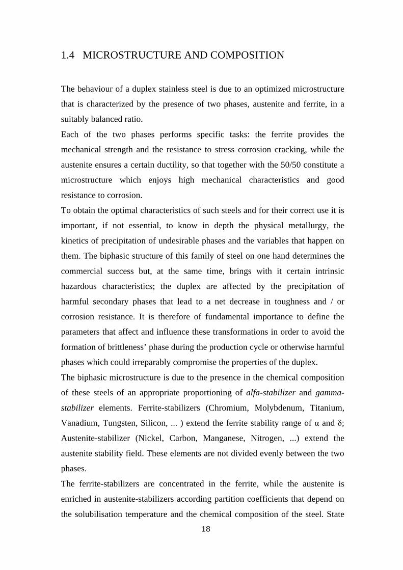
1.4 MICROSTRUCTURE AND COMPOSITION

The behaviour of a duplex stainless steel is due to an optimized microstructure

that is characterized by the presence of two phases, austenite and ferrite, in a

suitably balanced ratio.

Each of the two phases performs specific tasks: the ferrite provides the

mechanical strength and the resistance to stress corrosion cracking, while the

austenite ensures a certain ductility, so that together with the 50/50 constitute a

microstructure which enjoys high mechanical characteristics and good

resistance to corrosion.

To obtain the optimal characteristics of such steels and for their correct use it is

important, if not essential, to know in depth the physical metallurgy, the

kinetics of precipitation of undesirable phases and the variables that happen on

them. The biphasic structure of this family of steel on one hand determines the

commercial success but, at the same time, brings with it certain intrinsic

hazardous characteristics; the duplex are affected by the precipitation of

harmful secondary phases that lead to a net decrease in toughness and / or

corrosion resistance. It is therefore of fundamental importance to define the

parameters that affect and influence these transformations in order to avoid the

formation of brittleness’ phase during the production cycle or otherwise harmful

phases which could irreparably compromise the properties of the duplex.

The biphasic microstructure is due to the presence in the chemical composition

of these steels of an appropriate proportioning of alfa-stabilizer and gamma-

stabilizer elements. Ferrite-stabilizers (Chromium, Molybdenum, Titanium,

Vanadium, Tungsten, Silicon, ... ) extend the ferrite stability range of α and δ;

Austenite-stabilizer (Nickel, Carbon, Manganese, Nitrogen, ...) extend the

austenite stability field. These elements are not divided evenly between the two

phases.

The ferrite-stabilizers are concentrated in the ferrite, while the austenite is

enriched in austenite-stabilizers according partition coefficients that depend on

the solubilisation temperature and the chemical composition of the steel. State

19

diagrams are an essential reference for setting both the working conditions such

as treatment condition to obtain the optimal structure and the use limit

condition.

Unfortunately the composition of the duplex includes 6 or 7 important elements

and is too complex to be described with the usual state diagrams. Therefore we

have to use simplified diagrams as the pseudo-binary diagrams or sections of

the ternary Fe-Cr-Ni diagram.

Schaeffler introduced the concept of Ni and Cr equivalent predicting phase

equilibrium and fields existence of the structures obtained according to the

chemical composition of the alloy. This means that these alloys promote the

formation of ferrite or austenite, so if the ferrite-stabilizer ability is related to

chromium and the austenite-stabilizer is related to nickel it is possible to

measure the total amount of ferrite and austenite stabilizing the effect of this

elements into the steel.

Thanks to the industrial acquired experience, these diagrams were modified to

take account of the different metallurgical states: forged metal, laminate,

welding with or without heat treatment etc.

The values of Ni and Cr equivalent can be calculated using the formula:

Nieq=%Ni+35*%C+20*%N+0,5*%Mn+0,25*%Cu

Creq=%Cr+%Mo+1,5*%Si+0,7*%Nb

The Fig. 3 is used for the previous concept of Nieq e Creq and show the ferrite levels in bands, both as percentages, based on metallographic determinations. [4][9][10]

20

Fig. 3: Schaeffler-Delong diagram with showed the ferrite level in bands as percentage

The pseudo-phase diagrams of DSS are much easier than the ternary. These

charts provide important information on the duplex microstructures and their

evolution, as the temperature changes. Fig. 4 shows that after a primary

solidification in the ferritic phase, the microstructure is partly transformed into

austenitic phase during the subsequent cooling at room temperature.

Fig. 4: State diagram at above 800 ° C. The dotted line refers to the composition of the super duplex

2507.

21

1.5 PHASE TRANSFORMATION Between 300°C and 1100°C duplex stainless steels can present the precipitation

of secondary phases or intermetallic phases that modify their properties. The

“standard” duplex phases (γ and δ) in this temperature range, can lose their

stability, with consequent risk of precipitation due to the fact that some alloy

elements, in particular chromium and molybdenum, tend to migrate from the

solid solution of the matrix to form intermetallic compounds, whose kinetics of

precipitation are most often very slow.

Most of the elements in the alloy tends to broaden the temperature range whose

intermetallic precipitation are likely to increase the rate of formation as shown

in Fig 5. which shows the TTT diagrams for the main types of duplex stainless

steels; it is clear that there are two critical intervals of temperatures in which

there is the formation of secondary phases.

Fig 5: TTT diagram for the most used duplex stainless steel

22

Taking a look again at fig 4 we can see how the austenite, sigma and Cr2N are

consider, for 2507 grade, thermodynamically stable at 800°C.

Anyway, between the range temperature 300-1100°C many secondary phase

can precipitate on the DSS. It possible to identify two main intervals where the

precipitation is stronger.

The first is the “475°C Transformation” where the spinodal decomposition

occurs, which is a demixion of the ferrite in high and poor Cr contents. It’s

possible to notice a subsequent hardening and embrittlement. DSS are sensitive

to this phenomena, that is the reason why most of applications are strictly

restricted to a temperature lower than 250-280°C.

The second interval is between 650-900°C in which the ferrite phase is

thermodynamically unstable. In this range occurs the eutectic decomposition of

the ferrite that decompose into σ-phase and γ’-phase. It has also been observed

a partially precipitation of χ-phase. It is well known that σ-phase precipitate in

all the duplex stainless steel, but this is even more emphasized in the SDSS due

to the high amount of Mo and Cr which move the formation curves of σ-phase

and other phase towards left.

It’s a matter of fact that Mo increase the stability range of the σ-phase to higher

temperature. The σ-phase is brittle and affect the ductility at elevated room

temperature: a small amount of σ-phase reduce heavily the toughness of the

steel even though the tensile properties are not affected to the same extent.

As already seen in Fig 4. the dotted line indicate the DSS 2507 grade, and

following the line we can observe that there is a wide temperature range (950-

1300°C) in which ferrite and austenite are stable together. After 800°C we find

only σ-phase, Cr2N “ε”, and austenite as stable phase.

It is important to notice that the corrosion resistance is a very important

characteristic of this kind of steel, although after the eutectic decomposition of

ferrite we observe a relevant decrease of the corrosion resistance: The presence

of σ-phase decreases resistance to localized corrosion, due to the depletion of

chromium in the surrounding areas of the precipitates σ-phase.

23

It’s already known that if we make a plastic deformation in steel the amount of

internal energy increases, which depends on the rate of deformation. Moreover

after a plastic deformation the tensile strength increases too.

It is quite difficult the analysis for DSS, because their composition is given by

two different phases, one is the ferrite phase (BCC) and the other is the

austenite phase (FCC). The first one is more resistant, has few slip planes and

needs a higher critical stress to activate the first slip plane. In the case of

austenite, it is required a lower activation stress and therefore is easier to

deform.

As written above, σ is a non-magnetic phase with a tetragonal structure. It

normally starts growing at the ferrite boundary and keeps growing into the

grains in a cellular structure form (Fig 6). After that it grows into austenite

grains but slower than into the ferrite grains because the diffusion rate is higher

on the δ-phase.

Fig 6: Diagram of σ-phase nucleation at ferrite/austenite grain boundaries.

There are many articles which have analysed the behaviour of the eutectic

composition in duplex stainless steel, and it has been noticed that previous cold

rolling deformation causes an increase of the rate of ferrite decomposition:

δ à σ + γ’ Previous works have been centred on investigating the effect of plastic

deformation on the precipitation of sigma phase: it has been found that in

24

austenitic steel cold rolled at 20% deformation, cell structure and twins crossing

are kept stable also for temperature of 550°C. [11][12][13]

1.6 APPLICATIONS

Applications of duplex stainless steels are usually those requiring high strength

and excellent corrosion resistance. The typical sectors are mainly oil

production, petrochemicals and desalination plants. DSS are used in oil

production industry thanks to their resistance in conditions of SCC and

localized corrosion [7]. For this reason DSS are frequently used in oil-refinery

heat exchangers where the exposition to chloride-containing process streams,

cooling waters or deposits is consistent.

Fig. 7 Standard duplex 2205 Heat Exchanger pipe Superduplex S32750 are suitable in piping and process equipment for oil/gas

industry. Usually when the corrosive conditions are severe and complex, due to

high chloride concentrations and overheating. Therefore more alloyed DSS are

required to prevent the risk of premature failure.

25

In presence of organic acids, which can cause corrosion problems, duplex and

super duplex, such as S32803 / S32205 and S32750 were found to be suitable

materials for that kind of applications.

Duplex stainless steels are also used in desalination plants[8], but due to the high

costs of alloying elements, like Ni and Mo, that is not the most effective

solution.

Recent statistic data shows that traditional applications as oil and gas, offshore

and petrochemical declines from 27% to 7%.

There is a relative decline also in chemical, storage and transportation, while we

can see increased market share include (waste) water (9% to 18%), construction

and civil engineering (6% to 12%), power generation (1% to 7%) and other

applications[1].

27

CHAPTER 2 EXPERIMENTAL PROCEDURE

The analysed material is the UNS S32750 (SAF2507) Duplex Stainless Steel

the composition has been reported in the table below (Tab 3):

Tab 3. Chemical composition of DSS 2507

2.1 SAMPLE PREPARATION

At the beginning the original bar has been supplied by Outokumpu and was hot

rolled and annealed. This bar has been cut into 35 pieces with this dimensions:

Fig 9. Samples dimensions in mm

Fig 10. Samples after different cold rolled deformation

Once samples were prepared, we cold rolled them in perpendicular direction to

the original grain orientation (to avoid continuous casting weak).

The thickness reduction were: 10% - 20% - 30% - 40% - 50% - 60%

5 out of 35 samples were not cold rolled to be used to compare with the other

deformation samples.

After cold rolling the samples had been heat treated at different temperatures:

700°C – 750°C – 800°C – 850°C for 30 minutes.

28

Due to the big amount of specimens, the table below (Tab 4) explain much better the situation. Cold rolled deformation (%) Heat Treatment Temperature (°C)

0% 10% 20% 30% 40% 50% 60%

20 1 6 11 16 21 26 31

700 2 7 12 17 22 27 32

750 3 8 13 18 23 28 33

800 4 9 14 19 24 29 34

850 5 10 15 20 25 30 35

Tab 4. Specimens table with heat treatment and cold rolled deformation

Once all the samples were heat treated, they were cut into squares 15mm-side

and, to make the handling easier, they were put into a epoxy resin (Fig 11).

Then all the samples has been first grinded with SiC papers starting from P60

up to P2400 and after that for polishing we used clothes with diamond

suspension at 3µ and 1µ.

Fig 11. Specimen embedded in resin

29

Fig 12. Final result after grinding and polishing

30

2.2 OPTICAL MICROSCOPY ANALYSIS The optical microscope was used for the micrographic observation of the

samples. OM technique is usually the first step for metallic materials analysis

and crucial importance is the search for presence of possible precipitating

compounds on the grain boundaries. Moreover this technique can help in

cracks' search, porosity and injuries especially in the samples that has been

heavily cold rolled, and we have seen the dimensional and directional change of

ferrite and austenite grains.

OM technique has two main limits:

• Poor resolving power, less than 0.2 microns.

• Inability to focus on details placed on different levels (field’s depth).

The analysis was performed by Olympus PMG 3 with different magnification

(25x – 50x – 100x – 500x – 1000x) on the two cold rolled directions

(longitudinal and transversal). Photos have been taken for each magnification

and each direction.

After polishing the specimen surface, observed under the microscope, is

specular and it’s impossible to evaluate it. For this reason we have to do a

chemical attack on the specimen surface in order to allow, through a selective

action, differentiation of the various crystalline alloy components and phases.

This chemical attack is called etching. Once the sample was put into the

chemical reagent for less than 20sec, its components will be attacked according

to their reaction rate: the result is the formation of different levels and different

coloration for each component. In other words the surface is no longer specular

but shows the different phases in different colours. The chemical reagent chosen

for the duplex steel 2507 is the Beraha, which the composition is given in Tab

5.

31

Tab 5. Etching composition of Beraha

This chemical attack makes the ferrite phase darker and austenite phase white. [4][9]

During the analysis of the results you have to consider the measurement error. If

you want to give an analytical expression to error bands in the measurements

taken, you can be assessed by standard deviation, denoted by s and defined by

the equation:

𝑠 =𝑥𝑖 − 𝑥𝐴 !!

!!!

𝑛 − 1

where:

- n is the numbers of measurements done

- xi is analysis value

- xA is the average of the values taken defined as

𝑥𝐴 =(𝑥𝑖)𝑛

𝑖=1𝑛

Reagent Chemical composition

Beraha

- 100ml H2O - 20ml HCl - 1g K2S2O5

32

2.3 ELECTRON BACKSCATTER DIFFRACTION (EBSD) Electron Backscatter Diffraction (EBSD) is a microstructural-crystallographic

characterisation technique to study any crystalline or polycrystalline material.

The technique allows us to understanding the structure, crystal orientation and

phase of materials analysed.

EBSD is conducted using a SEM equipped with an EBSD detector. Scanning

Electron Microscope (SEM) is a type of electron microscope that produces

images of a specimen by scanning it with an electron beam. The electrons from

the beam interact with atoms in the sample, producing various signals that give

us information about the sample's surface and composition.

The sample is placed in the SEM and inclined approximately 70o relative to

normal incidence of the electron beam. The detector is a camera equipped with

a phosphor screen (Fig 13). Once the electron beam strikes the sample the

diffracted electrons form a pattern on the phosphor screen which is fluoresced

by electron from the sample to form the diffraction patter.

Fig 13. Scheme of the EBSD technique

33

The phosphor screen is located within the sample chamber of the SEM at an

angle of approximately 90° to the pole piece and is coupled to a compact lens

which focuses the image from the phosphor screen onto the camera. In this

configuration, which electrons which enter the sample backscatter and may

escape. Leaving the sample, electrons may exit at the Bragg condition related to

the crystalline structure and diffract.

These diffracted electrons can escape the material and some will collide and

excite the phosphor screen make it fluorescent.

The specimen is put under high vacuum (10-5 Torr) and has to be conductive

otherwise it produces electrostatic charges which disturb the detection of the

electrons. EBSD allows to analyse the sample at the polished state, without

chemical etching, since the image contrast derives from the different chemical

composition of the phases. In addition the chemical attack, may lead to

difficulties of distinctions of the phases, like precipitates species of small size.

Another advantages of electron microscopy is the chemical analysis of the

microstructural phases.

The image analysis for the determination of the volume fractions of secondary

phases χ and σ is a delicate operation and it depends on the ability of the

operator.

The image analysis stages, after acquisition by SEM, involving the processing

of the image in terms of contrast, illumination and balance to make the

difference between the microstructural phases possible. It follows the step of

segmentation that involves the selection of the grey level of the microstructural

phase to quantify; This is possible thanks to the binarization of the grey scale

for the pixels of the image.

34

2.4 HARDNESS TEST

Hardness is a measure of resistance that quantifies how resistant a solid material

is when a compressive force is applied on it.

For my study has been used KB Prüftechnik with a 200g load. The time load

applied is in a range between 10 and 15 seconds.

Fig. 14 Indentation shape The test consists of measuring the diagonal d of the indentation shape made by

a diamond indenter with a square base. (Fig. 14)

Knowing the applied load (g), we can obtain the value of the Vickers hardness

following the equation:

𝐻𝑉 = 1.854𝑃𝐷 𝐾𝑔𝑚𝑚!

Where P is the load in kg and D is the average length of the diagonal left by the

indenter in millimeters.

35

2.5 X-RAY DIFFRACTION

XRD test has been performed in the University of Miskolc with a Stresstech

Xstress 3000 G3 (Fig 15) which is an accurate and portable X-ray

diffractometer for measuring residual stresses and retained austenite contents.

The machine measures the stresses on crystalline material by Xrays, based on

the phenomenon known as Bragg´s law:

nλ=2dsin(θ)

Fig 15. Xstress 3000 G3 / G3R – Portable X-ray Diffraction (XRD)

36

Where λ is the wavelength of the radiation, d is the distance between two planes

and θ is the scattering angle.

According to the lecture, the crystal lattice is made by atoms that are set

together to form a sequence of parallel planes that divide each other by a

distance d, which depends on the nature of the element.

For a better comprehension on how XRD work follow the Fig 16.

Fig. 16 How the X-Ray can be reflected by the crystal planes[29]

The incoming beam (coming from left) causes each scattered atoms to re-

radiate a small portion of its intensity as a spherical wave. If scattered atoms are

arranged symmetrically with a separation d, these spherical waves will be

synchronized only in directions where their path-length difference 2dsin(θ)

equals an integer multiple of the wavelength λ. In that case, part of the

incoming beam is deflected by an angle 2θ, producing a reflection spot in the

diffraction pattern.[14]

37

The base of the quantitative phase analysis is that Ix,hkl intensity of whichever

X-ray diffraction reflection of a phase is proportional with Vx, where Vx is the

volume of the phase. The formula has been reported here:

𝐼𝑥, ℎ𝑑𝑙 = 𝐶 ∗𝑊 ∗ 𝐻𝑇 ∗ 𝐹 ! ∗ 𝑁! ∗ 𝐴 ∗ 𝐷 ∗ 𝑉𝑥 = 𝐺 ∗ 𝐴 ∗ 𝑉𝑥

where

C is the equipment factor

W is the angle factor and is defined as

𝑊 =1 + cos! 2𝜃𝑐𝑜𝑠𝜃 ∗ sin! 𝜃

where θ is the Bragg angle.

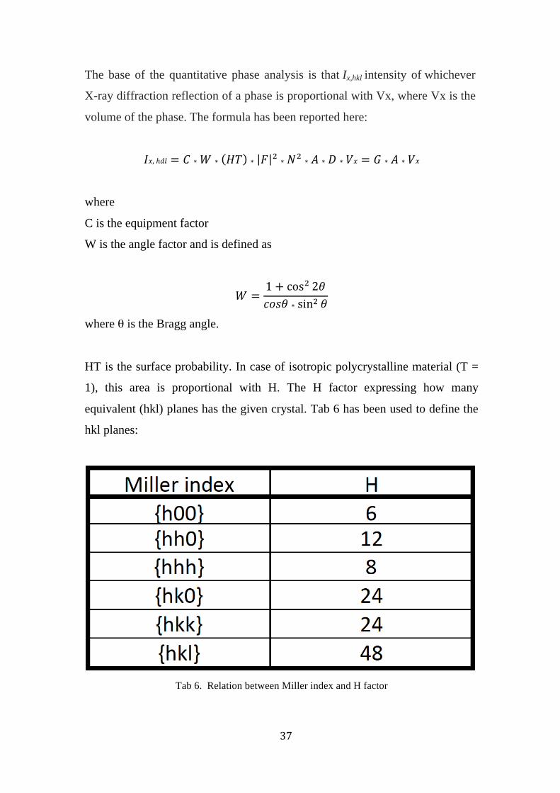
HT is the surface probability. In case of isotropic polycrystalline material (T =

1), this area is proportional with H. The H factor expressing how many

equivalent (hkl) planes has the given crystal. Tab 6 has been used to define the

hkl planes:

Tab 6. Relation between Miller index and H factor

38

N is the unit cell number per unit volume defined as

𝑁 =1𝑎!

where a is the lattice parameter.

A is the absorption factor defined as

𝐴 =12𝜇

where µ is the average mass absorption coefficient, which depends on the

volume ratio of the phases present, that is, what we are looking for.

F2 is a structural factors and has defined as

F(hkl)2 =[f1cos{2π (hi11 + ki12 + li13 )}+ f2cos{2π (hi21 + ki22 + li23 )}+ ... +

fncos{2π (hin1 + kin 2 + lin3 )}]2 + [f1sin{2π (hi11 + ki12 + li13 )} + +f2sin{2π (hi21 + ki22 + li23 )}+ ... + fnsin{2π (hin1 + kin2 + lin3 )}]2

D is the temperature factor (Debye-Waller factor).[18]

39

2.6 MAGNETIC TESTS

Regarding duplex stainless steel, magnetic tests are a valid instrument for

analysis. They can be used to find any kind of variation of ferromagnetic phase

content in the material.

In ferromagnetic materials there isn’t a linear correlation between B and H.

First of all, for equal current, the magnetic field that is produced in them is

much more intense (up to 10 000 times greater). Also a phenomenon called

magnetization saturation occurs whereby the magnetic field no longer increases

once it has reached a certain value for each material. No matter how much

current flows into the solenoid: beyond a certain limit B⃗ stops growing.

The situation is represented by the following figure (Fig 17)

Fig 17. Diagram of magnetic hysteresis loop

40

The hysteresis curve (Fig 17) shows the behaviour of a ferromagnetic material:

it starts at point 0 of the magnetization curve in which the value of B and H is

zero and the material is demagnetised.

If we increase the magnetisation current, I, in a positive direction to some value

the magnetic field strength H increase as well as the flux density B also increase

as shown by the (Fig 17) from 0 to a.

The point b in the hysteresis curve is due to the residual magnetism present in

the material. To lower the flux density at point b to 0 we need to reverse the

current flowing through the coil. The magnetising force which must be applied

to null the residual flux density is called a “Coercive Force”. This coercive

force reverses the magnetic field, re-arranging the molecular magnets until the

core becomes demagnetised at point c.[17]

In this work I have conducted the following magnetic test: Stäblein-Steinitz test,

Eddy-Current test and Fischer-Ferrite test.

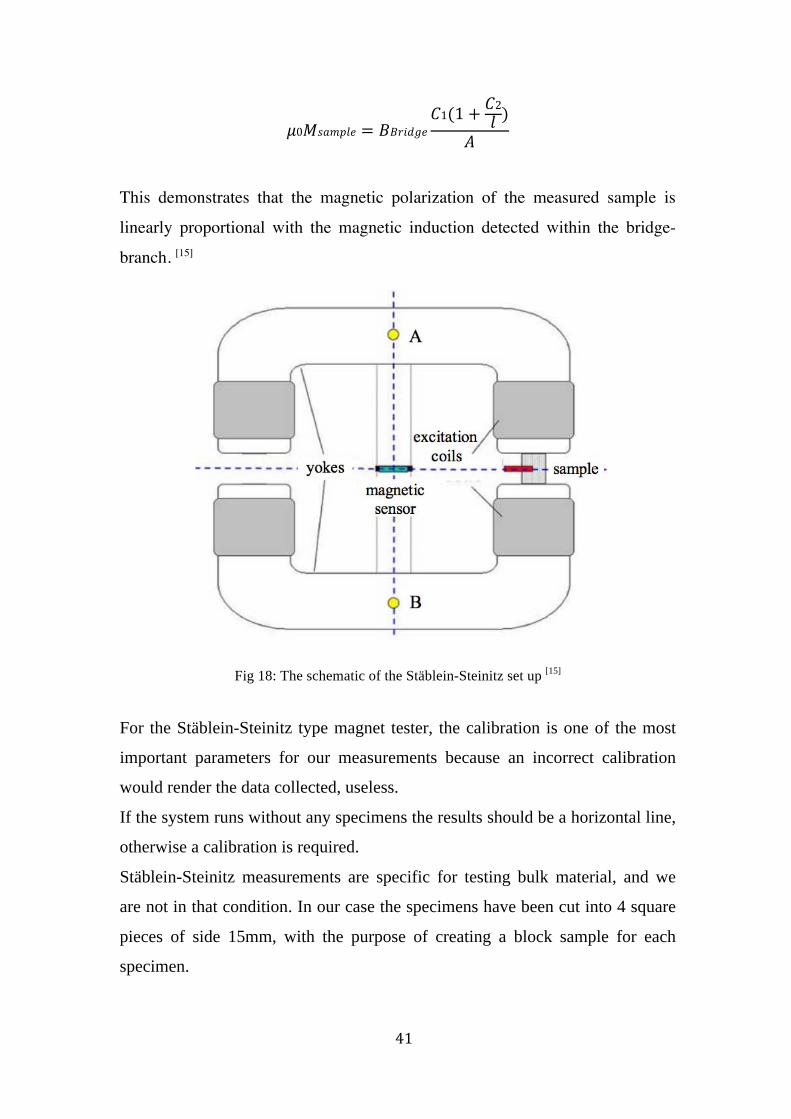
2.6.1 STÄBLEIN-STEINITZ TEST Stäblein-Steinitz tester is a direct current close circuit conceived to reach high

coercivity and magnetization field with specimens that have small dimensions

ratio. It’s based on two iron yokes placed faced each other with an air gap

between the opposite surface (Fig 18)

In both yokes, two excitation coils are placed at the end of each “arm”. There is

a connection between the two yokes so their magnetic fluxes circulate in the

same direction inside the yokes circuit.[26]

If a sample was placed into the measuring air gap it upsets the symmetry of the

yoke and there will be a magnetic flux thought the bridge-branch. The flux of

the bridge-branch can be calculated by a simple concentrated parameter model

of the magnetic circuit. After the proper simplifications it can be derived.

41

𝜇0𝑀𝑠𝑎𝑚𝑝𝑙𝑒 = 𝐵𝐵𝑟𝑖𝑑𝑔𝑒𝐶1(1 + 𝐶2𝑙 )

𝐴

This demonstrates that the magnetic polarization of the measured sample is

linearly proportional with the magnetic induction detected within the bridge-

branch. [15]

Fig 18: The schematic of the Stäblein-Steinitz set up [15]

For the Stäblein-Steinitz type magnet tester, the calibration is one of the most

important parameters for our measurements because an incorrect calibration

would render the data collected, useless.

If the system runs without any specimens the results should be a horizontal line,

otherwise a calibration is required.

Stäblein-Steinitz measurements are specific for testing bulk material, and we

are not in that condition. In our case the specimens have been cut into 4 square

pieces of side 15mm, with the purpose of creating a block sample for each

specimen.

42

We have also calculated the cross section of each block to compare it with the

reference block: the calibration show a proportional relation between the cross

section of the sample and the saturation magnetization value, and thank to the

Stäblein-Steinitz software, knowing the exact specifications of the aluminum

block, took as reference, we can obtain directly the real magnetization value of

the specimens. [4][16][21]

2.6.2 EDDY-CURRENT TEST

Eddy current testing is based on the physics phenomenon of electromagnetic

induction. For a better comprehension look at the Fig 19.

Fig 19. Eddy-Current tester explanation[33]

In an eddy current probe, an alternating current flows through a wire coil at a

chosen frequency and generates an oscillating magnetic field around the coil

(a). When the coil is placed close to an electrically conductive material, like

our duplex steel sample, a circular flow of electrons known as eddy current

will start to move through the metal; in other words eddy current is induced in

the metal (b). That eddy current flowing through the metal will in turn generate

43

its own magnetic field, which will interact with the coil and its field through

mutual inductance. Changes in the sample composition or defects like near-

surface cracking will interrupt or modify the amplitude and pattern of the eddy

current and the resulting magnetic field. This affects the movement of electrons

in the coil by varying the electrical impedance of the coil. With a software is

possible to plots changes in the impedance amplitude and phase angle, which

can be used to identify changes in the test sample.[30]

In this work Eddy-Current test has been done at four different frequency:

10.0KHz – 40.0KHz – 66.7KHz – 100.0KHz

2.6.3 FISCHER-FERRITE TEST

For this work has been used the FERITSCOPE FMP30 by Fischer®, which is

an instrument for measuring the ferrite content in austenitic and duplex steel

according to the magnetic induction method.

Fig 20. Fischer-Ferrite tester explanation

44

The Fischer-Ferrite tester principle is quite simple: a magnetic field generated

by a coil is put in contact with the magnetic component of the specimen. The

variations in the magnetic field lead to a voltage, which is proportional to the

content amount of ferrite in the second coil. Evaluating the voltage we can

obtain the ferrite content.

The FERITSCOPE FMP30 is a portable instrument that can be used to check

the ferrite content in loco, It works with a frequency of 1KHz and it’s powered

by 4x normal R6/LR6 batteries to generate the excitation field required.

This feritscope is an useful instrument for a qualitatively analysis of the ferrite

content.[31]

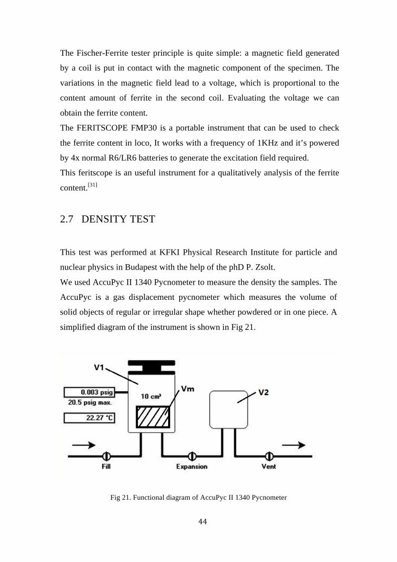
2.7 DENSITY TEST

This test was performed at KFKI Physical Research Institute for particle and

nuclear physics in Budapest with the help of the phD P. Zsolt.

We used AccuPyc II 1340 Pycnometer to measure the density the samples. The

AccuPyc is a gas displacement pycnometer which measures the volume of

solid objects of regular or irregular shape whether powdered or in one piece. A

simplified diagram of the instrument is shown in Fig 21.

Fig 21. Functional diagram of AccuPyc II 1340 Pycnometer

45

Assume that both V1 and V2 are at ambient pressure PA, are at ambient

temperature TA and that the three valves are closed. V1 is then charged to an

elevated pressure P1. The mass balance equation across the sample cell, V1, is

𝑃1 𝑉1 − 𝑉𝑚 = 𝑛𝐶𝑅𝑇𝐴

where

nC = the number of moles of gas in the sample cell

R = the gas constant

TA = the ambient temperature

The mass equation for the expansion volume is

𝑃𝐴𝑉2 = 𝑛𝐸𝑅𝑇𝐴

where

PA = ambient pressure

nE = the number of moles of gas in the expansion volume

When the valves is opened, the pressure falls to an intermediate value, P2, and

the mass balance equation becomes

𝑃2 𝑉1 − 𝑉𝑚 + 𝑉2 = 𝑛𝐶𝑅𝑇𝐴 + 𝑛𝐸𝑅𝑇𝐴

Substituting from the first two equations into the third:

𝑃2 𝑉1 − 𝑉𝑚 + 𝑉2 = 𝑃1 𝑉1 − 𝑉𝑚 + 𝑃𝐴𝑉2

or

𝑃2 − 𝑃1 𝑉1 − 𝑉𝑚 = 𝑃𝐴 − 𝑃2 𝑉2

46

then

𝑉1 − 𝑉𝑚 =𝑃𝐴 − 𝑃2𝑃2 − 𝑃1 𝑉2

Dividing by 𝑃𝐴 − 𝑃2 in both the numerator and denominator we obtain

𝑉𝑚 = 𝑉1 −𝑉2

𝑃1 − 𝑃𝐴𝑃2 − 𝑃𝐴 − 1

Since P1, P2 and PA are expressed in equations as absolute pressures and in the

last equation is arranged so that PA is subtracted from both P1 and P2 before

use, new P1g and P2g may be redefined as gauge pressures

𝑃1𝑔 = 𝑃1 − 𝑃𝐴

𝑃2𝑔 = 𝑃2 − 𝑃𝐴

and we can rewrite the equation as

𝑉𝑚 = 𝑉1 −𝑉2

𝑃1𝑔𝑃2𝑔 − 1

This equation becomes the working equation for the pycnometer. Calibration

procedures are provided to determine V1 and V2 and the pressure are measured

by a gauge pressure transducer. Provisions are made for conveniently charging

and discharging gases at controlled rates, for optimizing the relative sizes of the

sample chamber and expansion volumes, and for cleansing the samples of

vapours.

The gas used by the Accupyc is He because its structure allows it to enter inside

each cavity or porosity of the specimens. [32]

47

2.8 CORROSION TEST

The last test I performed in Budapest was the corrosion test. It consists in

reacting the specimens with a solution of Ferric chloride (FeCl3) for 24, 48 and

72 hours. At the beginning the samples has been cleaned and weighted so that at

the end of the test we can compare the results obtained with the initial ones.

The samples were put in particular supports to increase the amount of surface in

contact with the iron chloride solution (Fig 22).

Fig 22. Specimens put in supports and ready for corrosion test

48

There are two different procedures for the determination of pitting and cervice

corrosion resistant of stainless steels: 1) Method A: Total immersion ferric

chloride test 2) Method B: Ferric chloride cervice test.

The test we performed was the Total immersion ferric chloride test (Method A).

Method A is designed to determine the relative pitting resistance of stainless

steel.

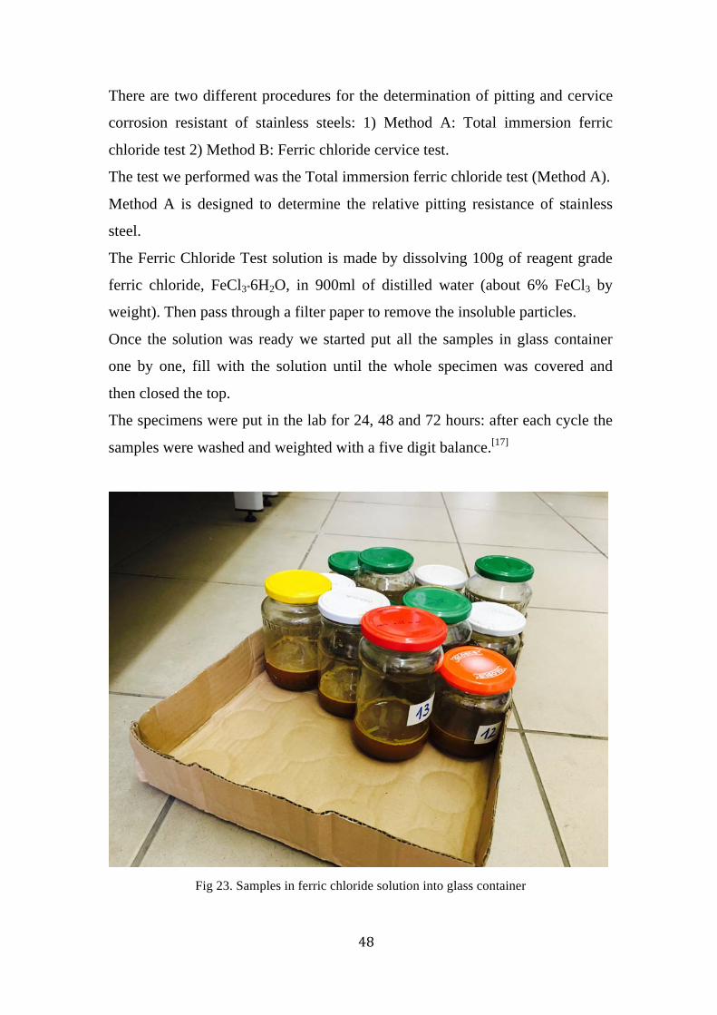
The Ferric Chloride Test solution is made by dissolving 100g of reagent grade

ferric chloride, FeCl3*6H2O, in 900ml of distilled water (about 6% FeCl3 by

weight). Then pass through a filter paper to remove the insoluble particles.

Once the solution was ready we started put all the samples in glass container

one by one, fill with the solution until the whole specimen was covered and

then closed the top.

The specimens were put in the lab for 24, 48 and 72 hours: after each cycle the

samples were washed and weighted with a five digit balance.[17]

Fig 23. Samples in ferric chloride solution into glass container

49

CHAPTER 3 DATA ANALYSIS

3.1 OPTICAL METALLOGRAPHIC ANALYSIS

As explained in chapter 2 all samples have been incorporated into an epoxidic

resin and have been investigated both on the longitudinal and transversal side

according to the cold rolling direction.

The etchant we used for optical metallographic analysis, Beraha, makes ferrite

darker than austenite so we can clearly distinguish between them.

The deformation due to cold rolled has an important effect on the grain’s size

and shape and this fact can be notice along longitudinal direction as stretching

and thinning of austenitic and ferritic grains; different from the transversal

direction effects which is a crushing of both grains.

In our analysis, the reduction size of the grains in 40%, 50% and 60%

deformation samples is significant that only with 50x or more magnification is

possible to distinguish the austenite grains from the ferrite grains.

Therefore the grain’s elongation due to the deformation leads to a chopping of

austenite, which is emphasized with the increase of the deformation.

We noticed that in the samples 1-6-11-16-21-26-31, which are only deformed

without heat treatment, there is no a precipitation of other phases but just a

deformation in the grain boundaries due to the cold rolled.

This phenomena has been also seen in a work regarding 2101 lean duplex

steel.[4]

The following images show the difference between no deformation and 60%

deformation.

50

Fig 24. Base Material without heat treatment and deformation 100x magnification

Fig 25. 60% deformation without heat treatment 100x magnification

51

The main important difference happens on the samples that have been heat

treated: at the temperature of 700°C and 750°C there were not relevant

differences, in the 800°C and 850°C, instead, we can observe a deep

precipitation of sigma phase which amount increase with the deformation.

In the following images sigma phase is shown with a white colour.

1) 2)

3) 4) Fig 26. This 4 images are each one heat treated at 850°C for 1800s, in order

1) No deformation, 2) 20% deformation, 3) 40% deformation 4) 60% deformation

The sigma phase decomposition starts at grain boundaries 1), but some amount

of sigma phase was found inside the austenitic grains 2).

Due to the increase of deformation, most of the ferrite decompose mainly into

sigma phase and in the last two images 3) and 4) there is great difficulty to see

ferrite grains.

In the next page the complete chart can be useful to understand the

decomposition process.

52

3.2 EBSD RESULTS

The EBSD equipment is really useful because gives us much information about

the sample such as phase ratio and grains orientation per each phase detected.

The results from this technique are strongly dependent by the surface’s

condition: if the surface is not perfectly polished by silica clothing, the

instrument can’t analyse the sample properly because the Kikuchi lines[19] were

difficult to detect giving a very low index factor.

We set the equipment with a step distance of 0.3µm between two points inside

the selected area: this procedure took around 2 and 30 minutes to be completed.

Due to the long estimated time we focus our attention in 6 out of 35 samples:

1 5 15 20 25 35

0% | 20°C 0% | 850°C 20% | 850°C 30% | 850°C 40% | 850°C 60% | 850°C

According to the magnetic test, the amount of sigma phase increases in the most

deformed samples.

The images taken by the EBSD instrument were “cleaned up” by the software

choosing 5px as grain size and 5° as degree grain tolerance. The phase map

gives us the phase ratio directly and we can observe it in Tab 6.

Unfortunately the cleaning up process depends on the operators behaviour, and

if the grains are particularly small it’s possible to miss some information.

In Picture 1 we can see clearly just ferrite and austenite because the sample has

not been deformed nor heat-treated. According to the previous results, in

Picture from 2 to 4 we can see how increasing the deformation the amount of

ferrite (red) decrease and decompose into sigma phase (yellow) and secondary

austenite (green).

In the following images we can see the analysed phase map by EBSD:

53

Picture 1. Base material, sample number 1

Picture 2. Sample number 5 heat treated at 850°C without deformation

54

Picture 3. Sample number 25 (40% - 800°C)

Picture 4. Sample number 35 (60% - 850°C)

55

In the following table we can see the trend of the sigma-phase with the

deformation rate. The huge precipitation of sigma is substantial and in the last

sample (number 35), most of ferrite has been decomposed. The phase ratio can be observed in the following table:

SAMPLE Ferrite Austenite Sigma-‐phase

1 41% 59% 0%

5 34,90% 57,60% 7,50%

15 33,20% 53,80% 13,00%

20 8,70% 72,90% 18,40%

25 9,80% 68,40% 21,80%

35 1,30% 52,30% 46,40% Tab 6. Percentage of phase content in different sample with EBSD investigation

56

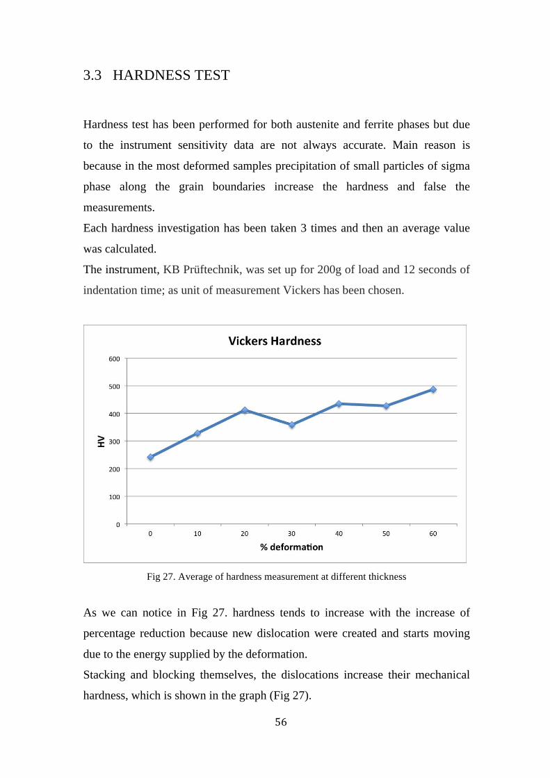
3.3 HARDNESS TEST

Hardness test has been performed for both austenite and ferrite phases but due

to the instrument sensitivity data are not always accurate. Main reason is

because in the most deformed samples precipitation of small particles of sigma

phase along the grain boundaries increase the hardness and false the

measurements.

Each hardness investigation has been taken 3 times and then an average value

was calculated.

The instrument, KB Prüftechnik, was set up for 200g of load and 12 seconds of

indentation time; as unit of measurement Vickers has been chosen.

Fig 27. Average of hardness measurement at different thickness

As we can notice in Fig 27. hardness tends to increase with the increase of

percentage reduction because new dislocation were created and starts moving

due to the energy supplied by the deformation.

Stacking and blocking themselves, the dislocations increase their mechanical

hardness, which is shown in the graph (Fig 27).

57

The information we got from this test is purely qualitatively because they are

about the surface of the specimen and we cannot investigate inside the sample

itself.

We also focused on hardness variation due to both the heat treatment and the

thickness reduction and we the results can be seen in the Fig 28.

Fig 28. Hardness variation due to different heat treatment and deformation

As we can see, the hardness significantly increases in all samples starting from

750 °C. It is also possible to notice that the effect due to the deformation moves

upwards the curves gradually due to deformation increase.

This increase over 750°C is due to the high amount of sigma phase precipitated

in the samples, which is hard and brittle.

58

3.4 STÄBLEIN-STEINITZ TEST

In previous work on duplex stainless steel 2507[16], AC measurements test

weren’t able to supply an excitation field high enough to saturate 2507 DSS.

That’s the reason why we used DC measurements like Stäblein-Steinitz tester: it

can reach over 3000A/cm, which is greater than AC measurement test.

In the following images we can see the hysteresis loop of deformed samples

without heat treatment:

a)

b)

59

c)

Fig 29. Hysteresis loop of a) 0% thickness reduction b) 20% thickness reduction and c) 40%

thickness reduction at room temperature

Although the curves do not have the same origin, the hysteresis curves are

almost equal, and for this reason we have confirmation that the different

thickness reduction do not influence the amount of ferromagnetic phase in the

steel.

The shift of the curves from the origin is due to the device’s calibration, which

should be done for each samples making this measurements extremely long.

The Stäblein-Steinitz tester without samples should show an horizontal line, but

it didn’t happen due to error of the instrument so we analysed the “horizontal

line” found out that the slope increase of the order of 1.2*10-5 and so we

adjusted each curves with that factor.

Moreover we calculated for each graph the saturation polarization value BSP

subtract the minimum value of the loop to the maximum and divided the result

by two.

𝐵𝑆𝑃 =𝑀𝐴𝑋 −𝑀𝐼𝑁

2

60

We put all the BSP in a graph for a better comprehension:

Fig 30. Saturation polarization diagram for each thickness reduction

The graph in Fig 30 shows the trend of the saturation polarization value. Except

for one point in 10% thickness reduction sample at 800°C which is due to

operator or instrument error, others show a decrease in heat treated samples at

temperature higher than 750°C.

In this samples the amount of ferromagnetic phase, so called ferrite, is

extremely low due to the decomposition process into sigma phase and

secondary austenite, this is the reason why the saturation polarization value

decreased.

More deformed is the specimen, lower is the ferrite content and lower is the

saturation polarization value.

61

3.5 EDDY-CURRENT TEST

Each specimen has been measured at 4 different frequencies: 10kHz – 40kHz –

66,7kHz – 100kHz.

62

Fig 31. 4 frequencies diagrams of Eddy-Current test

The four graphs show the amount of ferrite calculated at different frequencies,

we notice that the 10kHz measurement is the most accurate ones according to

the EBSD results.

63

3.6 FISCHER-FERRITE TEST

Before the test all samples has been polished by 320P to remove every possible

oxide substrate on the surface, which would distort the measurements.

The measures were taken for each face of the specimen and in the following

table the data is an average of 4 measurements of the same face.

T (°C) e=0% e=10% e=20% e=30% e=40% e=50% e=60% 20 47,4 45,7 42,5 42,1 41 39,7 38,9 700 41,2 38,7 38,2 37,2 39,1 37,4 35 750 37,6 37 36,9 37 37,3 35,3 34,4 800 35,4 33,4 32,5 31,1 22,3 13,7 7,8 850 27,8 25,4 15,7 9,3 5,5 2,6 1,4

Tab 7. Ferrite percentage measured with Fischer feritscope

For a better analysis we had inserted all the data collected into a graph:

Fig 32. Ferrite content calculated with Fischer-Feritscope at different heat treated samples

We can observe that, according to the Eddy-Current and Stäblein-Steinitz test,

the amount of ferrite decrease with heat treatment over 750°C.

64

3.7 X-RAY DIFFRACTION TEST

Samples were investigated in the Metallurgy Institute at University of Miskolc.

Tab 8 shows those samples which have been investigated by X-ray diffraction.

Tab 8. Investigated samples by XRD

The diffractograms were created by a D8 Advanced diffractrometer with

copper X-ray radiation. Qualitative phase analysis was made by Bruker EVA

software and was determined by APX63 software. Two samples out of 6 were

measured in parallel with Göbel mirror and Bruker D8 Advanced equipment

(which contained a position sensitive detector) in the Mineralogy Institute at

the University Of Miskolc. Rietveld method and Bruker Topas software were

used on the diffractograms to determine the amount of the phases.

Unfortunately the results obtained by APX63 software are completely wrong

and they were not included in this thesis.

At least 3 reflections of a phase need for the program to calculate the content

amount of the phase. If there is less reflection the matrix, which is necessary

for the calculation, cannot exist.

Sample

number

Deformation

rate (%)

Heat

Treatment

Temperature

(°C)

Ferrite

(%)

Austenite

(%)

Sigma

(%)

1 0 20 42.31 57.69 -

35 60 850 - 54.45 45.55

Tab 10. Ferrite, Austenite and Sigma percentage results with Rietveld method

Sample number Deformation rate (%) Heat Treatment Temperature (°C) Fig. 1 0 20 1,2,6 3 0 750 2,3 5 0 850 2,5 20 30 850 5 33 60 750 3,4 35 60 850 1,4,7

65

We noticed that there are differences between the Rietveld method results (Tab

10) and the other results (Tab 9).

The possible reasons of this differences:

• The texture of the sample, for example: in sample 1, the orientation

which was considered by the ferrite first refection could not be used by

the second reflection

• There is no proper crystallography information about the dissolved Cr

atoms in case of the sigma-FeCr phase: in sample 35, 5% Cr was

supposed but if the solubility is higher it can cause significant changes.

For this reason we do not take into consideration the results from Tab 9. and

we analysed only results from Tab 10.

The Fig 33 shows the diffractogram of sample 1, which contained only ferrite

and austenite.

Fig 33. Diffractogram of sample 1, blue curve is ferrite content, orange curve is austenite

66

The sample number 35, which was 60% cold rolled and heat treated at 850°C,

contained largely austenite and sigma phase and can be confirmed by Fig 34.

Fig 34. Diffractogram of sample 35, green curve is sigma content, grey curve is austenite

According to EBSD results, the Rietveld method results are quite good.

Unfortunately this test takes from 7 to 8 hours to be completed for one sample

and only two samples had been evaluated.

67

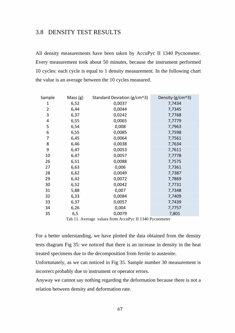
3.8 DENSITY TEST RESULTS

All density measurements have been taken by AccuPyc II 1340 Pycnometer.

Every measurement took about 50 minutes, because the instrument performed

10 cycles: each cycle is equal to 1 density measurement. In the following chart

the value is an average between the 10 cycles measured.

Sample Mass (g) Standard Deviation (g/cm^3) Density (g/cm^3) 1 6,52 0,0037 7,7434 2 6,44 0,0044 7,7345 3 6,37 0,0242 7,7768 4 6,55 0,0065 7,7779 5 6,54 0,008 7,7963 6 6,55 0,0085 7,7598 7 6,45 0,0064 7,7561 8 6,46 0,0038 7,7634 9 6,47 0,0053 7,7611 10 6,47 0,0057 7,7778 26 6,51 0,0088 7,7575 27 6,63 0,006 7,7361 28 6,62 0,0049 7,7387 29 6,42 0,0072 7,7869 30 6,52 0,0042 7,7731 31 5,88 0,007 7,7348 32 6,33 0,0084 7,7409 33 6,37 0,0057 7,7439 34 6,26 0,004 7,7757 35 6,5 0,0079 7,801

Tab 11. Average values from AccuPyc II 1340 Pycnometer

For a better understanding, we have plotted the data obtained from the density

tests diagram Fig 35: we noticed that there is an increase in density in the heat

treated specimens due to the decomposition from ferrite to austenite.

Unfortunately, as we can noticed in Fig 35. Sample number 30 measurement is

incorrect probably due to instrument or operator errors.

Anyway we cannot say nothing regarding the deformation because there is not a

relation between density and deformation rate.

68

Fig 35. Density test data plotted in a graph

3.9 CORROSION TEST RESULTS

After 24h all samples had been cleaned from ferric chloride and weighed, and

this procedure has been repeated after 48h and 72h.

First of all, the specimens with the highest heat treatment were heavily damaged

and this can be observed easily to the naked eye.

A table with all the masses before and after the 24h, 48h and 72h had been

prepared (Tab 12) and after that a graph had been plotted to analyzed the mass

variations of the samples.

69

Tab 12. Mass reduction after 24h, 48h and 72h

Original mass (g)

Mass after 24h

(g)

Mass after 48h

(g)

Mass after 72h

(g) Mass reduction after 72h (g)

Mass reduction

after 72 h (%) 1 6,518 6,5176 6,5175 6,5170 0,0010 0,015342129 2 6,4373 6,4365 6,4363 6,4361 0,0012 0,018641356 3 6,3644 6,3639 6,363 6,3626 0,0018 0,02828232 4 6,5302 6,5254 6,5219 6,5078 0,0224 0,343021653 5 6,5208 6,4462 6,4406 6,4397 0,0811 1,243712428 6 6,5396 6,5395 6,5395 6,5395 0,0001 0,001529146 7 6,4271 6,4262 6,4258 6,4248 0,0023 0,035785969 8 6,438 6,4375 6,4369 6,4365 0,0015 0,023299161 9 6,4648 6,464 6,4631 6,4627 0,0021 0,032483604 10 6,4468 6,4208 6,4168 6,4139 0,0329 0,510330707 11 6,1098 6,1096 6,1083 6,1083 0,0015 0,024550722 12 5,9583 5,9582 5,9582 5,958 0,0003 0,005034993 13 6,6411 6,6405 6,6402 6,6399 0,0012 0,018069296 14 6,5735 6,5707 6,5694 6,5678 0,0057 0,086711797 15 6,4182 6,2442 6,2298 6,2268 0,1914 2,982144527 16 6,2033 6,2032 6,2031 6,203 0,0003 0,004836136 17 6,3423 6,3421 6,342 6,3409 0,0014 0,022074011 18 6,6548 6,6538 6,6535 6,6535 0,0013 0,019534772 19 6,4051 6,3867 6,3784 6,377 0,0281 0,438712901 20 6,4373 6,3139 6,2434 6,223 0,2143 3,329035465 21 6,4936 6,4933 6,4931 6,493 0,0006 0,009239867 22 6,373 6,3729 6,3728 6,3728 0,0002 0,003138239 23 6,6259 6,6257 6,6255 6,6252 0,0007 0,010564603 24 6,4919 6,2448 6,163 6,1525 0,3394 5,22805342 25 6,7338 6,5045 6,4163 6,3977 0,3361 4,991238231 26 6,495 6,4949 6,494 6,4938 0,0012 0,018475751 27 6,6284 6,628 6,627 6,6269 0,0015 0,022629896 28 6,614 6,6138 6,6137 6,6135 0,0005 0,007559722 29 6,3945 6,0665 6,0152 5,9998 0,3947 6,172491985 30 6,5252 6,239 6,1482 6,1368 0,3884 5,952307975 31 5,8656 5,8655 5,8654 5,8654 0,0002 0,003409711 32 6,3095 6,3089 6,3082 6,3081 0,0014 0,022188763 33 6,3584 6,358 6,3579 6,3578 0,0006 0,009436336 34 6,255 6,0244 5,9924 5,9582 0,2968 4,745003997 35 6,4799 6,3205 6,258 6,2448 0,2351 3,62814241

70

Fig 36. Mass reduction after 72h

Looking at Fig 36, we can say that under 750°C the mass reduction is very low,

practically we can’t see a reduction, because the ferrite phase didn’t transform

into sigma phase and secondary austenite. The corrosion resistance decrease

above 750°C, due to the decomposition of ferrite and this results are similar to

the DC magnetometer results, because the mass reduction starts where the

eutectoid decomposition begins (which is over 750°C).

We also counted the number of pittings, which were formed at the end of each

corrosion cycle. But there isn’t a correlation between the pitting number and the

deformation.

Fig 37. Number of pittings after 72h

71

Fig 38. Sample number 29 before the corrosion test.

Fig 39. Sample number 29 after 72h into FeCl3

73

CONCLUSIONS

The DSS 2507 type was investigated by different magnetic tests like Stäblein-

Steinitz. Eddy-Current and Fischer ferrite but also with non-destructive tests

like EBSD and Density test and destructive tests like hardness and corrosion

test.

We analysed the decomposition process of δ-ferrite phase due to heat treatment

and cold rolling deformation and see the relation between them in the process.

We noticed that:

• The phase transformation starts between the range of 700°C and 750°C

and, according to the tests, the rate of the phase transformation increases

with the deformation.

• In the non deformed samples (1 to 5) the phase transformation starts at

the grain boundaries, in the deformed samples the decomposition occurs

inside the grain boundaries as well.

• The σ-phase precipitation is enhanced by the plastic deformation, and in

the most deformed sample (50% and 60%) the ferrite had almost

completely disappeared.

• Hardness test shows that hardness increase due to plastic deformation.

At 800°C, in strongly deformed samples, the increase of σ-phase amount

leads to an increase of hardness.

74

• As noticed in the density test, between 700°C-750°C there is an increase

of specific density of the alloy due to the reduction of ferrite (lower

density) compared to austenite (higher density).

• Analysing the corrosion test we can confirm that the optimal ratio of

ferrite and austenite in DSS for the best corrosion resistance is 45%

ferrite and 55% austenite: if the amount of ferrite decrease even just 5%

corrosion has detected.

75

REFERENCE:

[1] E.C. Bain, W.E. Griffith, Trans AIME, 75 (1927) 166.

[2] R.N. Gunn, Duplex Stainless Steels: Microstructure, properties and

applications. Ed.

[3] I. Alvarez-Armas, Duplex Stainless Steels: Brief History and Some

Recent Alloys, Recent Patents on Mechanical Engineering, 1 (2008)

51-57.

[4] Giovanni Fassina, Effects of cold rolling on austenite to α ’ - martensite

transformation in 2101 lean duplex stainless steel, Msc work, 2010.

[5] R.N. Gunn, Duplex Stainless Steels: Microstructure, properties and

applications. Ed.

[6] I. Alvarez-Armas, Duplex Stainless Steels: Brief History and Some

Recent Alloys, Recent Patents on Mechanical Engineering, 1 (2008)

51-57.

[7] D.S. Bergstrom, Benchmarking of Duplex Stainless Steels versus

Conventional Stainless Steel Grades, Proc. 7th Duplex 2007 Int. Conf

& Expo, Grado, Italy (2007).

[8] J. Olsson, M. Snis, Duplex - A new generation of stainless steels for

desalination plants. Desalination, 205 (2007) 1-3: 104-113.

[9] Manfrin, Effetto della deformazione a freddo sulle trasformazioni di

fase per l’acciaio SAF2507 indotte da trattamento termico, Msc work,

2011.

[10] Bela Leffler, Stainless steels and their properties, Outokumpu

publication.

[11] Gomes de Abreu, Santana de Carvalho, de Lima Neto, Pires dos

Santos, Nogueira Freire, de oliveira silva, souto mario tavares.

Deformation Induced Martensite in an AISI 301LN Stainless Steel:

Characterization and Influence on Pitting Corrosion Resistance,

Materials Research, Vol. 10, No. 4, (2007) pp 359-366.

[12] Weisbrodt-Reisch, Brummer, Hadler, Wolbank, Werner, Influence of

76

temperature, cold deformation and a constant mechanical load on the

microstructural stability of a nitrogen alloyed duplex stainless steel.

Materials Science and Engineering A 416 (2006) pp 1–10.

[13] Hadji, Badji, Microstructure and Mechanical Properties of Austenitic

Stainless Steels After Cold Rolling, JMEPEG (2002) 11 pp 145-151.

[14] Stablein, F. – Steinitz, R.: Ein Neuer Doppeljoch Magnetstalprüfer,

Archiv für das Eisenhüttenwesen 8, (1935), 549-554.

[15] I. Mészáros, Testing of stainless steel by double yoke DC

magnetometer Journal of electrical engineering, VOL 61. NO 7/s, 2010,

62-65

[16] Bianchi M. Effects of cold rolling on phase precipitation and phase

transformation in a 2507 SDSS Msc work (2011)

[17] ANSI/ASTM G48 Pitting and crevice corrosion resistance of stainless

steels and related alloys by the use of ferric chloride solution, 1976

[18] D O’Sullivan, M Cotterell, D A Tanner, I Mészáros: Characterisation

of ferritic stainless steel by Barkhausen techniques, NONDESTRUCT

TEST EVA 37: 489-496 (2004)

[19] Tibor Berecz, István Mészáros: Studying of Microstructural Effects of

Surface Rolling in Materials of Railway-car Wheel Axles by EBSD and

NDT Magnetic Measurement, MATER SCI FORUM 729: 308-313

(2013)

[20] I Calliari, M Breda, E Ramous, I Mészáros: Phase transformations in

duplex stainless steels: Metallographic and magnetic investigation,

YEJIN FENXI 33: (7) 10-15 (2013)

[21] S Baldo, I Mészáros: Effect of cold rolling on microstructure and

magnetic properties in a metastable lean duplex stainless steel, J

MATER SCI 45: 5339-5346 (2010)

[22] M Breda, L Pezzato, M Pizzo, I Mészáros, I Calliari: Effects of Cold

Deformation in Duplex Stainless Steels, In: EUROMAT 2013.

77

[23] Weisbrodt-Reisch, Brummer, Hadler, Wolbank, Werner, Influence of

temperature, cold deformation and a constant mechanical load on the

microstructural stability of a nitrogen alloyed duplex stainless steel.

Materials Science and Engineering A 416 (2006) pp 1–10.

[24] Maitlan, Sitzman, Electron Backscatter Diffraction (EBSD) Technique

and Materials Characterization Examples, Scanning microscopy for

nanotechnology techniques and applications (2007) pp 41-75.

[25] Tibor Berecz, István Mészáros, Péter János Szabó: Decomposition of

the Ferritic Phase in Isothermally Aged SAF 2507 Duplex Stainless

Steel, MATER SCI FORUM 589: 185-190 (2008)

[26] I Mészáros: Magnetic characterisation of duplex stainless steel,

PHYSICA B 372: 181-184 (2006)

[27] S Baldo, M Zanelatto, I Mészáros: Phase transformation in 2101 DSS

after cold rolling, In: DUPLEX Stainless Steels 2010: DUPLEX 2010

AIME, 2010. pp. 10 (Konferenciaközlemény)

[28] B. Bögre, I. Mészáros – Study of ferrite decomposition in duplex

stainless steel Volume 66, 2015. December ISSN 1335-3632 (4 oldalas

cikk)

[29] https://en.wikipedia.org/wiki/X-ray_crystallography

[30] http://www.electronics-tutorials.ws/electromagnetism/

[31] http://www.helmut-fischer.ch/

[32] http://www.rmki.kfki.hu/

[33] http://www.olympus-ims.com/en/eddycurrenttesting/

effects of heat treatment and cold rolling on …

Documents