effects of climate variability on the carbon dioxide, water, and

Agricultural and Forest Meteorology 101 (2000) 113–129

Effects of climate variability on the carbon dioxide, water, and sensibleheat fluxes above a ponderosa pine plantation in the Sierra Nevada (CA)

A.H. Goldsteina,∗, N.E. Hultmana,c, J.M. Frachebouda, M.R. Bauera, J.A. Paneka,M. Xu a, Y. Qi a, A.B. Guentherb, W. Baughb

a Department of Environmental Science, Policy and Management, University of California, 151 Hilgard Hall, Berkeley 94720-3110, USAb Atmospheric Chemistry Division, National Center for Atmospheric Research, Boulder, CO, USA

c Energy& Resources Group, University of California, Berkeley, USA

Received 1 April 1999; received in revised form 2 December 1999; accepted 3 December 1999

Abstract

Fluxes of CO2, water vapor, and sensible heat were measured by the eddy covariance method above a young ponderosa pineplantation in the Sierra Nevada Mountains (CA) over two growing seasons (1 June–10 September 1997 and 1 May–30 October1998). The Mediterranean-type climate of California is characterized by a protracted summer drought, with precipitationoccurring mainly from October through May. While drought stress increased continuously over both summer growing seasons,1998 was wetter and cooler than average due to El Niño climate patterns and 1997 was hotter and drier than average. Oneextreme 3-day heat wave in 1997 (Days 218–221) caused a step change in the relationship between H2O flux and vaporpressure deficit, resulting in a change in canopy conductance, possibly due to cavitation of the tree xylem. This step changewas also correlated with decreased rates of C sequestration and evapotranspiration; we estimate that this extreme climaticevent decreased gross ecosystem production (GEP) by roughly 20% (4mmol C m−2 s−1) for the rest of the growing season. Incontrast, a cooler, wetter spring in 1998 delayed the onset of photosynthesis by about 3 weeks, resulting in roughly 20% lowerGEP relative to the spring of 1997. We conclude that the net C balance of Mediterranean-climate pine ecosystems is sensitiveto extreme events under low soil moisture conditions and could be altered by slight changes in the climate or hydrologicregime. ©2000 Elsevier Science B.V. All rights reserved.

Keywords:Net ecosystem exchange; Climate variability; Ponderosa pine; Eddy covariance

1. Introduction

Forests play an important role in the exchange ofcarbon, water and energy between the land and theatmosphere. As a major store of mobilizable carbon,they can strongly influence the global carbon cycleand thus climate (Musselman and Fox, 1991). Under-standing the dynamics of carbon exchange between

∗ Corresponding author. Tel.:+1-510-643-2451;fax: +1-510-643-5098.E-mail address:[email protected] (A.H. Goldstein).

the atmosphere and the forested biosphere has beenthe goal of recent ecosystem-scale projects, manyof which are now part of the Ameriflux or Eurofluxnetworks. These projects study biomes that are rep-resentative of large areas of the terrestrial biosphere,such as boreal forest (BOREAS, e.g. Margolis andRyan, 1997), temperate broad-leafed deciduous for-est (Wofsy et al., 1993; Baldocchi, 1997), southeastconiferous forest (Clark et al., 1999), and tropicalforest (Grace et al., 1995). The carbon sequestrationrate for most of these ecosystems is controlled bylight availability and timing of new leaf development

0168-1923/00/$ – see front matter ©2000 Elsevier Science B.V. All rights reserved.PII: S0168-1923(99)00168-9

114 A.H. Goldstein et al. / Agricultural and Forest Meteorology 101 (2000) 113–129

(e.g. Goulden et al., 1996), among other factors; alimited number of canopy-scale eddy covariance stud-ies have shown that drought stress can also play asignificant role in net ecosystem exchange (e.g. Bal-docchi, 1997). While the Mediterranean zonobiome(including California) is a significant biome globally,little attention has been given to canopy-scale forestresponses to this climate. Furthermore, although pon-derosa pine (Pinus ponderosaDoug. ex. Laws) is themost common conifer species in North America, thisforest type has only recently been investigated by suchcanopy scale studies (Anthoni et al., 1999; Baldocchiet al., 2000; Law et al., 1999a, b, 2000a ). Finally, re-cent forest management in many parts of the US hasresulted in millions of acres of young, growing forest.Of the US Forest Service land in the Sierra Nevada,380,000 acres (4%) is in plantation, and 34% of thatis ponderosa pine plantation (Landram, 1996). Theseeven-aged stands provide an excellent opportunity toinvestigate the capacity of a young, managed forest tosequester carbon under drought-stressed conditions.

Winter precipitation (October–May) and summerdrought characterize the Mediterranean-type climateof California. Freezing temperatures limit growth inthe early spring, and low soil moisture and high va-por pressure deficits (VPD) limit growth in the latesummer. This climate thus imposes hydrologic andtemperature limitations to ecosystem gas and energyexchange during summer months.

To examine the effects of interannual climatevariability on canopy-scale carbon, water, and en-ergy fluxes, we established a measurement site in ayoung ponderosa pine plantation in the Sierra NevadaMountains of California and observed forest responseduring natural variations of climatic conditions. Wepresent data acquired continuously over two climati-cally different growing seasons: 1997 was drier thanthe climatic mean, and 1998 was cooler and wetterthan the climatic mean (influenced by El Niño).

2. Materials and methods

2.1. Site description

The field site was established in May 1997 in aponderosa pine plantation, owned and operated by

Sierra Pacific Industries. The plantation is located(3853′42.9′′N, 12037′57.9′′W, 1315 m) adjacent toBlodgett Forest Research Station, a research forest ofthe University of California, Berkeley (Fig. 1).

The forest constituting the sampled daytime ‘foot-print’ of the tower was a 4 m homogenous canopyof 6–7-year-old trees dominated by ponderosa pine.The canopy also included individuals of Douglasfir (Pseudotsuga menziesii), white fir (Abies con-color), giant sequoia (Sequoiadendron giganteum),incense-cedar (Calocedrus decurrens) and Californiablack oak (Quercus kelloggii). The major understoryshrubs were manzanita (Arctostaphylosspp.) andCeonothusspp. In 1997, about 25% of the groundarea was covered by shrubs, 30% by conifer trees,2% by deciduous trees, 7% by forbs, 3% by grassand 3% by stumps. Two separate model estimates ofthe tower footprint agreed that roughly 90% of thefootprint was within the young plantation (200 m ofthe tower) during the daytime (lagrangian stochasticdispersion model by Hsieh et al., 1997, results pro-vided by Hsieh; eulerian advection-diffusion modelby Horst and Weil, 1994, results reported in Bakeret al., 1999). This footprint area was in a stage ofrapid growth, as exhibited by the large (30–35%)increase in leaf area index (LAI) between the 1997and 1998 growing seasons (Table 1). Two hundredmeters upwind (daytime) of the measurement site, thecanopy foliar density increased sharply; the transi-tion reflected the borderline between the 6–7-year-oldplantation and a 12–13-year-old plantation southwestof the measurement site. The predominant daytimeairmass trajectory at the site is directed upslopefrom the Sacramento Valley (from the southwest,210–240). At night, air flows downslope from theSierra Nevada Mountains (from the northeast,∼30).The site was relatively flat. The slope of terrain within

Table 1Ecosystem total LAI (m2 leaf per m2 ground area)a

Initial Maximum Final

1997 LAI 3.9 6.6 5.31998 LAI 5.3 9.0 7.1Ratio 1.4 1.4 1.3

a LAI includes tree and shrub leaf area. Initial indicates LAIbefore budbreak, and final indicates LAI after loss of third yearneedles. Two age classes of needles were typically retained throughthe winter. Uncertainty in LAI estimates is approximately 20%.

A.H. Goldstein et al. / Agricultural and Forest Meteorology 101 (2000) 113–129 115

Fig. 1. Index map showing the regional setting and details of the Blodgett Forest tower site. The upper image shows regional vegetation.It is derived from the USGS Seasonal Land Cover Regions classification, which is based on 1 km pixel AVHRR data. The ‘Oak Forests’category shown here comprises both oak forest and woodland areas. The lower image shows details of the tower site and is based on aUSGS 3.75 min digital orthophoto quadrangle with 1 m pixels.

200 m of the tower varied less than 2 in the north,east, and south but was 0–15 to the west where acreek flows from south to north. The slopes beyond200 m but within 1000 m of the site were larger andvaried from 0–15, 0–10, 0–5, and 0–30 in the north,east, south, and west, respectively.

The site is characterized by a Mediterranean cli-mate (Table 2). Since 1961, annual precipitation hasaveraged 163 cm (254 cm snow), with the majority of

precipitation falling between September and May, andalmost no rain in the summer. Summer temperatureaverages range from 14–27C (daily low to daily high)and winter temperatures from 0–9C (data from Blod-gett Forest archives, F. Schurr). Trees generally breakbud in May and set bud in late July to early August;1998 was an exception, with the start of needle elon-gation delayed until late June. Predawn water potentialin ponderosa pine can be expected to drop as low as


Table 2Rainfall and climate comparisona

1997 1998

February–May rainfall 18 cm 117 cm% of normal February–May rainfall 27% 176%Last subzero day Day 121 Day 146Bud break Day 145 Day 180

a The 1997 February–May rainfall was 27% of normal (averagesince 1961); in 1998 the rainfall was 176% of normal. The lastfrost and bud break were delayed by approximately 1 month in1998.

−1.0 MPa by the end of the growing season (based onobservations of 12-year-old ponderosa pine at a site2 km upwind of the tower throughout the 1997 grow-ing season).

The soil is a fine-loamy, mixed, mesic, ultic hap-loxeralf in the Cohasset series whose parent materialwas andesitic lahar. It is relatively uniform, comprisedpredominantly of loam or clay-loam. Cohasset soilsare inherently very porous (up to 65% by volume)primarily due to the high proportion of fine particles(L. Paz, personal communication). The top 30 cm ofsoil in 1998 contained 6.9% organic matter and 0.17%nitrogen.

Infrastructure for the canopy scale flux measure-ments included a 10 m measurement tower (UprightInc.), a temperature-controlled instrument building,and an electrical generation system powered by a30 kW diesel generator (Kohler). The measurementtower was placed towards the eastern end of the standto maximize the ponderosa pine plantation fetchduring the day. The generator was located 130 mnorthwest of the tower, as far outside of the majorairflow paths as possible. Hydrocarbon measurementsat the site indicated that exhaust from the generatoraffected our measurements less than 5% of the time,and contamination occurred only at night (Lamannaand Goldstein, 1999).

2.2. Measurements and calculations

From 1 June to 10 September 1997 and from 1 Mayto 30 October 1998, fluxes of CO2, H2O, and sensibleheat were measured by the eddy covariance method.Environmental parameters such as wind direction andspeed, air temperature and humidity, net and photosyn-thetically active radiation (Rn and PAR, respectively),

soil temperature, soil moisture, soil heat flux, rain,and atmospheric pressure were also monitored. Addi-tional continuous measurements at the site includedO3 concentration and flux, and concentrations of awide variety of volatile organic compounds (Lamannaand Goldstein, 1999). A system to measure the verti-cal profiles of CO2 and H2O was added in 1998. Thedata acquisition system was separated in two parts: (1)a fast response system which monitored data at highfrequency (up to 10 Hz) used to calculate eddy covari-ance, with raw data stored in 30 min data sets; and (2)a slow response system which monitored environmen-tal parameters and stored 30 min averaged data.

2.2.1. Eddy covariance measurementsWind velocity and virtual temperature fluctuations

were measured at 10 Hz with a three-dimensionalsonic anemometer (ATI Electronics Inc., Boulder,CO) mounted on a horizontal beam at 9 m above theground (∼5 m above the trees), 3 m upwind (daytime)of the tower. CO2 and H2O mixing ratios were mea-sured with an infrared gas analyzer (IRGA, LICORmodel 6262, Lincoln, NE). The Licor A-D converterwas used in 1997 providing response times of 5 Hzfor CO2 and 3 Hz for H2O. The raw analog datawas used in 1998 providing response times of 10 Hzfor both gases. CO2 was calibrated every other dayin 1997 and three times per day in 1998 with twostandards (In 1997: Scott Marrin, Riverside, CA, 364and 421 ppm CO2 in N2, ±1%, NIST traceable. In1998: Scott Marrin, 351.9 and 413.0 ppm CO2 in air,±.05%, calibrated against SIO scale (R. Weiss)). H2Oconcentration was calibrated using relative humidity,temperature and pressure measured simultaneouslyby other sensors. Ambient air was sampled 10 cmdownwind from the sonic anemometer at 7 l min−1

through 2mm (Zefluor, Gelman Sci., Ann Arbor, MI)and 1mm (Acro 50, Gelman Sci., Ann Arbor, MI)filters. In 1997, the IRGA was mounted on the tower,requiring sample air to travel through 4 m of 1/4′′Teflon tubing; this length increased to 13 m in 1998as the IRGA was placed in the temperature-controlledstructure at ground level. Dry N2 gas (UHP, Puri-tan Bennett, St. Louis, MO) was passed through thereference cell of the IRGA.

Fluxes of CO2, H2O, and sensible heat betweenthe forest and the atmosphere were determined by the


eddy covariance method. This method quantifies ver-tical fluxes of scalars between the forest and the at-mosphere from the covariance between vertical windvelocity (w′) and scalar (c′) fluctuations averaged over30 min periods (e.g. Shuttleworth et al., 1984; Bal-docchi et al., 1988; Wofsy et al., 1993; Moncrieffet al., 1996). Turbulent fluctuations are determinedfrom the difference between instantaneous and meanscalar quantities. Positive fluxes indicate mass andenergy transfer from the surface to the atmosphere.Fluxes were calculated using RAMF 8.1 (Routinen zurAuswertung Meteorologischer Forschungsflüge,Rou-tines for the Processing of Meteorological ResearchFlights) data processing software coded in FORTRAN(Chambers et al., 1997). RAMF was originally de-veloped by Jörg Hacker (Flinders Institute for Atmo-spheric and Marine Sciences, Flinders University ofSouth Australia), and was provided to us by ScottChambers.

Systematic errors associated with the eddy co-variance method include time lags between windand scalar data due to travel through sampling tubeand instrument response time, damping of high fre-quency fluctuations by the closed-path IRGA andtravel through the sampling tube, sensor separationbetween wind and scalar measurements (Rissman andTetzlaff, 1994), and inability of the sonic anemometerto resolve fine-scale eddies in light winds (Gouldenet al., 1996; Moncrieff et al., 1996). Generally, thesetype of errors result in the underestimation of flux(Leuning and King, 1992). The inability of the sonicanemometer to resolve the vertical wind occursmainly at night as the fluctuations become dominatedby small, high-frequency eddies (Goulden et al.,1996 useu*<0.17 m s−1 as the threshold for reliablemeasurements).

The sonic anemometer data set was rotated to forcethe mean vertical wind speed to zero, and to align thehorizontal wind speed onto a single horizontal axis.The calculated vertical rotation angle was typically0.6 and did not vary by more than a few degrees, sug-gesting that local topography distortions to the airflowwere minor. The small angle of rotation also suggeststhat the terrain at the site is relatively level. The timelag for sampling and instrument response was deter-mined by maximizing the covariance betweenw′ andc′. Typical values were 2.2 s in 1997 and 5 s in 1998and were extremely consistent throughout the mea-

surement period. Errors due to sensor separation anddamping of high frequency eddies were corrected us-ing spectral analysis techniques as outlined by Riss-mann and Tetzlaff (1994). Under ideal conditions theshapes of the power spectra forw′T′ (sensible heatflux), w′c′ (CO2 flux), andw′H2O′ (water vapor flux)should be similar. Sensible heat flux (using fast re-sponse air temperature data from the sonic anemome-ter) does not have errors due to sensor separation ordamping of high frequency eddies; by comparing thepower spectra of the sensible heat flux to those ofthe gas fluxes, errors in the gas fluxes based on lossof high-frequency eddies can be assessed. Spectralanalysis revealed an underestimation of gas fluxes ofroughly 9% for CO2 and 12% for H2O. Correctionfactors for each half hour were calculated for each gasand applied to the fluxes during the times when thesensible heat flux data were reliable.

The inability of the sonic anemometer to resolvefine-scale eddies in light winds (e.g. during night) pro-duces systematic errors in the sensible heat flux, whichprecludes the use of sensible heat flux to correct theCO2 and H2O fluxes. Thus, although daytime turbu-lence was strong enough to produce reliable measure-ments, the calmer conditions during night rendered thenighttime flux measurements less reliable. In general,nighttime sensible heat fluxes were close to zero, soappropriate correction factors based on spectral analy-sis were difficult to determine. Therefore, the daytimegas fluxes were corrected using spectral techniques,but the correction based on spectral analysis was notapplied to the nighttime data.

In some studies of CO2 fluxes over canopies (e.g.Grace et al., 1995), a short burst of positive CO2 fluxcan be seen in the early morning due to the ‘flushout’ of CO2 as the nighttime inversion layer breaksdown. This ecosystem exhibited no such ‘flush out’;furthermore, measurements of intracanopy CO2 stor-age in 1998 (Fig. 2) confirm that nocturnal CO2 stor-age was small in this ecosystem: for most times, thechange in intracanopy storage (and therefore the errorin top-of-canopy C flux measurements) is near zero.Only during times of low winds (09:00 and 20:00 h)did the storage change, and then only for a short periodrepresenting about 10% of the maximum flux. Sincethe canopy storage term was measured only in 1998,we have neglected this correction for the comparisonspresented in this paper.


Fig. 2. Average diurnal pattern of C storage from May to October 1998. Changes in intracanopy CO2 storage are limited to two briefperiods of low wind in the morning and evening.

2.2.2. Environmental measurementsEnvironmental parameters were recorded on a

CR10X datalogger (Campbell Scientific Inc., Lo-gan, UT). In 1997, the wind monitor (R.M. Young,Traverse City, MI), relative humidity (Vaisala Inc.,Woburn, MA) and temperature probe (Fenwal Elec-tronics Inc.), net radiation (REBS, Seattle, WA) andPAR (Li-Cor Inc., Lincoln, NE) sensors were locatedon a beam at the top of the tower. Three soil tem-perature thermistors (Campbell Scientific Inc.) wereplaced 5, 10, and 15 cm below the surface, 6 m fromthe tower and were in partial shade during the day.A heat flux plate (REBS, Seattle, WA) was placed at10 cm depth next to the middle thermistor. Two soilmoisture probes (Campbell Scientific Inc., Logan, UT)were buried horizontally at 10 and 20 cm depth; raingauge and barometric pressure devices (Campbell Sci-entific Inc., Logan, UT) were located one mile awayon a tower belonging to the Blodgett Forest ResearchStation. This sensor configuration was enhanced in1998 with the addition of four relative humidity andtemperature probes (Vaisala Inc., Woburn, MA) inaspirated radiation shields (Campbell Scientific Inc.,Logan, UT), three cup anemometers (Met-one, Inc.,Grants Pass, OR), an on-site rain gauge (TMI) and

pressure sensor (Vaisala Inc., Woburn, MA), sevensoil thermistors (Campbell Scientific Inc., Logan,UT) in two new, deeper (to 50 cm) soil columns, twoheat flux plates (REBS, Seattle, WA), and one soilmoisture probe (Campell Scientific Inc., Logan, UT)at 50 cm. Vertical profile measurements of CO2 andH2O were also initiated in 1998 using a Li-Cor 6262IRGA (Li-Cor Inc., Lincoln, NE) which sampled atfive heights sequentially for 6 min each. The old soilsensors were moved before the 1998 measurementsin order to consolidate with the new sensors. VPDwas calculated as the difference between the saturatedand the actual vapor pressure of the air. Table 3 sum-marizes the relevant measurements and sensors at thesite for the two field seasons.

In addition to these measurements taken at thetower, measurements of leaf, bole, and soil respirationwere carried out in the surrounding ecosystem. Leaflevel respiration measurements (Li-Cor 6400) wereused to calibrate the leaf respiration model detailedin Section 3. Measurements were made on S-facingfoliage of three trees between 21:00 and 04:00 h inJune 1999. Temperatures were manipulated to+5and −5C of ambient to determine the relationshipbetween respiration and temperature. Daytime respi-


Table 3Environmental measurements and sensors at Blodgett Forest tower site

Parameter Sensor N′97 N ′98 Model Manufacturer

Wind velocity Sonic anemometer 1 1 ATIH2O/CO2 concentration Infrared gas analyzer 1 1 6262 Li-CorH2O/CO2 profile Infrared gas analyzer 0 1 6262 Li-CorAir temp/humidity RH/T sensor, shielded and aspirated 1 4 HMP-45C VaisalaBarometric pressure Capacitive pressure sensor 0 1 CS105 VaisalaNet radiation Net radiometer 1 2 Q7.1 REBSPAR Quantum sensor 1 2 LI190SB Li-CorRainfall Tipping bucket 0 1 TR-525T TMISoil heat flux Heat flow transducer 1 3 HFT-3.1 REBSSoil moisture Time-domain reflectometer 2 3 CS615 Campbell Scientific, Inc.Soil temperature Thermistor 3 10 107 Campbell Scientific, Inc.Wind speed/direction Wind vane and rotor anemometer 1 1 5103 R. M. Young, Inc.Wind speed Cup anemometer 0 3 014A Met-one

ration values were extrapolated from nighttime valuesusing this relationship.

Soil CO2 efflux was measured (Li-Cor 6400 SoilCO2 Flux System, Li-Cor Inc., Lincoln, NE) at 18points within two 20 m×20 m plots within the towerfootprint (Qi et al., 2000). Soil respiration was sampledapproximately every 2 weeks for the whole year exceptin winter when snow covered the ground. Data fromJune to November 1998 were used to establish the re-lationships between soil respiration, soil temperature,and soil moisture. The function of the soil respirationchamber was extended to measure bole respiration bygluing PVC collars on stem surfaces (Xu et al., 2000a,submitted for publication). The PVC collars had innerdiameters of 10 cm and heights of 3–5 cm (depend-ing on tree diameter). Since the trees in the planta-tion were relatively small and the stem surfaces werecurved, PVC collars were cut to fit the bole and gluedon using silicon II (CO2 emissions from the PVC col-lars were not detectable). Measurements were made onseven trees with DBH ranging from 8.7–15.0 cm andheight ranging from 3.8–5.6 m. Bole respiration wasmeasured on the north sides at 1.3 m height. Branchrespiration was not measured directly but was esti-mated using the relationship between bole respirationand bole diameter. DBH, height, and crown width ofall the trees (DBH>3 cm) in the two 20 m×20 m plotswere measured, and this data was used to scale respi-ration for the ecosystem model (detailed in Section 3).

Total (all-sided) LAI was estimated using two tech-niques which resulted in similar estimates, (1) theLI-2000 (Li-Cor Inc., Lincoln, NE), and (2) scaling

from leaf-level determination using the measured ge-ometry of trees. The LAI-2000 measurements weremade every 5 m on two 20 m×20 m plots in 1998.The effective leaf area estimate,Le, from the LI-2000program (c2000.exe; Li-Cor Inc., Lincoln, NE) wascorrected for needle clumping within shoot,γ E,clumping at scales larger than shoot,ΩE, and woodinterception,W, (Law et al., 2000a) to yield an esti-mate of total LAI:

LAI = 2

LeγE

E− W

(1)

Values ofγ E (1.25) andW (0.01) were taken froma young ponderosa pine site in Oregon (Law, un-published data), andΩE from a red pine plantation(0.91; Chen and Cihlar, 1996). This method intro-duces some error as the LAI-2000 measures wholeecosystem LAI (including shrubs) while the finalvalues are corrected using coefficients based on pineleaf clumping. LAI was scaled to the end of the 1997and 1996 growing seasons using sapwood area ratios.The end-of-season LAI was then extended to seasonaltime series using leaf-level measurements of needlelength made at four points during the growing sea-son. The resulting LAI estimates are consistent withestimates of ponderosa pine LAI based on scaling upfrom observed tree allometry. Maximum ponderosapine total (all-sided) LAI for 1998 was 7.0. Maximumecosystem LAI, based on LI-2000 measurements, was9.0, which implies a shrub LAI of approximately 2.0.The high total LAI for this young plantation resultsfrom its high stocking density of approximately 1200


trees ha−1 and will decline significantly in the futuredue to pre-commercial thinning.

2.3. Carbon respiration model and gross ecosystemproductivity

Measuring net ecosystem C exchange at the top ofthe canopy yields no independent information on pho-tosynthetic versus respiration C fluxes; only with suf-ficient knowledge of respiration rates can the effects ofclimate on gross ecosystem productivity (GEP) be de-duced. Furthermore, the nighttime flux measurementlimitations mentioned earlier, complicate attempts todetermine respiration fluxes based on nighttime eddycovariance measurements. Accordingly, we modeledthe total ecosystem respiration flux from scaled fieldmeasurements of leaf, bole, and soil respiration.

The leaf respiration model was based on measure-ments of dark respiration which should exhibit ex-ponential temperature dependence (e.g. Law et al.,1999b):

Rleaf = LAI a expb(Tleaf − Tref) (2)

whereRleaf is the ecosystem scale leaf respiration, LAIis the Leaf area index,Tref is the reference tempera-ture (10C), andTleaf is the leaf temperature. The pa-rametersa andb are empirically fit to the dark respi-ration measurements for both old (a=0.17,b=0.047)and new (a=0.17,b=0.090) needles. Scaling the leaflevel respiration model with LAI yielded an estimateof ecosystem leaf respiration.

Bole CO2 efflux was modeled as a function ofsoil temperature at 5 cm depth, which most closelymatched the measured bole temperature (bole temper-ature was not measured in 1997). The average bolerespiration can be estimated by (Xu and Qi, 2000b,submitted for publication):

Rbole = c exp(d Tsoil + e) (3)

wherec is 0.85,d is 0.057,e is 0.17 (empirically fitparameters), andTsoil is the soil temperature at 5 cmdepth.

Soil CO2 efflux was modeled as a function of tem-perature and soil moisture using the equation definedby Mischerlich (1919). Soil CO2 efflux measurementsat all 18 points of both measurement plots, togetherwith corresponding measurements of soil moisture in

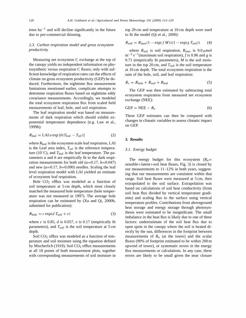
top 20 cm and temperature at 10 cm depth were usedto fit the model (Qi et al., 2000):

Rsoil = Rmax(1 − exp(f M))(1 − exp(g Tsoil)) (4)

where Rsoil is soil respiration,Rmax is 9.0mmolm−2 s−1(maximum soil respiration),f is 0.96 andg is0.71 (empirically fit parameters),M is the soil mois-ture in the top 20 cm, andTsoil is the soil temperatureat 10 cm depth. The total ecosystem respiration is thesum of the bole, soil, and leaf respiration:

Re = Rbole + Rsoil + Rleaf (5)

The GEP was then estimated by subtracting totalecosystem respiration from measured net ecosystemexchange (NEE):

GEP= NEE− Re (6)

These GEP estimates can then be compared withchanges in climatic variables to assess climatic impacton GEP.

3. Results

3.1. Energy budget

The energy budget for this ecosystem (Rn=sensible+latent+soil heat fluxes, Fig. 3) is closed byour measurements to 11–12% in both years, suggest-ing that our measurements are consistent within thatrange. Soil heat fluxes were measured at 5 cm, thenextrapolated to the soil surface. Extrapolation wasbased on calculations of soil heat conductivity (fromsoil heat flux divided by vertical temperature gradi-ents) and scaling flux to the surface using verticaltemperature profiles. Contributions from abovegroundheat storage and energy storage through photosyn-thesis were estimated to be insignificant. The smallimbalance in the heat flux is likely due to one of threefactors: underestimate of the soil heat flux due toopen spots in the canopy where the soil is heated di-rectly by the sun, differences in the footprint betweenmeasurements ofRn (at the tower) and the scalarfluxes (90% of footprint estimated to be within 200 mupwind of tower), or systematic errors in the energyflux measurements or calculations. In any case, theseerrors are likely to be small given the near closure


Fig. 3. Energy balance measurements of net radiation vs the sumof latent, sensible, and soil heat fluxes for the entire 1997 and1998 measurement periods. The solid line represents the ideal casewith a slope equal to 1.0; the dashed line indicates the best fit,which has slope of approximately 0.9 for both years.

of the energy budget and will not affect any of theconclusions drawn in this paper.

3.2. Time period averages

The impact of the interannual differences in climateon CO2, H2O, and sensible heat fluxes can be assessedthrough changes in their midday mean values over thegrowing season and in their mean diurnal cycles forboth years. To compare diurnal cycles of fluxes underdifferent conditions, four time periods were chosen todivide the growing season into differing soil moistureand VPD regimes. These time periods are 25 days longand begin on Day 153 of each year.

In 1997, the first period (Days 153–178) representsthe period of highest soil moisture and lowest VPD;the second period (Days 178–203) was a period of de-creasing soil moisture and moderate VPD; the thirdperiod (Days 203–228) was similar, except it includeda short event of extremely high VPD; and the fourth

period (Days 228–253) was a period of low soil mois-ture with a minor rain event, and moderate to lowVPD. These trends are similar in the 1998 data, exceptthat soil moisture was higher, needle development oc-curred later, and high VPD events were more frequent.

3.3. Environmental variables

Values for the environmental variables that moststrongly influence CO2 and energy fluxes are shownin Fig. 4 as time series for 1997 and 1998. These vari-ables are soil moisture, PAR, air temperature, and day-time mean (09:00–15:00 h PST) VPD. Vertical linesin these figures indicate the starting and ending pointsfor the four averaging periods defined in Section 3.2.Soil moisture (Fig. 4a) decreased over both seasons,although it was much higher throughout the 1998 mea-surement period. Photosynthetically active radiation(Fig. 4b) was similar for both years, remaining approx-imately constant over the comparison periods withslight variations due to cloud cover and the expectedseasonal progression of sun angle and day length. Airtemperature (Fig. 4c) varied, with coldest tempera-tures in the first period and extreme warm temperatureevents in the third period in 1997 and in the third andfourth periods in 1998. Additionally, the first periodwas significantly colder in 1998, delaying bud breakand needle elongation. The short-term (2–5 days) os-cillations in air temperature were associated with pass-ing weather fronts. VPD (Fig. 4d) varied with seasonand passing weather fronts in a manner similar to airtemperature.

3.4. Ecosystem response to environmental variables

Fluxes of sensible heat, H2O, and CO2 are presentedas mean diurnal cycles during the four averagingperiods (Fig. 5).

3.4.1. Heat fluxThe seasonal pattern in sensible heat fluxFsh

(Fig. 5a) varied between 1997 and 1998. In 1997,Fshwas consistent during the first and second averagingperiods. During the third and fourth periods (in-cluding the high temperature event and afterwards),sensible heat flux increased by roughly 30%, with aslight shift of the maximum flux earlier in the day.


Fig. 4. Time series of environmental variables that most strongly influence CO2 and energy fluxes including (a) soil moisture, (b) dailymaximum photosynthetically active radiation measured at the top of the tower, (c) air temperature measured at the top of the tower, and(d) vapor pressure deficit presented as midday (09:00–15:00 h PST) mean values. Vertical lines separate the averaging periods presentedin Figs. 5 and 8.

In 1998,Fsh decreased steadily from its peak valuesduring the first period, reaching a minimum in Period3 and then increasing somewhat during Period 4.

3.4.2. H2O fluxMean daytime H2O flux (Fig. 5b) was not statis-

tically different over the first three periods in 1997.During the heat spell of the third period, the waterflux increased rapidly to extremely high values in themorning, decreased until 12:00 h then remained rela-tively steady until sunset (data not shown separately).During this period of high temperatures, VPD rose toits highest observed values and early afternoon H2Ofluxes were depressed by approximately 25% com-

pared to the previous periods. The diurnal cycle of thisperiod was distinct from the rest of the summer. Afterthis event (Period 4), H2O flux was significantly lowerfor the remainder of the 1997 measurement period. Incontrast, H2O fluxes in 1998 followed a more sym-metrical pattern of starting out low, becoming higherduring midseason, and then decreasing again duringlate season; in 1998 they did not show sensitivity tosimilarly high VPD and temperature events.

3.4.3. Bowen ratioAfter the high temperature event in 1997 (Period

3), the maximum ecosystem Bowen ratio increasedabruptly from less than 1 to greater than 1 (Fig. 6).


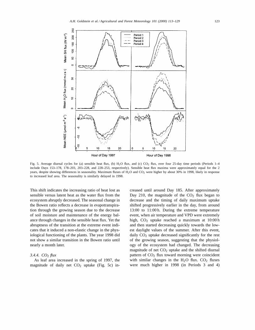
Fig. 5. Average diurnal cycles for (a) sensible heat flux, (b) H2O flux, and (c) CO2 flux, over four 25-day time periods (Periods 1–4include Days 153–178, 178–203, 203–228, and 228–253, respectively). Sensible heat flux maxima were approximately equal for the 2years, despite showing differences in seasonality. Maximum fluxes of H2O and CO2 were higher by about 30% in 1998, likely in responseto increased leaf area. The seasonality is similarly delayed in 1998.

This shift indicates the increasing ratio of heat lost assensible versus latent heat as the water flux from theecosystem abruptly decreased. The seasonal change inthe Bowen ratio reflects a decrease in evapotranspira-tion through the growing season due to the decreaseof soil moisture and maintenance of the energy bal-ance through changes in the sensible heat flux. Yet theabruptness of the transition at the extreme event indi-cates that it induced a non-elastic change in the phys-iological functioning of the plants. The year 1998 didnot show a similar transition in the Bowen ratio untilnearly a month later.

3.4.4. CO2 fluxAs leaf area increased in the spring of 1997, the

magnitude of daily net CO2 uptake (Fig. 5c) in-

creased until around Day 185. After approximatelyDay 210, the magnitude of the CO2 flux began todecrease and the timing of daily maximum uptakeshifted progressively earlier in the day, from around13:00 to 11:00 h. During the extreme temperatureevent, when air temperature and VPD were extremelyhigh, CO2 uptake reached a maximum at 10:00 hand then started decreasing quickly towards the low-est daylight values of the summer. After this event,daily CO2 uptake decreased significantly for the restof the growing season, suggesting that the physiol-ogy of the ecosystem had changed. The decreasingmagnitude of net CO2 uptake and the shifted diurnalpattern of CO2 flux toward morning were coincidentwith similar changes in the H2O flux. CO2 fluxeswere much higher in 1998 (in Periods 3 and 4)


Fig. 6. Bowen ratio (sensible/latent heat fluxes) presented as midday mean values (09:00–15:00 h PST) over the whole measurement period,showing a steady decrease as the ecosystem became drier over the course of the summer. Values were excluded for standard errors greaterthan 1.

but also exhibited earlier maxima for Periods 1, 2,and 4.

3.4.5. Gross ecosystem productivityMeasured NEE, modeled ecosystem respirationRe,

and resultant ecosystem productivity GEP for bothyears are presented in Fig. 7 as midday mean val-ues. Years 1997 and 1998 had noticeably differentCO2 exchange characteristics. The modeled daytimemean ecosystem respiration was approximately 25%higher during 1998, primarily as a result of wetterconditions increasing the soil respiration componentand the increase of respiring leaf and bole area dueto tree growth. The maximum measured NEE wasalso slightly larger in 1998. The differences betweenthe years are most pronounced for GEP. The primary

difference in the GEP pattern lies in the timing of themaximum value: in 1997, maximum GEP occurredaround Days 190–220, while 1998 had its maximanearly a month later (Days 210–240). Furthermore,whereas the 1998 GEP exhibited a gradual decreasefrom peak values, the 1997 GEP values exhibit amuch sharper decrease following their peak values.Maximum daytime mean GEP was approximately25% greater in 1998 (with a change from−20 to−25mmol m−2 s−1), a difference that is consistentwith the 30–35% increase in maximum LAI over 1997.

4. Discussion

The close correlation of the high temperature/VPDevent in 1997 and the step change in Bowen ratio and


Fig. 7. Daytime mean measured NEE (circles) plotted with modeled respiration (triangles) and resultant GEP (squares) for 1997 and 1998.Note the difference in timing of maximum GEP, with 1998 peaking much later due to delayed leaf development. Note also the 1997change in GEP from−19 to −15mmol m−2 s−1 after the extreme VPD event at Day 220.

carbon sequestration suggests that the productivity ofthe study ecosystem can undergo sharp changes in re-sponse to extreme weather events. Furthermore, thepresence of equally high extreme temperature/VPDevents in 1998 without associated abrupt changes inwater and carbon fluxes indicates that the sensitivityof the system also depends on other climatic factors.These factors, which may involve longer-timescaleevents like the timing of snowmelt or the frequencyand distribution of rainfall events, also influence thetiming of phenological changes in spring and there-fore the length of time during which the plants canphotosynthesize.

Seasonal variations in leaf area, incident sunlight,temperature, VPD, and soil moisture are expected toexert control on the net transfer of CO2, H2O, andsensible heat between vegetation and the atmospherebecause these variables control photosynthesis, res-piration, and transpiration. Leaf area determines the

amount of available photosynthetic and transpiringmaterial and the amount of light intercepted by the for-est. Temperature affects rates of enzyme kinetics as-sociated with photosynthesis and respiration, and soilmoisture and VPD affect the hydraulic status of plantsand leaves, and therefore stomatal conductance.

In 1997, leaf area increased during the first aver-aging period then remained fairly constant over thelast three; thus, the initial increase in net CO2 uptakecould be attributed to increasing leaf area, but this pa-rameter would seem not to exert a strong influence onC fluxes after this time. However, as noted earlier, thetiming of leaf elongation was offset by approximately1 month in 1998, and this delay was also reflected ina delay in the timing of maximum NEE. As Fig. 5indicates, NEE peaked in Period 2 in 1997 but not un-til Periods 3 and 4 in 1998. The amount of availablePAR establishes an upper limit for canopy photosyn-thesis, so the gradual decrease (by about 15%) of day-


time maximum PAR over the four periods likely ledto a small decrease of net CO2 uptake but had sim-ilar timing for both years. The remaining parameters(air temperature, VPD, and soil moisture content) var-ied more markedly over the measurement periods andthus likely influenced the different patterns of fluxesobserved in the 2 years.

The magnitudes of observed NEE and GEP in thisecosystem reflect the rapid growth rates characteristicof a young, even-aged forest. Anthoni et al. (1999) re-port significantly lower maximum daytime NEE val-ues for an older drought-stressed ponderosa pine forestin Oregon with total LAI of 3.2 (∼7mmol m−2 s−1,compared with∼15mmol m−2 s−1 for this site in1997). A more thorough comparison of these twoecosytems is presented in Law et al. (2000b, submit-ted for publication).

4.1. Controls on H2O flux

Stomata provide the primary pathways for plantH2O loss. Increasing VPD can cause the H2O flux toincrease if the stomatal conductance remains constant,but could also cause a reduction in stomatal conduc-tance, thus reducing H2O flux. Fig. 8 compares meanmidday H2O flux with VPD for the different periods:before (Periods 1 and 2), during (Period 3), and af-ter (Period 4) the extreme temperature event in 1997.Note that the mean midday H2O flux was significantlyreduced (by over 30%) after this event. The changein relationship between H2O flux and VPD after theextreme temperature event could be due to crossinga critical threshold of soil moisture (approximately10% at 20 cm on Day 221), but this seems unlikelygiven that the soil moisture was steadily decreasing by0.04% per day during this period. Thus, the shift in re-lationship between H2O flux and VPD is more likelydue to a physiological change in the plants during theevent that persisted for the remainder of the growingseason.

One possible change is cavitation in the water con-ducting system of the plants. Because trees and otherplants maximize their carbon uptake per unit waterlost, stomata may remain open until tension in thexylem reaches a critical threshold just prior to catas-trophic cavitation. Thus, trees function very near thecavitation point (Tyree and Sperry, 1988). While it is

Fig. 8. Relationship between vapor pressure deficit and H2Oflux (Periods 1–4 include Days 153–178, 178–203, 203–228, and228–253, respectively). After the extreme event in 1997 (whichcan be seen in the two outlier points for Period 3), H2O fluxesdecreased significantly. No similar patterns were seen in 1998 asa result of similar extreme events in Period 3, although there issome evidence that the two extreme VPD events in Period 4 mayhave begun a similar shift.

deleterious for trees to cavitate during the growingseason because they lose important water conductingvessels, it is not unusual to observe the phenomenon(Zimmermann, 1963; Tyree and Sperry, 1989). There-fore, the unusually high H2O flux early in the morningduring the extreme event could result from extra wa-ter release from cavitating tracheids. After this event,mean conductance was lower than pre-heat spell lev-els, a state consistent with the loss of conducting areain the xylem of the plants (Tyree and Ewers, 1991;Panek and Waring, 1995).

No similar event-driven changes in the relationshipbetween VPD and H2O flux were observed in 1998(Fig. 8). Although higher VPD events did occur in1998, the soil moisture was also higher than in 1997,suggesting the ecosystem is sensitive to extreme heatevents only when soil moisture is low.


4.2. Controls on the Bowen ratio

Because the Bowen ratio reflects the ecosystem’spartitioning of incoming energy between water flux(largely dominated by plant transpiration during thesummer) and sensible heat flux (that does not directlyreflect plant physiology), it provides a good indicatorof the relative physiological activity of the ecosystem.Thus, Fig. 6 demonstrates not only the abruptness inecosystem change after the 1997 extreme event butalso provides a rough indication of the timing of sea-sonal ecosystem shifts. That the ecosystem in 1998 ex-perienced a similar low Bowen-ratio regime for nearly40 days after the time of the extreme 1997 event sug-gests that the ecosystem does not have an inherentphysiological limitation that begins at Day 220 butrather responds to extant environmental conditions.

4.3. Controls on CO2 flux and GEP

Major ecosystem C fluxes (NEE,R, GEP) for bothmeasurement seasons are presented in Fig. 7. The ex-

Fig. 9. Cumulative NEE for 1997 and 1998. Gaps in the data were filled by modeling NEE as a function ofT, PAR, andM based onavailable data. If these data were missing, gaps were filled by interpolating the average diurnal cycles from 3 days before and after themissing time period. Nighttime data were replaced using the respiration model whenu*<0.17 and when the wind was not coming fromthe main tower fetch direction.

treme event of 1997, which considerably influencedthe water vapor flux, had a similar effect on GEP(and thus NEE). Less than a week after the event,daytime mean GEP had decreased by approximately20%. Since 1998 did not show a similar decrease inGEP during the same period (despite several high VPDevents), the low soil moisture seems to have combinedwith the extreme VPD event in 1997 to produce thisstep change in ecosystem C cycling rate. This result isconsistent with the hypothesis that the ecosystem ex-perienced a step change in the ability ofP. ponderosato photosynthesize as the result of an extremely hightemperature and VPD event at Day 220. A similar de-crease was not observed in 1998 until nearly 30 dayslater, indicating that the extreme event initiated anearly decrease in the ecosystem’s carbon sequestrationpotential in 1997. In cumulative terms, this reductionof 20% of GEP over 30 days results in a decreasedsequestration of over 90 g C m−2 land area. If we as-sume that the seasonality in productivity changes in1998 represents an ideal maximum, this decreased se-questration accounts for a roughly 5–10% reductionin the total 1997 growing season sequestration.


Cumulative NEE curves (Fig. 9) also provide anoverview of differences in carbon uptake between1997 and 1998. The earlier onset of photosynthesis isevident as the 1997 curve shows higher cumulativesequestration (relative to Day 153) in the first half ofthe growing season. Later, the larger 1998 LAI anddecreased 1997 uptake due to the extreme event ledto the much larger ultimate 1998 sequestration. ByDay 200, 1997 cumulative NEE was 19% higher thanin 1998, but by Day 253, this balance shifted suchthat the 1998 cumulative NEE for Days 153–253 was18% higher than in 1997.

5. Conclusions

The ponderosa pine ecosystems of the western USfunction differently from many other ecosystems mon-itored by eddy correlation due to the annual sum-mertime drought stress. The ponderosa pines are welladapted to this climate, but our results suggest thattheir carbon uptake rates will respond in unique andimportant ways to changes in climate and hydrologicregime.

Our data set provides distinct periods under whichthe separate influences of environmental variables canbe observed. By investigating the effects of differentcombinations of variables during different periods, wewere able to determine that the system exhibits somemodes that are prone to change abruptly after an ex-treme climatic perturbation. Specifically, we observedthat the relationship between soil moisture, VPD, andconductance is complex and can respond nonlinearlyto an extreme VPD event when the soil moisture isalready low. Correctly modeling the changes in phys-iological activity after extreme drought stress eventsrequires appropriate representation of event-drivenphysiological changes (such as cavitation) in theecosystem’s capacity for photosynthesis and respi-ration, in addition to their direct response to soilmoisture and VPD.

Based on our measurements, the major factors thataffected carbon uptake in this ecosystem were (a) thetiming of new leaf development, (b) the severity ofseasonal drought conditions (soil moisture), and (c)the timing and severity of extreme events with highVPD which can affect the physiological function ofthe ecosystem for the remainder of the growing sea-

son. Variability in climate and hydrology should havesignificant impacts on carbon uptake and physiolog-ical function of Mediterranean-type drought-stressedecosystems. If an extremely high VPD event occursearly in the season in a dry year, and causes physiolog-ical damage to the plants, annual carbon uptake ratescould be severely reduced. If no high VPD events oc-cur and/or soil moisture is higher, annual carbon up-take rates could be significantly enhanced. Therefore,climate change in this type of ecosystem can causelarge interannual variability in carbon storage.

Acknowledgements

This research was supported by the EnvironmentalProtection Agency (Award Number R826601), theUniversity of California at Berkeley, the Universityof California Agricultural Experiment Station, theNational Center for Atmospheric Research (Boul-der, CO), the William and Flora Hewlett Foundation,the Swiss National Fund, and the Blodgett ForestResearch Station. The authors thank Sierra PacificIndustries for permission to carry out this research ontheir property and Scott Chambers for help with dataanalysis. We also thank Mark Lamanna, Bob Heald,Dave Rambeau, Frieder Schurr, and the BlodgettForest crew for their invaluable support during fieldoperations.

References

Anthoni, P.M., Law, B.E., Unsworth, M.H., 1999. Carbon andwater vapor exchange of an open-canopied ponderosa pineecosystem. Agric. For. Meteorol. 95, 151–168.

Baker, B., Guenther, A., Greenberg, J., Goldstein, A., Fall, R.,1999. Canopy fluxes of 2-methyl-3-buten-2-ol over a ponderosapine forest: field data and model comparison. J. Geophys. Res.104, 26107–26114.

Baldocchi, D., Hicks, B., Meyers, T., 1988. Measuringbiosphere–atmosphere exchanges of biologically related gaseswith micrometeorological methods. Ecology 69, 1331.

Baldocchi, D., 1997. Measuring and modelling carbon dioxide andwater vapour exchange over a temperate broad-leaved forestduring the 1995 summer drought. Plant, Cell and Environ. 20,1108.

Baldocchi, D.D., Law, B.E., Anthoni, P.M., 2000. On measuringand modeling energy fluxes above the floor of a homogeneousand heterogeneous conifer forest. Agric. For. Meteorol., in press.


Chambers, S.D., Hacker, J.M., Williams, A.G., 1997. RAMFVersion 8.1 User’s Manual, 2nd Edition. FIAMS TechnicalReport 14, 150 pp.

Chen, J.M., Cihlar, 1996. Optically-based methods for measuringseasonal variation of leaf area index in boreal conifer stands.Agric. For. Meteorol. 80, 135–163.

Clark, K.L., Gholz, H.L., Moncrieff, J.B., Cropley, F., Loescher,H.W., 1999. Environmental controls over net exchanges ofcarbon dioxide from contrasting Florida ecosystems. Ecol.Applications 9 (3), 936–948.

Goulden, M.L., Munger, J.W., Fan, S.M., Daube, B.C., Wofsy,S.C., 1996. Measurements of carbon sequestration by long-termeddy covariance: methods and a critical evaluation of accuracy.Global Change Biol. 2, 169.

Grace, J., Lloyd, J., McIntyre, J., Miranda, A., Meir, P., Miranda,H., Moncrieff, J.B., Massheder, J.M., Wright, I., Gash, J., 1995.Fluxes of carbon dioxide and water vapor over an undisturbedtropical forest in South-West Amazonia. Global Change Biol.1, 1.

Horst, T.W., Weil, J.C., 1994. How far is far enough? The fetchrequirements for micrometeorological measurement of surfacefluxes. J. Atmos. Oceanic Technol. 11, 1018–1025.

Hsieh, C.I., Katul, G.G., Schieldge, J., Sigmon, J.T., Knoerr, K.R.,1997. The Lagrangian stochastic model for fetch and latent heatflux estimation above uniform and non-uniform terrain. WaterResources Res. 33, 427–438.

Lamanna, M.S., Goldstein, A.H., 1999. In-situ measurements ofC2-C10 VOCs above a Sierra Nevada ponderosa pine plantation.J. Geophys. Res. 104, 21247–21262.

Landram, M., 1996. Sierra Nevada Ecosystem Project Final Reportto Congress, III. Wildland Resources Center Report No. 38,University of California, Davis, pp. 513–542.

Law, B.E., Ryan, M.G., Anthoni, P.M., 1999a. Seasonal and annualrespiration of a ponderosa pine ecosystem. Global Change Biol.5, 169–182.

Law, B.E., Baldocchi, D.D., Anthoni, P.M., 1999b. Below-canopyand soil CO2 fluxes in a ponderosa pine forest. Agric. For.Meteorol. 94, 13–30.

Law, B.E., Waring, R.H., Anthoni, P.M., Aber, J.D., 2000a.Measurements of gross and net ecosystem productivity andwater vapor exchange of aPinus ponderosaecosystem, andan evaluation of two generalized models, and an evaluationof two generalized models. Global Change Biol. 6, 155–168.

Law, B.E., Goldstein, A.H., Anthoni, P.M., Unsworth, M.H., Panek,J.A., Bauer, M.R., Fracheboud, J.M., Hultman, N., 2000b. CO2

and water vapor exchange by young and old ponderosa pineecosystems during a drought year. Tree Physiol., submitted forpublication.

Leuning, R., King, K.M., 1992. Comparison of eddy-covariancemeasurements of CO2 fluxes by open-path and closed-path CO2

analysers. Boundary-Layer Meteorol. 59 (3), 297–311.

Margolis, H.A., Ryan, M.G., 1997. A physiological basis forbiosphere-atmosphere interactions in the boreal forest: anoverview. Tree Physiol. 17, 8–9.

Mischerlich, J.L., 1919. The law of plant growth. In: Lieth,H.F. (Ed.), Patterns of Primary Productivity in the Biosphere.Benchmark Papers in Ecology, 8. Dowden, Hutchinson andRoss, Inc., Strausbourg, Penn, 1978, 239 pp.

Moncrieff, J.B., Malhi, Y., Leuning, R., 1996. The propagation oferrors in long-term measurements of land-atmosphere fluxes ofcarbon and water. Global Change Biol. 2, 231.

Musselman, R.C., Fox, D.G., 1991. A review of the role oftemperate forests in the global CO2 balance. J. Air WasteManage. Assoc. 41, 798.

Panek, J.A., Waring, R.H., 1995. Carbon-isotope variation inDouglas-fir foliage: improving thed13C-climate relationship.Tree Physiol. 15, 657–663.

Qi, Y., Xu, M., Goldstein, A.H., 2000. Modeling jointeffect of temperature and moisture on soil CO2 efflux: anon-Q10 approach. American Geophysical Union Fall Meeting,supplement to EOS, Transactions, Vol. 80, H52A–12.

Rissmann, J., Tetzlaff, G., 1994. Application of a spectralcorrection method for measurements of covariances withfast-response sensors in the atmospheric boundary layer up to aheight of 130 m and testing of the corrections. Boundary-LayerMeteorol. 70 (3), 293–305.

Shuttleworth, W.J., Gash, J.H., Lloyd, C.R., Moore, C.J.,Roberts, J., Filho, A.O.M., Fisch, G., Filho, V.P.S., Ribeiro,M.N.G., Molion, L.C.B., Sa, L.D.A., Nobre, J.C.A., Cabral,O.M.R., Patel, S.R., De Moraes, J.C., 1984. Eddy CorrelationMeasurements of Energy Partition for Amazonian Forest. Q. J.R. Meteorol. Soc. 110, 1143–1162.

Tyree, M.T., Ewers, F.W., 1991. The hydraulic architecture of treesand other woody plants (Tansley Review No. 34). New Phytol.119, 345–360.

Tyree, M.T., Sperry, J.S., 1989. Vulnerability of xylem to cavitationand embolism. Annu. Rev. Plant Physiol. Mol. Biol. 40, 19–38.

Tyree, M.T., Sperry, J.S., 1988. Do woody plants operate nearthe point of catastrophic xylem dysfunction caused by dynamicwater stress? Answers from a model. Plant Physiol. 88, 574–580.

Wofsy, S.C., Goulden, M.L., Munger, J.W., Fan, S.M., Bakwin,P.S., Daube, B.C., Bassow, S.L., Bazzaz, F.A., 1993. Netexchange of CO2 in a mid-latitude forest. Science 260 (5112),1314–1317.

Xu, M., DeBiase, T.A., Qi, Y.A., 2000a. A simple techniqueto measure stem respiration using horizontally-oriented soilchamber. C. J. For. Res., submitted for publication.

Xu, M., Qi, Y., 2000b. Stem respiration in a young ponderosa pineplantation in Sierra Nevada Mountains, California. For. Ecol.Manage., submitted for publication.

Zimmermann, M.H., 1963. How sap moves in trees. Sci. Am. 154,3–10.

effects of climate variability on the carbon dioxide, water, and

Documents