effects of agricultural commercialization on land tenure...

RESEARCH REPORT

EFFECTS OF AGRICULTURALCOMMERCIALIZATION ONLAND TENURE, HOUSEHOLDRESOURCE ALLOCATION,AND NUTRITION IN THEPHILIPPINESHowarth E. BouisLawrence J. Haddad

January 1990

INTERNATIONALFOODPOLICYRESEARCHINSTITUTE

In collaboration with the

RESEARCHINSTITUTEFOR MINDANAOCULTURE

The International Food Policy ResearchInstitute was established in 1975 to identifyand analyze alternative national and inter-national strategies and policies for meetingfood needs in the world, with particular em-phasis on low-income countries and on thepoorer groups in those countries. While theresearch effort is geared to the precise ob-jective of contributing to the reduction ofhunger and malnutrition, the factors involvedare many and wide-ranging, requiring analy-sis of underlying processes and extendingbeyond a narrowly defined food sector. TheInstitute's research program reflects world-wide interaction with policymakers, adminis-trators, and others concerned with increasingfood production and with improving theequity of its distribution. Research resultsare published and distributed to officials andothers concerned with national and inter-national food and agricultural policy.

The Institute receives support as a consti-tuent of the Consultative Group on Interna-tional Agricultural Research from a numberof donors including Australia, Belgium,Canada, the People's Republic of China, theFord Foundation, France, the Federal Re-public of Germany, India, Italy, Japan, theNetherlands, Norway, the Philippines, theRockefeller Foundation, Switzerland, theUnited Kingdom, the United States, and theWorld Bank. In addition, a number of othergovernments and institutions contributefunding to special research projects.

Board of Trustees

Dick de ZeeuwChairman, Netherlands

Harris Mutio MuleVice Chairman, Kenya

Sjarifuddin BaharsjahIndonesia

Yahia BakourSyria

Claude CheyssonFrance

Anna Ferro-LuzziItaly

Yujiro HayamiJapan

Gerald Karl HelleinerCanada

Roberto JunguitoColombia

Dharma KumarIndia

James R. McWilliamAustralia

Theodore W. SchultzU.S.A.

Leopoldo SolisMexico

M. SyeduzzamanBangladesh

Charles Valy TuhoC6te d'lvoire

John W. Mellor, DirectorEx Officio, U.S.A.

EFFECTS OF AGRICULTURALCOMMERCIALIZATION ON LAND TENURE,HOUSEHOLD RESOURCE ALLOCATION,AND NUTRITION IN THE PHILIPPINES

Howarth £. BouisLawrence J. Haddad

Research Report 79International Food Policy Research Institutein collaboration with theResearch Institute for Mindanao CultureJanuary 1990

Copyright 1990 International Food PolicyResearch Institute.

All rights reserved. Sections of this report maybe reproduced without the express permission ofbut with acknowledgment to the InternationalFood Policy Research Institute.

Library of Congress Cataloging-in-Publication Data

Bouis, Howarth E.Effects of agricultural commercialization on

land tenure, household resource allocation, andnutrition in the Philippines/Howarth E. Bouis,Lawrence J. Haddad.

p. cm. — (Research report/InternationalFood Policy Research Institute ; 79)

"January 1990."Includes bibliographical references.ISBN 0-89629-081-61. Agriculture — Economic aspec ts —

Philippines. 2. Produce trade —Philippines.3. Land tenure—Philippines. 4. Households-Ph i l ipp ines . 5. Nutr i t ion —Phi l ippines .I. Haddad, Lawrence James. II. InternationalFood Policy Research Institute. III. Xavier Uni-versity (Cagayan de Oro City, Philippines).Research Institute for Mindanao Culture.IV. Title. V. Series: Research report (Interna-tional Food Policy Research Institute) ; 79.HD2087.B68 1990 89-71649338.1'09599-dc20 CIP

CONTENTS

Foreword

1. Summary 9

2. Research Objectives and PolicySetting 11

3. Conceptual Framework andResearch Design 15

4. Changes in Land TenurePatterns 22

5. Comparison of the Corn andSugar Production Systems 29

6. Food Expenditures and CalorieIntakes 40

7. Heights and Weights of Pre-school Children 48

8. Conclusions 56

Appendix 1: Should the Model BeTreated as Simul-taneous or Recursive? 60

Appendix 2: Total Expendituresand Household Calo-rie Availability asProxies for Incomeand Household Calo-rie Intakes 62

Appendix 3: Descriptive Statisticsand Results of F-Testsand Tests for Exog-eneity 66

Bibliography 70

TABLES

1. List of topics covered by surveyquestionnaires, 1984/85 19

2. Selected data for respondenthouseholds, by crop-tenancygroup, 1984/85 20

3. Percentage distribution ofsugar and corn farms and areaharvested in Bukidnon Pro-vince, by farm size, 1971 and1980 23

4. Present primary occupation ofheads of households, all munic-ipalities, April 1984 24

5. Sugar-producing households,by land tenure and previousoccupation, April 1984 25

6. Household employment andland tenure status duringround 4 of survey and beforesugar mill operation, July 1985 26

7. Comparison of past and presentcorn yields, by crop-tenancygroup and farm size, 1984/85 30

8. Total labor inputs per corncrop, by family and hired labor,crop-tenancy group, and farmsize, 1984/85 31

9. Shelled corn production andconsumption of own production,by crop-tenancy group and farmsize, 1984/85 32

10. Sugar yields, by crop-tenancygroup and milling season,1984/85 34

11. Total labor inputs per sugarcrop, by crop-tenancy groupand family and hired labor,1984/85 34

12. Corn and sugar productionprofits, by crop-tenancy groupand farm size, 1984/85

14. Sources of income, by expendi-ture quintile and crop-tenancygroup, 1984/85

36

13. Labor inputs for corn and sugar,by family and hired labor,1984/85 37

38

15. Income, expenditures, and calo-rie availability and intake, byincome and expenditure quin-tiles and crop-tenancy group,1984/85 41

16. Regression results for the rela-tionship between income andfood expenditures 42

17. Allocation of weekly per capitafood expenditures, by foodgroup, expenditure quintile,and crop-tenancy group,1984/85 43

18. Regression results for the rela-tionship between calorieintakes and food expenditures 44

19. Calorie adequacy, by familymember, expenditure quintile,and crop-tenancy group,1984/85 45

20. Regression results for pre-schooler calorie intakes as afunction of household calorieintakes 46

21. Z-scores for height-for-age,weight-for-age, and weight-for-height of preschoolers, by ageand expenditure quintile,1984/85 48

22. Height-for-age Z-scores for pre-schoolers who no longer breast-feed, by crop-tenancy group andage tercile, 1984/85 49

23. Mothers' time away from thehouse, by breastfeeding statusand crop-tenancy group,1984/85 51

24. Prevalence of sickness amongbreast feeding and non-breastfeeding preschoolers, byexpenditure quintile and crop-tenancy group, 1984/85 52

25. Regression results for the rela-tionship between preschoolers'calorie intake and weight-for-height 54

26. Income elasticities of house-hold calorie consumptionimplied by the two-way relation-ship between income andhousehold calorie intakes 64

27. Descriptive statistics for vari-ables used in regressionanalysis 66

28. Results of testing for equalityof coefficients between cornand sugar households 68

29. Results of Hausman tests forexogeneity of right-hand sidevariables 69

ILLUSTRATIONS1. Map of the Philippines indicating

study area 14

2. Household resource allocationand nutrition 16

FOREWORD

Over the past several years IFPRI has undertaken research on the production,consumption, and nutrition effects of agricultural commercialization in The Gambia,Guatemala, Kenya, the Philippines, and Rwanda. While it is widely recognized that thecommercialization of agriculture is essential to overall economic development, variousrural population groups adapt differently to the process of commercialization, depend-ing on the resources available to them, economic and social conditions, and governmentpolicies. Many households benefit in the form of higher incomes; others may suffer adecline in income. A particular concern of policymakers has been the effect ofcommercialization on nutrition.

The purpose of these studies has been to analyze the process of commercializationin order to identify key factors that determine nutritional outcomes, with the objective offormulating policies to enhance the beneficial effects of commercialization and minimizethe harmful effects.

The present report by Howarth E. Bouis and Lawrence J. Haddad presents thefindings for the Philippine case study, located in an area on the southern island ofMindanao where a substantial number of households converted lands from corn tosugarcane production after construction of a sugar mill. The main effects of theintroduction of export cropping in this area were a significant deterioration in access toland as smallholder corn tenant farms using primarily family labor were consolidatedinto larger sugar farms using primarily hired labor; an increase in incomes forhouseholds that grew sugarcane; a decline in women's participation in own-farmproduction; and very little improvement in nutritional status as a result of increasedincomes from sugarcane production, primarily because of the high levels of preschoolersickness in the sugarcane-growing households.

The difficulty of generalizing as to the varied effects of agricultural commercializa-tion is brought out by a comparison with the case study for Kenya (see IFPRI ResearchReport 63 by Eileen Kennedy and Bruce Cogill), where farmers also switched frommaize to sugarcane production. In that African setting, where land is often relativelyabundant and labor scarce compared with many situations in Asia, women increasedtheir participation in own-farm production as sugarcane was introduced. Yet there areimportant similarities as well. As all of the commercialization studies have confirmed,poor health and sanitation conditions are a serious constraint to the improved nutritionthat increases in income might otherwise have made possible.

John W Mellor

Washington, D.C.January 1990

ACKNOWLEDGMENTS

This report has been many years in the making, and we would like to acknowledgeseveral people who gave more of themselves than we could have reasonably expectedand without whom the report would not have been possible.

We thank all the staff at the Research Institute for Mindanao Culture, especially thesupervisors under the direction of Lourdes Wong. The project was literally in theirhands for a year and a half and we learned a lot from them about how a survey should berun. We are indebted to Father Francis Madigan for putting together such a professionalstaff over so many years of dedicated work at RIMCU.

We are deeply grateful to Azucena Limbo of the Nutrition Foundation of thePhilippines, who provided training for collection of our anthropometric and 24-hourfood-recall data, no doubt the most difficult portion of our questionnaire to administerand code. Her competence and enthusiasm helped us through some difficult times.

We thank Joel Asentista, head of the Xavier University extension program inBukidnon, and Roberto Montalvan, president of the Bukidnon planters association, forgiving up so much of their personal time to familiarize us with the study area, as well asFather Antonio Ledesma and the graduate students of the Institute for Market Analysisat Xavier University, whose background knowledge of the area and logistical supportwere essential inputs into our survey work.

The help of Per Pinstrup-Andersen, whose efforts provided the initial impetus formany of the IFPRI commercialization studies, is gratefully acknowledged. For detailedcomments on various drafts of the entire report, we would like to thank Romeo Bautista,Rodolfo Florentine Yujiro Hayami, Francis Madigan, John Mellor, and Steve Vosti. Forhelpful comments on specific components of the study, we would like to thank JulieAnderson, Gelia Castillo, Reynaldo Martorell, Marc Nerlove, and Anne Peck. Any errorsand omissions remaining in the report are, of course, our responsibility alone.

Finally, we thank the U.S. Agency for International Development for giving us theopportunity and freedom to undertake the research by funding the project (under GrantNo. OTR-OOOO-G-55-3513-00).

Howarth E. BouisLawrence J. Haddad

SUMMARYThe commercialization of agriculture, and in particular export cropping, has often

been blamed as a cause of poor nutrition. Critics contend that if the resources used toproduce agricultural exports were used instead to produce food for the local economy,the problem of malnutrition in many countries could be significantly reduced, or eveneliminated. Proponents argue that by exploiting comparative advantage and generatingfaster growth for the overall economy, export cropping raises incomes and improvesnutrition. In order to identify policy measures that can enhance positive and minimizeharmful nutrition effects, IFPRI has undertaken research on the process of agriculturalcommercialization in five specific country contexts. This research report presents thefindings for the Philippine case study.

Approximately 500 corn- and sugar-producing households were surveyed four timesat four-month intervals during 1984 and 1985 in one province in Mindanao, Bukidnon,an area primarily engaged in semisubsistence corn production before the establishmentof a sugar mill in 1977. The sample included smallholder landowner, tenant, andlandless laborer households. Data were collected on landholdings, income sources,expenditure patterns, calorie intakes, and nutritional status.

An initial random sample of households, both far away from the sugar mill(households that did not have the opportunity of switching to sugar because of the highcost of transporting cane to the mill) and near to the mill, indicated a seriousdeterioration in land tenancy patterns as a result of the introduction of sugar. Whereaslandless households accounted for less than 5 percent of households engaged primarilyin corn production, nearly 50 percent of households employed in sugar production hadno access to land. When households engaged in sugar production were asked tocharacterize their tenancy status before the introduction of sugar seven years earlier,the pattern of distribution that emerged between owner, share tenant, and landlesslaborer households was very similar to the present pattern for corn households. Severalformer corn tenant households had lost access to land when landlords who had decidedto grow sugarcane chose to hire labor for the new crop rather than rent out land on ashare-of-harvest basis, as had been the custom with corn.

The detailed survey data show that smallholder sugar landowners and renters whokept their land made substantially higher profits per hectare than their corn-householdcounterparts (an average of US$225 per hectare per year for sugar compared withUS$100 for corn) despite the low prevailing world prices for sugar, which to some extentwere transmitted to the domestic market. The higher profits for sugar are in part areflection of the low and declining productivity of corn. The primarily migrant popula-tion reported that corn yields, because of declining soil fertility, were about half of whatthey had been when they first settled their land. Despite this, all sugar households withaccess to land continued to plant some land to corn and, on average, produced well inexcess of their household needs.

On average, about two-thirds of the labor devoted to corn production is provided bythe family and one-third is hired. These fractions between family and hired labor arereversed for sugar production. Women contributed 23 percent of the total labor for cornproduction, but only 11 percent of the total labor for sugar production.

Sugar households had higher incomes on average than com households, due partlyto higher profits from sugar and partly to larger landholdings, although for mosthouseholds, sources of incomes were highly diversified, with 29 percent of all incomescoming from nonagricultural sources. The income elasticity for food expenditures at themean for all sample households was estimated to be 0.65, so that food expendituresrose rapidly with income. However, because higher-priced calories were purchased byhigher-income households, a doubling of income at mean income levels leads to only an11 percent increase in calorie intakes at the household level. A substantial portion of theextra calories that were available at higher incomes went to adults, who were alreadymeeting their recommended intakes of calories. Preschool children (once breastfeedinghad been stopped) at all income levels consumed well below their recommended calorieintakes.

A strong association exists between income and height-for-age, a long-run measureof nutritional status, for children less than one year old. However, this associationbetween income and height-for-age is weak for preschoolers at four years of age, whichmeans that height-for-age deteriorates (relative to average heights for a reference, well-nourished population) much faster for higher-income children than lower-income child-ren as they grow older. This aggregate pattern is more pronounced for the higher-incomesugar households. Preschool children who are four years of age from householdswithout access to land (corn and sugar landless laborer households) are significantlymore stunted than children of the same age in households with access to land, reflectingin part the low availability of calories in these landless households, which spend morethan three-fourths of their income on food.

Regressions show morbidity to be an important determinant of short-run nutritionalstatus, weight-for-height. There appears to be little association between income andmorbidity, although sugar-household children are sick more often than corn-householdchildren, which is consistent with the more rapid deterioration in height-for-age forsugar-household children as they grow older.

Export cropping can significantly raise the incomes of smallholder producers.However, to prevent further consolidation of smallholder farms, the government needsfirst to make a conscious effort to encourage export cropping by smallholders byproviding them with credit and know-how through extension and by actively promotingtheir access to processing and marketing facilities where necessary. Second, small-holder corn productivity needs to be improved. Both open-pollinated and hybrid varietiesare available, but typically only larger landowners in Bukidnon are experimenting withthe new corn technologies.

In the area of nutrition policy, providing landless households with access to landappears to be a sufficient condition for limited improvement in preschooler nutritionalstatus. However, for households with access to land, preschooler nutrition does notseem to improve as income increases. Regressions show calorie intakes of preschoolersto be positively and significantly related to their nutritional status. Yet higher-incomehouseholds choose to purchase nonfood items and higher-priced calories at the margin,while preschoolers continue to consume well below recommended intakes. Surelyeducation has some role to play in convincing parents to adjust food-expenditurebehavior and to distribute calories more equitably among household members. Eventhis, however, may not be sufficient given the high prevalence of preschooler sickness,even among high-income groups. Reducing illness may involve both education andimprovement of community-level health and sanitary conditions.

10

RESEARCH OBJECTIVES AND POLICY SETTING

Specialization, development of markets, and trade, which characterize com-mercialization, are fundamental to economic growth. But how are higher averageincomes distributed among various economic and social groups as commercializationtakes place? Does a higher household income necessarily mean better nutrition for allhousehold members? Because there are so many possible policy variations within thecompeting paradigms of specialization and self-sufficiency, because economic and socialconditions vary so much across countries and regions, and finally because there areinevitably winners and losers in any process of change, it is unfortunately impossible toanswer such crucial questions in any definitive way.

In order to provide some guidance for policy formulation in this area, however, whatis possible is to study the process of commercialization in specific contexts and toidentify key factors that appear to lead either to beneficial or detrimental outcomes interms of nutrition. In designing and carrying out future projects and policies, then, theresearch goal would be for policymakers to find ways to enhance the beneficial factors,while minimizing the harmful ones.

Toward this end, the International Food Policy Research Institute (IFPRI) hasconducted microlevel studies in five countries—The Gambia, Guatemala, Kenya, thePhilippines, and Rwanda—in rural areas where farm households have recently under-gone a switch from semisubsistence staple food production to production of cropsprimarily for sale in the market (Kennedy and Cogill 1987; von Braun and Kennedy1986; von Braun, Puetz, and Webb 1989; von Braun, Hotchkiss, and Immink 1989; vonBraun, de Haen, and Blanken forthcoming). This study, which constitutes Phase II ofthe Philippine Cash Cropping Project, summarizes the findings for the case studyundertaken in Bukidnon Province on the southern island of Mindanao in the Philip-pines, an area primarily engaged in semisubsistence corn production until the establish-ment of a sugar mill in 1977, which led to a rapid expansion of sugarcane production.Phase I of the project consists of detailed case studies of 10 households in southernBukidnon (Corpus et al. 1987). Phase III provides an overview of export crop productionin Mindanao in the past 15 years and of the economic and political factors that led tothis expansion (Lim 1987). These two phases were undertaken in collaboration with theInstitute for Market Analysis at Xavier University, under the direction of Father AntonioLedesma.

The Philippine Policy SettingThe Philippine economic crisis, precipitated in October of 1983 by the inability of

the Marcos administration to meet its foreign debt obligations, resulted in a new focuson agriculture as the key sector in economic recovery. Discussion of agricultural policiesduring the last years of the Marcos regime and through the first year of the Aquinoadministration (which began in February 1986) centered on ridding the agriculturalsector of monopolistic control by close associates of Marcos and on adjusting macro-economic trade and fiscal policies so as not to be biased against agriculture.

11

Public attention to agriculture shifted dramatically to the issue of land reform inJanuary of 1987, when several demonstrators for land reform were killed by securityforces near the presidential palace. Land reform has since become the political litmustest of the ability of the Aquino administration to provide a better life for the rural poor.The implication is that agriculture is not only expected to generate much of the growthfor the economy as a whole (and in the process contribute increased exports to help payoff the burdensome foreign debt), but also to accomplish this in the context of asignificant redistribution of wealth through land reform.

The government investment strategy in rural areas is a crucial component inachieving sustained high agricultural growth rates. The term "investments" is usedhere in a very broad sense to include expenditures for agricultural research andextension as well as expenditures for irrigation, roads, and other physical infrastruc-ture. Technological change is essential for raising agricultural productivity, the sine quanon of high agricultural growth rates where land is a constraint, as is the case in thePhilippines. Perhaps because of the understandable desire to get government out ofagriculture after the experience of the Marcos years, perhaps because available invest-ment resources are very limited, and perhaps because of a preoccupation with generat-ing short-run increases in exports to keep up with interest payments on the foreign debt,there has been relatively little discussion of the government investment strategy foragriculture.

Much of the growth in Philippine cereal and export crop production in the pastdecade has occurred in the southern region of Mindanao. Because of its relatively evendistribution of rainfall throughout the year, its position outside of the path of typhoons,and its lower population densities, Mindanao is better situated than Luzon for realizingrapid increases in agricultural productivity.

Over the past 15 years rice yields in Mindanao have grown rapidly enough to nowsurpass average yields in Luzon, although corn is more widely grown than rice.Mindanao has also witnessed a rapid expansion of production of alternative exportcrops, including bananas, cacao, rubber; palm oil, coffee, and pineapples. Much of thisexpansion has taken place on large-scale operational units.

Not only will the growth of agriculture in Mindanao determine to a significant extentwhether the high expectations for agriculture as a stimulant to economic recovery willbe realized, but the policy choices to be made there are a microcosm of thoseconfronting national agricultural policy. Now that a land constraint has been reached inMindanao, should the government continue to promote the expansion of large-scaleexport crop production as a means to earn foreign exchange? Alternatively, if distribu-tional objectives are given precedence by encouraging smallholder export crop produc-tion, how much growth, if any, would be sacrificed? A third strategy would be toemphasize increased production of rice and corn, which typically have been grown onsmaller operational units and may need to be imported in larger and larger quantities inthe years ahead (see Bouis 1989). Under any of these three options, what would be theconsequences for income levels and the nutritional status of the poor?

Any complete evaluation of these three broad alternatives would require construc-tion of a multisectoral economic model that could determine agricultural supply anddemand responses to market-clearing prices, which is well beyond the scope of thisstudy. However, what this report does provide is a detailed household-level andindividual-level look at what happened to land tenure patterns, incomes, and nutritionin an area in Mindanao that was primarily engaged in semisubsistence corn productionand then switched to export cropping, with the establishment of a sugar mill.

12

In the Philippines as a whole, over 3 million hectares of corn are harvested eachyear, about the same area as rice. Yet corn production and consumption patterns at thehousehold level have been studied relatively little, just as Mindanao has been relativelyneglected in the socioeconomic literature. Much has been said and written about thedecline of the sugar industry in the Philippines in the wake of low world prices,especially with reference to Negros, where most of the nation's sugar is produced. Thisstudy provides some hard evidence on net returns to sugar production of smallholderproducers and on their nutritional status in a nontraditional sugar-growing area with amore diversified agricultural economy than exists in most of Negros.

Study AreaThe southern part of Bukidnon Province, where the study was conducted, lies about

midway between two principal cities of Mindanao, Cagayan de Oro on the northern coastand Davao City on the southern coast (Figure 1 j . The study area is about a five-hour busride from Cagayan de Oro on a partially cemented road that runs through the provincialcapital of Malaybalay. It is crisscrossed by a network of unimproved feeder roads, givingmost farms relatively easy access to markets for their output.

By the mid-1970s, smallholder agriculture was almost exclusively devoted to cornand some upland rice farming, except for small areas of irrigated rice production. TheBukidnon Sugar Company (BUSCO) began operations in 1977, established in responseto the high world sugar prices of a few years before. From the beginning, BUSCO wassupplied primarily by sugarcane production from a few large haciendas located near themill.

Cane production was sufficiently profitable that there was generally a high demandfor contracts with the mill, and the mill's capacity was expanded in 1981. Contracts foras little as 1 and 2 hectares were given out. Members of the Sugar Planters Associationnumbered nearly 2,000 by the time of this survey, dominated by smallholders inabsolute numbers but not in area planted or cane produced. Voting power in the asso-ciation is proportional to contracted hectares and so is dominated by a relatively fewlarge hacienda owners, many of whom also have business interests in the mill.

13

Figure 1—Map of the Philippines indicating study area

14

CONCEPTUAL FRAMEWORKAND RESEARCH DESIGN

After a review of the literature on the nutritional effects of the commercialization ofagriculture, two major improvements over previous analyses were incorporated into theresearch design for the five country case studies noted in Chapter 2. First, it was clearthat the optimal strategy would consist of surveying semisubsistence households beforeand at several intervals after the introduction of a new cash crop. The practicalconsiderations of identifying an area that could be surveyed just before the introductionof a cash crop and the length of time involved in undertaking panel surveys precludedfollowing this optimal strategy. However, an alternative strategy that could be followedconsisted of cross-sectional comparisons of two groups—one that had switched to cashcropping and another that had remained in semisubsistence food production. Thisstrategy required that care be taken to choose two groups as similar as possible interms of resource bases and other factors that might determine the decision to adoptcash cropping and affect nutritional status. All previous studies had either looked onlyat the nutritional status of a single cash crop adopting group without reference to theirnutritional status before adoption or had compared the nutritional status of two groupsas suggested above, but groups living under different economic and social conditions.

Second, previous studies had looked only at nutritional outcomes without looking atthe process that had generated those outcomes, and without identifying the key factorsmentioned above that changes in the production system had wrought to either improveor worsen nutrition. Thus, it was necessary to agree upon a conceptual framework forlooking at this process at the household level (see Figure 2) before proceeding to collectdata for various components of this framework.

The Household Model and Preschooler NutritionThe theoretical underpinnings for the intuitive diagram in Figure 2 are provided by

the literature on the new household economics (Behrman and Deolalikar 1988; Singh,Squire, and Strauss 1986; Pitt and Rosenzweig 1985; Haddad 1987). At the top of thediagram, the household has a fixed amount of time and capital that it must decide toallocate among various income-generating activities, given exogenous prices for con-sumer goods and production inputs and outputs, with the objective of maximizing well-being from some combination of consumption expenditures, leisure time, and betternutrition. Depending on how those resources are allocated to own-farm productionactivities and off-farm employment, a certain amount of cash and in-kind income isgenerated that can then be spent on various consumption items (or consumed). Becausethe particular interest here is nutritional outcomes, the focus is on food expenditures:how they increase with higher incomes, how many more calories these extra foodexpenditures generate at the household level, and how these calories are distributedamong various household members. Finally, as shown at the bottom of Figure 2, calorieintakes are an important determinant of nutritional status.

However, as is evident from the richness and complexity of the household model,nutrient intakes are not the only link through which household allocation decisions

15

affect nutrition. Morbidity is an important determinant of appetite and of how efficientlynutrients are absorbed by the body. The household that earns less income because itallocates more time to food preparation and child care could, conceivably at least, enjoybetter nutrition because of reduced morbidity than if it had earned extra income andspent more for food.

Other more indirect links between production and nutrition could be added to thediagram and analyzed. The purpose of this discussion, however, is to limit the focus ofresearch to those links just identified above. The research strategy, then, is to collectdetailed household-level and individual-level information on income, production, con-sumption, time allocation, morbidity, and nutritional status for cash crop adopting andnonadopting household groups, to identify to what extent (if at all, controlling forincome) these households allocate their resources differently, and to determine howthese allocation decisions affect nutritional status (Bouis et al. 1984).

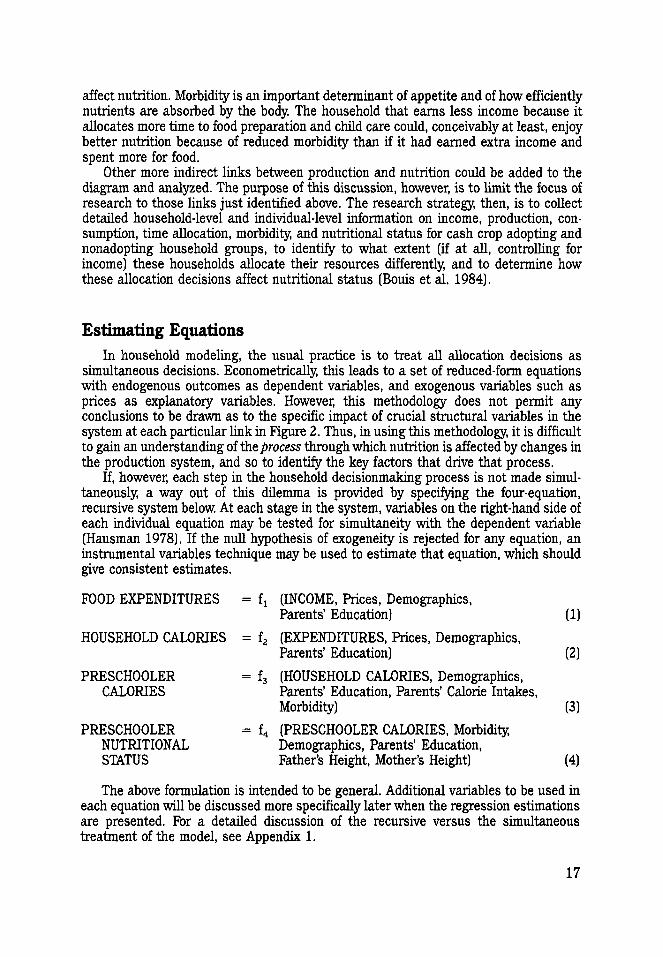
Estimating Equations

In household modeling, the usual practice is to treat all allocation decisions assimultaneous decisions. Econometrically, this leads to a set of reduced-form equationswith endogenous outcomes as dependent variables, and exogenous variables such asprices as explanatory variables. However, this methodology does not permit anyconclusions to be drawn as to the specific impact of crucial structural variables in thesystem at each particular link in Figure 2. Thus, in using this methodology, it is difficultto gain an understanding of the process through which nutrition is affected by changes inthe production system, and so to identify the key factors that drive that process.

If, however, each step in the household decisionmaking process is not made simul-taneously, a way out of this dilemma is provided by specifying the four-equation,recursive system below. At each stage in the system, variables on the right-hand side ofeach individual equation may be tested for simultaneity with the dependent variable(Hausman 1978). If the null hypothesis of exogeneity is rejected for any equation, aninstrumental variables technique may be used to estimate that equation, which shouldgive consistent estimates.

FOOD EXPENDITURES =

HOUSEHOLD CALORIES =

PRESCHOOLERCALORIES

PRESCHOOLERNUTRITIONALSTATUS

ix (INCOME, Prices, Demographics,Parents' Education) (1)

f2 (EXPENDITURES, Prices, Demographics,Parents' Education) (2)

f3 (HOUSEHOLD CALORIES, Demographics,Parents' Education, Parents' Calorie Intakes,Morbidity) (3)

f4 (PRESCHOOLER CALORIES, Morbidity,Demographics, Parents' Education,Father's Height, Mother's Height) (4)

The above formulation is intended to be general. Additional variables to be used ineach equation will be discussed more specifically later when the regression estimationsare presented. For a detailed discussion of the recursive versus the simultaneoustreatment of the model, see Appendix 1.

17

Sample Selection and Categorization of HouseholdsConceptually, the research strategy is simply to sample cash crop adopting (sugar)

and nonadopting (corn) households, but in the Philippine context the situations of land-owners, tenants, and landless laborers need to be compared and contrasted, both withinand across crop groups. In selecting a sample, an additional consideration was bias dueto adopter self-selection. In the hope of obtaining roughly comparable adopting andnonadopting groups, the survey area was extended beyond the vicinity of the mill toinclude households that did not have the opportunity to adopt sugar (due to prohibitivecosts of transporting the sugarcane to the mill) but shared a common growing environ-ment and cultural heritage with sugar-adopting households.

A short "presurvey" of 2,039 randomly selected households was undertaken,primarily to ask about present and previous occupations, crops being grown, andlandholdings. This served two purposes. First, it gave a picture of present employmentand land tenure patterns in the survey area and of how these patterns had changedsince the sugar mill was built. Second, it provided a frame for choosing a stratifiedsample of 510 households consisting of landowner, tenant, and landless agriculturallabor households within each crop group.

Only households (with at least one child under 60 months of age) that farmed lessthan 15 hectares were eligible for selection. Only households that characterized theprimary occupation (including wage income) of the head of household as either corn orsugar production were eligible for selection (except for a small target group of nonfarmhouseholds). Later analysis of the detailed survey data indicated that the respondents'characterizations of their crop and tenure status were quite accurate.

Four detailed surveys were undertaken in these households at four-month intervals,beginning in August of 1984 and ending in August of 1985. Four hundred and forty-eight households remained by the end of round 4. The loss of respondent householdswas due primarily to out-migration. Table 1 shows the topics covered in each of the foursurvey rounds.

For purposes of analysis, households were divided into 10 groups. Any householdcultivating an average of at least 1 hectare per round of any crop that produced anysugar at all was placed in one of three groups, "sugar owner," "sugar owner/renter(mixed)," or "sugar renter," depending on the proportion of total land cultivated thatwas owned and rented in. All other households cultivating an average of at least1 hectare per round were placed in one of four groups, "corn owner," "corn owner/sharetenant (mixed)," "corn share tenant," and "corn/other rent," depending on the propor-tion of total land cultivated that was owned, rented in on a share basis, or rented in on afixed-rate or other type of arrangement. Typically, land rented for sugar production wasrented in on a fixed-rate basis. For corn, the typical rental arrangement was for thetenant to pay a proportional share of the harvest to the landowner. The corn/other rentgroup includes households that rented in land primarily on a nonproportional basis,usually at a fixed rent.

The households in the remaining three groups, which cultivated less than 1 hectareof land, are characterized as "landless," although this is not strictly true for about halfthe households in these three groups. If income from nonagricultural sources wasgreater than agricultural wage income, households were placed in a group designated"other occupation." If agricultural wages were greater than nonagricultural income andincome from sugar wages was greater than agricultural wages from all other crops,households were designated as "sugar laborer." The remaining "corn laborer" house-holds had sugar wages that were less than half of total agricultural wages.

18

Table 1—List of topics covered by survey questionnaires, 1984/85

Block Topic* Explanation

A" General household informationB Parcels of landC Agricultural production recordD Sugar producer's questionnaireE Corn producer's questionnaireF Rice producer's questionnaireG Other crop producer's questionnaireH Agricultural wage laborI Other sources of incomeJ Backyard productionK Assets (rounds 1 and 4)

L Past income and assets (rounds 1 and 4)Mb Food expendituresN Nonfood expenditures0 Source of water and food preparation (round 1)Pb Preschool feeding practices (round 2)Q Reproductive history (round 1)

R Health services and nutritional knowledgeS Time allocation of wifeT" Anthropometry and morbidityIP Individual food intakeV Perceptions of and reactions to technological

change (round 4)

Demographics, education, migrationOwnership, tenure relationsSteps in production, input use, outputPostharvest processing, disposition

of output including revenuesfrom sales, loans, pastproduction history

By crop, by taskNonagricultural employment and transfersLivestock, fruits, vegetablesLand, buildings, farm implements, consumer

durablesBy employment category; access to landOne-month recallFour-month recallPrimary, secondary; cooking fuel, storageBreastfeeding, weaning practicesLive births, miscarriages, causes of children's

deathDoctors, paramedics; based on quiz24-hour recallMeasurement, two-week recall24-hour recallBy crop; reasons for adoption, nonadoption; input

use

Source: International Food Policy Research Institute-Research Institute for Mindanao Culture survey 1984/85."All topics were covered in each of the four survey rounds unless otherwise indicated.'Accomplished on first visit to households. Remaining blocks were covered during a second visit.

These criteria distributed the sample households so as to avoid cells with lownumbers of observations, while taking into account the complexity of the land-tenurerelationships that were found. Virtually all "sugar" households produced some corn,except for sugar laborer households that had no land at all.

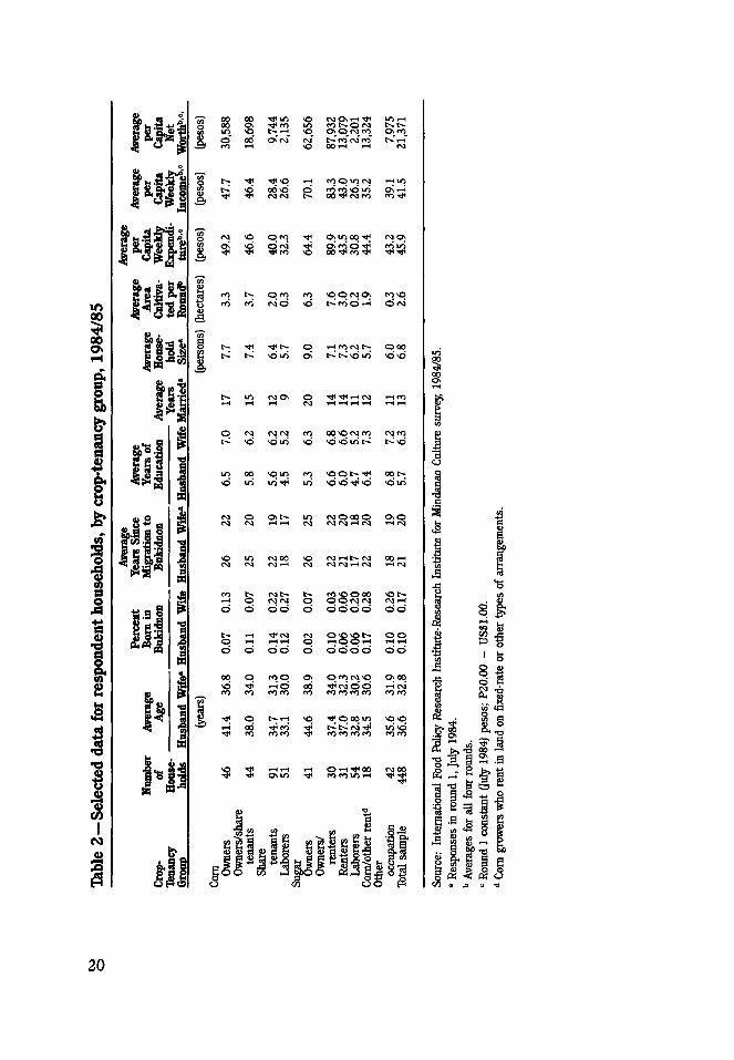
Table 2 presents selected characteristics that can be compared across the 10 house-hold groupings. The data show that the respondents are primarily a migrant population(typically from the Visayan Islands in the central Philippines). Those who own landtend to be older, to have migrated earlier, to have been married longer, and to have largerfamilies than tenant/renter households. These same relationships hold when comparingtenant/renter households with landless households and, although the data are notshown in lable 2, when comparing large farms with small farms. The level of educationis low, with respondents on average just having finished grade school.

As would be expected, incomes and expenditures of owner households are higherthan for tenant/renter households and higher for tenant/renter households than forlaborer households. At an exchange rate of P20 for US$1, per capita incomes of landlesslaborer households are roughly US$80 per year, those of corn owner households aboutUS$130, and those of sugar owner households approximately US$195.

In a comparison of like tenure groups across crops, although demographic variablesare quite similar, the one exceptional difference is that sugar farms are larger than cornfarms. This presents a problem in terms of the research strategy outlined above,wherein it was deemed necessary to sample adopting and nonadopting groups withsimilar resource bases. If the nutritional status of preschoolers in sugar households is

19

100o

i l l

J.'S:

1*8'

v© N O s H ^

s" a"

IT) T-H

VCO

t - • * Tl<>O .-I

pro fO OONO;

i-H fSI H f O

ro oq\poaro

co t-* N S t^ ro^OOOO voh-*-1 O C\3 r\l O pp<V3C^ OJ T-Ho d do d dodo oo

t^ f-1 Tt* N <M C O O t * O OO »—1 i—( T—( O i—* O O »-H H H

d d do d dodo do

oq p too o\^ 3 ^ 1 ^H < ^ QQ JH ^ ^ ^ ^ ^ ^ ^ ^ ^ ^co co co co co CO co co cO co co

CO COCO ^ CO CO CO CO COCO

CN100

20

better than the nutritional status of children in corn households, is the differenceexplained by having more access to land or by higher incomes that are possible fromsugar production? This turns out not to be a problem, since sugar-household childrenare not taller and do not weigh more than corn-household children once they reach theage of four. This difference in resource bases only reinforces a conclusion that, whilehigher income may be a necessary condition for improving the nutritional status ofpreschoolers, it is not a sufficient condition.

21

CHANGES IN LAND TENURE PATTERNSThe introduction of sugarcane production in Bukidnon apparently led to a significant

deterioration in the access to land. This is unfortunate for at least two reasons. First,because access to land is such an important determinant of income in rural areas in aland-constrained, labor-surplus country such as the Philippines (and the survey data tobe reported on later bears this out), income distribution has been skewed and lie plightof low-income groups has worsened. Second, if a larger proportion of the higher incomespossible from sugar production had gone to lower-income groups instead, the linkageswith other sectors of the rural economy would have been stronger, stimulating morelocal business and service activities, and so generating higher regional employment andeconomic growth (see Hazell 1983; Johnston and Kilby 1975; Mellor 1976; Ranis andStewart 1987).

1971 and 1980 Agricultural CensusesThe evidence that the expansion of sugar production has resulted to some extent

from a consolidation of smaller operational units comes from three sources: twoagricultural censuses conducted by the National Census and Statistics Office in 1971and 1980 (National Economic and Development Authority 1974,1985), the presurvey ofa random sample of 2,039 households in the study area in 1984, and the four surveyrounds. Table 3 shows the distribution of sugar and corn farms, by number of farms,area harvested, and size of farm, for 1971 and 1980 for the whole of Bukidnon Province.In 1971 sugar production was negligible, but it had expanded to more than 9,000hectares by 1980. Two-thirds of total sugar area was accounted for by farms larger than25 hectares, which constituted only 12 percent of all sugar farms.

By contrast, corn is a smallholder crop. In 1971 nearly three-fourths of corn farmswere less than 5 hectares and accounted for 40 percent of all corn area. Between 1971and 1980, corn area harvested increased by 51 percent and the number of corn farms by68 percent, implying (assuming no change in the cropping intensity) a modest reductionin average corn-farm size and a rapid expansion of population. By 1980 nearly50 percent of corn area was on farms of less than 5 hectares.

While these figures strongly suggest that smallholders participated only marginallyin the sugar expansion, it is not clear to what extent the expansion resulted from aconsolidation of smaller farms, if at all, or from the decision by large landowners toconvert to sugar production lands that they already owned and were either cultivatingthemselves or leaving fallow. The census data show that there was apparently someexpansion of total cropped area onto previously unused land during the 1970s.Unfortunately, the analysis that can be undertaken with the census is limited becausedata on operational farm size are not disaggregated by type of tenure; the census datarefer to the entire province of Bukidnon, while the surveys focus on the southern half ofthe province; and the census data cover only the period up to 1980 before the expansionof the sugar mill's capacity. The presurvey of 1984 offers more precise evidence.

22

Table 3—Percentage distribution of sugar and corn farms and area harvested inBukidnon Province, by farm size, 1971 and 1980

Crop/Year

Sugar19711980

Corn19711980

Sugar19711980

Corn19711980

LessThan1.00

Hectare

1.3

2.84.9

01

0.31.1

1.00-2.99

Hectares

14.9

41.141.1

2.3

16.125.1

Size

3.00-4.99

Hectares

of Farm

5.00-10.00

Hectares

10.00-24.00

Hectares

(percent of all farms)

15.629.722.5

(percent (

2.6

24.422.9

32.5

18.823.9

)f total area ]

io.o28.231.0

24.6

6.96.8

larvested)

17.621.814.1

More Than25.00

Hectares

11.7

0.60.8

68.1

9.25.8

TotalPercent

100.0

100.0100.0

100.0

100.0100.0

TotalAbsoluteNumber

(farms)

21951

37,62063,239

(hectares)

3209,365

162,607244,943

Sources: National Economic and Development Authority, 1971 Census of Agriculture (Manila: NEDA, National Censusand Statistics Office, 1974); and NEDA, 1980 Census of Agriculture (Manila: National Census and StatisticsOffice, 1985).

Note: Parts may not add to totals because of rounding.

Presurvey of 2,039 HouseholdsTable 4 presents the distribution of primary occupations of the heads of household

recorded from the presurvey. Eighty percent of the respondents identified themselves aseither landowners, tenants, or agricultural laborers. About 79 percent of these respon-dents directly employed in agriculture were engaged in corn production, while only7 percent were primarily employed in sugar production. Laborer households accountedfor less than 5 percent of households primarily engaged in corn or rice production, withthe percentage of landowners and of tenants about equal for each of these cereals.Among sugar producers, laborers accounted for nearly half of the households, with amuch lower percentage frequency for tenants and a somewhat lower percentagefrequency for landowners compared with corn and rice producers. The implication isthat if the same distribution of corn landowners, tenants, and laborers existed before theintroduction of sugar as now, some former corn landowners, but especially former corntenants, must have become sugar laborers.

Table 5, which presents data for the previous occupations of heads of householdspresently engaged in sugar production, shows that this is indeed the case. For amajority of households, land tenure status has not changed. However, 40 percent (21 outof 52) of households presently identified as sugar laborer households were corn owneror corn tenant households before the BUSCO sugar mill was built. Another 40 percent(22 out of 52) in-migrated to the area after BUSCO began operations (typically sugarlaborers from the islands of Negros and Panay, who were recruited by the sugarhacienda owners). Thus only about 15 percent of present sugar laborers (8 out of 52)came from the preexisting pool of corn laborers.

23

Table 4—Present primary occupation of heads of households, all municipalities,April 1984

Occupation

Direct agriculturalemployment

CornLandownerTenantLaborer

SugarLandownerTenantLaborer

RiceLandownerTenantLaborer

Other cropLandownerTenantLaborer

SubtotalTransportation-related jobsSkilled workersUnskilled workersSmall business/tradingOther (professional,

executive, police,technician, service,typist, clerk, jobless) —

Total

Number ofHousehold

Heads

1,28167057239

11644165617192718

59388

131,627

94624676

1342,039

Percent ofHousehold

Heads

62.832.928.11.95.72.30.82.78.44.53.50.42.91.90.40.6

79.84.63.02.33.7

6.6100.0

Percent ofTotal for

EachCrop

100.052.344.73.0

100.037.913.848.3

100.053.841.54.7

100.064.413.622.0

Source: International Food Policy Research Institute-Research Institute for Mindanao Culture presurvey ofrandomly selected households in southern Bukidnon Province.

Note: Parts may not add to totals because of rounding.

Except for the in-migrants, almost all households that switched to sugar productionhad previously been involved in corn production. It is especially important to note thatthe previous tenure distribution of those who switched from corn to sugar production isvery similar to the present tenure distribution of households primarily engaged in cornproduction.

Evidence from the Four Survey RoundsIn round 4 of the survey, respondents were asked detailed questions about changes

in their tenure status since the establishment of the BUSCO sugar mill. Table 6 is con-structed from these responses. All 448 of the round 4 households are included in Table6, not only households presently engaged primarily in sugar production as in Table 5.For purposes of comparison with Table 5, the tenure categories used are thoseattributed by the households to themselves, not the categorizations used later in thereport that are based on reported landholdings and sources of income.

Table 6 divides the respondents into four employment categories: those primarilyengaged in corn production; those primarily engaged in sugar production; those primar-

24

00

1

IaI

<OOONMO r O O N O

o O »-H O

O O O ro

lOMOOHO OOO<

r o O O O - H O OOOrO

I - H O O O

v 53

I

.gs

ON

-22 rt

-B .a

•S 13

•5 s.

' I S3

c^PQ

25

Table 6—Household employment and land tenure status during round 4 ofsurvey and before sugar mill operation, July 1985

Previous Status"

OwnerShare tenant/renterLaborerNonagricultural employmentNew household11

Total


Total


Total

OwnerShare tenant/renterLaborerKonagricultural employmentNew household11

Total

Owner

552121

1190

253000

28

366004

46

Present Status

Tenant Laborer

Households Engaged Primarily inCorn Production

5 0?8 32 50 0

14 8149 16

Households Engaged Primarilyin Sugar Production0 18 71 110 04 17

13 36

Households Engaged Primarily inAgricultural Production (No Crop Specified)

2 214 02 60 04 4

22 12

Households Engaged Primarilyin a lNonagricultural Occupation

Total

60122

91

63255

2618120

2177

402080

1280

4101

129

36

Source: International Food Policy Research Institute-Research Institute for Mindanao Culture survey, 1984/85.a Employment or land tenure status before the Bukidnon Sugar Company (BUSCO) mill began operations in 1977.b In-migrants to area after BUSCO sugar mill was built.

ily engaged in agricultural production, but who declined to specify a particular crop asdominant; and those primarily engaged in nonagricultural employment. ComparingTables 5 and 6, note that the percentage of present sugar laborers (who specified atenure status as a corn producer when BUSCO was established) who lost access to landis nearly equal between the two tables (21 out of 52 in Table 5 and 8 out of 19 in Tkble6). The percentages are also similar for present sugar landowners (2 out of 42 in Table 5and 3 out of 28 in Tkble 6) and for present sugar renters ( - 2 out of 16 for Tkble 5 and 1out of 9 for Tkble 6) who bettered their past tenure status.

Tkble 6 shows that 56 out of 64 households that became involved in corn productionafter the establishment of BUSCO were able to acquire access to land, so the overalltenure pattern remained stable over time (many older residents improved their statusfrom tenant to landowner, while newly married or newly resident couples embarked oncorn production in disproportionate numbers as tenants). For households primarily

26

engaged in sugar production, however, only 4 out of 21 newly married or newly residenthouseholds got access to land, and none as landowners.

A high percentage of households presently engaged primarily in nonagriculturalemployment who were married Bukidnon residents when BUSCO was established(14 out of 27) had lost access to land. Only one household moved in the other direction,from nonagricultural employment to corn production. The survey data, then, alsopresent a contrasting picture between sugarcane and corn production of relatively easyaccess to land for corn production and of a decline in access to land as sugarcane isadopted.

From Table 6, it is possible to identify 38 households whose tenancy statusimproved, 34 households whose tenancy worsened, and 236 households (with previousaccess to land) whose tenancy status remained the same. Sixty-seven newly in-migrantor newly formed households gained access to land. The remaining 73 households(including both old residents and new households) have never acquired access to land.

Analysis of the survey data by change in tenancy status shows that for householdsengaged in corn production the sizes of farms being converted to and taken out of comproduction appear to be in rough equilibrium. The average area cultivated by house-holds whose tenancy status was unchanged at 2.5 hectares is almost equal to theaverage area lost of the 25 households that reported a decline in tenancy status at2.4 hectares and to the average 2.8 hectares cultivated by the 26 households whosetenancy status improved. The size of the average corn farm appears, however, to havebeen decreasing over time, as the farms of new households at 1.6 hectares aredisproportionately tenant households, which tend to be smaller than owner corn farms.

The dynamics of change in farm size for sugar production appear to be quitedifferent. The average area cultivated by adopting households was about 5.5 hectares—more than twice the area cultivated by the average corn household. The average arealost by households whose tenancy status declined and whose land was converted tosugar production was only a third that size at 1.8 hectares.

Finally, in each month in which wages from sugar production were earned,respondents were asked to identify a farm-size category in which this labor wasperformed, ranging from a score of 1 for farms larger than 50 hectares to a score of 5 forfarms smaller than 5 hectares. An average score of about 4 was reported by therespondents, indicating that most of the off-farm sugar labor provided by our respondenthouseholds was hired in by farms of medium size relative to all farms, though smallrelative to those farms engaged primarily in sugar production.

Did sugar expansion occur on previously unused land? Certainly whatever expan-sion onto previously fallow land occurred on the largest sugar haciendas contributedlittle to the employment of local residents, who tended to be hired instead by relativelysmall sugar farmers.

Eighty of the sugar households who grew sugar during the survey (and had previousaccess to land) and whose tenancy status remained the same reported that in 1977 theygrew mostly corn and that only about 10 percent of their land was left fallow, apercentage similar to that surveyed during 1984-85. Over the same period, these80 households reported a 28 percent increase in the amount of land that theycultivated, an absolute increase of 1.3 hectares from 4.6 hectares in 1977. The farms ofsmallholder sugar adopters (small relative to all sugar adopters, large relative to theaverage corn-producing farm) increased in size as sugarcane replaced corn production.The evidence from households with access to land, then, supports a conclusion thatthere was some consolidation of existing operational farm units.

27

ConclusionAs already pointed out, land reform is central to the agricultural policy debate

presently taking place in the Philippines. In the context studied here, a kind of landreform in reverse has taken place with the introduction of export cropping. This raisesat least two important questions. The first is the empirical question (which is beyond thescope of the present study) of whether a similar deterioration in access to land has beenoccurring all over Mindanao, where various other export crops have been newlyintroduced.

Second, what are the forces driving this redistribution of land? The analysis thatfollows will show that these forces appear to be the declining productivity of corn lands,and the know-how and financial resources of the wealthier families, who are in a posi-tion to take advantage of a new income-earning opportunity.

28

COMPARISON OF THE CORN AND SUGARPRODUCTION SYSTEMS

This chapter compares the relative profitability of corn and sugar production. Anadditional objective is to disaggregate total labor inputs, not only by hired and familylabor, but also by labor performed by men, women, and children, in order to gain possibleinsights into changes in intrahousehold time allocation patterns that might be the resultof a switch to sugar production.

The Corn Production SystemDuring the postwar period up until the early 1970s, Bukidnon was a region of heavy

in-migration. New settlers typically homesteaded recently cleared rain forest. Conversa-tions with persons who migrated to Bukidnon before 1970 about past corn yields andagricultural wage rates invariably indicated a significantly declining trend in corn yieldsdue to loss in soil fertility, and lower shares of harvest paid to hired laborers over time.An attempt was made to measure these two trends in the detailed household surveys.

According to the respondents, corn yields have fallen dramatically over the past twodecades—more than 50 percent in an average of 13 years (Table 7). Similarly, sharespaid to harvesters have declined significantly, from one sack in every five harvested inthe mid-1960s to one sack in every eight by the time of the survey. The indicated trends,then, are very pessimistic: declining productivity and increasing land pressure.

Peak corn harvests occurred in July and December. The average growing cycle fromplowing to harvest was 3.3 months, so there is ample time to grow three crops a year.However, producing a third crop depends on rainfall at the onset of the relatively drymonths from March to May. Most of the respondents were able to produce two crops ayear. A few households produced three crops. Average yields were highest for the firstcrop, an average of 0.9 metric ton of shelled corn per hectare.1 Yields fell by 25 percentfor the second crop.

The average labor input per hectare per crop was 51 days. About two-thirds of thislabor input is provided by family labor and one-third by hired labor. There is a strongertendency for the family labor input per hectare to increase as farm size decreases thanfor hired labor to decrease with farm size. Consequently, labor inputs per hectare aresomewhat higher on small farms.

Tractors are used only on the largest farms, and these only sparingly. Landpreparation (plowing, harrowing, furrowing) accounts for about 20 percent of total laboruse, weeding (with carabao, by hand, or with sickle) almost 50 percent, harvestingabout 20 percent, and planting and fertilizing the remaining 10 percent. The onlystriking differences in labor inputs across household groups within particular tasksoccur for weeding by hand and weeding with a carabao, where there is an obviouspossibility of substitution between the two types of inputs. There is some tendency for

1 All tons in this report are metric tons.

29

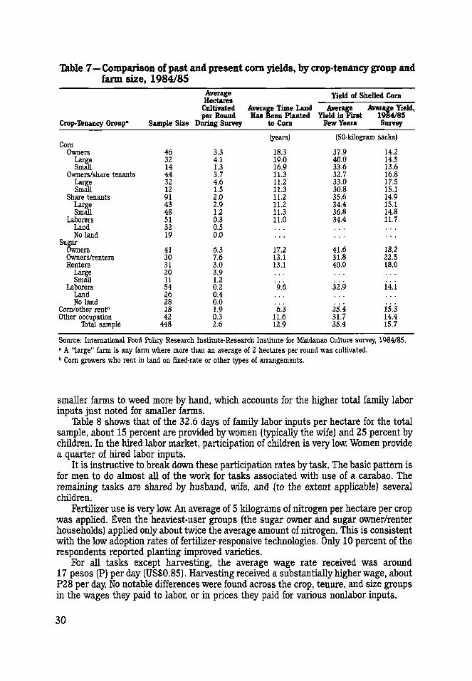
Table 7—Comparison of past and present corn yields, by crop-tenancy group andfarm size, 1984/85

Crop-Tenancy Group*

OwnersLargeSmall

Owners/share tenantsLargeSmall

Share tenantsLargeSmall

LaborersLandNo land

SugarOwnersOwners/rentersRenters

LargeSmall

LaborersLandNo land

Corn/other rentb

Other occupationTotal sample

Sample Size

463214443212914348513219

41303120115426281842

448

AverageHectares

Cultivatedper Round

During Survey

3.34.11.33.74.61.52.02.91.20.30.50.0

6.37.63.03.91.20.20.40.01.90.32.6

Average Time LandHas Been Planted

to Corn

(years)

18.319.016.911.311.211.311.211.211.311.0

17.213.113.1

9.6

6.311.612.9

Yield of Shelled Corn

Average Average Yield,Yield in First

Few Years1984/85Survey

(50-kilogram sacks)

37.940.033.632.733.030.835.634.436.834.4

41.631.840.0

32.9

25.431.735.4

14.214.513.616.817.515.114.915.114.811.7

18.222.518.0

14.1

15.314.415.7

Source: International Food Policy Research Institute-Research Institute for Mindanao Culture survey, 1984/85.a A "large" farm is any farm where more than an average of 2 hectares per round was cultivated.b Corn growers who rent in land on fixed-rate or other types of arrangements.

smaller farms to weed more by hand, which accounts for the higher total family laborinputs just noted for smaller farms.

Table 8 shows that of the 32.6 days of family labor inputs per hectare for the totalsample, about 15 percent are provided by women (typically the wife) and 25 percent bychildren. In the hired labor market, participation of children is very low. Women providea quarter of hired labor inputs.

It is instructive to break down these participation rates by task. The basic pattern isfor men to do almost all of the work for tasks associated with use of a carabao. Theremaining tasks are shared by husband, wife, and (to the extent applicable) severalchildren.

Fertilizer use is very low. An average of 5 kilograms of nitrogen per hectare per cropwas applied. Even the heaviest-user groups (the sugar owner and sugar owner/renterhouseholds) applied only about twice the average amount of nitrogen. This is consistentwith the low adoption rates of fertilizer-responsive technologies. Only 10 percent of therespondents reported planting improved varieties.

For all tasks except harvesting, the average wage rate received was around17 pesos (P) per day (US$0.85). Harvesting received a substantially higher wage, aboutP28 per day. No notable differences were found across the crop, tenure, and size groupsin the wages they paid to labor, or in prices they paid for various nonlabor inputs.

30

Table 8—Total labor inputs per corn crop, by family and hired labor, crop-tenancygroup, and farm size, 1984/85

Crop-Tenancy Group"

CornOwners

LargeSmall



Laborers

SugarOwnersOwners/rentersRentersLaborers

Corn/other rentb

Other occupationTotal sample

Men

19.818.522.918.715.327.319.416.921.924.7

15.711.818.820.517.724.319.1

Family Labor

Women

4.34.92.95.15.15.24.23.54.8

10.3

2.72.95.06.95.5

10.55.2

Children Men

(person-days/hectare)

5.66.04.96.54.3

12.07.99.16.8

11.3

11.76.2

15.016.54.12.48.3

16.917.914.310.411.77.2

10.09.1

10.86.0

12.819.613.59.0

17.716.412.5

Hired Labor

Women

5.25.44.83.63.83.14.74.84.73.3

5.05.97.22.36.38.34.9

Children

1.31.11.70.80.70.91.21.21.20.3

1.50.80.82.50.91.81.1

Source: International Food Policy Research Institute-Research Institute for Mindanao Culture survey, 1984/85.a A "large" farm is any farm where more than an average of 2 hectares per round was cultivated.b Corn growers who rent in land on fixed-rate or other types of arrangements.

The average production cost per hectare was P650. Of this, about two-thirds waspaid in cash and one-third in kind (mostly harvest wages, but in-kind payments alsoincluded meals for hired laborers engaged in other tasks). Wages (cash plus in-kind)accounted for about two-thirds of total expenses.

Per hectare in-kind wage payments did not vary a great deal across groups and farmsizes, so cash expenditures accounted for most of the differences across groups in totalcosts per hectare. Corn laborer and sugar laborer groups spent an average of less thanP200 cash per hectare per crop. Sugar households (apart from the laborer group)invested the largest amounts of cash, an average of P600 per hectare per crop.

All sugar households continued to produce some corn. Per capita consumption ofown-produced corn in sugar households (about 1.3 kilograms per capita per week) wasmuch lower than in corn households (about 2.0 kilograms per capita per week),although sugar households produced sufficient corn to have consumption levels equal tothose of corn households (Table 9). Sugar households preferred to purchase more rice inthe market instead. For corn households, per capita consumption of home-producedcorn on small farms was only marginally lower than on large farms, suggesting thathouseholds kept what they needed for home consumption and sold the remainder.

Labor for postharvest shelling, drying, and transport of com for marketing or formilling into grits was provided primarily by the family and added an average of 3.5 daysof total labor inputs per hectare. Analysis of marketing margins between farmgate andretail prices of corn and costs of having shelled corn milled into grits indicates thatfarmers who grow corn for own consumption save a premium of 25 percent (less storagelosses and interest costs) compared with selling their output and buying corn grits inthe retail market.

31

Table 9—Shelled corn production and consumption of own production, by crop-tenancy group and farm size, 1984/85

Crop-Tenancy Group1

ComOwners

LargeSmall



LaborersSugar

OwnersOwners/rentersRentersLaborers

Corn/other rentb

Other occupationTbtal sample

Production

7.08.14.4

10.713.23.98.4

10.26.91.3

4.96.05.20.77.81.15.3

Production Net Consumption Outof In-Kind Cost of Own Production

fkilograms/week/capita)

6.07.13.68.6

10.72.84.96.04.00.9

4.24.73.70.46.20.83.9

2.22.41.91.91.91.81.92.11.80.5

1.61.31.00.21.70.51.3

Share ofNet Production

Sold

(percent)

64674977803663694934

63747250622967

Source: International Food Policy Research Institute-Research Institute for Mindanao Culture survey; 1984/85.* A "large" farm is any farm where more than an average of 2 hectares per round was cultivated.b Corn growers who rent in land on fixed-rate or other types of arrangements.

Average returns to corn production axe a dismal PI,023 per hectare per crop(US$51; partly in cash, partly in the form of own-produced corn consumption). Sharetenants do worse than this average, since the share paid to their landlords has beensubtracted.

The Sugar Production SystemOne of the primary differences between production of corn and of sugar is the way

processing and marketing are organized. With corn, individual households may makeindependent decisions as to when to plant, harvest, and market their corn (subject, ofcourse, to rainfall patterns). With sugar, production must be coordinated among severalproducers so that milling capacity is as fully utilized as possible withoutoverproduction.

A second basic difference between production of the two crops is the length of thegrowing period, 3.3 months on average for corn for the sample households and12.0 months for sugar. For sugar, 12.0 months is only the average time betweenharvests, not between plantings, since sugar may be ratooned. There are substantiallyhigher input costs for the plant crop than for successive ratoons.

The sugar milling season begins in late October and ends in late July. The sugarcontent of the cane tends to be highest in March and April, when there is less rain. Mostfarmers would prefer to plan for harvesting then, but the mill prefers to process canemore or less evenly throughout the milling season.

32

The problem of coordinating the planting and harvesting of all contracted hectaresis resolved ingeniously through a system that revolves around the bagon (wagon), ormetal carrier, that sits on a truck bed and is lifted by cranes to dump the cane onto aconveyor belt at the mill. One bagon can service roughly 40 hectares if it is filled tocapacity and delivered each day that the mill is in operation during the nine-month mill-ing season. The mill assigns one bagon to each group of farmers with sugar contractsthat total 40 hectares (operators of large farms would have several bagons at theirdisposal). Each group of smallholder farmers, then, must arrange a mutually agreeableschedule for utilization of that bagon capacity during each day of the milling season.

Several of the sugar household respondents had no contracts with the mill butworked out deals with growers who did not want to plant sugarcane up to the maximumof their contracted hectares ("deficit" producers).

A typical arrangement might be for a surplus grower to sell sugarcane to the deficitgrower at a certain rate per truckload of cane. The deficit planter proceeds to thesurplus grower's field with a truck and laborers, who cut and load the cane into thedeficit planter's bagon. The deficit grower, who undertakes the expense of harvestingand hauling the cane, brings the cane to the mill as if it were his own production. Thistype of arrangement presents no particular problem for operation of the overall systemjust outlined.

When the cane is brought to the mill, it is weighed and a sample is taken todetermine its sugar content. The grower is paid the National Sugar Trading Agency(NASUTRA, the government agency to which mills were required by law to sell theiroutput) price for 60 percent of the sugar equivalent and the remaining 40 percent isretained by BUSCO. The grower is also paid a transportation rebate by the mill for thehauling of the mill's 40 percent of the cane. This rebate is paid on a kilometer and tonbasis, so that farms farther away from the mill get a higher rebate. However, whilecontracts are given to farms outside of a 20-kilometer radius from the mill, rebates arepaid only up to a maximum of 20 kilometers.

In the past growers were paid, usually within a month of depositing a truckload ofcane at the mill, a single payment for both sugar and trucking rebate. Toward the end ofthe survey period, payments were delayed three months and more. Since a single growermay deliver several truckloads throughout the milling season, payments are staggeredthroughout the year. Some growers have large enough operations that it is moreprofitable to buy and use their own trucks to haul their cane. The growers in the samplewere small enough that in all cases they hired private truckers to haul their cane.

Table 10 shows that average sugarcane yields were nearly identical across tenuregroups. There was an almost uniform drop in yields across tenure groups between thetwo milling seasons recorded in the survey rounds.

The average total labor input per hectare was 109 days. The proportion of familylabor in total labor for all groups was about one-third, with the exception of the sugarowner/renter group, which hired nearly 90 percent of its total labor inputs. Weedingaccounted for 45 percent of all labor inputs and harvesting for 35 percent. Landpreparation accounted for a low percentage of total labor inputs, partly because of thepractice of ratooning, but also because tractor usage is much higher than for corn.

As indicated in Table 11, women contributed 9 percent of family labor and 11 percentof hired labor for sugar, lower percentages than for corn. As with family labor for corn,women are almost entirely excluded from tasks involving a carabao and participate,along with several children, in all other tasks except preparing the ratoon. In the hired

33

Table 10—Sugar yields, by crop-tenancy group and milling season, 1984/85

By Milling Season

Crop-Tenancy Group

Sugar ownersSugar owners/rentersSugar renters

Large'Small

Tbtal sample

1983/84MillingSeason

59.553.467.882.050.859.1

1984/85MillingSeason

(metric tons40.637.335.738.531.638.3

Two MillingSeasons

Combined

of cane/hectare)49.843.248.354.839.647.2

AverageRatoonNumber

1.71.81.61.61.61.7

Source: International Food Policy Research Institute-Research Institute for Mindanao Culture survey, 1984/85.a A "large" farm is any farm where more than an average of 2 hectares per round was cultivated.

Table 11—Tbtal labor inputs per sugar crop, by crop-tenancy group and familyand hired labor, 1984/85

Crop-lenancy Group

Sugar ownersSugar owners/rentersSugar renters

Large"Small

Total sample

Men

20.78.5

19.515.125.416.5

Family Labor

Women

3.80.63.54.22.62.7

Children Men

(person-days)20.92.75.45.55.3

11.9

67.777.652.553.151.868.2

Hired Labor

Women

9.09.16.35.96.88.6

Children

1.40.50.40.80.00.9

Source: International Food Policy Research Institute-Research Institute for Mindanao Culture survey, 1984/85.* A "large" farm is any farm where more than an average of 2 hectares per round was cultivated.

labor force, women's participation rates fall when compared with corn, primarilybecause they are excluded from harvesting.

Average fertilizer usage per hectare per crop is between two and three times higherfor sugar than for corn, although the duration of the growing cycle is much longer forsugar. The sugar owner/renter group uses the most fertilizer, 16 kilograms of nitrogenper hectare, which in absolute terms is still quite low

Wage levels for all tasks are similar to those paid to corn laborers. There are not anyobvious patterns of wage differentials across tenancy groups. As with corn, the wagepaid for harvesting is substantially higher than for other tasks and about equal to thewage paid to corn harvesters at P27 per day.

Average expenditure per hectare for all household groups was P2.200, virtually allof which was paid out in cash. Thus, not only are production expenses much higher percrop per hectare than for corn, but a much higher proportion is paid out in cash. As withcorn, about two-thirds of total expenses are paid out as wages. Total expenditures forthe sugar owner/renter group are somewhat higher than average, lbtal expenditures forthe small sugar renter group are well below the average due to lower levels of nonlaborinputs.

Plant crop expenses are, on average, about P800 more per hectare than ratoon cropexpenses. If fertilizer applications had been constant across plant and ratoon crops, thisdifferential would have been larger.

34

The price paid for sugar changed three times during the two milling seasons. At thebeginning of the 1983/84 milling season, the price per picul2 of sugar stood at P85.Toward the end of the milling season, this price was raised to P96. By the beginning ofthe 1984/85 milling season this price had increased to P107, and at about the middle ofthe milling season the price increased sharply to PI71 per picul (the result of adevaluation of the peso).

Average returns of P4.500 per hectare per crop for sugar were well above those forcorn. As with corn, landowners do better than renters because of the variable cost-accounting method used. Economic returns to corn and sugar production are examinedmore closely in the following section.

Comparison of Profits and Labor Allocation PatternsTable 12 shows net revenues for corn and sugar (calculated on a variable cost basis)

and net profits per hectare after subtraction of imputed values for family labor, inputsfor carabaos owned by the household, interest on cash inputs, and rents on owned land.Except for land prices, the introduction of sugar did not affect the local prices of theseinputs, or the output price for corn. Before finally subtracting an imputed value forowned land, a subtotal is calculated in which imputed values for family labor, owned-carabao inputs, and interest on cash have been subtracted from net revenues.

For corn laborers this subtotal is negative. This implies that these households couldhave had a higher income by hiring out their family labor and carabaos on the labor andcarabao rental markets rather than devoting these inputs to corn production—assuming that employment is readily available if desired. Corn share tenants barely dobetter than break even, compared with the alternative of employment in the labormarket.

In general, corn production by sugar households earns the highest returns net offamily labor, carabao inputs, and interest on cash. The corn mixed tenancy group doesnearly as well, but the pure corn landowner group does less well. Net profits are higherfor sugar relative to corn, compared with net revenues for sugar relative to corn, sincefamily inputs are greater for corn.

The final calculation shown in Table 12 is to subtract imputed rental values onowned land. Several negative entries in the final column for corn indicate that thesehouseholds would have done better to rent out their land at the assumed rate (and enterthe labor market) rather than to have undertaken corn production. This is not to saythat farmer behavior is economically irrational. Yields and prices obviously cannot bepredicted with complete accuracy, and some value may be attached to working foroneself rather than for someone else. But the low average value (a net profit of only P93per hectare per crop) for the total sample indicates what a marginal activity cornproduction has become over time for smallholders.

Net profits for corn and sugar for the sugar owner/renter and sugar owner groupsare roughly equal after doubling corn profits to take account of the two crops per yearthat can be planted to corn. These households would appear to have done a good job ofallocating resources between sugar and corn production so as to have equalizedmarginal returns in both activities. This does not appear to be the case, however, for

: One picul equals 60.477 kilograms.

35

I00ON

1

Jfi;

I 1!

1I

N <i-H i -^ i—l

I I I

Oo

00 H » OT-H vO O i-4f O f O N t~- 00 (M a*ON

O^OOO O O v O O O O N N 1 * ^ < O ON H N 0O • * H OMC • * Oi ^ H f v a ^t*^ t*1* t^ ^O ^) QQ \ > * ^ t ^ 00 t*1™ ^D 00

O!l0rHC^-O^p0 Oi - t^rO^rgt-»00t^vO \Qw)O

i'\t

£

q> H M

c t3 9

1sljs

. • s .

1 «•) O

36

sugar renter households, which seem to have overinvested family labor in cornproduction.

Table 13 shows average labor inputs for corn and sugar production. The corn figureshave been doubled to take account of the two corn crops that are harvested for eachsugar crop. Corn and sugar production use almost identical amounts of total labor. Aspreviously mentioned, however, the mixes of family and hired labor, and of men's,women's, and children's labor are quite different. While the substitution of hired forfamily labor in switching from corn to sugar production is perhaps marginally over-stated in Table 13 due to the larger farm sizes of the sugar households, most of thissubstitution would appear to be related to the particular characteristics of the corn andsugar technologies themselves. As a proportion of total labor inputs, harvesting is abouttwice as important for sugar production as for corn production (both technologies useprimarily hired labor for this step in the production process). This explains more thanone-half of the increase in hired labor for sugar production. Tasks involving carabaosand postharvest processing explain more than one-half of the increase in family laborfor corn production. Tractor use, which does not appear to be strongly related to farmsize, is commonly used for land preparation in sugar production. Women's participationin household production declines dramatically with a switch from com to sugarproduction, from 12.4 days per hectare for corn to only 2.7 days for sugar.

Other Sources of IncomeThe following chapters will analyze how incomes generated from the production of

corn and sugar are spent and how time allocation and expenditure decisions affect thenutrition of preschoolers. Before proceeding, however, it is important to keep in mindthat the sources of income for these households are very diverse, especially forhouseholds with access to land.

Table 14 shows the percentage distribution of various sources of income, disaggre-gated by expenditure quintile and by crop and tenure group. For corn households with

Table 13—Labor inputs for corn and sugar, by family and hired labor, 1984/85

LaborGroup Corn* Sugar6

Family laborMenWomenChildren

Hired laborMenWomenChildren

Total laborMenWomenChildren

Source: International Food Policy Research Institute-Research Institute for Mindanao Culture survey, 1984/85.Note: Labor inputs shown are for the total survey sample and include postharvest processing.a Com figures are for two crops.b Sugar figures are for one crop.

37

70.040.212.417.439.226.011.02.2

109.266.223.419.6

(person-days/hectare)31.016.52.7

11.977.668.28.60.9

108.684.711.312.8

f:

!00

s

1

oI

888888 8888888888

o\ oo oo t- t -

>^ HS*O^OON8 8 '

HOvXOfO CO N fv]

-S9

I ! •§

I"S

m g j2

•3

g

ill

38

access to land, profits from corn production account for only about a third of totalincome. Sugar households with access to land derive about the same proportion of theirincome from sugar production.

For both crop groups with access to land, income from nonagricultural sources con-tributes a quarter of total income. Backyard livestock, vegetable, and fruit production isa more important component of income for corn households with access to land than forsugar households with access to land, partly because livestock production is acomplementary activity to corn production.

Rice and corn production account for about 15 percent of income for sugarhouseholds with access to land. Crops other than sugar, rice, and corn do not figureprominently for these households. For corn households with access to land, rice andother crops provide significant proportions of income for owner and owner/renterhouseholds but not for share tenant households.

Landless laborer households, whether corn or sugar, are the most dependent on asingle source of income, agricultural wages, which constitutes from two-thirds to three-fourths of total income. For these households, backyard production, at roughly 15 per-cent, is the second largest component of income.

39

FOOD EXPENDITURES AND CALORIE INTAKES

The links between income and food expenditures at the household level, betweenfood expenditures and household calorie intakes, and between household calorie intakesand preschooler calorie intakes for corn and sugar families are examined in this chapter.For reasons developed at length elsewhere (Bouis and Haddad 1989), total expendituresand calorie intakes derived from the 24-hour recall of foods consumed by a family arebelieved to give the best indication of the effect of increases in purchasing power on im-proved calorie consumption at the household level. A commonly followed alternativewould have been to estimate the relationship between calorie availability (derived fromfood-expenditure information) and total expenditures.

Appendix 2 contains a discussion of how data on incomes, expenditures, nutrientavailability, and nutrient intakes were collected, which data are more reliable, and howthese variables are related empirically. See Table 26 for estimates of the incomeelasticities based on the two-way relationship shown in Table IS. See Appendix 3(Tables 27-29) for descriptive statistics of the variables used in the following analysesand for the results of various structural and exogeneity tests.

Food Expenditures as a Function of IncomeTable 15 presents data for per capita income, total expenditures, food expenditures,

per adult-equivalent calorie availability, and calorie intakes disaggregated by incomequintile, total expenditure quintile, and crop-tenancy group. As expected, food budgetshares decline and household calorie consumption, increases with income.

Sugar households purchase an average of about 15 percent more of their food in themarket than do corn households, with proportions between own-produced food andmarket purchases invariant with tenure status. Conversely, about 15 percent more ofcorn-household food purchases come from their own production. This is not invariantwith tenure status, as households with access to more land produce a higher percentageof their own needs. Laborer households make up for a lower home production per-centage with higher percentages of in-kind wages.

Much of the difference between corn and sugar households in the percentagedistribution of market purchases can be explained by differences between the twogroups in their purchases of rice and corn, the two main staples. As indicatedpreviously, sugar-household purchases of rice in the market are higher than corn-household purchases. Prices paid for corn grits and rice do not vary by income group.An F-test indicates that the marginal propensity to consume rice out of income issignificantly higher for sugar households than for corn households.

The results of estimating the relationship between income and food expenditures aregiven in Table 16. The coefficients on the income terms are positive and significant forall three samples (corn households, sugar households, and the combined sample). Outof each additional peso of income, the marginal propensities to spend for food are49 centavos for the whole sample, 52 centavos for corn households, and 39 centavos forsugar households. In accordance with Engel's law, the higher-income sugar households

40

Table 15—Income, expenditures, and calorie availability and intake, by incomeand expenditure quintiles and crop-tenancy group, 1984/85

Group

Incomequintile8

12345

AllExpenditure

quintile"12345

AllCrop-tenancy group

CornOwnersOwners/share tenantsShare tenantsLaborers


PerCapitaIncome

13.121.929.841.4

101.741.7

21.925.428.545.887.641.7

35.247.746.428.426.652.270.183.343.026.5

TotalExpendi-

tures

(pesos/week)d

30.036.639.748.176.246.2

21.829.838.050.091.946.2

41.449.246.640.032.353.564.489.943.530.8

FamilyFood

Expendi-tures

24.026.628.533.343.231.1

17.223.428.834.851.731.1

29.332.730.429.624.933.739.347.530.024.0

FoodBudgetShare"

(percent)

807372695767

797976705667

71666574776361536978

CalorieAvail-

ability1'

(per

2,1702,2372,3212,6392,8262,439

1,7902,1432,4112,6663,1932,439

2,3752,4452,3682,4052,2662,5342,6553,1482,3502,208

CalorieIntake0

day)

2,2662,3132,3362,4332,4432,358

2,1082,2882,3842,4392,5752,358

2,3722,3872,3292,4122,3262,3432,3862,4472,3712,237

Source: International Food Policy Research Institute-Research Institute for Mindanao Culture survey, 1984/85.Note: Parts may not add to totals because of rounding." Food budget share = family food expenditures/total expenditures; shares are weighted by total expenditures for

individual households.b Per adult-equivalent, derived from food expenditures.c Derived from 24-hour recall of foods consumed.d 1984 pesos.• Quintile 1 is the lowest rank and 5 the highest.

spend a lower proportion of their incremental income on food. However, the range of thecorresponding elasticities, 0.65, 0.63, and 0.57, is smaller. Food expenditures riserapidly with income.

The test for equality of coefficients across corn and sugar households gave anF-value of 4.26, which is above the critical value. Changes in demand for householdlabor between sugar and corn production, especially for women, changes in demandpreferences for rice and corn, and differences in percentage of food purchased in themarket could all account for this result.

Calorie Intakes as a Function of Food ExpendituresCalories purchased per peso decline with increasing income, reflecting the declining

share of staples in the diet as higher-income households seek more variety in what theyeat. The food-expenditure data indicate that households in the highest expenditure

41

Table 16—Regression results for the relationship between income and foodexpenditures

Variable

(Constant)LNYMOTHEDFATHEDMOTHAGEFATHAGENUTRSC1PRCORNPRRICEPCTHOMEPOPDENADEQVHHRD1RD2RD3

Marginal propensityto spend for food

Food expenditureelasticity withrespect to income

AllHouseholds

-25.1521020.38670

0.91819-0.41277-0.32516

0.11586-0.43354

0.82957-1.38213

0.00253-0.02133-0.39700

4.142430.798261.59086

R 2 =

F =N =

(-4.38)(16.90)*

(5.08)*(-2.35) '(-3.25)*

(1.49)(-3.02)*

(1.14)(-2.41)*

(0.15)(-2.33)*(-1.48)

(3.70)*(0.64)(1.30)

: 0.362•• 6 5 . 3 2: 1,624

0.49

0.65

CornHouseholds

-15.5392018.492300.66936

-0.71002-0.52139

0.18369-0.59274-0.11026-0.45116

0.02339-0.01569-0.17440

5.281863.400792.26638

R2 =

F =N =

(-2.04)(9.74)*(2.86f

(-2.68)*(-4.10)*

(1.87)(-3.19)*(-0.13)(-0.62)

(1.08)(-1.34)(-0.45)

(3.81)*(2.15)*(1.48)

0.28025.36

928

0.52

0.63

SugarHouseholds

-28.4514019.08450

1.292990.601850.27850

-0.17939-0.22091

1.78659-3.53981-0.04679-0.00951-0.81660

1.68067-3.40899

0.54071

R 2 =

F =N =

(-3.26)(13.14r

(4.57)*(2.55)*(1.78)

(-1.46)(-0.96)

(1.53)(-3.98)*(-1.82)(-0.64)(-2.33)*

(0.99)(-1.82)

(0.29)

= 0.476= 36.88

624

0.39

0.57

Notes: The dependent variable is food expenditures per capita per week, t-statistics are in parentheses.•Significant at the 0.05 level.Definitions of variables:

LNY = predicted natural logarithm of income, in pesos per capita per week;MOTHED = years of formal education of the mother;FATHED = years of formal education of the father;MOTHAGE = age of mother in months;FATHAGE = age of father in months;NUTRSC1 = measure of the nutritional knowledge of the mother;PRCORN = quality-adjusted real price of corn;PRRICE = quality-adjusted real price of rice;PCTHOME = percentage of food expenditures coming from own-farm production;POPDEN = population density of the muncipality;ADEQVHH = number of household members expressed in adult-equivalents; andRD1,RD2,RD3 = zero-one dummy variables for round.

quintile spend 60 percent more than those in the lowest expenditure quintile for equalamounts of calories.

Table 17, which disaggregates food expenditures by five broad food groups, indicatesthe types of calorie-expensive foods the higher-income groups in the sample demand.Overwhelmingly, it is the meat category that increases its share with income as thestaple share declines. The category of fruits, snacks, desserts, and beverages increasesits share with income, although the percentage share remains low. The shares of theremaining two food groups remain nearly constant with rising income.

The regression results in Table 18 show that household calorie intakes increasepositively and significantly as food expenditures increase. At mean food expenditurelevels, each extra peso spent for food increased household calorie intake (per adult-equivalent) by only about 90 calories at the margin for the sample as a whole, compared

42

Table 17—Allocation of weekly per capita food expenditures, by food group,expenditure quintile, and crop-tenancy group, 1984/85

Group

Expenditure quintile"12345


ComOwnersOwners/share tenantsShare tenantsLaborers


Staples

615652453748

49454750564642404856

Meat,Eggs/Fish

202527313930

28313129233135363024

Vegetables,Legumes

Fruits,Snacks,

Desserts,Beverages

(percent)

555565

5455555565

789

111210

1013999

101112109

CookingIngredients

778877

7788777777

All

100100100100100100

100100100100100100100100100100

Source: International Food Policy Research Institute-Research Institute for Mindanao Culture survey, 1984/85.Note: Averages are weighted by food expenditures for individual households.a Quintile 1 is the lowest rank and 5 the highest.

with more than 400 calories purchased on average by a peso spent on food. Theestimated household calorie intake elasticities with respect to food expenditures are0.17 for the sample as a whole and 0.15 and 0.21 for corn and sugar households,respectively. Testing for the equality of coefficients across corn and sugar groups, anF-value of 0.79 does not reject the null hypothesis.

Direct Estimation of the Calorie-Income ElasticityCalorie-income elasticities for the entire sample of 1,624 observations have been

directly estimated using four econometric techniques (ordinary least squares, instru-mental variables, and two techniques designed to take account of unobservedhousehold-specific effects; a detailed presentation is provided in Bouis and Haddad1989). The instrumental variable technique gave a calorie-income elasticity estimate of0.11, and the two fixed-effect techniques gave estimates of 0.06 and 0.05, using calorieintakes and total expenditures as dependent and explanatory variables, respectively.These estimates, then, are nearly identical to the 0.11 estimate derived using the two-step procedure outlined above (obtained by multiplying 0.65 and 0.17) and suggest thathousehold unobserved effects are empirically relatively unimportant in this instance.

The expenditure behavior indicated by the regression results reveals a high degreeof leakage between higher incomes and increases in calorie intakes at the householdlevel. The striking conclusion is that as incomes double, household calorie intakesincrease by only about 10 percent for both corn and sugar households (less than10 percent if the panel estimates are used).

43

Table 18—Regression results for the relationship between calorie intakes andfood expenditures

Variable

(Constant)LNFFEXMOTHEDFATHEDMOTHAGEFATHAGENUTRSC1PRCORNPRRICEPCTHOMEPOPDENADEQVHHRD1RD2RD3

AllHouseholds

1,699.20348399.57051-6.55484

-10.29226-1.00478-3.82640

9.00880-40.57495

25.921910.65529

-2.03446-34.17901160.01210

5.53448-117.68181

R2 =F =N =

Calories purchased foreach additional pesospent on food

Household calorieintake elasticitywith respect tofood expenditures

(7.15)(9.80f

(-0.81)(-1.44)(-0.24)(-1.11)

(1.54)(-1.27)

(1.07)(0.92)

(-5.05f(-2.95)'

(3.22)*(0.10)

(-2.18)*

0.12516.431,624

89.8

0.17

CornHouseholds

1,572.79891348.18092

4.39447-9.53054-0.71330

0.039819.91045

- 7.1056322.964620.73085

-1.75213-48.58973207.05062

-47.53876-139.32955

R2 =F =N =

(4.65)(5.85f(0.38)

(-0.90)(-0.12)

(0.01)(1.28)

(-0.17)(0.67)(0.71)

(-3.06f(-2.69)'

(3.00)*(-0.61)(-1.85)

0.1178.60928

83.1

0.15

SugarHousehol

1,900.12249486.02863

-17.99340-13.14178

-6.58987-5.12551

4.41642-93.01054

39.972451.31968

-2.76975-19.60127116.2761083.46194

-100.18397

R2 =

F =N =

ds

(5.14)(7.95f

(-1.43)(-1.27)(-0.97)(-0.96)

(0.45)(-1.81)

(1.04)(1.17)

(-4.25f(-1.28)

(1.56)(1.01)

(-1.23)

0.1769.27624

100.8

0.21

Notes: The dependent variable is household calorie intake per adult-equivalent per day. t-statistics are inparentheses.

•Significant at the 0.05 level.Definitions of variables:

LNFFEX = natural logarithm of food expenditures, in pesos per capita per week;MOTHED = years of formal education of the mother;FATHED = years of formal education of the father;MOTHAGE = age of mother in months;FATHAGE = age of father in months;NUTRSC1 = measure of the nutritional knowledge of the mother;PRCORN = quality-adjusted real price of com;PRRICE = quality-adjusted real price of rice;PCTHOME = percentage of food expenditures coming from own-farm production;POPDEN = population density of the muncipality;ADEQVHH = number of household members expressed in adult-equivalents; andRD1,RD2,RD3 = zero-one dummy variables for round.

Preschooler Calorie Intakes as a Function of Family IntakesTable 19 presents average calorie adequacy ratios for various age groupings by

expenditure group and crop-tenancy group. These ratios are computed by dividingactual calorie intakes (taken from the 24-hour recall of individual food intakes) by therecommended calorie intakes for the appropriate age and sex (Food and NutritionResearch Institute 1984). Only preschoolers for whom breastfeeding has already beenstopped are included in the table, because data were not collected on calorie intakesfrom breast milk. Consequently, currently breastfed children were also excluded fromthe regressions reported on below and in the following chapter.

44

Q0'-HO\'-tin'-i rooo ^NOOMt^mrOfO

00

i1

I

"34>

I

a>

00 OO

•8

II,f

45

Table 19 shows that preschoolers on average are consuming only about 75 percentof their recommended daily intakes, while adults are consuming slightly above theirrecommended levels. Comparing calorie adequacy ratios across the various crop-tenancy groups, preschoolers in corn households consume more calories than sugar-household preschoolers. While the difference is not large, it is still surprising in view ofthe higher incomes in sugar households.

Table 20 presents the regression estimates for preschooler calorie intakes as afunction of household calorie intakes. For all three samples, the household calorie intakewas found to be a positive and significant determinant of preschooler calorie intake. Atthe margin, calories are distributed more or less equally among household members, in-creasing the percentage of household calories going to preschoolers, who consumebelow average household levels. For the whole sample and subsamples of corn and

Table 20—Regression results for preschooler calorie intakes as a function ofhousehold calorie intakes

Variable

(Constant)HCALAEQRATIOPARMOTHEDMOTHAGENUTRSC1CHILDCRESICKSEXACCAGEAGESQADEQVHHRD1RD2RD3

AllHouseholds

263.423990.82028

-1,483.48814 (16.796551.03590

-3.428590.32042

-81.7087165.9860943.84393

-0.5454849.24556

-2.93130-65.62428

-110.98226

R2 =F =N =

Preschooler calorie intakeelasticity with respect tohousehold calorie intake

(1.12)(30.86)*

-14.01)*(2.26)*(3.37)*

(-0.55)(1.63)

(-1.90)(1.73)(4.84)'

(-4.56)*(3.61)'

(-0.06)(-1.23)(-2.08)*

0.76999.08

975

1.18

CornHouseholds

530.870800.84577

-1,588.4631217.668451.02134

-13.817240.51105

-137.8729945.6423439.98655

-0.5277560.88718

-47.44410-94.31894

-110.95572

R2 =

F =N =

(1.69)(25.52)*

(-11.22)*(1.93)(2.68)*

(-1.86)(2.04)*

(-2.57)*(0.96)(3.27)'

(-3.32)*(3.35)*

(-0.71)(-1.39)(-1.65)

0.79268.91

587

1.20

SugarHouseholds

98.994750.77578

-1,320.443085.117380.79280

25.155190.05842

38.3826272.8092235.74011

-0.3590034.9433060.91730

-13.65748-106.97079

R2 =F =N =

(0.26)(16.68)*

(-7.57)*(0.35)(1.46)(2.11)*(0.18)(0.51)(1.07)(2.45)*

(-1.81)(1.62)(0.65)

(-0.15)(-1.17)

0.56730.90

345

1.17

Notes: The dependent variable is preschooler calorie intake per adult-equivalent per day. t-statistics are inparentheses.

•Significant at the 0.05 level.Definitions of variables:

HCALAEQ = household calorie intake per adult-equivalent per day;RATIOPAR = ratio of average of father's and mother's calorie intake per adult-equivalent over

the household calorie intake per adult-equivalent;MOTHED = years of formal education of the mother;MOTHAGE = mother's age in months;CHILDCRE = minutes spent by mother in child care in previous 24 hours;NUTRSC1 = measure of nutritional knowledge of the mother;SICK = zero-one dummy for reporting sickness in previous two weeks;SEX = 0 = female, 1 = male;ACCAGE = age of preschooler in months;AGESQ = age of preschooler squared;ADEQVHH = number of household members expressed in adult-equivalents;RD1,RD2,RD3 = zero-one dummy variables for round.

46

sugar households the estimated preschooler calorie-intake elasticities with respect tohousehold calorie intakes are 1.18, 1.20, and 1.17, respectively.

The F-test for equality of coefficients between the corn and sugar householdsindicated that the coefficients were significantly different for the two subsamples.Discussion of the reasons for this particular result will be postponed until differences inmothers' time allocation patterns between corn and sugar households are discussed inChapter 7.

Multiplying the calorie-income elasticities reported in the previous section by thecited elasticities of 1.18,1.20, and 1.17 gives the percentage increase in preschooler in-takes over the percentage increase in income, or 0.13, 0.11, and 0.14 for the wholesample, corn households, and sugar households, respectively. Because preschoolersstart off so far below their recommended calorie intakes, though distribution isrelatively equitable at the margin, even high-income households would have to realizesubstantial percentage increases in income for the calorie intakes of preschoolers toreach their recommended levels, given these low elasticity values.

47

HEIGHTS AND WEIGHTSOF PRESCHOOL CHILDREN

Anthropometric data on height and weight were collected in each of the four surveyrounds for all individuals present in the household at the time of the interview. In thischapter the data for preschoolers are presented, and the effects of calorie intakes andseveral nonfood variables on their heights and weights are analyzed. The standardsagainst which heights and weights are compared are the United States National Centerfor Health Statistics references for a healthy U.S. population.

Table 21 presents Z-scores for height-for-age, weight-for-age, and weight-for-heightfor all preschoolers, disaggregated by age and expenditure quintile. The height-for-age

Table 21—Z-scores for height-for-age, weight-for-age, and weight-for-height ofpreschoolers, by age and expenditure quintile, 1984/85

ExpenditureQuintile"

12345

All

12345

All

12345

All

0

-2 .08-1 .24-1 .20-0 .91-0.82-1 .31

-1.82-0.90-1.24-1.44-0.86-1.25

-0.47-0 .07-0.46-0.92-0 .47-0 .43

1

-2 .75-2.37-2 .03-1 .97-1 .88-2 .24

-2 .15-2 .06-1 .76-1 .71-1 .60-1 .88

-0 .81-1 .06-0 .83-0 .81-0 .80-0 .87

Age of Preschoolers in Years

2 3

Height-for-Age-2.62-2 .26-2.04-1.86-1.76-2.15

-2.44-2.30-2.13-2.28-1.94-2.24

Weight-for-Age-1.77-1 .69-1.45-1 .47-1.39-1 .57

-1 .53-1.62-1.42-1 .45-1 .30-1.48

Weight-for-Height-0 .73-0.82-0.62-0 .77-0.66-0.72

-0.48-0 .61-0 .45-0.46-0.38-0.48

4

-2 .69-2 .46-2 .17-2 .30-1 .91-2 .34

-1 .61-1.52-1.39-1 .41-1.33-1.46

-0.50-0.40-0.40-0 .51-0.42-0.45

0-4

-2 .57-2.22-2.02-2.02-1 .80-2.16

-1.75-1.62-1.47-1.49-1.35-1.55

-0.60-0.64-0.55-0.65-0.54-0.60

Source: International Food Policy Research Institute-Research Institute for Mindanao Culture survey, 1984/85.Note: The heights and weights of preschoolers were measured in each round so that Z-scores for any one

preschooler are typically included in the mean calculations for two columns. U.S. National Center for HealthStatistics (NCHS) standards were used for ease of comparison with the other four IFPRI microlevel studies ofcommercialization. The Food and Nutrition Research Institute (FNRI) in the Philippines has recently issued aset of reference values based on a national sample of apparently healthy Filipino children. Healthy Filipinochildren are close to the NCHS standard during the first half of infancy, gradually deviating from it as ageadvances. Thus it may be expected that Z-scores based on the NCHS standards gradually decline with age.

a Quintile 1 is the lowest rank and 5 the highest.

48

scores for preschoolers less than one year old indicate a very strong association betweenheight and income. Although data are not presented to substantiate such a conclusion,this pattern is probably a reflection of better maternal nutrition in high-income groupsduring pregnancy and breastfeeding (see Bouis and Kennedy 1989 for a discussion ofthis topic).

As age increases and children are weaned, height-for-age Z-scores for all expen-diture quintiles decline. However, they decline more rapidly for higher-income quintilesso that by the age of four years, heights of higher-income children are only marginallybetter than heights of lower-income children. There appears to be little association be-tween income and weight-for-height. Weight-for-age Z-scores show a pattern that is amix of the patterns for height-for-age and weight-for-height scores.

Height-for-age Z-scores disaggregated by crop-tenancy group for preschoolers whohave been completely weaned are given in Table 22. Note that children in the twohighest-income crop-tenancy groups (sugar owner and sugar owner/renter households)in the first age tercile are significantly taller than preschoolers in any of the remainingsix groups. However, having started out significantly taller, sugar owner and sugarowner/renter children are shorter on average than their corn-household counterparts bythe time they reach the oldest age tercile (although the difference is not statisticallysignificant) despite their larger farms, higher profits from sugar, and higher incomes.Corn laborer and sugar laborer children in the oldest age tercile are significantly morestunted than children in any of the remaining six groups, a result that might have beenexpected because of their low incomes.

Causal factors that could potentially influence the above patterns of nutritionalstatus, particularly mothers' time allocation, preschooler morbidity, health and sanita-tion practices and facilities, and mothers' nutritional knowledge, are discussed in thefollowing sections.

Table 22 —Height-for-age Z-scores for preschoolers who no longer breast-feed,by crop-tenancy group and age tercile, 1984/85

Crop-TenancyGroup

CornOwnersOwners/share tenantsShare tenantsLaborers


All Ages

-2 .21-2.18-2.19-2.12-2 .41-2.17-1.97-2.00-2.16-2.39

1

-2 .17-2.12-2.22-2.13-2.25-1.97-1.77*'-1.84**-2 .11-2 .04

Age Tercile

2

-2 .18-2.37-2.15-1.99-2.38-2.27-1.83-2.05-2.16-2.77

3

-2 .29*-2.07-2.18-2.23-2 .64* ,"-2 .37*-2.32*- 2 . 1 1 *-2.28-2.62***

Source: International Food Policy Research Institute-Research Institute for Mindanao Culture survey, 1984/85.* Significant difference at the 0.05 level between first and third age terciles within crop-tenancy group.

** Significantly different at the 0.10 level from all other crop-tenancy groups for the same age tercile; tests run onlyfor first and third age terciles.

49

Time Allocation Patterns of MothersMothers who are breastfeeding spend about 110 more minutes a day in child care

than do nonbreastfeeding mothers. Less than half of this extra time is accounted for bybreastfeeding itself. A comparison of like tenancy groups across crops (excluding thelaborer groups) shows that breastfeeding time and other child-care time for childrenwho are being breastfed is consistently higher for the sugar-household mothers than forthe corn-household mothers. Once breastfeeding is stopped, child-care time is consis-tently lower for sugar-household mothers than for corn-household mothers (againexcluding the laborer groups).

Such a result might have been predicted, given the assumptions underlying theeconomic theory of the household model, and given the reduced role of women in sugarproduction. Because the mother is relatively more tied to the house and baby duringbreastfeeding (for both corn and sugar households), the lower opportunity cost of wo-men's time in sugar production will leave more time for child care for sugar-householdmothers. Once breastfeeding is discontinued, however, sugar-household mothers haveless incentive to stay at home, so child-care time will be reduced. This line of reasoningholds only for households with access to land. The pattern described above breaks downwhen comparing the corn laborer and sugar laborer mothers.

Table 23 shows that time in own-farm activities rises only marginally betweenbreastfeeding mothers and mothers who have stopped breastfeeding for corn owner andcorn owner/share tenant households, in contrast with sugar owner and sugar owner/renter mothers, who spend much less time in own-farm activities during breastfeedingthan after. It can be presumed that time in own-farm activities of sugar owner and sugarowner/renter mothers, whose children get an especially good nutritional start, issimilarly low during pregnancy as well (Bouis and Kennedy 1989).

Comparing like tenancy groups across crops (but excluding the laborer households),Table 23 shows that total time away from the house, which increases for all eight crop-tenancy groups once breastfeeding is stopped, is consistently lower for sugar-householdmothers during breastfeeding, and consistently higher for sugar-household mothersonce breastfeeding has been stopped. Most of these differences are statisticallysignificant. Once breastfeeding has been stopped, corn-household mothers spend aboutone more hour each day away from the house than before they stopped, while sugar-household mothers spend about two more hours away from the house.

As noted earlier, corn-household preschoolers, after they have been weaned, arefavored somewhat in the intrahousehold distribution of calories relative to their sugar-household counterparts. The dichotomy in mothers' time allocation patterns justdiscussed provides a plausible explanation for this statistically significant difference.

Preschooler Morbidity PatternsMothers were asked to provide information on the duration and symptoms of any

type of illness that the preschooler may have suffered in the two weeks before theinterview. Fever and diarrhea were the most frequently mentioned symptoms. Afterbreastfeeding had been stopped, an average preschooler in the sample was sick onceevery six weeks (Table 24). The average duration of each reported sickness was about4.5 days and did not vary much across expenditure or crop-tenancy groups.

Surprisingly, prevalence rates are higher for sugar households than for corn house-holds. For sugar-household preschoolers, fever and diarrhea combined occur 25 percent

50

00

. •

i — I ( M ( M H r - t r - H i — ( i — I F - I

1* * *• *. » *. •

^JJ* * * * * * *^ »—IHHr-t»-Ht-HT-HM'-H(\i

3 .a)>oin<

I

+ + + + + + + + +

* ,

42

12

!S25 g f! 0) S3 «

51

Table 24—Prevalence of sickness among breastfeeding and nonbreastfeedingpreschoolers, by expenditure quintile and crop-tenancy group,1984/85

Group

Expenditurequintile

12345


ComOwnersOwners/share tenantsShare tenantsLaborers


CurrentlyBreastfed Preschoolers

Sickness

312934394135

32223833313632433437

Fever

212116282121

22113221212221172822

Diarrhea

Preschoolers Whoi HaveStopped Breastfeeding

Sickness

(percent)*

030407020705

05030505040503040307

242729303228

27242829263028323230

Fever

171914202118

17151618192020202120

Diarrhea

030405030304

03010304040502060307

Source: International Food Policy Research Institute-Research Institute for Mindanao Culture survey, 1984/85.a Percentage of children sick in the two weeks preceding the survey interview.

more frequently than for corn-household preschoolers (after breastfeeding has beenstopped). The pattern of sickness across the crop groups is consistent with the morerapidly declining height-for-age Z-scores for sugar-household preschoolers as they growolder. Sugar-household mothers spend less time in child care and more time away fromthe house, even though their preschoolers are sick more often.

Health and SanitationIncreases in income are associated with improved primary water sources, water

sources that are closer to the house, improved toilet facilities, and better housing asmeasured by flooring and roofing materials. On average, these mean better facilities forsugar households, which have higher incomes. Laborer households have the least-improved toilets and poorest-quality floor material. For none of the sanitation variablesconsidered are poorer facilities consistently associated with sugar households (whichcould explain the higher morbidity rates among sugar-household preschoolers), nor doimproved facilities for higher-income households seem to have resulted in lowermorbidity for preschoolers in these higher-income households.

Forty-three percent of preschoolers were ever bottlefed, compared with 94 percentever breastfed. The practice of bottlefeeding is positively associated with risingincomes. Sugar-household mothers bottlefeed more frequently than their corn-household counterparts. Laborer-household mothers bottlefeed least, reflecting theirlower purchasing power. Sugar-household mothers delay the introduction of weaning

52

foods longer than corn-household mothers, stopping both breastfeeding and bottlefeed-ing at older ages, which is indicative of the greater time availability of sugar-householdmothers for child care. While studies have shown that bottlefeeding is associated withhigher morbidity than breastfeeding, this does little to explain why sickness would behigher for sugar-household children who are three and four years old.

Mothers1 Nutritional KnowledgeIn each of the four survey rounds, mothers were given a quiz of 10 questions relating

to nutrition. The purpose of this was to obtain an empirical measure of each mother'snutritional knowledge, which could then be entered in the regression estimations to testwhether specific knowledge in the area of nutrition affected the efficient use ofhousehold resources, especially as compared with the effect of years of formaleducation.

From the total of 40 questions, 17 that split the correct and incorrect answers intotwo fairly even groups were selected. A nutritional knowledge score, equivalent to thenumber of correct answers given, was calculated for each mother. These scores rangedfrom 1 to 17 with an overall population mean of 7.5 and were highly correlated withmothers' education (see Table 2).

Z-Score EstimationsIn the fourth and final link specified in Chapter 3, weight-for-height (a short-run

measure of nutritional status) was regressed on preschooler calorie intakes (lable 25).Preschooler intakes were found to be a positive and significant determinant of weight-for-height for the whole sample and for the corn-household and sugar-householdsubsamples. While it should be pointed out that the magnitudes of Z-score elasticitiesare sensitive to population means, which can approach zero, the estimated elasticitiescalculated from the coefficients on preschooler calorie intakes are 0.39, 0.34, and 0.57for the whole sample and corn-household and sugar-household subsamples,respectively. Greater calorie intakes mean better nutrition in the short run and pre-sumably in the long run also if these intakes can be sustained over longer periods.

Morbidity, as represented by zero-one dummy variables for diarrhea and fever, isnegatively and significantly associated with short-run nutritional status for the wholesample and for sugar households. If these occurrences of sickness continue repeatedlyover the long run, the higher morbidity levels for sugar-household children are a majorcontributor to the more rapidly declining height-for-age Z-scores for sugar-householdchildren as they grow older.

The F-statistic, computed to test the equality of the coefficients between the corn-household and sugar-household subsamples, was significant. This result was more orless expected, given the different morbidity rates between the groups and the morerapidly declining height-for-age Z-scores for sugar-household children.

SummaryWith the analysis of all four links between income and nutritional status completed,

as outlined in Chapter 3, it is possible to estimate the effect of changes in income on the

53

i1.s

2

!

I

I I I I I I I I %w I I

> fo «i 00 00 (

—iXOOOXOXXI -^4 I I _ ^ cvi i /1 '

x x oooMO O 100*O -^ t CO <MO ro m ON "-H

i -1 i i ° °

I I I I I I

I ItxfNjfi «i * Tt*") co m oa 00* N I I iO I IO rH Op «

T H ^ - I O O O - H O <

ro'xooxxo'oxxxo'xo'oI U-i I I - ^ T - I I * > O t » I H I

— oq oq -o r j \n Tt<ui r j "-! •* ro °°.I I ^ , I Ms

II II

I I I I I

rsixoo'x xo'o'x x xdxddddI ' o o I vo wro ' * ' ' '

O ^ t t» NQ ON00 & rj rj"* in •& rirt I I I

54

short-run nutritional status of preschoolers via the higher calorie intakes that higherincomes make possible. The short-run nutritional status-income elasticity (that is, withrespect to weight-for-height) for the whole sample may be estimated by multiplying theindividual elasticities for each link: (0.65) (0.17) (1.18) (0.39) = 0.05, implying that adoubling of income improves weight-for-height by only 5 percent. This 5 percentdifference for every 100 percent increase in income does not show up clearly acrossexpenditure quintiles in Table 21 (see weight-for-height Z-scores for three- and four-year-olds) because of the confounding effect of higher morbidity rates of preschoolers inhigher-income sugar households.

What benefit the extra calories provide at higher incomes is negated to some extentby these higher morbidity rates, so that (once breastfeeding has been stopped, onaverage after 14 months of age) the net effect of income on nutritional status in theshort run is negligible in the two-way table.

Note in Table 21 that the height-for-age values in the lowest and highest expenditurequintiles remain almost unchanged for preschoolers aged one to four years. This impliesthat most of the improvement in height-for-age that is derived from income is realizedbefore the preschooler's first birthday—most likely in the form of better maternalnutrition during pregnancy and breastfeeding. Weaning takes an especially high toll onthe heights of higher-income preschoolers (relative to NCHS standards). After that, aspreschoolers grow older, the relationship between income and height-for-age remainsalmost unchanged. This is consistent with the finding of a very low correlation betweenincome and short-run nutritional status.

55

8CONCLUSIONS

This research has had two objectives: examining the process of commercialization inorder to generalize as to the key factors in favorable or unfavorable nutritionaloutcomes, and addressing policy concerns that are specific to the Philippines. Accord-ingly, some of the conclusions and policy recommendations that come out of this studyare relatively narrow in focus, applying only to the Philippines, Mindanao, or perhapsonly the study area itself. Others are more widely applicable, both in terms ofmethodologies that were tried and could possibly be replicated in other studies ofnutrition policies, and in identification of the key factors mentioned above that maymanifest themselves in similar ways in the other IFPRI commercialization studies.

Production PoliciesThe analysis of the profitability of corn production for a group of smallholder

producers in a traditional corn-growing area shows that productivity is so low that inmany instances corn tenants would realize higher incomes by working in the agricul-tural labor force (assuming employment were available) rather than on their farms. Comlandowners do only a little better than tenants because they do not pay a share of theirharvest for rent.

Declining soil fertility is a major problem. There would appear to be high returns todeveloping low-cost technologies for improvement of soil fertility and to investing inextension programs for dissemination of these technologies to farmers. Adoption ratesof hybrid varieties of corn are low, probably because of the risk involved and high inputcosts. Open-pollinated varieties that do not require such high input levels have beenmore widely adopted. Fertilizer is being used at levels well below those that wouldmaximize profits.

Surprisingly, in view of a widespread perception of a failing sugar industry in thePhilippines, sugar production in Bukidnon is more profitable than corn production.Smallholders who kept their land were able to raise their incomes by switching fromcorn to sugar production. Sugar looks highly profitable in part because it is beingcompared with corn. Average returns of P4.500 per hectare per year (US$225 on avariable cost basis without valuing family labor and without subtracting interest onloans) are not high in an absolute sense, considering the risks involved and the amountsof capital invested. If the peso had not been devalued by 50 percent in 1984, pricesreceived by sugar producers would have been much lower in the 1984/85 millingseasons, substantially reducing net returns.

Because transportation costs are such an important determinant of profitability, itcan be presumed that many sugar producers in Negros, whose farms are at somedistance from the mills, have had to discontinue production with declining sugar prices,while those nearer to the mills are able to continue production at a profitable rate butusing fewer inputs, including labor. Underemployed or laid-off workers must look foremployment elsewhere, but where sugar is virtually the only industry, there is no other

56

employment. This is not the case in Bukidnon, whose agricultural economy is muchmore diversified.

Despite the higher profits possible from sugar production, all sugar householdscontinued to produce some corn, on average well above what was needed for homeconsumption. This is probably due to their unwillingness, in case the harvest should failor they were not able to market their crop, to bear the risk of converting entirely to cashcrop production. Because these unfavorable outcomes did not in fact materialize, theywere left with large surpluses of corn that could then be marketed.

Nutrition Policy for Agricultural HouseholdsRaising household incomes appears to be a necessary but not a sufficient condition

for substantially improving preschooler nutrition. Regressions show calorie intakes ofpreschoolers to be positively and significantly related to their nutritional status. Yethigher-income households choose to purchase nonfood items and higher-priced caloriesat the margin, while preschoolers continue to consume well below recommendedintakes. Surely education has some role to play in convincing parents to adjust food-expenditure behavior by purchasing less-expensive sources of calories and to distributethe extra calories more equitably among household members.

For the whole sample, after controlling for income or for variables highly correlatedwith income such as food expenditures and household calorie intakes, the number ofyears of formal education of the mother was positive and significant in three of the linksin the four-step system that was estimated. However, on average, mothers had receivedonly six years of primary school education. This suggests that investments in educationat the secondary level could have an important lagged effect after students marry, apartfrom any benefits derived from the higher incomes that better education wouldgenerate.

At the crucial second link in the four-stage process, where much of the "leakage"occurs when increases in income are not translated into increases in preschooler calorieintakes, no measure of education, knowledge, or experience is significant. It is possiblethat mothers are targeting more-expensive nutrients such as proteins. It is important topoint out, however, that relatively modest increases in absolute annual per capita income(US$185 between the lowest and highest expenditure quintiles in Table 15) result insubstantial increases in household calorie intakes, a point that can easily be overlookedin focusing on the low calorie-income elasticity estimates.

Improvement of preschooler calorie intakes, however; is not a sufficient condition forsubstantially improving nutritional status because of the high prevalence of sickness,even among high-income groups. Reducing sickness may require both education andimproved community-level health and sanitary conditions.

To the extent that the findings of low calorie intakes and sickness as the primarycauses of preschooler malnutrition can be corroborated by other studies in rural areas—especially for households that appear to be able to purchase more calories withoutsubstantially increasing food expenditures—a priority area of action would be tointroduce pilot nutrition education programs in an attempt to determine whether foodexpenditure behavior and intrahousehold distribution of calories could be altered bysuch programs. At the same time, the major determinants of sickness need to beidentified so that effective policies for reducing morbidity can also be pilot-tested andthen implemented on a wider scale.

57

Winners and LosersWho benefited from the introduction of sugar? An important result of the study was

to show that smallholders who kept their land and were able to switch to sugarcaneproduction realized substantial increases in income by participating in export cropping.This was accomplished despite the absence of government extension programs to teachfanners how to grow sugar, of government credit programs to help farmers with themuch higher fixed costs of initiating sugarcane production, and of a governmentprogram to ensure that smallholders got growing contracts with the mill.

Land values in the areas close to the mill rose, so that small landowners who heldon to their land realized substantial increases in their net worth. Higher profits fromsugar production meant that these households could eat more varied diets, provide abetter education for their children, enjoy better housing, and gain many other benefitsthat usually accrue with higher income. Pregnant and lactating mothers were able tospend less time in agricultural production and more time with their children, resultingin better nutrition for younger preschoolers.

The one negative aspect for these households from a nutritional point of view wasthat as preschoolers got older, they were not able to sustain their initial height gains, sothat by the time they reached four years of age they were no taller than their corn-household counterparts. Despite the higher incomes of their parents, sugar-householdpreschoolers were eating no better than corn-household children and were getting sickmore often.

Unfortunately, the numbers indicate that for every two sugar owner and sugar renterhouseholds that benefited in the ways just mentioned, there was one household that lostaccess to land and consequently experienced a decline in income. Thus a substantialnumber of households were losers in the process of commercialization studied here. Bythe time they reached the age of four years, preschoolers in these households could beexpected to be significantly more stunted than if the households had maintained theiraccess to land and continued to grow corn.

Data from both the presurvey and the detailed household survey indicate that it wasthe smallholders with relatively large landholdings who were able to overcome thebarriers to adoption and initiate sugarcane production. What were the underlyingfactors that caused the apparent deterioration in land-tenure patterns and a moreskewed distribution of income?

First, declining corn productivity constitutes a force that in a sense "pushes"landowners and tenants off the land. Returns to household labor and other inputs arequite low, making the decision to leave the land much easier in times of financialhardship. Second, the better ability of the larger farm households to bear risk, theirbetter access to credit facilities, and their generally better education, know-how, andaccess to important political and social institutions put these households in a muchbetter position to take advantage of new agricultural production technologies when theybecome available. Especially if these new technologies have economies of scale, but alsoif they are neutral to scale, these advantages of the larger farm households constitute aforce that "pulls" less well endowed households off the land.

Development Strategy for Mindanao AgricultureThere are several reasons why export cropping has expanded more rapidly in

Mindanao than in other parts of the country. First, it is out of the path of typhoons.

58

Second, the relatively even year-round distribution of sunshine and rainfall found inMindanao is more conducive to agricultural production throughout the year than theheavy monsoon rains followed by a relatively long dry season in Luzon. Third, Mindanaois one of the few regions of the country that contains relatively large areas of arable landat higher elevations. This elevation is important for the production of some export crops,such as some vegetables (which are shipped to Manila during the rainy season inLuzon) and coffee. Fourth, population densities are lower in Mindanao than in Luzon, sothat in the past there was some open land for expansion. Mindanao is well situated,then, for generating the high agricultural growth rates that policymakers at the highestlevels continue to insist will be the backbone of the economic recovery in the Philippines(Lim 1987). The question is the manner in which this potential will be tapped.

The introduction of sugar in southern Bukidnon provides some important lessons forhow not to pursue development of export cropping in the future. From the outset, mostof the milling capacity of BUSCO was met by sugarcane produced on large-scalehaciendas. Small-scale producers entered the scheme relatively late, and in a marginalway in terms of the total mill output. About half of small-scale sugar producerssurveyed had no grower contracts with the mill and so had to strike individual dealswith those who had contracts, reducing their income from sugar. Because there wererelatively few small-scale sugar producers, the increases in income that these house-holds realized provided a relatively weak stimulus to the local economy. The decreasedincomes of those households that lost access to land can be presumed to have hadnegative multiplier effects on the local economy.

What should be done instead? First, to help to prevent a further deterioration in landdistribution patterns, smallholder corn productivity needs to be improved (Rosegrant etal. 1987).3 Both open-pollinated and hybrid varieties are available, but typically onlylarger landowners in Bukidnon are experimenting with the new corn technologies. Acorn technology dissemination program similar to the well-known Masagana 99program for rice has been in effect for some time. However, it has not received nearly theresources or the attention that the rice program did in the 1970s. Such a program wouldassist not only households that traditionally grow com as their primary crop, butsmallholder export crop producers as well. The Bukidnon surveys revealed that nohouseholds were willing to completely forgo corn production.

Second, the government needs to make a conscious effort at the same time todevelop the inevitable expansion of export cropping in Mindanao on a smallholder basis.This involves reducing the barriers to entry by providing smallholders with credit andknow-how through extension and by actively promoting their access to processing andmarketing facilities where necessary. Although such characteristics unfortunately donot always coincide with high output prices and low production costs, all else beingequal the government should seek to promote export crops that are labor intensive,have diseconomies of scale in production, have low transportation costs in marketing,and can be stored for relatively long periods after harvesting.

3 The analysis presented in this report supports such a policy conclusion based on distributional grounds, helpingthe rural poor. Rosegrant and Gonzales (Rosegrant et al. 1987) reach a similar policy conclusion taking a macroperspective—comparing costs and returns to production of various cereal and export crops in the Philippines usinga domestic resource cost methodology. A strategy of promoting new corn technologies, therefore, could lead tohigher growth and better distribution of income if steps were taken to overcome the barriers to adoption forsmallholders.

59

APPENDIX 1SHOULD THE MODEL BE TREATED ASSIMULTANEOUS OR RECURSIVE?

It is impossible to treat the four-equation model as a simultaneous system, becausethe data for the first two equations are specified at the household level and for thesecond two at the individual level. Assuming that all four equations were specified atthe same level of disaggregation, it can be shown that each equation satisfies the orderand rank conditions for identification of structural coefficients. Let the model be writtenas follows:

Equation

1234

Equation

1234

Y

bu

CC

a311a411

FE HC PC

1b22 1

b33 1

SE SX

a312 a313a413

z

1

A

a314

Mau

a31

A2

a315

F MA

a12 a13a22 a23

a33

RP

a316

FA

a1 4a24

HF

a417

NU

a l 5a25a35a45

HM

, . .

PK

al<S

D

a419

PR AD

a17 a18a27 a28

a38

FV

a42O

PH

a1 9a29

MB

a421

PD

anoa210

BS

a422

where the correspondence to the codes in Appendix 3 isY =YPCPWKFE = FFEXWKPCHC = HCALAEQPC = PCALAEQZ = ZHA, ZWA, ZHAM = MOTHEDF = FATHEDMA = MOTHAGEFA = FATHAGE

NU = NUTRSC1PK = PRCORNPR = PRRICEAD = ADEQVHHPH = PCTHOMEPD = POPDENCC = CHILDCRESK = SICKSX = SEX

A = ACCAGEA2 = AGESQRP = RATIOPARHF = HTFATHHM = HTMOTHD =DIARRFV = FEVERMB = MNTHBFEDBS = BRTHSP1

The coefficients on endogenous variables are denoted as b and those for predeter-mined variables are denoted as a.

Applying the order condition to each equation (comparing the number of predeter-mined variables excluded from the equation and the number of endogenous variables inthe equation minus one), it can be seen that each equation is overidentified. Thesufficient rank condition (is the matrix, constructed from the columns of the variablesnot included in the equation, of full rank?) also demonstrates overidentification of eachequation.

An alternative is to break the model up into two simultaneous subsets that arerecursive with respect to each other. The FE and HC equation pair would be one subsetand the PC and Z equation pair the other. This would prove unsatisfactory, as the firstsubset would be underidentified, and even more arbitrary zero restrictions would have tobe imposed on both the FE and HC equations.

A strong case can be made for recursive estimation in this situation. In relation toequation 1, a sufficient condition for the separability of production and consumption ofsemisubsistence households is that all markets exist for commodities that are both

60

produced and consumed by the household, including leisure, with the household being aprice-taker in each one. Evidence for the efficient functioning of the study area cornmarket is provided in Chapter 5, and there is some additional circumstantial evidence tosuggest that market imperfections are not significant (Haddad and Bouis 1989). Thusincome can be included as a right-hand side variable in the first equation without toomuch trepidation.

In relation to equations 3 and 4, it is unlikely that calorie intake and weight aresimultaneously determined, simply because the body takes time to assimilate caloriesand other nutrients. For equation pairs 1 and 2, and 2 and 3, the theoretical argumentsfor recursiveness are weaker. Nevertheless, right-hand side exogeneity is tested for inall equations with a Hausman Test, and where necessary an equation-by-equationinstrumental variable estimation is applied.

61

APPENDIX 2TOTAL EXPENDITURES AND HOUSEHOLDCALORIE AVAILABILITY AS PROXIES FORINCOME AND HOUSEHOLD CALORIE INTAKES

Table 15 in Chapter 6 presents data for income, total expenditures, food expendi-tures, calorie availability, and calorie intakes disaggregated by income quintile, totalexpenditure quintile, and crop and tenure group. While regression analysis is necessaryto obtain more refined estimates that take account of a number of variables not shown,this two-way table nevertheless provides a rough indication of the magnitude of therelationship between income and household calorie intakes. In analyzing this relation-ship, a number of methodological issues need to be raised, which the two-way tablehelps to bring into focus.

The Relationship Between Income and Total ExpendituresWhile total expenditures plus savings should theoretically sum to income, how do

the data for these two variables actually compare? On average for the total sample, percapita income is somewhat less than per capita total expenditures.

If savings are positive, income should be higher than expenditures. In calculatingincome, all agricultural production was valued at farmgate prices, whether sold or keptfor home consumption. In calculating food expenditures, agricultural production con-sumed at home was valued at retail prices. Valuing consumption of own-produced foodat retail prices instead of farmgate prices in the income calculation would have resultedin higher incomes. For example, implementing this alternative accounting system for ahousehold earning two-thirds of its income from own-farm production, which kept half ofits total production for home consumption, and where the markup between retail andfarmgate prices was 25 percent (numbers not untypical for corn share tenant house-holds) would give an estimate of income that was a minimum of 8 percent higher (profitsgo up by more than 25 percent, the percentage depending on the difference between theoutput price and production costs).

Comparing incomes and total expenditures for the various crop-tenancy groupsgiven in Table 15, there is the expected strong association between the two variables,with savings indicated for the higher-income groups and accumulation of debts for thelower-income groups. While this pattern of savings and debts may actually haveoccurred over the particular survey period, the accumulation of debts obviously cannotoccur indefinitely. An alternative interpretation is that certain socially obligatoryincome transfers to extended family members or other dependents are perhaps easy topick up on the expenditure side, but not on the income side, for net "debtors" (low-income groups), and are picked up on the income side, but not on the expenditure side,for net "lenders" (high-income groups). If this is the case, both the income andexpenditure data are biased, with income data underestimated at the low end of thedistribution and expenditure data underestimated at the high end.

Using Income and Expenditures to Classify HouseholdsIn order to obtain a rough estimate of the income elasticity of household calorie

consumption from Table 15 as an intuitive check against regression results presented in

62

Chapter 6, what is the dispersion in incomes and expenditures between low- and high-income groups? Disaggregating by income quintile in this two-way table, incomesincrease by a factor of 7.7 from the first to fifth income quintile, while factors for totalexpenditures and food expenditures are only 2.5 and 2.0, respectively. Disaggregatingby expenditure quintile, these three factors are 4.0, 4.1, and 3.0, respectively. In thesecond calculation, income dispersion goes down, while expenditure dispersion goes up.Which of these conflicting results is to be believed?

Any disaggregation of a continuous variable into equal groups by a monotonicranking of itself will likely overstate the actual dispersion calculated as above. This isbecause randomly distributed overestimates of the variable tend to be filtered to oneside of the distribution and underestimates to the opposite side.4 This is a particularproblem at the tails, while for middle groups overestimates and underestimates willtend to even out (note in Table 15 that for both the third income and third expenditurequintiles, estimates of income, total expenditures, and food expenditures are nearlyidentical). Despite this, economic data are often presented and analyzed in this manner;for example, total expenditure data by expenditure decile.

What is perhaps more common is the presentation and discussion of the dispersionof a second variable, which is correlated with and ranked using the first variable; forexample, rice consumption by expenditure decile (assume that rice consumption dataare collected independently of the total expenditure data and are not used in thecalculation of total expenditures). The dispersion of the second variable (rice consump-tion) will be understated to the extent that there are errors in measuring the firstvariable.

To see this, assume that two data sets are available, one with perfectly measuredestimates of total expenditure and rice consumption (which generate accurate estimatesof rising rice consumption for each successively higher expenditure decile), and asecond data set identical to the first, except that the expenditure data are replaced bynumbers randomly generated from a normal distribution with the same mean andvariance as the original expenditure data. Given a large enough sample, average riceconsumption for all 10 expenditure deciles computed from this second data set shouldbe equal. As observations are gradually added from the second data set to contaminatethe first data set, the dispersion in rice consumption computed from the combined dataset will gradually decline and give an estimate lower than the true value.

This example provides a framework, then, for an intuitive understanding of thedifferent patterns of dispersions obtained above when disaggregating by income quintileand by expenditure quintile in Table 15. More important, however, some rules can bestated about the relative magnitudes of the biases introduced: (1) dispersion biases aresmaller across classification groups in the middle of the distribution than acrossclassification groups at the tails of the distribution; (2) dispersion biases are smaller forvariables that can be measured more accurately; (3) after measuring the dispersions oftwo variables by stratifying by each of the variables, estimates can be obtained that"bracket" the true dispersion.

4 In econometrics, a well-known result is that errors in measuring a variable will lead to estimates that are biasedtoward zero. In computing elasticities from dispersions observed in two-way tables, the greater dispersion caused bymeasurement errors when a variable is classified by itself results in a larger denominator, which biases the elasticityestimate toward zero. As the discussion goes on to point out, this is reinforced by an understatement of thedispersion of the correlated variable, which appears in the numerator of the simple elasticity calculation.

63

By making use of rule 1 to illustrate the use of rule 3, ratios of income and totalexpenditures for the fourth and second income quintiles and the fourth and secondexpenditure quintiles are computed and shown in Table 26.

Between the second and fourth income/expenditure quintiles, then, incomesincrease between 77 and 91 percent and total expenditures increase between 34 and 68percent. Since expenditures can be measured more accurately than income, using rule2, the income increase is closer to 77 percent than to 91 percent and the increase inexpenditures is closer to 68 percent than to 35 percent.

Using estimates of 80 percent for the increase in income and 65 percent for theincrease in total expenditures implies a marginal savings rate of about 20 centavos outof each extra peso of income. "While such a marginal savings rate seems perhaps high,using percentage increases closer to those generated by the income quintUe breakdowngives even higher marginal rates of saving. The expenditure quintile breakdown seemsto give more reasonable estimates.

Calorie Availability Versus Calorie IntakesIn order to obtain an estimate of the numerator in the calculation of an income

elasticity of household calorie consumption, what is the dispersion in household calorieconsumption between the second and fourth income/expenditure quintiles? Accordingto the rules above, the dispersion estimates of calorie availability or calorie intakes byincome quintile or by expenditure quintile in Table 15 all understate the true dispersion.Nevertheless, since expenditure data are measured more accurately, expenditure quin-tiles should give a better indication.

Empirically, the selection between the two data sources for calories turns out tomake much more difference than the selection of income or expenditure quintiles. Thecalorie availability data indicate percentage increases of 19.0 percent and 25.4 percentfor income and expenditure quintiles, respectively, and the calorie intake data indicatepercentage increases of only 4.7 percent and 5.4 percent for income and expenditurequintiles, respectively (see Table 26). Which data source is more accurate?

Table 26—Income elasticities of household calorie consumption implied by thetwo-way relationship between income and household calorie intakes

Categories AcrossVAW^V4lvo AvlvDS

Which ElasticitiesAre Calculated

Fourth and secondincome quintiles

Fourth and secondexpenditure quintiles

Corn-owner andcorn-laborerhouseholds

Sugar-owner andsugar-laborerhouseholds

Ratioof

Incomes

1.890

1.803

1.793

2.645

Ratio ofTotal

Expenditures

1.314

1.677

1.523

2.091

Ratio ofAM4V V»

CalorieAvailability

1.180

1.244

1.079

1.202

Ratio ofCalorieIntakes

1.052

1.066

1.026

1.067

ImpliedIncome

Calorie CalorieAvailability Intake

0.20

0.32

0.10

0.12

0.06

0.07

0.03

0.04

ElasticityTotal Expenditures

CalorieAvailability

0.57

0.36

0.15

0.19

CalorieIntake

0.17

0.10

0.05

0.06

Note: The two-way relationship is presented in Table 15.

64

In a comparison of the two data sources for the eight crop-tenancy groups, for six ofthe groups calorie availability and calorie intakes are within 3 percent of each other. Forthe two highest-income crop-tenancy groups, sugar owners and sugar owner/renters,however, calorie availability exceeded calorie intakes by 11 percent and 29 percent,respectively. Food expenditures for family consumption for these households wereapparently seriously overestimated, even though questions were asked about food givento guests and to hired laborers, which was subtracted from food expenditure and calorieavailability estimates. Data not shown here indicate that the most serious discrepanciesbetween calorie availability and intakes occurred in round 3 of the survey during theheight of the sugar harvest. Thus, calorie intake data would appear to be more reliablethan calorie availability data.

Finally, taking 5 percent (percentage increase in household calorie intakes betweenthe second and fourth expenditure quintiles) as the numerator of the income elasticityof household calorie consumption, and either 80 percent (percentage increase inincome) or 65 percent (percentage increase in expenditures) as the denominator, giveselasticity estimates below 0.10. At average income levels for the sample households,analysis of the data from Table 15 indicates that as permanent incomes double,household calorie consumption goes up less than 10 percent. This figure is consistentwith regression estimates presented in Chapter 6.

ConclusionThe presentation here has been somewhat intuitive, but the same concepts have

been developed more rigorously from an econometric perspective in Bouis and Haddad1989. The regression analysis presented there gives very similar elasticity estimates tothose developed in Table 26.

An important objective of this discussion has been to show that because totalexpenditures and calorie availability are both constructed from food-expenditure data,there is a strong potential for upwardly biased estimates of the relationship betweentotal expenditures and calorie availability. Households that overestimate (underesti-mate) food expenditures necessarily overestimate (underestimate) total expendituresand calorie availability. Such overestimations and underestimations may be random innature, or what is worse in the case of the data presented here, there may be asystematic bias associated with a particular income level.

The availability of income and calorie intake data, which are collected independentlyof food expenditures, allowed a check against the usual shortcut of using totalexpenditures and calorie availability. While the income and calorie intake data areadmittedly difficult and expensive to collect, in this study these alternative data sourcesgave elasticity estimates that differed by a factor of four or five from estimates derivedusing calorie availability and total expenditure data.

65

APPENDIX 3DESCRIPTIVE STATISTICS AND RESULTS OFF-TESTS AND TESTS FOR EXOGENEITY

Table 27—Descriptive statistics for variables used in regression analysisVariable Mean Standard Deviation

Tables 16 and 18YPCPWKFFEXWKPCMOTHEDFATHEDMOTHAGEFATHAGENUTRSC1PRCORNPRRICEPCTHOMEPOPDENADEQVHHRD1RD2RD3

AVNETWTHCULTARPC

Number of observations

Table 20PCALAEQHCALAEQRATIOPARMOTHEDMOTHAGENUTRSC1CHILDCRESICKSEXACCAGEAGESQADEQVHHRD1RD2RD3

FFEXWKPCBRTHORDRFATHED


Table 25ZHAZWHPCALAEQDIARRFEVERMNTHBFEDBRTHSP1MOTHEDFATHEDMOTHAGE

41.7231.14

6.155.59

32.9436.73

7.543.675.07

38.73150.04

5.250.250.250.25

22,651.220.38

1,642

1,915.352,363.47

1.226.18

393.287.60

70.040.300.55

39.161,703.12

5.220.270.240.24

31.054.045.66995

-2 .16- . 5 3

1,929.620.030.18

13.7638.16

6.285.70

398.09

42.3016.532.682.947.408.333.220.630.76

25.4944.89

2.120.430.430.43

46,061.880.39

901.23726.69

0.192.71

89.533.20

97.930.440.50

11.92898.67

2.060.440.430.43

16.612.222.82

1.180.83

918.310.170.388.09

22.182.752.96

82.74

(continued)

66

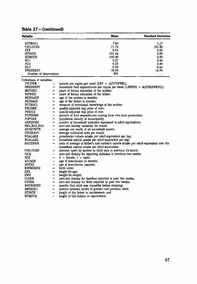
Tkble 27—(continued)

Variable Mean Standard Deviation

NUTRSC1CHILDCRESEXHTFATHHTMOTHRD1RD2RD3FFEXWKPC


7.8071.740.53

161.44150.40

0.270.250.24

30.56995

3.27103.00

0.505.896.950.440.440.43

16.76

Definitions of variables:YPCPWKFFEXWKPCM0THEDFATHEDMOTHAGEFATHAGENUTRSC1PRC0RNPRRICEPCTHOMEPOPDENADEQVHHRD1,RD2,RD3AVNETWTHCULTARPCPCALAE0HCALAEQRATI0PAR

CHILDCRESICKSEXACCAGEAGESQBRTHORDRZHAZWHDIARRFEVERMNTHBFEDBRTHSP1HTFATHHTMOTH

income per capita per week (LNY = ln[YPCPWK]);household food expenditures per capita per week (LNFFEX = ln[FFEXWKPC));years of formal education of the mother;years of formal education of the father;age of the mother in months;age of the father in months;measure of nutritional knowledge of the mother;quality-adjusted real price of corn;quality-adjusted real price of rice;percent of food expenditures coming from own-farm production;population density of municipality;number of household members expressed in adult-equivalents;zero-one dummy variables for round;average net worth of all household assets;average cultivated area per round;preschooler calorie intake per adult-equivalent per day;household calorie intake per adult-equivalent per day;ratio of average of father's and mother's calorie intake per adult-equivalent over thehousehold calorie intake per adult-equivalent;minutes spent by mother in child care in previous 24 hours;zero-one dummy for reporting sickness in previous two weeks;0 = female, 1 = male;age of preschooler in months;age of preschooler squared;birth order;height-for-age;weight-for-height;zero-one dummy for diarrhea reported in past two weeks;zero-one dummy for fever reported in past two weeks;months that child was breastfed before stopping;months between births of present and previous child;height of the father in centimeters; andheight of the mother in centimeters.

67

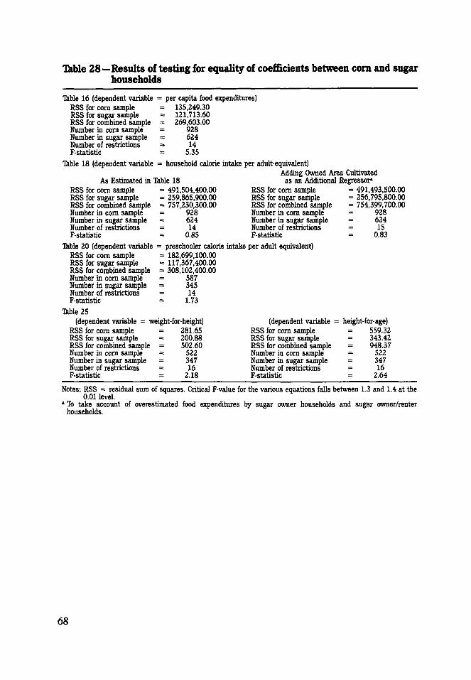
Table 28—Results of testing for equality of coefficients between corn and sugarhouseholds

Table 16 (dependent variable - per capita food expenditures)RSS for com sample = 135,249.30RSS for sugar sample = 121,713.60RSS for combined sample = 269,603.00Number in corn sample = 928Number in sugar sample = 624Number of restrictions = 14F-statistic = 5.35

Ikble 18 (dependent variable = household calorie intake per adult-equivalent)

As Estimated in Ikble 18RSS for com sample = 491,504,400.00RSS for sugar sample = 259,865,900.00RSS for combined sample = 757,230,300.00Number in com sample = 928Number in sugar sample = 624Number of restrictions = 14F-statistic = 0.85

Adding Owned Area Cultivatedas an Additional Regressor*

RSS for com sampleRSS for sugar sampleRSS for combined sampleNumber in com sampleNumber in sugar sampleNumber of restrictionsF-statistic

= 491,493,500.00= 256,795,800.00= 754,399,700.00

92862415

0.83

Table 20 (dependent variable = preschooler calorie intake per adult equivalent)RSS for com sample = 182,699,100.00RSS for sugar sample = 117,367,400.00RSS for combined sample = 308,102,400.00Number in com sample = 587Number in sugar sample = 345Number of restrictions = 14F-statistic = 1.73

Table 25(dependent variable = weight-for-height)

RSS for com sample = 281.65RSS for sugar sample = 200.88RSS for combined sample = 502.60Number in corn sample = 522Number in sugar sample = 347Number of restrictions = 16F-statistic = 2.18

(dependent variable = height-for-age)RSS for com sampleRSS for sugar sampleRSS for combined sampleNumber in com sampleNumber in sugar sampleNumber of restrictionsF-statistic

559.32343.42948.37

52234716

2.64

Notes: RSS = residual sum of squares. Critical F-value for the various equations falls between 1.3 and 1.4 at the0.01 level.

« To take account of overestimated food expenditures by sugar owner households and sugar owner/renterhouseholds.

68

Tkble 29—Results of Hausman tests for exogeneity of right-hand side variables

Table 16 (dependent variable

Sample HouseholdsAllAllAll

ComComComSugarSugarSugar

Table 18 (dependent variableCAOitA food exnenditMyllA JWV vAlfwUUXl

Sample HouseholdsAllAllAll

ComComComSugarSugarSugar

= per capita food expenditures; tested independent variable = per capita income)

Identifying Variable (s)CULTARPC, AVNETWTHCULTARPCAVNETWTHCULTARPC, AVNETWTHCULTARPCAVNETWTHCULTARPC, AVNETWTHCULTARPCAVNETWTH

= household calorie intake per adult-equivalent; testedures)

Identifying Variable (s)CULTARPC, AVNETWTHCULTARPCAVNETWTHCULTARPC, AVNETWTHCULTARPCAVNETWTHCULTARPC, AVNETWTHCULTARPCAVNETWTH

Estimated as Shownin Table 18

2.121.422.56

-0.53-0.62-0.16

2.371.882.47

t-Statistic for Fitted Value14.2212.6712.069.648.067.137.206.736.08

independent variable = per

Owned Area CultivatedAdded as Explanatory

Variable0.38

-0 .271.16

-0.55-0 .64-0 .11

0.680.251.01

Table 20 (dependent variable = preschooler calorie intake per adult-equivalent; tested independent variable =household calorie intake per adult-equivalent)

Sample Households Identifying Variable(s) t-Statistic for Fitted ValueAll FFEXWKPC 0.63

Corn FFEXWKPC -0 .14Sugar FFEXWKPC 1.07

Tested independent variable = ratio of parents' intake to household intakeAll FATHED 1.02

Corn FATHED 1.95Sugar FATHED -1.04

Tested independent variable = sickness of preschooler during past two weeksAll BRTHORDR -0.22

Corn BRTHORDR 0.22Sugar BRTHORDR 0.69

Table 25 (dependent variables = weight-for-height and height-for-age; tested independent variables = preschoolercalorie intake per adult-equivalent)

Identifying Dependent Variable Dependent VariableSample Households Variable (s) Is Weight-for-Height Is Height-for-Age

All FFEXWKPC -0 .16 2.17Corn FFEXWKPC 0.30 -0 .71Sugar FFEXWKPC -1 .11 2.93

Note: Critical t-value for the various equations falls between 1.96 and 1.98 at the 0.05 level for a two-tailed test.

69

BIBLIOGRAPHYBehrman, Jere, and Anil Deolalikar. 1988. Health and nutrition. In Handbook on economic

development, vol. 1, ed. H. B. Cheneiy and T. N. Srinavasan, 631-711. Amsterdam:North Holland Publishing Company

Bouis, Howarth E. 1989. Measuring the rate of technological change for rice productionin the Philippines: Implications for agricultural policy under economic recovery.International Food Policy Research Institute, Washington, D.C. Mimeo.

Bouis, Howarth E., and Lawrence J. Haddad. 1989. Estimating the relationship betweencalories and income: Does choice of survey variable matter? International FoodPolicy Research Institute, Washington, D.C. Mimeo.

Bouis, Howarth E., and Eileen Kennedy. 1989. Traditional cash crop schemes' effects onproduction, consumption, and nutrition: Sugarcane in the Philippines and Kenya.Paper presented at the IFPRI-INCAP workshop on "Commercialization of agricul-ture and household food security: Lessons for policies and programmes," 9-11March, Antigua, Guatemala.

Bouis, Howarth E., Kathleen DeWatt, Eileen Kennedy, Per Pinstrup-Andersen, IsabelNieves, and Joachim von Braun. 1984. A common framework for research on theincome and nutrition effects of increasing commercialization of semisubsistenceagriculture. International Food Policy Research Institute, Washington, D.C. Mimeo.

Braun, Joachim von, and Eileen Kennedy. 1986. Commercialization of subsistence agricul-ture: Income and nutritional effects in developing countries. Working paper on commer-cialization of agriculture and nutrition no. 1. Washington, D.C: International FoodPolicy Research Institute.

Braun, Joachim von, David Hotchkiss, and Maarten Immink. 1989. Nontraditional exportcrops in Guatemala: Effects on production, income, and nutrition. Research report 73.Washington, D.C: International Food Policy Research Institute.

Braun, Joachim von, Detlev Puetz, and Patrick Webb. 1989. Irrigation technology andcommercialization of rice in The Gambia: Effects on income and nutrition. Researchreport 75. Washington, D.C: International Food Policy Research Institute.

Braun, Joachim von, Hartwig de Haen, and Juergen Blanken. Forthcoming. Process and.effects of commercialization of African agriculture in a most densely populated area(Rwanda): Consequences for food security policy. Research report. Washington, D.C:International Food Policy Research Institute.

Corpus, Velona A., Antonio J. Ledesma, Azucena B. Limbo, and Howarth E. Bouis. 1987.The commercialization of agriculture in the southern Philippines: The income,consumption, and nutrition effects of a switch from corn to sugar production for tencase study households in Bukidnon (Phase I report for the Philippine Cash CroppingProject). International Food Policy Research Institute, Washington, D.C. Mimeo.

Dewey, Kathryn. 1980. The impact of agricultural development on child nutrition inTabasco, Mexico. Medical Anthropology 2 (1): 21.

Fleuret, Patrick, and Anne Fleuret. 1980. Nutrition, consumption, and agriculturalchange. Human Organization 39 (March): 250.

70

. Socioeconomic determinants of child nutrition in Taita, Kenya: A callfor discussion. Readers Forum: 8.

Food and Nutrition Research Institute. 1984. Second nationwide nutrition survey: Philip-pines, 1982. Manila: National Science and technology Authority.

Gross, Daniel, and Barbara A. Underwood. 1971. Technological change and caloriecosts: Sisal agriculture in northeastern Brazil. American Anthropologist 73 (March):725.

Haddad, Lawrence J. 1987. Agricultural household modelling with intrahousehold fooddistribution: A case study of commercialization in a southern Philippine province.Ph.D. dissertation, Stanford University, Stanford, Calif., U.S.A.

Haddad, Lawrence J., and Howarth E. Bouis. 1989. The impact of nutritional status onagricultural productivity: Wage evidence from the Philippines. International FoodPolicy Research Institute, Washington, D.C. Mimeo.

Hausman, J. A. 1978. Specification tests in econometrics. Econometrica 46 (November):1251-1271.

Hausman, Jerry A., and William E. Taylor. 1981. Panel data and unobservable individualeffects. Econometrica 49 (November): 1377-1398.

Hazell, Peter B.R., and Ailsa Roell. 1983. Rural growth linkages: Household expenditurepatterns in Malaysia and Nigeria. Research report 41. Washington, D.C: InternationalFood Policy Research Intitute.

Herdt, Robert. 1987. A retrospective view of technological and other cnanges inPhilippine rice farming, 1965-1982. Economic Development and Cultural Change 35Qanuary): 329-349.

Hernandez, Mercedes, C. P. Hidalgo et al. 1974. Effect of economic growth on nutritionin a typical community. Ecology of Food and Nutrition 4 (March): 283-291.

Hillman, Jimmye S. 1981. The role of export cropping in less developed countries.American Journal of Agricultural Economics 63 (2): 375.

Hsiao, Cheng. 1986. Analysis of panel data. New York: Cambridge University Press.

Johnston, Bruce, and Peter Kilby. 1975. Agriculture and structural transformation. NewYork: Oxford University Press.

Kennedy, Eileen T., and Bruce Cogill. 1987. Income and nutritional effects of thecommercialization of agriculture in southwestern Kenya. Research report 63. Washing-ton, D.C: International Food Policy Research Institute.

Lambert, J. N. 1978. Does cash cropping cause malnutrition? National Planning Office,Port Moresby, Papua New Guinea. Mimeo.

Lim, Antonio. 1987. Export crops in the Philippines with special emphasis on Mind-anao: A political economy study (Phase III report for the Philippine Cash CroppingProject). International Food Policy Research Institute, Washington, D.C. Mimeo.

Mellor, John. 1976. The new economics of growth. Ithaca, N.Y.: Cornell University Press.

71

National Economic and Development Authority. 1974.1971 census of agriculture. Manila:NEDA, National Census and Statistics Office.

1985.1980 census of agriculture. Manila: NEDA, National Census andStatistics Office.

Nelson, Gerald. 1988. Sugar in the Philippines: Policy responses to a distorted worldmarket. Food Policy 13 (August): 283-292.

Pitt, Mark M., and Mark R. Rosenzweig. 1985. Health and nutrient consumption acrossand within farm households. The Review of Economics and Statistics 67 (May):212-223.

Ranis, Gustav, and Frances Stewart. 1987. Rural linkages in the Philippines andTaiwan. In Macropolicies for appropriate technology in developing countries, ed. FrancesStewart, 140-191. Boulder, Colo., U.S.A.: Westview Press.

Rosegrant, M., L. Gonzales, H. Bouis, andj. Sison. 1987. Price andinvestment policies forfood crop sector growth in the Philippines. Report submitted to the Asian DevelopmentBank. Washington, D.C.: International Food Policy Research Institute.

Singh, Inderjit, Lyn Squire, and John Strauss. 1986. Agricultural household models:Extensions, applications, andpolicy. Baltimore, Md., U.S.A.: Johns Hopkins UniversityPress.

72

RECENT IFPRI RESEARCH REPORTS (continued)

61 THE PILOT FOOD PRICE SUBSIDY SCHEME IN THE PHILIPPINES: ITS IMPACT ON INCOME,FOOD CONSUMPTION, AND NUTRITIONAL STATUS, August 1987, by Marito Garcia and PerPinstrup-Andersen

60 POPULATION POLICY AND INDIVIDUAL CHOICE: A THEORETICAL INVESTIGATION, June1987, by Marc Nerlove, Assaf Razin, and Efraim Sadka

59 PRODUCTION INCENTIVES IN PHILIPPINE AGRICULTURE: EFFECTS OF TRADE AND EX-CHANGE RATE POLICIES, May 1987, by Romeo M. Bautista

58 THE FOOD STAMP SCHEME IN SRI LANKA: COSTS, BENEFITS, AND OPTIONS FOR MODIFI-CATION, March 1987, by Neville Edirisinghe

57 CEREAL FEED USE IN THE THIRD WORLD: PAST TRENDS AND PROJECTIONS TO 2000,December 1986, by J. S. Sarma

56 THE EFFECTS OF TRADE AND EXCHANGE RATE POLICIES ON AGRICULTURE IN ZAIRE,November 1986, by Tshikala B. Tshibaka

55 THE EFFECTS OF TRADE AND EXCHANGE RATE POLICIES ON AGRICULTURE IN NIGERIA,October 1986, by T. Ademola Oyejide

54 WEATHER AND GRAIN YIELDS IN THE SOVIET UNION, September 1986, by Padma Desai

53 REGIONAL COOPERATION TO IMPROVE FOOD SECURITY IN SOUTHERN AND EASTERNAFRICAN COUNTRIES, July 1986, by Ulrich Koester

52 FOOD IN THE THIRD WORLD: PAST TRENDS AND PROJECTIONS TO 2000, June 1986, byLeonardo A. Paulino

51 DETERMINANTS OF AGRICULTURAL POLICIES IN THE UNITED STATES AND THE EUROPEANCOMMUNITY, November 1985, by Michel Petit

50 GOVERNMENT EXPENDITURES ON AGRICULTURE AND AGRICULTURAL GROWTH IN LATINAMERICA, October 1985, by Victor J. Elfas

49 LIVESTOCK PRODUCTS IN THE THIRD WORLD: PAST TRENDS AND PROJECTIONS TO 1990AND 2000, April 1985, by J. S. Sarma and Patrick Yeung

48 RURAL HOUSEHOLD USE OF SERVICES: A STUDY OFMIRYALGUDA TALUKA, INDIA, March1985, by Sudhir Wanmali

47 EVOLVING FOOD GAPS IN THE MIDDLE EAST/NORTH AFRICA: PROSPECTS AND POLICYIMPLICATIONS, December 1984, by Nabil Khaldi

46 THE EFFECTS ON INCOME DISTRIBUTION AND NUTRITION OF ALTERNATIVE RICE PRICEPOLICIES IN THAILAND, November 1984, by Prasarn Trairatvorakul

45 THE EFFECTS OF THE EGYPTIAN FOOD RATION AND SUBSIDY SYSTEM ON INCOME DISTRI-BUTION AND CONSUMPTION, July 1984; by Harold Alderman and Joachim von Braun

44 CONSTRAINTS ON KENYA'SFOOD AND BEVERAGE EXPORTS, April 1984, by Michael Schluter

43 CLOSING THE CEREALS GAP WITH TRADE AND FOOD AID, January 1984, by Barbara Huddleston

42 THE EFFECTS OF FOOD PRICE AND SUBSIDY POLICIES ON EGYPTIAN AGRICULTURE,November 1983, by Joachim von Braun and Hartwig de Haen

41 RURAL GROWTH LINKAGES: HOUSEHOLD EXPENDITURE PATTERNS IN MALAYSIA ANDNIGERIA, September 1983, by Peter B. R. Hazell and Ailsa Roell

40 FOOD SUBSIDIES IN EGYPT: THEIR IMPACT ON FOREIGN EXCHANGE AND TRADE, August1983, by Grant M. Scobie

Howarth E. Bouis has been a research fellow at IFPRI since 1984.Lawrence J. Haddad, formerly a research analyst at IFPRI, is a lecturerin the Department of Economics at the University of Warwick, England.

RECENT IFPRI RESEARCH REPORTS

78 THE EFFECTS OF SUGARCANE PRODUCTION ON FOOD SECURITY, HEALTH, AND NUTRI-TION IN KENYA: A LONGITUDINAL ANALYSIS, December 1989, by Eileen Kennedy

77 THE DEMAND FOR PUBLIC STORAGE OF WHEAT IN PAKISTAN, December 1989, by Thomas C.Pinckney

76 AGRICULTURE AND ECONOMIC GROWTH IN ARGENTINA, 1913-84, November 1989, byYair Mundlak, Domingo Cavallo, and Roberto Domenech

75 IRRIGATION TECHNOLOGY AND COMMERCIALIZATION OF RICE IN THE GAMBIA: EFFECTSON INCOME AND NUTRITION, August 1989, by Joachim von Braun, Detlev Puetz, and PatrickWebb

74 FOOD PRODUCTION IN A LAND-SURPLUS, LABOR-SCARCE ECONOMY: THE ZAIRIAN BASIN,June 1989, by Tshikala B. Tshibaka

73 NONTRADITIONAL EXPORT CROPS IN GUATEMALA: EFFECTS ON PRODUCTION, INCOME,AND NUTRITION, May 1989, by Joachim von Braun, David Hotchkiss, and Maarten Immink

72 RICE PRICE FLUCTUATION AND AN APPROACH TO PRICE STABILIZATION IN BANGLADESH,February 1989, by Raisuddin Ahmed and Andrew Bernard

71 STORAGE, TRADE, AND PRICE POLICY UNDER PRODUCTION INSTABILITY: MAIZE INKENYA, December 1988, by Thomas C. Pinckney

70 AGRICULTURE IN THE GATT: AN ANALYSIS OF ALTERNATIVE APPROACHES TO REFORM,November 1988, by Joachim Zietz and Alberto Valdes

69 CONSEQUENCES OF DEFORESTATION FOR WOMEN'S TIME ALLOCATION, AGRICULTURALPRODUCTION, AND NUTRITION IN HILL AREAS OF NEPAL, October 1988, by Shubh K.Kumar and David Hotchkiss

68 COFFEE BOOM, GOVERNMENT EXPENDITURE, AND AGRICULTURAL PRICES: THE COLOM-BIAN EXPERIENCE, August 1988, by Jorge Garcia Garcia and Gabriel Montes Llamas

67 NATURE AND IMPACT OF THE GREEN REVOLUTION IN BANGLADESH, July 1988, by MahabubHossain

66 THE BRAZILIAN WHEAT POLICY: ITS COSTS, BENEFITS, AND EFFECTS ON FOOD CONSUMP-TION, May 1988, by Geraldo M. Calegar and G. Edward Schuh

65 CREDIT FOR ALLEVIATION OF RURAL POVERTY: THE GRAMEEN BANK IN BANGLADESH,February 1988, by Mahabub Hossain

64 COOPERATIVE DAIRY DEVELOPMENT IN KARNATAKA, INDIA: AN ASSESSMENT, December1987, by Harold Alderman

63 INCOME AND NUTRITIONAL EFFECTS OF THE COMMERCIALIZATION OF AGRICULTUREIN SOUTHWESTERN KENYA, November 1987, by Eileen T. Kennedy and Bruce Cogill

62 AGRICULTURAL RESEARCH IN NEPAL: RESOURCE ALLOCATION, STRUCTURE, AND INCEN-TIVES, September 1987, by Ram P. Yadav

(continued on inside back cover)

International Food Policy Research Institute1776 Massachusetts Avenue, N.W.Washington, D.C. 20036 USA

effects of agricultural commercialization on land tenure...

Documents