effects of a switchgrass buffer strip on soil
TRANSCRIPT
Florida International UniversityFIU Digital Commons
FIU Electronic Theses and Dissertations University Graduate School
11-13-2007
Effects of a switchgrass buffer strip on soilmicroorganisms near a field applied withendosulfanCristina Clark-CuadradoFlorida International University
DOI: 10.25148/etd.FI14060849Follow this and additional works at: https://digitalcommons.fiu.edu/etd
Part of the Environmental Sciences Commons, and the Environmental Studies Commons
This work is brought to you for free and open access by the University Graduate School at FIU Digital Commons. It has been accepted for inclusion inFIU Electronic Theses and Dissertations by an authorized administrator of FIU Digital Commons. For more information, please contact [email protected].
Recommended CitationClark-Cuadrado, Cristina, "Effects of a switchgrass buffer strip on soil microorganisms near a field applied with endosulfan" (2007).FIU Electronic Theses and Dissertations. 2379.https://digitalcommons.fiu.edu/etd/2379

FLORIDA INTERNATIONAL UNIVERSITY
Miami, Florida
EFFECTS OF A SWITCHGRASS BUFFER STRIP ON SOIL MICROORGANISMS
NEAR A FIELD APPLIED WITH ENDOSULF AN
A thesis submitted in partial fulfillment of the
requirements for the degree of
MASTER OF SCIENCE
m
ENVIRONMENTAL STUDIES
by
Cristina Clark-Cuadrado
2007

To: Interim Dean Mark Szuchman College of Arts and Sciences
This thesis, written by Cristina Clark-Cuadrado, and entitled Effects of a Switchgrass Buffer Strip on Soil Microorganisms near a Field Applied with Endosulfan, having been approved in respect to style and intellectual content, is referred to you tor judgment.
We have read this thesis and recommend that it be approved.
Kevin E. O'Shea
Stewart T. Reed
Krishnaswamy Jayachandran, Major Professor
Date of Defense: November 13, 2007
The thesis of Cristina Clark-Cuadrado is approved.
Interim Dean Mark Szuchman College of Arts and Sciences
Dean George Walker University Graduate School
Florida International University, 2007
ll

ACKNOWLEDGMENTS
I wish to thank the members of my committee for their assistance and advice in
accomplishing this project, Dr. Mahadev Bhat for his support and guidance throughout
my graduate career, and the USDA Subtropical Research Station for the space, time, and
equipment provided for my research. A special thanks to Mark Sullivan, for his
knowledge in pesticide application and help to create the test plots, and to Chris Dunn
and Ric Joseph for their never-ending help in the field and in the lab.
I also want to thank Dr. Paulette Johnson and Jennifer Reixach for their statistical
assistance~ Dr. Jennifer Richards for her help and knowledge in plant identification; Dr.
Kateel Shetty for his help in microbial analyses; and Michael and Kevin Clark-Cuadrado,
for their help with soil analyses.
A special acknowledgement to USDA/CSREES under the 2005 Hispanic Serving
Institute Higher Education Grants Program (Award# 2005-38422-15940) for funding my
research.
111
ABSTRACT OF THE THESIS
EFFECTS OF A SWITCHGRASS BUFFER STRIP ON SOIL MICROORGANISMS
NEAR A FIELD APPLIED WITH ENDOSULF AN
by
Cristina Clark-Cuadrado
Florida International University, 2007
Miami, Florida
Professor Krishnaswamy Jayachandran, Major Professor
A field study to detennine the effects of a switchgrass buffer strip (SBS) on soil
microorganisms near a field applied with endosulfan was carried out. Soil samples were
taken from a SBS and bare soil area downslope from a field applied with endosulfan at
different distances, days, and two seasons (wet and dry). Soil samples were analyzed for
endosulfan, soil fungi, and bacteria. Analysis of endosulfan concentrations was done by
reversed-phase liquid chromatography. No endosulfan runoff was detected by this
method. Analysis of soil fungi and bacteria was done by fungal and bacterial enumeration
by plate count method on rose bengal agar and tryptic soy agar, respectively.
Soil fungi and bacteria were higher in the SBS than in the bare soil area. Also, soil
bacteria was higher during the wet season than during the dry season. The opposite trend
was observed for soil fungi.
1V
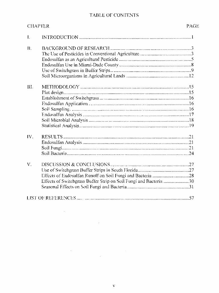
TABLE OF CONTENTS
CHAPTER PAGE
I. INTRODlJCTION ............................................................................................. 1
II. BACKGROUND OF RESEARCH ........... " ...................................................... 3 The Use of Pesticides in Conventional Agriculture ........................................... 3 Endosulfan as an Agricultural Pesticide ........................................................... 5 Endosulfan Use in Miami-Dade County ............................................................ 8 Use ofSwitchgrass in Buffer Strips ................................................................... 9 Soil Microorganisms in Agricultural Lands .................................................... 12
III. METI-IODOLOGY .......................................................................................... 15 Plot design ........................................................................................................ 15 Establishment of Switchgrass ......................................................................... 16 Endosulfan Application ... __ .............................................................................. 16 Soil Satnpling .................................................................................................. 16 Endosulfan Analysis ........................................................................................ 17 Soil Microbial Analysis ................................................................................... 18 Statistical }\nalysis ........................................................................................... 19
IV. RESULTS ........................................................................................................ 21 Endosulfan Analysis ........................................................................................ 21 Soil Fungi ......................................................................................................... 21 Soil Bacteria ..................................................................................................... 24
V. DISCUSSION & CONCLUSIO~S ................................................................. 27 Use of Switchgrass Buffer Strips in South Florida .......................................... 27 Effects of Endc,sulfan Runoff on Soil Fungi and Bacteria .............................. 28 Effects of Switchgrass Buflcr Strip on Soil Fungi and Bacteria .................... .30 Seasonal Effects on Soil Fungi and Bacteria ................................................... 3 l
LIST OF REFERENCES .................. , ......................................................................... 57
v

LIST OF TAI3LES
TABLE PAGE
l. Fungal count ANO\t"A table .................................................................................... 48
2. Fungal count during wet and dry seasons ............................................................... .48
3. Fungal count for bare soil and switchgrass buffer strip treatments ........................ .48
4. Fungal count for days 0, 1, and 28 .......................................................................... .49
5. Pairwise comparisons between seasons and plant covers for fungal count ............ .49
6. Fungal count by season and plant cover ................................................................. .49
7. Fungal counts for bare soil and switchgrass butTer strip treatments, distance, and days 0, 1, and 28 ............................................................... , ................ 50
8. Pairwise comparisons between treatments and distance for days 0, 1, and 28 for fungal counts ..................................... , ................................................... 51
9. Bacterial count ANOV A table ................................................................................. 52
10. Bacterial count during wet and dry seasons ........................................................... 52
11. Bacterial count for bare soil and switchgrass buffer strip treatments .................... 52
12. Bacterial count for days 0, 1, and 28 ..................................................................... 53
13. Pairwise comparisons between seasons and plant covers for bacterial counts ...... 53
14. Bacterial count by season and plant cover.. ........................................................... 53
15. Bacterial count for bare soil and switchgrass buffer strip treatments, distance, and days 0, 1, and 28 .......... " ................................................................... 54
16. Pairwise comparisons between treatments and distance for days 0, 1, and 28 for bacterial count ...................................... , ............................................... 55
17. Painvise comparisons between days and treatments for distances 0.3 and 0.9 m for fungal count ............................................................................................ 56
Vl

18. Painvise comparisons between days and treatments for distances 0.3 and 0. 9 m for bacterial count ..................... ,. ................................................................. 56
VII
LIST OF FIGURES
FIGURE PAGE
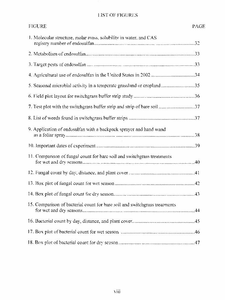
1. Molecular structure, molar ma::.s, s,)lubility in water, and CAS registry number of endosulfan ................................................................................. 32
2. Metabolism of endosulfan ........................................................................................ 33
3. Target pests of endo5ulfan ..................................................................................... .33
4. Agricultural use of endosulfan in the United States in 2002 ................................... 34
5. Sea:mnal microbial activity in a temperate grassland or cropland ........................... 35
6. Field plot layout for switchgrass buffer strip study ................................................. 36
7. Test plot with the switchgrass buffer strip and strip of bare soil ............................. 37
8. List of weeds found in switchgrass buffer strips .................................................... .37
9. Application of endosulfan with a backpack sprayer and hand wand as a foliar spray ....................................................................................................... 38
10. Important dates of experin1ent .......................... ,. ............... "' .................................. 39
11. Companson of fungal count for bare soil and switchgrass treatments for "''et and dry seasons .......................................................................................... 40
] 2. Fungal count by day, distance, and plant cover .................................................... .41
13. Box plot of fungal count for wet season ............................................................... .42
14. Box plot of fungal count for dry season ................................................................ .43
15. Comparison ofbacterial count for bare soil and switchgrass treatments for wet and dry seasons .......................................................................................... 44
16. Bacterial count by day, distance, and plant cover.. ............................................... .45
17. Box plot of bacterial count for wet season ........................................................... .46
18. Box plot of bact,;rial count fl.1r dry srason ........................................................... .4 7
Vlll

CHAPTER I
INTRODUCTION
Information on the effectiveness of buffer strips for the reduction of endosulfan
runoff from agricultural fields is limited. Though studies have been conducted in the
greenhouse (Mcrsie et al., 2005), field studies are needed to document the fate and
transport of endosulfan and its effects on soil biology. Modeling the fate and transport of
endosulfan through a vegetative buffer strip is needed to understand, predict, and prevent
endosulfan contamination of waterways, soils, and ecosystems. Furthermore, few studies
have evaluated the potential of switchgrass to reduce endosulfan pollution and improve
soil quality when used as a buffer strip.
Soil bacteria and fungi play a significant role in agricultural soils. Pathogenic soil
bacteria and fungi receive significant attention from farmers and soil conservationists due
to their negative effects on agricultural productivity. However. most soil bacteria and
fungi are beneficial to soil, plant, and the environment. Bacteria and fungi play vital roles
in agricultural soils and natural environments, such as their effect on organic matter
turnover and nutrient cycling (Wood, 1989). There is limited information on the effects
of endosulfan on soil bacteria and fungi. Information on the effects of endosulfan runoff
passing through a switchgrass filter strip can help agricultural landowners manage their
endosulfan applications and design of filter strips to prevent contamination of adjacent
natural areas. Furthermore, this information can give fam1ers insight on possible
secondary effects of endosulfan application on soil bacteria and fungi, helping them make
more educated decisions about managing soil quality.
The objectives of this study were to determine the effectiveness of a switchgrass
bufier strip in reducing endosulfan runoff and to study the effects of endosulfan on soil
microbial populations. Previous studies indicate that a switchgrass buffer strip will be
more successful in abating endosulfan runoff than a bare ground soil (Lee ct al., 1998).
However, butTer strips may also increase infiltration, thus causing problems for
groundwater (USDA, 2002). The effects of endosulfan on soil bacterial and fungal
populations were also studied, as well as the effects of a switchgrass buffer strip on soil
bacterial and fungal populations adjacent to a field applied with endosulfan. Higher
bacterial and fungal populations were expected in the soil of the switch grass buffer strip
than in the bare soil strip. In addition, bacteria and fungi will increase with the distance
from the point of endosulfan application.
2

CHAPTER II
BACKGROUND OF RESEARCH
The Use of Pesticides in Conventional Agriculture
Conventional agriculture has often been blamed for the overall decline of
ecosystem health. Since agricultural areas cannot be separated from the surrounding
ecosystems, natural resource management must include agricultural as well as natural
areas for healthier agroecosystems. Agricultural runofT frequently carries pesticides,
heavy metals, and nutrients that are hannful to beneficial insects and animals, as well as
endanger human health, fisheries, and tourism (UNEP, 1999). Some pesticides are lost to
the atmosphere through volatilization, however most applied pesticides remain in the soil
(Wright et al., 1993). Once in the environment, pesticides may be absorbed by plants and
other organisms, chemically decomposed, volatilized, adsorbed onto soil particles,
subjected to runoff: and leached through the soil profile (Rao et al. 2006). Urban
development and agricultural operations have decreased the amount of vegetated areas
along bodies of water able to absorb and stop or reduce the movement of pollutants
before reaching the water bodies.
Knowledge of the fate and transport of pesticides is essential in reducing off-site
movement of these contaminants. Although pesticides may enter the environment from
point sources (such as spills or improper disposal), nonpoint sources (such as agriculture)
are the main contributors of pesticides into natural environments (EPA, 1992). The main
properties of a pesticide affect its behavior after application are solubility, adhesion,
degradation, and persistence.
3
Solubility: Pesticides that are soluble in water are likely to leach through the soil
and contaminate groundwater. or flow with surface water and contaminate streams,
rivers, lakes, or other bodies of water. In general, water solubilities of pesticides higher
than 30 parts per million (ppm) have an increased tendency to leach down through the
soil profile (Landon eta!., 1994).
Adhesion: Pesticides often adhere to soil particles or organic matter through
adsorption. Pesticides that adhere to soil particles have a lower leaching potential than
water-soluble pesticides (Buttler et al., 2003). However, studies have shown that
pesticide molecules that tightly adhere to soil particles may not be easily broken down by
microorganisms (Landon et al. 1994) and may therefore persist longer in the
environment.
Degradation: Chemical reactions break down or degrade pesticides through time.
Break down may occur through microbial degradation, chemical degradation (by
chemical reactions not involving microorganisms), or photodegradation (light mediated
chemical reactions). Degradation of a pesticide does not signify that the pesticide is less
harmful. Often, the products of the degradation of pesticides are as or more harmful than
the original pesticide and may persist longer in the environment. For example, research
conducted by the United States Geological Survey (USGS) and Southern Illinois
University scientists indicates that the metabolites of the pesticides chlorpyrifos and
malathion are about 100 times more toxic than the parent compounds (Sparling et al.,
2007).
Persistence: Persistence describes a pesticide's continuing existence in the
environment. Persistence is measured by the amount of time it takes for half of the active
4

ingredient of the pesticide to degrade, otherwise known as its half-life. The half-life of a
pesticide is dependent on the nature of the chemical itself and several environmental
factors, such as soil type, temperature, light, moisture, microorganisms, etc. Persistent
pesticides, including endosulfan, are considered to last in the environment longer than 6
months (Moriarty, 1975).
Endosulfan as an Agricultural Pesticide
The chemical commonly called endosulfan was first used as a wood preservative;
however, it was registered as a pesticide in 1954 to control agricultural pests such as
aphids, spittlebugs, and whiteflies. Endosulfan is a restricted-use pesticide classified as a
chlorinated hydrocarbon insecticide and acaricide. Chlorinated hydrocarbons, in
particular organochlorine insecticides are considered to be persistent in the environment
(EPA, 2002) and have a high potential to bioaccumulate in organisms. Their persistence
and the fact that they require small amounts of applied chemical to achieve their goal
keeps application costs low. Some well-known organochlorine insecticides are DDT,
aldrin, dieldrin, heptachlor, chlordane, telodrin, difocol, and lindane (IUP AC, 1972).
Endosulfan, like most other organochlorine insecticides, is banned in several countries
due to its persistence in the environment and its toxicity to humans and animals (Kegley
et al., 2007). However, endosulfan is not banned in the United States and is widely used
for agricultural purposes.
Endosulfan has undergone the United States Environmental Protection Agency
(EPA) re-registration process several times with amendments to the label due to
environmental and human health concerns and lack of data on the effects and behavior of
endosulfan on several organisms (EPA, 2002). In 2000, residential use of endosulfan in
5

the United States was prohibited due to health concerns. The last re-registration of
endosulfan under the EPA was in 2002 (EPA, 2002). Earlier in 2007, the European
Commission proposed to include endosulfan in the list of Persitent Organic Pollutants
banned under the Stockholm Convention (PANNA, 2007).
The chemical name for endosulfan is 6,7,8,9, 1 0-hexachloro-1 ,5,5a,6,9,9a
hexahydro-6,9-methano-2,4,3-benzodioxathiepin-3-oxide, and its formula is
C9H6CL60 3S (Figure 1). Commercial endosulfan is composed of two isomers: 70 percent
a-endosulfan and 30 percent B-endosulfan, which have different properties (Kegley et al.,
2007). The a-isomer is more toxic, more volatile, and less water soluble than the P
isomer. However, the B-endosulfan isomer is more persistent in the environment than the
a-isomer (EPA, 2002). Both endosulfan isomers are metabolized initially to endosulfan
sulfate via oxidation and hydrolysis (Sutherland et al., 2000). Endosulfan sulfate is even
more persistent than the parent material (K won et al., 2005). Endosulfan sulfate then
metabolizes into endosulfan-dioL endosulfan hydroxyether, and endosulfan-lactonc.
These changes are shown in Figure 2. The toxicity of endosultan-sulfate to mammals is
about the same as for the parent compound itself, whereas the diol, the hydroxyether, and
the lactone can be considered nontoxic (IUPAC, 1972). These nontoxic metabolytes have
a lethal dose (LD50) ranging from I 50-15000 mg/kg in rats, whereas the toxic endosulfan
isomers have an LD50 of 18 to 160 mg/kg in rats (EXTOXNET, 1996). For the purpose of
this study, only toxic forms of endosulf~m will be of interest. The molecular structure,
molar mass, and solubility in water of the toxic forms of endosulfan can be found in
Figure 1. The half life of commercial endosulfan and its metabolite endosulfan-sulfate
ranges from 9 months to 6 years in soil (EPA, 2002). Endosulfan has a high affinity to
6

sorb to soil and is likely to be associated predominantly with suspended particles in
runoff (EPA, 2002).
Endosulfan is commonly sold commercially under the trade names Thiodan(RJ,
Phaser@, and Thionex@. Technical grade endosulfan is sold as 95 percent active
ingredient (a.i.). Endosulfan is also sold commercially as a 9 to 34 percent a.i.
emulsifiable concentrate, and a 1 to 50 percent a.i. wettable powder found in wettable
bags. It can be applied by groundboom sprayer, fixed-wing aircraft, chemigation, airblast
sprayer, rights of way sprayer, low and high pressure hand wand sprayer, backpack
sprayer, and dip treatment (EPA 2002). A 300- foot minimum spray drift buffer for
aerial applications between the treated crop and environmentally sensitive areas or
waterways is specified on the label.
Endosulfan is an endocrine disruptor and a neurotoxin that acts as a contact and
stomach poison to several agricultural pests (EPA 2002). Figure 3 includes a list of
endosulfan's target pests. It can be used on a wide variety ofvegetables, fruits, cereals,
ornamental shrubs, trees, vines, and herbaceous plants. Its main use in the United States
is on cotton, tomatoes, potatoes, apples, tobacco, pears, cucumbers, lettuce, green beans,
and squash (EPA, 2002). Endosulfan is a very persistent chemical that may stay in the
environment for lengthy periods particularly in acidic media (EPA, 2002).
Endosulfan has been found in areas that have never had endosulfan application,
such as the Arctic region and several National Parks. Endosulfan is problematic for fish,
amphibians, birds, and mammals. In fact, "Endosulfan was the most frequently detected
insecticide in tadpole and adult from tissues in a California study" (EPA, 2002). It has
been blamed for over 91 incidents of fish kills and damage to aquatic and semi-aquatic
7

organisms in the United States since I 97L mostly in California, South Carolina, and
Louisiana. About 32 percent of these incidents were directly attributable to runoff (EPA
2002). Endosulfan has also caused fish kills on five continents (EPA. 2002) and
deformations. abnormalities, and death in animals and humans due to its application ncar
them. Since endosulfan is highly toxic and has a high potential to bioaccumulatc in fish
and other animals, this problem is of great concern.
Endosulfan can be absorbed through the skin. In humans and mammals
endosulfim affects the nervous system. Symptoms include imbalance, difficulty
breathing, vomiting. convulsions, and loss of consciousness. The kidneys, liver, blood,
and parathyroid gland are the organs most likely to be affected (EXTOXNET, 1996).
Studies with cows, sheep, and pigs also show that endosulfan causes temporary blindness
(for about a month) (EXTOXNET. 1996). Animals should not be allowed to graze on
pasture that has been contaminated with cndosulfan. Applicators and handlers of
endosulfan, though, are at most risk and should be particularly careful with the pesticide.
Endosulfan Use in Miami-Dade County
Miami-Dade County is a major agricultural producer. It is the county in Florida
that has the second highest market value of agricultural products sold (NASS, 2004). The
use of chemicals for agricultural production in Miami-Dade can negatively impact the
soil, water, air and other natural resources of the area. In 2002, 10 million pounds of
agrochemicals were used and recorded (Hapeman et al., 2002). The climate in Miami
Dade, being warn1 most of the year, increases the amount of pests and weeds and the
spread of pathogens in agricultural operations. Therefore, the amount of chemicals
needed for high agricultural output is great. Heavy and frequent rainstorm events between
8
May and October cause pesticides and other agrochemicals to leach through or run off the
surface of treated fields. South Florida's expansive aquatic, amphibian, and avian fauna
(both permanent and migratory) are particularly at high risk to endosulfan poisoning.
Several agrochcmicals including endosulfan have already been found in South Florida's
canals, which drain into the Florida Bay, the Atlantic Ocean, and the Gulf of Mexico
(Harman Fetcho, 2005). Agrochemicals can also easily enter the Everglades National
Park due to its proximity to these agricultural lands. In Miami-Dade County, an annual
average of over 45.5 grams a.i. of endosulfan per square kilometer of agricultural land is
used, making Miami-Dade County one of the heaviest users of this pesticide in the
country (Figure 4). In Miami-Dade County, most of endosulfan use is due in part by the
continuous and heavy agricultural production of tomatoes, green beans, and squash.
Use of Switchgrass in Buffer Strips
Pesticides that bind to soil particles through adsorption, such as endosulfan, are
transported with soil particles suspended in runoff (Buttler et al., 2003). Deposition of
contaminated sediment in a body of water can lead to persistent environmental and health
problems since the pollutant could be released slowly as the sediment gets stirred in the
water. Vegetative filters, or buffer strips, are natural or manmade strips of herbaceous
vegetation between disturbed areas, such as cropland, and areas that are environmentally
sensitive, such as a river or a lake. Among other things, they are used to improve water
quality by reducing sediment runoff and transport of nutrients, animal wastes, and
pesticides from agricultural lands to water bodies.
It is very important to have a shallow sheet flow through the filter strip for it to
provide the benefits sought. Rills and gullies must be repaired immediately to prevent
9

areas of concentrated flow. The vegetation in buffer strips must also be mowed on a
regular basis to promote thick vegetation (USDA, 2002). Trapped sediment needs be
removed or redistributed as needed to prevent the formation of rills and gullies (USDA,
2002).
The conditions in vegetative filter strips, both biological and physical factors,
favor increased water infiltration and therefore the reduction of dissolved contaminants
carried in runoff (USDA, 2002). Studies indicate that water infiltration under buffers can
be as much as five times higher than in adjacent cultivated fields and pastures (USDA,
2002). T'his increase in soil infiltration is caused by several factors: The extensive root
system in filter strips increases biological activity by supplying an energy source to soil
organisms. These organisms, in tum, degrade pesticides and other contaminants. The
increased organic matter found in filter strips improves soil aggregation and slows down
runoff, reducing erosion of contaminated particles .
Vegetative fi Iter strips have other benefits aside from their potential reduction of
contaminants in runoff. They can serve as habitat and food for beneficial insects and
wildlife, or as a corridor between two natural areas of suitable habitat for many species,
increasing the animal's chances of finding food, water, shelter, and a suitable climate
(USDA, 2002).
Also, erosion control is another benefit of vegetative filter strips. Eroding banks
can remove land, reducing its size and become sediment in the water. Soil particles
suspended in the water damage aquatic habitat, degrade drinking water quality, and
reduce water holding capacity in wetlands, lakes, and reservoirs (Schultz, 1995). Eroding
10
banks are also dangerous to farmers. Filter strips can act as a natural barrier, keeping
equipment from rolling on steep ditches or riverbanks.
To avoid damage to the vegetative filter strip, it is best to use vegetation that is
resistant to the herbicides and other pesticides that will be applied upslope. Fescue is the
most commonly used grass for filter strips (Blanco-Canqui et al., 2005), although
canarygrass, and bermudagrass are also commonly used. Desirable grasses, though, will
vary with the location and specific purpose of the filter strip. Native, tall, erect, stiff
stemmed perennial grasses that produce dense vegetation and have extensive root
systems are preferred and work best for filter strips.
Switchgrass (Panicum virgatum L.), is a native wam1-season tall grass that
tolerates drought, very wet conditions, and soils low in nutrients. It produces high yields
with very low applications, if any, of fertilizer. Switchgrass also spreads through both
seeds and rhizomes, fonning a thick sod. It has recently received attention as a grass for
vegetative buffer strips and has proven to work better than other grasses in various
studies. Blanco-Canqui et al. (2005), for example, found that switchgrass planted along a
fescue vegetative buffer strip was more effective in reducing runoff than an only-fescue
buffer strip ofthe same width. Mersie et al. (2005) found that a 19-inch wide strip of
switchgrass reduced runoff from sediment coarser than 0.125 mm (fine sands and
coarser) by 90 percent. In addition, switchgrass is adapted to a variety of climates (from
wann, southern climates to colder, northern climates) and tolerant of triazine herbicides
that may be used upslope in the field. Its use can prove useful throughout most of the
United States.
11

Soil Microorganisms in Agricultural Lands
Attention needs to be given to soil microorganisms in agricultural lands since they
are an integral part in maintaining productive soils. Soil microorganisms decompose
organic compounds (including some pesticides), cycle nutrients making them available to
plants and other organisms, sequester carbon, suppress diseases malignant to agricultural
crops, and play an integral role in water dynamics by creating soil aggregates (Wood,
1989).
Bacteria and fungi are the smallest of soil microorganisms, with a cell width of
less than 1 )lm and 10 )lm, respectively (Wood, 1989). However, they are the most
abundant organisms in the majority of soils. On average, there are between 106 and 109
bacteria in a gram of soil (Wood, 1989), translating into about one ton of bacterial
biomass in an acre of soil. Fungi are also found in large quantities in the soil. In
agricultural lands, there can be several yards of fungi in one gram of soil, tens to
hundreds of yards in one gram of prairie soil, and one to forty miles in one gram of
coniferous forest soil (Tugel et al., 2000).
Both bacteria and fungi have similar roles: they break down residue and cycle
nutrients for plant use, produce compounds or have fungal hyphae that help create soil
aggregates, and protect plant roots from disease-causing organisms by competing with
them (Alexander, 1977). Since they are mostly aerobic, bacteria and fungi are present in
higher abundance in the top 10 em of the soil surface (Alexander, 1977) and most active
between Spring and Fall, after the last frost and before the first frost of the year (Tugel et
al., 2000). Figure 5 indicates seasonal bacterial and fungal activity in grasslands or
croplands. A study by Pietikainen eta!. (2005) also indicated that fungi and bacteria had
12
different temperature requirements: While fungal and bacterial growth rates had optimum
temperatures of around 25-30 °C, fungi was more adapted to lower temperatures and
bacteria was more adapted to higher temperatures. This temperature effect could have
implications for the warm Miami-Dade soils.
Fungi can live on the hard-to-metabolize organic material, such as woody debris.
They are more dominant in acidic soils, such as those found in woodlands. Under dry
conditions, fungi have an advantage over bacteria since they can use their hyphae to get
to the moisture pockets in the soil (Bardgett, 2005).
Bacteria are more numerous in areas where substrates that are easily metabolized
exist, for example in the rhizosphere and around young plant residue (Alexander, 1977).
They cannot move great distances and require moisture for reproduction and metabolism.
In very dry or in anaerobic conditions, such as when the soil floods or becomes
compacted, some bacteria can become dormant or die (Alexander, 1977). Highly acid or
alkaline conditions tend to inhibit many common bacteria (Wood, 1989). The optimum
pH for most species is near neutral. One of the most important features ofbacteria as a
group is their biochemical versatility. Some species of bacteria, like Pseudomonas 5p., is
able to metabolize a wide range of chemicals including pesticides. Thiobacillus
ferrooxidans gets its energy from the oxidation of reduced sulfur compounds and ferrous
ions (Wood, 1989). Several studies have successfully degraded endosulfan with the use
of bacteria. Sutherland et al. (2000), for example, used a Mycobacterium strain to degrade
technical endosulfan. Kwon et al. (2005) used Klebsiella pneumoniae to degrade
endosulfan without formation of the toxic metabolite, endosulfan sulfate. Kumar et al.
13

(2006) have been able to degrade endosulfan with the use of S'tenotrophomonas
maltophilia and Rhodococcus erythropolis.
14

CHAPTER III
METHODOLOGY
The procedures below were repeated twice: once during the wet season (June to
October) and again during the dry season (November to March). For the purpose of this
study, the wet season will be identified as WS and the dry season as DS.
Plot design
The plots are located in an open area at the USDA, Subtropical Horticulture
Research Station in Miami, FL containing a Pennsuco Marl (coarse-silty, carbonatic, .
hyperthermic typic fluvaquent) soil. A 10 x 15m section of land was cleared and graded
to provide a 3 to 5° slope. The slope was created to produce runoff and move soil
downslope (Figure 6). Several 3 m wide rows with 46 em row spacing of snap beans
were planted along a 11.2 m long by 2.4 m wide strip in the center, upslope section of the
field. Switchgrass buffer strips, alternating with strips of bare soil 1.8 m long by 2.8 m
wide, were planted downslope from the edge of the bean field. For WS, the switchgrass
was planted by direct seeding on the buffer strip areas. ForDS, the switchgrass was
grown in trays for 4-5 weeks and transplanted as sod. Soil was raked to provide a smooth
slope from the snap bean area to the buffer area. A sprinkler irrigation system was set up
and used twice a week (if no rain occurred) to provide 1.3 em of water per irrigation.
Figure 7 shows a picture of the test plot with the switchgrass buffer strip and strip of bare
soil. Beans received 72 kg ha- 1 10-10-10 solid fertilizer broadcasted after emergence.
Switchgrass received monthly applications of approximately 10 kg ha-1 liquid 10-10-10
as a foliar spray.
15
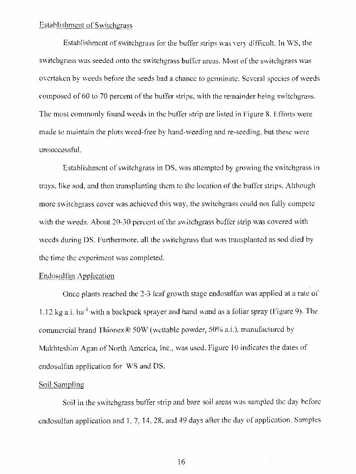
Establishment of Switchgrass
Establishment of switchgrass for the butTer strips was very difficult. In WS, the
switchgrass \vas seeded onto the switchgrass buffer areas. Most of the switchgrass was
ovettaken by weeds before the seeds had a chance to germinate. Several species of weeds
composed of 60 to 70 percent of the buffer strips, with the remainder being switchgrass.
The most commonly found weeds in the buffer strip are listed in Figure 8. EtTorts were
made to maintain the plots weed-free by hand-weeding and re-seeding, but these were
unsuccessful.
Establishment of switchgrass in DS, was attempted by growing the switchgrass in
trays, like sod, and then transplanting them to the location of the buffer strips. Although
more switchgrass cover was achieved this way, the switchgrass could not fully compete
with the weeds. About 20-30 percent of the switchgrass butTer strip was covered with
weeds during DS. Furthennore, all the switchgrass that was transplanted as sod died by
the time the experiment was completed.
Endosulfan Application
Once plants reached the 2-3 leaf growth stage endosulfan was applied at a rate of
1.12 kg a.i. ha-1 with a backpack sprayer and hand wand as a foliar spray (Figure 9). The
commercial brand Thionex® SOW (wettable powder, 50% a.i.), manufactured by
Makhteshim Agan of North America, Inc., was used. Figure 10 indicates the dates of
endosulfan application for WS and DS.
Soil Sampling
Soil in the switchgrass buffer strip and bare soil areas was sampled the day before
endosulfan application and 1, 7, 14, 28, and 49 days after the day of application. Samples
16

were taken at 0.3, 0.9, and 1.5 m from the edge of the bean field in both the switchgrass
buffer strip and bare soil areas. Soil samples, extracted with a 2 em diameter sampler to a
depth of 18 em, were divided between depths of 0-6 em (upper layer), 6-12 em (middle
layer), and 12-18 em (lower layer) from the soil surface. At each sampling date a
different row was randomly selected and sampled in the switchgrass buffer strip and in
the bare soil areas. Figure 10 indicates the days the soil was sampled for WS and DS. Soil
samples were stored in labeled sampling bags at 4 °C for no longer than two weeks
before analysis.
Endosulfan Analysis
Endosulfan was extracted from soil samples using the method described in
Siddique et al. (2003). Three grams each of air dried soil sample was shaken with 10 mL
of acetonitrile for 1 hour at 180 rpm on a New Brunswick Scientific Innova 2100
platform shaker. Solid particles were allowed to settle and the slmTy was centrifuged with
at 3400 rpm for l 0 minutes on a Fisher Scientific Marathon 8K bench-model centrifuge.
The supernatant was decanted, and the resulting mixture was stored in glass vials in the
dark at 4 oc for 5-6 weeks until analysis. Endosulfan was analyzed using reversed phase
high performance liquid chromatography (RP-HPLC) for a-endosulfan, ~-endosulfan,
and endosulfan sulfate. The mobile phase was acetonitrile:water (70:30 v/v) at a flow rate
of 1 mL min- 1• The injection volume was 20 J..!L. Standards for a-endosulfan, ~
endosulfan, and endosulfan sulfate were purchased from Chern Service, Inc. Retention
times were as follows: 8 min for endosulfan sulfate; 10.2 min for ~-endosulfan; and 11.4
min for a-endosulfan.
17
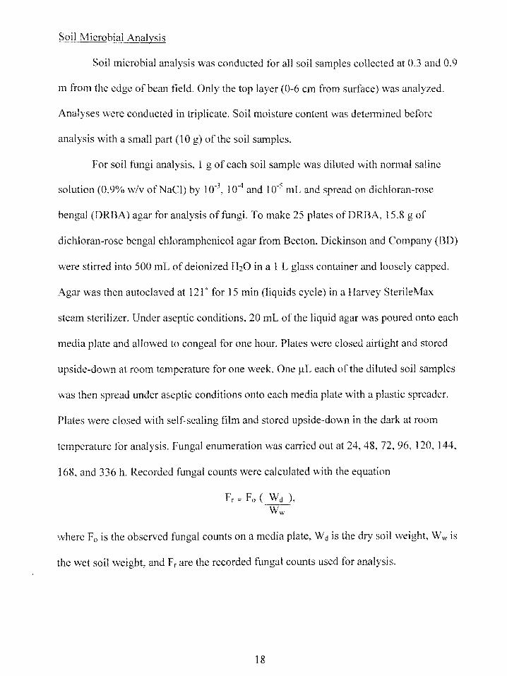
Soil Microbial Analysis
Soil microbial analysis was conducted for all soil samples collected at 0.3 and 0.9
m from the edge ofbean field. Only the top layer (0-6 em from surface) was analyzed.
Analyses were conducted in triplicate. Soil moisture content was detem1ined before
analysis with a small part (10 g) of the soil samples.
For soil fungi analysis, 1 g of each soil sample was diluted with normal saline
solution (0.9% w/v ofNaCl) by 10-3, 104 and 10-5 mL and spread on dichloran-rose
bengal (DRBA) agar for analysis offungi. To make 25 plates ofDRBA, 15.8 g of
dichloran-rose bengal chloramphenicol agar from Becton, Dickinson and Company (BD)
were stirred into 500 mL of deionized H20 in a 1 L glass container and loosely capped.
Agar was then autoclaved at 121° for 15 min (liquids cycle) in a Harvey SterileMax
steam sterilizer. Under aseptic conditions, 20 mL of the liquid agar was poured onto each
media plate and allowed to congeal for one hour. Plates were closed airtight and stored
upside-down at room temperature for one week. One 11L each of the diluted soil samples
was then spread under aseptic conditions onto each media plate with a plastic spreader.
Plates were closed with self-sealing film and stored upside-down in the dark at room
temperature for analysis. Fungal enumeration was carried out at 24, 48, 72, 96, 120, 144,
168, and 336 h. Recorded fungal counts were calculated with the equation
where F 0 is the observed fungal counts on a media plate, W d is the dry soil weight, W w is
the wet soil weight, and Fr are the recorded fungal counts used for analysis.
18

For soil bacteria analysis, 1 g of each soil sample was diluted with normal saline
solution (0.9% w/v ofNaCI) by 10-5, 10-6 and 10-7 mL and spread on tryptic soy agar
(TSA) with cycloheximide for analysis of bacterial colonies. To make 25 plates ofTSA,
1.5 g ofBD Bacto tryptic soy broth and 7.5 g ofBD Bacto agar were stirred with 500 mL
of deionized lbO and loosely capped. Agar was autoclaved at 121° for 15 min. (liquids
cycle). In a 10 mL beaker, 100 mg of Sigma cycloheximide was stirred with 7 mL of
deionized H20 until dissolved. Cycloheximide solution was filtered aseptically with a
200 nm filter into the agar container and stirred until evenly mixed. Under aseptic
conditions, 20 mL of the liquid agar was poured onto each media plate and allowed to
congeal for one hour. Plates were closed airtight and stored upside-down at room
temperature for one week. One f.J.L each of the diluted soil samples was then spread under
aseptic conditions onto each media plate with a plastic spreader. Plates were closed with
self-sealing film and stored upside-down in the dark at 28 oc for analysis. Bacterial
enumeration was carried out at 24, 48, 72, 96, 120, 144, 168, and 336 h. Recorded
bacterial counts were calculated with the equation
Br = Bo ( Wct ), Ww
where Bois the observed fungal counts on a media plate, W d is the dry soil weight, Ww is
the wet soil weight, and Br are the recorded fungal counts used for analysis.
Statistical Analysis
Statistically significant differences between fungal or bacterial populations in the
bare soil areas and switchgrass filter strips during the tested days, distances, and seasons
were determined post-experiment by an analysis of variance (ANOVA). The statistical
19

package SPSS (version 15) was used to calculate the one-way, two-way, and multivariate
ANOV As for all possible interactions between cover, season, day, and distance. Data
V•iere checked for normality prior to the ANOV A. Non-normal data were transformed
using the mathematical transformation square root (~x +.05) for fungi and bacteria and
rechecked for normality. Holm's sequential Bonferroni procedure was used for the three
way comparisons. Statistically significant differences between treatments were
determim:d at alpha (a)= 0.05.
20

Endosulfan Analysis
CHAPTER IV
RESULTS
RP-HPLC analysis of the soil samples did not yield the characteristic signals for
a, ~' and endosulfan sulfate. Endosulfan concentrations in the runoff from the bean field,
if any, must have been below the RP-IIPLC detection limit of 0.3 ppm. The solutions of
the extracted endosulfan from the soil samples have been saved and will be analyzed
post-experiment by gas chromatography with electron capture detector (ECD-GC), which
can detect endosulfan concentrations as low as 0.002 ppm. Samples analyzed by ECD
GC will examined for a-endosulfan, ~-endosulfan, and endosulfan sulfate.
Research performed by Joseph et al. (2007) on the same field plot as this research
was conducted indicates that there were no statistically significant differences observed
on soil respiration during the wet and dry seasons before and after endosulfan application.
During the wet season, C02 levels averaged at 335.8j.tmol mor1, soil moisture at 8.15
mbar, and soil temperature at 28.0 °C. During the dry season, C02 levels were 281.1
j.tmol mor1, soil moisture 7.7 mbar, and soil temperature 21.9 °C. The pH of all soil
samples was 7.8 ± 0.2.
Soil Fungi
As explained in the Methods section, soil samples were diluted to 1 o-3, 1 0-4 and
1 o-s mL before fungi analysis. Samples diluted to 1 o-3 mL had the most normal
population distribution. The soil in dilutions 10-4 and 1 o-s mL was too diluted for fungal
enumeration. Fungal counts for dilution 1 o-3 mL were mathematically transformed by
using their square root for further analysis of soil fungi. For discussion purposes, the
21

results presented here take into consideration this mathematical transformation and the
dilution factor.
The ANOV A revealed a significant individual effect by season, cover, and day.
The treatment interactions between season and cover; season and day; cover and day;
season, distance and day; cover, distance and day; and season, cover, distance and day
were also found to have a significant effect on soil fungi (p < 0.05) (Table 1).
Season comparison:
Overall mean fungal counts vvere significantly higher during DS than during WS
(p < 0.0001) (Table 2; Figure 11). During WS fungal counts had a mean of3.504 and a
95% confidence interval of2.764 and 4.243. During DS fungal counts had a mean of
8.787 and a 95% confidence interval of 8.047 and 9.526.
Cover comparison:
Overall mean fungal counts were also significantly higher in the switchgrass
buffer strip than in the bare soil areas (p < 0.0001) (Table 3; Figure 11). Fungal counts
had a mean of 7.606 with a 95% confidence interval of 6.867 and 8.346 for the
switchgrass buffer strip and a mean of 4.684 with a 95% confidence interval of 3.944 and
5.423 for the bare soil areas.
Day comparison:
Overall mean fungal counts also significantly increased through time (p <
0.0001 ). The fungal count mean for both seasons was 4.805 for day 0, 5.781 for day 1
and 7.850 for day 28, though variation exits (Table 4; Figure 12).
22
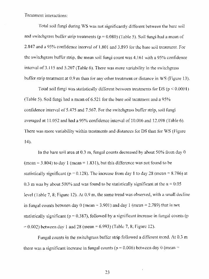
Treatment interactions:
Total soil fungi during WS was not significantly different between the bare soil
and switchgrass buffer strip treatments (p = 0.080) (Table 5). Soil fungi had a mean of
2.847 and a 95% confidence interval of 1.801 and 3.893 for the bare soil treatment For
the switchgrass buffer strip, the mean soil fungi count was 4.161 with a 95% confidence
interval of 3.115 and 5.207 (Table 6). There was more variability in the switchgrass
buffer strip treatment at 0.9 m than for any other treatment or distance in WS (Figure 13).
Total soil fungi was statistically different between treatments forDS (p < 0.0001)
(Table 5). Soil fungi had a mean of 6.521 for the bare soil treatment and a 95%
confidence interval of 5.475 and 7.567. For the switchgrass buffer strip, soil fungi
averaged at 11.052 and had a 95% confidence interval of 10.006 and 12.098 (Table 6).
There was more variability within treatments and distances for DS than for WS (Figure
14).
In the bare soil area at 0.3 m, fungal counts decreased by about 50% from day 0
(mean= 3.804) to day 1 (mean= 1.831 ), but this difference was not found to be
statistically significant (p = 0.128). The increase from day 1 to day 28 (mean= 8.786) at
0.3 m was by about 500% and was found to be statistically significant at the a = 0.05
level (Table 7, 8; Figure 12). At 0.9 m, the same trend was observed, with a small decline
in fungal counts between day 0 (mean= 3.901) and day 1 (mean= 2. 789) that is not
statistically significant (p = 0.387), followed by a significant increase in fungal counts (p
= 0.002) between day 1 and 28 (mean= 6.993) (Table 7, 8; Figure 12).
Fungal counts in the switchgrass buffer strip followed a different trend. At 0.3 m
there was a significant increase in fungal counts (p = 0.006) between day 0 (mean=
23

5.632) and day 1 (mean= 9.290), then a significant decrease (p = 0.002) between day 1
and day 28 (mean= 5.091). Fungal counts at day 0 and day 28 were not different (p =
0.673) (Table 7, 8: Figure 12). At 0.9 m fungal counts increased significantly (p = 0.012)
between day 0 (mean= 5.882) and day 1 (mean= 9.216), followed by a small increase
between day 1 and day 28 (mean= 1 0.528) that was not significant (p = 0.308) (Table 7,
8; Figure 12).
Soil Bacteria
Soil samples were diluted to 10-5, 10-6 and 10·7 mL before bacterial analysis.
Samples diluted to 1 o·6 mL had the most normal population distribution. The soil in
dilution 1 o·5 showed too many bacterial colonies for analysis and the soil in dilution 1 o·7
mL was too diluted to provide enough bacterial colonies for analysis. Bacterial counts for
dilution 1 o·6 mL were mathematically transformed by using their square root for further
analysis of soil bacteria. For discussion purposes, the results presented here take into
consideration this mathematical transformation and the dilution factor.
The soil bacteria ANOV A revealed a significant individual effect by season and
day. The treatment interactions between cover and distance; season and day; distance and
day; season, cover and distance; and season, distance and day were also found to have a
significant effect on soil fungi (p < 0.05) (Table 9).
Season comparison:
Overall mean bacterial counts were significantly higher in WS than in DS (p <
0.0001) (Table 1 0; Figure 15). During WS bacterial counts had a mean of 192.151 and a
95% confidence interval of 181.257 and 203.044. During DS bacterial counts had a mean
of 8.552 and a 95% confidence interval of -2.341 and 19.445 (Table 1 0).
24
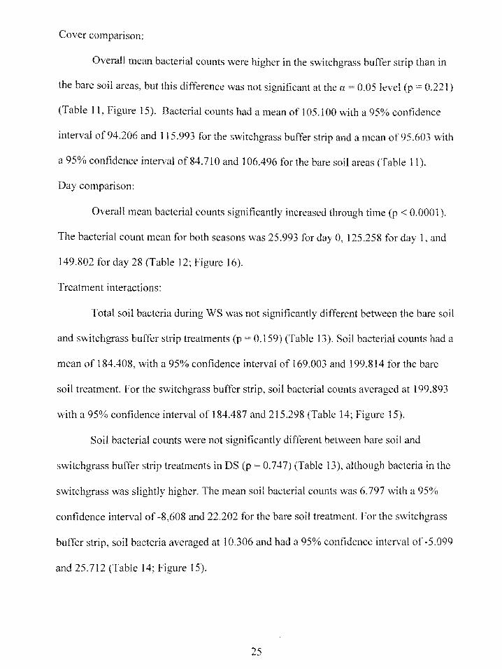
Cover comparison:
Overall mean bacterial counts were higher in the switchgrass buffer strip than in
the bare soil areas, but this difference was not significant at the a = 0.05 level (p = 0.221)
(Table 11, Figure 15). Bacterial counts had a mean of 105.100 with a 95% confidence
interval of94.206 and 115.993 for the switchgrass buffer strip and a mean of 95.603 with
a 95% confidence interval of 84.710 and 106.496 for the bare soil areas (Table 11 ).
Day comparison:
Overall mean bacterial counts significantly increased through time (p < 0.0001 ).
The bacterial count mean for both seasons was 25.993 for day 0, 125.258 for day 1, and
149.802 for day 28 (Table 1 2; Figure 16).
Treatment interactions:
Total soil bacteria during WS was not significantly ditrerent between the bare soil
and switchgrass buffer strip treatments (p 0.159) (Table 13). Soil bacterial counts had a
mean of 184.408, with a 95% confidence interval of 169.003 and 199.814 for the bare
soil treatment. For the switchgrass buffer strip, soil bacterial counts averaged at 199.893
with a 95% confidence interval of 184.487 and 215.298 (Table 14; Figure 15).
Soil bacterial counts were not significantly different between bare soil and
switchgrass buffer strip treatments in DS (p = 0.747) (Table 13), although bacteria in the
switchgrass was slightly higher. The mean soil bacterial counts was 6. 797 with a 95%
confidence interval of -8,608 and 22.202 for the bare soil treatment. For the switchgrass
buffer strip, soil bacteria averaged at 10.306 and had a 95% confidence interval of -5.099
and 25.712 (Table 14; Figure 15).
25

Bacteria increased steadily in the bare soil area from day 0 to day l to day 28 at
the 0.3 m distance. On day 0 mean bacterial counts were 52.846. By day 1 mean bacterial
count was 79.783, which was not significantly different at the a= 0.05 level (p = 0.158).
The increase in bacterial counts between day 1 and day 28 was significant (p < 0.0001),
averaging at 180.508 (Table 15, 16; Figure 16). At 0.9 m a different trend was observed:
there was a significant increase (p < 0.0001) in bacterial counts between day 0 (mean=
4.309) and day 1 (mean= 135.685). A small decrease in bacteria occurred by day 28,
where the mean was 53.016. This decrease was not significant at the a= 0.05 level (p =
0.034) (Table 15, 16; Figure 16).
Bacterial populations in the switchgrass buffer strip followed a similar trend to
that found in the bare soil area. At 0.3 m bacteria significantly increased from day 0
(mean= 43.288) to day 1 (mean 84.846) (p = 0.032). Another significant increase
occurred by day 28 (mean 163.782) (p < 0.0001) (Table 15, 16; Figure 16). At 0.9 m
bacterial counts also increased significantly between day 0 (mean= 3.528) and day 1
(mean= 200.720) (p < 0.0001 ). However, there was a significant decline in bacterial
counts by day 28 (mean= 134.433) (p = 0.001) (Table 15, 16; Figure 16).
26
CHAPTER V
DISCUSSION & CONCLUSIONS
Use of S witchgrass Bufier Strips in South Florida
Switchgrass is native to South Florida and a suggested species for buffer strips by
the USDA (USDA, 1999). However, this experiment showed the complexities of
switchgrass as the main vegetation in a buffer strip to reduce pesticide runoff due to the
problems in establishment and maintenance. Other studies have had success in reducing
contaminants using a switchgrass buffer strip (Blanco-Canqui et al., 2005; Mersie et al..
2005). The literature also indicates that Panicum virgatum is a hardy grass that tolerates
drought, very wet conditions. poor soils, and can be weedy or invasive in certain
circumstances (USDA, 2001 ). However, the unexpected hardships in establishing
switchgrass faced during this study indicate otherwise. The poor establishment of the
grass and high maintenance required to prevent weeds from overtaking the switchgrass
buffer strip and keeping it alive makes it inefficient for use in buffer strips in practical
scenarios.
The difficulty in establishing the switchgrass might have been due to the tillage
practice to the buffer strip area prior to switchgrass establishment. The seeds of weeds
that were there prior to the experiment could have germinated when exposed to sunlight
and taken over before the switchgrass seeds were able to germinate. Whether this is true
or not, farmers and landowners do not want to spend their resources in establishing buffer
strips that create complexities. Installation of buffer strips often does not benefit the
landowners themselves, but the surrounding land, water, and environment. Herbaceous
plants used for butTer strips should be easy to establish, very low maintenance, and
27
overall inexpensive to retain. They should also perform the task required, namely
preventing sediment, pesticide, and nutrient runoff.
An assessment of the location of the buffer strip should be done prior to
establishing a grass for this purpose. Local grasses that efTectively reduce runoff and
remain in the designated area throughout the year should be used first. Although there
was natural switch grass adjacent to the test plot for part of the year, the grass ''moved'' as
the weather changed and was eventually replaced by other grasses and broad leaf plants.
The switchgrass ncar the test field seemed to prefer shaded areas, where weed
competition is at a minimum. Farmers and landowners know their property best and have
seen the succession throughout the years and weather events. They should work closely
with experts to determine which grasses are best for them to use in butTer strips.
Effects of Endosulfan Runoff on Soil Fungi and Bacteria
Research performed by Joseph et al. (2007) on the same field plot as this research
was conducted indicates that there were no statistically significant differences observed
on soil respiration rates before and after endosulfan application. Soil respiration normally
refers to the total outflow of C02 at the soil surface. It is the combination of biotic,
chemical and physical processes. This is an indication that microbial respiration, a biotic
process, was not affected by the application of endosulfan.
The RP-HPLC endosulfan analysis did not provide any positive results because of
the lower detection limit of 0.3 ppm, therefore, the specific effects of endosulfan on soil
fungi and bacteria cannot be detem1ined. ECD-GC analysis of endosulfan concentrations
in the soil is required to accurately measure lower concentrations of endosulfan in the soil
28

not detected by the RP-HPLC. The ECD-GC can detect endosulfan concentrations as low
as 0.002 ppm to determine the effects of endosulfan on soil fungi and bacteria.
It can be assumed that the runoff from the bean field did not contain amounts of
endosulfan high enough to be deadly to most insects and higher animals at the 1.12 kg a.i.
ha-1 application rate per the toxicity estimates provided in the EPA's ECOTOXicology
database (EPA, 2007). Endosulfan concentrations causing mortality to bird species
(LD5o) are above 690 ppm except for the Northern bobwhite (Colinus virginianus) and
the Mallard duck (Anas platyrhynchos), whose LD50 are 42 and 28 ppm respectively
(EPA, 2007). The LD50 of most insects, except for a few that are targeted by endosulfan,
are also well above the 0.3 ppm detection limit of the RP-HPLC. No reptiles have an
LDso of 0.3 ppm or less (EPA, 2007). However, an LD50 of 0.3 ppm or below is common
in amphibians, some worms, crustaceans, and fish (Kegley, 2007). Endosulfan
concentrations below 0.3 ppm might not cause death in most species; however, they can
affect important neurological processes in several species causing imbalance, confusion,
difficulty breathing, convulsions, temporary blindness, loss of consciousness, and even
deformations.
It is important to note that endosulfan is toxic to humans, animals, and insects.
The results of our studies are not meant to replace or contradict the warnings and
suggestions made by the EPA and other toxicity studies, or provided on the endosulfan
pesticide label. This study imitated two yearly applications of endosulfan on a small field.
The accumulation of endosulfan runoff could and probably would be greater along
steeper sloping farmland, in larger fields, in fannland that is adjacent other fannland
29

using endosulfan. and in land that has had cndosulfan application for extended periods of
time.
EtTects of Switchgrass Buffer Strip on Soil Fungi and Bacteria
Switchgrass had a positive effect on soil fungi and bacteria. The mean fungal
counts for all seasons, distances, and days for the bare soil areas was 4.684. For the
switchgrass buffer strip, it was 7.606 (Table 3). The mean bacterial count for the bare soil
areas was 95.603. For the switchgrass buffer strip, it was 105.100 (Table 11 ).
According to the Soil Biology Primer (Tugel et al., 2000) and other sources
(Alexander, 1977; Wood, 1989; Bardgett, 2005) bacteria are more competitive when
substrates that are easy to metabolize are present. This includes fresh, young plant residue
and the compounds found near living roots. Bacteria are especially concentrated in the
rhizosphcre, where plants produce certain types of root exudates to encourage the growth
of protective bacteria. Fungal growth is also promoted with plant residue. The
switchgrass in the bufTer strip and the exudates from its extensive root system encouraged
growth of bacteria and fungi. The bare soil areas lacked this factor and therefore
supported less bacteria and fungi.
The results from this study indicate that buffer strips increase soil bacteria and
fungi and may be able to filter harmful bacteria from agricultural fields befc)re reaching a
body ofwater (Staddon et al., 2001; Boyer, 2006). As previously described, fungi and
especially bacteria can metabolize a wide range of chemicals including pesticides (Wood,
1989). Buffer strips can therefore decrease pesticide runoff by preventing the sediment to
which pesticide adsorbs and by metabolizing the pesticides that reach it. Since bacteria
30
and fungi also cycle nutrients, fertilizer runoff can also be reduced by these soil
organisms in the buffer strip.
Seasonal Effects on Soil Fungi and Bacteria
There was a significant difference in soil fungi and bacteria between the wet
season and the dry season. Soil fungi more than doubled from the wet season to the dry
season. The mean fungal count during the wet season was 3.504. During the dry season,
it was 8.787 (Table 2). Season had an opposite effect for soil bacteria. During the wet
season, the mean bacterial count was 115.688. During the dry season, it dropped to
15.777 (Table 10).
These results support the literature stating that, in drier conditions, soil bacteria
die or go dom1ant and soil fungi has an advantage since they can use their hyphae to get
to the moisture pockets in the soil (Bardgett, 2005). During the wet season, bacteria
dominated in the soil. During the dry season, fungi dominated in the soil and bacterial
numbers plummeted. The difference in soil fungi between the wet and dry seasons is not
as great as the difference in soil bacteria because fungi also flourish in wet conditions.
31

Common name techni cal endosulfan alpha ( o:) endosulfan beta ( ~) endosulfan endosul fan sulfate
Empirical formula CgH5CI60 3S CgH6CI60 3S CgH6CI50 3S C9H5CI6S04 01 01
~Qtr ~ ~ 01)- Cl
S Cl .
Molecular structure I . a a ~ /.o Cl ~ 01__1-; 0
Cl O - S 0 a o-&" II Cl
I a c1 0 o-s~o
0
CAS registry number 115-29-7 959-98-8 33213-65-9 1031-07-8
Molecular weiqht 406 .95 406 .93 406 .93 422 .90
Solubility in water'" 60 to 1 00 11g/L 530 ~g/L 280 1-lg/L 117 to 220 ~g/L
.. at 25 oc

Figure 2: Metabolism of endosulfan. From Ballschmitter et al., 1967.
H2 I c-o, s-o
I c-o I H2
Endosulfan I I I
""" H2 I
crxc:o c I H2
Endosulfan ether
H2 I
CC(~)s-o c-o I H2
Endosulfan sulphate
H CH '.. /
Endosulfan lactone
(1y c/"o \!A ~ further metabolites
c I H2
Endosulfan hydroxyether
----7 further metabolites
Endosulfan diol
Figure 3: Target pests of endosulfan, adapted from EPA (2002).
Target Pests:
Meadow spittlebug, Army cutworm, Aphids, Bean leaf skeletonizer, Cowpea curculio, Cucumber beetle, Flea beetle, Green stink bug,
Leafhoppers, Mexican bean beetles, Cabbage looper, Cabbage worm,
Cabbage aphid, Cucumber beetles, Whitefly, Cutworms, Thrips, Diamondback moth, Corn earworm, Boll weevil, Bollworm, Lygus bugs, Melonworm, Pickleworm, Rindworm, Squash beetle, Squash bug,
Blister beetle, Potato beetle, Rose chafer, Pepper maggot, Cinch bug, Crown mite, June bug, Harlequin bug, Grape phylloxera, and Grape leafhopper.
33

Figure 4: Agricultural use of endosulfan in the United States in 2002 created by the US Dept. of the Interior (2002).
Aver~e annual use of act1ve ingredient
ENDOSULFAN - insecticide 2002 estimated annual agricultural use
(pounds per square mile of agricultural land in county)
0 no estimated use
D o.oo1 to o.oo5 • 0.006 to 0.018 0 0.019 to 0.064
D o.oss to o.259
• >=0.26
Crops
cotton tomatoes potatoes apples tobacco pears cucumbers and pickles lettuce green beans squash
34
Total pounds applied
160060 88607 87452 62973 58016 43730 34370 33267 28923 28632
Percent national use
20.32 11.25 11.10
7.99 7.36 5.55 4.36 4.22 3.67 3.63

Figure 5: Seasonal microbial activity in a temperate grassland or cropland, created by Tugel et al.(2000).
Seasonal Microbial Activity
last frost
\
early summer
\
Month
35
late

'Tj cr'Q' s= """ (1>
Plot design 0\
2.8 m 'Tj (D'
downslope 0:: 1.5 m
'0 1.5m 0 ......
0.9 m 0.9 m ~ '<
0.3 m 0
0 .3 m s= ...... 8' """ Vl
~ . ...... (') ::;-
(10
E """ (")
upslope 3-5• slope llJ Vl Vl
w r:r 0\
s= ~ (1>
""" Vl ...... """
0.3 m 0 .3 m -o· Vl ...... s=
0.9 m 0.9 m 0.. '-<
1.5 m 1.5 m
downslope
11.2 m
Swithgrass buffer
. Bare soi l area
+ Sampling point
I Row of snap beans
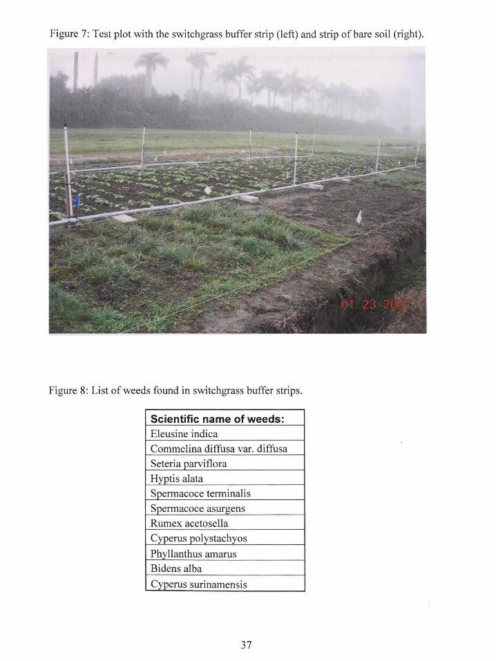
Figure 7: Test plot with the switchgrass buffer strip (left) and strip of bare soil (right).
Figure 8: List of weeds found in switchgrass buffer strips.
Scientific name of weeds: Eleusine indica
Commelina diffusa var. diffusa
Seteria parviflora
Hyrtis alata Spermacoce terminalis
Spermacoce asurgens
Rumex acetosella
Cyperus polystachyos
Phyllanthus amarus Bidens alba
Cyperus surinamensis
37
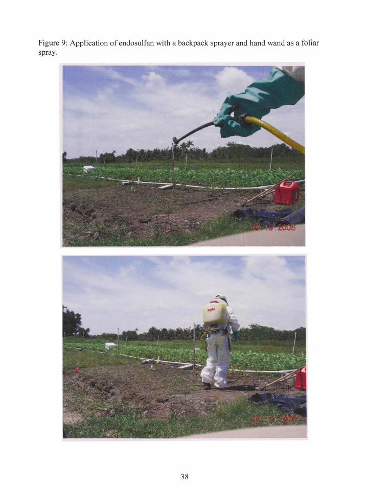
Figure 9: Application of endosulfan with a backpack sprayer and hand wand as a foliar spray.
-
38

Figure 10: Important dates of experiment.
Wet Dry Season (Summer to Fall 2006) (Winter to Spring 20071
Planting of switchgrass June 7th, 2006 November 15th, 2006
Planting of beans August 17th, 2006 December 20th, 2006
Endosulfan application September 13th, 2006 January 25th, 2007
Day 0 September 13th, 2006 January 25th, 2007 Cl
Day 1 c: September 14th, 2006 January 26th , 2007 c.. E Day 7 September 20th , 2006 February 1st, 2007
"' en Day 14 September 27th, 2006 February 8th, 2007 ·c;
Day 28 October 11th, 2006 February22nd, 2007 en Day49 November 11th, 2006 March 14th, 2007
Removal of bean plants October 18th, 2006 March 13th, 2007
39
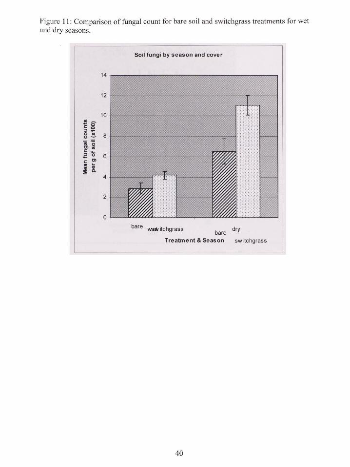
Figure 11: Comparison of fungal count for bare soil and switchgrass treatments for wet and dry seasons.
Soil fungi by season and cover
14
12
10 ~~~-... 0 c: 0 ::J ..... 0 )( 8 u-
bare W9!JN itchgrass bare dry
Treatment & Season sw itchgrass
40

Figure 12: Fungal count by day, distance, and plant cover.
14
12
0 0 ..... )( = 10 0 VI -0 C) 8 ... Qj a. VI -c: :::1 6 0 u iii C) c: :::1 4 -c: ns Qj
:!: 2
0
0 Application of endosulfan Day
28
41
121 Bare soil strip; 0.3 m
!ZI Bare soil strip; 0.9 m
o Switchgrass strip; 0.3 m
D Switchgrass strip; 0.9 m

Figure 13: Box plot of fungal count for wet season.
12.00
10.00
til- 8 .00 -o C:o :::::s.,... 0 >< o-n;=
6.00 C)o c: 1/)
:::::s-- 0 c: c:
"' ... (I) (I)
:! c. 4.00
2.00
0.00
bare
Cover
42
switchgrass
Distance
00.3 m ~ 0.9m

Figure 14: Box plot of fungal count for dry season.
20.00
15.00 ... Cl)
c.. Ill-.... 0 Co ::I-0 )( o---ns ·-C)o 10.00 c: Ill
~0 c: c ns Cl)
:::!:
5.00
0.00
bare
Cover
43
switchgrass
Distance
0 0.3 m ~ 0 . 9 m

Figure 15: Comparison of bacterial count for bare soil and switchgrass treatments for wet and dry seasons.
Ill~ .... o c: 0 ::JC!. 00 () .....
)( nl ~ ·c:: = Q) 0 ..... Ill ()
~~~-..0 0 c: C)
nl ... Q) Q)
::! Q.
Soil bacteria by season and cover
250T---------------------------------------~
200
150
100
50
o~~~tl81 __ ~~~£ZITl_J bare sw itchgrass sw itchgrass
wet
Treatment & Season
44
dry
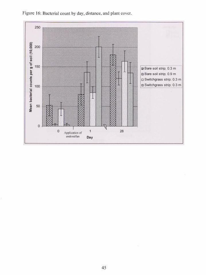
Figure 16: Bacterial count by day, distance, and plant cover.
0 0 0 c:i ~
0 t/) -0 Cl ... Ql Q.
J!l r::: ::J 0 ()
iii ·;: Ql -() Ill
..0
r::: Ill Ql
:::liE
200
150
100
50
0 Application of endosul fan Day
28
45
1'.01! Bare soil strip; 0.3 m
fZl Bare soil strip; 0.9 m
o Switchgrass strip; 0.3 m
III Switchgrass strip; 0.3 m
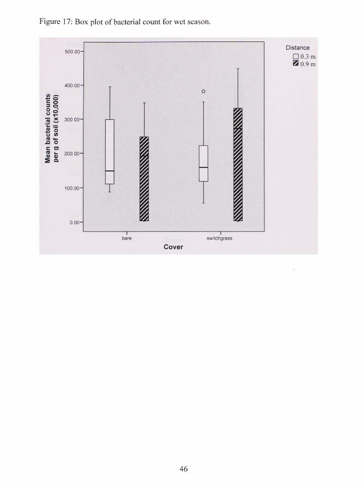
Figure 17: Box plot of bacterial count for wet season.
500.00 Distance
00.3 m ~0.9m
400.00 0
til--o co ::so 0 ~ (.)0 ..... - >< "'- 300.00 "i:-(1)"-_o (.) til ns-.c 0 c Cl nl ... 200.00 Q) Q)
:! c.
100.00
0.00
bare switchgrass
Cover
46

Figure 18: Box plot of bacterial count for dry season.
20.00
15.00 Ill-... 0 co :lO 0 -()0 ..... - >< "'-"i:-(I) ·-... o 1000 () Ill
"'-.c 0 c C)
"' ... (I) (I)
:::!: Q.
5.00
0.00
bare switchgrass
Cover
47
Distance
0 0.3 m ~ 0 .9m

Table 1: Fungal count ANOV A table.
Source df Type Ill SS Mean F Value Sig. Square
Season 1 502.384 502.384 103.132 < 0001 Cover 1 153.74 153.74 31.561 <.0001 Distance 1 11.879 11.879 2.439 0.125 Day 2 116.018 58009 11.908 < 0001 Season * Cover 1 46.578 46.578 9.562 0.003 Season * Distance 1 2.735 2.735 0.562 0.457 Cover * Distance 1 20.163 20.163 4.139 0.047 Season * Cover* Distance 1 4.504 4.504 0.925 0.341 Season* Day 2 117.719 58.86 12.083 <.0001 Cover* Day 2 157.308 78.654 16.146 <0001 Season * Cover * Day 2 6.512 3.256 0.668 0.517 Distance * Day 2 9.383 4.691 0.963 0.389 Season * Distance * Day 2 119.574 59.787 12.273 <.0001 Cover * Distance * Day 2 59.886 29.943 6.147 0.004 Season * Cover * Distance * Day 2 176.901 88.451 18.158 < 0001
Table 2: Fungal count during wet and dry seasons.
Season Mean Std. Error 95% Confidence Interval
Lower Bound Upper Bound
wet 3.504 .368 2.764 4.243 dry 8.787 .368 8047 9.526
Table 3: Fungal count for bare soil and switchgrass buffer strip treatments.
95% Confidence Interval Cover Mean Std. Error
Lower Bound Upper Bound
bare 4.684 .368 3.944 5.423 switchQrass 7.606 .368 6.867 8.346
48

Table 4: Fungal count for days 0, 1, and 28.
95% Confidence Interval Day Mean Std. Error
Lower Bound Upper Bound
0 4.805 .451 3.899 5.711 1 5.781 .451 4.875 6.687
28 7.850 .451 6.944 8.755
Table 5: Pairwise comparisons between seasons and plant covers for fungal count.
Season (I) Cover (J) Cover Mean
Std. Difference Sig.(a)
(1-J) Error
wet bare switchqrass -1.314 .736 .080 switchgrass bare 1.314 .736 .080
dry bare switchgrass -4.531 (*) .736 .000 switchgrass bare 4.531(*) .736 .000
Based on est1mated margmal means * The mean difference is significant at the .05 level. a Adjustment for multiple comparisons: Least Significant Difference (equivalent to no adjustments).
Table 6: Fungal count by season and plant cover.
Std. 95% Confidence Interval Season Cover Mean
Error Lower Bound Upper Bound
wet bare 2.847 .520 1.801 3.893 switch grass 4.161 .520 3.115 5.207
dry bare 6.521 .520 5.475 7.567 switchgrass 11.052 .520 10 006 12.098
49
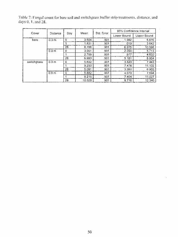
Table 7: Fungal count for bare soil and switchgrass buffer strip treatments, distance, and days 0. 1, and 28.
Cover Std. Error 95% Confidence Interval
Distance Day Mean Lower Bound Upper Bound
bare 0.3m 0 3.804 .901 1.992 5.616 1 1.831 .901 .019 3.642 28 8.786 .901 6.975 10.598
0.9 m 0 3.901 .901 2.090 5.713 1 2.789 .901 .977 4.600 28 6.993 .901 5.181 8.804
switchgrass 0.3m 0 5.632 .901 3.820 7.443 1 9.290 .901 7.478 11.102 28 5.091 .901 3.280 6.903
0.9m 0 5.882 .901 4.070 7.694 1 9.216 .901 7.404 11.027 28 10.528 .901 8.716 12.340
50
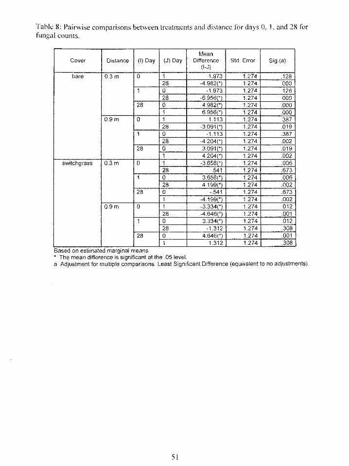
Table 8: Pairwise comparisons between treatments and distance for days 0, 1, and 28 for fungal counts.
Mean Cover Distance (I) Day (J) Day Difference Std. Error Sig.(a)
(1-J)
bare 0.3m 0 1 1.973 1.274 .128 28 -4 982(*) 1.274 .000
1 0 -1.973 1.274 .128 28 -6 956(*) 1.274 .000
28 0 4.982(*) 1.274 .000 1 6.956(*) 1.274 .000
0.9m 0 1 1.113 1.274 .387 28 -3.091 (*) 1.274 .019
1 0 -1.113 1.274 .387 28 -4.204(*) 1.274 .002
28 0 3 091(*) 1.274 .019 1 4.204(*) 1.274 .002
switch grass 0.3m 0 1 -3 658(*) 1.274 .006 28 .541 1.274 .673
1 0 3.658(*) 1.274 .006 28 4 199(*) 1.274 .002
28 0 -.541 1.274 .673 1 -4.199(*) 1.274 .002
0.9m 0 1 -3.334(*) 1.274 .012 28 -4.646(*) 1.274 .001
1 0 3.334(*) 1.274 .012 28 -1.312 1.274 .308
28 0 4 646(*) 1.274 .001 1 1.312 1.274 .308
Based on estimated margmal means * The mean difference is significant at the .051evel. a Adjustment for multiple comparisons: Least Significant Difference (equivalent to no adjustments).
51
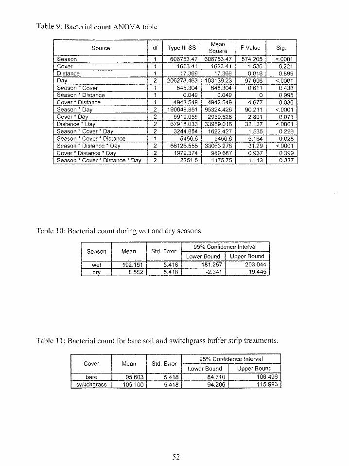
Table 9: Bacterial count ANOV A table
Source df Type Ill SS Mean
F Value Sig. Square
Season 1 606753.47 606753.47 574.205 <.0001 Cover 1 162341 1623.41 1.536 0.221 Distance 1 17.369 17.369 0.016 0.899 Day 2 206278.463 103139.23 97.606 <.0001 Season* Cover 1 645.304 645.304 0.611 0.438 Season * Distance 1 0.049 0.049 0 0.995 Cover • Distance 1 4942.549 4942.549 4.677 0.036 Season* Day 2 190648.851 95324.426 90.211 <.0001 Cover • Day 2 5919.055 2959.528 2.801 0.071 Distance * Day 2 67918.033 33959.016 32.137 <.0001 Season • Cover • Day 2 3244.854 1622.427 1.535 0.226 Season * Cover * Distance 1 5456.6 5456.6 5.164 0.028 Season * Distance * Day 2 66126.555 33063.278 31.29 <.0001 Cover * Distance * Day 2 1979.374 989.687 0.937 0.399 Season * Cover • Distance * Day 2 2351.5 1175.75 1.113 0.337
Table 1 0: Bacterial count during wet and dry seasons.
95% Confidence Interval Season Mean Std. Error
Lower Bound Upper Bound
wet 192.151 5.418 181.257 203.044 dry 8.552 5.418 -2.341 19.445
Table 11: Bacterial count for bare soil and switchgrass buffer strip treatments.
95% Confidence Interval Cover Mean Std. Error
Lower Bound Upper Bound
bare 95.603 5.418 84.710 106.496 switch grass 105.100 5.418 94.206 115.993
52

Table 12: Bacterial count for days 0, 1, and 28.
95% Confidence Interval Day Mean Std. Error
Lower Bound Upper Bound
0 25.993 6.635 12.651 39.334 1 125.258 6.635 111.917 138.600
28 149.802 6.635 136.461 163.144
Table 13: Pairwise comparisons between seasons and plant covers for bacterial counts.
Season (I) Cover (J) Cover Mean
Difference Std. Error Sig.(a) (1-J)
wet bare switch grass -15.484 10.836 .159 switch grass bare 15.484 10.836 .159
dry bare switchgrass -3.509 10.836 .747 switch grass bare 3.509 10.836 .747
Based on est1mated margmal means * The mean difference is significant at the .05 level. a Adjustment for multiple comparisons: Least Significant Difference (equivalent to no adjustments).
Table 14: Bacterial count by season and plant cover.
Season Cover Mean Std. Error 95% Confidence Interval
Lower Bound Upper Bound wet bare 184.408 7.662 169 003 199.814
switchgrass 199.893 7.662 184487 215.298 dry bare 6.797 7.662 -8.608 22.202
switchgrass 10.306 7.662 -5.099 25.712
53

Table 15: Bacterial count for bare soil and switchgrass buffer strip treatments, distance, and days 0, 1, and 28.
Cover Distance Day Mean Std. Error 95% Confidence Interval
LowerBound I UpperBound
bare 0.3m 0 52.846 13.271 26.163 79.529 1 79.783 13.271 53.101 106.466 28 180.508 13.271 153.825 207.191
0.9m 0 4.309 13.271 -22.374 30.991 1 135.685 13.271 109.002 162.367 28 120.486 13.271 93.803 147.168
switch grass 0.3m 0 43.288 13.271 16.605 69.971 1 84.846 13.271 58.163 111.529 28 163.782 13.271 137.099 190.465
0.9m 0 3.528 13.271 -23.154 30.211 1 200.720 13.271 174.037 227.402 28 134.433 13.271 107.750 161.116
54

Table 16: Pairwise comparisons between treatments and distance for days 0, 1, and 28 for bacterial count.
Mean Cover Distance (I) Day (J) Day Difference Std. Error Sig.(a)
(1-J)
bare 0.3m 0 1 -26.937 18.768 .158 28 -127 662(*) 18.768 .000
1 0 26.937 18.768 .158 28 -100 725(*) 18.768 .000
28 0 127.662(*) 18.768 .000 1 100.725(*) 18.768 .000
0.9m 0 1 -131.376(*) 18.768 .000 28 -116.177(*) 18.768 .000
1 0 131.376(*) 18.768 .000 28 15.199 18.768 .422
28 0 116.177(*) 18.768 .000 1 -15.199 18.768 .422
switchgrass 0.3m 0 1 -41 558(*) 18.768 .032 28 -120.494(*) 18.768 .000
1 0 41 558(*) 18.768 .032 28 -78.936(*) 18.768 .000
28 0 120.494(*) 18.768 .000 1 78 936(*) 18.768 .000
0.9m 0 1 -197.191(*) 18.768 .000 28 -130.904(*) 18.768 .000
1 0 197.191 (*) 18.768 .000 28 66.287(*) 18.768 .001
28 0 130.904(*) 18.768 .000 1 -66.287(*) 18.768 .001
Based on est1mated margmal means * The mean difference is significant at the .05 level. a Adjustment for multiple comparisons: Least Significant Difference (equivalent to no adjustments).
55

Table 17: Pairwise comparisons between days and treatments for distances 0.3 and 0.9 m for fungal count.
Mean Day Cover (I) Distance (J) Distance Difference Std. Error Sig.(a)
(1-J) 0 bare 0.3m 0.9m -.097 1.274 .939
0.9m 0.3m .097 1.274 .939 switch grass 0.3m 0.9m -.250 1.274 .845
0.9m 0.3m .250 1.274 .845 1 bare 0.3m 0.9m -.958 1.274 .456
0.9m 0.3m .958 1.274 .456 switchgrass 0.3m 0.9m .075 1.274 .954
0.9m 0.3m -.075 1.274 .954 28 bare 0.3m 0.9m 1.793 1.274 .166
0.9m 0.3m -1.793 1.274 .166 switchgrass 0.3m 0.9m -5.437(*) 1.274 .000
0.9m 0.3m 5.437(*) 1.274 .000 Based on est1mated margmal means * The mean difference is significant at the .05 level. a Adjustment for multiple comparisons: Least Significant Difference (equivalent to no adjustments).
Table 18: Pairwise comparisons between days and treatments for distances 0.3 m and 0.9 m for bacterial count.
Mean Day Cover (I) Distance (J) Distance Difference Std. Error Sig.(a)
(1-J) 0 bare 0.3 m 0.9m 48.538(*) 18.768 .013
0.9 m 0.3m -48.538(*) 18.768 .013 switchgrass 0.3m 0.9m 39.760(*) 18.768 .039
0.9m 0.3m -39.760(*) 18.768 .039 1 bare 0.3m 0.9m -55.901{*1 18.768 .005
0.9m 0.3m 55 901C2_ 18.768 .005 switch grass 0.3m 0.9 m -115.87 4(*) 18.768 .000
0.9m 0.3m 115.874(*) 18.768 .000 28 bare 0.3m 0.9m 60.022(*) 18.768 .002
0.9m 0.3m -60.022(*1 18.768 .002 switchgrass 0.3m 0.9m 29.349 18.768 .124
0.9m 0.3m -29.349 18.768 .124 Based on est1mated margmal means * The mean difference is significant at the .05 level. a Adjustment for multiple comparisons: Least Significant Difference (equivalent to no adjustments).
56

LIST OF REFERENCES
Agency for Toxic Substances and Disease Registry (ATSDR). Toxicological Prc!filefbr Endosulfan, update; US Department of Health and Human Services, 2000.
Alexander, Martin. Introduction to Soil Microbiology. 2nd ed.; John Wiley & Sons: New York, 1977; pp 16-35.
Ballschmitter, K.; Schophan, 1.; Tolg, G. The metabolization of endosu(fan in insects and mammals. Paper presented to the VI International Plant Protection Congress, Vienna, 1967.
Bardgett, Richard. The Biology ofSoil: A Community and Ecosystem Approach; Oxford University Press: New York, 2005; pp 24-56.
Blanco-Canqui, H.; Gantzer, C. J.; Anderson, S. H.; Alberts, E. E.; Thompson, A. L. Grass barrier and vegetative filter strip effectiveness in reducing runoff. sediment, nitrogen, and phosphoms loss. Soil Science Society ofAmerica Journal. 2005, 68, 1670-1678.
Boyer, A. Reducing Bacteria with Best Management Practices. Delaware Department of Natural Resources and Environmental ControL Watershed Assessment Section, 2006. Accessed online August 2006 at http://W\\'W.wr.udel.edu/ChristinaTribTeam/Fact%20Sheets/ReducingBacteria_w BMPs.pdf
Buttler, T.; Martinkovic, W.; Nesheim, O.N. Factors Influencing Pesticide 1\1ovement to Ground Water. Florida Cooperative Extension Service, Institute of Food and Agricultural Sciences, University of Florida, 2003.
Extension Toxicology Network (EXTOXNET). Pesticide Jnji.Jrmation Pro_files: Endosu(fan. A Pesticide Information Project of Cooperative Extension Offices of Cornell University, Oregon State University, the University ofldaho, and the University of California at Davis and the Institute for Environmental Toxicology, Michigan State University, 1996. Accessed online May 2006 at http://extoxnet.orst.edu/pips/endosulf.htm
Hapeman, C.J.; Rice, C.; McConnel, L.L.; Schmidt, W. Atmospheric Processes of Agricultural Pollutants That Affect Air and Water Quality: 2002 Annual Report. ARS Pro_ject, Environmental Management and Byproduct Utilization Laboratory. 2002. Project No. 1265-12220-003-00.
Harman Fetcho, J.A; Mcconnell, L.L.; Potter, T.L.; Rice, C.; Sadeghi, A.M.; Sefton, K.A.; Schaffer, B.A.; Curry, R.W.; Bialek Kalinski, K.M.; Smith, R.D.; Hapeman, C.J. Pesticide occurrence in selected South Florida canals and Biscayne
57

Bay during high agricultural activity. Journal of Agriculture and Food Chemistly. 2005,53 (15), 6040-6048.
International IUPAC Congress ofPesticide Chemistry, 2d, Tel-Aviv, 1971; }ate of Pesticides in Environment; Proceedings; Tahori, A. S., Ed.; Gordon and Breach: New York, 1972; pp 283-292.
Joseph, R.; Reed, S.; Clark-Cuadrado, C; Jayachandran, K. Effects of endosulfan on soil respiration. Presented at ASA-CSSA-SSSA Annual Meetings, New Orleans, LA, November 4-8, 2007; 448.
Kegley, S.; Hill, B.; Om1e, S. PAN Pesticide Database, Pesticide Action Network, North America: San Francisco, CA., 2007. Accessible online at http://www.pesticideinfo.org.
Kumar K.; Devi, S.S.; Krishnamurthi, K.; Kanade, G.S.; Chakrabarti, T. Enrichment and isolation of endosulfan degrading and detoxifying bacteria. Chemosphere. 2006, 68 (2), 317-322.
Kwon, G-S.; Sohn H-Y.;Shin, K-S.; Kim, E.; Seo, B-I. Biodegradation ofthe organochlorine insecticide, endosulfan, and the toxic metabolite, endosulfan sulfate, by Klebsiella oxytoca KE-8. Applied A1icrobiology and Biotechnolo;.,ry'. 2005, 67 (6), 845-850.
Landon, M.; Jacobsen, J.; Johnson, G. Pesticide Managementfor Water Quality Protection; Montana State University Extension Service, 1994.
Lee, K-H.; Isenhart, T.M.; Schultz, R.C.; Mickelson. S.K. Nutrient and sediment removal by switchgrass and cool-season grass filter strips in Central Iowa, USA. Agroforestry S'_vstems. 1998, 44 (2, 3), 121-132.
Mersie, W.; Seybold, C. A.; and McNamee, C.; Lawson, M.A. Comparison of switchgrass and tall fescue filter strips for abating endosulfan runoff moving at two different flow rates. Agriculture, Ecosystems, and Environment, 2005, under review.
Moriarty, F. Ed. Organochlorine Insecticides: Persistent Organic Pollutants; Academic Press: New York, 1975; pp 1-15.
Pesticide Action Network of North America (PANNA). Summary of the Proposalfor listing Endosuljcm in the Stockholm Convention on Persistent Organic Pollutants, 2007. Accessed online August 2007 at http://www.panna.org/resources/documents/endosulfanProposa!Stockholm.pdf
58
Pietikainen, J.; Pettersson, M.; Baath, E. Comparison of temperature effects on soil respiration and bacterial and fungal grovvth rates. Federation of European Microbiological Societies (FEMS) Microbiology Ecology. 2005, 52 (1), 49-58.
Rao, P.S.C.; Mansell, R.; Baldwin, L.B.; Laurent, M.F. Pesticides and their behavior in soil and water; Florida Cooperative Extension Service, Institute of Food and Agricultural Sciences; University of Florida, 2006.
Schultz, R.C.; Isenhart, T.M.; Colletti, J.P. Riparian Buffer Systems in Crop and Rangelands. Agroforestry and Sustainable Systems: Symposium Proceedings. USDA Forest Service General Technical Report RM-GTR-261, 1995. pp 13-27.
Siddique, T.; Zahir, Z.A.; Frankenberger, W.T. Reversed-Phase Liquid Chromatographic Method for Analysis of Endosulfan and Its Major Metabolites. Journal of Liquid Chromatography & Related Technologies. 2003,26 (7), 1069-1082.
Soil and Plant Analysis CounciL Soil analysis handbook of reference methods. CRC Press, Washington, DC, 1999.
Sparling, D.W.; Fellers, G. Comparative toxicity of chlorpyrifos, diazinon, malathion and their oxon derivatives to larval Rana boylii. Environmental Pollution. 2007, 147 (3), 535-539.
Staddon, W. J.; Locke M.A.; Zablotowicz, R. M. Microbiological Characteristics of a Vegetative Buffer Strip Soil and Degradation and Sorption of Metolachlor. Soil Science Society of America Journal. 2001, 65, 1136-1142.
Sutherland, T.D.; Home, I.; Lacey, MJ.; Harcourt, R.L.; Russell, R.J.; Oakeshott, J.G. Enrichment of an Endosulfan-Degrading Mixed Bacterial Culture. Applied and Environmental Microbiology. 2000, 66 (7), 2822-2828.
Tugel, A.; Lewandowski, A.; Happe-vonArb, D. Soil Biology Primer, Rev. Ed. Ankeny. Soil and Water Conservation Society, lowa, 2000.
U.N. Environmental Program (UNEP). Global Environmental Outlook 2000. Earthscan Publications: London, 2000.
U.S. Department of Agriculture (USDA). Plant Material Fact Sheet .. Natural Resources Conservation Service, Plant Material Programs. 1999. Accessed online May 2006 at http://plant-materials.nrcs.usda.gov/pubs/txpmsbrbffstrp332.pdf
U.S. Department of Agriculture (USDA). Plant Fact Sheet: Switchgrass. Natural Resources Conservation Service. 2001. Accessed online May 2006 at http://vvww.plants.usda.gov/factsheet/pdf/fs_pavi2.pdf
U.S. Department of Agriculture (USDA). Conservation Buffers to Reduce Pesticide Losses. Natural Resources Conservation Service (NRCS): Washington DC, 2002.
59
U.S. Department of Agriculture, National Agricultural Statistics Service (NASS). 2002 Census of Agriculture. Florida County Level Data. Accessed online on May 2006 at http://Vv~-Vw.agcensus.usda.gov.
U.S. Department of the Interior. Endosulfan Insecticide 2002 Estimated Annual Agricultural Use. National Water Quality Assessment Program Pesticide National Synthesis Project, 2002. Accessed online October 2006 at http://ca.water.usgs.gov/pnsp/pesticide _use_ maps/
U.S. Environmental Protection Agency (EPA). National Water Quality Inventory: 1990 Report to Congress. Office of Water, EPA, 503/9-92/006, August 1992.
U.S. Environmental Protection Agency (EPA). Reregistration eligibility decision for endosulfan. Office ofPrevention, Pesticides and Toxic Substances (OPPTS) EPA 738-R-02-013, 2002. Accessed online August 2006 at http:/ /Vvwvv.epa.gov/oppsrrd 1/REDs/endosul fan _red.pdf.
U.S. Environmental Protection Agency (EPA). 2007. ECOTOX User Guide: ECOTOXicology Database System. Version 4.0. A vail able online at: http:/www.epa.gov/ecotox/ search for endosulfan.
Wood, Martin. Soil Biology. Chapman and Hall: New York, 1989; pp 7-24.
Wright, R.J.; Witkowski, J.F.; Schulze, L.D. Water Resource Management: Water Quality. NebGuide. Institute of Agriculture and Natural resources. University of Nebraska, 1993.
60