effective use of monte carlo methods for simulating photon
TRANSCRIPT

Institutionen för medicin och vård Avdelningen för radiofysik
Hälsouniversitetet
Effective use of Monte Carlo methods for simulating photon transport with special reference to slab penetration
problems in X-ray diagnostics
Gudrun Alm Carlsson
Department of Medicine and Care Radio Physics
Faculty of Health Sciences

Series: Report / Institutionen för radiologi, Universitetet i Linköping; 49 ISSN: 0348-7679 ISRN: LIU-RAD-R-049 Publishing year: 1981 © The Author(s)
1981-10-19 ISSN 0348-7679
Effective use of Monte Carlo methods for simulating photon transport with special reference to slab penetration problems in X-raydiagnostics.
Gudrun Alm Carlsson
Avd för radiofysikUniversitetet i Linköping
REPORTULi-RAD-R-049
Effective use of Monte Carlo methods for simulating photon transport with special reference to slab penetration problems
by Gudrun Alm Carlsson
CONTENTS
Introduction . . . . . • . . . . • • • • . . • • . . . . . • • • . . . . . . • . . . • . . . . • . • . • . • • •• p 1
r. Basic considerations underlying the application of Monte Carlomethods to photon transport problems p 2
A. Presentation of a particular problem and conceivable so-lutions . . . . . . . . . . . . . . . . . . . . . . . . . . . . . . . . . . . . . . . . . . . . . . . .. P 2
B. Definitions of different field quantities ............... p 5
C. The concept of arandom walk and its mathematical descrip-tian . . . . . . . . . . . . . . . . . . . . . . . . . . . . . . . . . . . . . . . . . . . . . . . . . .. P 9
D. Transition probabilities" collision densities and rela-tions between collision densities and field quantities .. , p 11
1. Transition probabilities in an infinite homogeneousmedium and construction of transition probabilitydensities from physical interaction cross sections .... P 11
2. Collision densities • • • • • • • • • • • • • • • • • • • • • • • • • • • • • • • • .• P 2 O
Collision densities in an infinite homogeneous medium P 20
Collision densities in a finite homogeneous medium P 23
3. Relations between collision densities and fieldquantities P 25
E. The random selection of a value for a stochastic variable. p 30
1. Discrete stochastic variables ...............•........ p 31
2. Continuous stochastic variables .........•............ p 32
The distribution function method • • • • . . . • . • • • • • . . . • • • . • . .. p ;3 2
The rej ection method .............................•...... P 3 '+
Modification of the rejection method P 37
II. The generation of random walks and their use in estimatingfield quantities " p 39
A. Analogue simulation P 39

1. On the generation of random walks p 39
Re~ations between the coordinates in the system of the interacting photon and those of a fixed coordinate system .. p 43
2. The use of random walks in estimating field quantities ... p 47
The direct simulation estimator P 4 7
The last event estimator ................................• P 54
The absorption estimator P 56
The collisiori density estimator P 5 8
3. Comparison between estimates - efficiency and precisionof an estimate ......................•................... P 6l
The efficiency of an estimate ...........••................... P 62
The precision of an estimate P 6 3
Comparison between estimators .. . . . . . . . . . . . . . . . . . . . . . . . . . . . . .. P 64
B. Nonanalogue simulation p 66
1. On the generation of random walks with nonanalogue simu-lation p
. •• -+2. The welght, Wi , assoclated wlth the state vector ai p
3. Estimating field quantities from random walks generatedwith nonanalogue simulation ..............•.............. p
The direct simulation estimator .........................• p
Requirements imposed on the fictitious probabi~ity andfY'equency functions . . . . . . . . . . . . . . . . . . . . . . . . . . . . . . . . . . . .. p
69
70
74
74
77
Comparison of the variances in estimates obtained withnonana~ogue and ana~ogue simu~ation P 79
Some simp~e variance reducing steps p 81
Comments on the weight WN associated with a photon esca-ping from a finite medium P 84
The last event estimator ............................•... P 88
Requirements imposed on the fictitious probabi~ity andfrequency functions . . . . . . . . . . . . . . . . . . . . . . . . . . . . . .. p 91
The absorption estimator P 93
Comparison of the variances in estimates obtained withnonana~ogue and analogue simulation ., P 94

Comments on variance reduction P 95
Comment on a simpZe scheme for nonanaZogue simuZationusing the Zast event and the absorption estimators p 97
The collis ion density estimator P 98
Comments on variance reduction p 101
4. Examples of fictitious probability and frequencyfunctions .. ~ o. p 102
a. Fictitious survival probabilities
Analytical averaging of survival
.......................................
p 102
P 102
Proof that t:heanaZfjticaZ qveY'agiYi(J' ofsurvivaZ reduc.esthe vaY'iance in. the estimat,e' obtained with thecoZZisiondensityestimatoX' . ......•.................. P 103
Russian roulette .................................... P 107
b. Exponential transformation of the free path frequencyfunction o. P 109
c. Fictitious frequency functions for scattering angle .. p 115
d. Modification of the collision density estimator p 116
III. Variance reduction ........................................... P 118
A. Importance sampling using importance functions P 118
1. The concept of importance functions p 118
2. The value function .................................. P 120
The value function using the direct simulation esti-mator ................................................ p 120
The value function using the last event estimator .... P 121
The value function using the collision density esti-matar P 122
The relation between the field quantity T and thevalue function P 123
Proof of the expression for T using the vaZue function p 124
............................
3. The value function as importance function
The direct simulation estimator
The last event estimator
................................
P 125
P 125
P 126
Comparison between the absorption and the Zast eventestimato~s under conditions of zero variance P 128
~. Derivation of the exponential transformation of thefree path frequency function using an approximatevalue function as importance function p 130

B . Splitting methods P 131
1. Splitting of primary photons
Systematic sampling
....................... p 131
p 135
Comments on estimating the variance in estimatesusing systematic sampling P 139
2. Splitting of photons along random walks
C. Correlated sampling ..................................p 11+0
P 11+2
Detdils of correlated sampling when used together withthe direct simulation estimator p 11+6
D. Linear combinations of estimators
E. Antithetic variates
........................................................
P 11+9
P 151
III. Results of some methodological investigations concerningthe simulation of photon transport through a water slab ... p 152
Appendix: An analytically modified direct simulation estimator .. p 160
References: ................................................... p 161

1
Effective use of Monte Carlo methods for simulating
photon transport with special reference to slab
penetration problems
INTRODUCTION
The analys is of Monte Carlo methods here has been made
in connection with a particular problem concerning the
transport of low energy photons (30-140 keV) through
layers of water with thicknesses between 5 and 20 cm.
While not claiming to be a complete exposition of avail
able Monte Carlo techniques, the methodological analyses
are not restricted to this particular problem. The re
port describes in a general manner a number of methods
which can be used in order to obtain results of greater
precision in a fixed computing time.
Monte Carlo methods have been used for many years in
reactor technology, particularly for solving problems
associated with neutron transport, but also for studying
photon transport through radiation shields. In connec
tion with these particular problems, mathematically and
statistically advanced methods have been worked out.
The book by Spanier and Gelbard (1969) is a good illust
ration of this.
In the present case, a more physical approach to Monte
Carlo methods for solving photon transport problems is
made (along the lines employed by Fano, Spencer and
Berger (1959)) with the aim of encouraging even radia
tion physicists to use more sophisticated Monte Carlo
methods. Today, radiation physicists perform Monte Carlo
calculations with considerable physical significance
but often with unnecessarily straightforward methods.

2
As Monte Carlo calculations can be predicted to be of
increasing importance in tackling problems in radia
tion physics, e.g., in X-ray diagnostics, it is worth
while to study the Monte Carlo approach for its own
sake.
I. Basic considerations underlying the application of
Monfe CarlO meth6<l.s-to phöton transport problems
A. Presentation of a particular problem and conceivable
solutions
The particular illustrative problem in this work is
shown schematically in Fig 1.
hvo = 30, 60, 90, 140 keY
"", 2\
2
1
,,,\~
d = 5,10,15,20cm
Fig 1: A plane-parallel layer of water is irradiated
with a pencil beam of photons. Each photon under
goes a random series of interaction processes in
the water layer. The paths (random walks) of two
photons are shown. Only the initial interactions1
(1) and (1) need to be in the plane of the
paper.

3
Due to the statistical nature of the interaction pro
cesses, measurements of the numbers of photons pene
trating the layer will give statistically varying re
sults. In same instances, the statistical fluctuations
are of great importance and are therefore also a matter
of interest, for example, in connection with an·ana
lysis of theq\lant:1.l)Il noise in a film-screen detector
system.
Mostly, however, quantities related to the expected num
ber of photons penetrating the water layer are of pri
mary interest. As soon as expectation values are cancer
ned, one can talk about a radiation field governed by
non-stochastic field equations. The transport of photons
in a non-stochastic field is described by the Boltzmann
transport equation.
In the present case, the task is to investigate the non
stochastic field of scattered photons at the rear of
the water layer. Different field quantities such as the
fluence, the plane fluence, energy fluence and plane
energy fluence should be calculated as a function of the
distance from the pencil beam.
The solution of the problem thus means a solution of the
Boltzmann transport equation. This is, however, capable
of exact solution only in special cases and the boundary
layer character of the problem is such that approximate
solutions must be found.
The contributian to the field quantities from photons
which are scattered only once can easily be obtained.
From this, using iterative methods, it is possible to
derive successively the contributians from photons
scattered two, three and more times. Such calculations,
however, increase rapidly in complexity. Since a large
part of the field of scattered photons at the rear of
4
the water layer arises from multiply scattered photons,
the use of the Monte Carlo method in solving the pro
blem is very suitable.
The use of Monte Carlo methods in solving the problem
can be looked upon intwo different ways. From a mathe
matical point of view, it involves the solution of an
integral by using statistical methods. From a physical
point of view,it means simulating a number of random
photon walks, on the basis of which the field quanti
ties are then estimated. In both cases the solution
is statistical by nature. In this report, the problem
is tackled with a purely physical approach.
The use of Monte Carlo methods as a general mathematical
tool for solving integrals means that a stochastic model
has to be set up. The solution is obtained with the help
of random sampling from constructed probability distri
butions. When the use of a transport equation is invol
ved, the physics of the process offers the most conve
nient method of obtaining such a stochastic model. The
mathematical and physical approaches are therefore al
most identical.
The simplest (straightforward) Monte Carlo approach is
to imitate directly a physical experiment and to esti
mate the field quantities in the same way as lS done
from an experiment. In this case, it is easy to realize
that the results are accurate, i.e. unbiased, provided
that accurate cross sections have been used in the
calculations. As soon as the Monte Carlo approach de
viates from this simple scheme, the accuracy of the re
sults is not as apparent. Along with the presentation
of different Monte Carlo estimators for the field quan
tities, reference will be made to the transport equa
tion, especially in its integral form, to demonstrate
the accuracy of the results obtained with the different
procedures. Reference to the transport equation is also

5
necessary in order to permit a deeper analys is of the
variances of the different estimators.
B. Definitions of different field guantities
Photons emitted from a radiation source are called pri
mary photons. When primary photons interact with matter
secondary photons can be generated. Secondary photons
can also be generated when electrons set into motion
by the photons are decelerated. Both the primary photons
and all the secondary photons contribute to the photon
radiation field.
+ . +Fluence: The fluence, ~(r), of photons at a pOlnt r
in space is the expected number of photons which enter
an infinitesimal sphere per unit cross sectional area+
at r:
+ dN(~)~ (r) = da (1)
Fluence rate: The increment of the fluence per unit time
is called the fluence rate or the flux density:
+(Hr) =
d~.(~ )dt
.......... (2)
The connection between the fluence rate and the fluence
is given by:
+~ (r)
t 2= f $ (~)dt
t 1
.......... (3)

6
when the fluence is measured during the time interval
between t1
and t2
.
In the following, the photon radiation source is supposed
to be turned on for a finite time only and the fluence to
be integrated over this time.
A complete description of the photon radiation field (ex
cluding the polarization state of the photon) is obtained if at
each point ~ in space the distribution of the fluence with respect
to photon energy and the direction of flight is given. The fluence
differential in photon energy and direction of flight is written
32IP(hV,n;~)3 (hv) 3Q
and has the following interpretation:
32IP(hV,n;~)dChv) 3Q d(hv)dQ = the expected number of photons which
have entered an infinitesimal sphere
with its centre at ~ per unit cross sectional area with
energies in an energy interval d(hv) around hv and having
their directions of flight falling into a solid angle
element dQ around the unit direction vector n.
.......... (4)32cp(hv,n;~)
3(hv)()QdQfQ=4rr
->-lP (r) =
->-The connection between the fluence IP(r) and the differen-
tial fluence defined above is given by:
hv Of d(hv)O
where hv O is the maximum energy of the photons emitted
from the radiation source.
Energy fluence: The energy
a point ~ is defined by:
->-fluence, ~(r),of photons at
hV O= f dChv) hv
o
7
.. • • • • • • •• C5 )
+Plane fluence: The plane fluence, ~plCr) of photons at
. +.a pOlnt r lS the expected net number of photons traver-
sing an infinitesirraI area per unit area. The plane fluence
is given
+~plCr)
by:
hVO
= fO
• .. • .. • ... C6)
where ~ is a unit direction vector perpendicular to the
area mentioned above.
+Plane energy fluence: The plane energy fluence, TplCr),
is defined by:
dChv) hv fS6=47f
• • • • • • • • •• ( 7 )
Description of the photon radiation source: In the gene
ral case the photon radiation source is distributed
in space. It is then described by a source distribution
function. The source distribution function differen
tial with respect to the photon energy and the direc
tion of flight of the emitted photons is written
(l2SChV,s1;~)(l Chv)(lS6
and has the following interpretation:
(l2SChv,s1; ~)(l Ch v ) (l S6 d Ch v ) dS6 = the expected mmiber, of photons emitted

8
. +per unit volume at a point r with energies in the energy
interval d(hv) around hv and having their directions of
flight into a solid angle element d~ around the unit
direction vector n.
In the example above, the source can be considered to
be concentrated to a single point lying in the upper
plane of the water layer. Furthermore, this point source
emits monoenergetic photons in one direction only. Such
a source is calle d point-collimated. A monoenergetic
point-collimated source can be written mathematically
with the aid of Dirac å-functions as follows:
where
no = the number of photons emitted by the source,
+rO = the position vector of the source,
nO = the direction of flight of the emitted photons and
hv O = the energy of the emitted photons.
Roughly speaking, the definition of the å-function is
such that it takes on the value zero at all values of
the argument except zero. However, integrating the
å-function over any interval including the value zero
of the argument yields the value one. Thus, integrating
the source distribution function in equation 1 over
all values of the position vector ~, the direction of
flight n and the photon energy hv yields:
9
It follows that the o-functions o(~-~o)' o(n-nO) and
o(hv-hVO
) have dimensions (volume)-1, (solid angle)-1-1and (energy) respectively.
C. The eoncept of arandom walk and its mathematieal
description
A primary photon emitted from the source in Fig 1 will
either interaet in the water layer or else pass through
it without interaeting. If the photon interaets in the
water layer, the interaction takes place via photoelec
tric absorption or coherent or incoherent scattering.
The only secondary photons which will significantly con
tribute to the radiation field at the rear of the water
layer are scattered photons produced in eoherent or in
coherent scattering processes. Fluorescent photons pro
duced after either photoelectric absorption or incoherent
scattering and bremsstrahlung photons coming from the de
celeration of secondary electrons in the water can be
neglected. Both fluorescent and bremsstrahlung photons
have very low probabilities of generation. Moreover,
fluorescent photons have very low energies, less than
0.6 keV.
As a result of these approximations, the transport of
photons through the water layer can be regarded as being
mediated exclusively through non-multiplying interaction
processes. In this case, each primary photon creates a
track of secondary photons which is without side tracks.
Such a track is here referred to as arandom walk earried
through by the primary photon.

10
The subsequent analysis basically rests upon the assump
tion that the photon transport is due to non-multiplying
interaction processes. Extension to cases where multi
plying photon interaction processes may also occur, for
example, photoelectric absorptions followed by the
emission of more than one characteristic roentgen ray or
pair productian followed by the emission of two annihila
tion quanta, is not straightforward but should not on the
other hand be too complicated.
Mathematical description of arandom walk
Arandom walk consists of a series of discrete and ran
domly-occurring events in which the photon changes its
direction of flight and eventually loses some of its
energy. Between any two events, the photon moves in a
straight line without losing energy. The series is inter
rupted either if the photon is completely absorbed in
an event (loses all its energy) or if it passes through
one of the boundary surfaces of the medium (in this case,
the water layer). A photon which passes through one of
the boundary surfaces is supposed to be totally absorbed,
i.e. cannot be scattered back into the medium.
The random walk is completely described if the photon's
position, its energy and direction of flight immediately
prior to each event are given. As the photon moves in
straight lines without losing energy between any two
events, its energy and direction of flight immediately
after an event are the same as its energy and direction
of flight just before the next event. The change of the
direction of flight and the loss of energy at each event
are thus contained in such a description.
The photon's position; , its energy hv and its direc-n ntion of flight 51 just before the n:th event are summa
n. • + (+ * )rlzed ln the state vector a = r ,hv ,~t .
n n n n

11
Arandom walk (or photon history) can now be described
by a sequence of state-vectors
[->- -+Cl.
1, Cl. 2 , •• , •• ,
If the series of events is interrupted due to the escape
of the photon through one of the boundary surfaces, the
state vector tN contains information about the position
~N' the energy hVN and the direction of flight QN at the
moment the photon leaves the water layer.
D. Transition probabilities, collision densities and
relations between c6llision densities and field
guantities
1. Transition probabilities in an infinite homogeneous
medium and contruction of transition probability den
sities from physical interaction cross sections
->- ->-The transition from a state Cl. n to a subsequent state Cl.n +1is governed by a transition probability density X(tn+1I~n)'
This transition probability density does not depend on
the previous states of the random walk nor does it depend
on the value of the number n.
The transition probability density function has the fol
lowing interpretation:
( ->- 1->-) ->- • •X Cl. n +1 Cl. n dCl.n +1 = the probablllty that a photon of energy
hV n and direction of flight Qn which interacts for the
n:th time at a point ~ will interact for the (n+1):thn
time at a point lying in the volume element dV +1 with->- n
centre at r n +1 , its energy ~hen falling into the inter-
val d(hv n +1 ) about hVn +1 and its direction of flight
into the solid angle element dnn +1 about Qn+1'

12
From this definition, it follows natural ly to write the
differential d~n+1 in the form:
• .. • • • • ... (10)
->- 1->-so that the function x(a 1 a ) will have dimensions-1 -1 n+ n -1
(volume) (energy) and (solid angle) .
Construction of the transition probabiZity density
from physicaZ interaction cross sections
A physical simulation of the transition from ~n to ~n+1
results in an expression for the transition probability
density function with dimensions other than those given
above. This transition probability density function is
denoted by X'(~n+1 I~n)··t1t:3>:r;'elation to> the function->- ->- .
X(an +1 lan) must be determined.
X I (~n+11 ~n) is built up as follows:
X'(~n+11~n) = [the probability that the interaction at
point r n is a scattering process] times [the probability
per unit solid angle that the scattering takes place in
the direction from QnUOQn+1] times [the probability per
energy interval that a photon which is scattered through
an angle (Qn' Qn+1) has energy hV n +1] times [the probabi
litY per unit length that a photon of energy hVn +1 tra
verses a distance p = l~n+1-~nl before it interacts].
Using mathematical symbols for differential and integra
ted differential cross sectionsQgiTIes: J[
dea[( n' n+1)1->- ->- a (hv n) --=--d"'nF---'''-'--'-----
X'(an+1Ian) = llChv ) aChv) hvn e n n
13
Here cr denotes the integrated scattering (coherent pluse
incoherent) cross section per electron. cr and ~ denote
the probabilities per unit length for scattering and
interaction respectively.
It is possible here to extend the concept of a scattering
event to include events in which photoelectric absorption
is followed by the emission of one characteristic roentgen
ray. For a medium other than water, it may be that the
contribution to the photon radiation field from characte~
ristic K-photons cannot be neglected. The change of the
transition probability density in eq 11 needed to include
this extension of the concept of a'scattering event is
straightforward. If, however, the contributions to the
photon radiation field from both characteristic K-photons
and characteristic L-photons are considerable, the case
with multiplying interaction processes must be considered.
In many instances, the energy of the scattered photon is
uniquely determined by the scattering angle (Qn' Qn+1)'
The doubly-differential scattering cross section in eq 11
is then not strictly speaking doubly-differential.
However, in a formal sense it can be written as doubly
differential by introducing a Dirac o-function for either
the scattering angle (Qn' Qn+1) or the energy hv n +1 . In
troducing a o-function for the energy variable gives:
32
e cr[(Qn' Qn+1),hvn +11arla(hv) =
= .......... (12)
where g is that function of the scattering angle
(Qn' Qn+1) which determines the energy of the scattered
photon. Since the o-function has dimension (energy)-1,

14
the differential cross section in eq 12 has dimension
Csolid angle)-1 and Cenergy)-1. Integrating the diffe
rential cross section in eq 12 over a finite energy
interval yields:
d arC~ ,J e ~ ndl6
~ )1n+1 1 o [h
V n +1
=c1e d[CQn, ~n+1 )]
dl6 .. • • .. . ... (13)
for all intervals including the point hV n +1 = gC~n' Qn+1)'
but yields the value zero for all intervals not including
it.
Scattering can occur both coherently and incoherently, so that:
a2
e a[ CQn' Qn+1)' hV n +1]al6 aChv) =
.......... (14)
In coherent~ scattering, the energy of the scattered photon is
identicalt"ith that ofth~ ;i.nter~c.ting photon,hv, Le.,-"--- .--, .--- - -. - n
a2eaCOH[CQn' 0n +1 ), hV n +1 ]anSChv)
Q 1)]n+ 'oChv -hv)
n+1 n
.......... (15)
Incoherent scattering from atomic electrons is usually taken to be
a Compton process, i.e., one which takes place between an incident

15
photon and a free electron at rest. In this case, the Klein-Nishina
cross section is valid as is a simple relation between the energy
of the scattered photon and the angle of scatter, which can be
derived from the conservation of energy and momentum.
Incoherent scattering processes are to a good approximation Compton
processes as long as the energies transferred to the electrons in
the collisions are large compared with the binding energies of elec
trons in atomic sheiis. Hhen this is not the case, corrections to
the Klein-Nishina formula which depend on atomic number are needed.
Furthermore, photons scattered through a given angle have a distri
bution of energies. In the general case, an incoherent scattering
cross section differential in both scattering angle and energy is
required.
If, however, the Compton scattering approximation is valid, then:
............. (16)
where sOKN is the Klein-Nishina cross section per electron and:
............. (17)
Here moo2 is the energy equivalent of the electron rest mass.
16
Just as in certain cases the energy of a scattered
photon is unambiguously determined by the scattering
angle (Qn' Qn+1)' so the direction...of flight Qn+1 of
a photon which interacts at point r n +1 after havingscattered at t is uniquely determined by the position
... ...nvector r n +1 (rn is taken to be fixed):
.. • .. • • • .• (1 8 )
This is so since photons move in straight lines between
successive interaction points. The variables ~n+1 and
Qn+1 in X' (&n+1 I&n) are thus not independent of each
other. If ~n+1 is considered to be the independent vari
able and a Dirac o-function is introduced for the depen
dent variable Qn+1' a transition probability density
X"(&n+1 I&n) which is formallya function of independent
variables ~n+1 and Qn+1 can be written:
... I'"x"(a a)n+1 n
(19 )
... ...In the usual manner, X"(O'n+1lan) can be integrated over
the direction of flight Dn +1 yielding:
• • • • • • • • •• ( 2 O)
when integrated over an interval of. '('" ... ) / I'"the dlrectlon r n +1 - r n r n +1 -
directions
~nl .
containing

From eq 11 it can be deduced that the transition
bilitY density X'(~ 1 I~ ) has dimensions (solidn+ n(energy)-1 and Clength)-1. It can be interpreted
following way:
17
proba--1angle) ,
in the
X'C~n+11~n)dQn+1dp dChVn +1 ) = the probability that a
photon with direction Qn
and energy hv which interacts for the n:th time atn
point; will interact for the (n+1):th time in a volumen. + .
element dVn +1 wlth centre at r n +1 and wlth energy in an
interval d(hv n +1 ) around hVn +1 where the volume element
dVn +1 is related to the product dQn+1 dp as shown in
Fig 2.
-;r
n
-;-r
n+1
Fig 2: The connection between the volume element dVn +1 ,
the solid angle element dQn+1 and the path length
element dp.

. 1 -+ 1-+It follows that the functlon -2x'(a +1 a )-1 -1 P n n
sions (volume) (energy) and that
has dimen-
18
.. • • • • • ... (21)
has dimensions (volume)-1 (solid angle)-1
and is the transition probability density
wanted to derive.
Survival coordinates
(energy)-1
function we
-+ 1-+If x(a +1 a ) is integrated-+ n nan+1 , it is found that
over all possible states
........... (22)
From a statistical point of view, this must be eons i
dered rather unsatisfactory, since integrating a probabi
litY density function over all possible values of the
stochasticvariabie _shOuldyield il. value of 1. The reason
for the difference is that the state vectors ~n+1 do
not deseribe all the possible outcomes of an interaction
at the point ~ but only those such that an (n+1):thn
interaction subsequently takes place. After an absorption
event at ~ , however, there will be no following inter-n
action.

19
By ascribing asurvival coordinate, w, to the state
vector all the possible consequences of an interaction
at the point ~n can be described. Let Sn+1 be a state
vector with the four coordinates:
· . . . . . . . .. ( 23 )
where
wn+1 = 1 if the n:th interaction is a scattering
process,
wn+1 = O if the n:th interaction is an absorp-
tion process,
w1 = 1 by definition.
With this definition of the survival coordinate, it-..
follows that the state vectors an
+1 form a subgroup of
the state vectors Sn+1 and can be written:
• (24)
Th~S, in the case wn = wn +1 = 1, we have X(Sn+1ISn) =
x(an+1ltn) so that from eq (22):
.. • • • • • • •• (25)
For wn = 1, wn +1 = O,
a(hv )n · . . . . . . . .. (26)

20
If w = O, one can no longer talk about a transitionn
probability from SntöSn+1 so that xcsn +1 ISn ) is not
defined for w = O.n
Thus by adding asurvival coordinate to the state
vector we obtain that:
• • • • • • • • •• ( 27 )
with the integration in eq 27 including a summation
over both values of the survival coordinate wn +1 •
In the following, we prefer to work with state vectors
of form a since in the generation of collision densities
we are directly concerned with the functions XCan +1 lan)
and not with the functions xCsn+1ISn).
2. Collision densities
Colli-siondens~ities. in. an.,·inf·inite.hOlllogeneO\lS medium
Here, an infinite homogeneous medium
f . C+ + +a unctlon F o: ,a l' ... , 0:., ... ,n n- l
that:
is considered and+0:
1) is defined such
... , +0:. ,
l
+da.
l
= the probability that a photon emitted from the source
will experience an n:th interaction described by a state
vector falling in the interval dan centred on an after
a series of interactions described by state vectors in7 + 7 7
the intervals dO: 1 about 0: 1 , , do:. about a i ,+ + l
........ , and do: 1 about o: l'n- n-

21
Here, da. = dV. d(hv.) dn., where dV. is a volume ele-l l l l lment eentred at point ;., d(hv.) is an energy interval
l l
about hv. and dn. is an element of solid angle eentredl l
at ti ..l
Integration of
over the state
the funet ion Fct ,t l' ... , a., ... ,n n- l+ +.
veetors a1 ,.··· , an -1 Ylelds:
= f .... f+ +
. . . .. da i da1
where
• • • • • • • • .• ( 28)
+ +Fn(a) da = the probability that a photon emitted from
the souree will experienee its n:th interaetion in a vo
lume element dV oentreq at.t;, with its direetion of flight
falling in an element of solid angle dn about ti and with
its energy in an interval d(hv) about,hv.
The eollision density F(;) is defined as follows:
00
+F(a) = l:
n=1
where
F (ci)n
• • .. .. ... (29)
+ +F(a)da = the probability that a photon emitted from the+
souree will interaet in a volume element dV about r,
with its direetion of flight falling in an element of
solid angle dn about ti and with its energy in the energy
interval d(hv) about hv.
Now, using the transition probability density funetion
XC; 11;) defined above a relation between the funetionsn++ n -+
Fn +1 (a) and Fn(a) ean be derived:

22
••••••... , (3°)
Since the transition probability density X(~n+1Itn)
is independent of the order n of scattering in the
scattering sequence, we can write the variables in
eq 30 thus:
->-->- a,
so that finally:
.......... (31)
Through repeated use of eq 30, the following relation
can be derived:
->-F (a ) =n n ..
->-. .. .... da
1, n;:' 2 . . . . . . . . .. (32)
a result which can also be derived from eq 28 by sub
stituting:
. . . . . . . . .. (33)
23
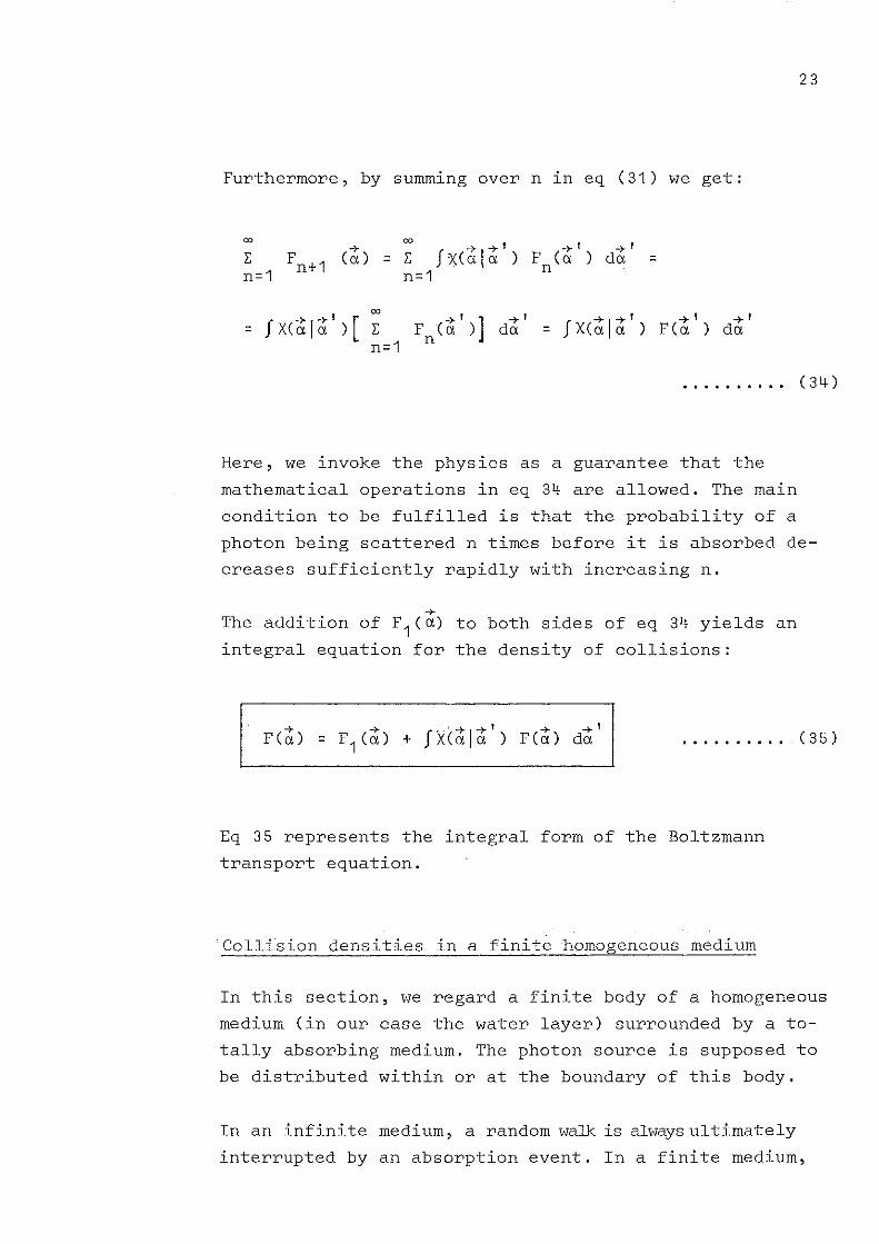
Furthermore, by summing over n in eq (31) we get:
0000
+l: Fn +1 (a) =n=1
+ +'l: fx(ala)n=1
+ +' [= fX(a!a )+'
da
. .. . . . .. .. (34)
Here, we invoke the physics as a guarantee that the
mathematical operations in eq 34 are allowed. The main
condition to be fulfilled is that the probability of a
photon being scattered n times before it is absorbed de
creases sufficiently rapidly with increasing n.
+The addition of F1 (a) to both sides of eq 34 yields an
integral equation for the density of collisions:
.......... (35)
Eq 35 represents the integral form of the Boltzmann
transport equation.
Collision densities in a finitehomogeneous medium
In this section, we regard a finite body of ahomogeneous
medium (in our case the water layer) surrounded by a to
tally absorbing medium. The photon source is supposed to
be distributed within or at the boundary of this body.
In an infinite medium, arandom walk is always ultimately
interrupted by an absorption event. In a finite medium,

24
however, the random walk can be interrupted by the
escape of the photon through one of the boundary sur
faces. The partiaI collision densities F et) insiden
the finite medium therefore converge more rapidly to-
wards zero with increasing n than do the corresponding
collision densities in an infinite medium of the same atomic
composition. The conditions for the validity of eq 34
are thus more readily fulfilled for a finite body.
The reduction of the partiaI collision densities Fnet)
inside the finite body is easily demonstrated using eq
28. As soon as the state vector t., i < n, of an inter-l
action sequence in the infinite medium has its position
vector ~i at a point outside the finite body, the inter
action sequence for the latter case is definitely broken
and gives no contribution to F et). The number of interac-n
tion sequences which contribute to F et) in a finite bodyn
is reduced giving rise to reduced collision densities.
Arandom walk .. [t1
' •••• , tNl which is interrupted by the
escape of the photon through one of the boundary sur
faces of a finite medium has a probability density given
by:
. . • • • • • . •. e36)
where xetNltN_1
) is valid for an infinite homogeneous
medium and the integration is over all points ~N situa
ted outside the finite medium.
With a finite body, a primary photon from the source has
a probability of passing through the body without inter
acting.

25
This probability is given by:
+r
1outside finite body
where F1C~i) is valid for an infinite homogeneous medium
and the integration is over all state vectors ~1 with
their position vectors ~1 at points outside the finite
body.
3. Relations between collision densities and field
quantities·
The collision density FC~) is directly connected to the
doubly-differential photon fluence through the relation:
· . . . • . . . •. C37)
when the fluence is normalized to a source which emits
one photon.
+Then, for the partiaI collision density FnCa), we have:
+F Ca) =
nj1(hv)
32<jJ(n-1) (hv ,n ;~)3(hv)3" · . • • • • . • •. (38)
where <J> (n-1) is the fluence of photons which have been
scattered (n-i) times and for the density of first colli
sions, Fi
(c\:) ,
+F1 (a) = j1(hv)3 2 <jJ(0)(hV,s1;;)
3(hv)3"• • • • • • • • •• ( 3 g )
where <jJ(0) is the fluence of primary photons.

26
For a monoenergetic, point-collimated source at ;0 emit
ting photons with energy hv O and direction of flight QO'the density of first collisions is:
• • • .. • • .. •• (40)
As shown above, a simple relation connects the collision-+, . • -7
density FCa) at the space pOlnt r with the differential
fluence at the same point.
Another very useful relation connects a given field
quantity ,(;) at point; with the collision densities
at all other points:
........... (41)
where TCt) is a weight function which depends on the
field quantity ,.
The weight function TCt) in some special cases
We now return to our particular problem, Fig 1, of esti
mating field quantities at point s at the rear of a finite
homogeneous water layer. As the water layer is supposed
to be surrounded by a totally-absorbing medium, only the
collision densities inside this layer contribute to the
field quantities on the boundary surfaces.

27
..,.Parameters needed to calculate the values of T(a) are
demonstrated in Fig 3.
-+ -+ -+arr, 0, hy)
//
":J~ dA =
d
1
Fig 3: Same parameters needed for calculating the weight
function T(~) in eq 41 when the field quantity• -+
T at a pOlnt r T on the boundary surface of a plane
layer containing a homogeneous medium is required.
From Fig 3 we have
..,.r T = the point at the rear of the (water) layer for
which T is to be estimated from the collision den
sities F(~) inside the layer,
..,.0 0 = the unit vector in the direction of flight of the
incident photon,
..,.the unit vector in the direction r T - -+
r,
dA = d01~T-~12 = surface element centred at ~T perpendi
cular to nT and subtending a solid angle d0 as seen
from point ~.

28
Depending on the particular field quantity being inves
tigated, T(~) is given by one of the following expres
sions.
[. a2a[(n,nT),hV'] J
= ooJ e -Il (hv ' ) Ii:T-i: I' .--~aQ"""3""(h,...v.,..;)i----
Il (hv)hvO
• .. .. • .. •. (42)
T(~) is the probability per unit cross sectional area
that a photon with energy hv and direction of flight ninteracting at the point i: will after the interaction
->-pass through asphere centred at r T without interme-
diate interactions. (The attenuation coefficients a and
Il refer to the medium contained in the plane layer).
->-T(o,) =
-Il (hv ' ) Ii:T-i: I= e
1 6(D'-n )T
where3 2 <jl(hv' ,n' ;~T)
3(hv)3Q
.......... (43)
is the required doubly-differen
tial fluence of scattered photons.

29
(s)T = the plane fluence ~ l of scattered photons:_______________________2 _
->-T(a,) =
(44)
->- ->-where T(a,)fluence - T(a) in eq 42 and T is the plane
fluence with regard to asurface perpendicular to nO'
!_~!b§_g2~e!Y:g~ff§~§~!~~!_E!~~§_f!~§~~~_2f_~~~!!~~§g
2b2!2~~
->-T(a,) =
= cos(QT' QO) T(;)differential fluence (45)
where T(;) :; T(;) in eq 43 anddifferential fluence
with regard to asurface
is the required doubly
differential plane fluence• ->-
perpendlcular to Qo'
The weight function T(~) when T is the energy fluence
or plane energy fluence is obtained by multiplying the
integrands in eq 42 and 44 with the energy hv'. When
T is the doubly-differential energy fluence or plane
energy fluence, the weight function is obtained by
multiplying T(~) in eq 43 and 45 by hv'.
30
In the calculation of the weight function T(~) above,
it has not been necessary to make any special use of
the assumption that ~T is a point at the boundary sur
face. In fact, the calculation of T(~) in eq 41 also
holds when T is the field quantity at an arbitrary
point ~T inside the layer.
If the totally-absorbing medium which surrounds the
water layer is vacuum, slight modifications to get the
weight function T(~) are needed when T is the field
quantity at an arbitrary point outside the water layer.
E. The random selection of a value for a stochastic
variable
The name "Monte Carlo" has its origin in the use of
random numbers, this being the basic principle in all
problems in which Monte Carlo techniques are used.
Although the determination of suitable methods of ge
nerating random numbers is the most basic problem in
the use of Monte Carlo methods, we will not discuss
it here, but will simply assume that we have access
to a suitable method with which we can randomly draw
numbers p in the interval (0,1) in such away that
they are evenly distributed across the interval. The
numbers p are called random numbers. The method with
which they are drawn yields a frequency function g(p)
= 1 for these numbers.
Programmes to generate random numbers are available
for most computers. As an alternative, tables of ran
dom numbers can be used.
To be able to generate random walks for photons, it is
necessary to select randomly discrete values from the
ranges of possible values of a number of stochastic

31
physical parameters such as, for instance, the scatte
ring angle in a scattering event. Although picked at
random, the selection must not be arbitrary. The se
lection procedure is necessarily determined by the
frequency function of the stochastic variable in
question.
In the following is described how such selection proce
dures or sampling methods can be constructed with the
aid of random numbers. In using random numbers, the ba
sic problem of randomness is brought back to the gene
ration of these numbers. It will be shown here how ran
dom numbers with a rectangular frequency function can
be used to construct sampling methods for a stochastic
variable with an arbitrary frequency function.
1. Discrete stochastic variables
The outcome of a selection made to determine the type
of interaction process is a discrete stochastic variable.
With probabilities P1 = ,/~, P2 = 0CbH/~ and P3 = 0INCOH/~,
the interaction is a photoelectric absorption, a coherent
or an incoherent scattering. A procedure for selecting
the outcome of an interaction process must (in order to
simulate the underlying physics) have the property of
yielding a certain process, i, with a probability equal
to p ..l
As a mere general case, suppose that a discrete stochastic
variable can take on n different values (n different events
may occur) with probabilities P1' .... 'Pn. A straightforward
procedure to sample from this stochastic variable is the
following:
The interval (0,1] is divided into n parts with lengths
equal to P1'····'Pn: 0<x~P1' P1<x~P1 + P2'···· and P1 +... + Pn-1<x~P1 + ••.• + Pn' Arandom number p is drawn
and the value i (the event i) is chosen if P1 + ..•• + Pi-1
<P'P1 + ..•• + Pi'

32
The above selection procedure yields the value i (event i)
with a probability given by:
fg(p) dp = p.l
... +p. 1. l-
as desired.
2. Continuous stochastic variables
. • . .. • • . •• (46)
The angle through which a photon is scattered in a scat
tering event and the free paths of photons between in
teractions are continuous stochastic variables.
To be able to simulate the basic physics, a procedure
to select randomly a discrete value from the range of
a continuous stochastic variable must yield a probabi
litY of drawing a value in the interval (x, x+dx) which
is equal to f(x)dx, where f(x) is the frequency function
of the stochastic variable.
Two standard methods, the distribution function method
and the rejection method, for sampling from a one-dimen
sional continuous stochastic variable are described.
The distribution funation method
The distribution function, F(x), for a stochastic variable
with frequency function f(x) is given by:
xF(x) = f f(x') dx'
-00.......... (47)
F(x) is assumed to increase monotonically from O to 1
while x increases from -00 to +00.
33
A sampling method can now be defined as follows:
1) Arandom number p is drawn.
2) Put
p = F(x) (48)
and determine the corresponding value of x, which can
be written formallyas:
x=F_ 1 (p) (49)
Here, F_ 1 is the inverse function of F.
With this selection procedure, the probability of
selecting a value in the interval (x, x+dx) is, as
desired, given by
g (p) dp = dp = f( x) dx
since, from eq 48,
dp _ dF(x) - f(x)dx - dx -
This is illustrated ln Fig 4.
• • • • • • • • •• (5 O)
.......... (51)
For example, it can be seen from Fig 4 how the interval
dp of the range of random numbers increases with increa
sing values of f(x). When f(x) is large for some x, the
corresponding interval dp is also large and so is the
probability of drawing a value in the interval (x, x+dx).

34
F(x) = p
dF(x) =
1
x x+dx
dx = f(x) dx.I
x
Fig 4: The probability of drawing a value in the inter
val (x, x+dx) is given in the distribution func
tian method by g(p) dp = dp = dF(x) = f(x)dx.
The rejection method
A disadvantage of the distribution function method is
that the calculation of the inverse function F_1 (p),
eq 49, can in some cases be very tedious. For instance,
this methad is not very suitable for the selection of
a scattering angle from the Klein-Nishina distribution
while, on the other hand, the choice of the free path
between successive interactions is well adapted to its
use.
The rejection method requires that the stochastic vari~
able can anly take on values within a limited interval.
Its use is demonstrated in Fig 5.

35
f(x)
L
o
- --lIII
- -'i- tI II Ill Il I,
ItI al
Pla a
Fig 5: Selection of a value for the stochastic variable
X, with the frequency function f(x), using the
rejection method.
The stochastic variable, X, is assumed to take on values,
x, in the interval O ~ x ~ a only. In addition, the maxi
mum value of the frequency function f(x) in this inter
val is assumed to be equal to L.
A sampling method lS defined as follows:
1) Two random numbers P1
and P2
are drawn.
2) Put
. . . . . . . . .. (52)
and determine if
If this is the case, x 1 is taken as the value for X.
If not, i.e.
(53)
.. . • .. • • •• (54)
then x1 is rejected as the value for X and the proce
dure starts again from (1).
36
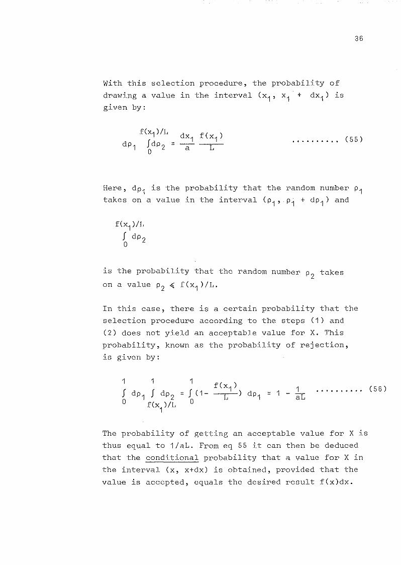
With this selection procedure, the probability of
drawing a value in the interval (xi' xi + dx1 ) is
given by:
.......... (55)
Here, dP1 is the probability that the random number Pi
takes on a value in the interval (Pi' Pi + dP1) and
is the probability that the random number P2
takes
on a value P2 ( f(x1 )/L.
In this case, there is a certain probability that the
selection procedure according to the steps (1) and
(2) does not yield an acceptable value for X. This
probability, known as the probability of rejection,
is given by:
1
= f (iD
f(x1
)L )
1= 1 - aL. . . . . . . . .. ( 56)
The probability of getting an acceptable value for X is
thus equal to i/aL. From eq 55 it can then be deduced
that the conditional probability that a value for X in
the interval (x, x+dx) is obtained, provided that the
value is accepted, equals the desired result f(x)dx.

37
Modifieation of the pejeetion method
If the probability ofrejection is large, the method
will be very time-consuming. A more rapid selection
procedure can then be constructed by combining the
rejection method with the distribution-function
method.
For this purpose, an auxiliary frequency function g(x)
suitable for the distribution function method is de
fined over the same interval O ~ x ~ a as f(x).
The sampling method is as follows:
1) Two random numbers P1 and P 2 are drawn.
2) Determine
• • • • . • . • .• ( 57)
where G(x) is the distribution function corresponding
to the frequency function g(x).
3) Determine if
. . . . . . . . .. ( 58)
where
.......... (59)
and L' is the maximum value of h(x) in the interval
o ~ x ~ a.
1f this is the case, the value x1
for X is accepted.
Otherwise, the value x1
for X is rejected and a new
attempt starting from (1) is made.

38
With this selection procedure, the probability of dra
wing a value in the interval (xi' x 1+dx1 ) is given by:
h(X1
)/L'
dP1 J dpZ =O
• • • • • • • • •• (60)
The probability of rejection is:
1 1 a [ h(X1 )}J d P1 J dpZ = J g (xi) 1- L I dX1 =O h(x1)/L' O
a1 ( 61)
1 1 J g(x1
) h(x1
) dX1 1 ..........= -y;-r = - L'O
If the auxiliary frequencv function g(x) does not differ
great ly from f(x), L' is a number close to one and the
probability of rejection will be small.
For particular cases, e.g. the Klein-Nishina frequency
flIDction of the scattering angle, a number of more specia
lized approaches can be found in the literature. A
good compilation of references is given by Carter and
Cashwell (1975).

39
II. The generation of random walks and their use in
estimating field guantities
A. Analogue simulation
Analogue simulation means that random walks are gene
rated according to the laws of physics, i.e., physically
determined probability and frequency functions are used
in selecting values for stochastic physical parameters.
In contrast, fictitious probability and frequency func
tions can be used in selecting these values. Then non
analogue random walks are generated. The important use
of nonanalogue random walks is treated in section B.
1. On the generation of random walks
Arandom walk is generated as follows:
(1) The position, energy and direction of flight of a
photon from the source at its first interaction are se
lected from the frequency function F1(~)' With a mono
energetic point collimated source, only a selection of
the position is needed. The energy and direction of
flight at the first interaction are not in this case
stochastic parameters. In addition, the selection of
position for the first interaction is identical to se
lecting a value P1 from the free path frequency func
tion f(p):
.......... (62)
This selection is best made using the distribution func
tion method. The solution of eq 49 (with x = P1) then
becomes:
1VChv) tn (1-p) .......... (63)

40
The free path frequency function in eq 62 is valid
for an infinite homogeneous medium. For a finite me
dium a test is made to see if the selected value P1
results in position coordinates ~1 = (x1 , Y1' z1)'
where:
· . (64)
outside the medium. This corresponds to the photon
leaving the medium without interacting and the random
walk is terminated. Otherwise, the random walk is con--+
tinued with its first state vector ~1 given by:
· . (65)
The fact that a photon can pass through a finite medium
without interacting can alternatively be considered in
the following way. It is first decided if the photon
will interact in the medium or else just pass through
it. With probability:
p.l
(66)
the photon interacts in the medium and with probability
(1- Pi) it escapes. The decision is made using the method
described above for sampling from a discrete stochastic
variable. p is the maximum free path inside the medium.
If it is decided that the photon interacts in the me
dium, the free path P1 before the interaction is selec
ted from a truncated normalized free path frequency
function:
f(p) · . (67)

41
The relation between the random number p and the free
path Pi is then:
• • • • • • • • •• ( 6 8 )
(2) Once the point of interaction has been selected,
the type of interaction process is determined. For
photons of energies < 1 MeV, the possibilities are pho
toelectric absorption, coherent and incoherent scatte
ring.
If photoelectric absorption is indicated, the random
walk is terminated (provided the emission of K-fluore
scence photons can be neglected).
(3) If the result of (2) is that scattering takes place,
the next step is to select the direction of motion ~n+i
and the energy hVn +i of the scattered photon.
The direction of motion ~n+i is determined by the scatte
ring angle S = polar angle in the coordinate system ins
which the direction of motion of the interacting photon
is taken to be the z-axis, and the azimuthal angle, ~s'
in the same coordinate system.
If the interacting photon is unpolarized the scattering
angle, Ss' is selected from a frequency function:
[da (S)] [da(S) . Jf(S) = dS la. hv = dn 2w slnSla hv
. n n
.......... (69)
and the azimuthal angle, ~s' is selected from a rec
tangular frequency function in the interval [0,2w]:
f( ~)1= 2w' O ~ ~ ~ 2w .......... (70)

.. • • . • .. •• (71)
42
The next step is to determine the energy hVn +1 of the
scattered photon from the frequency function:
da (8 s )J1 dn
hVn
where f(hv 18 s )d(hv), is the conditional probability that
a photon scattered through the polar angle 8s has energy
in the interval d(hv) around hv.
Selection of the energy of the scattered photon is un
necessary when there is a one-to-one relationship between
the energy of the scattered photon and the angle through
which scattering takes place.
If a distinction between coherent and incoherent scatte
ring has been made in (2), the choices of scattering
angle 8 s and energy hV n +1 of the scattered photon are
made from frequency functions f(8) and fChvi8s) in which
the total scattering cross section a is replaced by the
cross section, aCOH or aINCOH' of the scattering pro
cess in question.
The choices of the direction of motion and the energy
of the scattered photon can also be made in the opposite
order. The appropriate frequency functions are then
given by:
fChv) = [da(hV) la]d(hv) hV
n
.......... (72)
and fC~) as above.
da(hv +1)]2n sin8 1 d(hV~ hv
n
(73)
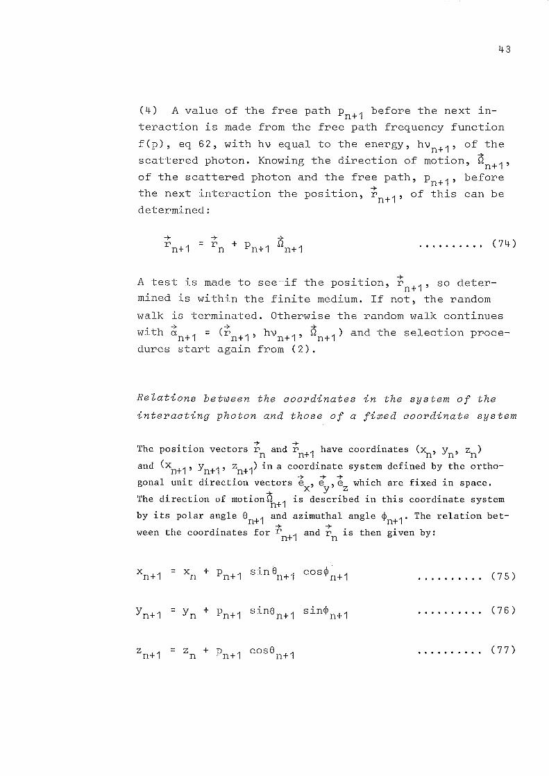
43
(4) A value of the free path Pn+1 before the next in
teraction is made from the free path frequency function
f(p), eq 62, with hv equal to the energy, hv n +1 , of the
scattered photon. Knowing the direction of motion, Qn+1'
of the scattered photon and the free path, Pn+1' before
the next interaction the position, ~n+1' of this can be
determined:
• • • • • • • . •• (74 )
A test is made to see if the position, ~ l' so deter-n+mined is within the finite medium. If not, the random
walk is terminated. Otherwise the random walk continues
with ~n+1 = (~n+1' hv n +1 , Qn+1) and the selection proce
dures start again from (2).
Relations between the coordinates in the system of the
interacting photon and those of a fixed coordinate system
~ ~
The pos1t10n vectors r and r 1 have coordinates (x , y , z )n n+ n n nand (xn+1 ' Yn+1' zn+1) in a coordinate system defined by the ortho-
gonaI unit direction vectors ~.,;,~ which are fixed in space.x y zThe direction of motionQn+1 is described in this coordinate system
by its polar angle 8n+1 and azimuthal angle ~n+1' The relation bet-• -+ -+. .
ween the coord1nates for r n+1 and r n 1S then g1ven by:
......... , (75)
.......... (76)
.......... (77)

lflf
The direction of motion nn+1 was selected by picking a polar angle Ss
and an azimuthal angle ~ in a coordinate system in which the di-srection of motion of the interacting photon, n , lies along the
nz-axis. Now, a relation between the angles Sn+1' ~n+1 and Ss' ~s
is to be derived.
rec-
can be
has
is described by a polar angle Sn and azimuthal angle ~nin
+ + + *nate system e , e , e . The unit direction vector ~~ thenX y z
tangular coordinates (sine cos~, sine sin~, cose ) asn n n n n
The derivation is based on the fact that the direction of motion nnthe coordi-
seen from fig 6.
" " ,
cosSn
en-.....
~
"~n "
" I
-- --- ~,,~Isine sin~n n
I
I sine/ n
.,.e
y
cas~n
Fig 6: The direction n is described by the polar angle S andn n
the azimuthal angle ~n' The unit direction vector nnhas rectangular eDordinates (sine cas~, sins sin~ , case ).
n n n n n
In the coordinate system in which n defines the z-axis the orthon
gonal base vectors are called -e " -e' and ~ '. The uni t directionX y z
vector i'i 1 has coordinates (sine cas~, sine sin~, case) inn+ S S S S S
this system. Now the coordinates for the unit vectors t x ', ty', t z '

45
-+ -+ -+in the eoordinate system e, e , e are to be determined. Ifx yzthese are known, the values of en+1 and ~n+1 ean then be deri-
ved from the relation:
Qn+1 sines-+ ,
sines sin~-+ , -+ ,
= cos~s e + e + coses ez =x s y
sinen+1 cos~n+1-+
sin8n+1 sin~n+1-+
cosen+1-+
= ex + €ly + e z
....... ... (78)
-+ , -+ -+ -+The coordinates for e in system e , e , e are the same as those
Qz x y z
for . Q-+ , The ehoiee of the direetion of the base vee-s~nce = e .-+n n z
tor e ' in the plane normal to Q is arbitrary. It is ehosen tox n
lie the projeetion of-+
in Qn' Hgalong e the plane normal to 7.z
-+e
-+'z Q-+' / =ee / n z
x /,I
I I 8I
sine I
ni eI ('- •cose
n
intersectcion with-+thecplane_ d.et·ilie? by ex and
intersection with the planenormal to Qn
Fig 7: The plane defined
the projeetion of
-+by e-+ ze in
Z
'* +,.and ~'t • e 1S ehosen ton x
the plane normal to Qn
lie along-+,ez
The direetion of
perpendieular to
-+,e
ythe
-+ -+ -+is then fixed. €ly' lies in the plane ex-eyprojettion of Q in this plane, Hg 8.
n

46
+'projeetion of ex
<P n
+e
y, sine
" n...'projeetion of nn
+e x
Fig 8: The base vector ~y' in the plane defined by ~x and ~y
From figs 6 - 8,+ +vectars e I, e lx y
are given by:
it fol1ows that
and + , in theez
the coordinates of the base. ~ + +
coordlnate system ex' ey , ez
= (sinen eos<pn , sine sin<p, ccse )n n n
(79 )
By b. . +, +,su stltutlng e ,ex y
in eq 78 one finds:
and + , d' t f +ez
expresse III erms o e x'
• • • • • • •• •• (8 O)
sillen+1 sin<pn+1 = - sines eos<ps eosen sill<Pn - sines sin<ps eos <p +n
+ cose· sine sin<Pn ........... (81 )s n
cosen+1 = sines eos</> sine + cose cose .......... (82)s n s n

47
The value of the polar angle en +1 is easily determined from
eq 82. The azimuthal angle ~n+1 can be found using either
eq 80 or eq 81. However, from these equations, simpler expres
sions can be found. These are:
sine sin~s ssinen+1
cose - eose eose +1S n n
eos (~n+1 - ~n) =--S=-l'"n""'e'n----=s"'i-=n"'e-n-+-
1-=:.-:.
..........
(83)
(84)
2. The use of random walks in estimating field quanti
ties
There are many different ways of estimating the values
of field quantities from simulated random walks. The
only requirement imposed on a stochastic estimate is
that it is unbiased.
Here, attention will again be directed towards the slab
penetration problem diseussed above. Field quantities
of scattered photons at points on the slab surfaees
are to be determined.
In what follows, three different estimators are deseri
bed. They are distinguished from one another by the
amount of analytieal ealculation they eontain. They
will here be called the direet simulation estimator,
the last event estimator and the collision density
estimator.
The direct simulation estiamtor
This estimator does not use any analytical calculations.
The field quantities are estimated in a straightforward
manner similar to the estimation made from a physieal
experiment. The mean value T of the field quantity ,
over a finite area, the "target area" AT' is the para-

4-8
meter that can be estimated in this way. The target
area corresponds to the detector in a physical experi
ment.
The estimator is constructed as follows: arandom walk
[->- ->- ->- 1 . .a 1 'u 2 ' ...• ,aN lS generated and a partlcular parameter
CTAT )* is allocated a numerical value according to:
- '" ->- ->- ->-CTAT ) = tCaN) if the transition a ->- aN .n-i
is such that the photon passes
through the target area AT and
for all other random walks.
tctN) is a function (defined below) of the direction
of motion nN and the energy hV N contained in the state->-vector u
N.
(TAT)'" is an estimate of the parameter CTAT ) normalized
to a source which emits one photon. Tt is a stochastic
variable: if the experiment of generating arandom
walk and allocating a numerical value to (TAT)'" as
described above is repeated, there is a large probabi
litY of getting a different value.
- '"The symbol (T~) can have three different meanings which may be
confusing. This is, however, accepted practice and one gradually
learns to distinguish among them. They are:
1) CT~)* is a function of the random walk
- '"2) CT~) is a number, viz., the value of function 1) as found in
the experiment under consideration
3) C -T~)'"."' is a stochastic variable. The number referred to in 2)
can be considered to be the result of an observation of this
variable.

49
The function t(tN
) = t(hV N, n N) depends on the particu
lar field quantity T which has to be estimated.
1. T .~fluence:
. . . . . .. . .. (85)1
!cos(Qo,nN )!
where nO is a direction vector perpendicular to the
target area AT'
2. T = the differential fluence:
1
.......... (86)
when 3 2 Hhv',n')3(hv)3>l
is the desired differential
fluence.
3. T = the plane fluence:
. . . . • . . . .. (87)
4. T = the differential plane fluence:
.......... (88)
when is the desired differential
plane fluence.
For estimating energy fluences and plane energy fluences,->- •t(aN) lS taken from eqs 85 - 88 by multiplying with the
energy hvW

50
Eqs 86 and 88 do not really give numerical values of->-
tCaN)' This corresponds to the fact that derivatives
cannot be estimated directly. Tt is only possible to
make estimates of differential fluences and differen
tial plane fluences integrated over finite intervals
of photon energy and direction of motion. Eqs 85 and->-
87 are then used for tCaN) with the proviso that->- •
tCaN) lS put equal to zero for all values of hV N and
n N which lie outside the intervals of these variables
considered.
- >I'Tt will now be shown that CTAT ) is an unbiased esti-
mate. To start with, an expression for the parameter
(rAT) is given:
J tChv,n)16= 211
2 Cs) :le ->-d <rpIChv,ll;r)
dChv)dQdChv)dn
.......... (89)
with tChv,n) one of the functions of energy and direc
tion defined in eqs 85 - 88 and <rCs) the plane fluencepIof scattered photons normalized to a source which emits
one photon.
Normalizing to a source which emits one photon, then:
cesses
in the
dChv)dn = the probability that
the photon after one
or more scattering pro
will emerge through the target area AT with energy
interval dChv) around hv and direction of motion
in the solid angle element dn around n.

The expectation. - '*varlable hAT)
=
- '*value, E (TAT ) ,
is thus given by:
of the stochastic
51
(90)
By altering the order of integration in eq 90 and sub
stituting hv for hVN and n for nN, the expression on
the right hand side of eq 89 is reproduced, i.e.:
.......... (91)
- .(TAT ) is thus an unbiased estimate of the parameter
TAT normalized to a source which emits one photon.
For the field quantities T diseussed above the partieular value
of the number N of the last state veetor in arandom walk has
no signifieanee in estimating the value of T. This faet makes
it possible to substitute n for ~ and hv for hvN• If, on the
other hand, one is interested in the value of T for photons
seattered a eertain number, a, of times, then t(~) = O for all
values of N sueh that (N-1) i a.
by:
Starting from the expression for the
in eq 90 the variance, V[(TAT)*], of- '*variable (TAT ) is immediately given
V[(i'AT )"'] =hV O
dA JO
expectation value
the stochastic
d(hv)dQ +
JQ=2'IT
d(hV)dD]
.......... (92)

52
Finally, another expression for the variance can also
be given:
v[C~År') *] ~
00 -+ _ 2
= l.: J.. .5[tC~)<- TAr]N=2
(93)
The integrations in the first sum on the right hand
side of eq 93 are to be made over all interaction-7 -7-7
sequences a i , .... , aN_i' aN such that the transition-+ -+ • '. . •a N- i -7 aN results ~n photons em~rglng from the slab.
• -7In thls case, tCa
N) = O for all sequences other than
those which result in emergence through the target area
AT' The integrations in the second sum are made over-7 -7
all sequences a i , .... , aN with all their position vec--+ -+ -+-+
tors r1
, •••. ,rN
within the slab. FCaN, .... ,a i ) TChVN)/)lChVN)
is the probability density that a photon from the source
will follow the sequence of interactions described by-+ -+ • -+a i , .... , aN and end with photoabsorptlon at r N.
[i-5FiC~)d~1 is the probability that a source photon will
emerge from the slab without any interaction.
Values of the variance are as difficult to determine
analytically as values of the expectation value itself.
Furthermore, this expectation value must be known be
for e the variance can be calculated using one of the
eqs 92 and 93.
Even values of the variance have thus to be estimated
from experimental data. An estimate of the variance
can be established only if more than one random walk
is generated. In cases when H random walks are generated,
53
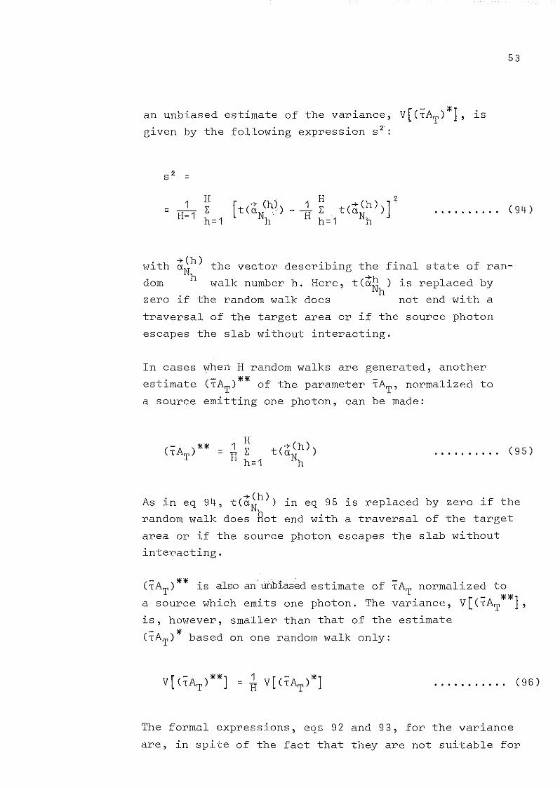
an unbiased estimate of the variance, V[CTAT )*}, is
given by the following expression S2:
1= H-1
HEh=1
• • • . . • • . .• C94)
with
dom
zero
+Ch)aN the vector describing the final state of ran-
h walk number h. Here, tctnh) is replaced by
if the random walk does not end with a
traversal of the target area or if the source photon
escapes the slab without interacting.
In cases
estimate
a source
when H random walks are generated , another- ** -CTAT ) of the parameter TAT , normalized to
emitting one photon, can be made:
1 H= - E
H h=1.......... (95)
. +Ch)As ln eq 94, tCaN ) in eq 95 is replaced by zero if the
random walk does Rot end with a traversal of the target
area or if the source photon escapes the slab without
interacting.
CTAT ) ** is also an' urlbiased estimate of :rAT normalized to
a source which emits one photon. The variance, V[CTAT**],is, however, smaller than that of the estimate
- *CTAT ) based on one random walk only:
........... (96)
The formal expressions, eqs 92 and 93, for the variance
are, in spite of the fact that they are not suitable for

54
calculations of variances, useful in finding methods
to reduce variances. Different methods of reducing
variances will be discussed later. First, however,
two other estimators are described.
The last event estimator
Immediately prior to its last interaction in the slab,
the state of a photon describing arandom walk [~1""
.. , ~N-1' ~NJ is given by either the vector ~N-1 or+
by aN' depending on whether the random walk is termina-
ted by the escape of the photon from the slab or by+
photoelectric absorption at a point r N within the slab.
The last event estimator is constructed as follows:
arandom walk [~1""" ~N-1' ~N] is generat ed and a
parameter T* is allocated a numerical value according
to:
+
*TCaN)
T = +qCaN)
+
*TCa
N_
1)
T = qCtiN
_1
)
*T = O
when the random walk is terminated by
photoelectric absorption in the slab,
when the random walk is terminated by
escape of the photon from the slab and
when the source photon escapes the
slab without interacting.
The function T depends on the particular field quantity
T for which an estimate is to be made. It is a function
of the position, the energy and the direction of motion
immediately prior to the last interaction. It is, how
ever, independent of the particular value of N and is
identical to the function TC~) defined in eqs 42 - 45.

55
The function q is also independent of the particular
value of N. q = qct) is the probability that a photon
involved in an interaction characterized by state vec
tor t has its final interaction in the slab.
T* is an unbiased estimate of the field quantity T
normalized to a source which emits one photon. This
will now be shown.
Normalizing to a source which emits one photon, it can
be stated that the slab collision density FCt)dt times->-
qCa) equals the probability that a photon from the
source will interact Cpossibly after one or more scat
tering processes) in the slab described by a state vec-• -7- -+- • •
tor in the lnterval da about a such that thlS lnterac-
tion is its final one within the slab. The expectation
value, ECT*), of the stochastic variable T* can then
be written:
->-ECT*) = f TC~) FCt)qCt)dt = fTCt)FC;i)dt = T
q Ca,)
.......... (97)
->The integration in eq 97 is over all state vectors a
with position coordinates within the slab. The second
*equality follows from eq 41. Thus T is an unbiased
estimate of T normalized to a source which emits one
photon.
The variance,
be written:
* ~VCT ), of the stochastic variable T can
= f [
= f
->-TCa)
->-qCa)
1T ct) ]~_->-
qCa)
->- ->- 2FCa,) da, - T C98)

56
with the last equality coming from the fact that
= the probability that a photon from the source is
absorbed photoelectrically in the slab or escapes
from the slab Cpossibly after one or more scattering
processes) and hence equals one.
A . ** f . h l . b bn estlmate T o T Wlt ower varlance can e o -
tained by generating H random walks and calculate
the arithmetic mean of the H values for the stochastic
variable ,*found. The variance, VC,**), of the esti-**mate, is then given by:
. • . • . . . . .• C99)
By generating H random walks, an unbiased estimate S2
of the variance VC,*) can be made with S2 given by an
expression equivalent to that in eq 94.
The absorption estimator
The probability q is the sum of the probability that
the photon is scattered and then escapes the slab
without further interactions and the probability that
it is absorbed photoelectrically. The probability of
scattering followed byescape from the slab may be
difficult to calculate. The last event estimator can
be modified to take account of the probability of
photoelectric absorption only. The estimate ,* of ,
is then:
*,
*, = O
when the random walk ends
with photoelectric absorp
tion in the slab and
for all other random walks.

57
The proof that this modified estimate is also unbiased
follows from eq 97 with qC~) = TChv)/~Chv).
The variance of the modified estimate is, however,
different:
-+* f[ TCa)VCT ) = T(hv)7~(hv)-+da +
.......... (100)
Here, eC~) is the probability that a photon which in
teracts as described by the state vector t is scattered
and leaves the slab without further interactions.
A comparison between eqs 98 and 100 shows that the
variance of the modified estimate is the greater one
since TChv)/~Chv) < q(~). The modified estimator yields
a value of zero for the estimate more often. In compen
sation, the values different from zero must be compara
tively larger. This contributes to alarger spread in
the values obtained with the modified estimator.
difficulty associated with
that the function T(a) -+ 00
Since T(~) is contained in
the last event
as I1\T - 1\ I -+ O,
the variance in
A particular
estimator is
eqs 42 - 45.
quadratic form, eqs 98
infinite value for the
and 100,
variance
this may
*VCT ). A
result in an
method to avoid
an infinite variance is instead to make an estimate of
the mean value, T, of the field quantity averaged over
a finite area AT' The estimate is then given by:
when the random walk ends
with photoelectric absorption,

58
1JA
+
ATT(a
N_
1)dA
-'" T when the random walks endsT = +q(aN- 1 ) with the escape of the photon
from the slab and
when the source photon escapes
the slab without interacting.
The estimate T* is a stochastic variable with a limited
range of possible values, the upper limit being set
by the size of the area AT'
The difficulty with the unIimited range of values of
the stochastic variable T'" vanishes if the slab lS
surrounded by vacuum and field quantities T for points
at a certain distance from the slab are required.
Certain modifications of the function T(&) have then
to be made. The estimation of T can otherwise proceed
ln the same way.
The collision density estimator
This estimator makes use of the information from all
the state vectors in arandom walk. It is constructed
f [ + + J .as ollows: a random walk a 1 , .... , aN lS generated
and a parameter T'" is allocated a numerical value
according to:
'"N +
T = l: T(a. )i=1 l
'"N-1
+T = l: T(ai)
i=1
'"T = O
when the random walk ends
with absorption in the slab,
when the random waIk ends
with escape of the photon
from the slab,
when the source photon escapes
the slab without interacting.
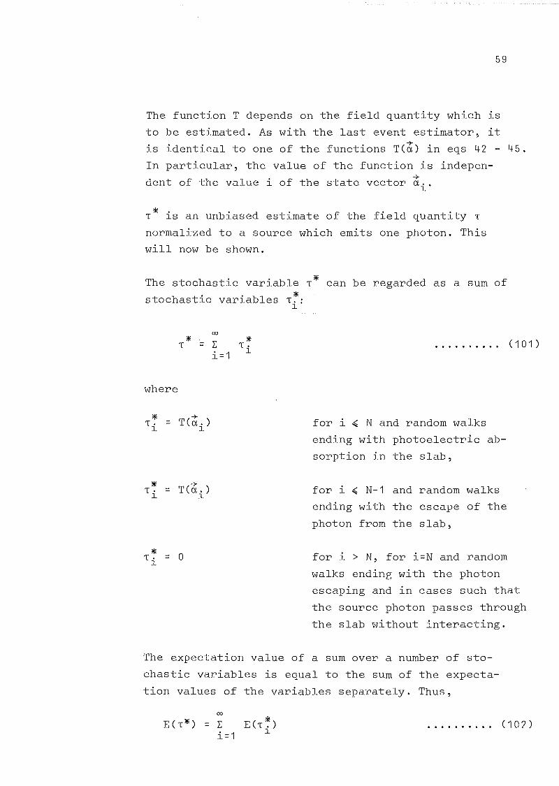
59
The function T depends on the field quantity which is
to be estimated. As with the last event estimator, it
is identical to one of the functions T(~) in eqs 42 - 45.
In particular, the value of the function is indepen-
dent of the value i of the state vector ~ ..l
T* is an unbiased estimate of the field quantity T
normalized to a source which emits one photon. This
will now be shown.
The stochastic variable T* can be regarded as a sum of
stochastic variables T~:l
GO
*T = l:i=1
where
* -7-T· =T(a.)l l
>If -7-T. = T(a.)
l l
>IfT· = O
l
>I<T .
l(101 )
for i ~ N and random walks
ending with photoelectric ab
sorption in the slab,
for i ~ N-i and random walks
ending with the escape of the
photon from the slab,
for i > N, for i=N and random
walks ending with the photon
escaping and in cases such that
the source photon passes through
the slab without interacting.
The expectation value of a sum over a number of sto
chastic variables is equal to the sum of the expecta
tion values of the variables separately. Thus,
GO
E(T*) = l:i=1
,.E (T . )
l.......... (102)
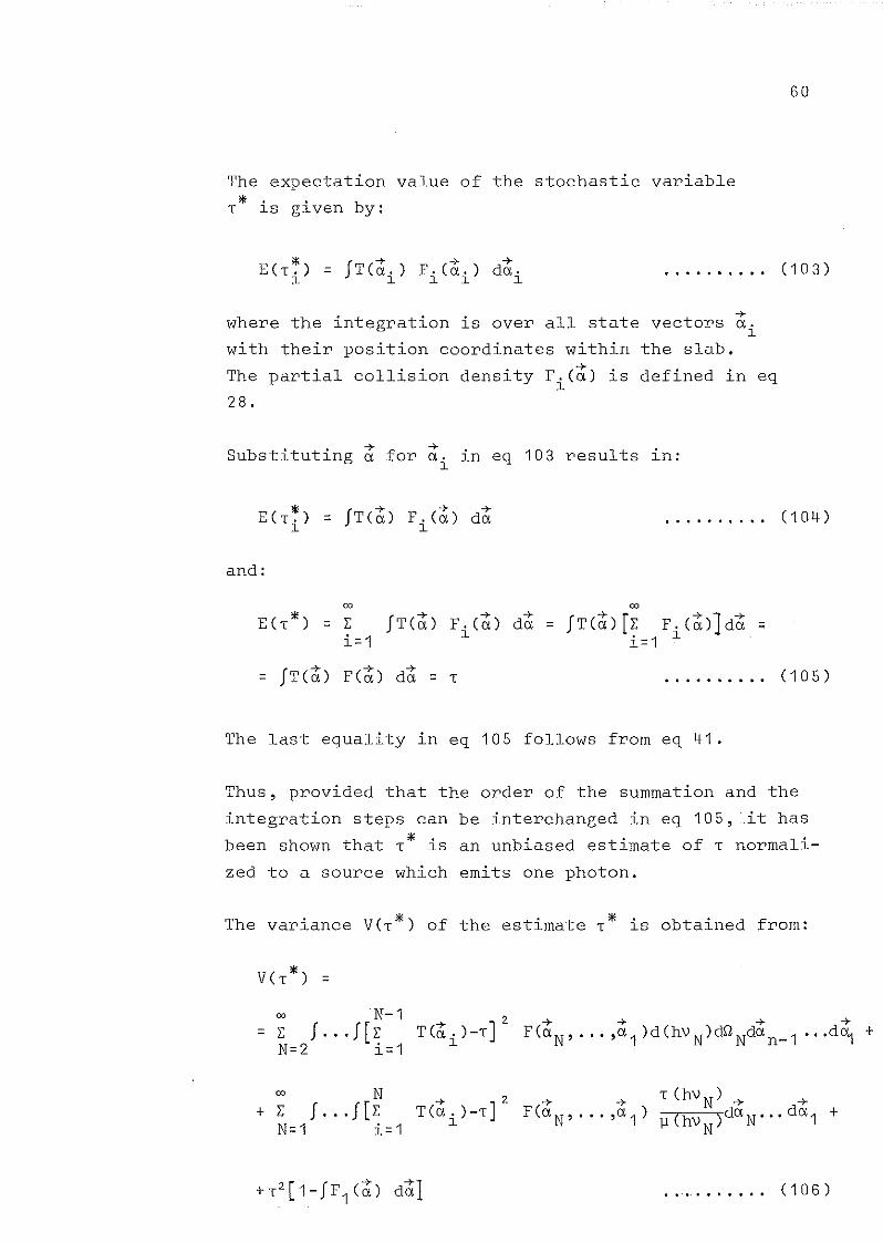
60
The expectation value of the stochastic variable"'. . bT lS glven y:
'" f + + +ECT.) = TCa.) F.Ca.) da.l l l l l
+where the integration is over all state vectors a·
l
with their position coordinates within the slab.
The partial collision density FiCt) is defined in eq
28.
+ +Substituting a for a. in eq 103 results in:
l
C1 O3)
'" fTC"t)+ + (104)ECT.) = F. Ca) da ..........l l
and:
00 00
E hl!<) fTC"t)+ +
fTC"t) [l: F.C"t)]dt= l: FiCa) da = =i=1 i=1 l
.......... (105)
The last equality in eq 105 follows from eq 41.
Thus, provided that the order of the summation and the
integration steps can be interchanged in eq 105,it has
been shown that T'" is an unbiased estimate of T normali
zed to a source which emits one photon.
The variance VCT"') of the estimate T'" is obtained from:
'"VCT ) =
00 N-1= l: f ... 5[l:
N=2 i=1
00 N+l: f ... f[l:
N=1 i=1
+ 2TCa.)-T]
l
•...••.... (106)

61
In the first sum on the right hand side of this equa
tion, the integrations are over all interaction sequen
ces which end with the escape of the photon from the
slab. In the second sum, the integrations are over all
interaction sequences which end with photoelectric ab
sorption in the slab.
The variance V(T*) can also be written formally as:
V(T*) >I< >I< '* * (107 )= V(l:T i ) = l:V(T . ) + 2l: C(T i' T. ) .......... l i<j Jl
>I< * * *where C(T., T.) is the covariance of T. and·T .• If the stochasticl J l J * *
variables are independent of one another, then C(T., T.) = O forl J
i t- j. This will not be the case here. The value taken by the state+ +
vector a. depends on the value taken by a· l'l ~
E . h' . t "'''' f . h l .ven ln t lS case an estlma e T o T Wlt ower varl-
ance than V(T"') can be obtained by generating H random
walks and forming the average of the corresponding H
b . '" ("'''')'' 9o servatlons of T . V T lS glven by eq 9 .
As in the case with the last event estimator, there is
a need even here to limit the range of possible values
of the stochastic variable T"'. This can be carried out
as described earlier by considering a finite area and
making an estimate of T averaged over this area or by
estimating T for points at a certain distance from
the slab.
3. Comparison between estimates - efficiency and precl
sion of an estimate
For any comparison between different estimates to be
meaningful the same parameter should be estimated in
each case. Using the direct simulation estimator only
the average value T of the field quantity T over a
finite area can be estimated. The last event estimator

62
and the collision density estimator can be extended
to estimate such averages. The need to limit the va
lues taken by the stochastic variable T* of the last
event and the collision density estimators for points
at the slab surfaces naturally leads to a situation
where averages T are estimated. In cases for which
the field quantity T as a function of position is of
interest, the area over which the averaging is carried
out should be chosen such that T varies only little
over this area.
From the direct simulation estimator, an estimate T* == (TAT)*/AT of T averaged over AT is obtained with the
variance V(T*) = V[(TAT)*]/AT. This variance is expli
citely dependent on the size of the target area AT'
Even the variances of the estimates obtained with the
last event estimator and the collision density esti
mator are dependent on the size of the area AT in those
cases in which such an area has been introduced.
The efficiency of an estimate
The efficiency of an estimate is usually defined as the
invers e of the product of its variance and the compu
ting time required to generate a value for it (make an
observation of it). Defined in this manner, an estimate
does not get more efficient just because it is based-*on more random walks. Thus, the estimate T is as effi-
-**cient as the estimate T equal to the average of H ob-
servations of T*. The variance V(T**) 'is H times lower-~ -*than the variance VeT ) but generating H values for T
requires H times the computing time.
While the variance is a defined function, the efficiency
will vary depending on the standard of the computer and
the competence shown in data handling.

63
The precision of an estimate
In all Monte Carlo work it is a matter of central inte
rest to establish the precision with which an estimate
of a given parameter is made. The variance is of inte
rest in judging this precision.
The most rigorous manner of stating the precision of
an estimate is to indicate a confidence interval. This
can be carried out when both the variance VCT*) and-*the type of frequency function for T are known. For
example, if T* has a Gaussian frequency function the
desired value T C= the expectation value) is with 95%
probability contained within an interval of ± 2/VCT*)
about the experimentally obtained Cestimated) value-* -*for T • If, however, T has a different frequency func-
tion the same relation will not hold. A knowledge of
the variance only is not sufficient to determine the
precision.
Furthermore, the variance is initially not known. It
can, however, easily be estimated from experimental
data as has already been referred to above. The fol
lowing expression S2 always yields an unbiased esti
mate of the variance VCi*) independent of the frequency
function for T"':
. 1 H [S2 = H-1 ~ Th
h=1.......... (108)
Here, H is the total number
in the experiment and Th
is
from the h:th random walk.
of random
the value
walks generated-!I<
for T obtained
Though S2 is in all cases an unbiased estimate of VCT~),
the precision of this estimate will in turn depend on-il( -lIE
the type of frequency function for T • If T has a
Gaussian frequency function, S2 is the best estimate of

64
VCT~) and a knowledge about H and S2 allows the construc
tion of confidence intervals by means of the Etudents
t-distribution. With a frequency function for T* which
lS very unsymmetrical, it is, however, to be expected
that S2 will provide an estimate of VCT*) with a much
poorer precision and there is no general method of con
structing confidence intervals.
Returning to the concept of the efficiency of an esti
mate, this is intended to be a measure of the computing
time needed to get an estimate with a certain precision.
As has been pointed out above, it is not quite correct
to judge the precision from the variance only. Judging
it from the estimated variance S2 is still more compli
cated. On the other hand, it is difficult to find a bet
ter quantity to use which is still practical. It should,
however, be kept in mind that the estimated variance S2
only serves as a very crude measure of the precision.
Comparison between estimators
The last event estimator makes use of the analytically
calculated probability per unit area that the photon
after its last interaction emerges from the slab through
a certain point. This probability is contained in the
function TC~). The collision density estimator extends
this use to include the sum of the escape probabilities
after each interaction. The estimates obtained with the
last event estimator and the collision density estimator
therefore take on values equal to zero with a frequency
much less than the corresponding estimate obtained with
the direct simulation estimator. In the latter case,
only the random traversals of the target area AT give
nonzero values for the estimate.
A general rule is that any increase in the degree of ana
lytical content in estimates tends to decrease the value

65
of the variance. This seems intuitively correct. How
ever, to show this formal ly by comparing expressions
92 and 93 for the variance with the corresponding
expressions 98 and 106 appears to be impossible. With
the direct simulation estimator, the estimate takes a
value of zero more frequently while with the other two
estimators the ranges of those values which differ
from zero are often larger, for instance in estimating
plane fluences. In estimating fluences, however, even
the direct simulation estimator yields estimates with
an infinite range of possible values due to the factor
eos (QO,QN) in the denominator of t(~N)' eq 85. To avoid
infinite variances in this case, a cut off value for the
angle (QO' QN) is usually introduced.
Even if it is true that the last event and the collision
density estimators produce estimates with lower varian
ces than the direct simulation estimator, the former
need not be the more efficient ones. The analytical
calculations contained in the estimates of the last
event and collision density estimators require a compu
ting time which can be used to generate a greater number
of random walks if the direct simulation estimator is
used. As the variance of an estimate varies inversely
with the number of random walks used for the estimate,
it may weIl be that, from the point of view of the pre
cision attainable, it is more profitable to use a given
computing time to generate as many random walks as pos
sible using the direct simulation estimator rather than
to generat e fewer random walks and use the last event
or the collision density estimators.
The collision density estimator requires the calculation
of more values of T(~) than the last event estimator
which only uses one such value. On the other hand, a
value of q(~) must be calculated with the last event
estimator but not with the collision density estimator.
When q(~) includes both the probability of photoelectric

66
absorption as weIl as the probability of scatteringfollowed byescape from the slab, the calculation of
q(&) can be expected to require considerable computing
time.
The last event estimator can, as has been described
above, be modified to take account of the probability
T/~ for photoelectric absorption only. The analytical
effort in making the estimate is then strongly reduced.
The variance, however, increases compared to the variance
of the unmodified estimate using q(&). This increase is
greater the more T/~ deviates from q(&). In cases when
the probability of photoelectric absorption is large
compared to the probability of scattering followed by
escape, the modified last event estimator can, however,
be expected to be more efficient than the unmodified one.
The question as to which estimator is the most efficient
cannot be answered in a general manner. The estimators
must be experimental ly tested for their efficiences from
case to case. Generally, the direct simulation estimator
is favoured if symmetries in the geometry of the problem
can be used to get large target areas, as in the parti
cular slab penetration problem discussed here. The other
estimators can be expected to be less dependent on such
geometrical symmetries.
B. Nonanalogue simulation
In the above, three different estimators have been
described, the most efficient of which can be selected
for use in any particular situation. The efficiency of
any particular estimator can further be increased by
using fictitious probability and frequency functions
in selecting values for stochastic physical parameters.
The increase in efficiency is due either to a reduction
of the computing time needed to obtain an estimate or

67
to a reduction in the variance of the estimate.
The optimal choice of fictitious probability and fre
quency functions is dependent on both the irradiation
geometry and the estimatar used. This will be illust
rated in the section on importance functions. In selec
ting the most efficient Monte Carlo scheme for solving
a given problem, on has thus to weigh different esti
mators toghether with different fictitious frequency
functions, which is usually a matter of great complexity.
Before proceeding to describe the use of random walks,
generated with the aid of fictitious probability and
frequency functions, a particular topic relevant to
the pencil beam slab penetration problem shall be dis
cussed.
Methods of obtaining a desired precision in estimates
at different points
In the pencil beam slab penetration problem presented
above, different field quantities were to be determined
as a function of the position on the rear of the slab.
This means that Monte Carlo estimates of the field
quantities have to be made for many different point s
on the rear of the slab.
It is here possible to use one and the same random
walk for making estimates at different points.
This has two advantages compared to generating a new
random walk for each estimate. Computing time is redu
ced and the estimates at different points are corre
lated, i.e., the integral of the field quantity over
the rear of the slab is determined with greater pre
cision than is the case when different random walks
are used for the estimates at different points.

68
The precision desired in the estimate at any given
point can be attained by basing it on a sufficiently
large number of random walks. A disadvantage arises
if widely different numbers of random walks are needed
to obtain the desired precision for estimates at dif
ferent points. The correlation between the estimates
then disappears.
This disadvantage can be treated by nonanalogue simula
tion. By using randomwalks generat ed with nonanalogue
simulation, the variance of an estimate at a certain
point can be reduced. This often implies that estimates
at other points, using the same estimator and random
walks, get an increased variance. The optimal choice of
fictitious probability and frequency functions depends
not only'bn the estimator butålso on the point at which the
field quantity is to be determined. One can thus try to
optimize the estimate for each point separately. Then,
however, different random walks have to be used for the
estimates at different points and the advantages of
using one and the same random walk for making all the
estimates are again lost.
The fact that a given set of fictitious probability and
frequency functions reduces the variance of the estimate
at one point but increases it at another can, in this
context, be used positively. One may be able to find a
set of functions such that the required precision is
attained at all point s when the estimates at these points
are all based on the same set of random walks.
This can be illustrated by discussing estimates of the
plane fluence with the direct simulation estimator. The
probability per unit area that a photon from the source
will after scattering emerge through a point at the
rear of the slab decreases rapidly with the distance
from the axis of symmetry (the pencil beam). If p is the
probability that a photon emerges through a particular
69
target area AT' the expected number of photons which
traverses this area is Np when N photons are emitted
from the source. The variance in the number of photons
passing the area is in this case Np (1-p) and the rela
tive standard deviation is given by [N p (1_p)]1!2 !Np == ~pIINp. The precision (expressed a~ the relative
standard deviation) in the estimate of the plane fluence
thus decreases rapidly with increasing distance from
the pencil beam (decreasing value of p) when the esti
mate at each point is based on the same number, N, of
random walks. Since target areas in the form of annular
rings (with cylindrical symmetry) can be selected in
this case, p does not decrease so rapidly with the dis
tance from the pencil beam as does the probability per
unit area. Sufficiently far away, however, the estima
tes must be based on alarger number of random walks to
attain the same precision.
By introducing fictitious probability and frequency
functions, the probability that a random walk ends with
the photon passing through an annular ring far away
from the pencil beam can be increased while, at the same
time, the probability that it ends with the photon pas
sing through an annular ring near the pencil beam is
reduced. As a net result, the precision in the estima
tes at different points will be equalized.
1. On the generation of random walks with nonanalogue
simulation
Here, arandom walk will be generated by the same se
quence of selection procedures (1) - (4) as was used
in the generation of random walks with analogue simu
lation. The difference is that, in choosing values for
the stochastic variables involved, fictitious probabi
litY and frequency functions may be used. The choice
of the photon's position, energy and direction of
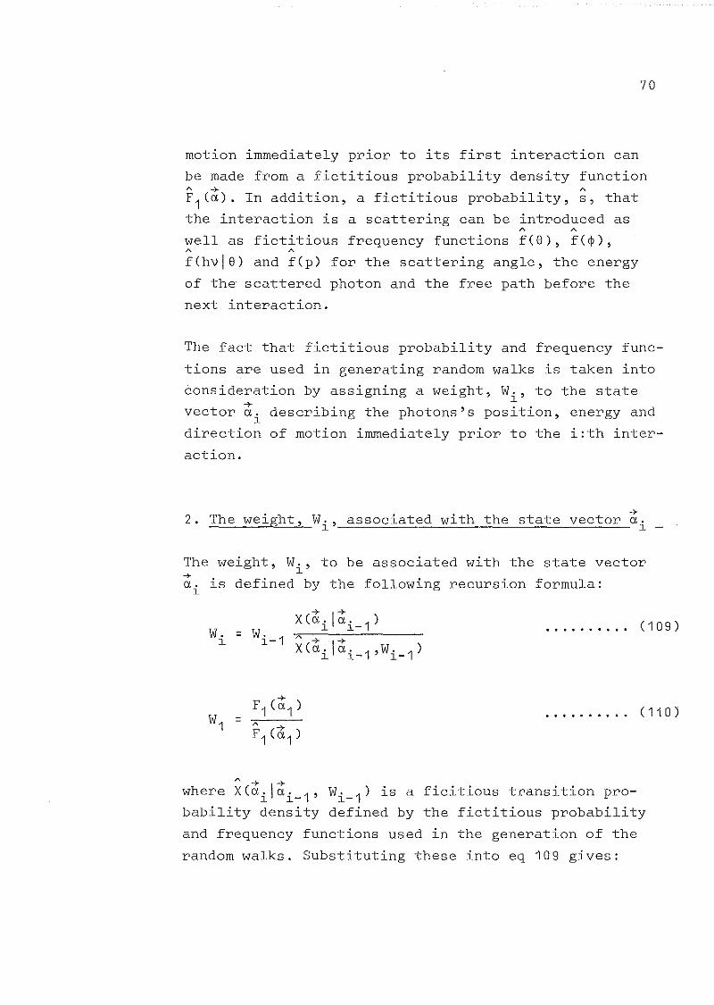
70
motion immediately prior to its first interaction can
be made from a fictitious probability density functionA + A
F1 (a). In addition, a fictitious probability, s, that
the interaction is a scattering can be introduced asA A
well as fictitious frequency functions f(8), f(~),A A
f(hvI8) and f(p) for the scattering angle, the energy
of the scattered photon and the free path before the
next interaction.
The fact that fictitious probability and frequency func
tions are used in generating random walks is taken into
consideration by assigning a weight, W., to the statel
vector t. describing the photons's position, energy andl
direction of motion immediately prior to the i:th inter-
action.
+2. The weight, Wi , associated with the state vector a i
The weight, W., to be associated with the state vectorl
t i is defined by the following recursion formula:
W. = W. 1l l-
+ 1+X(a. a. 1)l l-
A + 1+X(a. a. 1'W, 1)l l- l-
.......... (109)
.......... (110)
where X(~·I~· l' w. 1) is a ficitious transition pro-l l- l-
bability density defined by the fictitious probability
and frequency functions used in the generation of the
random walks. Substituting these into eq 109 gives:

71
w. =l
= W. 1l-
W. ·>1l~
W. 1l-
[fce )fCep )fChv·le )]h [fCp=I;';·-i'<1 1)]hVs s l S v. 1·. l l •l- l
[A A A ] [A ->- ->- JfCe )fCep )fChv·le ) ->- fCp=lr.-r. 11) ->-s S l S 0,. 1 l l- 0,. 1
l- l-
W. 1l-
tiol
hv.l
W. 1l-
tiol
hv.l
.......... (111)
where fCp),fCe),fCep) and fChv[e) are the frequency func-A A A
tions defined in the eqs 62 and 69 - 71, f Cp) ,fCe) ,fCep)
and fChv[e) are the corresponding fictitious frequencyA A A
functions. S =a/~ and S = a/~ are often referred to as
the true and the fictitious survival probabilities.
If a distinction between coherent and incoherent scat
tering has been made in generating the random walks
the following relation is useful in calculating theweight W.:
l
fCe )fCep )fChv. [e ) =s S l S
+
72
where fINCOH and f COH are the frequency functions
obtained by substituting 0INCOH and 0COH foro in
the eqs 69 - 71.
As incoherent and coherent scattering through a par
ticular scattering angle (es'~s) can never result in
the same energy hV i of the scattered photon, one of
the terms on the right hand side of eq 112 must always
be equal to zero.
The fictitious transition probability density
X(tilti_1,Wi_1) has here been described as depending on+
the weight W. 1 associated with the state vector a. l'l- l-
This does not mean that it is necessarily dependent on
this weight but only that it could be. There exists a
great variety of possible ways to choose the fictitious
probability and frequency functions. In particular, they
may depend on other parameters than those relevant in
physics. This has been indicated in eq 111. The ficti-A
tious survival probability s may, for instance, not only
depend on the photon's energy but also on its position,
its direction of motion and its weight.
Although there exists a great range of possibilities
in choosing the fictitious probability and frequency
functions, there are also requirements which have to
be imposed on these functions. These will be discussed
later.
The recursion formula for the weight Wi , eqs 109 and
110, shows that the weight associated with the state+ . fvector a i depends on all the prevlous state vectors o
the random walk:
.......... (113)

73
By expanding the recursion formula, the following
expression for the weight Wi is obtained:
+ +Wi = W(ui '···· ,(1 ) =
+ \+ + 1+ + 1+ +XCa i a i -1
) X(u i _1
a i _2
)· .. ·X(a2
(1
) F1
(a1
)= =
xCai \ai _ 1 ,Wi _ 1 )XCai _ 1 \ai _ 2 'Wi - 2 )···· xCa 2 \a1 ,W1 )F1 Ca1 )
.......... (114)
Eq 114 shows that the weight Wi is equal to the ratio
of the true probability density that a photon will
interact through a particular seguence of events and
the fictitious probability density that it will inter
act through the same sequence.
Comments on fictitious collision densities
A photon emitted from the source and interacting accor
ding to the laws dictated by the fictitious probability
and frequency functions has a probability density to
pass through an interaction sequence a 1 , ••• , a whichA n
is given by the function F(tn , ... ,a1).
. + +Integratlng over the state vectors a1
, •• •;,an _ 1 yields
the fictitious partiaI collision density Fn(~):
C11 5 )
A +The fictitious collision density FCa) is then given by:
A +F(a) =
00
l:n=1
C11 6 )

74-
These partiaI and total collision densities are valid
for a particular state vector a independent of the
weight associated with it.
In case the fictitious probability and frequency func
tions are weight dependent, the integral equation for
the partiaI collision density corresponding to that in
eq 30 for the true partiaI collision density must be
written:
( 117 )
A-+ A-+-+Here, F (a ,W ) is obtained by integrating F(a ,a 1'"
-+ n n n -+ n n-+... ,a1 ) not over all interaction sequences a 1 ,·· .. ,an - 1as in eq 115 but only over those sequences such that
the weight Wn has to be associated with the state vector+. +an' Eq 117 lS lntegrated over all state vectors an as
weIl as over all possible weights Wn associated with a+
particular state vector a .n
3. Estimating field quantities from random walks gene
rated with nonanalogue simulation
Here, it will be shown how the direct simulation esti
mator, the last event estimator and the collision den
sitY estimator are modified in using random walks gene
rated with nonanalogue simulation.
The direct simulation estimator
is generated and
normalized to a
follows:
A ~andom walk [a1 , .... ,aNJ(TAT )* of the parameter TAT ,
emits one photon, is made as
an estimate
source which

75
if the random walk ends with the
photon passing through the target
area and
for all other random walks
...Here, tCaN) is the same function of the energy hV N and
the direction of motion ON as defined in eqs 85 ~ 88.
The expectation_A *variable CTAT )
A '"value, E[CTAT ) ]
is given by:
, of the stochastic
C118 )
The integrations in eq 118 are over all possible inter
action sequences which end with the photon passing
through the target area. possible interaction seguences
are those for which the probability density function..... -+ -+. . A+ -+FCaN, ... ,a1 ) lS nonzero. If the functlon FCaN, ... ,a1 )
is equal to zero, this implies that the interaction... .... . f h . tsequence a 1 , ... ,aN lS not posslble or a p oton ln er-
acting according to the laws dictated by the fictitious
probability and frequency functions. Random walks des
cribed by [&1""'&NJ will then never be generated and
weights WN for such sequences are not defined.
Substituting the expression for the weight WN according
to eq 114 into eq 118 gives:
00
= ~=2 f ... ftC&N) FC&N'" "&1) dChvN) dQN d&N_1··· d&1
C119 )
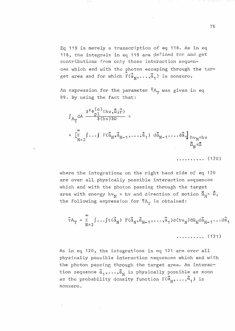
76
Eq 119 is merely a transeription of eq 118. As in eq
118, the integrals in eq 119 are defined for and get
eontributionsfrom only those interaetion sequen-
ees whieh end with the
get area and for whieh
photon eseaping through the tar-A + +F(a N, ... ,a1 ) is nonzero.
An expression for the parameter TAT
was given in eq
89. By using the faet that:
2 (s) n +a <l>pl (hv, jr) =a(hv)an
00
= [l: Joo.JN=2
.. oo ...... (120)
where the integrations on the right hand side of eq 120
are over all physieally possible interaetion sequenees
whieh end with the photon passing through the target
area with energy hV N = hv and direetion of motion nN= n,the following expression for TAT is obtained:
00
= l: J ... Jt(ciN)N=2
( 121 )
As in eq 120, the integrations in eq 121 are over all
physieally possible interaetion sequenees whieh end with
the photon passing through the target area. An interae-. ~ +.
t10n sequenee a1
, ••. ,aN
lS physieally possible as soon. + +.
as the probability density funetlon F(aN, ... ,a1 ) lS
nonzero.
77
Requipements imposed on the fiatitious ppobability
and fpequenay funations
The expressions in the eqs 119 and 121 are identical,
i. e. (i'AT)* is an unbiased estimate of :rAT' provided.. ~ ~.
that for any lnteractlon sequence u 1 ' .... ,u N WhlCh
ends with the photon passing through the target areaA + + +FCu N, .... ,u 1 ) is nonzero as soon as both tCuN) and
-+ -+FCu N, .... ,u1 ) are nonzero.
In estimating fluences and plane fluences, tC~N) is
nonzero for all values of hV N and QN' while in esti
mating differential fluences and differential plane
fluences integrated over finite intervals of energy
and direction of motion, the function tC~N) takes on
a value of zero for all energies hV N and directions
of motion QN which do not belong to the intervals con
sidered.
In estimating fluences or plane fluences, the above re
quirement on the function FC~N""'~1) means that the
fictitious probability and frequency functions must be
chosen such that:
(1) the fictitious transition probability density
xC~n+11~n'Wn) is nonzero as soon as the true transition
probability density xctn +1 \un ) is nonzero and the posi
tion vector ~n+1 indicates a point within the slab.
(2) XC~n+1\~n,Wn) is nonzero as soon as XCun+1\~n) is
nonzero and the transition results in the photon passing
through the target area.
On the other hand, in case the transition is such that
the photon escapes from the slab without passing throughA -+ -+
the target area, XCu +1\u ,W ) may be chosen equal ton n nzero although xCun+1Iun) is nonzero. Thus in generating
random walks, the photons may be prevented from escaping
78
from the slab except through the target area (or the
target areas, in cases when one and the same random
walk is used for estimates at different points). For. . .-+
instance, if a photon after an lnteractlon at pOlnt r nis given a direction of motion Dn +1 which does not point
in the direction of the target area, the decision as to
wether it will escape from the slab can be dropped and
the position ~n+1 of the next interaction be selected
directly from a truncated normalized pathlength fre
quency function, such as given in eq 67.
Furthermore, photons from the source can be prevented
from passing through the slab without interacting. The
fictitious probability density function F1(~) can be
chosen such that:
when the integration is over all
the positions ~ are contained in+must be nonzero as soon as F1 (a)
within the slab.
. . . . . . . . .. (122)
+state vectors a such that
A +the slab. However, F1 (a)
is nonzero for points
In estimating differential fluences and differential
plane fluences integrated over finite intervals of
energy and direction of motion, X(~ +11~ ,W ) may in addi-n n ntion be chosen to be equal to zero as soon as the energy
hV n +1 is less than the lower limit of the energy inter
val considered. For instance, in generating random walks,
the photons can be prevented from being incoherently
scattered such that the loss in energy results in energies
of the scattered photon below the actual limit. Further
more, if a photon interacts at ~ and is given a new di-n
rection of motion Q 1 which points towards the targetn+area but is not within the interval of direction of mo-
tion actually considered, it can be prevented from escaping.

79
It has thus been shown that some physically possible
transitions may be neglected in generating the ran-
dom walks. It may, on the other hand, be questioned
if it is possible to allow transitions which are not
physically possible. Such transitions can be allowed
but are of no interest since state vectors generated
with the aid of transition probability densities
which do not correspond to physical transitions will
have weights which are identically zero, eqs 109 and 110.
Comparison of the variances in estimates obtained with
nonanalogue and analogue simulation
Though the expectation values of the estimates are the
same, their variances will depend on wether analogue
or nonanalogue simulation has been used.
The variance, V[(tAT )1" of the estimate (tAT )* using
nonanalogue simulation is in a straightforward manner
given by:
00
• • . • . • " •• (1 23)
The integrations in the first sum are over. all interac
tion'sequences which end with the photon escaping from
the slab and t(tN) is putequal to zero if the photon
does not escape thröugh tl1etarget area. The integrations
in the second sum are over all ihteraction sequences
which are completely contained in the slab.

80
Eq 123 can be simplified to:
.......... (124)
where the integrations in eq 124 are over all inter
action sequences which end with the photon escaping
through the target area. Eq 124 follows from the follo
wing general relation valid for each stochastic variable ~:
2~
V(O = E(~2) - [E(O] (125)
The expression for the variance of the corresponding
estimate using analogue simulation, eq 93, can simi
larly be simplified to:
=
.......... (126)
where the integrations are over all interaction sequen
ces which end with the photon passing through the tar
get area.

81
As can be seen by comparing eq 124 with eq 126, the
variance of the estimate using nonanalogue simulation
differs from that of the corresponding estimate using
analogue simulation.
By a elever choice of fictitious probability and fre
quency functions, the variance in eq 124 can be made
considerably smaller than that in eq 126. In principle,
the variance in eq 124 can be reduced to zero. This
point will be treated later in the section on importance
functions.
However, a poor selection of fictitious probability and
frequency functions can easily lead to estimates with
variances much larger than in the corresponding esti
mate based on analogue simulation.
Same simple variance reducing steps
From a practical point of view, the efficiency of an esti
mate is of greater interest than its variance. It may
weIl be that it is worthwhile to use an estimate with
increased variance if thereby the camputing time is
greatly reduced. If, for instance, it is difficult to
sample from a given physical frequency function, it may
be profitable to introduce a fictitious frequency func
tion which does not depart very much from the physical
one but from which it is easy to sample.
As has been pointed out earlier, however, the efficiency
is not as weIl defined a concept as the variance. Vari
ance reduction methods can be and have in fact for a
long time been the subject of systematic studies. The
use of fictitious probability and frequency functions
with the aim of reducing the variance of an estimate
is usually called importance sampling. The importance
function, which will be treated in a following section,

82
is a very useful too l in the systematic analysis of
importance sampling. In the following only some simple
variance reducing steps will be pointed out.
It has already been anticipated that the variance of
an estimate according to the direct simulation esti
mator can be reduced to zero. From eq 123 can be seen
that, for the variance to be zero, necessary conditions
are that scattered photons are not allowed to escape
except through the target area, that photons are not
absorbed in the slab (~N = 1) and that photons from
the source are not allowed to escape without interac-A + +
ting at least once (JF1
(a) da = 1).
In other words, all random walks such that the estimate
takes a value of zero must be prevented.
Now, three steps making use of the necessary conditions
for zero variance can be indicated which obviously re
sult in a variance reduction. They contribute to increase
the frequency of all random walks which end with the
photon escaping through the target area. This in turn
means that the weights WN
in eq 124 all get smaller than
one such that the variance in eq 124 will be less than
the variance in eq 126.
A
Firstly, the fictitious survival probability s is put
equal to one. This means that all interactions are con-A
sidered to be scattering processes. The quotient s/s,
one of the factors in the formula for the weight, eq
111, is then always smaller than one.
Secondly, each time ascattered photon's direction of
motion does not point through the target area the pho
ton is not allowed to escape. The position of the next
interaction is chosen from a truncated, normalized free
path frequency function as that of eq 67. The ficitiousA
free path frequency function f(p) is thus defined as
83
A A
f(p) = f(p) in eq 67 for p < P and f(p) equal to zeroA
for p > P. The quotient f(p)/f(p) for use in the for-
mula for the weight, eq 111, will be smaller than one-)lPwith the factor (1-e ).
Thirdly, the free path for a photon from the source is
as weIl seleeted from a truncated, normalized free path
frequency function as that of eq 67, i.e. a photon from
the source is not allowed to esoape without interacting
in the slab. Then the weight W1 equal to the quotient+ A +
F1 (a)/F1
(a) will be a number smaller than one. For the
pencil beam slab penetration problem W1
will be equal
to 1-e-)ld where d is the thickness of the slab.
The step of putting the fictitious survival probability
equal to one is always variance reducing. The choice of
a truncated, normalized free path frequency function is,
however, more critical. If it is not chosen as above a
general statement of variance reduction cannot be made.
If for some values of p the quotient f(p)/f(p) may get
equal to a number greater than one the weights WN may
also get greater than one for some random walks. With
the choice of truncated, normalized free path frequency
functions according to eq 67 one is assured that theA
quotient f(p)/f(p) is always less than one independent
of the value of p.
For the varlance to be zero all random walks must end
with the photon passing through the target area and
for each random walk the estimate must take a value
equal to TAT . If, for instance, the plane fluence is
the field quantity to be estimated, t(~N) is equal to
one for all ct N. The weights WN should then take on a
value equal to TAT for all random walks. With the va
riance reducing steps described above all random walks
end with a traversal of the target area but the esti
mate will hardly be equal to TAT for each random walk.
Though obviously variance reducing and fulfilling the
necessary conditions for zero variance the steps are

84
not sufficient to reach this ideal situation. Moreover,
the ideal fictitious probability and frequency functions
will depend on the particular field quantity to be esti
mated.
Comments on the weight WN
assooiated with a photon esca
ping from a finite medium
4-The weight WN associated with the state vector aN of a
photon escaping from a finite medium can be described in
two different ways. These will be discussed here.
The definition of the weight given ln eq 114 indicates
that the weight WN associated with an escaping photon
is strictly given by:
00
ff(p)dpP
........... (127)
Here P is the distance from the point ;N-1 of the last
interaction to the boundary of the medium in the direc
tion QN of the escaping photon and the fictitious freeA
path frequency function f(p) is defined for an infinite
homogeneous medium.
A
The fictitious free path frequency function f(p) must
not be explicitely defined for p > P. In generating a
random walk a decision can first be made whether the
photon escapes or not. With probability

85
00 A
J f(p)dpP
it escapes. If the decision is that the photon does
not escape, the position of the next interaction is
selected from a truncated, on the interval [O, pJ
normalized free path frequency function.
Another way to take account of the escape probability
is first to select a value of the free path before the
next interaction from a free path frequency functionA
f(p) valid for an infinite homogeneous medium and then
to test if this ends in a point outside the finite me
dium. If this is the case, the random walk is inter
rupted. Now, one could think of associating a weight
W~ with the escaping photon according to:
w! =N
.......... (128)
where ~N is the position of that interaction which
would have occurred if the finite medium was replaced
by an infinite homogeneous medium.
-;- -;-With functions FCaN, ... ,a1 )
for an infinite homogeneous
A -;- -;-
and FCaN, ... ,a1 ) defined
medium, the weight W~ can
W! =N
alternative ly be written:-;- -;-
FCaN, ... ,a1 )
A -;- -;-
FCaN,···,a1 )
.......... (129 )
When weights W~ Crather than WN) are associated with
the state vectors ~N of escaping photons the expecta-

86
tion value of the estimate is given by:
. . . . . . . . .. (130)
where F(~N""'~1) is defined for an infinite homogeneous medium and the integrations are over all inter-
action sequences such that ~N describes a point outside-7
the finite medium and the transition from state a N- 1-7-
to state aN in the infinite medium involves a traver-
sal of the target area.
ISubstituting the expression for WN in eq 129 gives:
00
= L: J. .. Jt(~N)N=2
.......... (131)
h ( -7- -7- ) • •w ere F a N , ... ,a1
lS valld for
medium and the integrations are
an infinite homogeneous
performed as in eq 130.
Eq 131 can be rewritten in the following form:
00
= L:N=2
J.. .Jt(&N) [ JF(&N"" '~1 )dVN J d(hvN)
;N outside finite medium
.......... (132)
87
The expression for the expectation value in eq 132
is identical to that in eq 119.
It has thus been shown that the expectation value of
the estimate will not be changed when using weightsI
WN rather than weights WN according to eq 127. The
variance will, however, depend on the particular weights
used. An increase of the variance can be expected as at
result of using weights WN
rather than weights WN.
This will now be shown.
The weights WN
are weighted
according to the relation:
tmeans of the weights WN
C1 33)
where
neous
tians
A + +. .FCaN, ... ,a1 ) lS deflned for an infinite homoge-
medium and the integrations are over all posi
~N outside the finite medium.
I
Using weights WN ' the variance will be given by:
C1 34)
~ ~ ~
where FCaN, ... ,a1 ) is defined for an infinite homogeneous
medium and the integrations are over all interaction se
quences such that the transition from state &N-1 to
state &N in the infinite medium involves a traversal of
the target area.
The following expression is then valid for the difference• I •
between the variances using welghts WN and welghts WN:
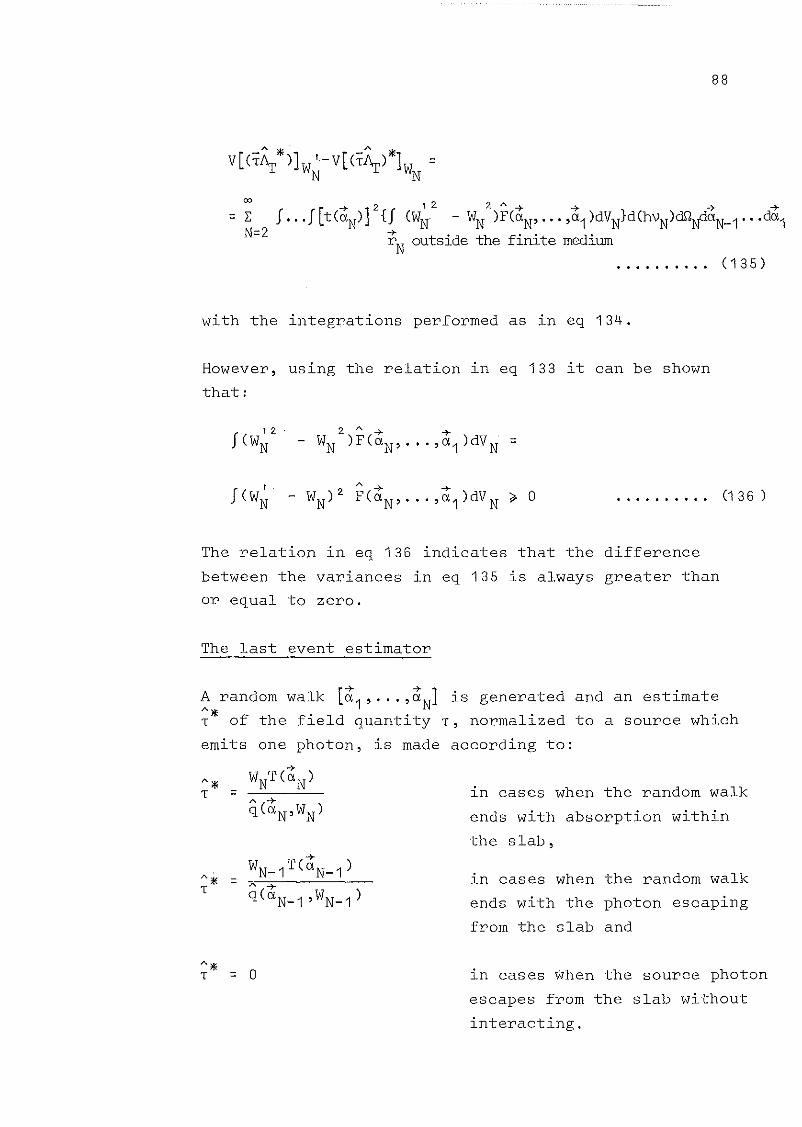
88
ro
= l:N=2
-+ 2 ,2 2.1'\-+ -+ -+-+f .. .f[tCClN)] {f cWN - wN )FCClN"" ,Cl1 )dVN}dChVN)cKltfClN_1" .dCl1r
Noutside the finite medium
.......... C135 )
with the integrations performed as in eq 13~.
However, using the relation in eq 133 it can be shown
that:
f CW~ C1 36 )
The relation in eq 136 indicates that the difference
between the variances in eq 135 is always greater than
or equal to zero.
The last event estimator
A random walk [t1
, ... ,tN
J is generated and an estimateAll'T of the field quantity T, normalized to a source which
emits one photon, is made according to:
-+A* WNTCCl N)T = A -+
qCClN,wN)
-+
Al'W
N_
1TCCl
N_
1)
= Ä -+T qCClN
_1
,WN
_1
)
All'T = O
in cases when the random walk
ends with absorption within
the slab,
in cases when the random walk
ends with the photon escaping
from the slab and
in cases when the source photon
escapes from the slab without
interacting.

89
Here, T is the same function as was used in the corres
ponding estimate using analogue simulation and ~Cdi,Wi)is the fictitious probability that a photon which inter
acts described by state vector ~. associated with weightl
Wi has its last interaction within the slab.
A",The expectation value, ECT ), is found from:
EC~"') =
00
= l:N=1
00
+ l:N=2
C1 37)
A
where C1-s) is the fictitious probability that an inter-A
acting photon is absorbed and e is the fictitious proba-
bility that the photon is scattered but escapes from
the slab after the scattering.
The integrations in eq 137 are over all interaction-+ -+ -+ -+ • •
sequences a1
, ... ,aN
and a1
, ... ,aN
_1
WhlCh Ile as a whole. . A-+ -+ [A-+ ]wlthln the slab. Then FCaN, ... ,a1 ) 1-sCaN,WN is the fic-
titious probability density that a photon goes through a
random walk [~1""'~N] which ends with absorption at ;N'
while FCdN_1 , ... ,d1 ) ~CaN_1,WN_1) is the fictitious pro
bability density that a photon goes through a random
walk [a1""'~N] which ends with escape from the slab
after the interaction at ~N-1'
The second sum on the right hand side of eq 137 can be
rewritten:
00
l:N=2
J.•.J

= 1:N=1
J...J
90
.......... (138)
By substituting eq 138 in eq 137 and uSlng the relation:
.......... (139)
one finds:
+00 WNTCaN) A + + A + + +
= 1: J... J FCa N,···,(1 ) qCaN,WN) daN' ... da 1A +N=1 qCaN,WN)
00
J... J + ........ -+- ~ -+ -+ -+= 1: WNTCa N) FCaN,···,(1 ) daN' ... da 1N=1
.......... C1I+0)
The integrations in eq 140 are over allinteraetion sequen
ees t1' .... ~N lying as a whole within the slab. It should
be noted, however, that if qC~N,WN) is equal to zero, the
eorresponding interaetion sequenee gives a zero eontribu
tion to the integrals due to the faet that if qC~N,WN) is
equal to zero, no random walks will be generated sueh that
a photon deseribed by state veetor ~N assoeiated with
weight WN has its last inte~action in the slab. Furthermore
interaetion sequenees with FC~N""'~1) equal to zero do
not eontribute to the integrals. No sueh interaetion se
quenees will ever be generated and weights WN for these
sequences are not defined. In eonsequenee, the integrations
in eq 140 are limited to those interaetion sequenees suehA-+-+ A -+
that both FCa N, ... ,( 1 ) and qCaN,WN) are nonzero.
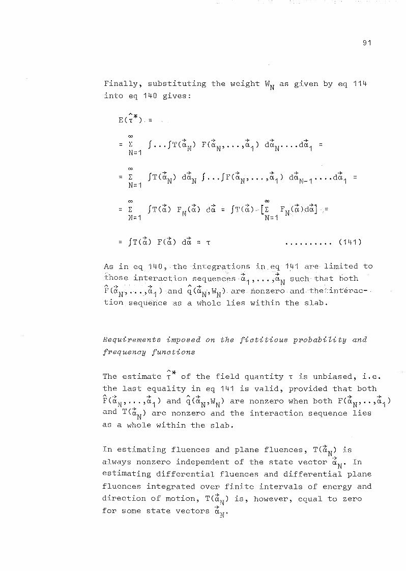
91
Finally, substituting the weight WN as given by eq 114
into eq 140 gives:
00
00
fT(~N)-7 f -7 -7 -7 -7
= E daN ... f FCaN,··· ,a1 ) daN_1 ··· . dO'. 1 =N=1
00 00
fTC~)-7 -7
fTC~) [E FNC~)d~J= E FNCa) da = =N=1 N=1
As in eq 140, the integrations in eq 1.41 are limited toh . '. -+-+
t ose ~nteract~on sequences a1 , ..• ,aN such that bothA -+ -+ A -+. . .F Co: N, ... ,0: 1 ) and q Co: N·, WJ\f) are nonzero and :thetlnt·erac-
tion sequerice as a whole lies within the slab.
Requirements imposed on the fictitious probability and
frequency functions
The estimate ~* of the field quantity T is unbiased, i.e.
the last equality in eq 141 is valid, provided that bothA -+ -+ A -+ -+ -+FCaN, .. . ,a1 ) and qCaN,W
N) are nonzero when both FCaN, .. ,a1 )
and TC~N) are nonzero and the interaction sequence lies
as a whole within the slab.
In estimating fluences and plane fluences, TC~N) is
always nonzero independent of the state vector ~N' In
estimating differential fluences and differential plane
fluences integrated over finite intervals of energy and
direction of motion, TC~N) is, however, equal to zero-7
for some state vectors aN'

Thus, in estimating
physically possible
fluences and plane fluenees, all., -+ -+ •
transltlons a. +a. 1 whlch dol l+not involve an escape from the slab must for all va-
92
lues of the weight Wi also be possible for photons
interacting according to the laws dictated by the
fictitious probability and frequency funetions. However,
in contrast to the case with the direct simulation esti
mator, it is permitted to prevent all transitions which
end with the photon escaping from the slab. On the other
hand, a photon which interacts as described by state
vector~. and which is prevented from escaping (~(~.,W.)=O),l l l
cannot as well be prevented from being absorbedA -+ A A A
(s(a.,W.) = 1), since the probability q = 1 - s + el l
that the photon has its last interaction in the slab+
must, independent of the weight W., be nonzero when T(a.)l l
is nonzero.
A physically possible transition ~l + ~i+1 implies
that the survival probability s(hv.) is nonzero. Thel
fictitious survival probability ~(a.,W.) must then alsol l
be nonzero to make the corresponding transition in the
fictitious world possible. If ~(ai,Wi) is equal to zero,
all interactions are absorptions and the photon has no
further interactions.
If, however, differential fluences and differential
plane fluences integrated over finite intervals of
energy and direetion of motion are to be estimated,A +sCa.,W.) may be put equal to zero as soon as the energy
l l .
hv. is less than the lower limit of the energy intervall
considered. The value of TCa.) in the estimate is thenl
zero and will remain so for all the following state
vectors of arandom walk.
In estimating differential fluenees and differential plane+
fluences TCai ) may take values equal to zero although
the energy hV i is above the lower energy limit eons ide
red. This will be the case when the direction defined
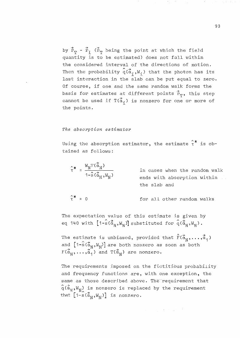
93
->- ->- ->-by r T - r i (rT being the point at which the field
quantity is to be estimated) does not fall within
the considered interval of the directions of motion.
Then the probability q(~.,W.) that the photon has itsl l
last interaction in the slab can be put equal to zero.
Of course, if one and the same random walk forms the
basis for estimates at different points ~T' this step
cannot be used if T(~.) is nonzero for one or more ofl
the points.
The absorption estimator
Using the absorption
tained as follows:
A*estimator, the estimate T is ob-
in cases when the random walk
ends with absorption within
the slab and
for all other random walks
The expectation value of this estimate is given byA + A +
eq 140 with 11-s(C!N,WN)1 substituted for q(C!N'WN),
The estimate is unbiased, provided that F(~N'" "~1)
and [1-~(aN,WN)1 are both nonzero as soon as both->- ->- ->-F(C!N, ..• ,a1 ) and T(C!N) are nonzero.
The requirements imposed on the fictitious probability
and frequency functions are, with one exception, the
same as those described above. The requirement thatA ->-q(aN,WN) is nonzero is replaced by the requirement
that [1-~(~N,WN)1 is nonzero.

94
Comparison of the variances in estimates obtained with
nonana~ogue and ana~ogue simu~ation
The variance, VC~*), of an unbiased estimate ~* using
the last event estimator is given by:
vci*) =.
00
=LN=1
C142)
The variance, VC,*), .of the corresponding estimate ,*
using analogue simulation is given in eq 98 but can,
for camparison, be rewritten in the form:
00
= L J... JN=1
.......... (143)
The integrations in the eqs 142 and 143 are made over•• -7 -+- • •
all lnteractlon sequences a 1 , .•. ,aN
whlch lle as a
whole within the slab.
Using the absorption estimator, the corresponding varian
ces are given by the last expressian in eq 142 and by
[A+ 1 A+
eq 143 with 1-scaN,WN) substituted for qCaN,WN) and
[1-sChVN
)} substituted for qCaN
). Since all random walks
which end with the photon escaping from the slab give
estimates equal to zero the expressian next to the last

95
one ln eq 142 lS not valid even if [1-~J is substitutedA
for q.
Using nonanalogue simulation, the variance ln the esti
mate, eq 142, can as in the case with the direct simu
lation estimator be reduced to zero. A zero variance
can also be obtained using the absorption estimator.
Comments on variance reduction
From eq 142, it can be seen that a necessary condition
for the variance to be zero is that no source photons
are allowed to pass through the slab without interac
ting in it. Using the absorption estimator, an additional
requirement for zero variance is that no photons are
allowed to escape from the slab. All random walks such
that the estimate takes a value of zero must obviously
be avoided.
In the pencil beam slab penetration problem, an obvious
variance reducing step is to choose the point for the
first interaction from a truncated normalized free path
frequency function such as that in eq 67. If nothing-~delse is changed, the weights W
Nare all equal to (1-e )
and the varlance in eq 142 is smaller than the variance
in eq 143.
Using the absorption estimator, the variance is further
reduced if all free path frequency functions are trun
cated and normalized according to eq 67.
Using the last event estimator and preventing the photons
from escaping as above does not only mean that the weights
WN all get smaller than one but also that the probability
that a photon has its last interaction in the slab de-A ~ A +
creases. With q(aN,WN) less than q(a N), it may weIl be
that the quotient WN
/q(~N,WN) in eq 142 takes a value

96
larger than the quotient 1/q(~N) in eq 143, even
although WN is a number less than one. In this case,
no general statement on variance reduction can be
made.
Another way of getting values smaller than one for all
the weights WN
would be to increase the survival pro
bability, i.e., to put ~ > s. This step does not,
however, usually lead to a reduction of variance. The
fictitious absorption probability [1-~(~N,WN)J to be
used with the absorption estimator, is in this case
smaller than the true absorption probability [1-s(hVN)],
counteracting the effect of reducing the weights to num
bers smaller than one. The fictitious probabilityA +q(aN,WN) that a photon has its last interaction in the
slab, to be used with the last event estimator, may be
both smaller and larger than the corresponding true+
probability q(aN).
The values T(~N)/q(~N) taken by the estimate using the
last event estimator and analogue simulation will vary
considerably. In particular, if the interaction point
~N is close to the point ~T for which the estimate is+made, T(aN) lS large.
In order to get zero variance, the estimate must take
on a value equal to T for each random walk. Using non
analogue simulation, the estimate is given by+ A +
WNT(aN)/q(aN,WN). To ensure that the value of this para-A +
meter is a constant, the quotient WN/q(aN,WN) should,
roughly speaking, be small when T(&N) is large and large
when T(tN) is small.
This goal cannot only be reached by changing the values
of the survival and escape probabilities, the only steps
that have so far been discussed. The shapes of the fre
quency functions for the scattering angle and the free
path before the next interaction can also be varied. If

97
the latter steps are taken, the fictitious probabilityA + +
density F(aN, ... ,a1 ) can also acquire values conside-
rably larger than that of the true probability density
F(~N""'~1) for some interaction sequences, while at
the same time the converse is true for other sequences.
The weights can in this way be influenced independent
of the values assumed for the survival and escape pro
babilities. A proper balancing of the quotient WN/q(~N,WN)
against T(~N) is to befound by the combined use of all
the different ways of varying the weights WN (including
changes of the survival and escape probabilities).
+ +Using analogue simulation, interaction sequences a 1 , .. ,aNwhich result in large values of the parameter
[T(~N)]2 /q(~N) give a large contribution to the variance
in the estimate, eq 143. An attempt to decrease the vari
ance by using nonanalogue simulation (importance sampling)
will primarily be an attempt to get small values for the
corresponding weights WN by increasing the probability
density for these interaction sequences. This must be
done in such away that the weights associated with the
state vectors of other interaction sequences are not
allowed to increase too much. Otherwise, the result may
even be an increased variance. Importance sampling, i.e.,
a proper balancing of the weights together with the sur
vival and escape probabilities, is a sensitive matter. A
thorough knowledge ot the behaviour of radiation in matter
is extreme ly valuable to enable favourable results to be
obtained.
Comment on a simple scheme for nonanalogue simulation
using the last event and the absorption estimators
Using analogue simulation, the variance in the estimate
of the absorption estimator is larger than the corres
ponding variance of the last event estimator. However,
the last event estimator requires the calculation of the

98
probability q that a photon has its last interaction
in the slab. This calculation may be so time consu
ming that the last event estimator need not necessa
rily be more efficient than the absorption estimator.
Using nonanalogue simulation, it is possible to pre
vent the photons from escaping both when the last
event estimator is used and when the absorption estima
tor is used. If this is the only change that is made,
the estimates of the last event estimator and the ab
sorption estimator are in fact identical. Provided
that the photons are prevented from escaping in a
straightforward manner using truncated normalized free
path frequency functions as given by eq 57, this step
is variance reducing so far as the absorption estima
tor is concerned, but the same is not necessarily true
for the last event estimator, as was discussed above.
As the calculation of the escape probability is dropped
uSlng the last event estimator and the variance is 10
wered by using the absorption estimator, it may weIl
be that this estimate is more efficient than the esti
mates of both the last event estimator and the absorp
tion estimator when analogue simulation is used.
The collision density estimator
Arandom walk is generated and an estimate T~ of the
field quantity T normalized to a source which emits
one photon is made according to:
+W.T(a.)
l lin cases when the random walk
ends with absorption within
the slab,
N-1+= L W.T(a.)
. 1 l ll=in cases when the random walk
ends with the photon escaping
from the slab and

All'T = O
99
in cases when the source photon
escapes without interacting in
the slab.
T(~i) is the same function of ~i as is used in the
corresponding estimate using analogue simulation.
Here, the expectation value, E(;"'), is given by:
00
A '"=l: E(T i )=i=1
00
00
f~ ~ ~
= l: T(a.) F.(a.) da. =i=1 l l l l
00
fT«;:)·[l: Fi (&'")] d&'"=i=1
f~ ~ ~
= T(a) F(a) da = T .. . . . .. ... (144)
The integrations in eq 144 are over all interaction-7- -+- ., • •
sequences a 1 , ... ,a i WhlCh lle as a whole wlthln theA ~ ~
slab and are such that F(a i , ... ,a1 ) is nonzero. The
last equality is valid, i.e. the estimate is unbiased,
provided that F(~i""'~1) is nonzero as soon as both
T«;:.) and F«;:"""(;:1) are nonzero. The requirementsl l
imposed on the fictitious probability and frequency
functions are the same as with the last event estima-A
tor, except that the probability q that the photon has
its last interaction may be equal to zero although both~ ~ ~
T(a i ) and F(a i , ... ,a1 ) are nonzero.

The varlanee,A~ A~
VCT ), in the estimate T is given by:
00 N-1= l: J...J [l:
N= 2 i=1
00 N+ l: J... f[l: W.TC;.)
N=1 i=1 l l
..........
The integrations in the first sum on the right hand s ide
of eq 145 are over all interaetion sequenees whieh end
with photons eseaping from the slab while the inte
grations in the second sum are over all interaetion se
quenees whieh lie as a whole within the slab.
The expression for the varianee, eq 145 Can be rewor1<e d
to give Cef eq 125):
VC~*) =
00 N 2
= l: f ...J[l: W.TC&:.)] FCt'N'''''&:1)N=1 i=1 l l
..........
The integrations in eq 146 are over all interaetioYL .--.sequences whieh lie as a whole within the slab and q
..;-t:: Sis the fietitious probability that the photon has --
last interaetion within the slab.
eq 106, can f =:c-'
In a similar manner, the expression
variance using analogue simulation,
parison be reworked to ~ive:
for the corres P c:> J:'. CC(

101
= ZN=1
f f[ N C+)J 2 C+ + ) C+ ) + + - ,2... L/ a i F ~, ••• 'CY'1 q ~ d~ ••• •da1
•.•••• o·, ••• (14-7)
From eq 14-5, it can be seen that if source photons are
not allowed to travers e the slab without interacting
and if interacting photons are neither allowed to be
absorbed nor to escape from the slab after the inter
action, the variance will be zero. However, if photons
are neither allowed to be absorbed nor to escape, no
random walk will ever be terminated. This makes the
method unreasonable. The probability q that a photon
has its last interaction in the slab must be nonzero+
for at least some state vectors aN' so as to make pos-
sible the termination of random walks. It is then, how
ever, no longer possible to show that the variance in
the eqs 14-5 and 14-6 can be reduced to zero. This dis
tinguishes the collision density estimator from the
direct simulation estimator and the last event estima
tor. With the latter two estimators it can be shown
that the variance in the estimate can, using nonanalogue
simulation, be reduced to zero.
Comments on variance reduction
As with the last event estimator, in this case importance
sampling primarily means that interaction sequences
~1"" '~N giving large contributions [ZTCui )]2 to the
variance using analogue simulation, eq 14-7, should be" . A-r -+ -+ ~
examlned ln more detall, FCaN, ... ,(1 ) larger than FCaN, .. ,(1 )
so that the weights W. of these sequences become small.l
This must, however, be done in such away that the weights
of other interaction sequences are not allowed to increase
too much, since this may again result in an increased
variance.
Large values for
from long random+state vectors a.
l
the estimate, ZTCai)' can originate both
walks and from short ones which include+giving large values for TCa i ).

102
4. Examples of fictitious probability and frequency functions
a. Fictitious survival probabilities
Analytical averaging of survival
Putting the fictitious survival probability ~ equal to unity
means that all interactions are taken to be scattering pro
cesses. If no other alterations in the scheme for generating
random walks with analogue simulation are made, the weight
W. = s1s2" .. s. 1 associated with state vector ~.l l- l
is equal to the expected number of photons surviving the in-
teraction sequence ~1""'~i-1 per photon which begins it.
Putting the fictitious survival probability equal to unity
is known as analytical averaging of survival. It means that
a random variable, the survival of an interaction, is repla
ced by its expectation value (analytical average). The choice
of the type of interaction (absorption or scattering ) is
not considered when generating random walks.
It has been shown above that analytical averaging of survi
vaI reduces the variance when the direct simulation estima
tor is used. This agrees with the rule which states that the
introduction of analytical calculations into an estimate
tends to reduce the variance.
Using the last event estimator, it could not be shown
that analytical averaging of survival is variance reducing.
Analytical calculations are already contained in this esti
mator in such away that the effect of analytical averaging
of survival is not unambigously variance reducing.
Using the collision density estimator it can, however, as
with the direct simulation estimator, be shown that analyti
cal averaging of survival is variance reducing. The analytical
calculations already contained in the collision density esti
mator are, unlike those of the last event estimator, such that
analytical averaging of survival tends to reduce the variance.

103
-;-This is due to the fact that each value EW.TCa.) taken
l l
by the estimate using the collision density estimator
together with analytical averaging of survival, con
tains a weighted average of the values ETCt.) takenl
by the estimate for a number of random walks which,
using analogue simulation, end with absorption at-;- -;- -;- C-;- ) • •r 1 ,r2 , .... or r N r N- 1 . USlng the last event estlmator
together with analytical averaging of survival, the
values taken by the estimate do not contain such ave
rages.
The variance reducing effect of the analytical avera
ging of survival can when used together with the colli
sion density estimator also be understood more intuiti
vely, in the following way. Long random walks usually
give large contributions to the variance using analogue
simulation, eq 147, since ETCt.) tends to be large whenl
N is big. Importance sampling then means that the gene-
ration of long random walks should be favoured. The
analytical averaging of survival just gives rise to the
generation of an increasing number of long random walks.
Furthermore, all weights take values less than one. The
problem of random walks associated with excessively large
weights will thus not arise.
Proof that the analytieal averaging of survival reduees
the varianee in the estimate obtained with the eolli
sion density estimator
The variance,
simulation is
* *VCT ), in the estimate T using analogue
given by:
00 NJ... f[ TCti)t
-+ -+ -+-+ -+- T2= E E FCaN'···,a1)qCaN)daN····da1 =
N=1 i=1
00 N{f .. ·fLE -7 ]2 + -+ -;- -;- -;-
= E TCai) FCaN,···,a1 ) eCaN)daW ' .• da1 +N=1 i=1
N+ J... f[E
i=1C1 48)

104
The integrations in eq 148 are over all interaction
sequences which lie as a whole within the slab.
F(~N""'~1) e(~N) is here the average number of pho
tons per source photon which escape from the slab
after a sequence of interactions ~1""'~N within/'1,-+ -+ ""-Jo- • •
the slab. F(aN, ... ,a1 ) e(aN) lS the correspondlng
number of photons which escape when absorption in the
slab is inhibited (~=1).
The following relations are valid:
.......... (149)
.......... (150)
where
.......... (151)
From this point onwards, the following abbreviations
will be used:
s(hv 1 )=s1
~(hV2) = s2
.......... (152)
-+ -+ -+For a number F(aN, ... ,a1) e(aN) of photons escaping from
the slab, a number:
.................... (153)

105
-.- -.- -.-has been absorbed at r 1 ,r2 , .... or rN' Of these, the
fraction:
s1 s 2'" .si-1 C1-s i )1-WNs N
s1s2····sN_1C1-sN)
1 WNs N
-.is absorbed at r 1
-.is absorbed at r
2
-.is absorbed at r·
l
-.is absorbed at rH
The probability density that-.- -.-
act via a sequence (1'1"'" ct inow be written:
a source photon will inter-.-
and be absorbed at r· canl
00
=ZN=i
s1s2····si_1C1-si)
1 W~N
-.-••• dcti +1
The integrations in eq154
which lie as a whole within
... , . . . . .. C1 54)
-.- -.-are over all sequences ((i+1" .,~
the slab.
The variance VC,*) in the estimate using analogue simula
tion can, by combining eqs 148 and 154, now be written:

106
00 N= E {f ... f[ E
N=1 i=1
f + + + 1 [ r + ]2+ ••• f FCaN,··· ,a1)eCDN) ~sN C1-s1) TC(1)
N 2
{E W.[TCt.)]. 1 l ll=
+ 2WoJ.TCt. )TCt.)}ij J l J
j>i
i=1 ; ... ,N-1 ; j =2, ... ,N
.......... (155)
The expression fOr thevariance using analogue simulation,
eq 155, can now be compared with that using nonanalogue Sl
mulation, eq 146, putting qCtN,WN) = eC~N)' Since all
weights are smaller than unity except W1 which is equal to
one, it follows that:
N 2
[E W.TCt.)]' =i=1 l l
N2 [ + ] 2E W. TCCL) +
. 1 l ll=
+ +2EEW.W.TCa.)TCa.) <.. l J l JlJj>i
i=1, ... ,N-1 ;j=2, ... ,N
N<E W.
i=1 l
+ ++ 2rEW.TCa.)TCa.)
.. J l JlJj>i
i=1 , ..• ,N-1 ;j =2, ... ,N
. . . . . . . . .. C156)

107
equality holding only for N=1. Thus the variance in the
estimate is reduced by using analytical averaging of
survival.
Furthermore, the following relation holds:
N -+[L: w. T(Cl. )] =
. 1 l ll=
NL:
i=1.......... (157)
-+Equation 157 shows that the value L:W.T(Cl.) taken by
l l
the estimate using analytical averaging of survival con-
tains a weighted average of the values taken by the esti
mate for a number of random walks which, using analogue
simulation, end with absorption at ~1"'" or ~N'
Russian roulette
To play 'Russian roulette about survival means, as the
name implies, that the fictitious survival probabilityA
s is chosen to be very small. The random walk is then
with high probability terminated.
Russian roulette is used to increase the efficiency
without spoiling the unbiased nature of an estimate. It
can be looked upon as a way of carrying out the inverse
of importance sampling.
Russian roulette is often combined with analytical ave
raging of survival. The scheme for choosing the ficti
tious survival probability is then as follows:

1 +
b for W. < G(q.)A + l ls(q.,W.) = .......... (158)
l l +1 for W. > G(q.)
l l
108
Here, b is a constant
function of the state
(e.g. b = 20) and G is+
vector q ..l
some
Using analytical averaging of survival means that the
weights Wi of arandom walk decreases with increasing
values of i. If the weights have decreased to very
small values, it may be very uneconomical to continue
with the random walk. Using the direct simulation esti
mator, the resulting estimate will probably also take
on a very small value and using the collision density
estimator, its value will in many cases not change very
much if the random walk continues. By introducing Russian
roulette, the random walk will with high probability
be terminated. In fact, this step increases the variance
of estimates compared to continuing with analytical ave
raging of survival. On the other hand, the overall effi
ciency may weIl be increased due to a possible reduction
in computing time.
A photon which interacts described by state vector
and which survives Russian roulette continues with
+a.l
a
weight Wi +1 , which is a factor of b times larger than
that for 8=1. With its weight, the surviving photon re
presents all those photons whose random walks have been
terminated by Russian roulette. In this way, the unbia
sed nature of the estimate is preserved. If, instead
of assigning photons a very low probability of survi
vlng, they had been forced to terminate their randomA
walks by putting s equal to zero, the estimate would
no longer have been unbiased. The principle that tran
sitions which are both physically possible and signi
ficant in making the estimate must also be possible
in the fictitious world would have been violated.

109
b. Exponential transformation of the free path frequency
function
The idea of using the so called "exponential transfor
mation" was suggested by Kahn in 1950 and has been suc
cessfully applied, e.g., by M Leimdörfer.
The Monte carlo method of calculating photon transport
has particularly been used in studying radiation shiel
ding problems. Photons incident on a thick radiation
shield have a very small probability of penetrating it.
The direct simulation estimator using analogue simula
tion will obviously be very inefficient in such cases.
The basic idea underlying the use of the exponential
transformation as a method of increasing efficiencies
is described here.
Consider an infinite, plane medium, the primary radia
tion being incident from one side of the plane. It ir
radiates the medium homogeneously in such away that
the photon fluence in the plane is a function of the
depth z only. The integro-differential transport equa
tion becomes onedimensional and takes the form:
l1.~z
a 3 <l?(hV,n;z)aza(hv) a"
+ ll(hV) a2<l?Chv,0.;z) =
a(hv) a"
= Jd(hv ' )hv
Jd" I
,,, =411
a 2 a(hv ,0.;hV"n ' )a(hv)a"
+ å(z) a 2 S(hv,n;z)a(hv)a"
(159 )
Here
unitI
hv
a 2 a(hv,n;hv',n l )
a(hv)a"
and direction of
d(hv)d" = the
length that a
motion n' will
probability per
photon of energy
be scattered so

110
that its energy lies in an interval d(hv) around hv and
its direction of motion in a solid angle element dQ
about ti and d 2 S(hv,ti;z) d(hv)dn = the number ofprimary photons d(hv)dn emitted per unit
volume with energy in an interval d(hv) around hv and
direction of. motion in a solid angle element dn around
ti. oCz) accounts for the fact that the primary photons
can be considered as originating in a source on the sur
face of the plane medium.
By making the substitution Cthe exponential transforma
tion) :
d 2 <P(hv,s1;z)d (hV)dQ
= d 2 <p*(hv,s1;Z)d(hv)dQ
-cze .......... (160)
where c may be a function of hv and s1 and substituting
this in eq 162, the transformed transport equation
becomes:
00
= J d(hv')hv
JdQ' d 2 a(hv,ti;hv',s1')Q' =41T d (hv) dQ
d 2 SChv,ti;z) cz+ o(z) dChv)dQ e
.......... (161)
Since o(z) in the source term in eq 161 is equal to
zero for all z i O and e Cz = 1 for z = O, the source
term can be written:
o(z) d 2 SChv,ti;z)d(hv)dQ
= o(z) d2SChv,ti;z)d(hv)dQ
.......... (162)

111
SUbstituting eq 162 ln eq 161 and comparing the resul
ting equation with eq 159, one finds that eq 161 de
scribes a fluence ~* which is attained by replacingA
~ with the transformed attenuation coefficient ~,
where:
;;=~-cQ. ~ - c cosS . ......... (163)
The cross section for scattering contained in the trans
formed transport process (eq 161) is, however, identical
to that of the physical one (eq 159).
The probability that a source photon, whose transport is
described by the transformed transport equation, penetra
tes a shield of thickness d exceeds the corresponding true
probability by a factor:
00
a 2 <1>(hv,l1;d)<1>* fd(hV) fdQ Q·t cd
aChv)aQ epl O Q=2'Jf z cd= = e
<I>Pl 00
a 2 <1>(hv,Q;d)fd(hV) fdQ Q.tO Q=2'Jf a(hv)3Q z
.......... (164 )
The last equality in eq 164 holds if c is a constant
independent of the energy and the direction of motion.
Now, instead of estimating <I> (or related quantities),
<1>* can be estimated with Monte Carlo methods and <I>
can then be determined using the relation in eq 160.
The variance in the estimate of ~* is, using the direct
simulation estimator and analogue simulation of the
*transport process for <I> , smaller than the variance in
the corresponding Monte Carlo estimate of <I> because
of the increased probability (c>O) (eq 164) that a source
photon penetrates the shield.

112
As the variance decreases with increasing transmission
probability, it may seem as if the value of c should be
chosen as large as possible. This is, however, not true.
If, for instance, c is taken to be larger than ~, it
happens that Gtakes negative values for some angles
S, eq 163. This complicates the interpretation of the
transport process. Leimdörfer has described different
ways of dealing with negative values of the attenuation
coefficient.
A
Even if c is chosen to be smaller than ~, so that ~
does not become negative, there remains a complication
in the interpretation of the photon transport process.
For sufficiently large values of c, the total attenua-A
tion coefficient ~ becomes smaller than the total scat-
tering coefficient a. This can be interpreted as mea-A
ning that, on the average, a/~ particles are created in
every scattering process.
The treatment of Monte Carlo methods used so far has
been based on the supposition that no new particles
are created in interactions. The inclusion of multiply
ing interactions requires some revision of the forma
lism. However, consider that analytical averaging of
survival is used in estimating ~* and that a weight
Wi associated with the state vector ;i can be written:
w. =l
.......... (165)
When Wi
is larger than unity, the photon interacting
described by ai represents more than one photon, the
additional photons having been created during the. t' -..-..ln eractlon sequence u1 ' ... ,u i _1 .

113
When the value of c increases towards ~, there is an
increasing probability of generating random walks
which are associated with very large weights. This
will advers ely affect the variance so that an opti
mal value for c exists which is less than ~. The op
timal value depends on the thickness of the slab, the
source photon energy and the angle of incidence.
The exponential transformation thus leads to certain
problems arising from the fact that scattering pro
cesses are transformed into creation pracesses. Nega
tive values for the attenuation coefficient ~ alsa
correspond to the creation of particles in the trans
port process.
However, the exponential transformation does not only
trans form scattering processes into creation processes.
It also affects the free path of particles between
interactions. In the transformed problem, the free path
frequency function is given by:
AA
f(p) = .......... (166)
A
From eq 163, it can be seen that ~ depends on the direc-
tian of motion Q. Photons maving in the forward direc
tion (O < cose < 1) acquire an increased penetrating power,A A
~ < ~, while the apposite is true, ~ > ~, for photons mo-
ving backwards (cose < O). These properties of ~ contri
bute ta the increased transmission probability for the
particles of the transformed problem.
Advantage can be taken of these properties of the trans
formed attenuation coefficient without completing the
exponential transformation as regards the
creation of particles. In estimating ~ (or related quan
tities), the relation in eq 166 can be used as a fictitious

114
free path frequency function and this step alone can
be expected to be variance reducing for some suitable
values for c.
Leimdörfer has also worked succesfully with truncated
normalized free path frequency functions according to:
f(p) p <: p ( 167)
with P equal to the longest distance the photon may
travel without escaping from the slab.
Here, even
difficulty
all values
A
negative values for p can be used withoutA
since f(p) in eq 167 remains positive forA
of ]1.
The use of the free path frequency function in eq 167
presupposes that photons can be prevented from esca
ping from the slab. This is always possible using the
last event and the collision density estimators but
is not using the direct simulation estimator. In the
latter case, however, when photons cannot be prevented
from escaping, a similar free path frequency function
can be used:
A
f(p) = p.l
(168)
where Pi is the probability of interaction in moving a
distance P. The photon thus escapes with a probability
(1-p.). In generating arandom walk, the choice canl .
first be made as to whether or not the photon interacts
in the slab. If it does not escape, the point of inter
action is chosen from a free path frequency functionA A
like that in eq 167. The quotient f(p)/f(p) with f(p)

11 5
from eq 168 is calculated for use as a factor contained
in the weight.
c. Fictitious frequency functions for scattering angle
The use of fictitious frequency functions for scattering
angles has only been rarely and mostly not successfully
exploited for importance sampling.
However, fictitiousfrequency functions for scattering
angles can be used to increase the efficiencies of
estimates. The choice of a scattering angle from the
Klein-Nishina formula is a time consuming process.
Many ways of improving the selection procedure have
been reported in the literature. Another way of tackling
the problem of getting more efficient estimates is to
introduce a fictitious frequency function for the scatte
ring angle, which is such that values can more easily
be selected. If the computational time is thereby re
duced considerably, this can even compensate for a pos
sible increase in the variance.
In cases when the scattering is rather isotropic, the
following fictitious frequency function for the scatte
ring angle may be successfully exploited:
A
f(8) d~ (e) . A 1= dQ 2TISlne/o = 4TI 2TIsin8sine= -2-
.......... (169)
A value 8 for the scattering angle is then easilysselected using the distribution function method
yielding:
cose = 1 - 2Ps(170 )

116
where p is the value of the random number.
If the fictitious frequency function for scattering
angle differs too great ly from the true one, there
is a risk of introducing large weights and so consi
derably increasing the variance. For low photon ener
gies, it should be advantageous to use eq 169 in place
of the Klein-Nishina frequency function. It will, how
ever, be a poor choice when taken as a fictitious fre
quency function for the scattering angle in coherent
scattering processes. A successfully working fictitious
frequency function for the scattering angle in coherent
scattering processes has been derived by L Kusoffsky
1975 a.
d. Modification of the collision density estimator
Using the collision density estimator, the calculation+
of ~T(a.) is relatively time consuming. If the positionlri is far away from the point rT at which the estimate
is made the contribution T(t.) is small because of the-+ -+ 2 l
factor 1/lrT-ril (eqs 42 - 45).
To limit the computing time needed to calculate ~T(ti)
and hence to increase the efficiency of the estimate,
it is, when r i is far away from ;T possible to play
Russian roulette to decide whether or not contribution
T(t.) is to be inclueded in the sum. When chance decidesl
that it should be, T(t.) has first to be multiplied byl
a factor 1/v(~.) and then summed. Here, v(t.) is the pro-l l
bability that the contribution T(ti ) should be included
in the sum. The factor 1/v(t.) is thus larger than unityl +
and compensates for the number of times T(a i ) is not in-
cluded. This ensures that the estimate remains unbiased.

117
PVOOf that the modified estimate is unbiased
The modified estimate T* can be understood
*of stochastic variables T., wherel
as asurn
*T. =l
*T. =l
->-T(et. )l in cases when i ~ N, the random
walk ends within the slab and
Russian roulette decides that the
contribution T(t i ) is to be in
cluded in the sum,
in cases when i ~ N-1, the random
walk ends with escape from the
slab and Russian roulette decides
that the contribution T(~i) is to
be included in the sum and
*T. = Ol
in all other cases.
*The expectation value of T. is then given by:l
;,E(T.)
l
->- ->- ->-F. (a, .) v (ex.) da. =l l l l
J->- ->-->-
= T(a.) F.(a.) da.l l l l
( 171 )
since F.(~.) v(~.) dt. is the probability that a sourcel l l l
photon will interact for the i:th time described by a->- ->-state vector in the interval deti around Cti and that the
contribution T(a.) will be included in the sum.l
From eq 171, it follows that E(T*) is equal to T, i.e.,
that the estimate is unbiased.

118
III. Variance reduction
A. Importance sampling using importance functions
1. The concept of importance functions
Importance sampling can be analyzed with the aid of so
called "importance functions". An importance function
provides a measure of the "importance" of an interaction-7
of a photon described by state vector a. By means of
such functions, it is possible to manipulate the proba
bility of interaction so that the interactions occur
preferentially in "important" regions of "t-space. The
aim is to reduce the variance and thus, as hinted ear
lier, to concentrate the sampling to those regions of
"t-space which give large contributions to the variance
in the estimate using analogue simulation. These regions
are in this context the important ones.
To develop the idea of importance functions more expli
citely, it is convenient to start from the integral
equation, eq 35, for the collision density F("t). Multi
plying both sides of this equation by the same function
H"t) gives:
-7 -7F(a) Ha) -7 -7 f= F1 (a) I(a) +
• • • • • • • . ., (1 72)
Equation 172 can be interpreted as describing a ficti
tious collision density, F("t), generated by fictitious
transition probability densities x("tl"t'), where:
A -+ -+--+F(a) = F(a) I(a)
A -+ +'X (a. Ia )
F1 ("t) = F1 ("t) I (~ )
I (e;:) X(-7I-7I)= -+t lY., aHa )
.•.•••.•.. (173)

119
->It follows that rCa) must be defined such that for an
infinite medium:
f AC->I+! )d-> fX a a a =
or equivalently:
r c(i)
IC(i' )->1->' ->XCa a ) da
A ,
= erChv )A ,
IlChv )
.......... (174)
.......... (175)
where RC t,') . .." lS a non negatlve functlon and:
A -+'1-sCa)=RC(i' )
I c(i , )• • • • • • • • •• C176)
is the fictitious absorption
which interacts described by
probability for a->'state vector a .
photon
If random walks are generated using the fictitious tran
sition probability densities defined above, the weight->
W. associated with state vector a· takes the value:l l
w. =l
1->
I Ca. )l
.......... (177)
Equation 177 is derived by combining equations 114 and
173. As can be seen from eq 177, the weight Wi is in-->
dependent of the interaction sequence prior to a., i.e.,• • -+ -+ llS lndependent of the state vectors a
1, ... ,a
i_
1.
The best importance function is that function ICt)
which gives rise to the lowest value of the variance.
It depends on the estimator used. Using the collision
density estimator the manner of selecting the best im
portance function is difficult to analyze. Using the
direct simulation estimator or the last event estimator,
the value function VCa) is an ideal importance function

120
resulting in a zero variance for the estimate.
2. The value function
'"Consider an unbiased estimate, ' , of , based on a single
random walk and define a stochastic variable ~(~) in the
following way: given a photon which interacts described
by state vector ~, let ~(~) be the contribution to the
estimate which this photon produces by its interaction at ~ and
in subsequent interactions. The stochastic variable ~(~)
depends on the estimator used. Tt has the expectation val~e V(~):
.......... (178)
Here, V(~) is the value function. It is determined by
an integral equation of the same type as that determi
ning the collision density F(a).
The value function using the direct simulation estimator
-7A photon with an interaction described by state vector a
• - lIEglves an immediate contribution to the estimate (,AT)
which is equal to zero. In cases when it after this in
teraction escapes from the slab through the target area
described by state vector ~I, it contributes an amount
t(~I) to the estimate. A photon which escapes through1
the target area described by state vector a can be ima-1
gined to interact again at a point ~ outside the slab,
this hypothetical interaction giving the contribution
t(a ' ) to the estimate. As no further interactions outside
the slab contribute to the estimate (the photons are con--;.-, -+ I
sidered not to be able to reenter the slab), ~(a )= t(a ). '" (-71) (-7 1 ) V(-71)lS not a stochastlc varlable, l.e. ~ a = t a = a .
For photons escaping from the slab but not through the+t +'
target area ~(a ) = O = V(a ).
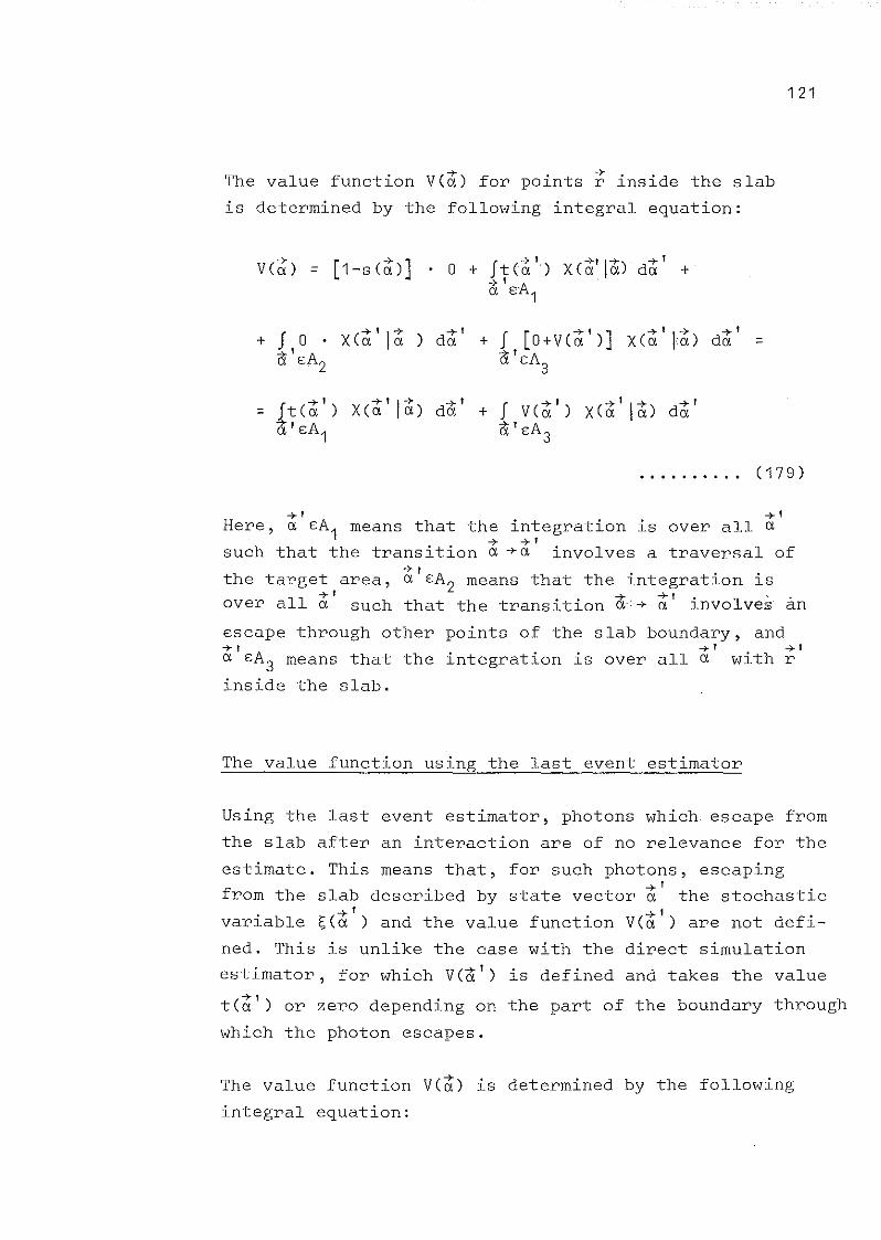
121
The value function vet) for points ~ inside the slab
is determined by the following integral equation:
f .-+-' -+'1+) +'. O + t Ca .) X(a a da ++'a 81\1
+ f O •iY;'8A
2
=
-+' -+11+ +'= lt(a ) XCa a) da +a'8A1
f +'V(a )iY;'8A 3
+'1+ +'XCa a) da
.......... (179)
-+t -+1Here, a 8A1 means that the integration is over all a
+ +'such that the transition a +a involves a traversal of
the target area, ~'8A2 means that the integration is-+t •. -+ -+,. .','
over all a such that the transltlon a<+ CJ. lnvolveq an
escape through other+,a 8A3 means that the
inside the slab.
points of the slab boundary, and-+' -+ I
integration is over all a with r
The value function uSlng the last event estimator
Using the last event estimator, photons which escape from
the slab after an interaction are of no relevance for the
estimate. This means that, for such photons, escaping,from the slab described by state vector ~ the stochastic
variable ~(~') and the value function VC~') are not defi
ned. This is unlike the case with the direct simulation
estimator, for which VCa') is defined and takes the value
tC~') or zero depending on the part of the boundary through
which the photon escapes.
The value function vct) is determined by the following
integral equation:

+= q(a)+T(a)+q(a)
122
-+ -t-, -+'1+ +'= T(a) + J V(a ) X(a a) daa' E:A3
.......... (180)
Using the absorption estimator, the expressions in eq
180 are valid, provided that [1-s(t)] is substituted+forq(a).
The value function using the collision density estimator
As with the last event estimator, the value function is
not defined for photons escaping from the slab after an
interaction. The value function vet) for points ~ inside
the slab is determined by the following integral equation:
vet)+ + J[TCt) V(t' )J X(&:' I&:) dt'= q(a) T (a) + + =
a' E:A3+ + + I X(t' It)
,Sv (t' ) +' + +'
= q(a) T(a) + T(a) da + X(a la) da.+' a' E:Aa E:A3 3
.......... ( 181)
However, since:
+' -+ +' -+JX(a la) da = 1-q(a)'&:' E:A
3
it follows that:
+ J -+' -+'1+ +'= T(a) + V(a) X(a a) da'&:'E:A 3
.......... (182)
.......... (183)
The integral equations 180 and 183 are identical.
123
The last event estimator and the collision density
estimator can also be used to estimate the parameter
(18l+)..........
TAT . The value functions are then given by eqs 180
and 183 with fT(;i). dA substituted for T(;i). However,AT
-+' -+' -+ +'dA = ft(a ) X(a la) da
a' EA1
so that in this case all the integral equations for
the value function are identical. This is a reasonable
result. The contribution to the field quantity T from
a particular interaction in the slab and its successors
is independent of any estimator. While the stochastic
variable ~(;i) depends on the estimator, its expectation
value does not, so long as the estimate is unbiased.
The relation between the field quantity T and the value
function
From the definition of V(;i), it follows that, alterna
tively to the expression in eq l+1, T can be written:
.......... (185 )
The integration in eq 185 is
lies inside the slab.
..,. ..,.over all a such that r
The integral equations for the collision density and
for the value function are usually called adjoint to
each other. The field quantity T can be evaluated by
solving one of them and using either eq l+1 or eq 185.

124
Proof of the expressian for, using the value lunation
The proof of eq 185 can be demonstrated as follows.
The expression for
in the integral on
J ->- ->-F
1(a) V(a) =
->-V(a), eqs
the right
180 and 183, is substituted
hand side of eq 185:
.......... (186)
If the order of integration is revers ed in the double
integral, one finds:
->- I [ -+ '- 1 ---'- -+] ~ I= JV(a )JF1(a) X(~ I~)da d~ =
.......... (187)
If the expression for V(~), eqs 180 and 183, is sub
stituted in eq 187, etc., then one finally derives:
J ->- ->- ->-F 1 (a) V ( a ) da =
J-+ -+ -+ -+ , -+ 1 -+ , .. -+" +If -+"= F1 (a) T(a) dC!, + JF 2 (a ) T(a ) da + JF3(a ) T(C!, ) dC!, +... =
00
= E JF (~) T(~) d~ = JF(~) T(~) d~ = ,n=1 n
.......... (188)

125
3. The value function as importance function
Using the direct simulation estimator and the last
event estimator, the value function is an ideal impor
tance function, which leads to a value of zero for
the variance. Using the collision density estimator, it
is neither possible to prove that the value function is
the best importance function nor that it is possible to
find an importance function which gives a value of zero
for the variance. However, if the value function is used
as an importance function, i.e., if:
+V(a)= , (189)
it can be shown that V(,*) < , using the collision den
sitY estimator (Coveyou et colI 1967).
The direct simulation estimator
Using the importance function:
(190)
the variance, V[(TAT)*], takes a value of zero. The weight
WNassigned to state vector aN of a random walk in which
the transition aN-1 + aN involves traversal of the tar
get area is then given by:
1 .......... (191)
If this is substituted for the weight WN in eq 12~, it
is found that the variance of the estimate becomes zero.
126
It was pointed out earlier that, using the direct simu
lation estimator, a necessary condition for zero variance
is that photons are not allowed to escape from the slab
except through the target area. It can easily be demon
strated that, using the value function as importance
function, this condition real ly is fulfilled. The value
function V(~) takes a value of zero when ~ describes a
photon which escapes from the slab through other parts+
of the boundary than the target area. Then I(a) takes a
value of zero, eq 190, as does finally the fictitious
transition probability density X(~I~'), eq 173 . In the
same way it can be shown that the second necessary condi
tion for zero variance, viz., the condition that photons
are not allowed to be absorbed, is fulfilled.
The last event estimator
Seleeting the importance function according to eq 189
the weight WN associated with state vector ~N(;N within
the slab) takes the value:
1 = T .......... (192 )
Substituting this in eq 1~5 gives:
... .... . .. (193 )
where the integrations in eq .193 are taken over all in~
teraction sequences which lie as a whole within the slab.

127
Now, from eq 180 it follows that:
1 =+T(a)+V (eJ.)
v(ci' )
V(ci)+' 1+ +'X(a a)da "
...... +' -+ +f+ fxcC( 1C()da
+, Aa E: 3. . ... ... . . ( 194 )
and hence that:
.......... ( 195 )
where qCciN) is the fictitious probability that a photon
which interacts described by t N has its last interaction
in the slab.
Substituting q(ciN,WN) from eq 195 in eq 193 then
gives V(T*) " O.
Using the absorption estimator, eqA + .
ded that 1-s(aN,WN) is substltuted
this case, the condition for getting
to zero is obviously that:
193 is valid provi-A +
for q(aN,WN). In
a variance equal
.......... (196)
Then, however, from eq 194 it follows that:
.......... (197)
i.e., in order to get a zero variance using the absorption
estimator photons are not allowed to escape from the slab.

128
Compapison between the absopption and the last event
estimatops undep conditions of zepo vapiance
To get a variance equal to zero the optimal fictitiousA '+
transition probability densities XC~ la) are identical
using the last event and the absorption estimators.
However, when selecting appropriate fictitious frequency
functions for scattering angle and free path before the
next interaction, there is greater freedom using the
last event estimator than when the absorption estimator
is used. In the latter case, there exists the additional
requirement that photons are not allowed to escape from
the slab. Combining
A + + +s Ca) = 1 - TCa)/VCa) witha.e.
Pcn')JA 1+' +1fCp= r -r )O
dJ!; , = 1
where PCn') is the distance from point; to the boundary
of the slab in the direction n', means that the fictitious
frequency function for the scattering angle and the energy
of the scattered photon is uniquely determined from:
,Z::'r**' ,~C~I,~t ) ,hv l / ; =
dChv)d(l1
+ +1-TCa)/VCa)
pcn' )Jxc~' I~)O
+'dr
(198)
Using the last event estimator, however, the photons are
allowed to escape from the slab. This means that the sur
vival probability can be chosen as ~C~) = 1 - TC~)/VC~) + ~C~)
with the escape probability ect) being a number larger than
zero. In turn, this means that there is a freedom in choo
sing the frequency function for the scattering angle and
the energy of the scattered photon. Depending on this choice
the free path frequency function is given by:

f(p
129
A. -+' -+X (a I~a.:...) -:-- """""",,"
[1-T("t)/V("t)+~(t)] [~[(n,til ),hv'l /~]achv) an
.......... (199)
Here, the only requirement on the frequency function for
the scattering angle and the energy of the scattered pho
ton is that for all n':
+'dr < 1 .. .. . .. ... (200)
For intance, if the frequency function for the scattering
angle takes on too low a value for same direction n', this
requirement, eq 200, may be violated.
From eq 199 can be seen that the shape of the free path
frequency function is uniquely determined by the ~'-depen
dence of the transition probability density functionA +' \+ A +X(u a). The choices of the value for e(u) and the frequency
function for the scattering angle only determine a normali
zation of the free path frequency functions as to allow
the scattered photons to escape from the slab with certainA +
probabilities. A given net probability of escape, e(u),
after an interaction described by "t can be obtained by com
bining different frequency functions for the scattering
angle with different probabilities of escape for the pho
tons scattered in different directions (ti,ti'). If, in par
ticular, the frequency function for the scattering angle
is chosen to be identical to that, eq 198, valid for getting
zero variance using the absorption estimator, then each
scattered photon has a probability of escaping which is in
dependent of the particular direction (n,n') of scatter and
is given by the quotient ~(ii)l[~ ("t) + ~("t)].a.e.
Using the direct simulation and the last.event estimatQrg
i t is thus possible, in principle, to find fictitious tram;ition
probability densities such that the variance in the estimate

130
is zero. However, this requires a knowledge of the value-7
function V(a) and to determine this is as difficult as
solving the initial problem. It is thus unreasonable to
consider determining the value function exactly: however,
even an approximate knowledge of it may be very useful.
This can be derived by finding an approximate solution of
the integral equation for the value function, e.g. using
Monte Carlo methods, or by intelligent quessing. In the
latter case, physical insight should be of considerable
use, which is one thing that favours the specialist in
radiation physics in dealing with this topic.
4. Derivation of the exponential transformation of the
free path freguency function using an approximate value
function as importance function
Consider once again a plane radiation shield of thickness
d which is being irradiated homogeneously. The photon
fluence is a function of the depth, z, only. The plane
fluence at the rear of the shield, i.e., for z = d, is
to be determined using the direct simulation estimator.
The function t(~') in eq 179 is then given by t(~') = 1.
The photon fluence can roughly be anticipated to decrease
exponentially with the depth, z, in the shield, with an
unknown "attenuation coefficient", c. If, in eq ,179 , the
'"contribution to the value function V(~) from the second
integral in the last line is neglected, the following
approximate value function V(~) is obtained:
( 201)
If this approximate value function is used as an impor
tance function, the fictitious transition probability den
sities will be given by:

131
=
-c(d-z )n+1e
e
.......... (202)
Substituting in eq202 the relation between zn and zn+1
given in eq 77 gives:
cPn+1cos8n+1e .......... (203)
The altering of the true transition probability density
to give the fictitious one can be looked upon as a change
of the free path frequency function. Normalizing this
such that:
OOA
Jf(p) dp = 1O
gives:
f(p) = (wccos6) e-(Il-Ccos6)p
(204)
. . . . . . . . .. (205)
This free path frequency function is identical to that
which was derived from the exponential transformation of
the transport equation.
B. Splitting methods
1. Splitting of primary photons
With the estimators described above unbiased estimates
are obtained from a single random walk. Usually, how
ever, a number, H, of random walks is used to find esti
mates with smaller variances. Using, for instance, the

132
collision density estimator, the estimate can be written:
1 H= - l:
H h=1.......... (206)
This equation can now be rewritten so that:
H= E
h=1
w:t:l
fr+hT(a, )
l• • • • • • • • •• ( 2O7 )
The factor 1/H can be considered to be included in the
weights W:t:. A primary photon is thus considered to bel
split into H parts, each one of which, h, is given an, , , l ' h ph 1/ A ' b d ' llnltla welg t NO = H. n estlmate ase on a slng e
random walk is then no longer unbiased: this is obtained
first when the estimate is based on H random walks.
The splitting of the primary photon into H parts can be
made in an arbitrary manner. The parts need not neces
sarily be equal, with w~ = 1/H, as assumed above. In
addition, for each part, h, transition probability den
sities can be defined which depend on h.
Now, H random walks are to be generated, one for each
part, h, using the transition probability densities
h ' h h Id f h ' d' 'd l A ' ~***W lC o or eac ln lVl ua part. n estlmate, T
of the field quantity T is evaluated from:
H= E
h=1.......... (208)
with the weights defined by:
w:t:l
.......... (209)

133
Ah -+ -+ ."+ -+.F Cai , ... ,a1 ) may be zero although FCai , ... ,a1 ) lS non-
zero. This means that no interaction sequences t1
, ••• ,tiwill be generated in cases when the fictitious probabi
litY and frequency functions are used for generating ran
dom walks. Weights Wi are then not defined.
The conditions for which this estimate is unbiased will
now be investigated.
. . A***The stochastlc varlable, can be treated as a sum of
stochastic variables ~h* which are themselves in turnAh*sums of stochastic variables ,.
l
H= l:
h=1
00
lii=1
.. .. .. • ... C21 O)
Ah*where the ,. are analogue to the stochastic variables* l'i defined above, page 59.
Th . E[~***] , .e expectatlon value" can then be wrltten as:
H 00
E n***] = l: l: E [~J;*] =h=1 i=1 l
where:
00 Hl: l: E[~J;*li=1 h=1 l
....... (211)
E [~~*] = f ... f
.......... C212)
The integration in eq .212 is over all interaction se
quences which lie as a whole within the slab and are suchAh -+ -+
that F (ai , ... ,a1 ) is nonzero.

134
The estimate is unbiased provided that:
Hl:h=1
(213)
f " -+-+or all lnteractlon sequences u1 , ... ,u i such that
r(~i""'~1) and T(~i) are nonzero, since then:
both
Hl:h=1
H= l:
h=1J... J
= J... J -+ [HT(u,) l:l h=1
-+ -+du i ····· .du1 =
= J... J
J -+ -+-+= T (Ci,,) F. (Os . ) do: .l l l l
Substituting eq 214 in eq 211 gives:
.......... (214)
00
= l: JT(~) ri(~)d~ =i=1
J-+ -+-+
T(u) r(u)du = T .......... (215)
A***i.e., T is an unbiased estimate of T.
Ah -7- -7-Eq 213 implies that r (ui , ... ,u1 ) can, for some parts,
h, but not for all of them at once, be zero even if
(-+ -+ ) , "r u i , ... ,u1 lS nonzero. One partlcular case wlll now be
examined in more detail, viz., the case in which for every-+f h'hr(-+)' Arh1(;t) , f lu or w lC 1 u lS nonzero, ~ lS nonzero or on y
one of the h,

135
Systematic sampling
For every state vector ~ such that F1(~) is nonzero theh +values F1 (a) are all assumed equal to zero except for
one part, h. In addition, for all parts, h, and all
weights w~ the fictitious transition probability den-l
sitY lS assumed to be nonzero as soon as the correspon-
ding true transition probability density is nonzero and
transitions to points within the slab are concerned.
Then:
H A
L: E [T~*] =h=1 l
HL:h=1
H h= L: J... JWoh=1
.......... (216)
Here, every integral in the sum is defined and gets contri-• •• -+-+-
butlons only from those lnteractlon sequences a 1 , ... ,a iAh +for which the F
1(a 1 ) are different from zero. It follows
from this and from the assumptions above that the estimate
is unbiased, provided:
.......... (217)
for all parts h.
In the particular case of a pencil beam, systematic samp
ling implies the following (see Fig 9):

136
d
- ---
Fig 9: The slab lS divided into H layers each of thick
ness ~d. The first interaction of each part, h,
of the splitted primary photon takes place in
one of the layers ~d and only one part interacts
in any particular layer.
For each part h of the primary photon F~(~) is different
from zero only for points ;h with their z-coordinates in
the h:th layer ~d of the slab. If, in addition, the pho
ton is prevented from escaping from the slab without in
teracting, then:
Ah -+ -+JF1 (a)da = 1
f;E:6d
For instance, F~(~) can be selected:
• . . • . • . • •• (218)
.......... (219)
With F~(~) as given by eq .219, one finds for the weighthW1 :
.. • .. • ... (22 O)
where zh denotes the z-coordinate for the position of
the first interaction process for part h.
137
The method of splitting pvimavy photons has been illus-
tvated heve using the collision density estimatov. The
conclusions ave, howevev, genevally tvue independent of
the type of estimatov used. Systematic sampling is, how
evev, of pavticular interest in connection with the colli
sion density estimator fov the following reason.
If the division of the slab into H layevs is made suffi
ciently fine the quantity:
Hl:h=1
H= l:
h=1•.•.••.••• (221)
is appvoximately equal to the field quantity ,(1) for pho
tons which have been scattered once, i.e., with systema
tic sampling and the collision density estimatov, an
approximate analytical calculation of the contribution
to , from photons scatteved once is automatically obtained
If systematic sampling is used in conjunction with the
other estimatovs discussed heve, the contribution to ,
from photons scattered once is obtained stochastically
and not analytically.
Of couvse, with slight modifications, it is possible to
use all estimatovs for estimating the field quantity of
multiply scattered photons only and then in all cases to
add the analytically calculated contvibution from photons
which have been scatteved once.
Does systematic sampling veduce the variance? When the
primary photon is split into H pavts, H random walks
are needed before an unbiased estimate ~*** is obtained.
It should thevefore be. . "***ln estlmate ,
veasonable to compare the variance. . . ft** . h .wlth that ln an estlmate, ,WhlC lS
ft*the avevaged value of Hestimates , using unsplit primary
h t . ft**. l IP o ons, Slnce, lS also based on H random wa ks. n
addition, it should be veasonable that, in such a compa
rison, the transition probability densities used in gene-
138
rating random walks should be the same in all cases. In
systematic sampling, it is possible to consider using
different fictitious transition probability densities
for the h different parts of the primary photon. But,
what form shall be assumed for the frequency function
for the free path prior to the first interaction in
evaluating T*? The variance in the estimate ~* is cer
tainly dependent on this free path frequency function.
Even if all transition probability densities and the
frequency function for the free path prior to the first
interaction are taken to be the analogue ones, it is
difficult to prove anything or to make any statement
which is general ly valid.
However, when systematic sampling is used in conjunction
with the collision density estimator, an approximately
analytical determination of the contribution to T from
photons scattered once is obtained and this suggests
that the variance in the estimate will be reduced, par
ticularly at points for which the relative contribution
from such photons is large.
With the aim of decreasing the variance, systematic samp
ling can be extended in the following manner. If it is
known that the largest contribution to the variance in, A*** h' h ' f' ,the estlmate T comes from p otons Wlt thelr lrst ln-
teractions in a particular layer, sampling can be concen
trated to these photons, e.g., by generating more random
walks for them. An unbiased estimate, ~****, can then
be formed from:
A****T .......... (222)
where Nh is the number of photons with their first inter
action in layer h. Provided that Nh is chosen to be lar
gest for those layers, h, which give the largest contri-
b , h' , A*** h . A****.ut lons to t e varlance ln T ,t e estlmate T lS,
as regards the variance, more favourable than a.. . A*** Th'forward arlthmetlc mean of estlmates , . lS
139
straight
is an
example of a so called stratified sampling scheme.
Tt is warth painting out a particular advantage of using
systematic sampling in connection with estimating the field
quantity , behind slabs of different thicknesses. Some
parts of random walks generated with a thick slab can be
used when making estimates for thinner slabs: as saon as
arandom walk generates a state vector with its position
coordinate outside the thinner slab, it is finished as far
as the latter is concerned. The state vectors of arandom
walk generated with a thick slab can, however, up to this
point also be used in estimating , at the rear of the thin
ner slab. On the other hand, a disadvantage of the methad
is that the fictitious transition probability densities
cannot be chosen in relation to the thickness of the slab,
i.e., they cannot be optimized for each and every single
thickness.
Comments on estimating the variance in estimates using
systematic sampling
Th h t , . b Ah* , he stoc as lC varla les, are lndependent of one anot er,
but have different expectation values as weIl as different
variances depending on the particular layer h. The H values. Ah*obtained for the different stochastic varlables, cannot
be looked upon as samples for the same stachastic variable.
An expression equivalent to that in eq 108 for estimating
V[T***] from the H random walks generated cannot be used.
A***An unbiased estimate, S2, of Ve, 1 can, however, be
obtained if the experiment of generating H random walks
is repeated M times and:

1M-i
Ml.:m=1
H[l.:
h=1
h,mT -
1 M- l.:M m=1
Hl.:h=1
· .
140
(223)
h mwhere T 'Ah*T at the
is the value taken
m:th experiment.
by the stochastic variable
2. Splitting of photons along random walks
A photon described by state vector ~ associated withn
weight Wn can just prior to or after an interaction be
split into H pieces, each assigned a weight Wh such that:n
H= l.:
h=1· " (224)
Usually, the choice Wh = W IH is made. Forn na continuation of the random walk, denoted
+h o o o··,aN lS generated. The welghts asslgnedh
vectors are given by:
every part h,+h +h
by a n +1 , Cln +1 , .•
to these state
= w~l A ~ -+ '
X(ao+1!CJ,o ,Wo)l l l
l ). n · . . . . . . . .. ( 225 )
An unbiased estimate of T is obtained by summing contri
butions from the random walks of the individual parts,
e.g., when using the direct simulation estimator:
H= l.:
h=1(226)
+hwhere t(aN )o hdlS travers e
is replaced by zero unIess the target area
by the escaping photon.

1l+ 1
Using the last event estimator,
H= 1:
h=1
+hTCuN )b ••••••••• , C2 27)
and, using the collison density estimator,
n= 1:
i=1
+W.TCu. )
l l
H+ 1:
h=1
h +hW.TCu.) .......... (228)l l
+hwhere uNh
by photon
describes the last interaction in the slab
part h.
Proof that these estimates are unbiased is left to the
reader.
Further splittings along the random walks can be made
and unbiased estimates obtained by summing over the to
tal number of random walks created.
When using this splitting method, it is not usual to work
with fictitious transition probability densities but in
stead to generate random walks by analogue simulation.
Used in combination with Russian roulette of survival
the method is in fact an alternative to importance samp
ling using fictitious transition probability densities.
The importance function then provides the tool to deter
mine both when photons should be split up and the number
of parts into which they should be decomposed. If a pho-+ . +
ton goes from a state un to a more lmportant state, un +1 '
a splitting of the photon in the ratio ICtn +1
)/ICtn
) is
made. In case this quotient is not an integer, the photon
is with probability q' split into q+1 pieces and with pro
bability 1-q' split into q pieces where q is the integral
part of the quotient ICt 1)/ICt) and q' is its fractionaln+ n

part. The photon is then on the average split into+ +q'(q+1) + (1-q') q = q + q' = I(un +1 )/I(un ) pieces.
If, on the other hand, the transition is to a less im-+ .
portant state, un +1 , the random walk lS terminated at
~n+1 with probability 1-I(~n+1)/I(~n)'
As pointed out above, the important regions in ~-space
are those giving the largest contributions to the variance
in the estimate using analogue simulation. Using splitting
as described above the variance is reduced by increasing+the sampling in important regions of u-space and decrea-
sing it in less important regions just as in importance
sampling using fictitious transition probability densi
ties. When the photon splitting method is used, more effort
has to be spent in generating random walks than is needed
using fictitious transition probability densities. On the
other hand, no effort has to be spent in determining appro
priate . fictitious transtition probability densities so
that random walks are more rapidly generated.
C. Correlated sampling
When investigating the effect of using different sets of
interaction cross sections on the results of Monte Carlo
calculations, the use of correlated sampling is often to
be recommended, particularly when the differences in the
cross sections are small. The procedure is as follows.
Arandom walk [~1 ""~NJ is generated using a particular
frequency function F1 (d) and a particular set of transi
tion probability densities X(~'I~). From this random walk
two estimates ~~ and ~; are made. For instance, using the
collision density estimator, the estimates are given by:

143
A*N 2 ->-
'2 = l: W. T(o. i )i=1 l
where
->- ->-
W:F1 (o. i ,···,o.1 )
=l A ->- ->-F(o.
i, ... ,0.
1)
and
->- ->-2 F 2 (o. i ,···,o.1 )
w. =l A ->- ->-F(o. i ,· .. ,0.1 )
.......... (229)
......... , (230)
.......... (231)
.......... (232)
(->- ->- ->- ->- ) ••
Here, F1 o. i , ... ,o.1 ) and F2 (o. i , ... ,o.1 are the probablllty
densities for interacting via the sequence t 1 , ... ,t i accor
ding to two different sets of interaction cross sections.
F(ti , ... ,t1
) is the corresponding probability density de-r. -+ A -+' -+
fined by F1
(o.) and X(o. 10.) used in generating the random
walk. The value of T(t.) is calculated appropriate to thel
set 1 or 2 of interaction cross sections considered, cf.,
eqs 42 - 45.
When the transport process is defined by set 1 of cross
sections the field quantity , takes the value 'i while
it takes the value '2 when the transport process is de-"* A*fined by set 2 of cross sections. Now, 'i and '2 in eqs
229 and 230 are unbiased estimates of 'i and '2 pro-A(->- ->- ) • (->- ) •vided that F o. i , ... ,o.
1lS nonzero as soon as T o. i lS
• -+ -+ -+-+nonzero together wlth both F
1(a. i , ... ,a.
1) and F
2(o. i , ... ,o.1 )
and theinteraction sequence is within the slab.
In generating random walks,
to correspond to one of the
A -+- A +' -+F
1(a.) and X(o. 10.) may be chosen
sets 1 and 2 of cross sections

144
considered in the investigation. However, the set chosen
for this must permit all transitions possible with the
other set of cross sections. For instance, assume that
a comparison is to be made between using an interaction
model in which atomic electrons are free and at rest at
the moment of interaction and a more realistic one taking
account of the binding energies of such electrons. With
bound electrons, photons may be scattered without losing
energy which is obviously not possible for photons scat
tered against free electrons. In generating random walks
there must ,exist a nonzero probability that photons areA -T A. -+' -+-
scattered without energy loss. F1 (a) and ~(a ja) must in
this case be chosen to correspond to the set of the cross
sections found from the model considering bound electrons.
A comparison of the results from two different calcula
tions can be presented as either the difference or the
quotient between the values obtained.
If theA*
and '2
A*difference between the stochastic variables '1
is investigated, then:
(233)
...•••••.• (234)
"* A~ A* A *with C('1"2) the covariance of '1 and '2'
If, on the other hand, the
h t · . bl A* *C as lC varla es '1 and '2
quotient between the
is regarded, then:
two sto-
= .......... (235)

1TT:) 2
2
145
2(T 1 )TT)4·
2
. . . . . . . . .. (236)
The relations in eqs 235 and 236 follow from Gauss's
approximation formula. They are thus approximations and
as such must be used with some caution. In particular,A~ A~
it must be realized that T1
/T 2 is only approximately an
unbiased estimate of the ratio T1
/T 2' For the approxima
tion to be reasonable, it is necessary that at least ~;
does not take value close to zero. In using, e.g. the
direct simulation estimator, it is not at all uncommonA* . .for T 2 to take the value zero. However, by formlng estl-
"** A**mates T1 and T 2 based on a number of random walks rather
than on just one, this difficulty can be avoided.
• ,,;tE ...... *The covariance of two stochastic varlables T1 and T 2 can
k o.. If All' d All'ta e posltlve, negatlve and zero values. T 1 an T 2are independent stochastic variables, the covariance is
zero. In particular, if estimates ~~ and ~; are based on
different independent random walks, ~~ and T; are indepen
dent of each other.
In this case, two advantages are attained when the cova
riance is positive. The variance is reduced in comparisonA* A*to its value when C(T
1,T 2 ) is equal to zero, c.f. eq 234
In addition, computing time is saved by using one and the"* A*same random walk for evalueating both T
1and T 2 .
A* "*The covariance of T1 and T 2 is given by the expression:
00
= l:N=1
NJoo.J[l:
i=1
N[l:i=1
(237)
146
In eq 237 , the covariance is the one valid using the
collision density estimator. This does not in any way
limit the generality of what follows. A positive corre
lation, i.e. a positive covariance, is obtained whenA* A* .'1 and '2 tend for every random walk to devlate in the
same direction from their expectation values '1 and '2'
In particular, if F1(~N""'~1) does not differ great ly+ + l 2
from F2 (aN, .. . ,a1 ) then Wi ~ Wi "1 ~ '2 and the cova-
riance can be expected to be positive and close to
V[~~] ~ V[~~] such that the variance in eq , 234 will be
very close tö zero. In this case it should be worthwhile
to use correlated sampling.
In the expressions for the variances in the differenceA* A* A* A*
and the quotient between '1 and '2' V['11 and V['2J areth . f A* d A* . h .e varlances o '1 an '2 Wlt respect to that partlcu-
lar set of transition probability densities which is used
in generating the random walks on which both ~~artd ~~ areA* A*
based. For noncorrelated estimates '1 and '2' i.e., when
the estimates are based on different random walks, there
is the possibility of generating these using different
transition probability densities. The values for V[T~J and
V[T~] are then not identical to those in eq 233 and it
need in fact not be the case that the variance in the dif-. A* A*.
ference or the quotlent between '1 and '2 wlll be less if
correlated sampling is used, even if the covariance is po
sitive. However, if the difference in the sets of cross
sections used is small, then the difference in the opti
mal variance reducing fictitious transition probability
densities will also be small and the positive correlation
so strong that the use of correlated sampling must be pre
ferred.
Details of correlated sampling when used together with
the direct simulation estimator
As has already been point ed out the frequency function
147
Fi(~) and the transition probability densities X(~' I~)
used in generating random walks may be chosen identical
to those defined by one of the sets of interaction cross
sections being investigated.
_A * _A *When estimates (T
iAT ) and (T 2AT ) are made using the
direct simulation estimator, it can be shown that if ran-. -+ +' 1+ .dom walks are generated uSlng F i (a) and x1 (a a) and lf_ _ _ * _A *
T 2AT ) Ti
AT > O then the covariance of (Ti
AT ) and (T 2AT )
is always positive. Even if T2AT < Ti AT , positive values
for the covariance can be obtained. It is only necessary
that the difference between the expectation values is suf
ficiently small.
To prove the above statements, the following relation for
the covariance of two stochastic variables T~ and T; forms
a convenient starting point:
(238 )
Using
value
the direct simulation estimator, the expectation_A * _A *
of the product between (Ti
AT ) and (T2
AT
) is
given by:
(239 )
The integrations in eq 239 are made over all interaction+ +sequences a
i, ... ,aN which end with traversal of the tar-
get area AT' Note that the values taken by the weight
function t(~) are not dependent on the values on any
cross sections, contrary to the values taken by the
148
weight function T(&) used with the last event and the
collision density estimators.
A + + + +Furthermore, if F(a
N, ... ,a
1) is put equal to F1 (aN, ... ,a1 )
then:
. • . • • • • • •• (240)
and the covariance is glven by:
.......... (241)
It follows immediately that the covariance lS positive
when T2AT ~ Ti AT > O.
If, on the other hand O < T2
AT < T1
AT , then there exists
a positive number s such that:
.......... (242)
I
In addition, there exists another positive number s such
that:
.......... (243)

1'49
From eq 241 , it now follows that the covariance is
positive if c'< c, i.e., if the difference between the
expectation values T1AT and T2AT is sufficiently small.I
If, however, E > E, then the covariance becomes nega-
tive and correlated sampling can in this case not be
recommended, cf, eq 234.
D. Linear combinations of estimators
An unbiased
combination
A*estimate T of T can be obtained as a linearA *of unbiased estimates T
X
x= ~ k T*
x=1 x x.......... (244)
Provided that E[~*] is equal to T for all x and the sumx A*
of all kx
is equal to one, T is an unbiased estimate
of T.
A*Now, T may simply be equal to the average of X esti-
mates of T based on X different random walks using one
and the same estimator. Then k = i/X and ~* is identi-A** . x .
cal to the estimates T dlscussed above wlth X = H. In
this case the lowest value for the variance in ~*
tained with k = i/X = i/H.x
is ob-
A linear combination of unbiased estimates ~* can alsox
be obtained by generating one random walk and making
X estimates of T using different estimators. For simp
licity, consider X = 2. Then:
A*and the variance, VeT ), is given by:
........... (245)
(246)

150
A* "')jE.Now, especially if the covariance of T 1 and T 2 lS nega-
All'tive the variance in T may be considerably less than
A* A* A* A*both V(T 1 ) and V(T 2 ) when the estimates T1 and T2 are
based on one single random walk.
All'depends on the covariance of T
1and
for c. The minimum value of
All'The variance V(T )A*T 2 but also on the value
( A*). b .V T lS otalned when:
c =
Linear combinations of estimates using different esti
mators can thus be exploited as a varlance reducing
method (Spanier and Gelbard, Halperin).
It has been shown that, using importance sampling with
the aid of importance functions, it is possible to re
duce the variance in estimates to zero. This ideal situa
tion is, however, not practically achievable so that the
method of using linear combinations of different estima
tors sketched here may weIl be worthwhile using.
A l . A* A* b' d .s an examp e, conslder that T1
and T2
are o talne uSlng
the last event and the collision density estimators re-. l Th . f A* d A*. . bspectlve y. en the covarlance o T
1an T
2lS glven y:
N .,.T] [J.: W.T(o:.) - T]F(tN'''''~1). 1 l ll=
(248 )

151
Roughly speaking, a negative value for the covariance
is obtained if WNTC~N)/qC~N,WN) tends to take large
values when LWiTC~i) takes small values and vice versa,
such that the integrands in the sum of eq 248 predo
minantly take on negative values.
E. Antithetic variates
Pairs of strongly negatively correlated stochastic varia
bles form the base for the variance reducing method of
antithetic variates.
Consider the following example: in the pencil beam slab
penetration problem, the position at the first interaction
is chosen from a free path frequency function f Cp). Assume
that this is normalized in the interval [O,d] i.e., that
no source photons escape without interacting in the slab.
Now, the position at the first interaction is selected
by selecting arandom number p. Then C1-p) determines
another position for the first interaction. Starting from
these two positions for the first interaction, two random
lk d . . * d *wa s are generate lndependently and estlmates T 1 an T 2of T, using the same estimator, are made bas ed on these
two random walks. Then:
* + /\ ~~1 T2=
2
(249)
A* A*is an unbiased estimate of T provided that both T 1 and T 2are unbiased estimates of T.
glven by:
(250)

152
A* A*. A*If C(T1 ,T2 ) is negatlve, then the variance V(T ) is
less than the variance in an estimate bas ed on two non
correlated random walks. In the latter case the varianceA*is equal to V(T
1)/2.
In this example, it cannot be proved but only anticipatedA* A* .that the stochastic variables T
1and T2 are negatlvely cor-
related. Other pairs of presumably negatively correlated
stochastic variables may be found depending on the parti
cular problem to be solved.
Here, only a simple application of the method of antithe
tic variates has been discussed. The general development
of this method was first made by Hammersley and Morton
1956.
III. Results of some methodological investigations con
cerning the simulation of photon transport through a
water slab.
In a test study of importance sampling, seven different
programmes for calculating the plane fluence at diffe
rent points on the rear of a water slab irradiated with
a perpendicularly incident pencil beam of primary pho
tons have been evaluated.
One of the programmes used the collision density esti
mator, while in the others the direct simulation estima
tor was employed.
The water slab has been assumed to be 15 cm thick and the
incident photons to have an energy distribution correspon
ding to a 70 kV bremsstrahlung spectrum. A 70 kV energy
spectrum has been chosen to permit comparison with the re
sults of Monte Carlo calculations carried out by REISS
and STEINLE. In addition, it has been assumed that all
scattering processes are Compton processes with free elec-

153
trons at rest, i.e., scattering is described by the
Klein-Nishina cross sections. The effect of taking
into account the binding energies of the atomic elec
trons has been investigated separately using correla
ted sampling, cf., L Kusoffsky 1975 b.
In estimating with the collision density estimator
fictitious probability and frequency functions have been
used throughout. These have been seleeted as follows:
1. The free path prior to the first interaction has been
seleeted from a rectangular frequency function:
A 1-1f(p) = 15 cm .......... (251)
This free path frequency function is such that the pro
bability of a primary photon passing through the water
without interacting is zero.
2. Analytical averaging of survival has been used in con
junction with Russian roulette, in the form given in
eq 158 .
3. The angle of scattering has been taken to be distribu
ted isotropically, i.e., the frequency function for
the scattering angle has been taken to be of the form
given in eq ,169 .. The energies of scattered photons
are given by the Compton relation, eq 17 .
4. The free path between interactions has been seleeted
using a free path frequency function as given in eq
163 with:
C2 52)
In estimating with the direct simulation estimator, ana
logue simulation has been used throughout as has nonana-

154
logue simulation according to the scheme described above.
In addition, different combinations of some of these fic
titious probability and frequency functions and analogue
ones have been used.
Using the direct simulation estimator, the rear surface
of the slab was divided into a number of target areas as
follows: a circle of radius 1 cm, its centre coinciding
with the exit point of the primary pencil beam, was se
lected 'and the area was then, up to a distance 14 cm from
the centre, divided into annular rings of width 1 cm. All
point s lying more than 14 cm from the centre were consi
dered to comprise a single target area.
To limit the range of possible values of the estimates
using the collision density estimator, finite target areas
were again used. This was carried out by placing a circle
1 cm in diameter symmetrically around the exit point of
the primary beam. At distances corresponding to even va
lues of centimetres Cup to 14 cm) from the centre defined
by the exit point, eight circular target areas each of
area 1 cm2 were placed symmetrically in a ring about the
centre. For each random walk an estimate of the plane
fluence was made for each of these target areas and the
average of the eight values was final ly used as an esti
mate of the plane fluence at the distance of the ring
from the centre. This procedure is such that the cylind
rical symmetry inherent in the problem has also been uti
lized in estimating with the collision density estimator.
Using the collision density estimator, the final estimate
was based on 3000 random walks while, using any one of
the direct simulation estimators, the corresponding num
ber of random walks was 100 000. The camputing time
for making an estimate was then about the same in each of
the seven programmes.
In each program using the collision density estimator, the

1 . The cylindrical symmetry of
target areas ln the form of
The increase ln the size of
155
plane fluence, T, was, as described above, estimated for
points at 15, and using the direct simulation estimators
at 14, different distances equidistant 1 cm from the centre.
As a measure of the precision of a program, the average
of the relative standard deviations (as determined from
experimental data) in the estimates at the different dis
tances from the centre was used. In none of the cases did
these relative standard deviations differ with more than
a factor of two - with a tendency for them to increase
with increasing distance from the centre.
No significant difference in precision among the various
programmes could be demonstrated. The relative standard
deviation varied between 7% and 9% and the computing cost
between 50 and 80 units.
Since only 3 000 random walks were generated using the
collision density estimator against the 100 000 using any
one of the direct simulation estimators, it is apparent
that the precision per random walk is larger using the
collision density estimator. That the overall efficiency
is no better is due to the fact that more time is needed->-
to calculate a value for ~W.T(a.) than to calculate a val l
lue for WNt(uN) using the direct simulation estimators.
These cbmparisons seems to point to the conclusion that
it is not really worthwhile to use the more complicated
procedures involved in the collision density estimator.
However, it must not be forgotten that, ln this special
geometry, a direct simulation estimator is favoured be
cause of two factors:
the problem is such that
annular rings can be used.
the target area with increa-
sing distance from the centre then compensates for the
corresponding decrease in the plane fluence. The re la-

156
tive standard deviation in estimates at different distan
ces from the centre thus remains relatively constant,
even rather far out. The relative standard deviation in
estimates using the collision density estimator does
not depend on the effect of a target area which increa
ses with increasing distance from the centre. In the
absence of cylindrical symmetry, the collision density
estimator would probably be preferable.
2. The number of target areas does not great ly influence
the computing time (cost) in programmes based on the
direct simulation estimator, whereas in programmes using
the collision density estimator, the computing time in
creases about linearly with the number of target areas.
This is the case since calculating LW.T(~.) for a tar-l l
get area takes about as much time as generating a ran-
dom walk. If, for instance, only the value of the plane
fluence at one particular distance from the centre is
of interest, the computing time would be reduced to
about 1/15 using the collision density estimator, but
would not be much altered using the direct simulation
estimator.
An advantage of the direct simulation estimator is that,
at very little extra cost, the total number of photons
transmitted through the slab can be estimated. When this
number is required, it is not easy to determine it using
the collision density estimator. On the other hand, a
programme using the collision density estimator can easily
be supplemented with a programme in which the direct si
mulation estimator is utilized to estimate the total num
ber of photons passing outside the central circle inside
which the plane fluence is estimated using the collision
density estimator. The same set of random walks can beused with the direct simulation estimator to estimate the
number of these photons as is used to estimate the plane
fluence at points inside the circle with the collision
density estimator.
157
Using the collision density estimator, photons can be pre
vented from escaping from the slab, whereas, using the
direct simulation estimator, this is possible only for
photons which escape through other points than those of
the target area. An analytically modified direct simula
tion estimator can then be used to supplement a programme
making use of the collision density estimator and in which
photons are prevented from escaping from the slab. This
estimator is described in the Appendix.
A programme has also been developed to test the use of sys
tematic sampling in conjunction with the collision density
estimator. The water slab was divided into 3 000 layers.
Each estimate of the plane fluence was thus based on 3 000
random walks to make comparisons with the corresponding
estimates described above using the collision density esti
mator reasonable. The same fictitious probability and fre
quency functions have been used in both programmes.
The use of systematic sampling resulted in improved pre
cision in the estimate of the plane fluence averaged over
the central target area, consisting of the circle 1 cm in
diameter centered at the exit point of the primary photons.
There, the relative contribution to the plane fluence from
photons scattered once is largest and this contribution is
calculated analytically using systematic sampling in con
junction with the collision density estimator. On the other
hand, at points rather far away from the center the experi
mentally determined relative standard deviation in the es
timate was occasionally considerably larger using systema
tic sampling. This could be traced to the occurrence in
the experimental data of few very large values for the
plane fluence. When the collision density estimator is
used, the value taken by the estimate can be very large,
for instance, when the position coordinate of a state vec
tor Ceollision point) in arandom walk is elose to the
target area. The frequency function for the estimate ~*
is in faet very skew so that s2 is a bad measure of the
158
varianee. If the number of random walks on whieh the es
timate s2 of the varianee is bas ed is small the probabi
litY that a high value for i* is obtained is also small
and s2 tends to underestimate the varianee. Now, the es
timate s2 of the varianee in an estimate using systema
tie sampling has to be based on a number, m, of repeti
tions of the program, ef., eq223 . Here, m was ehosen
to be ten so that, in all, ten times 3 000 random walks
were generated. Thus, there was more ehanee of getting
a eollision point elose to any partieular target area
than in the ease in whieh the 3 000 random walks on whieh
the estimate of the plane fluenee was based were also
used for estimating the varianee.
Leaving the above differenees out of aeeount, the program
using systematie sampling was found to have the same effi
eieney as the one without systematie sampling. The reason
for this may be found in the partieular fietitious rrequeney
function for the free path before the first interaetion,
eq 251, whieh was used in the latter ease. With this free
path frequeney funetion the points at whieh the first in
teraetions oeeur will be fairly evenly distributed aeross
the slab. In systematie sampling an even distribution of
these points aeross the slab is made deterministieally.
It must be emphasized that the investigations deseribed
here only have the eharaeter of pilot ones. No systema
tie investigations to optimize the fietitious probabi
lity and frequeney funetions have been made. There is
also eertainly mueh whieh ean be done to reduee eompu
ting time and henee running eosts. However, despite this,
the investigations reported here should be able to pro
vide some indieation of the possibilities and limitations
of the different methods.
As is usually the ease, the work with the partieular pro
jeet referred to here, was first started on a more or
less intuitive basis, the more thorough analysis of avail-

159
able methods being made later. The last event estimator
was noticed only towards the end and has thus not been
investigated in practical calculations. This estimator
is of interest since there is the possibility of finding
a zero value of the variance in the estimate, which is
not the case using the collision density estimator. On
the whole, the last event estimator should share some
of the advantages (and even the disadvantages) of the
collision density estimator not to be found using the
direct simulation estimator. Furthermore, it should be
worthwhile to try alternative variance reducing methods
such as linear combinations of estimators and antithetic
variates.

160
APPENDIX
An analytically modified direct simulation estimator
Arandom walk [t1, ... ,tNl is generated and an estimate- *(TAT ) of the parameter TAT is made according to:
Here,
N-i= L
i=1
N= L
i=1
in cases when the random
walk ends with absorption+
at r N and
ln cases when the random
walk ends with the photon
escaping from the slab
+r(cy,,)
l= t(+ ) -~(hV'+1)P(0'+1)a i +1 e l l (253)
if ni +1 point s through the target area. Then p(ni +1 ) is
the distance from ~. to the target area in the directionlni +1 . If ni +1 does not point through the target area
r(ti ) is equal to zero. The weight function t(t) is iden
tical to that used in conjunction with the direct simu
lation estimator.
The proof that this estimator yields an unbiased estimate
of the parameter TAT is left to the reader. The fundamen
tal relation on which this proof rests is that given in
eq 181+ .

161References
1. G Blom: Sannolikhetsteori och statistikteori med tillämpningar.Studentlitteratur. Lund 1970.
2. L L Carter and E D CashweIl: Particle-transport simulationwith the Monte Carlo method. ERDA Critical Review Series.USERDA Technical Information Center, Oak Ridge, Tennessee.October 1975.
3. R R Coveyou, V R Cain and K J Yost: Adjoint and importancein Monte Carlo application. Nucl Sci Engng 11 (1967), 219-234.
4. U Fano, L V Spencer and M J Berger: Penetration and diffusionof X-rays. Handbuch der Physik. Band 38/2, 660-817.Ed by S Flligge, Springer Verlag 1959.
5. M Halperin: Almost linearly-optimum combination of unbiasedestimates. J Am Stat Assoc ~ (1961), 36-43.
6. J M H~rsley and K W Morton: A new Monte Carlo technique:Antithetic variates. Proc Camb Phil Soc 22 (1956), 449.
7. J M Hamme~sley and D C Handscomb: Monte Carlo methods. Methuenand Co Ltd, London (1964).
8. H Kahn: Random sampling (Monte Carlo) techniques in neutronattenuation problems - I. Nucleonics ~ (1950), 27-37.
9. H KalIi: On the variance reduction techniques in Monte Carlosolutions of neutron transport problems. Acta PolytechnicaScandinavica. Physics including nucleonics series No 89.Helsinki 1972.
10. L Kusoffsky: Rutinbeskrivningar. Monte Carlo program för fotontransportsimuleringar. LiU-RAD-R-029; 1975 a.
11. L Kusoffsky: Jämförelse mellan två olika växelverkansmodellerför 15-200 keV fotoner använda i Monte Carlo beräkningar avspridd strålning. LiU-RAD-R-030- 1975 b.
12. M Leimdörfer: A Monte Carlo method for the analysis of gammaradiation transport from distributed sources in laminatedshields. Nucleonik, 6. Band, 2. Heft (1964), 58-65.
13. M Leimdörfer: On the transformation of the transport equationfor solving deep penetration problems by the Monte Carlo method.Chalmers tekniska högskolas handlingar. Nr 286, 1964.
14. K H Reiss, B Steinle: Tabellen zur Röntgendiagnostik,Siemens AG, DB med, Erlangen 1973.
15. J Spanier and E M Gelbard: Monte Carlo principles and neutrontransport problems. Addison-Wesley Publishing Company.London 1969.
16. W Vesely: A study of the effects of polarization, electronbinding, and Rayleigh scattering in Monte Carlo gamma ray transport calculations. Ph D Thesis University of Illinois (1968).