effect of urbanization on the thermal structure in the … of urbanization on the thermal structure...

Effect of Urbanization on the Thermal Structure

in the Atmosphere

by R. VISKANTA, R. 0 . JOHNSON, and R. W. BERGSTROM, JR., School of Mechanical Engineering, Purdue University, West Lafay- ette, Ind. 47907. The senior author is professor of mechanical engineering; Johnson is a graduate assistant, now with the Division of Engineering Design., Tennessee Valley Authority, Knoxville, Tenn. 37902; and Bergstrom is a postdoctoral fellow, now a research associate at NASA Ames Research Center, Moffett Field, Calif. 94035.

ABSTRACT.-An unsteady two-dimensional transport model was used to study the short-term effects of urbanization and air pollution on the thermal structure in the urban atmosphere. A number of simulations for summer conditions representing the city of St. Louis were performed. The diurnal variation of the surface temperature and thermal structure are presented and the influences of various parameters are discussed.

IT IS ESSENTIAL in air-pollution forecasting to understand how urban-

ization and the urban area modify the atmospheric environment not only in the immediate vicinity of the city, but also for a considerable distance downwind. Modification of the environment takes on many forms and includes alteration of the wind, temperature, and water- vapor proflles a s well a s t he surface temperature and the injection of gaseous and particulate pollutants into the atmosphere.

During the past few years, many serious atempts have been made to ob- serve and explain the microclimatic effects over and around urban areas. The best-documented and least-questioned climatic effect is the urban influence on temperature in the atmosphere. The urban heat-island phenomena is clearly a result of the modification of surface and atmospheric parameters by urbanization, which in t u r n leads to a n altered energy balance. The possible causes of the heat island a re well recognized (Peterson 1 9 6 9 ) , but the individual effects such a s physical and radiative property differences between urban and rural areas, flow changes caused by the roughness elements, man-made heat

sources and radiatively participating pollutants have not been sufficiently studied, and their quantitative influences a re not completely understood.

Observational programs and mathematical modeling a re needed to gain understanding of t he urban environment. Unfortunately, the very nature of the urban environment necessitates extensive measurements over large dis- tances and long periods of time, which a r e not only difficult but also costly. Therefore mathematical models can be employed to advantage to help fill the observational gap by numerically simu- lating the transport processes in the atmosphere. To the extent tha t the niathematical model simulates the real atmosphere, i t can then become a valu- able tool for use in micrometeorological weather prediction, forcasting of pollution episodes, urban planning, inter- pretation of field data, and identification of pollutants by means of remote sens- ing methods.

In addition to the above, numerical simulations can also be used a s a guide for observational programs such a s the Regional Air Pollution Study (RAPS) sponsored by the U. S. Environmental Protection Agency ( E P A ) for the St.

Louis Metropolitan area. The main advantage of a numerical simulation lies in its ability to predict what will happen for any given changes in urban parameters, boundary, or initial conditions.

In this paper we will describe the short-term effects of urbanization on the thermal structure in the atmosphere of an urban area, using an unsteady two- dimensional transport model. The em- phasis is on the potential effects of urbanization and a i r pollution on the thermal structure in the urban planetary boundary layer. As a specific example, results of numerical simulations of the city of St. Louis for summer conditions a re discussed. Results of similar experiments have been reported (Pnndolfo et n2. 1971, Atzvuter 1972, Bornstein 1972, Wagner and Yu 1972, and Atzoater 1974) .

NUMERICAL MODEL Physical Model and Assumptions

In the unsteady two-dimensional transport model (fig. I ) , the earth- atmosphere system is assumed to be composed of four layers : (1) the free

(natural) atmosphere where the meteorological variables a re considered to be time-independent ; (2) the polluted atmosphere (the planetary boundary layer, PBL) , where the meteorological variables such as the horizontal, vertical, and lateral wind velocities, temperature, water vapor, and pollutant concentrations a re functions of time, height, and distance along the urban area; (3) the soil layer, where the temperature is assumed to be a function of deptli and time only (the soil and interfacial radiation lsroperties are allowed to vary in the horizontal direction) ; and (4) the lithosphere, where the temperature is assumed to be constant during the simulation period. The atmosphere is assumed to be cloud-free, and no variation of topogralshy is accounted for along the urban area.

In the polluted urban planetary boundary layer the transport of momentum, energy, and species takes place by vertical and horizontal advection as well as by vertical and horizontal turbulent diffusion. In addition, radiative energy is transported in the solar (short-wave)

Figure I .-Schematic representation of the urban environment and of influences analyzed by the urban boundary layer model.

u, v, 8, p, C,, C,, C, SPECIFIED

FREE I ATMOSPHERE

ATMOSPHERE

I I

PLANETARY

and thermal (long-wave) portions of the spectrum. The interaction of both natural atmospheric constituents and gaseous as well as particulate pollutants with solar and thermal radiation is accounted for. The planetary boundary layer and soil layer are coupled by energy and species balances a t the atmosphere-soil interface. The horizontal variation of the urban parameters such as man-made heat and pollutant sources, surface solar albedo (reflectance) and thermal emittance, surface roughness, thermal diffusivity and conductivity of the soil, and Halstead's soil moisture parameter are arbitrarily prescribed functions of position along the urban area. I t has been observed (Stern et nl. 1972) that the man-made heat and pollutant sources, for example, vary during the diurnal cycle. However, more real- istic modeling of these sources during the diurnal cycle must await more com- plete observational data.

Model Equations The numerical model is based on the

conservation equations of mass, momentum, energy, and species. The equations used to describe the planetary boundary layer can be written in a general form as

where t, x, and z are the time, horizontal, and vertical coordinates ; u and w a re the horizontal and vertical velocity components ; +i (x,z,t) is the dependent variable "conserved ;" Si (x,z,t) is the appropriate source term; and KXi and K,i are suitable turbulent diffusivities. The independent variables and their corres- ponding sources a re listed in table 1. A general discussion of the conservation equations was given by Plate (1971), and Johnson (1 975) presented a detailed derivation of the equations used in the model.

The boundary conditions prescribed a t the edge of the outer flow (top of the PBL) and a t the soil surface a re the following : a t the edge of the outer flow, +i is specified ; a t the interface, u = v = w = 0 ; and the surface temperature (a t any x) is predicted from an energy balance

, - P I

a+i a+i a+i a ( 2) In this equation, the first two terms -+u-f W-=-- K,i- at ax az ax account for absorption of solar and

thermal radiation, the third term repre- sents thermal emission, the fourth and fifth terms account for sensible and latent heat transfer by molecular and

[I] turbulent diffusion, the sixth term rep-

Table I .-Dependent variables and source terms

1 u horizontal velocity f (v-v,) geostrophic deviation

2 v lateral velocity f (ug-U) geostrophic deviation

3 fj potential temperature aF/az, q radiative and man-made heat sources

4 C, water-vapor concentration C , water vapor emission

5 C i concentration of pollutant aerosol CI pollution emission

6 C2 concentration of gaseous pollutant cz pollution emission

resents heat conduction into the ground, and the final term is the man-made surface heat flux. The water vapor concentration a t the surface is prescribed by Halstead's moisture parameter (Pnn- dolfo e t (11. 1971) by the expression

c , (x,O) =M(x) Cw,sat[T(x,O) I + [I-M (x) IC, (ZIP) [31

where M is the moisture parameter, Cw,s,t is the water-vapor concentration a t saturated conditions, and z, is the first grid point above the surface. For a prescribed pollutant flux a t the surface, m,,, a species balance a t the interface, yields the condition

ployed for the prediction of the diffusivities in the transition layer under stable conditions.

Stable conditions were assumed to exist when the average Richardson number in the lowest 25 m of the atmosphere was greater than zero. Where this condition was reached, Pandolfo's model was used only near the surface, while the polynomial was employed in the transition layer. Otherwise, Pandolfo's model was used throughout the entire PBL. If the Richardson number ex- ceeded the critical value, i t was reset to this value so that unreasonable diffusivity values would not be predicted.

At the upwind boundary, the meteorological variables are predicted from the unsteady one-dimensional model of Berg- strom and Viskanta (1973a). Initially, +i is specified everywhere and is assumed to be independent of the horizontal coordinate x.

Turbulent Diffusivities Specification of turbulent diffusivities

for an urban atmosphere in connection with numerical modeling of the PBL is a very difficult task and has been discussed in a recent review (Oke 1973n). The semi-empirical equations developed by Pandolfo et al. (1971 ) were initially employed. The decay of turbulence in the upper part of the PBL was prescribed by following Blackadar's (1962) formulation. However, in the hours before sunrise, when the atmosphere be- came quite stable, unrealistically deep surface inversions resulted and the Richardson numbers were found to ex- ceed the critical value.

In these situations the diffusivities predicted by Pandolfo's eddy diffusivity- Richardson number correlations were not applicable. Therefore, the cubic polynomial developed by O'Brien (1970) and used by Bornstein (1972) was em-

Radiative Transfer Model The radiative transfer model used has

been discussed in detail elsewhere (Bergstrom and Visknntn 1973b), so only a summary of i t is included here. The urban atmosphere is considered to be cloudless, plane-parallel, and consist- ing of two layers: (1) the free atmosphere, and (2) the urban PBL where the pollutants are concentrated. The earth's surface was considered to emit and reflect radiation as prescribed functions of wavelength. Since the atmospheric gases and particles absorb, emit, and scatter radiation, the radiative transfer between the free atmosphere and the PBL is coupled. However, no consideration is given to individual point sources of pollutants. Since multidimen- sional radiative transfer is complex, i t is assumed that the transport of radiation can be approximated by a quasi- two-dimensional field based on the vertical temperature, water-vapor, and pollutant distributions a t several pre- determined horizontal positions. The radiative fluxes in the atmosphere are then evaluated a t a few prescribed horizontal locations and linear or non- linear interpolation is then used to de- termine the radiative fluxes between these locations.

The radiative fluxes and flux diver- gences are evaluated by dividing the

entire electromagnetic spectrum into solar (0.3 < A < 4 pm) and thermal (4 < A < 100 pm) portions. The computational details can be found in Berg- strom and Viskanta (1973h). Total emissivity data for water vapor and car- bon dioxide were used, and scattering was neglected in predicting radiative transfer in the thermal part of the spectrum. I t was assumed that the influence of gaseous pollutants could be confined to the 8 to 12 pm spectral region due to the relative opacity of the H,O and CO, bands. Ethylene or sulfur dioxide were considered to be representative pollutants. The spectral absorption and scattering characteristics of the aerosol in a polluted atmosphere were taken from the model developed by Bergstrom (1 972 ) .

Numerical Method of Solution The alternating - direction - implicit

(ADI) method (Ronche 1972) was employed to solve the transport equations [ I ] . The selection of suitable grid spacing, appropriate finite-diff erence ap- proximations for the spatial derivatives and the algorithm itself, and tests for convergence a re discussed in detail by Johnson (1 975) . To improve the resolu- tion near the surface, a logarithmic- uniform grid spacing was chosen in the vertical direction. The logarithmic spacing extended to about 1 km from the earth surface, and from there to the top of the PBL (- 2 km) the spacing was uniform. A uniform spacing was also

employed in the horizontal direction and in the soil layer.

The number of grid points and their spacing in the vertical and horizontal directions can be varied. The results reported have been obtained by using 22 nodes in the vertical direction and 17 in the horizontal direction. The first vertical grid point was located a t 5 m from the surface and the horizontal grid spacing was 1.5 km. The program required practically the entire high-speed memory capacity (138,000/150,000 bytes octal) of the National Center for Atmospheric Research CDC-7600 digital computer. The computational time was approxi- mately 8 minutes for a 24-hour simulation period.

RESULTS AND DISCUSSION

Numerical Experiments The numerical model has been tested,

and a number of numerical experiments have been performed, using the city of St. Louis as an example. Because of the length and scope of the paper, i t is possible to include only some selected results for the temperature in the atmosphere. The experiments were de- signed to simulate the thermal structure and pollutant dispersion in the urban atmosphere. The urban area was mod- eled by varying the appropriate surface parameters between rural and urban values in the horizontal direction. The value of these interface parameters are given in table 2. A horizontal distribu-

Table 2.-Numerical values of interface parameters for simulations (Johnson, 1975)

Parameter Upwind Urban ru ra l Center

Solar albedo 0.18 0.12 Thermal emittance .90 .95 Soil thermal conductivity (W/mK) .1 .5 Soil thermal diffusivity (107 m2/s) 1 2.5 Surface roughness (m) .2 1.0 Moisture availability parameter .1 .05 Lower soil boundary temperature ( K ) 295.5 295.5 Urban heat source (W/m2) 2 20 Aerosol pollutant source ( r g / m 2 ~ ) 0 2.5 or 5 Pollutant gas source (ug/m2s) 0 2.5 or 5

tion was established by selecting the values of parameters a t the rural and urban center locations and, for lack of any better data or information, a Gaus- sian distribution curve was then fitted between the urban and rural locations by specifying the standard deviation of a suitably chosen mean value. The data given in table 2 are representative values over the city.

The simulations were started a t 1200 solar time and continued for a 24-hour period. The initial temperature profiles used were taken from Lettau and David- son (1957) for 24 August 1954 and were imposed over the entire area (no x- variation). The initial horizontal and lateral velocity fields were either identical to or decreased by a factor of 2 of

those given by Lettau and Davidson for the O'Neill Great Plains Turbulence Study. The pollutant-concentration profiles were initialized to a constant back- ground value of 50 pg/m3.

Components of the Energy Budget at the Surface

The surface temperature can be considered as the forcing function of the model. Thus i t is important to understand the variation of the energy budget components along the urban area. These are presented in figures 2 and 3 a t 2400 of the first day and 1200 of the second day. Inspection of figure 2 shows that the emitted (q,.) and the absorbed thermal (q,,) fluxes are the dominant components. The turbulent (q,), the latent

Figure 2.-Variation of the surface balance flux components (qt-turbulent, q,-latent, q,-emitted, q,s-absorbed solar, qat-absorbed thermal, q,-ground conduction, Q-urban heat source) a t the surface a t 2400 of the first day; Gaussian distribution, radiatively nonparticipating, u,=6 m/s and v,=4 m/s.

400

P

7 qe

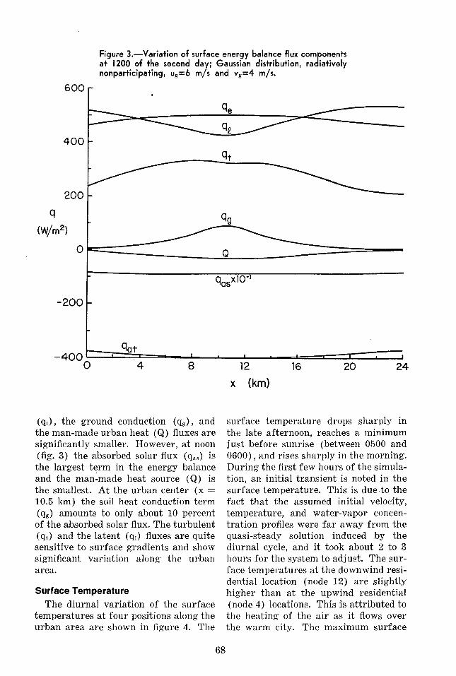
Figure 3.-Variation o f surface energy balance flux corn onents a+ 1200 of the second day: Gaussian distribution, raJatively nonparticipating, u,=6 rn/s and v,=4 rnJs.

r

(q,) , the ground conduction (q,), and the man-made urban heat (Q) fluxes a re significantly smaller. However, a t noon (fig. 3) the absorbed solar flux (q,,,) is the largest term in the energy balance and the man-made heat source (Q) is the smallest. At the urban center (x = 10.5 km) the soil heat conduction term (q,) amounts to only about 10 percent of the absorbed solar flux. The turbulent (q,) and the latent (q,) fluxes a re quite sensitive to surface gradients and show significant variation along the urban area.

Surface Temperature The diurnal variation of the surface

temperatures a t four positions along the urban area are shown in figure 4. The

surface temperature drops sharply in the late afternoon, reaches a minimum just before sunrise (between 0500 and 0600), and rises sharply in the morning. During the first few hours of the simulation, an initial transient is noted in the surface temperature. This is due to the fact that the assumed initial velocity, temperature, and water-vapor concentration profiles were f a r away from the quasi-steady solution induced by the diurnal cycle, and i t took about 2 to 3 hours for the system to adjust. The surface temperatures a t the downwind residential location (node 12) are slightly higher than a t the upwind residential (node 4) locations. This is attributed to the heating of the a i r as i t flows over the warm city. The maximum surface

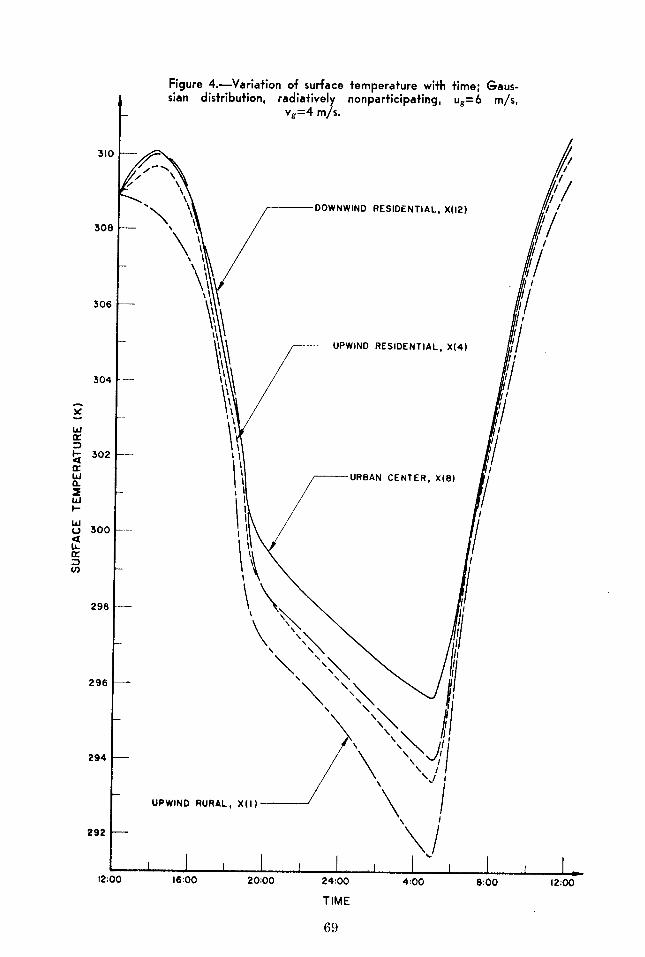
temperature difference (about 4OC) between the urban center and upwind rural locations occurs just before sunrise. On the other hand, for a simulation with higher wind speeds (u, = 12 m/s and v, = 8 m/s) , the maximum difference occurs in the evening a t 1900 and re- mains almost constant throughout the night ( J o h n s o n 1975).

The effect of radiatively participating pollutants as measured by a local surface-temperature difference (temperature with participating pollutants/temperature without) is illustrated in figure 5. The temperature differences result from an interaction between many complex phenomena, and therefore individual influences a re not easily identified. The surface temperature difference is largest during the night and reaches a maximum before sunrise 0500 and is smallest a t noon. The differences be-

tween the surface temperatures a re con- siderably smaller for higher wind speeds ( J o h n s o n 1.975).

A comparison of the surface temperatures for the Gaussian and rectangular distributions of urban man-made heat sources is illustrated in figure 6. The results show that the difference between the two results is only about 1°C, and the maximum occurs early in the morning (0500) when the man-made urban heat source is a significant component of the energy budget. At noon (1200) the surface temperatures in the city differ by only about O.l°C, indicating the predominance of the radiant energy transfer in the interfacial energy balance.

Temperature Structure The isopleths of the two-dimensional

potential temperature fields a t 6-hour

Figure 5.-Local surface temperature difference (simulation with radiatively participating ollutants minus simulation with P radiatively nonparticipating po lutants) along the city; Gaussian distribution, ethylene (C2H4)-pollutant gas, u,=6 m/s, v,=4 m/s, m, =m2=2.5 pg/m2s.

Figure 6.-Comparison of surface temperatures for Gaussian and rectangular distributions of urban heat and pollutant sources; radiatively participating, ethylene (CzH4)-pollutant gas, u p 6 m/s, v,=4 m/s, ml=mz=2.5 pg/mZs.

---- RECTANGULAR GAUSSIAN

intervals for a simulation with radiatively nonparticipating pollutants are shown in figure 7. At 1800 the atmosphere is nearly adiabatic, especially in the upwind rural area, with a thermal plume having a temperature of about 305 K forming a t a height of about 100 n~ downwind of the city center (node 8, x = 10.5 km). Note that the last digit denoting the temperature of the iso- therm a t 1800, 2400, and 0600 hours has been truncated. However, the plume is not felt downwind, and the upwind and downwind surface temperatures a re nearly identical. A surface temperature inversion develops a t night and is seen to be deeper over the rural area than over the city. This is indicative of the nocturnal heat island, which decreases the stability of the atmosphere. The magnitude of this heat island is larger a t night than during the day. This tjrpe of behavior is well documented (Petrr-

son 1969, Oke 1973b) . Just after sunrise (0600) the breakup of the stable layer was noted. The surface inversion breaks up rapidly after sunrise due to heating of the surface by absorption of solar radiation, and by 0900 all traces of the inversion have disappeared. Simi- lar types of diurnal variation of thermal structure have been found for other simulations under different conditions (Johnson 1975) .

The maximum temperature difference between simulations with radiatively participating and nonparticipatng pollutants occurs a t the urban center late a t night (fig. 8 ) . The temperature differences are seen to be largest near the surface and a re confined to the lowest 600 meters of the PBL. When the pollutant gas is assumed to have the radiative properties of sulfuy dioxide (SO,), the temperature structure predicted is practically the same as that for the

Figure 7.-lsopleths of potential temperature (in K); Gaussian distribution, radiatively nonparticipating, u p 6 m/s, v,=4 m/s.

0 6 12 18 0 6 12 18 24 x (km)

(a) t = 18:OO (b) t = 24:OO

Figure 8.-Comparison of thermodynamic temperatures at the urban center; Gaussian distribution, ethylene (C2H4)-pollutant gas, u p 6 m/s, v,=4 m/s, ml=m2=2.5 pg/mzs.

NONPARTICIPATING ------ PARTICIPATING

- E ' 400 -

200 - t=18:00

radiatively nonparticipating pollutant gas. This is due to the fact that SO1 is a weakly radiating gas. The results are consistent with those obtained with the one-dimensional model (Bergstrom and Viskr~nta 1973n). The net effect of the city and the human activity on the temperature distribution is illustrated in figure 9. The results show that the presence of radatively participating pollutants dampens the amplitude of the diurnal temperature variations and that for a relatively short (24-hour) simulation the effects a re confined primarily below 600 m.

Urban Heat Island The urban heat island is a well-known

and accepted fact (Peterson 1969, Oke 1973b). The urban heat-island itensity (maximum difference between upwind rural and highest urban surface temperature, at,-,) predicted is shown in figure 10. For the assumed Gaussian distribution of man-made heat sources, the maximum surface temperature difference occurred a t the urban center,

whereas for the rectangular distribution during the night i t occurred downwind of the center. The results presented in the figure show that there is a double peak in AT,,-,.. The first peak is noted a t about 2000. I t arises due to the more rapid cooling a t the upwind rural area than in the city. The maximum heat- island intensity occurs just before sunrise and has a magnitude of about 4OC. For the population of the urban area and wind speeds of the simulation this value is in good agreement with the observations and empirical correlation of Oke (1973b). For a simulation with lower wind speeds (u, -- 2.4 m/s and v, -- 1.6 m/s) , which are not reported here, the maximum heat-island intensity reached about 10°C. This is also in good agreement with the nighttime and day- time observed temperature excesses between the urban and rural locations (Oke 1973b, DeMarrais 1975).

CONCLUSIONS As a result of a limited number of

numerical simulations that have been

Figure 9.-Comparison of perturbation potential temperatures (temperature in the cit minus the temperature at the upwind rural location) at the ur r, an center for radiatively nonparticipating (a) and radiatively participating (b) simulations; Gaussian distribution, ethylene (C2H,)-pollutant gas, u p 6 m/s, v,=4 m/s, ml=m2=2.5 pg/m2s.

@' (to 63' (to

Figure 10.-Comparison of maximum urban upwind rural surface temperature differences; ethylene (C,H,)-pollutant gas, ug=6 m/s, vg=4 m/s, ml=m2=2.5 rg/m2s.

NONPARTICIPATING ------ PARTICIPATING A

" 12:OO 16:OO 20:OO 24:OO 04:OO 08:OO 12:OO

TIME

perforn~ed for selected meteorological LITERATURE CITED conditions during the summer, the fol- Atwater, Marshall A.

1972. THERMAL CHANGES INDUCED BY URBAN- lowing generalizations can be made : IZATION. Am. Meteorol. Soc. Conf. on Urban

Environ. and 2d Conf. on Biometeorol.: 1. The unsteady two-dimensional trans- 153-158. Boston.

port model predicts an urban heat- A t ; $ a 7 ~ r k ~ ~ ~ ~ ~ 1 d " , . A N G E S INDUCED BY POLLu- island intensity that is sensitive to TANTS FOR DIFFERENT CLIMATIC REGIONS. Am. wind speed and latent energy trans- Meteorol. Soc. Symp. on Atmos. Diffusion

and Air Pollut. : 147-150. Boston. port through Halstead's moisture Rergstrom, Robert W., Jr.

~h~ intensity of the ur- 1972. PREDICTIONS OF THE SPECTRAL ABSORP- TION AND EXTINCTION COEFFICIENTS OF A N

ban heat island reached a magnitude URBAN AIR POLLUTION AEROSOL MODEL. Atmos. of about 4OC near sunrise and about be^^^^^^; ~ o ~ : ~ ~ 2 & 8 ; Jr., and 1.4OC a t noon. Raymond Viskanta.

2. F~~ the conditions the radia- 1973a. MODELING THE EFFECTS OF GASEOUS AND PARTICULATE POLLUTANTS IN THE URBAN

tively participating pollutants are ATMOSPHERE. PART I. THERMAL STRUCTURE. J. Appl. Meteorol. 12 : 901-913. in Rergstrom, R. W., Jr., and K. Viskanta.

the urban heat island compared to 1973b. PREDICTION OF THE SOLAR RADIANT

other factors. During the night, a i r FLUX AND RATES IN A ATMOSPHERE. Tellus 25 : 486-498.

pollution does increase the surface Blackadar, Alfred K. temperature by about 1 . 2 5 0 ~ at the 1962. THE VERTICAL DISTRIBUTION OF WIND

AND TURBULENT EXCHANGE IN A NEUTRAL urban center. ATMOSPHERE. J. Geophys. Res. 67: 3095-3102.

3. The role of radiatively participating B O ~ & $ ~ $ $ ~ ~ ~ & S I O N A L , NON-STEADY NUM- pollutants in the formation of the ERICAL SIMULATIONS OF NIGHTTIME FLOWS OF

thermal structure is relatively small A STABLE PLANETARY BOUNDARY LAYER OVER A ROUGH WARM CITY. Am. Meteorol. Soc. Conf.

and i t is greatest late a t night. The on Urban Environ. and 2d Conf. on Bio- meteorol. : 89-94. Boston. largest effect of pollutants was to de- DeMarrais, Gerard A.

crease the stability a t night and hence 1975. NOCTURNAL HEAT ISLAND INTENSITIES

increase turbulent transport near the ~ ~ & ~ ~ ~ $ C ~ e ~ ~ h e ~ ~ ~ S ~ ~ 4 :0135ytl.NG surface particularly a t heights below Johnson, Robert 0. 500 m. 1975. THE DEVELOPMENT OF AN UNSTEADY

TWO-DIMENSIONAL TRANSPORT MODEL I N A 4. The feedback mechanism between POLLUTED URBAN ATMOSPHERE. M.S. thesis,

Purdue University. 209 p. ~~~~~~~~~9 structure, Lettau, Heinz H., and Ben Davidson, editors. and dispersion has the potential of 1957. EXPLORING THE ATMOSPHERE'S FIRST

being significant in modifying pol- MILE. VOL. I AND 11. Pergamon Press, New York. 578 p.

lutant concentrations under more O'Brien, James J. stable conditions and higher pollutant 1970. ON THE I'ERTICAL STRUCTURE OF THE

EDDY EXCHANGE COEFFICIENT. J. Atmos. Sci. loadings. However, the magnitudes 27 : 1213-1215.

of the changes a re dependent on the O k ~ i ~ ~ A URBAN

coupling between the radiative prop- 1968-1972. Univ. Brit. Columbia Dep. Geogr., erties of a i r pollution and the buoy- o ~ ~ ~ " " ~ ancy-enhanced turbulence. Due to 197313. CITY SIZE AND URBAN HEAT ISLAND.

Atmos. Environ. 7 : 769-779. the uncertainties in predict- Pandolfo, Joseph P., Marshall A. Atwater, ing either of these two quantities, the and Gerald E. Anderson. magnitude of these changes is un- 1971. PREDICTION BY NUMERICAL MODELS O F

TRANSPORT AND DIFFUSION IN AN URBAN certain. BOUNDARY LAYER. Cent. for Environ. and

Man Final Rep. Hartford, Conn. 139 p. Peterson, James T.

1969. THE CLIMATE OF CITIES: A SURi7EY OF RECENT LITERATURE. Air. Pollut. Control Adm., Publ. AP-59. 48 p. Washington, D. C.

Plate, Erich J. 1971. AERODYNAMIC CHARACTERISTICS O F AT- MOSPHERIC BOUNDARY LAYERS. U.S. Atomic Energy Comm. Div. Tech. Inf. Oak Ridge, Tenn. 190 p.

75

Roache, Patrick J. 1972. COMPUTATIONAL FLUID DYNAMICS. Her- mosa Publishers, Albuquerque, N. M. 434 p.

Stern, Arthur C., Henry C. Wholers, Richard W. Boubel, and William P. Lowry.

1972. FUNDAMENTALS O F AIR POLLUTION. Academic Press, New York. 492 p.

Wagner, Norman K., and Tsann-wang Yu. 1972. HEAT ISLAND FORMATION: A NUMERICAL EXPERIMENT. Am. Meteorol. Soc. Conf. on Urban Environ. and 2d Conf. on Biome- teorol. : 83-88. Boston.

Acknowledgments. This work was sup- ported by the Division of Meteorology, U.S. Environmental Protection Agency, under Grant No. R801102 and R803514. Computer facilities were made available by Purdue University and the National Center for Atmospheric Research. The interest and support of J. T. Peterson, grant project officer, is acknowledged with sincere thanks. The authors also thank A. Venka- tram for his contributions to this effort.

effect of urbanization on the thermal structure in the … of urbanization on the thermal structure...

Documents