effect of soil compressibility in transient seepage
TRANSCRIPT
EFFECT OF SOIL COMPRESSIBILITY IN TRANSIENT SEEPAGE ANALYSES 1
2
3
4
Timothy D. Stark, F.ASCE, D.GE 5
Professor of Civil and Environmental Engineering 6
University of Illinois at Urbana-Champaign 7
205 N. Mathews Ave. 8
Urbana, IL 61801 9
(217) 333-7394 10
333-9464 Fax 11
13
Navid Jafari 14
Graduate Research Assistant of Civil and Environmental Engineering 15
University of Illinois at Urbana-Champaign 16
205 N. Mathews Ave. 17
Urbana, IL 61801 18
20
and 21
22
Aaron Leopold 23
Undergraduate Assistant of Civil and Environmental Engineering 24
University of Illinois at Urbana-Champaign 25
205 N. Mathews Ave. 26
Urbana, IL 61801 27
29
30
31
Paper# GTENG-???? 32
A paper TO BE submitted for review and possible publication in the 33
ASCE Journal of Geotechnical and Geoenvironmental Engineering 34
October 28, 2012 35
36
37
38
39
40
Effect of Soil Compressibility on Transient Seepage Analyses 41
42
Timothy D. Stark1, F.ASCE, D.GE, Navid Jafari
2, S.M., ASCE, and Aaron Leopold
3, S.M.ASCE 43
44
ABSTRACT: 45
Most analyses of levee underseepage, erosion, piping, heave, and sand boil formation are based 46
on steady seepage flow because the computations are simpler and steady-state seepage 47
parameters are less difficult to determine than the corresponding transient parameters, and yield 48
conservative results. However, transient seepage is more representative of levee seepage 49
conditions because the boundary conditions acting on the levee or floodwall change with time, 50
which induces pore-water pressure changes with time in the embankment and foundation strata. 51
In addition, these boundary conditions, e.g., flood surge or storm event, are rapid such that 52
steady state conditions may not have time to develop in the embankment and foundation 53
materials. This paper presents the large and important affects that the coefficient of 54
compressibility, mv, can have on levee and floodwall seepage during flood and hurricane events 55
via a parametric study. This paper also presents methods for evaluating and selecting mv and 56
provides recommendations for performing transient seepage analyses. 57
58
Keywords: transient seepage analysis, hydraulic conductivity, compressibility, levee, gradient 59
60
61
62
63
64
65
66
67
68
69
70
71
72
1 Professor, Dept. of Civil and Environmental Engineering, Univ. of Illinois, 205 N. Mathews Ave., IL 61801-2352.
E-mail: [email protected] 2 Doctoral Candidate, Dept. of Civil and Environmental Engineering, Univ. of Illinois, 205 N. Mathews Ave., IL
61801-2352. E-mail: [email protected] 3 Undergraduate Assistant, Dept. of Civil and Environmental Engineering, Univ. of Illinois, 205 N. Mathews Ave.,
IL 61801-2352. E-mail: [email protected]
INTRODUCTION 73
74
Levees are a significant part of the United States flood protection infrastructure. It is estimated 75
that over 161,000 km (100,000 miles) of levees exist in the United States. The vast majority of 76
the levees across the nation are not part of any federal program. There are approximately 14,800 77
miles of levee enrolled in US Army Corps of Engineers programs (including those built by the 78
Corps and locally maintained) and another 14,000-16,000 miles estimated to be operated by 79
other federal agencies (US Bureau of Reclamation, National Resources Conservation Service). 80
The reliability and performance of levees, e.g., New Orleans and Sacramento-San 81
Joaquin, to hurricane and flood events are based on steady state analyses. Transient seepage 82
analyses are important to evaluate seepage performance of floodwalls and levees because steady 83
state analyses provide a conservative design scenario. The flood or hurricane conditions typically 84
only act for a period of days to weeks, which may not allow sufficient time to develop steady 85
state conditions. As a result, a transient seepage analysis provides a more realistic approach to 86
evaluating levee seepage and stability especially for failure causation analyses. Although a safe 87
levee design may be correctly analyzed using a transient model, a steady state analysis will yield 88
a conservative result. However, a steady state analysis of an existing levee may indicate 89
unsatisfactory performance or an erroneous failure causation mechanism. 90
During a transient levee seepage analysis, e.g., a flood event, pore-water pressures are 91
generated by: (1) partially saturated seepage through the levee and (2) underseepage through 92
pervious foundation strata. The first seepage mechanism involves dissipating the negative 93
(suction) pore-water pressure to positive pore-water pressure as the phreatic surface progresses 94
through the levee. The second mechanism is dependent on the hydraulic conductivity, hydraulic 95
conductivity ratio (kv/kh), and coefficient of volume compressibility (mv) of the foundation strata. 96
The impact of hydraulic conductivity and hydraulic conductivity ratio are widely documented, 97
e.g., Cedergren (1989). This paper presents the large and important affects that mv can have on 98
levee and floodwall seepage during flood and hurricane events. This paper also presents methods 99
for evaluating and selecting mv and provides recommendations for performing transient seepage 100
analyses. Finally, a hypothetical parametric study is presented to show the relationship between 101
pore-water pressure and time to reach steady state condition for a range of hydraulic conductivity 102
and mv values. 103
104
BACKGROUND 105
106
Most analyses of underseepage, erosion, piping, heave, and sand boil formation have been based 107
on steady seepage flow because the computations are simpler and steady-state seepage 108
parameters are less difficult to determine than the corresponding transient parameters. However, 109
transient seepage is more representative of seepage conditions for channel embankments, levees, 110
and floodwalls (Peter 1982). 111
In general, flow is considered to be transient if changes in water level in wells and 112
piezometers are measurable, i.e., hydraulic gradient is changing in a measurable way (Kruseman 113
and Ritter 1991). Freeze and Cherry (1979) state that transient flow (unsteady or nonsteady flow) 114
occurs when at any point in a flow field the magnitude or direction of flow velocity changes with 115
time. In addition, Lambe and Whitman (1969) define transient flow as the condition during fluid 116
flow where pore-water pressure, and thus total head, changes with time. Based on these 117
definitions, transient seepage analyses are applicable to levees and floodwalls because the 118
boundary conditions acting on the levee or floodwall change with time, which induces pore-119
water pressure changes with time in the embankment and foundation strata. More importantly, 120
these boundary conditions, e.g., flood surge or storm event, are rapid such that steady state 121
conditions may not have time to develop. 122
The U.S. Army Corps of Engineers (USACE) design manual for design and construction 123
of levees (2000) details the analysis of underseepage and foundation uplift pressures for levees. 124
The procedure to evaluate the quantity of underseepage, uplift pressures and hydraulic gradients 125
was developed based on closed form solutions to differential equations of seepage flow 126
presented by Bennett (1946). The equations in this Engineer Manual are developed considering 127
a two-layer foundation, which is a typical geological condition in Lower Mississippi River 128
Valley, and steady state conditions. The manual does not require transient seepage analyses for 129
design of levees or floodwalls. Instead, the USACE is currently basing undeerseepage and slope 130
stability analyses on steady state boundary conditions, which can lead to conservative results and 131
results that do not model field conditions. 132
Hydraulic gradient are a function of soil hydraulic conductivity, hydraulic conductivity 133
ratio, i.e., ratio of vertical to horizontal hydraulic conductivity, and mv which is now being 134
included in commercial seepage software. The first two soil characteristics are known to greatly 135
affect transient seepage pore pressure generation. However, the coefficient of volume 136
compressibility is relatively new to commercial software and transient seepage. 137
138
SEEPAGE THEORY 139
140
This section reviews transient seepage theory and provides methods for determining mv. The law 141
of mass conservation for steady state flow through a saturated porous medium requires that the 142
rate of fluid mass flow into any elemental control volume be equal to the rate of fluid mass flow 143
out of the any elemental control volume. The equation of continuity that translates this law into 144
mathematical form is: 145
146
( )
( )
( )
(1)
147
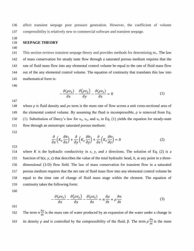
where ρ is fluid density and ρυ term is the mass rate of flow across a unit cross-sectional area of 148
the elemental control volume. By assuming the fluid is incompressible, ρ is removed from Eq. 149
(1). Substitution of Darcy’s law for υx, υy, and υz in Eq. (1) yields the equation for steady-state 150
flow through an anisotropic saturated porous medium: 151
152
(
)
(
)
(
) (2)
153
where K is the hydraulic conductivity in x, y, and z directions. The solution of Eq. (2) is a 154
function of h(x, y, z) that describes the value of the total hydraulic head, h, at any point in a three-155
dimensional (3-D) flow field. The law of mass conservation for transient flow in a saturated 156
porous medium requires that the net rate of fluid mass flow into any elemental control volume be 157
equal to the time rate of change of fluid mass stage within the element. The equation of 158
continuity takes the following form: 159
160
( )
( )
( )
(3)
161
The term
is the mass rate of water produced by an expansion of the water under a change in 162
its density ρ and is controlled by the compressibility of the fluid, β. The term
is the mass 163
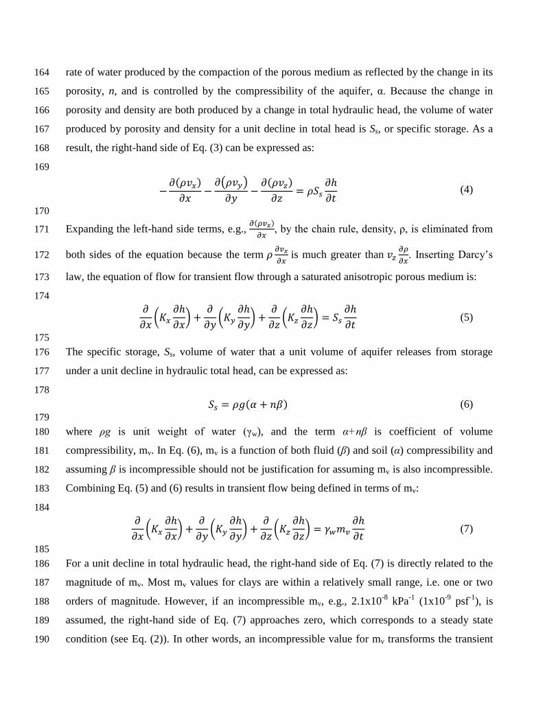
rate of water produced by the compaction of the porous medium as reflected by the change in its 164
porosity, n, and is controlled by the compressibility of the aquifer, α. Because the change in 165
porosity and density are both produced by a change in total hydraulic head, the volume of water 166
produced by porosity and density for a unit decline in total head is Ss, or specific storage. As a 167
result, the right-hand side of Eq. (3) can be expressed as: 168
169
( )
( )
( )
(4)
170
Expanding the left-hand side terms, e.g., ( )
, by the chain rule, density, ρ, is eliminated from 171
both sides of the equation because the term
is much greater than
. Inserting Darcy’s 172
law, the equation of flow for transient flow through a saturated anisotropic porous medium is: 173
174
(
)
(
)
(
)
(5)
175
The specific storage, Ss, volume of water that a unit volume of aquifer releases from storage 176
under a unit decline in hydraulic total head, can be expressed as: 177
178
( ) (6)
179
where ρg is unit weight of water (γw), and the term α+nβ is coefficient of volume 180
compressibility, mv. In Eq. (6), mv is a function of both fluid (β) and soil (α) compressibility and 181
assuming β is incompressible should not be justification for assuming mv is also incompressible. 182
Combining Eq. (5) and (6) results in transient flow being defined in terms of mv: 183
184
(
)
(
)
(
)
(7)
185
For a unit decline in total hydraulic head, the right-hand side of Eq. (7) is directly related to the 186
magnitude of mv. Most mv values for clays are within a relatively small range, i.e. one or two 187
orders of magnitude. However, if an incompressible mv, e.g., 2.1x10⁻⁸
kPa-1
(1x10⁻⁹
psf-1
), is 188
assumed, the right-hand side of Eq. (7) approaches zero, which corresponds to a steady state 189
condition (see Eq. (2)). In other words, an incompressible value for mv transforms the transient 190
flow equation (Eq. (7)) into the steady state flow equation (Eq. (2)). Consequently, the resulting 191
seepage analysis simulates a steady state condition and generates higher pore-water pressures 192
and gradients than observed in the field. 193
194
ESTIMATING SOIL COMPRESSIBILITY 195
196
Coefficient of volume compressibility is the change in volume induced in a material under an 197
applied stress, i.e., the ratio of the change in strain to the resulting change in stress (∆εv/∆σv), or 198
simply the inverse of the modulus of elasticity. The coefficient of volume compressibility is 199
determined from consolidation test data according to: 200
201
(8)
202
where M is the modulus of elasticity in confined compression. From consolidation test data, mv 203
can be expressed in terms of: 204
205
(9)
206
where av is the coefficient of compressibility and eo is the initial void ratio. Finally, mv can be 207
defined in terms of compression index, Cc, and σva, average of initial and final stresses: 208
209
( ) (10)
210
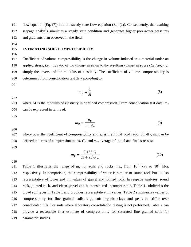
Table 1 illustrates the range of mv for soils and rocks, i.e., from 10-3
kPa to 10-8
kPa, 211
respectively. In comparison, the compressibility of water is similar to sound rock but is also 212
representative of lower end mv values of gravel and jointed rock. In seepage analyses, sound 213
rock, jointed rock, and clean gravel can be considered incompressible. Table 1 subdivides the 214
broad soil types in Table 1 and provides representative mv values. Table 2 summarizes values of 215
compressibility for fine grained soils, e.g., soft organic clays and peats to stiffer over 216
consolidated tills. For soils where laboratory consolidation testing is not performed, Table 2 can 217
provide a reasonable first estimate of compressibility for saturated fine grained soils for 218
parametric studies. 219
220
Table 1: Range of mv values for various materials (after Domenico and Mifflin 1965) 221
222
Soil Type mv (kPa-1
) mv (psf-1
)
Plastic clay 2.1x10⁻³
to 2.6x10⁻⁴
1x10⁻⁴
to 1.25x10⁻⁵
Stiff clay 2.6x10⁻⁴
to 1.3x10⁻⁴
1.25x10⁻⁵
to 6.25x10⁻⁶
Medium hard clay 1.3x10⁻⁴
to 6.9x10⁻⁵
6.25x10⁻⁶
to 3.3x10⁻⁶
Loose sand 1x10⁻⁴
to 5.2x10⁻⁵
5x10⁻⁶
to 2.5x10⁻⁶
Dense sand 2.1x10⁻⁵
to 1.3x10⁻⁵
1x10⁻⁶
to 6.25x10⁻⁷
Dense sandy gravel 1x10⁻⁵
to 5.2x10⁻⁶
5x10⁻⁷
to 2.5x10⁻⁷
Jointed rock 6.9x10⁻⁶
to 3.3x10⁻⁷
3.3x10⁻⁷
to 1.6x10⁻⁸
Sound rock ≥3.3x10⁻⁷
≥1.6x10⁻⁸
Water (β) 4.4x10⁻⁷
2.1x10⁻⁸
223
Table 2: Summary mv for fine grained soils (after Bell 2000) 224
225
mv (10-3
kPa-1
) mv (10-5
psf-1
) Degree of
Compressibility Saturated Fine Grained Soils
Above 1.5 Above 7 Very High organic alluvial clays and peats
0.3 to 1.5 1 to 7 High normally consolidated alluvial clays
0.1 to 0.3 0.5 to 1 Medium varved and laminated clays,
firm to stiff clays
0.05 to 0.1 0.2 to 0.5 Low very stiff or hard clays, tills
Below 0.05 Below 0.2 Very Low heavily over consolidated tills
226
227
228
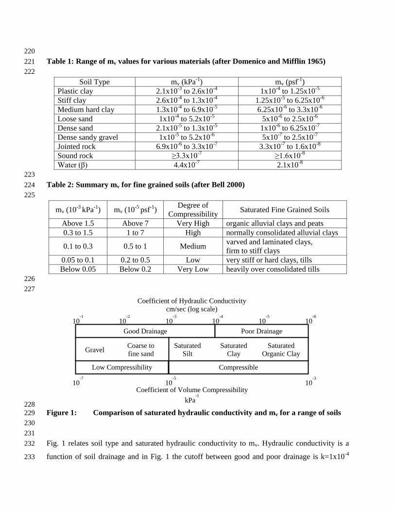
Figure 1: Comparison of saturated hydraulic conductivity and mv for a range of soils 229
230
231
Fig. 1 relates soil type and saturated hydraulic conductivity to mv. Hydraulic conductivity is a 232
function of soil drainage and in Fig. 1 the cutoff between good and poor drainage is k=1x10⁻⁴
233
10-2
10-3
10-4
10-6
10-5
Good Drainage Poor Drainage
Low Compressibility Compressible
10-1
Coefficient of Hydraulic Conductivity cm/sec (log scale)
Gravel
10-7
10-5
10-3
Coefficient of Volume Compressibility
kPa-1
Coarse to
fine sand Saturated
Silt Saturated
Clay Saturated
Organic Clay
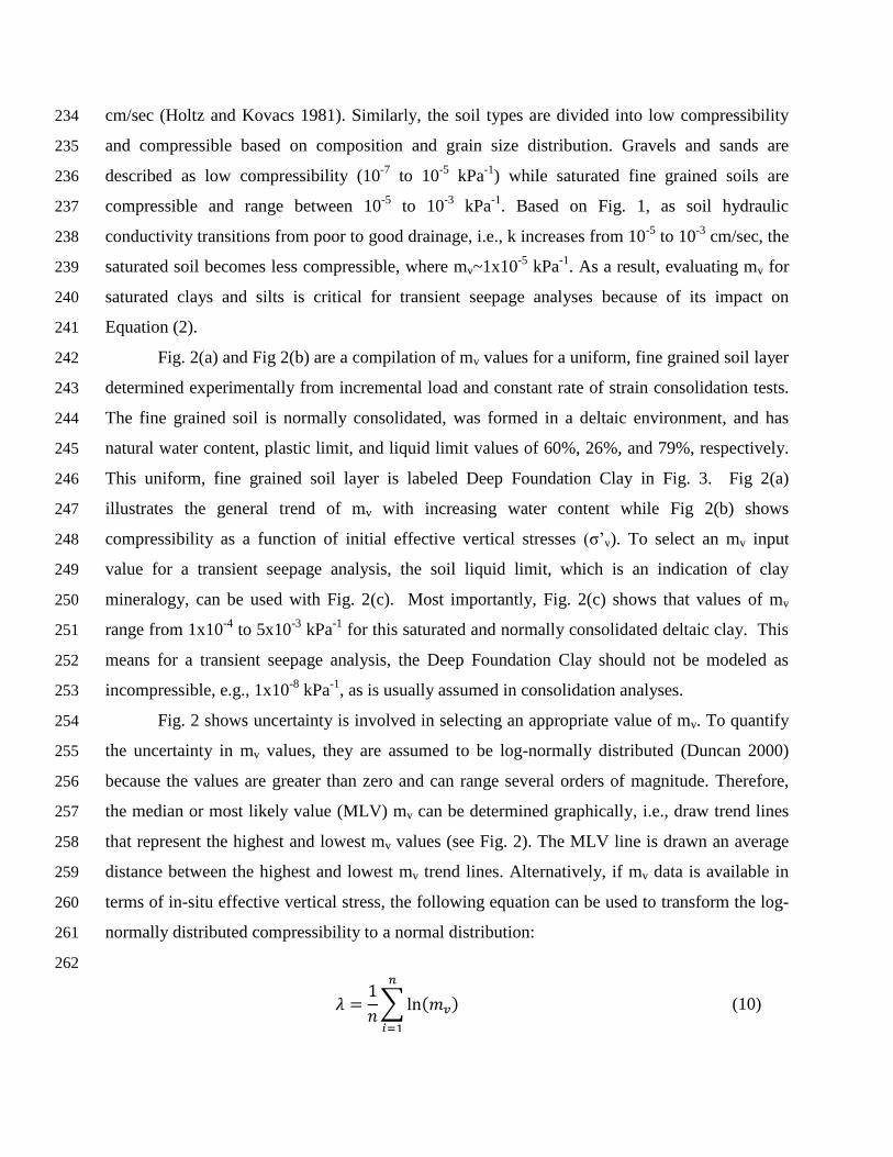
cm/sec (Holtz and Kovacs 1981). Similarly, the soil types are divided into low compressibility 234
and compressible based on composition and grain size distribution. Gravels and sands are 235
described as low compressibility (10-7
to 10-5
kPa-1
) while saturated fine grained soils are 236
compressible and range between 10-5
to 10-3
kPa-1
. Based on Fig. 1, as soil hydraulic 237
conductivity transitions from poor to good drainage, i.e., k increases from 10-5
to 10-3
cm/sec, the 238
saturated soil becomes less compressible, where mv~1x10⁻⁵
kPa-1
. As a result, evaluating mv for 239
saturated clays and silts is critical for transient seepage analyses because of its impact on 240
Equation (2). 241
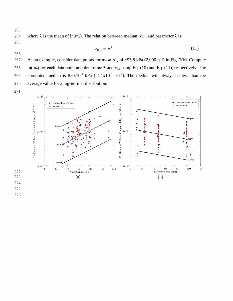
Fig. 2(a) and Fig 2(b) are a compilation of mv values for a uniform, fine grained soil layer 242
determined experimentally from incremental load and constant rate of strain consolidation tests. 243
The fine grained soil is normally consolidated, was formed in a deltaic environment, and has 244
natural water content, plastic limit, and liquid limit values of 60%, 26%, and 79%, respectively. 245
This uniform, fine grained soil layer is labeled Deep Foundation Clay in Fig. 3. Fig 2(a) 246
illustrates the general trend of mv with increasing water content while Fig 2(b) shows 247
compressibility as a function of initial effective vertical stresses (σ’v). To select an mv input 248
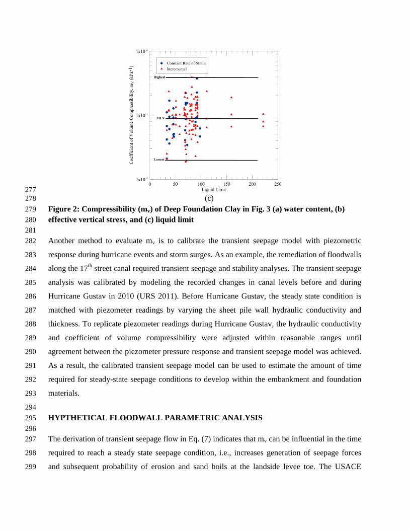
value for a transient seepage analysis, the soil liquid limit, which is an indication of clay 249
mineralogy, can be used with Fig. 2(c). Most importantly, Fig. 2(c) shows that values of mv 250
range from 1x10⁻⁴
to 5x10⁻³
kPa-1
for this saturated and normally consolidated deltaic clay. This 251
means for a transient seepage analysis, the Deep Foundation Clay should not be modeled as 252
incompressible, e.g., 1x10⁻⁸
kPa-1
, as is usually assumed in consolidation analyses. 253
Fig. 2 shows uncertainty is involved in selecting an appropriate value of mv. To quantify 254
the uncertainty in mv values, they are assumed to be log-normally distributed (Duncan 2000) 255
because the values are greater than zero and can range several orders of magnitude. Therefore, 256
the median or most likely value (MLV) mv can be determined graphically, i.e., draw trend lines 257
that represent the highest and lowest mv values (see Fig. 2). The MLV line is drawn an average 258
distance between the highest and lowest mv trend lines. Alternatively, if mv data is available in 259
terms of in-situ effective vertical stress, the following equation can be used to transform the log-260
normally distributed compressibility to a normal distribution: 261
262
∑ ( )
(10)
263
where λ is the mean of ln(mv). The relation between median, x0.5, and parameter λ is: 264
265
(11)
266
As an example, consider data points for mv at σ’v of ~95.8 kPa (2,000 psf) in Fig. 2(b). Compute 267
ln(mv) for each data point and determine λ and x0.5 using Eq. (10) and Eq. (11), respectively. The 268
computed median is 8.6x10⁻⁴
kPa ( 4.1x10⁻⁵
psf-1
). The median will always be less than the 269
average value for a log-normal distribution. 270
271
272
(a) (b) 273
274
275
276
277
(c) 278
Figure 2: Compressibility (mv) of Deep Foundation Clay in Fig. 3 (a) water content, (b) 279
effective vertical stress, and (c) liquid limit 280
281
Another method to evaluate mv is to calibrate the transient seepage model with piezometric 282
response during hurricane events and storm surges. As an example, the remediation of floodwalls 283
along the 17th
street canal required transient seepage and stability analyses. The transient seepage 284
analysis was calibrated by modeling the recorded changes in canal levels before and during 285
Hurricane Gustav in 2010 (URS 2011). Before Hurricane Gustav, the steady state condition is 286
matched with piezometer readings by varying the sheet pile wall hydraulic conductivity and 287
thickness. To replicate piezometer readings during Hurricane Gustav, the hydraulic conductivity 288
and coefficient of volume compressibility were adjusted within reasonable ranges until 289
agreement between the piezometer pressure response and transient seepage model was achieved. 290
As a result, the calibrated transient seepage model can be used to estimate the amount of time 291
required for steady-state seepage conditions to develop within the embankment and foundation 292
materials. 293
294
HYPTHETICAL FLOODWALL PARAMETRIC ANALYSIS 295
296
The derivation of transient seepage flow in Eq. (7) indicates that mv can be influential in the time 297
required to reach a steady state seepage condition, i.e., increases generation of seepage forces 298
and subsequent probability of erosion and sand boils at the landside levee toe. The USACE 299
(2000) defines exit gradients of 0.5 to 0.8 to represent conditions favorable for erosion and sand 300
boils. To develop high exit gradients, seepage forces must travel from floodside to landside of 301
the levee to increase pore-water pressures and thus exit gradients. As a result, a hypothetical 302
floodwall system is used to perform parametric analyses of mv, hydraulic conductivity, and levee 303
geometry to illustrate the importance of mv on landside pore-water pressures. 304
The software SEEP\W (Geo-Slope 2007) was used for the two-dimensional (2D) analysis 305
of seepage and hydraulic effects. The CAD-based user interface and automated solver facilitate 306
input of 2D geometries to evaluate field seepage conditions. SEEP/W is a finite element model 307
that can analyze groundwater seepage and excess pore-water pressure dissipation estimated from 308
a stress-deformation analysis within porous materials. SEEP/W can model both saturated and 309
unsaturated flow, which allows it to analyze seepage as a function of time and to consider such 310
processes as infiltration or wetting front migration. 311
Fig. 3 shows a hypothetical floodwall system consisting of a reinforced concrete 312
floodwall and a supporting sheet pile extending to a depth of -4 m (NAVD88). The sheetpile cuts 313
off seepage or impedes seepage in the upper clay layer so the focus of the seepage analysis is 314
flow through the lower clay layer (see Fig. 3). A deep excavation or burrow pit is modeled 15 m 315
floodside from the floodwall and a clay plug, e.g., clay filled excavation, is modeled 30 m 316
landside of the floodwall. Because the excavation fill is clean sand and hydraulically connected 317
to the lower clay layer, underseepage can occur below the floodwall. The hypothetical 318
excavation represents a possible floodside borrow pit or old river channel which is hydraulically 319
connected to the substratum underlying the levee and clay blanket for this parametric study. The 320
hypothetical excavation is filled with clean sand because preliminary analyses show that 321
excavation filled soils, e.g., k=10-5
cm/sec, did not cause landside pore-water pressures to 322
increase, which indicates that seepage flow from the floodside must occur to develop landside 323
uplift pressures. 324
325
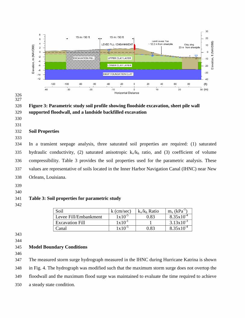
326 327
Figure 3: Parametric study soil profile showing floodside excavation, sheet pile wall 328
supported floodwall, and a landside backfilled excavation 329
330
331
Soil Properties 332
333
In a transient seepage analysis, three saturated soil properties are required: (1) saturated 334
hydraulic conductivity, (2) saturated anisotropic kv/kh ratio, and (3) coefficient of volume 335
compressibility. Table 3 provides the soil properties used for the parametric analysis. These 336
values are representative of soils located in the Inner Harbor Navigation Canal (IHNC) near New 337
Orleans, Louisiana. 338
339
340
Table 3: Soil properties for parametric study 341
342
Soil k (cm/sec) kv/kh Ratio mv (kPa-1
)
Levee Fill/Embankment 1x10⁻⁵
0.83 8.35x10⁻⁴
Excavation Fill 1x10⁻¹
1 3.13x10⁻³
Canal 1x10⁻⁵
0.83 8.35x10⁻⁴
343
344
Model Boundary Conditions 345
346
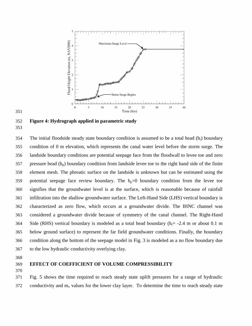
The measured storm surge hydrograph measured in the IHNC during Hurricane Katrina is shown 347
in Fig. 4. The hydrograph was modified such that the maximum storm surge does not overtop the 348
floodwall and the maximum flood surge was maintained to evaluate the time required to achieve 349
a steady state condition. 350
351
Figure 4: Hydrograph applied in parametric study 352
353
The initial floodside steady state boundary condition is assumed to be a total head (ht) boundary 354
condition of 0 m elevation, which represents the canal water level before the storm surge. The 355
landside boundary conditions are potential seepage face from the floodwall to levee toe and zero 356
pressure head (hp) boundary condition from landside levee toe to the right hand side of the finite 357
element mesh. The phreatic surface on the landside is unknown but can be estimated using the 358
potential seepage face review boundary. The hp=0 boundary condition from the levee toe 359
signifies that the groundwater level is at the surface, which is reasonable because of rainfall 360
infiltration into the shallow groundwater surface. The Left-Hand Side (LHS) vertical boundary is 361
characterized as zero flow, which occurs at a groundwater divide. The IHNC channel was 362
considered a groundwater divide because of symmetry of the canal channel. The Right-Hand 363
Side (RHS) vertical boundary is modeled as a total head boundary (ht= -2.4 m or about 0.1 m 364
below ground surface) to represent the far field groundwater conditions. Finally, the boundary 365
condition along the bottom of the seepage model in Fig. 3 is modeled as a no flow boundary due 366
to the low hydraulic conductivity overlying clay. 367
368
EFFECT OF COEFFICIENT OF VOLUME COMPRESSIBILITY 369
370
Fig. 5 shows the time required to reach steady state uplift pressures for a range of hydraulic 371
conductivity and mv values for the lower clay layer. To determine the time to reach steady state 372
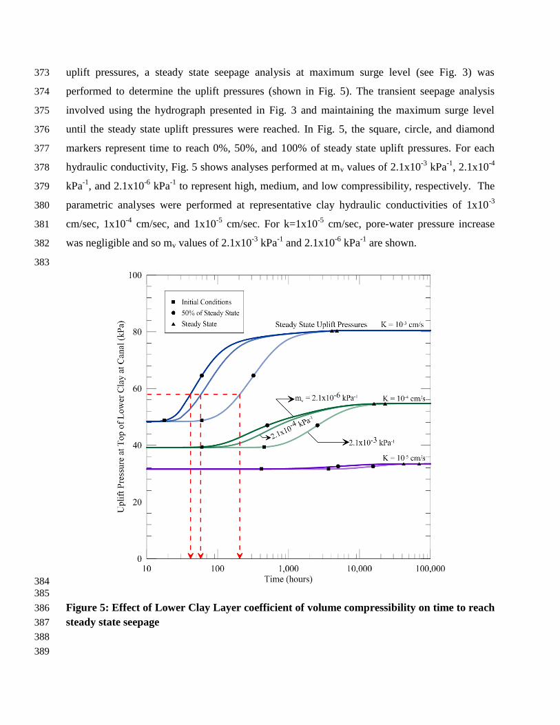
uplift pressures, a steady state seepage analysis at maximum surge level (see Fig. 3) was 373
performed to determine the uplift pressures (shown in Fig. 5). The transient seepage analysis 374
involved using the hydrograph presented in Fig. 3 and maintaining the maximum surge level 375
until the steady state uplift pressures were reached. In Fig. 5, the square, circle, and diamond 376
markers represent time to reach 0%, 50%, and 100% of steady state uplift pressures. For each 377
hydraulic conductivity, Fig. 5 shows analyses performed at mv values of 2.1x10⁻³
kPa-1
, 2.1x10⁻⁴
378
kPa-1
, and 2.1x10⁻⁶
kPa-1
to represent high, medium, and low compressibility, respectively. The 379
parametric analyses were performed at representative clay hydraulic conductivities of 1x10⁻³
380
cm/sec, 1x10⁻⁴
cm/sec, and 1x10⁻⁵
cm/sec. For k=1x10⁻⁵
cm/sec, pore-water pressure increase 381
was negligible and so mv values of 2.1x10⁻³
kPa-1
and 2.1x10⁻⁶
kPa-1
are shown. 382
383
384
385
Figure 5: Effect of Lower Clay Layer coefficient of volume compressibility on time to reach 386
steady state seepage 387
388
389
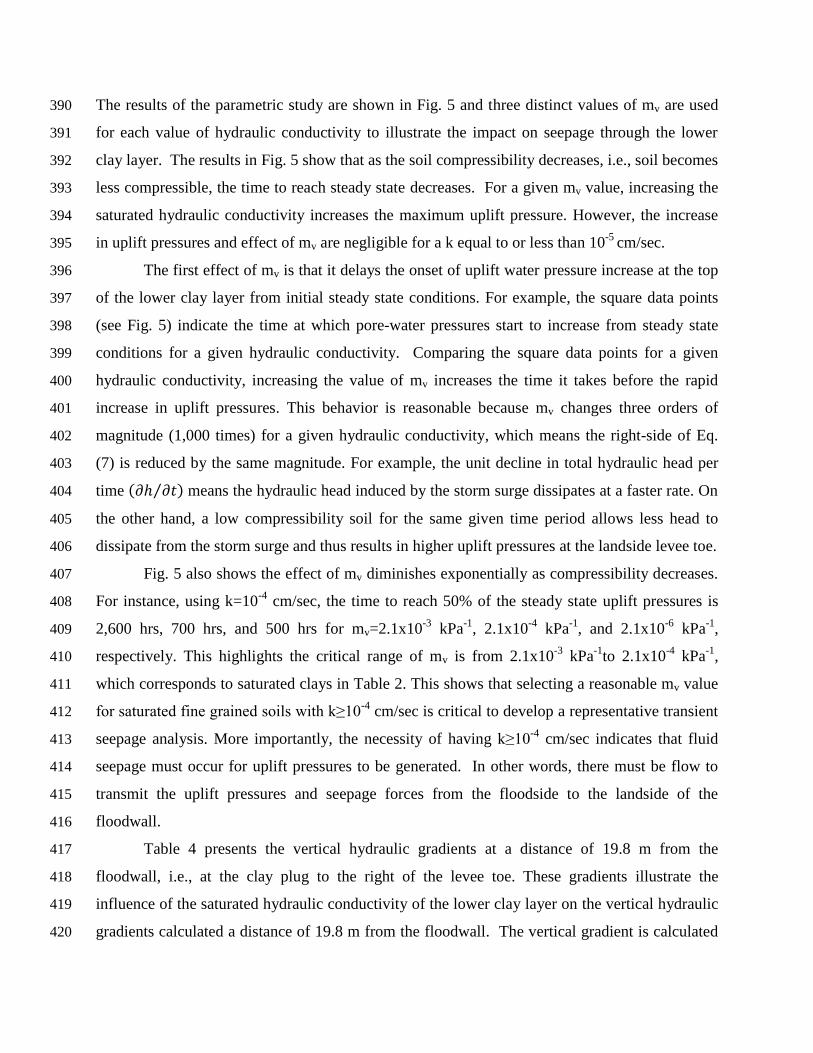
The results of the parametric study are shown in Fig. 5 and three distinct values of mv are used 390
for each value of hydraulic conductivity to illustrate the impact on seepage through the lower 391
clay layer. The results in Fig. 5 show that as the soil compressibility decreases, i.e., soil becomes 392
less compressible, the time to reach steady state decreases. For a given mv value, increasing the 393
saturated hydraulic conductivity increases the maximum uplift pressure. However, the increase 394
in uplift pressures and effect of mv are negligible for a k equal to or less than 10-5
cm/sec. 395
The first effect of mv is that it delays the onset of uplift water pressure increase at the top 396
of the lower clay layer from initial steady state conditions. For example, the square data points 397
(see Fig. 5) indicate the time at which pore-water pressures start to increase from steady state 398
conditions for a given hydraulic conductivity. Comparing the square data points for a given 399
hydraulic conductivity, increasing the value of mv increases the time it takes before the rapid 400
increase in uplift pressures. This behavior is reasonable because mv changes three orders of 401
magnitude (1,000 times) for a given hydraulic conductivity, which means the right-side of Eq. 402
(7) is reduced by the same magnitude. For example, the unit decline in total hydraulic head per 403
time ( ⁄ ) means the hydraulic head induced by the storm surge dissipates at a faster rate. On 404
the other hand, a low compressibility soil for the same given time period allows less head to 405
dissipate from the storm surge and thus results in higher uplift pressures at the landside levee toe. 406
Fig. 5 also shows the effect of mv diminishes exponentially as compressibility decreases. 407
For instance, using k=10-4
cm/sec, the time to reach 50% of the steady state uplift pressures is 408
2,600 hrs, 700 hrs, and 500 hrs for mv=2.1x10⁻³
kPa-1
, 2.1x10⁻⁴
kPa-1
, and 2.1x10⁻⁶
kPa-1
, 409
respectively. This highlights the critical range of mv is from 2.1x10⁻³
kPa-1
to 2.1x10⁻⁴
kPa-1
, 410
which corresponds to saturated clays in Table 2. This shows that selecting a reasonable mv value 411
for saturated fine grained soils with k≥10-4
cm/sec is critical to develop a representative transient 412
seepage analysis. More importantly, the necessity of having k≥10-4
cm/sec indicates that fluid 413
seepage must occur for uplift pressures to be generated. In other words, there must be flow to 414
transmit the uplift pressures and seepage forces from the floodside to the landside of the 415
floodwall. 416
Table 4 presents the vertical hydraulic gradients at a distance of 19.8 m from the 417
floodwall, i.e., at the clay plug to the right of the levee toe. These gradients illustrate the 418
influence of the saturated hydraulic conductivity of the lower clay layer on the vertical hydraulic 419
gradients calculated a distance of 19.8 m from the floodwall. The vertical gradient is calculated 420
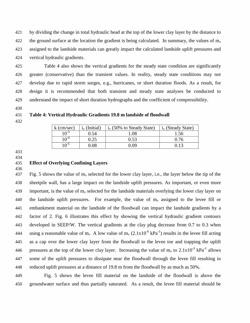
by dividing the change in total hydraulic head at the top of the lower clay layer by the distance to 421
the ground surface at the location the gradient is being calculated. In summary, the values of mv 422
assigned to the landside materials can greatly impact the calculated landside uplift pressures and 423
vertical hydraulic gradients. 424
Table 4 also shows the vertical gradients for the steady state condition are significantly 425
greater (conservative) than the transient values. In reality, steady state conditions may not 426
develop due to rapid storm surges, e.g., hurricanes, or short duration floods. As a result, for 427
design it is recommended that both transient and steady state analyses be conducted to 428
understand the impact of short duration hydrographs and the coefficient of compressibility. 429
430
Table 4: Vertical Hydraulic Gradients 19.8 m landside of floodwall 431
432
k (cm/sec) iv (Initial) iv (50% to Steady State) iv (Steady State)
10-3
0.54 1.08 1.56
10-4
0.25 0.53 0.76
10-5
0.08 0.09 0.13
433
434
Effect of Overlying Confining Layers 435
436
Fig. 5 shows the value of mv selected for the lower clay layer, i.e., the layer below the tip of the 437
sheetpile wall, has a large impact on the landside uplift pressures. As important, or even more 438
important, is the value of mv selected for the landside materials overlying the lower clay layer on 439
the landside uplift pressures. For example, the value of mv assigned to the levee fill or 440
embankment material on the landside of the floodwall can impact the landside gradients by a 441
factor of 2. Fig. 6 illustrates this effect by showing the vertical hydraulic gradient contours 442
developed in SEEP/W. The vertical gradients at the clay plug decrease from 0.7 to 0.3 when 443
using a reasonable value of mv A low value of mv (2.1x10⁻⁶
kPa-1
) results in the levee fill acting 444
as a cap over the lower clay layer from the floodwall to the levee toe and trapping the uplift 445
pressures at the top of the lower clay layer. Increasing the value of mv to 2.1x10⁻³
kPa-1
allows 446
some of the uplift pressures to dissipate near the floodwall through the levee fill resulting in 447
reduced uplift pressures at a distance of 19.8 m from the floodwall by as much as 50%. 448
Fig. 5 shows the levee fill material on the landside of the floodwall is above the 449
groundwater surface and thus partially saturated. As a result, the levee fill material should be 450

assigned a compressible value, e.g., to 2.1x10⁻³
kPa-1
, of compressibility because the air voids of 451
a partially saturated soil are compressible which is also in agreement with the material 452
compressing when a car was driven on it. When a saturated clay is loaded, it is assumed in 453
geotechnical engineering that water is incompressible so the entire applied load is carried by the 454
pore-water pressures. This assumption is clearly not valid for a partially saturated soil so a 455
compressible value of mv, e.g., 2.1x10⁻³
kPa-1
, should be assigned. 456
457
458 (a) (b) 459
460
Figure 6: Effect of landside levee coefficient of compressibility on vertical hydraulic 461
gradient (a) mv=2.1x10⁻⁸
kPa-1
and (b) mv=8.4x10⁻⁴
kPa-1
462
463
Fig. 7 shows an excavation in the levee fill on the landside of the floodwall near the north 464
end of the IHNC to investigate the soil adjacent to the box culvert in the foreground. The 465
photographs in Fig. 7 show the levee fill in the upper 1.5 to 2 m is lighter color than near the 466
bottom of the excavation indicating a partially saturated condition. Therefore, the levee fill 467
material on the floodside of a floodwall is likely to be partially saturated and should be assigned 468
a compressible value, e.g., to 2.1x10⁻³
kPa-1
, of mv because of the presence of compressible air 469
voids. 470
471
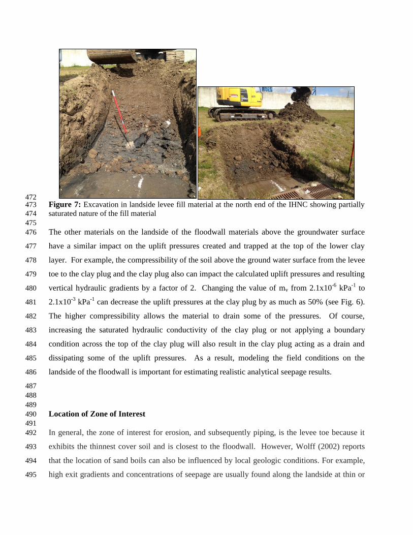
472 Figure 7: Excavation in landside levee fill material at the north end of the IHNC showing partially 473
saturated nature of the fill material 474
475
The other materials on the landside of the floodwall materials above the groundwater surface 476
have a similar impact on the uplift pressures created and trapped at the top of the lower clay 477
layer. For example, the compressibility of the soil above the ground water surface from the levee 478
toe to the clay plug and the clay plug also can impact the calculated uplift pressures and resulting 479
vertical hydraulic gradients by a factor of 2. Changing the value of mv from 2.1x10⁻⁶
kPa-1
to 480
2.1x10⁻³
kPa-1
can decrease the uplift pressures at the clay plug by as much as 50% (see Fig. 6). 481
The higher compressibility allows the material to drain some of the pressures. Of course, 482
increasing the saturated hydraulic conductivity of the clay plug or not applying a boundary 483
condition across the top of the clay plug will also result in the clay plug acting as a drain and 484
dissipating some of the uplift pressures. As a result, modeling the field conditions on the 485
landside of the floodwall is important for estimating realistic analytical seepage results. 486
487
488
489
Location of Zone of Interest 490
491
In general, the zone of interest for erosion, and subsequently piping, is the levee toe because it 492
exhibits the thinnest cover soil and is closest to the floodwall. However, Wolff (2002) reports 493
that the location of sand boils can also be influenced by local geologic conditions. For example, 494
high exit gradients and concentrations of seepage are usually found along the landside at thin or 495
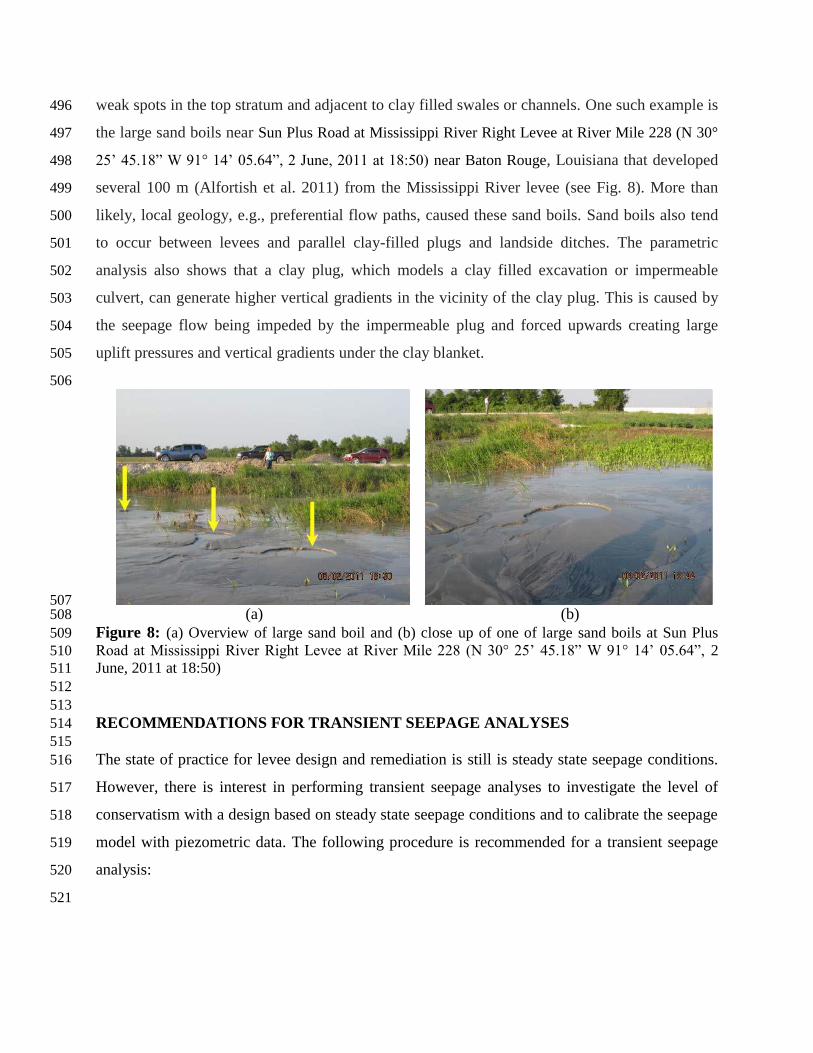
weak spots in the top stratum and adjacent to clay filled swales or channels. One such example is 496
the large sand boils near Sun Plus Road at Mississippi River Right Levee at River Mile 228 (N 30° 497
25’ 45.18” W 91° 14’ 05.64”, 2 June, 2011 at 18:50) near Baton Rouge, Louisiana that developed 498
several 100 m (Alfortish et al. 2011) from the Mississippi River levee (see Fig. 8). More than 499
likely, local geology, e.g., preferential flow paths, caused these sand boils. Sand boils also tend 500
to occur between levees and parallel clay-filled plugs and landside ditches. The parametric 501
analysis also shows that a clay plug, which models a clay filled excavation or impermeable 502
culvert, can generate higher vertical gradients in the vicinity of the clay plug. This is caused by 503
the seepage flow being impeded by the impermeable plug and forced upwards creating large 504
uplift pressures and vertical gradients under the clay blanket. 505
506
507 (a) (b) 508
Figure 8: (a) Overview of large sand boil and (b) close up of one of large sand boils at Sun Plus 509
Road at Mississippi River Right Levee at River Mile 228 (N 30° 25’ 45.18” W 91° 14’ 05.64”, 2 510
June, 2011 at 18:50) 511
512
513
RECOMMENDATIONS FOR TRANSIENT SEEPAGE ANALYSES 514
515
The state of practice for levee design and remediation is still is steady state seepage conditions. 516
However, there is interest in performing transient seepage analyses to investigate the level of 517
conservatism with a design based on steady state seepage conditions and to calibrate the seepage 518
model with piezometric data. The following procedure is recommended for a transient seepage 519
analysis: 520
521
1. Initial steady state conditions: Before performing a transient analysis, the initial pore-522
water pressure regime near the levee must be determined. The floodside and landside 523
groundwater surface before flooding or storm surge should be used to establish the initial 524
phreatic surface through the levee via a steady state analysis. 525
526
2. Transient seepage: The initial steady state pore-water pressure regime is used as a “parent 527
analysis” for the transient analysis and the boundary conditions are no longer constant 528
with time. For example, Fig. 4 shows a storm hydrograph modified from Hurricane 529
Katrina in 2005. The hydrograph is applied as the boundary condition to the floodside 530
surface nodes. Because the flood hydrograph is not known at the time of design, i.e., the 531
hazard event has not occurred, it is recommended to use an agreed upon maximum storm 532
surge level and a reasonable hydrograph. By raising the flood level to maximum and then 533
maintaining the maximum storm surge until steady state conditions develop (see Fig. 4), 534
a parametric study similar to the one in Fig. 5 can be developed. This analysis is 535
performed using the median or most likely value (MLV) of mv using site specific data or 536
values from Tables 1 and 2. Additional analyses using highest conceivable and lowest 537
conceivable mv values can also be performed to develop low and high bounds, 538
respectively, of the time required to reach steady state and magnitude of uplift pressures. 539
In addition, the location or zone of interest for the calculated uplift pressures and vertical 540
gradients can be determined and compared with initial estimates, e.g., levee toe, to ensure 541
reasonable design measures. 542
543
3. Underseepage and exit gradients: An exit hydraulic gradient of 0.85 measured in the 544
vertical direction on the landside of a levee is commonly considered sufficient to initiate 545
sand boil formation. Other field measurements show that sand boils may occur with exit 546
hydraulic gradients in the range of 0.54–1.02 (Daniel 1985). Therefore, using a vertical 547
hydraulic gradient of 0.85, the uplift pressures required to induce heave and sand boils 548
can be back-calculated. Using a graph similar to the shown in Fig. 5 and developed in 549
Step 2, the calculated uplift pressure for a given hydraulic conductivity and mv can be 550
used to estimate the time at which sand boils may develop assuming maximum flood 551
level is approximated. For k=1x10⁻³
cm/sec in Fig. 5, the uplift pressure that induces 552
heave and sand is 58 kPa and the time at which sand boils may develop are 42 hrs, 58 hrs, 553
and 205 hrs for mv=2.1x10⁻³
kPa-1
, 2.1x10⁻⁴
kPa-1
, and 2.1x10⁻⁶
kPa-1
, respectively. This 554
permits levee owners and communities to monitor the levee for seepage distress and plan 555
remedial measures. 556
557
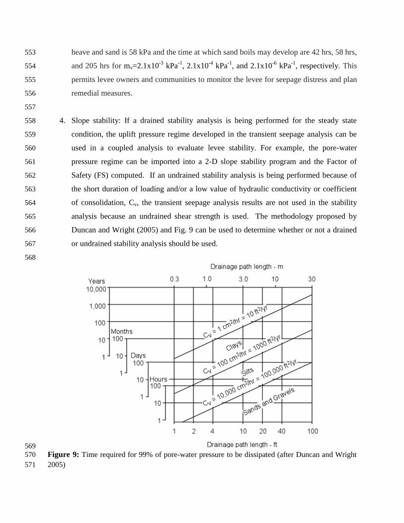
4. Slope stability: If a drained stability analysis is being performed for the steady state 558
condition, the uplift pressure regime developed in the transient seepage analysis can be 559
used in a coupled analysis to evaluate levee stability. For example, the pore-water 560
pressure regime can be imported into a 2-D slope stability program and the Factor of 561
Safety (FS) computed. If an undrained stability analysis is being performed because of 562
the short duration of loading and/or a low value of hydraulic conductivity or coefficient 563
of consolidation, Cv, the transient seepage analysis results are not used in the stability 564
analysis because an undrained shear strength is used. The methodology proposed by 565
Duncan and Wright (2005) and Fig. 9 can be used to determine whether or not a drained 566
or undrained stability analysis should be used. 567
568
569
Figure 9: Time required for 99% of pore-water pressure to be dissipated (after Duncan and Wright 570
2005) 571
572
In summary, steady state and transient seepage each reflect certain soil, e.g., high hydraulic 573
conductivity and compressibility, and boundary conditions, e.g., short duration flood or storm 574
surge. The engineer must determine the appropriate soil conditions and boundary conditions and 575
then determine which method of analysis, e.g., transient or steady state, best simulates field 576
conditions to estimate realistic uplift pressures and hydraulic gradients. 577
578
CONCLUSIONS 579
580
This paper reviews the importance of the coefficient of compressibility on transient seepage 581
analyses using a parametric analysis. The paper also provides guidance on selecting the value of 582
mv and performing transient seepage analyses. The following conclusions were derived from this 583
analysis: 584
585
1. The derivation of transient seepage flow indicates that reducing the value of mv, i.e., 586
making the system incompressible, implicitly transforms the transient seepage 587
analysis to steady state. Also, most seepage analyses assume water is incompressible. 588
The value of mv should not be assumed to be incompressible because mv is a function 589
of both soil skeleton and water compressibility. Even if water is assumed to be 590
incompressible, the soil skeleton usually has a high compressibility especially if it is 591
partially saturated. Therefore, a transient seepage analysis should not be converted to 592
steady state analysis with an erroneously low value of mv. 593
2. General guideline for estimating the coefficient of volume compressibility include 594
laboratory consolidation tests, empirical correlations, soil type, field calibration using 595
piezometers, and field pump tests. In addition, mv is shown to vary, e.g., by an order 596
of magnitude, for the same soil type. To account for uncertainty in the most likey mv 597
value, the highest and lowest values should be used in the analyses. The selected 598
value of mv should also be representative of the in-situ effective vertical stress. 599
3. The parametric analyses show that mv affects the time at which landside uplift 600
pressures start to increase and the magnitude of the uplift pressures. In particular, the 601
effect of mv diminishes as the soil becomes more compressible. As expected, fluid 602
flow must be present for uplift pressures to be generated on the landside of the levee 603
or floodwall. 604
4. Current state of practice for levee underseepage does not require transient seepage 605
analyses, thus making designs potentially conservative and costly. A design 606
procedure for performing transient seepage analyses is provided that incorporates 607
how to estimate material properties, develop initial steady state conditions before 608
applying the flood hydrograph, and using the results to predict an approximate time at 609
which underseepage distress may begin and the zone of interest. 610
611
612
613
ACKNOWLEDGMENTS 614
This material is based upon work supported by the National Science Foundation through a Graduate 615
Research Fellowship to Navid H. Jafari. Any opinions, findings, and conclusions or recommendations 616
expressed in this material are those of the authors and do not necessarily reflect the views of the NSF. 617
618
REFERENCES 619
620
Alfortish, M., Brandon, T. L., Gilbert, R. B., Stark, T. D., and Westerink, J. (2011). 621
"Geotechnical Reconnaissance of the 2011 Flood on the Lower Mississippi River," Geo- 622
engineering Extreme Event Response (GEER) Report, National Science Foundation, 40. 623
Bell, F. G. (2000). Engineering Properties of Soils and Rocks. 4th ed., Blackwell Science, UK. 624
Bennett, P. T.(1946). “The effect of blankets on seepage through pervious foundations.” Trans. 625
Am. Soc. Civ. Eng. 11, Paper No. 2270, 215–252. 626
Cedergren, H. R. (1989). Seepage, Drainage, and Flow Nets, John Wiley and Sons, 627
NY, p 489. 628
Daniel, D. E. (1985). Review of piezometric data for various ranges in the rock island district, 629
USACE Waterways Experiment Station, Vicksburg, Miss. 630
Domenico, P. A., and Mifflin, M. D. (1965). “Water From Low-Permeability Sediments and 631
Land Subsidence.” Water Resources Research, American Geophysical Union, vol. 1, no. 4, 632
563-576. 633
Duncan, J.M. 2000. Factors of safety and reliability in geotechnical engineering. ASCE J. of 634
Geotechnical and Geoenvironmental Engineering, 126(4): 307-316. 635
Duncan, J.M. and Wright, S.G. (2005). Soil strength and slope stability. John Wiley & Sons, 297 636
Freeze, R. A., and Cherry, J. A.(1979). Groundwater, Prentice-Hall Inc., Englewood Cliffs, N.J. 637
Geo-Slope (2007). Seep/W software Users Guide. Geoslope International Ltd., Calgary, 638
Canada. 639
Holtz, R. D. and Kovacs, W. D. (1981). An Introduction to Geotechnical Engineering, Prentice-640
Hall Inc., Englewood Cliffs, N.J. 641
Kruseman, G. P., and Ridder, N. A. (1990). Analysis and Evaluation of Pumping Test Data. 2nd 642
ed., International Institute for Land Reclamation and Improvement (ILRI), Wageningen, 377. 643
Lambe, T. W. and Whitman, R. V. (1969). Soil Mechanics. John Wiley & Sons. 644
Peter, P. (1982). Canal and river levees, Developments of Civil Engineering Vol. 29, 645
Elsevier/North-Holland, Inc., New York. 646
URS JEG JV (2011). "Remediation of Floodwalls on the 17th Street Canal." OFC-05. Dept. of 647
the Army, Washington, D.C. 648
U.S. Army Corps of Engineers (USACE). (2000). “Engineering and design—design and 649
construction of levees.” EM 1110-2-1913, Dept. of the Army, Washington, D.C. 650
U.S. Army Corps of Engineers (USACE). (2005). “Design guidance for levee underseepage.” 651
ETL 1110-2-569, Dept. of the Army, Washington, D.C. 652
Wolff, T. F. (1986). "Design and Performance of Underseepage Controls: A Critical Review." 653
Report ERDC/GSL TR-02-19, U.S. Army Corps of Engineers, Engineer Research and 654
Development Center, (2002), Vicksburg, MS. 655
656
657
658
659
660
661
662
663
664
FIGURE CAPTIONS: 665
666
Figure 1: Comparison of saturated hydraulic conductivity and mv for a range of soils 667
Figure 2: Compressibility (mv) of deltaic clay near New Orleans (a) water content, (b) effective 668
vertical stress, and (c) liquid limit 669
Figure 3: Parametric study soil profile showing floodside excavation, sheet pile wall supported 670
floodwall, and a landside backfilled excavation 671
Figure 4: Hydrograph applied in parametric study 672
Figure 5: Effect of coefficient of compressibility on time to reach steady state seepage 673
Figure 6: Effect of landside levee coefficient of compressibility on vertical hydraulic gradient (a) 674
mv=2.1x10⁻⁸
kPa-1
and (b) mv=8.4x10⁻⁴
kPa-1
675
Figure 7: Excavation in landside levee fill material at the north end of the IHNC showing partially 676
saturated nature of the fill material 677
Figure 8: (a) Overview of large sand boil and (b) close up of one of large sand boils at Sun Plus 678
Road at Mississippi River Right Levee at River Mile 228 (N 30° 25’ 45.18” W 91° 14’ 05.64”, 2 679
June, 2011 at 18:50) 680
Figure 9: Time required for 99% of pore-water pressure to be dissipated (after Duncan and Wright 681
2005) 682
683
684
TABLE CAPTIONS: 685
686
Table 1: Range of mv values (after Domenico and Mifflin 1965) 687
Table 2: Summary mv for clays (after Bell 2000) 688
Table 3: Soil properties for parametric study 689
Table 4: Vertical Hydraulic Gradients 19.8 m landside of floodwall 690
691
692
693
694
695
696
697
698
699