Ye Chen

Effect of Packetized Data on Gain Dynamics in Erbium-

doped Fiber Amplifiers Fed by Live Local Area Network

Traffic

Mémoire

présenté

à la faculté des études supérieures

de l’Université Laval

pour l’obtention

du grade de maître ès sciences (M. Sc.)

Département de génie électrique et de génie informatique

FACULTÉ DE SCIENCES ET DE GÉNIE

UNIVERSITÉ LAVAL

QUÉBEC

Mars 2000

© Ye Chen, 2000

2

Table of Contents

RESUMÉ… … … … … … … … … … … … … … … … … … … … … … … … … … … … .… … … … .4 ABSTRACT… … … … … … … … … … … … … … … … … … … … … … … … … … … .… … … … .5 ACKNOWLEDGMENTS… … … … … … … … … … … … … … … … … … … … … ..… … … … ..6 LIST OF FIGURES… … … … … … … … … … … … … … … … ...… … … … … … … ..… … … … 7 INTRODUCTION… … … … … … … … … … … … … … … … … … … … … … … … … … … … … … … … ..9 CHAPTER 1. NETWORKING AND SELFSIMILARITY… … … … … … … … … … … … … … … … 11 1. Packet Switched Network… … … … … … … … … … … … … … … … … … … … … … ...11 2. Layered Networking Model----OSI Model… … … … … … … … … … … … … … … … .11 3. TCP/IP and Internet… … … … … … … … … … … … … … … … … … … … … … … … … 12 4. Ethernet… … … … … … … … … … … … … … … … … … … … … … … … … … … … … ..14 5. Optical Networking… … … … … … … … … … … … … … … … … … … … … … … … … 19 6. IP over WDM or DWDM… … … … … … … … … … … … … … … … … … … … … … ..28 7. Self-similar Nature of the Network Traffic… … … … … … … … … … … … … … … ..30 CHAPTER 2. ERBIUM-DOPED FIBER AMPLIFIER… … … … … … … … … … … … .… .33 Introduction… … … … … … … … … … … … … … … … … … … … … … … … … … … … … .33 1. Basic EDFA Configuration… … … … … … … … … … … … … … … … … … … … … ...35 2. Saleh and Sun’s Model… … … … … … … … … … … … … … … … … … … … … … … ..37 3. Bononi and Rusch’s Reservoir Model… … … … … … … … … … … … … … … … … ..39 4. Approximate Solutions… … … … … … … … … … … … … … … … … … … … … … .… .41 5. EDFA Cascade… … … … … … … … … … … … … … … … … … … … … … … … … … ..47 6. Gain-Clamped EDFA… … … … … … … … … … … … … … … … … … … … … … … … 48 7. Cross-Gain Modulation… … … … … … … … … … … … … … … … … … … … … … … .51 CHAPTER 3. EXPERIMENTAL SETUP… … … … … … … … … … … … … … ...… … … … .53 1. General Setup… … … … … … … … … … … … … … … … … … … … … … … … … … ...53 2. Ethernet Optical Transmitter… … … … … … … … … … … … … … … … … … … … … 54 3. 3 dB Coupler… … … … … … … … … … … … … … … … … … … … … … … … … … … 59 4. EDFA… … … … … … … … … ...… … … … … … … … … … … … … … … … … … … … 60 5. Circulator and Bragg Grating… … … … … … … … … … … … … … … … … … … … ..60 6. Photodetector… … … … … … … ...… … … … … … … … … … … … … … … … … … … 61 7. Data Acquisition Hardware and Software… … … … … … … … … … … … … … … ...64 CHAPTER 4. EXPERIMENTAL RESULTS… … … … … … … … … … … … .… … … … … … … … ..68 Introduction… … … … … … … … … … … … … … … … … … … … … … … … … … … … … .68 1. Time Response to Variable Data … … … … … … … … … … … … … … … … … … … ..69 2. Ethernet Data … … … … … … … … … … … … ..… … … … … … … … … … … … … … ..71 3. Measurements of Gain Swings Comparison with Bononi’s Artificial Traffic… … ..73 4. Gain Clamping… … … … … … … … … … … … … … … … … … … … … … … … … … ...75 5. Comparison with Results for Artificial Ethernet Data… … … … … … … … … … … ..79 6. Experimental Implementation… … … … … … … … … … … … … … … … … … … … ...80 CHAPTER 5. CONCLUSIONS… … … … … … … … … … … … … … … … … … … … … … ..81

3

1. What was achieved… … … … … … … … … … … … … … … … … … … … … … … … ..81 2. Possible follow-up work… … … … … … … … … … … … … … … … … … … … … … ..82 REFERENCES… … … … … … … … … … … … … … … … … … … … … … … … … .… … .… ...83 APPENDIX I. The Ethernet Optical— Electrical Transmitter Circuit Scheme… … … .87 APPENDIX II. AUI on 10 Base-T Ethernet Hub… … … … … … … … … … … … … … … .89

4

RESUMÉ

La réponse des amplificateurs de fiber dopés à l’erbium (EDFAs) aux changements non-

périodiques des canaux d'entrée (dus au canal “add/drop”, à la reconfiguration de réseau, aux

coupes de fiber, ou le traffic en paquet) a été l'étude de beaucoup de recherche récente [1].

L'excursion du gain dans un amplificateur du aux changements dans les canaux d'entrée mène

possiblement à de larges oscillations du rapport signal/bruit optique de sortie (OSNR). Étant

donné la popularité extrême d'Internet, nous prévoyons que les futurs réseaux optiques devront

supporter les données Internet “de mode indigène”, c’est-à-dire des données qui sont transmises

par paquets et qui n’ont pas la modulation continue caractéristique du multiplexage temporel de

signaux. Pour cette raison, la recherche s'est concentrée sur la réponse des EDFAs à des données

qui se caractérisent par des périodes de modulation et de silence (périodes MARCHE-ARRÊT).

Pour la première fois, nous avons mesuré la réponse d'EDFAs aux données de type Ethernet à 10

Mb/s. De plus, nous avons vérifié des résultats théoriques où des données en paquet étaient

modelisées avec des caractéristiques autosimilaires. Nos mesures montrent une variation

substantielle de gain après cinq amplificateurs en cascade. Nous avons également asservi le gain

(boucle de “feedback”) pour stabiliser la puissance de sortie. La méthode s’est révélée

extrêmement pertinente contre les excursions de gain apparaissant lors de la transmission de

paquets Ethernet.

------------------------------ -------------------------------

Ye Chen Prof. Leslie Ann Rusch

Étudiant à la maîtrise Directrice de recherche

5

ABSTRACT

The response of erbium doped fiber amplifiers (EDFAs) to non-periodic changes in the input

channels (due to channel add/drop, network reconfiguration, fiber cuts, or packetized traffic) has

been the subject of much recent research [1]. Gain excursion in an amplifier due to changes in

the input channels leads to possibly wide swings in the output optical signal-to-noise ratio

(OSNR). Given the extreme popularity of the Internet, we anticipate that future optical networks

will be increasingly required to support “native mode” Internet data, that is, data that is

transmitted in packets do not have the continuous modulation that is characteristic of time

division multiplexing. For this reason, research has focused on the EDFA response to data that is

characterized by periods of modulation and silence (ON and OFF times).

For the first time we have measured the response of EDFAs to live Ethernet data at 10 Mb/s and

verified previous theoretical results where packetized data is modeled as having self-similar

characteristics. Our measurements show substantial output power variation after five amplifiers

in a cascade. We have also implemented gain clamping to combat the output power variation.

Gain clamping is extremely effective against output power variation due to packetized input.

6

Acknowledgements

During my two and half years’ Master study at Laval University, Dr. Leslie Ann Rusch kept on

guiding and encouraging me all the time, she is so kind and patient for my study and research

like a good friend or an elder sister. She helped me conquer lots of trouble when I first came to

Quebec. Though Quebec’s winters are severe, I always feel warm to be her student. To some

degree, I regard this work as my Christmas gift for her before she left for working in USA in

December 1999.

I am also obliged to express my special thanks to Dr. Jean-François Cliche who helped me

tremendously on the Ethernet transmitter and EDFAs’ PCBs. We worked together all day long

for a couple of weeks on circuits before I can start the measurements.

Thanks for Dr. Miroslav Karasek’s theoretical directions and experimental cooperation.

Special thanks for Dr. Bo Wen (Washington State University) who suggested me lots of good

idea on networking.

What’s more, I’d like to thank the group of Centre d'Optique, Photonique et Laser (COPL), for

the best research environment, friendly cooperation and brotherhood here.

7

List of Figures

Figure 1-1. The OSI model includes 7 layers that define network functionality… … … … … … ...12 Figure 1-2. Internet… … … … … … … … … … … … … … … … … … … … … … … … … … … … … … 12 Figure 1-3. TCP/IP and Internet architecture… … … … … … … … … … … … … … … … … … … ...13 Figure 1-4. TCP/IP suite and OSI layers… … … … … … … … … … … … … … … … … … … … .… ..14 Figure 1-5. The jam signal ensures all nodes recognize a collision… … … … … … … … … … … ...15 Figure 1-6 CSMA/CD Flow Chart… … … … … … … … … … … … … … … … … … … … … … ..… ...16 Figure 1-7. High-Speed Ethernet options and switching technologies offer more bandwidth to

users and workgroups… … … … … … … … … … … … … … … … … … … … … … … … .17 Figure 1-8. Gigabit Ethernet protocol stack… … … … … … … … … … … … … … … … … … … … ...18 Figure 1-9. End-to-End Wavelength Services… … … … … … … … … … … … … … … … … … … ...19 Figure 1-10. Wavelength Division Multiplexing… … … … … … … … … … … … … … … … … … ..19 Figure 1-11. Development Milestones… … … … … … … … … … … … … … … … … … … … … … ..21 Figure 1-12. Usage of Erbium-doped Fiber Amplifier (EDFA)… … … … … … … … … … … … ....23 Figure 1-13. DWDM Systems… … … … … … … … … … … … … … … … … … … … … … … … … ...24 Figure 1-14. ITU Channel Spacing… … … … … … … … … … … … … … … … … … … … … … … ....24 Figure 1-15. Unidirectional and Bi-directional DWDM… … … … … … … … … … … … … … … ....25 Figure 1-16. In-Fiber Bragg Grating Technology: Optical A/D Multiplexer… … … … … … … ....26 Figure 1-17. Key Functional Blocks for WDM Transport Systems… … … … … … … … … … … ..27 Figure 1-18. Network Bandwidth Prediction… … … … … … … … … … … … … … … … … … … .… 28 Figure 1-19. IP Transport Alternatives… … … … … … … … … … … … … … … … … … … … … … ..29 Figure 1-20. IP over DWDM… … … … … … … … … … … … … … … … … … … … … … … … … … .30 Figure 1-21. Pictorial Proof of Self-Similarity… … … … … … … … … … … … … … … … … … … . 31 Figure 2-1 (a) amplifiers in point-to-point transmission system (b) amplifiers in networks… … .34 Figure 2-2. Basic EDFA Configuration… … … … … … … … … … … … … … … … … … … … … … .35 Figure 2-3. Erbium Energy Level… … … … … … … … … … … … … … … … … … … … … … … … ..37 Figure 2-4. Reservoir model… … … … … … … … … … … … … … … … … … … … … … … … … … ..40 Figure 2-5. A simple WDM system… … … … … … … … … … … … … … … … … … … … … … … ...43 Figure 2-6. Add/Drop simulation using Reservoir Model … … … … … … … … … … … … … … … 44 Figure 2-7. Our Add/Drop Experiment… … … … … … … … … … … … … … … … … … … … … … ..44 Figure 2-8. Sun’s Results… … … … … … … … … … … … … … … … … … … … … … … … … … … ..45 Figure 2-9. Real case and approximations… … … … … … … … … … … … … … … … … … … … … 46 Figure 2-10. Some Fit Methods… … … … … … … … … … … … … … … … … … … … … … … … … .46 Figure 2-11. Gain-Clamped EDFA… … … … … … … … … … … … … … … … … … … … … … … … 48 Figure 2-12. A simple and practical Gain-clamped EDFA design… … … … … … … … … … … … 48 Figure 2-13. Gain versus average inversion and wavelength… … … … … … … … … … … … … … 49 Figure 2-14. Setup… … … … … … … … … … … … … … … … … … … … … … … … … … … … … .… 51 Figure 2-15. Cross-Gain Modulation… … … … … … … … … … … … … … … … … … … … … … … .51 Figure 3-1. Experiment Setup… … … … … … … … … … … … … … … … … … … … … … … … … ....53 Figure 3-2. Logical Structure of the Ethernet Optical Transmitter… … … … … … … … … … … ...54 Figure 3-3. AD96685BR ECL Comparator… … … … … … … … … … … … … … … … … … … … ..55 Figure 3-4. FMM3171VI Laser Driver… … … … … … … … … … … … … … … … … … … … … … ..56 Figure 3-5. FLD5F8LK DFB Laser… … … … … … … … … … … … … … … … … … … … … … … ...57 Figure 3-6. FLD5F8LK Laser’s Spectrum… … … … … … … … … … … … … … … … … … … ..… ..57 Figure 3-7. Transmission Performance in packet level … … … … … … … … … … … … … … … ....58

8

Figure 3-8. Laser’s Transient response in bit level… … … … … … … … … … … … … … … … … ..58 Figure 3-9. Overview of the Ethernet Transmitter… … … … … … … … … … … … … … … … … … 59 Figure 3-10. 3dB Coupler… … … … … … … … … … … … … … … … … … … … … … … … … … … .59 Figure 3-11. EDFA… … … … … … … … … … … … … … … … … … … … … … … … … … … … … … 60 Figure 3-12. EDFA ASE Character… … … … … … … … … … … … … … … … … … … … … … … .60 Figure 3-13. Optical Circulator and Bragg Grating… … … … … … … … … … … … … … … … … ..61 Figure 3-14. ANTEL ARX-GP amplified ultra high-speed photodetector… … … … … … … … … ..61 Figure 3-15. Data Acquisition Scheme… … … … … … … … … … … … … … … … … … … … … … ..62 Figure 3-16. BNC-2110 Accessory… … … … … … … … … … … … … … … … … … … … … … … ....63 Figure 3-17. Front Panel of BNC-2110… … … … … … … … … … … … … … … … … … … … … … .63 Figure 3-18. NI-DAQ driver for Windows… … … … … … … … … … … … … … … … … … … … ....65 Figure 3-19. Relationship between the Programming Environment, NI-DAQ, and the

Hardware… … … … … … … … … … … … … … … … … … … … … … … … … … … … ....66 Figure 3-20. LabVIEW DAQ Software Interface… … … … … … … … … … … … … … … … … … ..66 Figure 3-21. Read and Convert Program Interface… … … … … … … … … … … … … … … … ...… .67 Figure 4-1. Time evolution of photodetector voltage … … … … … … … … … … … … … … … ...… 69 Figure 4-2. Time response of the EDFAs Cascade.… … … … … … … … .… … … … … … … … … ..70 Figure 4-3. The effectiveness of gain clamping … … … … … … … … … … … … … … … … … ...… .70 Figure 4-4. Traffic Generation … … … … ...… … … … … … … … .… … … … … … … … … … … … ..71 Figure 4-5. PDF of the 1st EDFA .… … … … … … … … ...… … … … … … … … … … … … … … … ..73 Figure 4-6. PDF of the 3rd EDFA … … … … … … … … … … … ...… … … … … … … … … … ..… ..73 Figure 4-7. Output of the 5th EDFA … … … … … … … … … … … … … … … … … … … … … … … .74 Figure 4-8. PDF broadens along the EDFA cascade … … … … … … … … … … … … … … … … … 75 Figure 4-9. Time evolution of EDFA 3 and EDFA 5… … … … ..… … … … … … … … … … … … .76 Figure 4-10. Clamping also reduces the gain swing in the cascade… … … … … … … .… … .… … 77 Figure 4-11. Output of EDFA 1 under clamped and unclamped cases… … … … … … .… … … … 77 Figure 4-12. Probability density function of EDFA 3 and 5… … … … … … … … … … … … … … .78 Figure 4-13. Bononi’s Setup with artificial traffic… … … … … … … … … … … … … … … … … … 79 Figure 4-14. Bononi’s Results… … … … … … … … … … … … … … … … … … … … ..… … … … … .79

9

Introduction

Wavelength division multiplexing (WDM) technology employing erbium-doped fiber amplifiers

(EDFAs) provides a platform for significant improvement in network bandwidth capacity. WDM

will play a dominant role in backbone infrastructure supporting the next generation high-speed

networks. Fast signal power transients caused by cross-gain saturation effects pose a serious

limitation in amplified WDM transmission networks. Whereas most previous analysis on cross-

gain saturation in EDFAs focuses on circuit-switched scenarios, we address links carrying data

packets. When the number of WDM channels transmitted through a circuit-switching network

varies due to network reconfiguration or channel failure, channel addition/removal will tend to

perturb signals at the surviving channels that share all or part of the route. Although this

perturbation will generally be small in a single amplifier, it will grow rapidly along a cascade.

Power transients in the surviving channels can cause severe service impairment due to either

inadequate eye opening or the appearance of optical nonlinearities [1-3]. Several solutions to this

problem have been proposed and experimentally verified. These include fast pump control [4, 5],

fast link control by insertion of a control channel [6], and gain clamping by an all-optical

feedback loop [7, 8].

Recent traffic measurements from working packet networks (including Ethernet local area

networks, wide area networks, integrated services digital network, and variable bit rate video

over asynchronous transfer mode) have shown features of self-similarity: that is, realistic packet

network traffic looks the same when measured over time scales ranging from milliseconds to

seconds to minutes and hours [9-11]. It has been concluded that a superposition of many

ON/OFF sources or packet-trains with strictly alternating ON- and OFF-periods with infinite

variance produces aggregate network traffic that is self-similar. When such packet traffic is

directly transmitted on the WDM channels, as in the case of Internet Protocol (IP), long empty

slot intervals may give enough time to fiber amplifiers to reach gains greatly exceeding the

average values. This can in turn lead to significant variation in output power and optical signal-

to-noise ratio (OSNR). This effect accumulates along a cascade of fiber amplifiers in the same

way as the fast power transients in the circuit-switching scenario. The effect of WDM traffic

10

statistics on the output power and optical OSNR swings in a cascade of five erbium-doped fiber

amplifiers (EDFAs) of standard design has been theoretically investigated in [12, 13]. The results

of the simulations indicate that substantial power and OSNR swings occur at the output of a

cascade when highly-variable burst-mode traffic is transmitted. Power swings in excess of 9 dBm

and OSNR swings of more than 4 dB were observed. The stabilization effect of clamping the

gain of the first EDFA by all-optical feedback loop and letting the lasing power propagate

through the cascade of three EDFAs has been demonstrated experimentally in [14] for artificially

generated traffic with Pareto distribution.

In contrast to [14], this work demonstrates the effectiveness of gain clamping on the reduction of

output power spread in a gain clamped cascade of EDFAs fed by burst-mode live Local Area

Network traffic.

Recently, direct transmission of IP packet traffic over WDM channels is receiving increasing

attention. This solution avoids the costs of SONET/SDH (Synchronous Optical

Networking/Synchronous Digital Hierarchy) and significantly simplifies the network.

Chapter 1 introduces some basics about IP, Ethernet, optical networking and the self-similar

nature of the network traffic; Chapter 2 summarizes the basic principles of EDFA, presents some

approximation methods used for EDFA simulation and introduces the gain-clamped EDFA

principles; Chapter 3 deals with the experiments setup; Chapter 4 gives the results; Chapter 5 is

the conclusion.

Appendix I is the layout and schematics of the Ethernet Optical Transmitter; Appendix II

introduces the Ethernet Hub.

11

Chapter 1. Networking and Selfsimilarity

In this Chapter, we will introduce some ideas about networking and the selfsimilar nature of

packetized traffic.

1. Packet Switched Network

Packet switched networks, and computer networks in general, have become an intrinsic part of

the computer industry. With the fall in their cost and the increase in user-friendly software it is

now possible for people to connect many computers together to form a network with ease.

Computer networks come in all shapes and sizes and there are a lot of methods for connecting

two or more computers together. Each individual network is different, depending on its topology,

the transmission technology and the software running on it.

Packet switching differs from circuit switching in that whereas a circuit switching system treats a

connection as a continuous stream, packet switching breaks everything up into discrete, limited

size blocks of data. Each block is known as a packet. A common analogy is the idea of a

postcard in a postal network. To send a long message several postcards have to be written and

sent. Each postcard is treated independently and they may not arrive in the same order as they are

sent or follow the same route in getting to their destination.

2. Layered Networking Model: OSI model

For a complex, multivendor internetwork to operate, its devices must be able to communicate

with each other. The networking industry uses an Open System Interconnection (OSI) model that

provides guidelines for that communication.

Most communication environments separate the communication functions from application

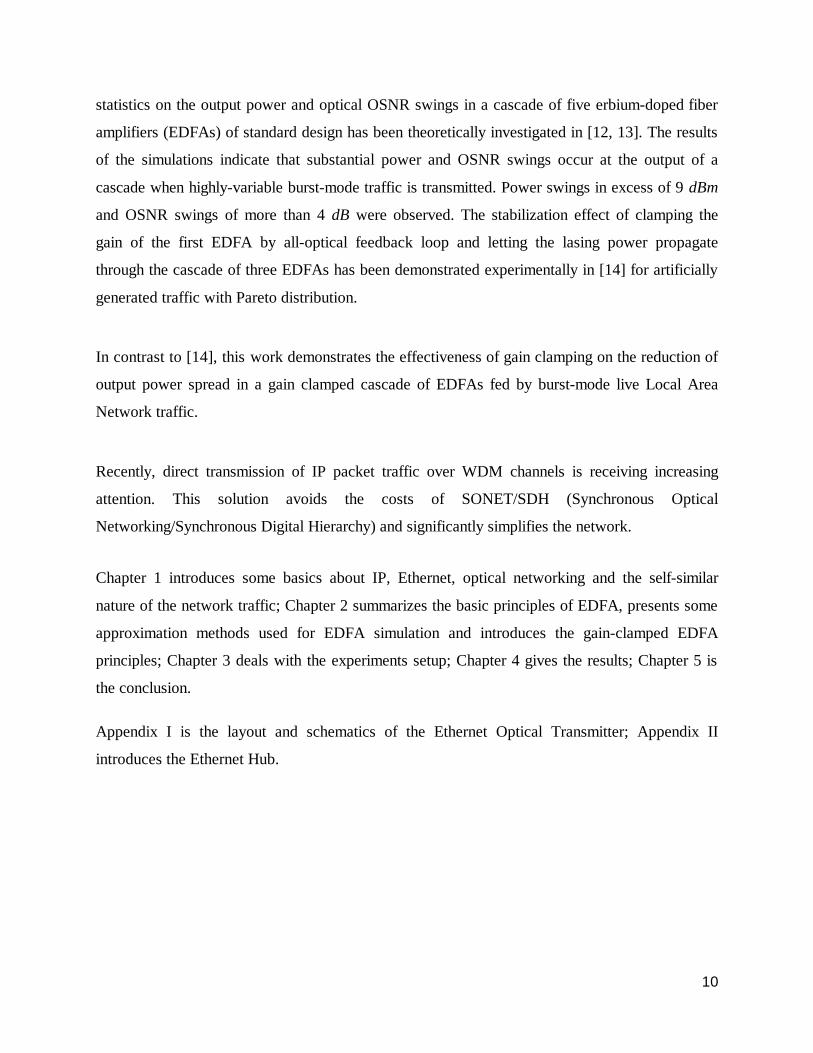
processing. This separation of networking function is called layering. For the OSI model, shown

in Figure 1-1, seven numbered layers indicate different functions.

12

Figure 1-1. The OSI model includes 7 layers that define network functionality

3. TCP/IP and Internet

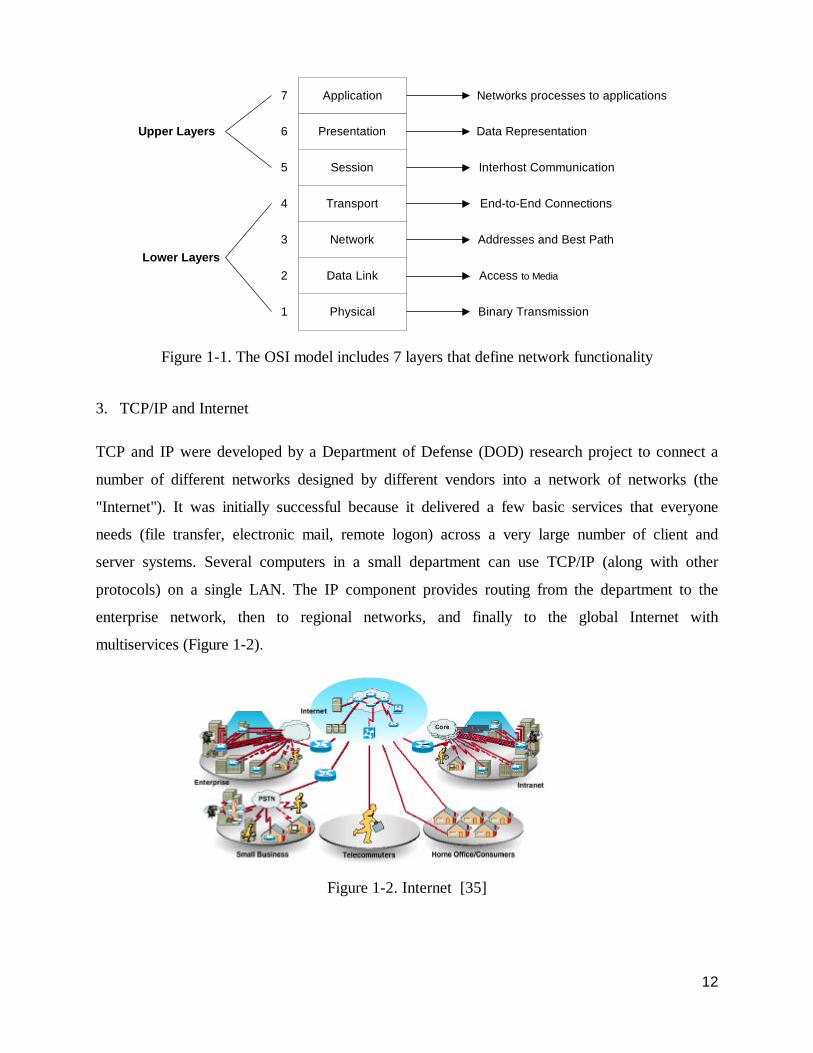
TCP and IP were developed by a Department of Defense (DOD) research project to connect a

number of different networks designed by different vendors into a network of networks (the

"Internet"). It was initially successful because it delivered a few basic services that everyone

needs (file transfer, electronic mail, remote logon) across a very large number of client and

server systems. Several computers in a small department can use TCP/IP (along with other

protocols) on a single LAN. The IP component provides routing from the department to the

enterprise network, then to regional networks, and finally to the global Internet with

multiservices (Figure 1-2).

Figure 1-2. Internet [35]

7

6

5

4

3

2

1

Networks processes to applications

Upper Layers

Lower Layers

Data Representation

Interhost Communication

End-to-End Connections

Addresses and Best Path

Access to Media

Binary Transmission

Application

Physical

Data Link

Network

Transport

Session

Presentation

13

The Internet is a system of linked networks that are worldwide in scope and facilitate data

communication services such as remote login, file transfer, electronic mail, the World Wide Web

and newsgroups.

With the meteoric rise in demand for connectivity, the Internet has become a communications

highway for millions of users. The Internet was initially restricted to military and academic

institutions, but now it is a full-fledged conduit for any and all forms of information and

commerce. Internet websites now provide personal, educational, political and economic

resources to every corner of the planet.

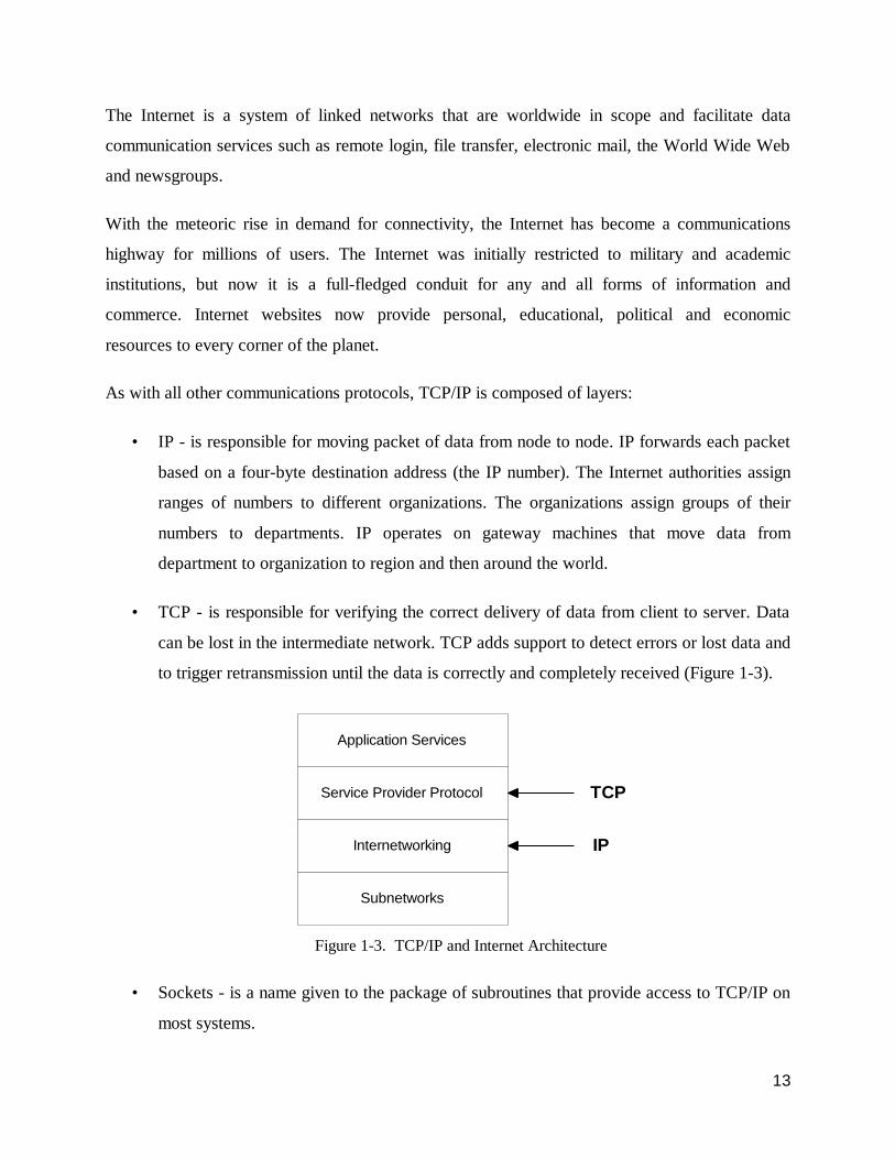
As with all other communications protocols, TCP/IP is composed of layers:

• IP - is responsible for moving packet of data from node to node. IP forwards each packet

based on a four-byte destination address (the IP number). The Internet authorities assign

ranges of numbers to different organizations. The organizations assign groups of their

numbers to departments. IP operates on gateway machines that move data from

department to organization to region and then around the world.

• TCP - is responsible for verifying the correct delivery of data from client to server. Data

can be lost in the intermediate network. TCP adds support to detect errors or lost data and

to trigger retransmission until the data is correctly and completely received (Figure 1-3).

Figure 1-3. TCP/IP and Internet Architecture

• Sockets - is a name given to the package of subroutines that provide access to TCP/IP on

most systems.

Application Services

Subnetworks

Internetworking

Service Provider Protocol TCP

IP

14

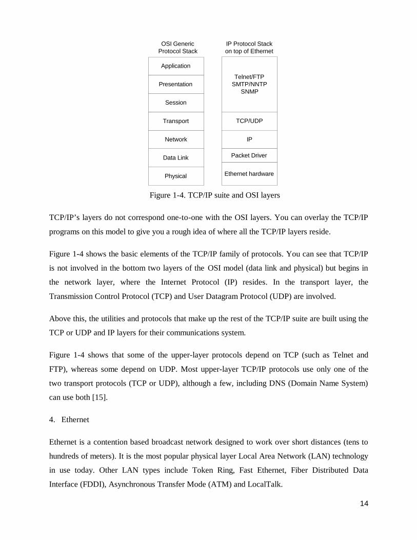
Figure 1-4. TCP/IP suite and OSI layers

TCP/IP’s layers do not correspond one-to-one with the OSI layers. You can overlay the TCP/IP

programs on this model to give you a rough idea of where all the TCP/IP layers reside.

Figure 1-4 shows the basic elements of the TCP/IP family of protocols. You can see that TCP/IP

is not involved in the bottom two layers of the OSI model (data link and physical) but begins in

the network layer, where the Internet Protocol (IP) resides. In the transport layer, the

Transmission Control Protocol (TCP) and User Datagram Protocol (UDP) are involved.

Above this, the utilities and protocols that make up the rest of the TCP/IP suite are built using the

TCP or UDP and IP layers for their communications system.

Figure 1-4 shows that some of the upper-layer protocols depend on TCP (such as Telnet and

FTP), whereas some depend on UDP. Most upper-layer TCP/IP protocols use only one of the

two transport protocols (TCP or UDP), although a few, including DNS (Domain Name System)

can use both [15].

4. Ethernet

Ethernet is a contention based broadcast network designed to work over short distances (tens to

hundreds of meters). It is the most popular physical layer Local Area Network (LAN) technology

in use today. Other LAN types include Token Ring, Fast Ethernet, Fiber Distributed Data

Interface (FDDI), Asynchronous Transfer Mode (ATM) and LocalTalk.

Application

Physical

Data Link

Network

Transport

Session

Presentation

OSI GenericProtocol Stack

Telnet/FTPSMTP/NNTP

SNMP

TCP/UDP

IP

Packet Driver

Ethernet hardware

IP Protocol Stackon top of Ethernet

15

Ethernet is popular because it strikes a good balance between speed, cost and ease of installation.

These benefits combined with wide acceptance in the computer marketplace and the ability to

support virtually all popular network protocols, make Ethernet an ideal networking technology

for most computer users today. The Institute for Electrical and Electronic Engineers (IEEE)

defines the Ethernet standard as IEEE Standard 802.3. This standard defines rules for

configuring an Ethernet network as well as specifying how elements in an Ethernet network

interact with one another. By adhering to the IEEE standard, network equipment and network

protocols can communicate efficiently.

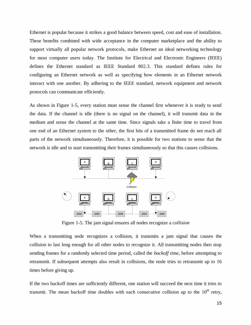
As shown in Figure 1-5, every station must sense the channel first whenever it is ready to send

the data. If the channel is idle (there is no signal on the channel), it will transmit data in the

medium and sense the channel at the same time. Since signals take a finite time to travel from

one end of an Ethernet system to the other, the first bits of a transmitted frame do not reach all

parts of the network simultaneously. Therefore, it is possible for two stations to sense that the

network is idle and to start transmitting their frames simultaneously so that this causes collisions.

Figure 1-5. The jam signal ensures all nodes recognize a collision

When a transmitting node recognizes a collision, it transmits a jam signal that causes the

collision to last long enough for all other nodes to recognize it. All transmitting nodes then stop

sending frames for a randomly selected time period, called the backoff time, before attempting to

retransmit. If subsequent attempts also result in collisions, the node tries to retransmit up to 16

times before giving up.

If the two backoff times are sufficiently different, one station will succeed the next time it tries to

transmit. The mean backoff time doubles with each consecutive collision up to the 10th retry,

A B C D

A B C D

JAM JAMJAMJAMJAM

Collision

16

thereby reducing the chance of collision in subsequent transmissions. From the 10th to the 16th

retry, the stations do not increase the backoff time any more but keep it constant [16, 17, 18].

High-Speed Ethernet Option

New applications can cause end users to experience delays and other troubles such as insufficient

bandwidth between end stations. In response to these problems, Ethernet networks have moved

forward with the availability of 100 Mbps technologies, such as:

• 100BaseFX--A 100 Mbps implementation of Ethernet over fiber-optic cable, the MAC layer

is compatible with the 802.3 MAC layer.

• 100BaseT4— A 100 Mbps implementation of Ethernet using 4-pair Category 3, 4, or 5

cabling, The MAC layer is compatible with the 802.3 MAC layer.

• 100BaseTX--A 100 Mbps implementation of Ethernet over Category 5 and Type 1 cabling.

The MAC layer is compatible with the 802.3 MAC layer.

• 100VG— Any LAN-The IEEE specification for 100Mbps implementation of Ethernet and

Token Ring over 4-pair UTP. The MAC layer is not compatible with the 802.3 MAC layer.

Figure 1-6. CSMA/CD Flow Chart

Increasing Ethernet bandwidth to 100 Mbps solves part of the bandwidth problem. Another part

of the solution is reducing the contention for the Ethernet media. One method of reducing

Station is ready to send

Wait according tobackoff strategy

(6)

Transmit succeed

Tranmit jam signal(5)

Transmit data & sensechannel

(4)

SenseChannel

(1)

New attempt

Channel Occupied(3)

No collision found

Channel available(2)

17

contention is built into Ethernet standard, namely the Carrier Sense Multiple Access with

Collision Detection (CSMA/CD) approach (Figure 1-6). A shared-media LAN must submit to

CSMA/CD so that no 2 users can simultaneously communicate over the shared LAN segment.

Switching also reduces contention for the media by creating multiple segments for desktop

devices and high-end applications (Figure 1-7). Switch in Figure 1-7 on the left splits the

Ethernet and thus reduces the number of users per shared segment. The switch makes multiple 10

Mbps or even 100 Mbps data pipes available. A limited number of users share a single 10 Mbps

or 100 bps segment. These users work in smaller collision domain with less contention from

other nodes. For users with high bandwidth needs and servers, one can provide a single dedicated

segment per user or server.

Figure 1-7. High-Speed Ethernet options and switching technologies offer more bandwidth to

users and workgroups

Coinciding with the rapid growth of high-speed Ethernet option is the deployment of ATM,

another high-speed technology.

Another high-speed technology is Gigabit Ethernet, or 1000BaseX. Gigabit Ethernet builds on

top of the Ethernet protocol but increases speed 10 times over fast Ethernet to 1000 Mbps, or 1

Gbps. This Media Access Control (MAC) and Physical Interface (PHY) standard, which was

approved on June 25, 1998, promises to be a dominant player in high-speed local-area network

(LAN) backbones and server connectivity. Customers will be able to leverage their existing

Ethernet knowledge base to manage and maintain Gigabit networks.

Switch

Router

18

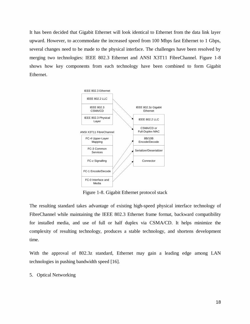
It has been decided that Gigabit Ethernet will look identical to Ethernet from the data link layer

upward. However, to accommodate the increased speed from 100 Mbps fast Ethernet to 1 Gbps,

several changes need to be made to the physical interface. The challenges have been resolved by

merging two technologies: IEEE 802.3 Ethernet and ANSI X3T11 FibreChannel. Figure 1-8

shows how key components from each technology have been combined to form Gigabit

Ethernet.

Figure 1-8. Gigabit Ethernet protocol stack

The resulting standard takes advantage of existing high-speed physical interface technology of

FibreChannel while maintaining the IEEE 802.3 Ethernet frame format, backward compatibility

for installed media, and use of full or half duplex via CSMA/CD. It helps minimize the

complexity of resulting technology, produces a stable technology, and shortens development

time.

With the approval of 802.3z standard, Ethernet may gain a leading edge among LAN

technologies in pushing bandwidth speed [16].

5. Optical Networking

IEEE 802.2 LLC

IEEE 802.3CSMA/CD

IEEE 802.3 PhysicalLayer

IEEE 802.3 Ethernet

FC-4 Upper-LayerMapping

FC-3 CommonServices

FC-z Signalling

FC-1 Encode/Decode

FC-0 Interface andMedia

ANSI X3T11 FibreChannel

IEEE 802.3z GigabitEthernet

IEEE 802.2 LLC

CSMA/CD orFull-Duplex MAC

8B/10BEncode/Decode

Serializer/Deserializer

Connector

19

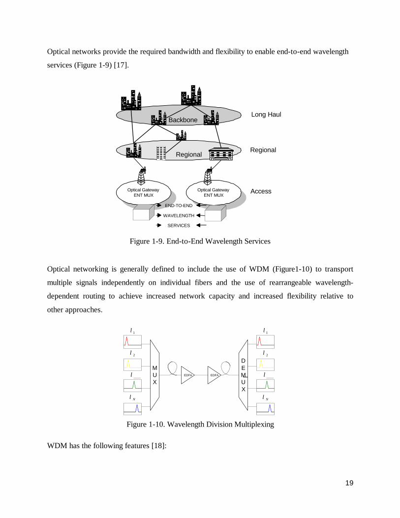
Optical networks provide the required bandwidth and flexibility to enable end-to-end wavelength

services (Figure 1-9) [17].

Figure 1-9. End-to-End Wavelength Services

Optical networking is generally defined to include the use of WDM (Figure1-10) to transport

multiple signals independently on individual fibers and the use of rearrangeable wavelength-

dependent routing to achieve increased network capacity and increased flexibility relative to

other approaches.

Figure 1-10. Wavelength Division Multiplexing

WDM has the following features [18]:

Optical GatewayENT MUX

Optical GatewayENT MUX

Long Haul

Regional

Access

END-TO-END

WAVELENGTH

SERVICES

Backbone

Regional

MUX

DEMUX

EDFA EDFA

1λ

2λ

........λ

Nλ

1λ

2λ

........λ

Nλ

20

• Multiplex multiple WDM channels from different users on the same fiber.

• The optical transmission spectrum is “carved-up” into a number of non-overlapping

wavelength (or frequency) bands, with each wavelength supporting a single communication

channel.

• The difference between electronics and optics is granularity (achieve rich connectivity

without a lot of optical connections. Electronics provide connectivity whereas optics provides

throughput).

Many factors are driving the need for optical networks. A few of the most important reasons for

migrating to the optical layer are described in this module.

• Fiber Capacity

The first implementation of what has emerged as the optical network began on routes that were

fiber limited. Providers needed more capacity between two sites, but higher bit rates or fiber

were not available. The only options in these situations were to install more fibers, which is an

expensive and labor-intensive chore, or place more time division multiplexed (TDM) signals on

the same fiber. WDM provided many virtual fibers on a single physical fiber. By transmitting

each signal at a different frequency, network providers could send many signals on one fiber just

as though they were each traveling on their own fiber.

• Restoration Capability

As network planners use more network elements to increase fiber capacity, a fiber cut can have

massive implications. In current electrical architectures, each network element performs its own

restoration. For a WDM system with many channels on a single fiber, a fiber cut would initiate

multiple failures, causing many independent systems to fail. By performing restoration in the

optical layer rather than the electrical layer, optical networks can perform protection switching

faster and more economically. Additionally, the optical layer can provide restoration in networks

that currently do not have a protection scheme. By implementing optical networks, providers can

add restoration capabilities to embedded asynchronous systems without first upgrading to an

electrical-protection scheme.

21

• Reduced Cost

In systems using only WDM, each location that demultiplexes signals will need an electrical

network element for each channel, even if no traffic is dropping at that site. By implementing an

optical network, only those wavelengths that add or drop traffic at a site need corresponding

electrical nodes. Other channels can simply pass through optically, which provides tremendous

cost savings in equipment and network management. In addition, performing space and

wavelength routing of traffic avoids the high cost of electronic cross-connects, and network

management is simplified.

• Wavelength Services

One of the great revenue-producing aspects of optical networks is the ability to resell bandwidth

rather than fiber. By maximizing capacity available on a fiber, service providers can improve

revenue by selling wavelengths, regardless of the data rate required. To customers, this service

provides the same bandwidth as a dedicated fiber.

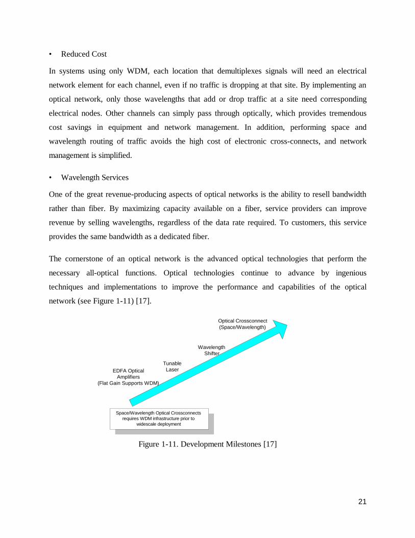
The cornerstone of an optical network is the advanced optical technologies that perform the

necessary all-optical functions. Optical technologies continue to advance by ingenious

techniques and implementations to improve the performance and capabilities of the optical

network (see Figure 1-11) [17].

Figure 1-11. Development Milestones [17]

EDFA OpticalAmplifiers

(Flat Gain Supports WDM)

Space/Wavelength Optical Crossconnectsrequires WDM infrastructure prior to

widescale deployment

TunableLaser

WavelengthShifter

Optical Crossconnect(Space/Wavelength)

22

Early Technologies

As fiber optics came into use, network providers soon found that some improvements in

technology could greatly increase capacity and reduce cost in existing networks. These early

technologies eventually led to the optical network as it is today.

• Broadband WDM

The first incarnation of WDM was broadband WDM. In 1994, by using fused biconic tapered

couplers, two signals could be combined on the same fiber. Because of limitations in the

technology, the signal frequencies had to be widely separated, and systems typically used 1,310-

nm and 1,550-nm signals, providing 5 Gbps on one fiber. Although the performance did not

compare to today's technologies, the couplers provided twice the bandwidth out of the same

fiber, which was a large cost savings compared to installing new fiber.

• Optical Fiber Amplifiers

The second basic technology, and perhaps the most fundamental to today's optical networks, was

the erbium-doped fiber amplifier. By doping a small strand of fiber with a rare earth metal, such

as erbium, optical signals could be amplified without converting the signal back to an electrical

state. The amplifier provided enormous cost savings over electrical regenerators, especially in

long-haul networks.

Erbium-doped Fiber Amplifier is the Key Enabling Technology for Optical Networking, as we

know its advantages for long-haul telecommunication:

• No O/E, E/O conversion - Amplify the optical signals in an optical medium => No

electronic bottleneck associated with electronic repeaters (which are complex,

expensive and provide no transparency).

• Larger bandwidth than electronic repeaters (up to 100 Gbps).

• Insensitive to bit rates.

• Transparent to modulation formats.

23

• Simultaneous regeneration of multiple WDM signals.

• Low cost and high reliability.

• Low noise, high gain.

• Very well suited for loss compensation of passive components in an optical

transmission system.

• Potential to create a universal lightpipe between terminals.

• Potential for high bit rate applications through WDM.

Erbium-Doped Fiber Amplifier can be used as (Figure 1-12):

• Power amplifiers at the transmitter.

• Optical pre-amplifiers in high bit-rate receivers.

• In line amplifiers to compensate loss in optical networks.

Figure 1-12. Usage of Erbium-doped Fiber Amplifier

Curent Technologies

Systems deployed today use devices that perform similar functions to earlier devices but are

much more efficient and precise. In particular, flat-gain optical amplifiers have been the true

enablers for optical networks by allowing the combination of many wavelengths across a single

fiber.

Tx RxEDFA EDFAEDFAEDFASMF

Power amp In-line amp In-line amp pre-amp

24

• Dense Wavelength Division Multiplexing (DWDM)

Figure 1-13. DWDM Systems

Figure 1-14. ITU channel spacing

As optical filters and laser technology improved, the ability to combine more than two signal

wavelengths on a fiber became a reality. Dense Wavelength Division Multiplexing (DWDM)

combines multiple signals on the same fiber, ranging up to 40 or 80 channels. By implementing

DWDM systems and optical amplifiers, networks can provide a variety of bit rates (i.e., OC–48

or OC–192), and a multitude of channels over a single fiber (see Figure 1-13). The wavelengths

used are all in the range that optical amplifiers perform optimally, typically from about 1,530 nm

to 1,565 nm (see Figure 1-14).

OC-48 OC-48

OC-48OC-48

OC-192OC-192

DWDM

DWDM

EDFA EDFAEDFA

25

Two basic types of DWDM are implemented today: unidirectional and bi-directional DWDM

(see Figure 1-15). In a unidirectional system, all the wavelengths travel in the same direction on

the fiber, while in a bi-directional system the signals are split into separate bands, with both

bands traveling in different directions.

Figure 1-15. Unidirectional and Bi-directional DWDM

• Optical Amplifiers

The performance of optical amplifiers has improved significantly— with current amplifiers

providing significantly lower noise and flatter gain— which is essential to DWDM systems. The

total power of amplifiers also has steadily increased, with amplifiers approaching +20–dBm

outputs, which is many orders of magnitude more powerful than the first amplifiers.

• Narrowband Lasers

Without a narrow, stable, and coherent light source, none of the optical components would be of

any value in the optical network. Advanced lasers with narrow bandwidths provide the narrow

wavelength source that is the individual channel in optical networks. Typically, long-haul

applications use externally modulated lasers, while shorter applications can use integrated laser

technologies.

26

Depending on the system used, the laser may be part of the DWDM system or embedded in the

SONET network element. When the precision laser is embedded in the SONET network

element, the system is called an embedded system. When the precision laser is part of the WDM

equipment in a module called a transponder, it is considered an open system because any low-

cost laser transmitter on the SONET network element can be used as input.

• Fiber Bragg Gratings

Figure 1-16. In-Fiber Bragg Grating Technology: Optical A/D Multiplexer [17]

Commercially available fiber Bragg gratings have been important components for enabling

WDM and optical networks. A fiber Bragg grating is a small section of fiber that has been

modified to create periodic changes in the index of refraction. Depending on the space between

the changes, a certain frequency of light— the Bragg resonance wavelength— is reflected back,

while all other wavelengths pass through (see Figure 1-16). The wavelength-specific properties

of the grating make fiber Bragg gratings useful in implementing optical add/drop multiplexers.

Bragg gratings also are being developed to aid in dispersion compensation and signal filtering as

well.

27

• Thin Film Substrates

Another essential technology for optical networks is the thin film substrate. By coating a thin

glass or polymer substrate with a thin interference film of dielectric material, the substrate can be

made to pass through only a specific wavelength and reflect all others. By integrating several of

these components, many optical network devices are created, including multiplexers,

demultiplexers, and add/drop devices.

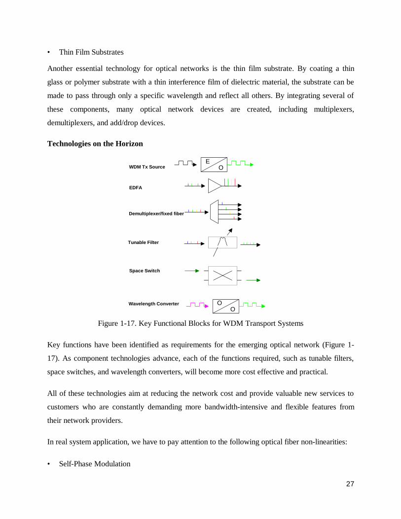
Technologies on the Horizon

Figure 1-17. Key Functional Blocks for WDM Transport Systems

Key functions have been identified as requirements for the emerging optical network (Figure 1-

17). As component technologies advance, each of the functions required, such as tunable filters,

space switches, and wavelength converters, will become more cost effective and practical.

All of these technologies aim at reducing the network cost and provide valuable new services to

customers who are constantly demanding more bandwidth-intensive and flexible features from

their network providers.

In real system application, we have to pay attention to the following optical fiber non-linearities:

• Self-Phase Modulation

WDM Tx Source

EDFA

Demultiplexer/fixed fiber

EO

OO

Tunable Filter

Space Switch

Wavelength Converter

28

• Cross-Phase Modulation

• Modulation Instability

• Four wave mixing

• Stimulated Brillouin Scattering

• Stimulated Raman Scattering

6. IP over WDM or DWWM

Figure 1-18. Network Bandwidth Prediction [19]

The amount of traffic— data, voice, and multimedia— traveling over the Internet and other

networks grows at rates that are hard to quantify, but everyone agrees the increase is beyond

anyone’s wildest dreams (Figure 1-18).

Once all this traffic leaves a local network (or home or small business), it goes into the hands of

a carrier or service provider, and typically is sent over a fiber optic cabling infrastructure. Even

service providers too small to have their own fiber infrastructure use fiber built and run by

someone else. Fiber optic cabling moves lots of traffic quickly, but even these fat pipes feel the

bandwidth pinch. So rather than pay exorbitant amounts to lay new fiber cabling, providers rely

on technologies that increase the amount of data a single piece of fiber can handle.

29

In order to still guarantee a high transmission speed, broadband communications networks with

optical fibers are employed.

By means of the WDM technology the potential for the transport capacity up to 1000 Gbit/s and

more on a single fiber is given. The WDM technology involves new requirements for the

network elements, which are therefore partially in research & development state. Depending on

the functionality of the WDM network elements, different network structures can be generated,

e.g. “broadcast and select”-networks or wavelength-routed networks.

Figure 1-19. IP Transport alternatives

In comparison to ATM, SONET and B-ISDN, the lower equipment and operational cost of

WDM also attracts more attention (Figure1-19) [19].

IP

ATM

SONET/SDH

Optical

IP

ATM

Optical

IP

SONET/SDH

Optical

IP

Optical

B-ISDN

IP overATM

IP overSONET/SDH

IP overWDM

Lower Equipment Cost & Operational Cost

30

IP over DWDM networks is shown in Figure 1-20. Multitechnologies coexist within one

network. DWDM can organize several different technologies including SDH/SONET, ATM and

IP into one network [20].

Figure 1-20. IP over DWDM

7. Self-similar Nature of the packetized traffic

Self-similar process was considered in modeling cell traffic in modern communication networks,

in particular, telecommunication traffic in high-resolution Ethernet local area networks, wide-

area networks, and also for variable-bit-rate video traffic. This was motivated by experimentally

observed long-range dependence of traffic data and “burstiness” of traffic streams across an

extremely wide range of time scales [9, 10, 21].

A process is said to be self-similar when it exhibits correlation at all time lags. For instance

packet of network traffic looks the same when measured over time scales ranging from seconds

to minutes and hours, and it can be well modeled as having a heavy-tailed distribution. W.

Leland et al recorded Ethernet traffic of Bellcore for 27 hours [21]. Figure 1-21 shows plots of

the packet counts (number of packets/time unit) for 5 different time scales. Traffic “spikes” ride

on longer-term “ripples”, that in turn ride on still longer term “swells”. This graphic proof of the

self-similar nature of Ethernet traffic illustrates the statistical identity between Ethernet traffic on

one time scale and on a different time scale.

A self-similar process has a distribution that is heavy-tailed, i.e. its distribution follows a power

law asymptotically. That is,

∞→> − xxxXP as~][ α

EDFA

MU

XD

EM

UX

Traditional SONET ADMSONET ADM

IP

IP

IP

IP

ATM SONET ADMSONET ADM

SONET ADMSONET ADM

TxT

TxT

TxT

TxT

TraditionalSONET ADMSONET ADM

IP

IP

IP

IP

ATMSONET ADMSONET ADM

SONET ADMSONET ADM

RxT

RxT

RxT

RxTPhotonic Layer Protection

IP Recovery withoutPhotonic Layer Protection

31

where 0<α<2. One of the simplest heavy-tailed distributions is the Pareto distribution whose

probability density function is given by

where α is the shape parameter, and k is the location parameter. Its distribution function has the

following form

Figure 1-21 (a)-(e). Pictorial Proof of Self-Similarity: Ethernet Traffic on 5 different time scales

(Different gray levels are used to identify the same segments of traffic on the different time scales) [10]

Heavy-tailed distributions have a number of properties that are qualitatively different from

distributions more commonly encountered in network research, particularly, the exponential

distribution. If a = 2, the distribution has infinite variance, and if a = 1, the distribution has also

infinite mean. Thus, as a decreases, a large portion of the probability mass resides in the tail of

the distribution.

kxkxkxp ≥>= −− 0)( 1ααα

α

−=≤=

xkxXPxF 1][)(

32

The overall network utilization is given as ][][

][

offon

on

TETETE+

=ρ . When we know the utilization or

network load ρ and the mean of the ON periods ][ onTE , the offα parameter can be related to onα

by [13]

)1()1()1(

−−−−=

onon

onoff αραρ

αρα

Another quantitative measure of self-similarity is obtained by using Hurst parameter H [10],

which expresses the speed of decay of a time series’ autocorrelation function. As mentioned

earlier, a time series with long-range dependence has an autocorrelation of the form

Where 0<ß<1. Hence, when compared to the exponential decay exhibited by traditional traffic

models, the autocorrelation function of a long-range dependent process decays according to a

power-law. The Hurst parameters is related to ß via H=1- ß/2. So, for self-similar time series,

½<H<1. As H? 1, the degree of self-similarity increases. A test for self-similarity of a time

series can be reduced to the question of determining whether H significantly deviates from ½.

Traditional network traffic is modeled by Poisson processes, which become smoother as you

observe their behavior over longer time intervals. Self-similar renewal processes do not smooth

so that they are invariant with respect to the time period over which you observe them. Such

behavior has serious consequences when applied to traffic models since it indicates that you will

always get bursts of traffic at every time scale and you can never allocate enough queuing

resources to handle every situation [22].

In [12,13,14] the response of EDFAs to self–similar traffic was examined. This type of traffic

has a dramatic effect on gain transients and motivated the experimental work presented in later

chapters.

∞→− kkkr as~)( β

33

Chapter 2. Erbium-Doped Fiber Amplifier (EDFA)

Introduction

An alternative to optoelectronic regenerators has appeared in the last decade due to the discovery

of optical fiber amplifiers, notably the erbium-doped fiber amplifiers for the 1500 nm

communications band. These were first reported in 1987 to amplify optical signals directly and

thus make all-optical communication systems possible.

Erbium-doped fiber amplifiers are now widely used in long haul communication systems to

boost the signals. It is safe to say that, starting in 1989, erbium-doped fiber amplifiers were the

catalysts for an entirely new generation of high-capacity undersea and terrestrial fiber-optic links

and networks. EDFAs also reinvigorated the study of optical solitons for fiber-optic

transmission, since they now made practical the long distance transmission of solitons.

EDFA have been widely applied in optical networks as they have many unique properties which

are suited for optical communications [23, 24, 25], such as:

• They operate in the telecommunication wavelength band of 1530-1610 nm with high gain,

(Small signal gain > 40 dB), high output power (P > 100 mW) and low noise.

• High-power semiconductor laser diodes are practical sources to provide the light to pump

EDFAs.

• The EDFA is fiber compatible and can be spliced into transmission fibers with less than one

dB of insertion loss.

• The gain of EDFAs is unaffected by signal polarization.

• Because saturation occurs in EDFAs on such a slow time scale (~10 msec), EDFAs are

relatively immune to crosstalk among wavelength multiplexed channels or pulse distortion in

high-bit-rate systems.

34

EDFAs are developing so rapidly that they are soon expected to replace the optoelectronic

repeaters in many existing applications such as power amplifiers to boost transmitter power,

optical repeaters to amplify weak signals and optical preamplifiers to increase receiver

sensitivity.

Typical application of EDFA in point to point transmission systems and distribution systems is

shown in Figure 2-1.

Figure 2-1 (a) Amplifiers in point to point transmission system

(b) Amplifiers in networks

Tx RxEDFA EDFA EDFA

Power amp Repeater Preamp

(a)

(b)

Switch

EDFA

EDFA

EDFA

35

1. Basic EDFA Configuration

An EDFA consists of a short length of optical fiber (usually less than about 100 m) whose core

has been doped with less than 0.1 percent erbium, an optically active rare earth element that has

many unique intrinsic properties for optical amplification. For example, the erbium atom has a

metastable state with the remarkable long lifetime of 10 ms. This makes it possible to obtain an

optical gain which takes a long time to saturate.

Figure 2-2 shows the construction of a typical EDFA module. The erbium-doped fiber (EDF) is

compatible with conventional fiber and may be fusion spliced to other components. The pump

light is combined with the incoming signal by using a wavelength division multiplexer. Pump

light propagating along the EDF is depleted as erbium ions are raised to an excited state. As the

signal propagates in the EDF, it stimulates emission of light from the excited ions, thereby

amplifying the signal power.

Figure 2-2. Basic EDFA configuration

Currently an EDFA is constructed by fusion splicing discrete fiber-pigtailed components. It

mainly consists of an erbium-doped fiber, a wavelength division multiplexer and a pump light

source. In addition, a polarization insensitive optical isolator or an optical bandpass filter is

required to improve EDFA performance. The optical isolator is used to achieve stable amplifier

Signalout

EDFA

Isolator Filter

Signalin

Pump

WDM

36

operation (it prevents spurious oscillations). The filter is used to greatly reduce the amplified

spontaneous emission (ASE) and to protect the amplifier from saturation caused by ASE

accumulated in the in-line amplifier system. Care should be taken in applying isolators to EDFAs

in LANs. For example, we can’t use typical isolators in LANs with the star topology when the

signals are bi-directional. One solution is to keep the gain of EDFA small enough (around 15 dB)

to avoid using isolators.

In order to pump the erbium ions up to an upper energy level, there are several proper pump

wavelength bands. At present, 1480 nm and 980 nm high power laser diodes have proved to be

the two most efficient pump wavelengths.

In practice, there are three basic EDFA configurations. They are classified mainly according to

their pump light propagation direction. In forward pumping, the signal light copropagates with

the pump light whereas in backward pumping it counter-propagates relative to the pump light.

From the viewpoint of noise performance, forward may be more profitable [26]. On the other

hand, backward pumping may be effective for high-power output. In addition, one can have bi-

directional pumping with pump power traveling simultaneously in both directions.

37

2. Saleh and Sun’s Model

In this section we present a model of the amplification process of an EDFA, as described by

Saleh et al in [28]. As seen in Figure 2-3, the erbium ions in the EDFA can occupy one of these

states with increasing energy: the ground state ( 2/154I ), the metastable state ( 2/13

4I ), the excited

state ( 2/114I ).

Figure 2-3. Erbium Energy Level

First let’s introduce some symbols to describe a 2-level Er3+-doped fiber system (Figure 2-3.)

Table 2-1. EDFA parameters

the fraction of ions excited on metastable level N2 [0≤ N2≤1] the photon flux Qk [photons/s] the channels k, k=0… N metastable level lifetime τ [s] Er3+ ion density ρ [m-3] fiber core effective area A [m2] confinement factor of channel k Γk the emission cross-section of channel k σk

e [m2] the absorption cross-section of channel k σk

a [m2] σk

T=σke+σk

a the length of the Er3+ doped fiber L [m]

direction sign uk=l 11

0−

==

entering atentering at

zz L

38

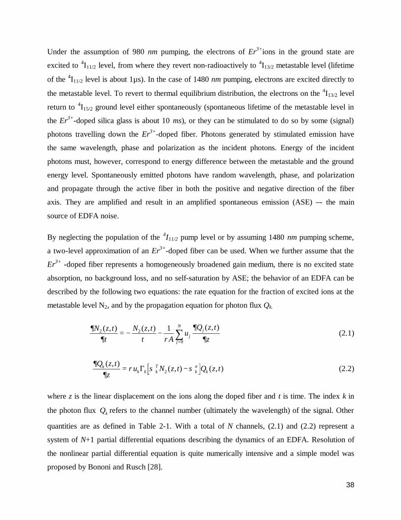
Under the assumption of 980 nm pumping, the electrons of Er3+ions in the ground state are

excited to 4I11/2 level, from where they revert non-radioactively to 4I13/2 metastable level (lifetime

of the 4I11/2 level is about 1µs). In the case of 1480 nm pumping, electrons are excited directly to

the metastable level. To revert to thermal equilibrium distribution, the electrons on the 4I13/2 level

return to 4I15/2 ground level either spontaneously (spontaneous lifetime of the metastable level in

the Er3+-doped silica glass is about 10 ms), or they can be stimulated to do so by some (signal)

photons travelling down the Er3+-doped fiber. Photons generated by stimulated emission have

the same wavelength, phase and polarization as the incident photons. Energy of the incident

photons must, however, correspond to energy difference between the metastable and the ground

energy level. Spontaneously emitted photons have random wavelength, phase, and polarization

and propagate through the active fiber in both the positive and negative direction of the fiber

axis. They are amplified and result in an amplified spontaneous emission (ASE) –- the main

source of EDFA noise.

By neglecting the population of the 4I11/2 pump level or by assuming 1480 nm pumping scheme,

a two-level approximation of an Er3+-doped fiber can be used. When we further assume that the

Er3+ -doped fiber represents a homogeneously broadened gain medium, there is no excited state

absorption, no background loss, and no self-saturation by ASE; the behavior of an EDFA can be

described by the following two equations: the rate equation for the fraction of excited ions at the

metastable level N2, and by the propagation equation for photon flux Qk.

∂∂ τ ρ

∂∂

N z tt

N z tA

uQ z t

zjj

j

N2 2

0

1( , ) ( , ) ( , )= − −

=∑ (2.1)

∂∂

ρ σ σQ z tz

u N z t Q z tkk k k

Tka

k( , )

( , ) ( , )= −Γ 2 (2.2)

where z is the linear displacement on the ions along the doped fiber and t is time. The index k in

the photon flux kQ refers to the channel number (ultimately the wavelength) of the signal. Other

quantities are as defined in Table 2-1. With a total of N channels, (2.1) and (2.2) represent a

system of N+1 partial differential equations describing the dynamics of an EDFA. Resolution of

the nonlinear partial differential equation is quite numerically intensive and a simple model was

proposed by Bononi and Rusch [28].

39

3. Bononi and Rusch’s Reservoir model

If we make some transformations to (2.1, 2.2), we can achieve Bononi and Rusch’s Reservoir

model:

Dividing both sides of (2.2) by Qk ≠ 0 , multiplying by dz and integrating from z=0 to L we

obtain

G t B r t Ak k k( ) ( )= − , k=0,......,N (2.3)

where

])()(

ln[0 tQ

tQQ

QuG in

k

outkL

k

kkk == ∫ ∂

(logarithmic gain) (2.4)

and A Lk k ka= ρ σΓ and B

Akk k

T

= Γσ are non-dimensional parameters.

Multiplying (2.1) by dz, integrating along the fiber axis from z=0 to L and substituting for Qkout

from (2.4), a single first order ordinary differential equation (ODE) is obtained, which describes

the time evolution of the length averaged metastable level population r(t)

∑=

−−+=N

j

AtrBinj

jjetQtr

trdtd

0

)( )1)(()(

)(τ

(2.5)

where r(t), the “reservoir”, represents the total number of excited ions in the amplifiers:

r t A N z t dzL

( ) ( , )= ∫ρ 20 max)(0 rtr << (rmax=ρAL is the total number of ions in the doped fiber).

When normalizing the state variable r(t) to rmax , a first order ODE for the normalized reservoir

x tL

N z t dz r trM

L( ) ( , ) ( )= =∫1

20 can be derived

40

∑=

−Γ−+−=N

j

txLinj a

kTkke

ALtQtx

txdtd

0

))(( )1()()(

)( σσρ

ρτ (2.6)

The reservoir model can be understood clearly by the following figure:

Figure 2-4. Reservoir model

Excited ions are represented by “water” in the reservoir. The pump fills the reservoir, except for

some leakage due to fluorescence. As signals enter from the left and exit to the right they draw

off ions from the reservoir and experience a wavelength dependent gain which varies with the

level of the reservoir.

Note that the set of 1+N coupled nonlinear partial differential equations in (2.1) and (2.2) have

been reduced to a single nonlinear ordinary differential equation in (2.5) vastly simplifying

simulation. The equation can be further simplified under certain conditions as described in the

next section.

41

4. Approximate Solutions

The Reservoir model is convenient to calculate the EDFA gain transient, which is caused by

1. network reconfiguration;

2. periodic addition/removal of channels or network failures;

3. sudden loss of many channels.

Numerical solution to the ODE (2.5) or (2.6) for an analysis of concatenated EDFAs may be

rather time consuming when packetized bursty traffic is considered. Further linearization of the

numerical problem is necessary to make the numerical calculations easier and faster.

Two separate approximations of the models presented have been proposed. Both approximations

lead to a exponential model for reservoir and gain, but with differing exponential time constants.

We develop these approximations here in order to compare and contrast results.

• Bononi & Rusch’s method [28]

We start from a small signal solution and use exponential approximation.

For small t, we use

))0()(())0()(( rtrBe krtrBk −≈− (2.7)

So the ODE solution of (2.5) yields

)1)(0(')0()( / ete errtr ττ −+ −+= (2.8)

where )0(' +r is the time derivative of the reservoir just after time t=0.

Suppose that the solution is of the form

etYeXtr τ/)( −+=

We force r(0), r(∞ ) and r’(0) to follow this, so

42

eterrrtr τ/)]()0([)()( −∞−+∞= (2.9)

where )0('

)0()(+

−∞=r

rreτ follows from these assumptions.

• Sun et al’s Approximation [27]

Start from the following:

])(exp[)( 000 tgLgLgQtQ nnninn

outn ∆+= (2.10)

where

=

)()(1

)(tQtQ

InL

tg inn

outn

n is the average exponential gain

We can easily get

)/exp(

)()0(

)()(τt

outn

outnout

noutn Q

QQtQ

−

∞∞= (2.11)

where

∑=

+=

N

iISi

outi

QQ

1

0

0

1

ττ , QiIS is each channel’s saturation photon flux

• Transforming Bononi’s solution to Sun’s

According to our Reservoir model, the gain is

kkk AtrBtG −= )()(

And the output is

)()()( tGnk

outk

ketQtQ =

The approximation is

eterrrtr τ/)]()0([)()( −∞−+∞≈ (2.12)

43

SSr (8 ) is the steady state of r.

We go further

)/exp(

/

)()0(

)()]()0([)(exp)(e

e

t

outk

outkout

kktSS

kSS

kink

outk Q

QQAerrBrBtQQ

ττ

−−

∞∞=−∞−+∞= (2.13)

We can see that reservoir approach gives the same form as Sun’s method; it just differs in τ.

In the next section we present simulation results for these two approximations which differ only

in the exponential time constant.

Figure 2-5. A simple WDM system

Figure 2-5 shows a simple WDM system. We will use our Reservoir model to simulate the

surviving channel (Channel 1)’s power excursion and the change of Reservoir when 7 channels

are added/dropped, and also when 4 channels are dropped.

Our simulation actually supposes that the EDFA has two input channels =1CHλ 1552.4 nm and

=2CHλ 1557.9 nm, with initial input powers =1CHP -2 dBm, =2CHP -2+10 )7(log10 dBm,

simulating the remaining 7 channels of an eight-channel system with –2 dBm/channel. EDFA is

pumped at 980 nm, =pumpP 18.4 dBm, L=35 m, t=10.5 ms. The absorption coefficients are

[0.257, 0.145, 0.125] 1m − and the intrinsic saturation powers are [0.440, 0.197, 0.214] mW at

[980, 1552.4, 1557.9] nm, respectively. The system is at equilibrium before t=0. At t=0 part of

the power on channel 2 is dropped, simulating the drop of a given number channels [28].

MU

XD

EM

UX

EDFA

CH1

CH2

CH1

CH2

CH3 CH3

CH8

CH7CH7

CH6CH6

CH5CH5

CH4CH4

CH8

44

Figure 2-6. Add/Drop simulation using Reservoir model

Figure 2-6 shows the dynamics of the Reservoir and output power excursion of channel 1

defined as ])0(

)([log10

1

110 +out

out

QtQ .

Figure 2-7. Our Add/Drop Experiment

Figure 2-7 is our Add/Drop experiment result measured by the photodetector, the vertical axis

stands for the output from the surviving channel 1 in dB scale. We can see that the responses of

the channel 1 to other channel’s add/drop have the same trends as our simulation, and it shows

that our reservoir model is correct to model the real add/drop situations.

0 20 40 60 80 100 120 140 160 180 1.1 1.2 1.3 1.4 1.5 x 10 14

Time (us)

Res

ervo

ir

7 ch add

7 ch drop

4 ch drop

0 20 40 60 80 100 120 140 160 180 -10 -5 0 5

10

Ch

1 P

ower

Exc

ursi

on (

dB)

Time (us)

7 ch add

7 ch drop 4 ch drop

0 20 40 60 80 100 120 140 160 180 200 -8

-7

-6

-5

-4

-3

-2

-1

0

1

PD

Out

put (

dBV

)

Time (10 us)

Channel Add Channel Add

Channel Drop Channel Drop

45

• Sun et al’s experimental results.

Figure 2-8. Sun’s results [29]

We can compare Figure 2-7 and Figure 2-8 (a) and see the same exponential rise (after a drop)

and exponential decay (after an add). Furthermore, in Figure 2-8 (b), Sun et al fit their data to an

exponential curve, but with the time constant determined numerically, not using equation (2.11).

In the next section we explain three simulations:

1). Bononi time constant--- equation (2.9)

2). Sun’s time constant---equation (2.11)

3). Numerical fit to the time constant

We compare the exact solution, exponential approximation and Sun’s method (Figure 2-9.), from

which we can see that Bononi’s exponential approximation is closer to the real case and hence is

better. It fits well in the small signal region, when t grows, it differs more from the real solution,

but as t tends to infinity, it converges to the real case again. When there is less change, the

difference between the exact solution and the approximation is smaller, but when the add/drop is

bigger, the difference is more evident.

46

Figure 2-9. Real case and approximations

• Our fit method

We can see that the EDFA gain dynamics has an exponential trend, which gives us some

intuition to make some exponential fit. But we can see it is not ideal in the small t region, so we

make a linear fit for small t, while putting an exponential fit for larger t, and it works well in both

7 and 4 channels data cases (Figure 2-10).

Figure 2-10. Some fit methods

0 20 40 60 80 100 120 140 160 180 2001.1

1.15

1.2

1.25

1.3

1.35

1.4x 10

14

Time (us)

7 channels data

Exact SolutionBononi (taue=93.49 us)Sun (taue=202.18 us)Exponential Fit (taue=63.88 us)Small Linear FitMiddle Expo Fit (taue=56.57 us)

0 20 40 60 80 100 120 140 160 180 2001.14

1.15

1.16

1.17

1.18

1.19

1.2

1.21

1.22

1.23

1.24x 10

14

Time (us)

4 channels data

Exact SolutionBononi (taue=63.04 us)Sun (taue=83.03 us)Exponential Fit (taue=53.03 us)Small Linear FitMiddle Expo Fit (taue=50.74 us)

0 20 40 60 80 100 120 140 160 180 2000

0.5

1

1.5

2

2.5

3x 10

17

Pow

er (p

hoto

ns)

Time (us)

1 Channel Drop

4 Channels Drop

7 Channels Drop

Exact Solution BononiSun

47

5. EDFA Cascade

A serious problem facing wavelength division multiplexed networks with fiber amplifier

cascades is transient cross saturation or gain dynamics of fiber amplifiers. Attention has been

focused primarily on circuit-switched scenarios. When the number of WDM channels

transmitted through a circuit-switching network varies, channel addition/removal will tend to

perturb signals at the surviving channels that share all or part of the route. Power transients in the

surviving channels can cause severe service impairment due to either inadequate eye opening or

the appearance of optical nonlinear ties [1].

Signal power excursions more serious than those induced by channel addition/removal in circuit

switched networks can arise when data on the WDM channels is highly variable in nature. Self-

similar traffic can lead to large variation in EDFA gain.

When self-similar packet traffic is directly transmitted in burst-mode on the WDM channels, as

in the case of Internet Protocol (IP) over WDM, long inter-burst idle intervals may give enough

time to fiber amplifiers to reach gains greatly exceeding the average values. This can in turn lead

to significant variation in output power and optical OSNR. This effect accumulates along a

cascade of fiber amplifiers in the same way as the fast power transients in the circuit-switching

scenario. The effect of WDM traffic statistics on the output power and OSNR swings in a

cascade of five EDFAs of standard design has been theoretically investigated in [31, 32]. The

results of the simulations indicate that substantial power and OSNR swings occur at the output of

a cascade when highly variable burst-mode traffic is transmitted. Power swings in excess of 9 dB

and OSNR swings of more than 4 dB were observed. The stabilization effect of clamping the

gain of the first EDFA by all-optical feedback loop and letting the lasing power propagate

through the cascade of six EDFAs has been studied in [33].

In order to prevent unacceptable error burst, the channel power should be maintained constant.

EDFAs for WDM systems do not have a very flat gain-wavelength figure (Figure 2-13), which

also tremendously varies due to saturation when the input power is large. In the design of

optically amplified links for WDM application, in which the number and the power level of the

input channels may vary randomly in time as in a packet switched scenario, it is thus important

48

to stabilize the EDFA’s gain profile. Gain-clamped EDFA can stabilize the average inversion

and thus clamp the gain to the desired level, which also motivates our measurements of cascades.

Our results show that output power and OSNR swings can be effectively suppressed if the first

amplifier of the cascade is gain clamped using an all-optical feedback loop and the lasing power

generated in the gain clamped EDFA propagates along the cascade.

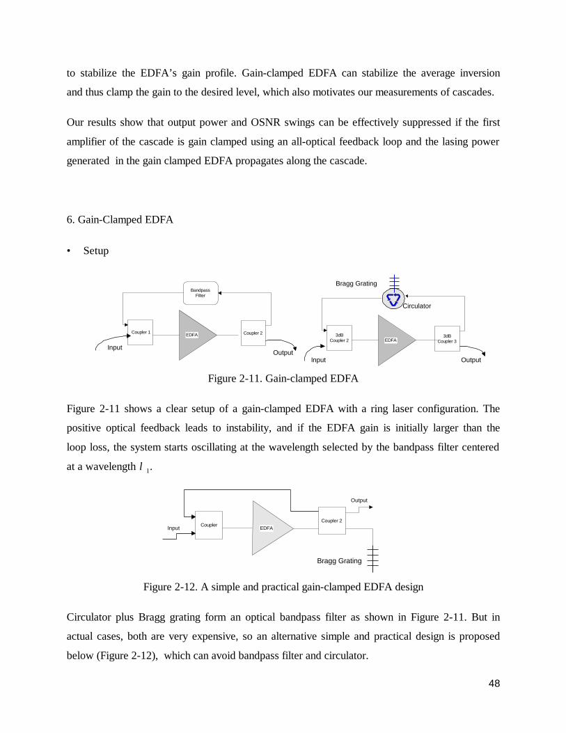
6. Gain-Clamped EDFA

• Setup

Figure 2-11. Gain-clamped EDFA

Figure 2-11 shows a clear setup of a gain-clamped EDFA with a ring laser configuration. The

positive optical feedback leads to instability, and if the EDFA gain is initially larger than the

loop loss, the system starts oscillating at the wavelength selected by the bandpass filter centered

at a wavelength λ1.

Figure 2-12. A simple and practical gain-clamped EDFA design

Circulator plus Bragg grating form an optical bandpass filter as shown in Figure 2-11. But in

actual cases, both are very expensive, so an alternative simple and practical design is proposed

below (Figure 2-12), which can avoid bandpass filter and circulator.

CouplerCoupler 2

EDFA

Bragg Grating

Output

Input

3dBCoupler 2

3dBCoupler 3EDFA

Bragg Grating

Circulator

Input Output

Coupler 1 Coupler 2EDFA

BandpassFilter

InputOutput

49

• Analysis

We assume that the erbium ion has two energy levels and a homogeneously broadened gain

spectrum. We can get a new equation, taking into account the self-saturation induced by the

amplified spontaneous emission (ASE), so (2.5) is updated to

))(()()]([1)()(,,

trQtrtrGtQtrdtd

ASElpSj

jj −−−= ∑∈ τ

(2.14)

where Q r tASE ( ( )) is the ASE flux

When considering the optical feedback, we just let the laser input flux as a delayed and

attenuated version of the output flux, to which the ASE term Ql ASE, passed by the feedback filter

is added

)]([)]([)()( , lASElllll trQtrGtQtQ τττα −+−−= (2.15)

τ l is the loop propagation delay and 10 ≤≤α the loop attenuation, both at laser wavelength λl .

Equation (2.14) and (2.15) form the model of the gain-clamped EDFA. There are now 2

variables, the other is the laser flux Q tl ( ) .

In [30], Bononi et al analyzed these equations, and produced the curves shown in Figure 2-13.

Figure 2-13. Gain versus average inversion and wavelength [30]

50

According to equation (2.3), the gain in dB is

)(34.4log10)(log10 1010 jjjjArB ArBeArBe jj −=−=−

We plot the gain against wavelength, and inversion that is maxrrx = . For a fixed value of the

reservoir r, or the equivalent x, we have the well-known gain-wavelength profile. The variation

of x caused by the input power variation causes the undesirable profile changes. The gain has a

linear dependence on r.

The loop filter passes only wavelength lλ , i.e., chooses the straight line corresponding to the

laser gain shown on the surface (Figure 2-13). The horizontal contour line on the surface marks

the level corresponding to the loop loss at wavelength lλ (the loop loss at all other wavelengths

is infinity). The laser flux grows till its gain equals the loop loss, thus fixing the inversion and the

gain to a desired value. The desired inversion can be changed by either changing the loop loss for

fixed lλ (thus moving along the laser gain line), or by changing lλ for fixed loss (thus moving

along the loop loss contour).

The equilibrium point at the intersection of the loop loss contour and the laser gain line is stable.

Actually, if some channels are dropped, less reservoir ions are consumed, x tends to increase, and

so does the laser gain and the laser flux, which grows to consume the excess reservoir ions and

brings x back to its clamped value. If some channels are added, more reservoir ions are

consumed, x tends to decrease, and so does the laser gain and the laser flux, which costs less

reservoir ions and bring x back to its clamped level.

51

8. Cross-Gain Modulation

Figure 2-14. Setup

Gain-clamped EDFA is very effective in suppressing the surviving channel’s output excursion in

the Add/Drop scenario. In order to measure these effects, we assembled an experimental setup.

According to the setup of Figure 2-14, one channel is modulated by a square wave at 1 kHz to

simulate Add/Drop, and another probe channel is a CW channel that stands for the surviving

channel. We observe the CW channel’s output.

Figure 2-15. Cross gain modulation

1k Hzmodulated

signal1550nm

3dBCoupler 1

CW Laser1555.08nm

3dBCoupler 2

3dBCoupler 3

EDFA

Filter 1560 nm

PhotoDetector

Data Acquisition

Brag Grating 1555.08nm

Circulator

0 500 1000 1500 2000 2500 3000 3500 4000 4500 5000 2

4

6

8

10

Time (2.5 us)

PD

Out

put (

V)

Crossgain Modulation for Low Frequency(1 kHz) Unclamped Clamped

2 3 4 5 6 7 8 9 10 -6

10 -4

10 -2

10 0

PD

F

PD Output (V)

Unclamped Clamped

52

We see from Figure 2-15 that, the CW channel is also modulated, which is called cross-gain

modulation, while under gain-clamped circumstances, the amplitude of the modulation are

reduced greatly, from 4 V to 0.2 V. The lower plot is the Probability Density Function (PDF) of

the output; we will also discuss this later in Chapter 4.

The cross-gain modulation just occurs in the kHz range. When we repeat the experiment above

while raising the frequency up to hundreds of kHz, cross-gain modulation disappears.

53

Chapter 3. Experimental Setup

In this chapter we provide a detailed description of the experimental setup used to measure the

dynamic response of EDFAs to live Ethernet traffic that is self-similar in nature. In Chapter 4 we

will examine experimental results.

1. General Setup

Our experimental setup is shown in Figure 3-1. Electrical signal from the Ethernet Hub----

CenterCOM MR820TR for 10 Mbps (Appendix II) which carries all traffic of the LAN is

converted by an Ethernet transmitter to optical signal and fed into the gain-clamped (when the

toggle T is on) or unclamped (when the toggle T is off) EDFAs cascade. We used Corning Gain

Module EDFAs concatenated with five 20dB fiber attenuators that represent the loss of

transmission fibers.

3dB Coupler 1

CW Laser 1556.27nm

3dB Coupler 2

3dB Coupler 3

EDFA

Live Ethernet Data at 10 Mb/s

(Electrical Signals)

Ethernet Transmitter 1550nm

(Optical Signal) T

EDFA EDFA ATTN ATTN

Photo Detector

Data Acquisition

Bragg Grating 1556.27nm

Circulator

Bandpass Filter 1560 nm

Variable Attenuator

Figure 3-1. Experiment Setup

54

In order to monitor the effect of cross gain saturation in individual EDFAs on the bursty LAN

traffic, a CW signal at 1556.27nm is introduced at the input of the EDFA coupled via a 3dB

directional coupler. The Ethernet optical transmitter (1550nm) is used to represent several

channels of a WDM system. Therefore, the average power of this signal channel at the input

port of the EDFA was set to –13dBm and the power of the CW monitoring channel was set at

20dBm. Power fluctuations in the CW signal represent changes in the inversion level (or

Reservoir) and hence reflect gain variation of the EDFA. The power of the CW channel at the

output of the individual EDFAs along the cascade caused by bursty Ethernet traffic are

detected after filtering out this signal channel using an optical band pass filter (JDS-Fitel

CR2500 circulator with a Bragg grating at 1556.27 nm). The electrical signal from the ANTEL

ARX-GP photodetector is processed in a National Instrument’s PCI6110-E data acquisition

card inside a PC.

2. Ethernet Optical Transmitter

The block diagram of the Ethernet Optical Transmitter is depicted in Figure 3-2----Detailed

schematic diagram is in Appendix I.

EthernetDiffrential Input

Laser Driver

ECLComparator

Laser 1550nm

Figure 3-2. Logical Structure of the Ethernet Optical Transmitter

The ECL comparator first converts bipolar Ethernet signal to unipolar one and feeds an ECL

level signal to the Fujitsu laser driver FMM3171VI, then the driver drives the Fujitsu laser

FLD5F8LK. Ethernet electrical signal is thus converted to optical signal.

In the following we will introduce each component individually.

55

• ECL Comparator

Figure 3-3. AD96685BR ECL Comparator

The Analog Device’s ECL (Emitter-Coupling Logic) comparator AD96685BR is a single

ultrafast voltage comparator with 2.5 ns propagation that is a particularly important characteristic

of high-speed comparators. It is a measure of the difference in propagation delay under differing

overdrive conditions.

A fast, high precision differential input stage permits consistent propagation delay with a wide

variety of signals in the common-mode range from –2.5 V to +5 V. Outputs are complementary

digital signals fully compatible with ECL 10 K and 10 KH logic families. The outputs provide

sufficient drive current to directly drive transmission lines terminated in 50 O to –2 V. A level

sensitive latch input is included which permits tracking, track-hold, or sample-hold modes of

operation.

• Laser Driver

The FMM3171VI is a laser driver IC for up to 1.2 Gb/s optical transmission systems. The GaAs

MES-FET IC process allows for high-speed operation with low power consumption. There are

two data inputs options; a complementary input or a single-ended input using a selectable D-F/F.

The output duty ratio can be set by adjusting the input reference voltage (Vref). The differential

mark-density monitor (Mmk) output is proportional to the peak current output signal. The peak

current and bias current output are disabled by the shutdown terminal, which is ECL compatible.

56

Logic “high” causes the output to be disabled. The high speed turn-on and turn-off is

accomplished by a very low compute time constant. The amount of peak current and bias current

are monitored by the current flow at lp and lb terminal which must be connected to VSS. This

FMM3171VI is an excellent choice to be used as a laser driver for OC-3/OC-12/OC-24.

Figure 3-4. FMM3171VI Laser Driver

The laser driver’s features are listed in Table 3-1

Table 3-1 Laser Driver Features

ECL Compatible Data Input Modulation Current and Bias Current Monitor

Built in D-F/F (Optional) Duty Ratio Monitor

Complementary Data Input (Optional) Duty Ratio Control

Modulation Current: 0 to 70mA Single Power Supply: -5.2V

Bias Current: 0 to 70mA Separated Peak Current and Bias Current Outputs

Output Shutdown Function Small Package: SSOP-16

57

• Laser

Figure 3-5. FLD5F8LK DFB Laser

Fujitsu FLD5F8LK laser, a Quantum Well (MQW) DFB Laser is for use in long haul 156/622

Mb/s transmission systems. The uncooled, coaxial design offers a low cost/simplified design

alternative to cooled laser solutions. The module includes a DFB laser and monitor photodiode.

Central wavelength of the Fujitsu laser FLD5F8LK is at 1551.41 nm, the –30 dB line width is

0.5 nm, and output power is adjustable and at least 2 mW.

1547.19 nm to 1555.31nm

Figure 3-6. FLD5F8LK Laser’s Spectrum

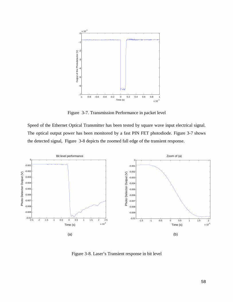
58

-1 -0.8 -0.6 -0.4 -0.2 0 0.2 0.4 0.6 0.8 1 x 10 -4

-7

-6

-5

-4

-3

-2

-1

0 x 10 -3

Time (s)

Out

put o

f the

Pho

tode

tect

or (V

)

Figure 3-7. Transmission Performance in packet level

Speed of the Ethernet Optical Transmitter has been tested by square wave input electrical signal.

The optical output power has been monitored by a fast PIN FET photodiode. Figure 3-7 shows

the detected signal, Figure 3-8 depicts the zoomed fall edge of the transient response.

Figure 3-8. Laser’s Transient response in bit level

-2.5 -2 -1.5 -1 -0.5 0 0.5 1 1.5 2 2.5

x 10-8

-0.01

-0.009

-0.008

-0.007

-0.006

-0.005

-0.004

-0.003

-0.002

-0.001

0

(a)

Time (s)

Pho

to D

etec

tor O

utpu

t (V

)

-1.5 -1 -0.5 0 0.5 1 1.5 2

x 10-9

-0.01

-0.009

-0.008

-0.007

-0.006

-0.005

-0.004

-0.003

-0.002

-0.001

0

Pho

to D

etec

tor O

utpu

t (V

)

Time (s)

(b)

Bit level performance Zoom of (a)

59

We can see from Figure 3-8 that the fall time is 2.5 ns which is fast enough to capture the

ethernet traffic.

• Printed Circuit Board (PCB)

Photograph of the Ethernet Optical Transmitter is shown in Figure 3-9.

Figure 3-9. Overview of the Ethernet Transmitter

This Print Circuit Board (PCB), designed, assembled and tested by Ye Chen and Jean-François

Cliche, consists of 4 layers: Surfacemount parts layer, -5.2 V layer, +5 V layer and Ground

layer, under this case we can get very clean positive and negative power supplies, and avoid

ground loop. The assembly and debug instructions can be found in Appendix I.

3. 3 dB Coupler

Figure 3-10. 3dB Coupler

P1

P2

(P1+P2)/2

(P1+P2)/2

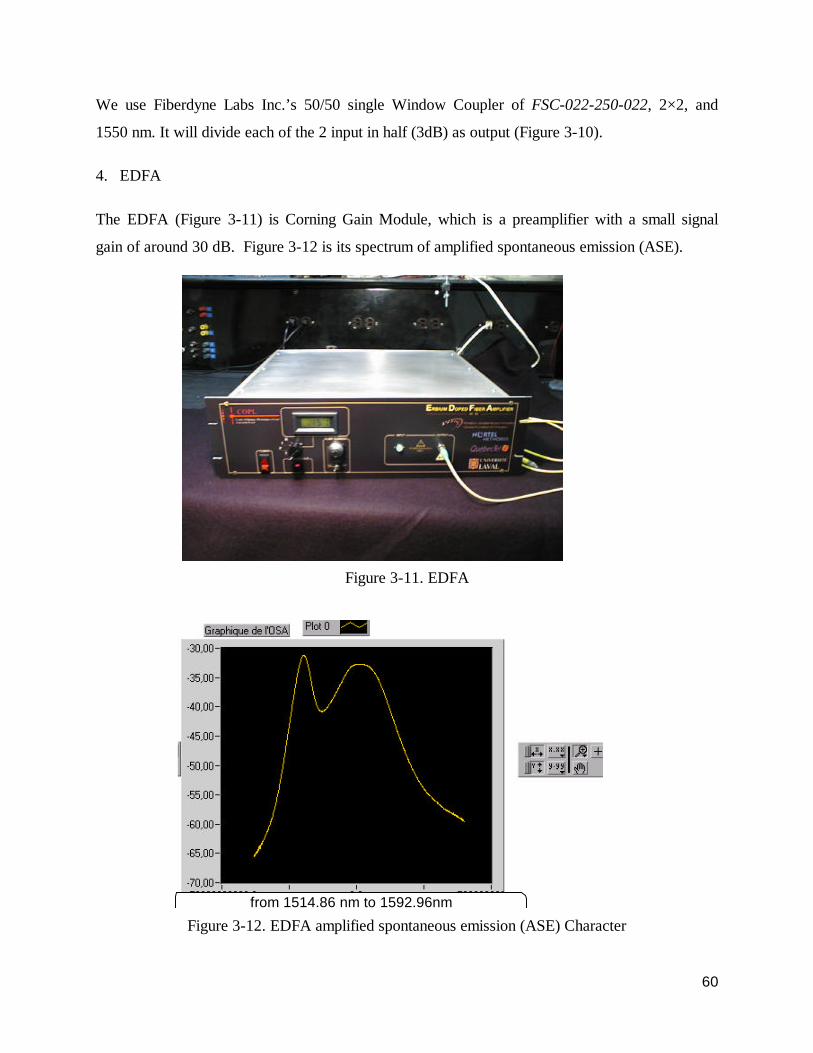
60

We use Fiberdyne Labs Inc.’s 50/50 single Window Coupler of FSC-022-250-022, 2×2, and

1550 nm. It will divide each of the 2 input in half (3dB) as output (Figure 3-10).

4. EDFA

The EDFA (Figure 3-11) is Corning Gain Module, which is a preamplifier with a small signal

gain of around 30 dB. Figure 3-12 is its spectrum of amplified spontaneous emission (ASE).

Figure 3-11. EDFA

Figure 3-12. EDFA amplified spontaneous emission (ASE) Character from 1514.86 nm to 1592.96nm

61

5. Circulator and Bragg Grating

The optical circulator is non-reciprocal device that redirects light from port to port sequentially

in one direction only.

Figure 3-13. Optical Circulator and Bragg Grating

From Figure 3-13, the light first input Port 1, and is then reflected by the Bragg grating at certain

wavelength from Port 2 and redirected to Port 3. So they together serve as a bandpass filter.

6. Photodetector

Figure 3-14. ANTEL ARX-GP amplified ultra high-speed photodetector

We use ANTEL ARX-GP amplified ultra high-speed photodetector system (Figure 3-14) to

receive the CW channel data, which is ideal for high-speed, low level light detection from 300-

1700 nm. It consists of a high-speed non–avalanche type PIN photodiode matched with a DC-

coupled microwave GaAs amplifier to provide state-of-the-art gain-bandwidth. The

Port 1

Port 2

Port 3

62

photodetector and amplifier circuitry are housed in a head with a flat window. Power of the

monitoring channel at the input of the optical bandpass filter is focused on the window of the

photodetector using a 10X microscope objective. Signal output is through a 50 Ω -matched SMA

connector on the detector head and a 1-m length of coaxial cable for connection to any 50 Ω

input impedance equipment. Bias voltages for the photodetector and amplifier are supplied from

a separate rechargeable battery-operated power supply.

7. Data Acquisition Hardwares

The Data acquisition hardware setup is shown in Figure 3-15. The output electrical signal from

the photodetector is fed by a coaxial cable terminated with BNC connector to BNC-2110

Accessory board. The BNC-2110 is connected to the PCI-6110E with a shielded cable. Data is

finally transferred to the computer hard drive.

Figure 3-15. Data Acquisition Scheme

• PCI-6110E Data Acquisition Card

For acquisition of the time variable CW channel output power we use the National Instrument’s

PCI-6110E data acquisition hardware. The 6110 E board is a completely Plug and Play,

( NI PCI-6110E)

63

multifunction analog, digital, and timing I/O board for PCI bus computers. The 6110 E board

features a 12-bit ADC per channel with four simultaneously sampling analog inputs, 16-bit

DACs with voltage outputs, eight lines of TTL-compatible digital I/O, and two 24-bit

counter/timers for timing I/O. The 6110 E board is also easily software-configured and

calibrated.

• BNC-2110 Accessory

Figure 3-16. BNC-2110 Accessory

Figure 3-17. Front Panel of BNC-2110

The BNC-2110 (Figure 3-16, Figure 3-17) is a desktop and DIN rail-mountable BNC adapter we

can connect directly to data acquisition (DAQ) devices. The BNC-2110 includes 15 BNC

connectors and a digital screw terminal with 30 pins.

64

The BNC-2110 has a 68-pin I/O connector that connects to the PCI-60XXE and PCI-61XXE

DAQ devices. The BNC-2110 is ideal for simplifying connections between our measurement

apparatus and our DAQ device in laboratory, test, and production environments.

BNC-2110 Connector Signal Description

Front Panel BNC

Connectors

Signal Description

ACH<0..7> Differential Analog Channels 0~7

DAC0OUT Digital to Analog Converter 0 Output----This pin supplies the voltage output of analog output channel 0.

DAC1OUT Digital to Analog Converter 1 Output----This pin supplies the voltage output of analog output channel 1.

EXTREF External Reference----This is the external reference input for analog output circuitry.

PFI0/TRIG1

Programmable Function

Input 0/Trigger 1----As an input, this is either one of the PFIs or the source for the hardware analog trigger.

CTR0OUT Counter 0 Output----This is the output from the General-Purpose Counter 0 Output.

USER1 User-Defined 1----Connected to USER1 digital screw terminal block. This connector allows you to modify a signal depending on your application

USER2 User-Defined 2----Connected to USER2 digital screw terminal block. This connector allows you to modify a signal depending on your application

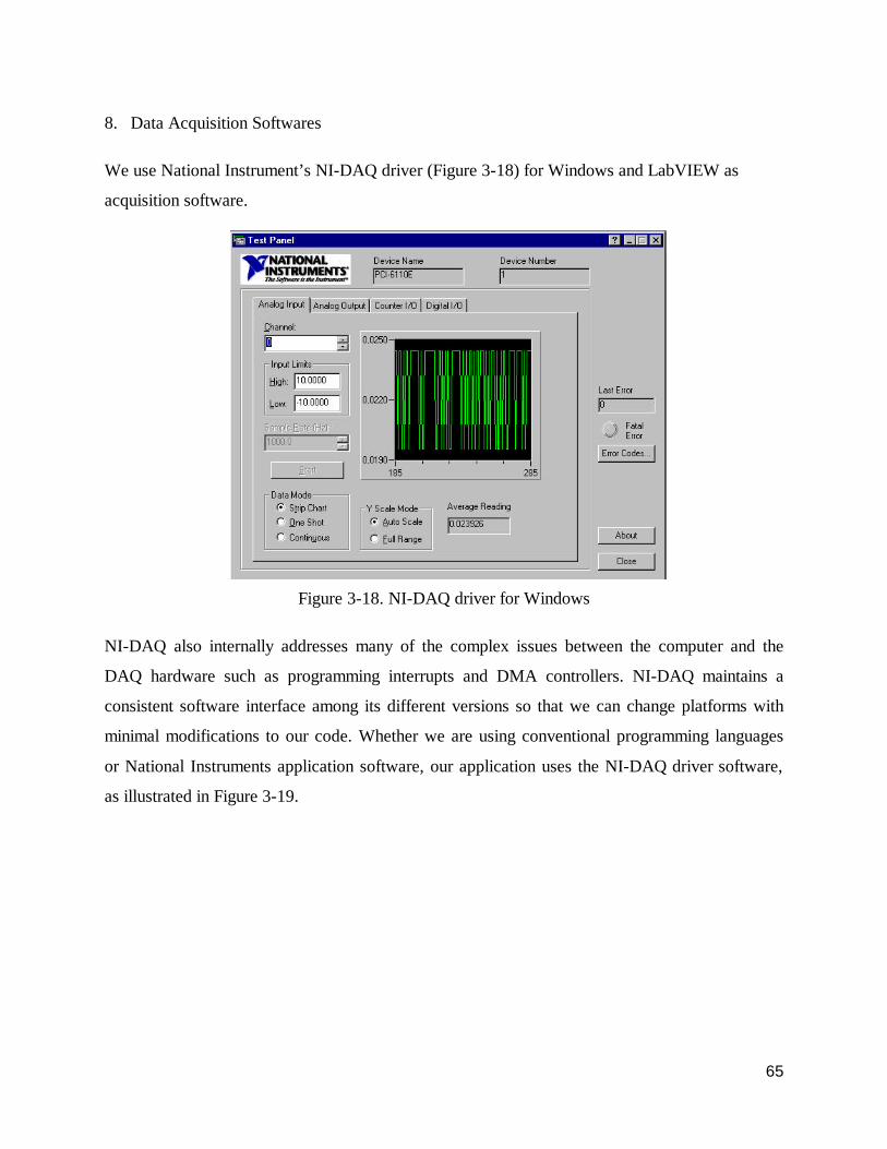
65

8. Data Acquisition Softwares

We use National Instrument’s NI-DAQ driver (Figure 3-18) for Windows and LabVIEW as

acquisition software.

Figure 3-18. NI-DAQ driver for Windows

NI-DAQ also internally addresses many of the complex issues between the computer and the

DAQ hardware such as programming interrupts and DMA controllers. NI-DAQ maintains a

consistent software interface among its different versions so that we can change platforms with

minimal modifications to our code. Whether we are using conventional programming languages

or National Instruments application software, our application uses the NI-DAQ driver software,

as illustrated in Figure 3-19.

66

Figure 3-19. Relationship between the Programming Environment, NI-DAQ and the Hardware

Data is acquired and stored in a binary format using software shown in Figure 3-20, and then it is

converted to ASCII format with a software shown in Figure 3-21. A short Matlab program has

been developed to calculate the Probability Density Function (PDF).

Figure 3-20. LabVIEW DAQ Software Interface

10000.00Scan Rate

10000Buffer Size

5000

# of Scans toWrite at a Time

0Scan Backlog

0

# scans written to file

500000

Max # of scans to write to file

- 1 . 0 0 E + 0

I n t e r c h a n n e l D e l a y ( s e c s )

( -1 :hardw a re defau l t )

H a rdw a re Set t ings

1 . 0 0

high l imit

-1.00

low l imit

0

inpu t l im i t s (no change )

1Device

from your PCStart Date

10:23:01 AMStart Time

STOP

Photo Detector OutputFile Header Text

Output InformationAcquisition Settings

0Channels

ConventionalProgrammingEnvironment

ComponentWorks,LabVIEW,

LabWindows/CVI, orVirtualBench

NI-DAQDriver Software

DAQ orSCXI Hardware

Personal Computeror Workstation

67

The LabVIEW software (Figure 3-20) first acquires the data and stores them in binary format,

then we use another program followed (Figure 3-21) to read and convert them to ASCII format.

Figure 3-21. Read and Convert Program Interface

1000

Block Size toRead at a Time

4 N u m b e r o f C h a n n e l s

in File

1650

0

binary data (I16)

0

# of Scans Readfrom File so far

10 ,00

upper input l imi ts

-10,00

lower input l imi ts

10 ,00

range

bipolar

polar i ty

0 ,50

gain

DC

coup l i ng

di f ferent ia l

i npu t mode

4 , 8 8 2 8 1 E - 3

sca le mul t ip l ie r

0 ,00

sca le o f f se t

0

c h a n n e l0

g r o u p c h a n n e l s e t t i n g s

0 ,80570

0

voltage data

0,00Scan Rate

2,00E-6 I n t e r c h a n n e l D e l a y ( s e c s )

HARDWARE CONFIGURATION FROM FILE

0

Channel L is t in F i le

from your fileStart Date

from your fileStart Time

0

-0

1 0 0 00

0

1

2

3

4

5

6

7

LOGGED DATA

Your header text will appear here.File Header Text

STOP

NEXTBLOCK

mus t be l ess t han t he

amount o f da ta in f i l e

68

Chapter 4 Experimental Results

Introduction

In this chapter we will present measurements of the gain swings in EDFAs handling live

Ethernet data that is self-similar nature.

We will first present results for the time domain and show how long intervals of ON times (when

data is being transferred on the network) and OFF times (when the network is idle) lead to

transients in the EDFA gain. The activity or utilization factor is the percentage of time the

network is not idle. We will examine the response for a single amplifier characterized by the

exponential rise and fall we discussed in chapter 2. Cascades of EDFAs give rise to undershoots

and overshoots in the gain time response (hence gain swings). Finally we will see how clamping

reduces these gain transients significantly.

Next we discuss how the network was manipulated in order to vary the ON and OFF times of the

network, as characterized by the network activity factor. Ethernet data is self-similar, so we

expect that long ON times and long idle times to occur throughout the observation interval,

leading to variation in the gain. We will measure the gain throughout the observation interval

and plot the frequency of occurrence of each gain value, that is a histogram that approximates the

probability density function (PDF) of the gain.

The measurements of the estimated PDF are presented for different network activity factors in a

single EDFA and for a cascade of amplifiers. We will see that extent of gain variation varies

little with activity factor, however the gain variation broadens as we traverse the cascade. Gain

clamping is used to mitigate the gain variation and we examine the time response and gain

variation for single amplifiers as well as cascades.

Finally we compare our results for live Ethernet data with measurements using synthetic data to

approximate a self-similar source, and discuss some challenges we had in implementing the

experiment and the solutions we found.

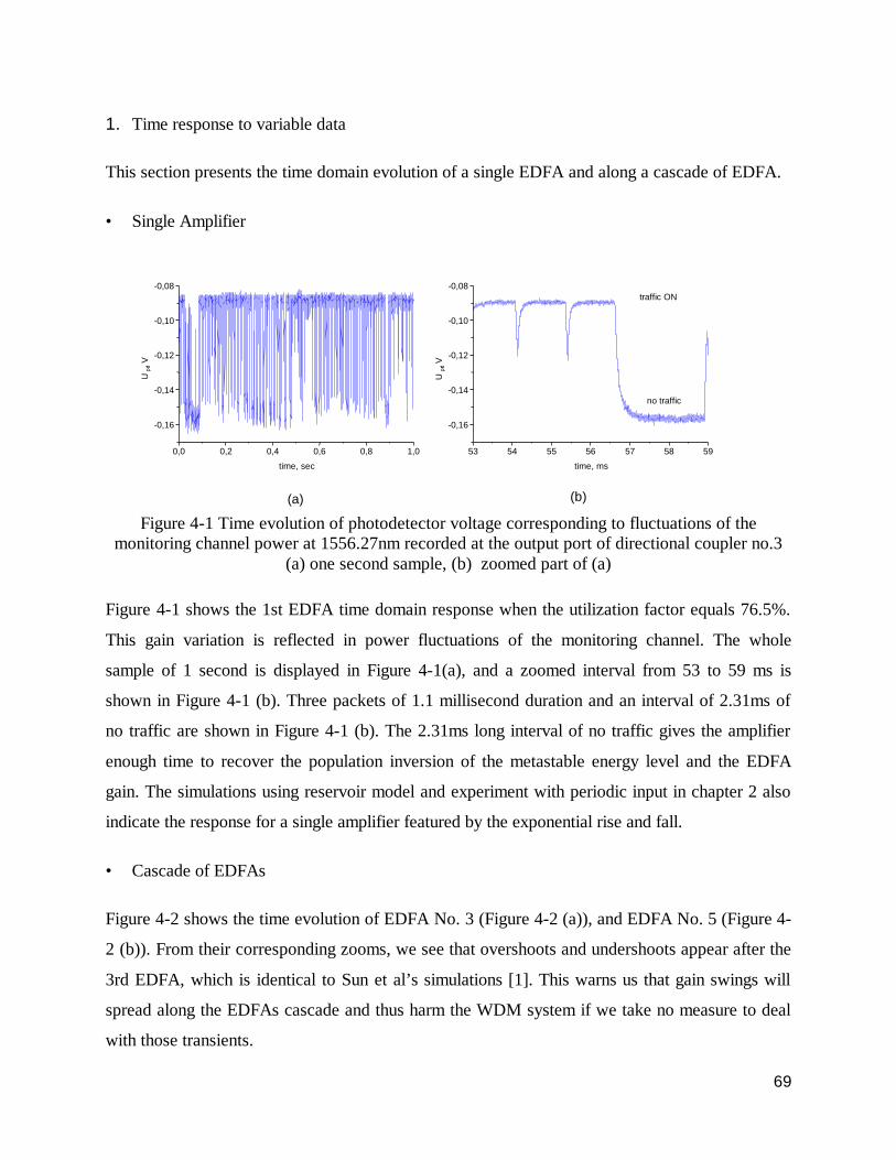
69

1. Time response to variable data

This section presents the time domain evolution of a single EDFA and along a cascade of EDFA.

• Single Amplifier

Figure 4-1 Time evolution of photodetector voltage corresponding to fluctuations of the monitoring channel power at 1556.27nm recorded at the output port of directional coupler no.3

(a) one second sample, (b) zoomed part of (a)

Figure 4-1 shows the 1st EDFA time domain response when the utilization factor equals 76.5%.

This gain variation is reflected in power fluctuations of the monitoring channel. The whole

sample of 1 second is displayed in Figure 4-1(a), and a zoomed interval from 53 to 59 ms is

shown in Figure 4-1 (b). Three packets of 1.1 millisecond duration and an interval of 2.31ms of

no traffic are shown in Figure 4-1 (b). The 2.31ms long interval of no traffic gives the amplifier

enough time to recover the population inversion of the metastable energy level and the EDFA

gain. The simulations using reservoir model and experiment with periodic input in chapter 2 also

indicate the response for a single amplifier featured by the exponential rise and fall.

• Cascade of EDFAs

Figure 4-2 shows the time evolution of EDFA No. 3 (Figure 4-2 (a)), and EDFA No. 5 (Figure 4-

2 (b)). From their corresponding zooms, we see that overshoots and undershoots appear after the

3rd EDFA, which is identical to Sun et al’s simulations [1]. This warns us that gain swings will

spread along the EDFAs cascade and thus harm the WDM system if we take no measure to deal

with those transients.

0,0 0,2 0,4 0,6 0,8 1,0

-0,16

-0,14

-0,12

-0,10

-0,08

U pd ,

V

time, sec

53 54 55 56 57 58 59

-0,16

-0,14

-0,12

-0,10

-0,08

no traffic

traffic ON

U

pd , V

time, ms

(a) (b)

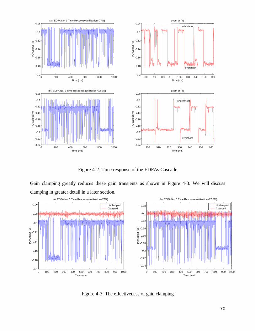
70

Figure 4-2. Time response of the EDFAs Cascade

Gain clamping greatly reduces these gain transients as shown in Figure 4-3. We will discuss

clamping in greater detail in a later section.

Figure 4-3. The effectiveness of gain clamping

0 200 400 600 800 1000 -0.24 -0.22 -0.2

-0.18 -0.16 -0.14 -0.12 -0.1

-0.08

PD

Out

put (

V)

Time (ms)

(b). EDFA No. 5 Time Response (utilization=72.5%)

900 910 920 930 940 950 960 -0.24 -0.22 -0.2

-0.18 -0.16 -0.14 -0.12 -0.1

-0.08 undershoot

overshoot P

D O

utpu

t (V

)

Time (ms)

zoom of (b)

0 200 400 600 800 1000 -0.2

-0.18

-0.16

-0.14

-0.12

-0.1

-0.08

PD

Out

put (

V)

Time (ms)

(a). EDFA No. 3 Time Response (utilization=77%)

80 90 100 110 120 130 140 150 160 -0.2

-0.18

-0.16

-0.14

-0.12

-0.1

-0.08 undershoot

overshoot

zoom of (a)

PD

Out

put (

V)

Time (ms)

0 100 200 300 400 500 600 700 800 900 1000 -0.2

-0.18

-0.16

-0.14

-0.12

-0.1

-0.08

-0.06

Time (ms)

PD

Out

put (

V)

(a). EDFA No. 3 Time Response (utilization=77%) Unclamped Clamped

0 100 200 300 400 500 600 700 800 900 1000 -0.24 -0.22 -0.2

-0.18 -0.16 -0.14 -0.12 -0.1

-0.08

Time (ms)

PD

Out

put (

V)

(b). EDFA No. 5 Time Response (utilization=72.5%) Unclamped Clamped

71

2. Ethernet Data

As follows from the theoretical studies [31, 32, 33], the effect of cross-gain modulation depends

on the statistical features of the packetized traffic. The overall network

utilization][][

][

offon

on

TETETE+

=ρ is used to describe the statistical features of the traffic. Traffic

with different utilization factor has been generated to evaluate the effect of traffic statistics.

We generate variable Ethernet network traffic by:

(i). Playing movie files in Centre d'Optique, Photonique et Laser (COPL)’s Ethernet LAN

environment. According to Figure 4-4, we play a movie with the name of the Red Valley in

MPEG format on the station Saphir while the movie file is located in station Beryl. This can

generate approximately 15% of network utilization. If we play this file simultaneously on

stations Citrine, Prague and Saphir, they can bring the traffic up to 45%~60% load.

Figure 4-4. Traffic Generation

(ii). Copying files among these LAN stations, downloading big files from some websites such as

http://www.oracle.com. This kind of method can generate huge load of traffic, while these

kinds of traffic are not stable and predictable.

Ethernet

Beryl

Vidocq (Server)

Saphir

CenterCOM MR820TR (Hub)

Ethernet Uplink toInternet

Citrine

Prague

Video Source File

72

From [31-34], we know that the self-similar traffic will impact the gain’s PDF (i.e. the frequency

of occurrence of each gain value that is a histogram that approximates the probability density

function of the gain) of EDFAs cascade by the following manner.

• When the first EDFA is unclamped, the gain has a broad PDF that has 2 edges with a middle

mild peak between them. The PDF is constrained in the range between a maximum (reached

when the modulated signal is always OFF) and a minimum (modulated signal always ON).

The edge peaks (ideally Dirac delta function) correspond to the finite probability that the

probe power takes on the steady state maximum and minimum values. For smaller values of

a (higher variability), such edge peaks become higher. The right peak (corresponding to

Signal OFF) will decrease when the network load increases, the left peak (corresponding to

Signal ON) will increase. If network utilization value ρ is different from 0.5 the PDF loses its

symmetry, the double peaks will change their relative position when the utilization factor

varies. The PDF will broaden along the cascade until it saturates.

• When the first EDFA is clamped, the PDF has a bell shape. Clamping has the effect of

significantly narrowing the PDF’s width. In the unclamped case, the PDF of the clamped

case does not change much with variable network load in comparison to unclamped case.

3. Measurements of gain swings

In this section we demonstrate how a cascade of EDFAs respond to live Ethernet traffic with

different activity factors statistically.

• Effect of different activity factors---single EDFA

Figure 4-5 shows the PDF of the output of the 1st EDFA under different utilization factors if the

1st EDFA is not clamped.

We can see that ?=50% is the double peaks’ balance point, the double peaks will be undulating

when network utilization varies. The right peak (corresponding to Signal OFF) decreases with

increasing network load, the left peak (corresponding to Signal ON), on the contrary, increases.

73

Figure 4-5. PDF of the 1st EDFA

The single EDFA’s experimental result agrees with former theoretical study.

• Effect of different activity factors---cascade of EDFAs

Figure 4-6. PDF of the 3rd EDFA

-22 -21 -20 -19 -18 -17 -16 -15 10 -7

10 -6

10 -5

10 -4

10 -3

10 -2

10 -1

10 0 1st EDFA

PD

F

Voltage (dBV)

Utilization=6% Utilization=49% Utilization=77%

-22 -21 -20 -19 -18 -17 -16 -15 -14 10 -7

10 -6

10 -5

10 -4

10 -3

10 -2

10 -1

10 0

Voltage (dBV)

PD

F

the third EDFA

Utilization=23% Utilization=51% Utilization=77%

74

The third EDFA’s output PDF is shown in Figure 4-6, we see they also have two peaks

corresponding to ON/OFF stages. We also see gain swings taking place in this EDFA, so the

PDFs are broader than that of EDFA No. 1. We can find still broader PDFs after EDFA No. 5 in

Figure 4-7 in which we plot both its PDFs and time domain response.

Figure 4-7. Output of the 5th EDFA

The single EDFA’s responses at different positions to different network loads of live Ethernet

traffic are investigated. They are in accordance with [31-34].

From a statistical point of view, when network utilization varies, the monitoring channel is also

changing dramatically, and this indicates the system of WDM will suffer nonnegligible gain

swings, and this kind of harm will accumulate and worsen along the cascade as we will see in

next section.

• Gain swing in cascade

In this section we fix the activity factor ? and focus our attention on how the PDF of the gain is

broadening along the cascade of EDFAs.

• Broadening along the cascade

-21 -20 -19 -18 -17 -16 -15 -14 -13 -12 -1110-7

10-6

10-5

10-4

10-3

10-2

10-1

100

Utilization=4% Utilization=51%Utilization=82%

PD

F

PD Output (dBV)

The 5th EDFA

OvershootsUndershoots

0 1 2 3 4 5 6 7 8-0.24

-0.22

-0.2

-0.18

-0.16

-0.14

-0.12

-0.1

-0.08

Undershoots

Overshoots

Undershoots

Overshoots

(a) (b)

Time (ms)

PD

Out

put (

V)

Overshoots & Undershoots

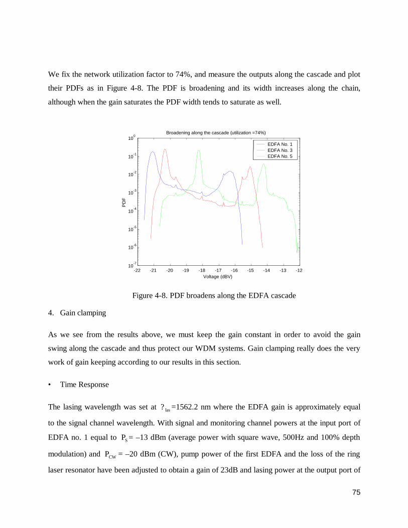
75

We fix the network utilization factor to 74%, and measure the outputs along the cascade and plot

their PDFs as in Figure 4-8. The PDF is broadening and its width increases along the chain,

although when the gain saturates the PDF width tends to saturate as well.

Figure 4-8. PDF broadens along the EDFA cascade

4. Gain clamping

As we see from the results above, we must keep the gain constant in order to avoid the gain

swing along the cascade and thus protect our WDM systems. Gain clamping really does the very

work of gain keeping according to our results in this section.

• Time Response

The lasing wavelength was set at las? =1562.2 nm where the EDFA gain is approximately equal

to the signal channel wavelength. With signal and monitoring channel powers at the input port of

EDFA no. 1 equal to SP = –13 dBm (average power with square wave, 500Hz and 100% depth

modulation) and CWP = –20 dBm (CW), pump power of the first EDFA and the loss of the ring

laser resonator have been adjusted to obtain a gain of 23dB and lasing power at the output port of

-22 -21 -20 -19 -18 -17 -16 -15 -14 -13 -12 10 -7

10 -6

10 -5

10 -4

10 -3

10 -2

10 -1

10 0

Voltage (dBV)

PD

F Broadening along the cascade (utilization =74%)

EDFA No. 1 EDFA No. 3 EDFA No. 5

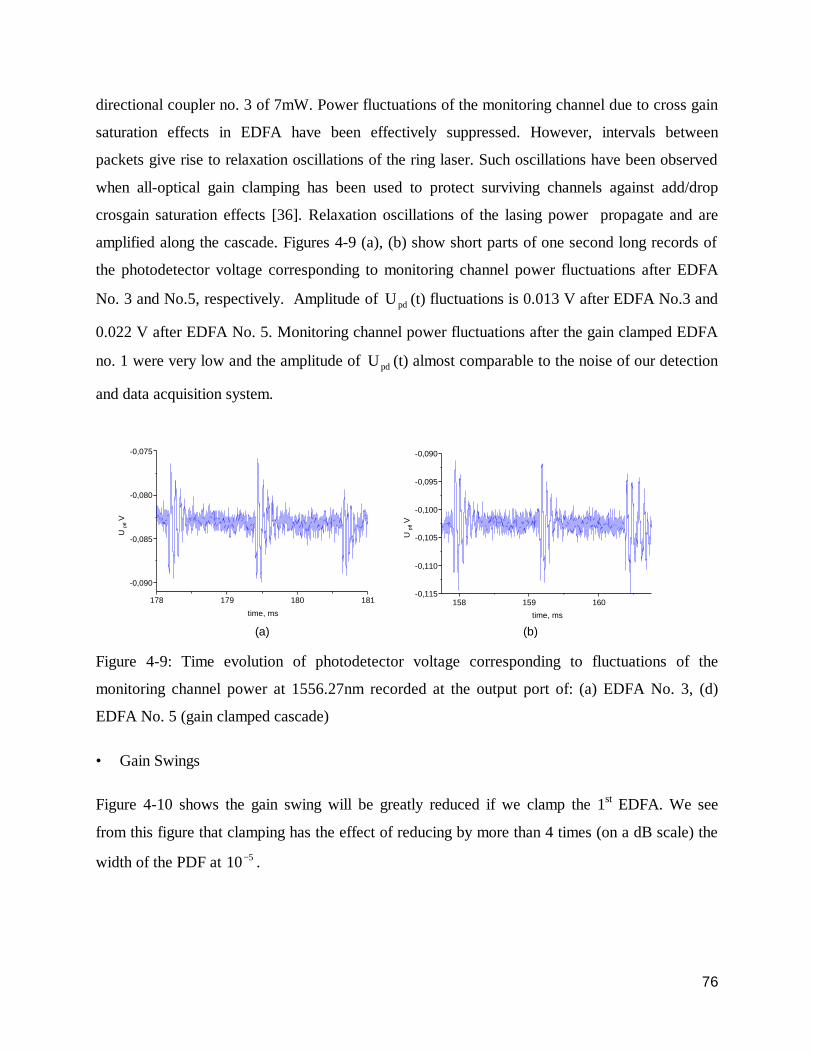
76

directional coupler no. 3 of 7mW. Power fluctuations of the monitoring channel due to cross gain

saturation effects in EDFA have been effectively suppressed. However, intervals between

packets give rise to relaxation oscillations of the ring laser. Such oscillations have been observed

when all-optical gain clamping has been used to protect surviving channels against add/drop

crosgain saturation effects [36]. Relaxation oscillations of the lasing power propagate and are

amplified along the cascade. Figures 4-9 (a), (b) show short parts of one second long records of

the photodetector voltage corresponding to monitoring channel power fluctuations after EDFA

No. 3 and No.5, respectively. Amplitude of pdU (t) fluctuations is 0.013 V after EDFA No.3 and

0.022 V after EDFA No. 5. Monitoring channel power fluctuations after the gain clamped EDFA

no. 1 were very low and the amplitude of pdU (t) almost comparable to the noise of our detection

and data acquisition system.

Figure 4-9: Time evolution of photodetector voltage corresponding to fluctuations of the

monitoring channel power at 1556.27nm recorded at the output port of: (a) EDFA No. 3, (d)

EDFA No. 5 (gain clamped cascade)

• Gain Swings

Figure 4-10 shows the gain swing will be greatly reduced if we clamp the 1st EDFA. We see

from this figure that clamping has the effect of reducing by more than 4 times (on a dB scale) the

width of the PDF at 510 − .

178 179 180 181 -0,090

-0,085

-0,080

-0,075

U pd ,

V

time, ms

158 159 160 -0,115

-0,110

-0,105

-0,100

-0,095

-0,090

U pd ,

V

time, ms (a) (b)

77

Figure 4-10 shows that gain clamping is also valid in reducing the gain swing along the cascade.

Although under the clamping case, the PDF also broadens a little but not so much as the

unclamped case.

Figure 4-10. Clamping also reduces the gain swing in the cascade

Figure 4-11. Output of EDFA 1 under clamped and unclamped cases

Figure 4-11 shows both time evolution and PDF of the first EDFA under clamped and unclamped

case, and we see that the gain swing in single EDFA is reduced. In the clamped case the PDF has a bell

shape. The PDF of the clamped case does not change much with variable network load.

0 0.1 0.2 0.3 0.4 0.5 0.6 0.7 0.8 0.9 1 1 1.5

2 2.5

3 3.5

4 4.5

5 5.5

6

Clamped

Unclamped

Time Evolution of the PD Ouput with Sampling rate of 4 MS/s

Time (s)

Inve

rse

Am

plifi

ed P

D O

utpu

t (V

)

Utilization=16.43% Utilization=62.61%

2 4 6 8 10 12 14 16 10 -7

10 -6

10 -5

10 -4

10 -3

10 -2

10 -1

Voltage (dBV)

PD

F

Clamped

Unclamped

PDF of the PD Output Utilization=16.43% Utilization=62.61%

-23 -22 -21 -20 -19 -18 -17 -16 -15 -14 -13 -12 10 -6

10 -4

10 -2

10 0

Voltage (dBV)

PD

F Unclamped----Utilization 74%

1st EDFA 3rd EDFA 5th EDFA

-23 -22 -21 -20 -19 -18 -17 -16 -15 -14 -13 -12 10 -6

10 -4

10 -2

10 0

Voltage (dBV)

PD

F

Clamped 3rd EDFA 5th EDFA

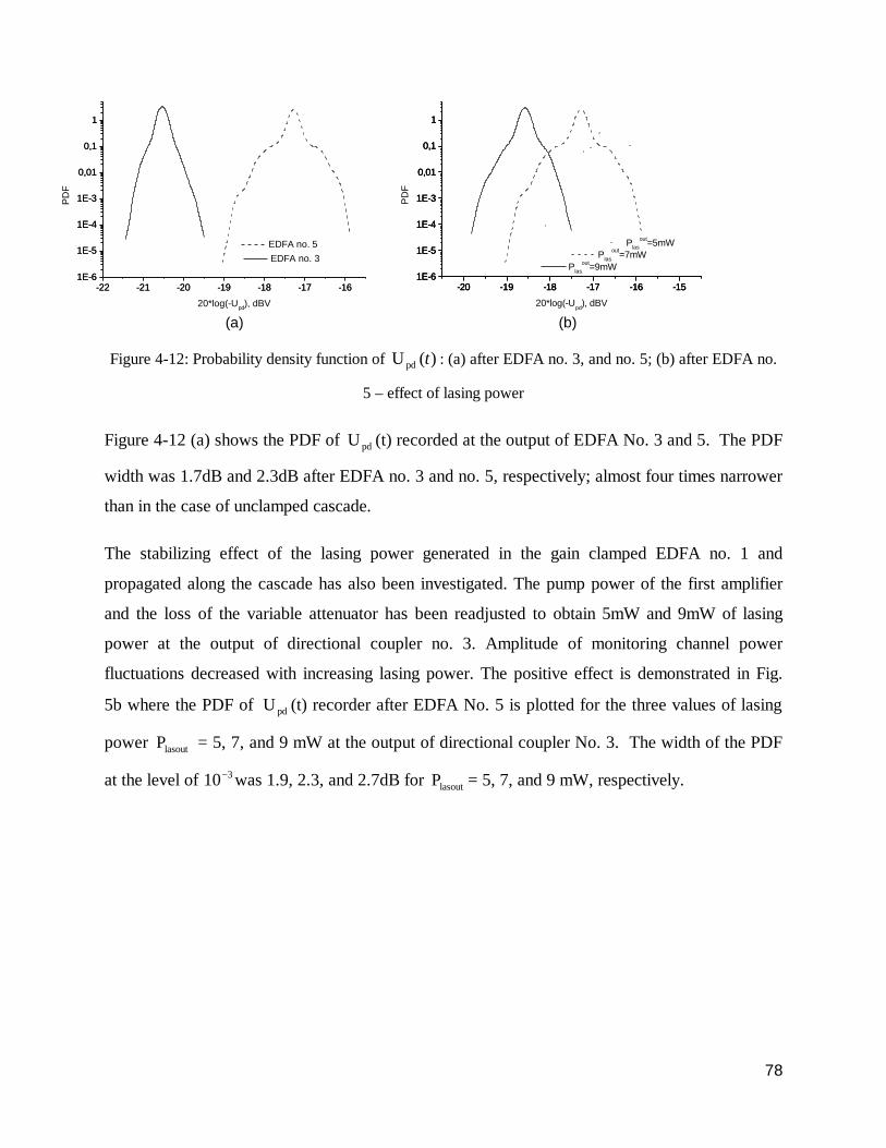
78

Figure 4-12: Probability density function of )(U pd t : (a) after EDFA no. 3, and no. 5; (b) after EDFA no.

5 – effect of lasing power

Figure 4-12 (a) shows the PDF of pdU (t) recorded at the output of EDFA No. 3 and 5. The PDF

width was 1.7dB and 2.3dB after EDFA no. 3 and no. 5, respectively; almost four times narrower

than in the case of unclamped cascade.

The stabilizing effect of the lasing power generated in the gain clamped EDFA no. 1 and

propagated along the cascade has also been investigated. The pump power of the first amplifier

and the loss of the variable attenuator has been readjusted to obtain 5mW and 9mW of lasing

power at the output of directional coupler no. 3. Amplitude of monitoring channel power

fluctuations decreased with increasing lasing power. The positive effect is demonstrated in Fig.

5b where the PDF of pdU (t) recorder after EDFA No. 5 is plotted for the three values of lasing

power lasoutP = 5, 7, and 9 mW at the output of directional coupler No. 3. The width of the PDF

at the level of 310 − was 1.9, 2.3, and 2.7dB for lasoutP = 5, 7, and 9 mW, respectively.

-22 -21 -20 -19 -18 -17 -161E-6

1E-5

1E-4

1E-3

0,01

0,1

1

EDFA no. 3

PD

F

20*log(-Upd), dBV

-22 -21 -20 -19 -18 -17 -161E-6

1E-5

1E-4

1E-3

0,01

0,1

1

EDFA no. 5

-20 -19 -18 -17 -16 -151E-6

1E-5

1E-4

1E-3

0,01

0,1

1

Plasout=9mW

PD

F

20*log(-Upd), dBV

-20 -19 -18 -17 -16 -151E-6

1E-5

1E-4

1E-3

0,01

0,1

1

Plasout=7mW

-20 -19 -18 -17 -16 -151E-6

1E-5

1E-4

1E-3

0,01

0,1

1

Plasout=5mW

(a) (b)

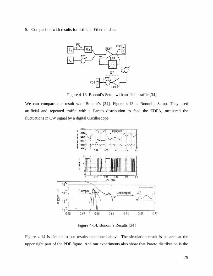
79

5. Comparison with results for artificial Ethernet data

Figure 4-13. Bononi’s Setup with artificial traffic [34]

We can compare our result with Bononi’s [34]. Figure 4-13 is Bononi’s Setup. They used

artificial and repeated traffic with a Pareto distribution to feed the EDFA, measured the

fluctuations in CW signal by a digital Oscilloscope.

Figure 4-14. Bononi’s Results [34]

Figure 4-14 is similar to our results mentioned above. The simulation result is squared at the

upper right part of the PDF figure. And our experiments also show that Pareto distribution is the

80

good choice to model self-similar network traffic, because by simulation and artificial traffic

experimental results mentioned in earlier sections, they predicted the PDF shape of the EDFA’s

response by supposing that the traffic has a Pareto distribution.

6. Experimental implementation

In order to decrease the digitization error due to weak CW signal fluctuations after EDFA No. 1,

we can put an inverse electronic amplifier after the PD and before the data acquisition card, or

get the value without inverse electronic amplifier for every 10~20 points’ mean, or even use the

data acquisition card’s maximum sampling rate of 5 MS/s.

If we do not have any band-pass filter, we can also use Figure 2-12’s quick setup.

81

Chapter 5. Conclusions

1. What was achieved

EDFA gain dynamics in WDM systems was studied in this work. For the first time we have

measured the response of EDFAs fed by live Ethernet data at 10 Mb/s and verified previous

theoretical results where packetized data is modeled as having self-similar characteristics.

We built an Ethernet transmitter, captured the network traffic from the LAN Ethernet by the

transmitter and thus converted the traffic from electrical level to optical signal. 5 EDFAs were

finely adjusted and linked together. Data acquisition system is composed of the PCI-6110E data

acquisition card and LabVIEW program.

Analysis of the data acquired by the data acquisition system showed, in the unclamped case,

substantial gain variation after 5 EDFA in a cascade caused by gain fluctuation in burst-mode

packet switched network. The implementation of gain clamping is extremely effective to combat

the gain variation.

Our experimental results demonstrate that substantial swings in EDFA output power can be

induced by crossgain saturation when packetized bursty traffic is transmitted through a cascade

of fiber amplifiers. Amplitude of these swings grows along the cascade in the same way as

surviving channel fluctuations when channels are dropped/added in a WDM circuit-switching

scenario. Although our experimental setup allowed us to transmit the packetized traffic over one

channel, only numerical simulations [33] predict that even in 8 channel WDM system with

bursty traffic the probability of long empty slots is rather high and can give rise to large

fluctuations of EDFA gain.

The stabilizing effect of clamping the gain of the first amplifier in the cascade by a ring laser

configuration and propagating the lasing power through the cascade has been confirmed. The

width of the PDF of the monitoring channel power at the output of the cascade of five amplifiers

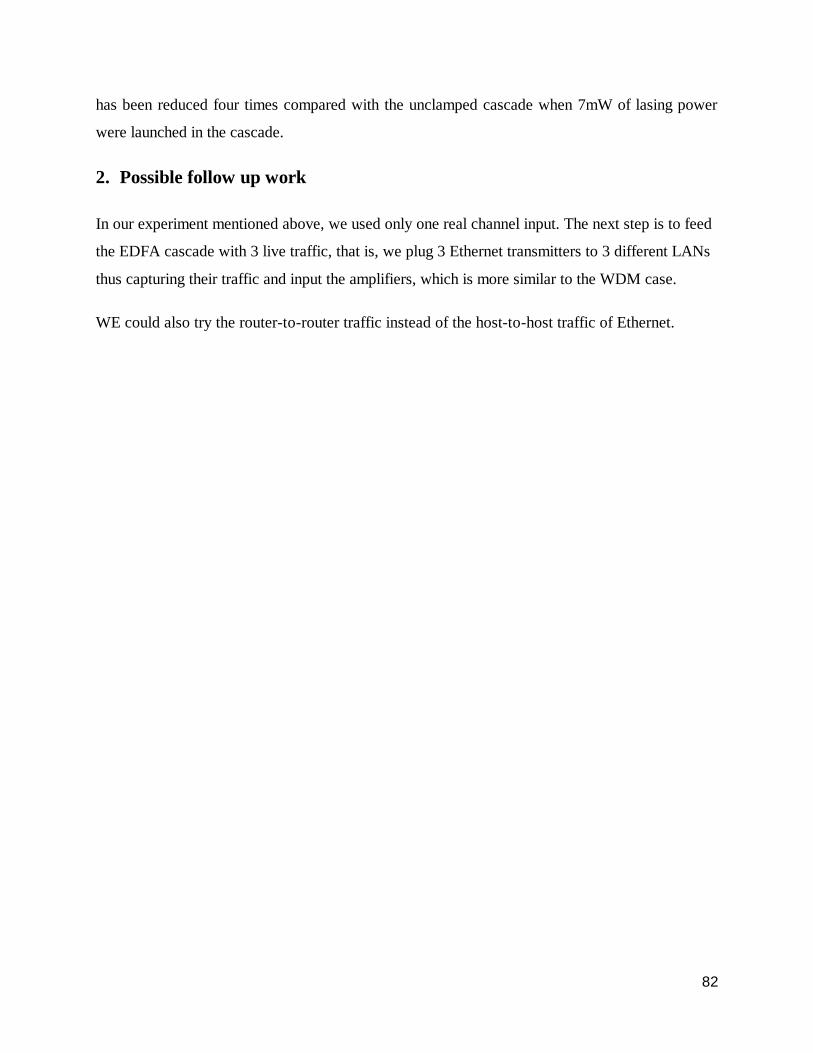
82

has been reduced four times compared with the unclamped cascade when 7mW of lasing power

were launched in the cascade.

2. Possible follow up work

In our experiment mentioned above, we used only one real channel input. The next step is to feed

the EDFA cascade with 3 live traffic, that is, we plug 3 Ethernet transmitters to 3 different LANs

thus capturing their traffic and input the amplifiers, which is more similar to the WDM case.

WE could also try the router-to-router traffic instead of the host-to-host traffic of Ethernet.

83

References:

[1] Y. Sun, A. K. Srivastava, J.L. Zyskind, J.W. Sulhoff, C.Wolf, and R.W. Tkach, Fast power

transients in WDM optical networks with cascaded EDFA's. Electron. Lett., vol. 33.,

pp. 313-314, 1997.

[2] J.L. Zyskind, Y. Sun, A.K. Srivastava, J.W. Sulhoff, A.J. Lucero, C. Wolf, and R.W. Tkach,

Fast power transients in optically amplified multiwavelength optical networks. Proc.

OFC '96 Techn. Digest, San Jose, CA, Paper TD 31-1.

[3] M. Karasek, Fast power transients in concatenated Pr3+-doped fluoride fiber amplifiers.

J. Lightwave Technol., vol. 16, pp.358-363, 1998.

[4] A.K. Srivastava, Y.Sun, J.L. Zyskind, and J.W. Sulhoff, EDFA transient response to

channel loss in WDM transmission system. IEEE Photon. Technol. Lett., vol. 9, pp.386-

388, 1997.

[5] M. Karasek, and J.C. van der Plaats, Analysis of dynamic pump-loss controlled gain-

locking system for erbium-doped fiber amplifiers, IEEE Photon. Technol. Lett., vol. 10,

pp.1171-1173, 1998.

[6] A.K. Srivastava, J.L. Zyskind, Y. Sun, J. Ellson, G. Newsome, R.W. Tkach, A.R. Chraplyvy,

J.W. Sulhoff, T.A. Strasser, C. Wolf, and J.R. Pedrazzani,Fast-link control protection of

surviving channels in multiwavelength optical networks. IEEE Photon. Technol. Lett.,

vol. 9, pp.1667-1669, 1997.

[7] H. Dai, J.Y Pan, and Ch. Lin, All-optical gain control of in-line erbium-doped fiber

amplifiers for hybrid analog/digital WDM systems. IEEE Photon. Technol. Lett., vol. 9,

pp.737-739, 1997.

[8] D.H. Richards, J.L. Jackel, and M.A. Ali, Multichannel EDFA chain control: A

comparison of two all-optical approaches. IEEE Photon. Technol. Lett., vol. 10, pp.156--

158, 1998.

84

[9] J. Beran, R. Sherman, M.S. Taqqu, and W. Wilinger, Long-range dependence in variable-

bit-rate video traffic. IEEE Trans. Commun., vol. 43, pp.1566-1579, 1995.

[10] W. Wilinger, M.S. Taqqu, R. Sherman, and D.V. Wilson, Self-similarity through high-

variability: Statistical analysis of Ethernet LAN traffic at the source level. IEEE/ACM

Trans. Networking, vol. 5, pp.71-86, 1997.

[11] M.E. Crovella, and A. Bestavros, Self-similarity in World Wide Web traffic: Evidence

and possible causes, IEEE/ACM Tran. Networking, vol. 5, pp.835-846, 1997.

[12] A. Bononi, L. Tancevski, and L.A. Rusch, Large power swings in doped-fiber amplifiers

with highly variable data, IEEE Photon. Technol. Lett., vol. 10, pp.131-133, 1998.

[13] L. Tancevski, A. Bononi, and L.A. Rusch, Output power and SNR swings in cascades of

EDFAs for circuit- and packet-switched optical networks. J. Ligthwave Technol., vol.

17, pp.733-742, 1999.

[14] A. Bononi, L. Poti, and A. Azzini, Measurement of power spread histograms in chains

of EDFAs fed by multimedia burst-mode packet traffic. Proc. European Conf. Opt.

Commun. 1999, Nice, pp.II-104-105.

[15] Timothy Parker (1996), Teach You TCP/IP in 14 Days. Sams.

[16] Laura Chappell (1998), Introduction to Cisco Router Configuration. Cisco Press.

[17] The Institution of Electrical and Electronic Engineers, Carrier sense multiple access with

collision detection (CSMA/CD) access method and physical layer specifications.

Technical report, The Institution of Electrical and Electronic Engineers, 1985. American

National Standards Institute ANSI/IEEE Std. 802.3-1985.

[18] Xerox Corp. Digital Corp., Intel Corp. The Ethernet: A local area network data link

layer and physical layer specifications, version 2.0. Technical report, Digital Corp., Intel

Corp., Xerox Corp., February 1982.

[17] Alcatel, Optical Networks Tutorial. Webforums, 1999.

85

[18] Georgios Ellinas, Presentation slide for MULTIWAVELENGTH OPTICAL

NETWORKING, Columbia University, 1999.

[19] Mike Sharrif, Packet over SONET for IP Transport. Cisco’s Networkers ’98 Conference

[20] T. HU, IP over DWDM Technology. P&T Business 12, 1999.

[21] W. E. Leland, M. S. Taqqu, W. Willinger, D. V. Wilson, On the self-Similar Nature of

Ethernet Traffic, ACM SIGComm ’93, San Francisco, September 1993.

[22] Ross Alexander, Monitoring, Analysis and Simulation of Packet Switched Network

Traffic, Master thesis of the University of Auckland, 1995.

[23] Desurvire, E. (1994). Erbium-doped fiber amplifiers: principles and applications. New

York, Wiley.

[24] P. E. Green Jr., Fiber Optic Networks, Prentice Hall, 1993.

[25] B. E. A. Saleh and M. C. Teich, Fundamentals of Photonics, John Wiley & Sons, New

York, 1991.

[26] R. Olshansky, Noise figure for erbium-doped optical fiber amplifiers, Electronics

Letters, vol. 24, no. 22, pp. 1363, 1988.

[27] Y. Sun, J. L. Zyskind, and A. K. Srivastava, Average inversion level, modeling, and

physics of erbium-doped fiber amplifiers, IEEE Journal on Selected Topics in Quantum

Electronics, vol. 3, no. 4, pp. 991-1007, August, 1997.

[28] Alberto Bononi and Leslie A. Rusch, Doped-Fiber Amplifier Dynamics: A System

Perspective, IEEE Journal of Lightwave Technology vol. 16, no. 5, pp. 945-956, May

1998.

[29] A. K. Srivastava, Y. Sun, J. L. Zyskind, and J. W. Sulhoff, EDFA transient response to

channel loss in WDM transmission system, IEEE Photonics Technology Letters, vol. 9,

no. 3, pp. 386-388, March 1997.

86

[30] A. Bononi, L. Barbieri, Design of Gain-Clamped Doped-Fiber Amplifiers for Optimal

Dynamic Performance, Journal of Lightware Technology, Vol. 17, No.7, July 1999.

[31] A. Bononi, L. Tancevski, and L.A. Rusch, Large power swings in doped-fiber amplifiers

with highly variable data, IEEE Photon. Technol. Lett., vol. 10, pp.131-133, 1998.

[32] L. Tancevski, A. Bononi, and L.A. Rusch, Output power and SNR swings in cascades of

EDFAs for circuit- and packet-switched optical networks, J. Ligthwave Technol., vol. 17,

pp.733-742, 1999.

[33] M. Karasek, A. Bononi, L.A. Rusch, and M. Menif, Gain stabilization in gain clamped

EDFA cascades fed by burst-mode packet traffic, J. Ligthwave Technol., vol. 18, pp308-

313, 2000.

[34] A. Bononi, L. Poti, and A. Azzini, Measurement of power spread histograms in chains of

EDFAs fed by multimedia burst-mode packet traffic. Proc. European Conf. Opt. Commun.

1999, Nice, pp.II-104-105.

[35] Cisco Systems, Cisco’s Networkers’ ’98 presentation CD, 1998.

[36] G. Luo, J.L. Zyskind, Y. Sun, A.K. Srivastava, J.W. Sulhoff, C. Wolf, and M.A. Ali,

Performance degradation of all-optical gain-clamped EDFA’s due to relaxation-oscillations

and spectral-hole burning in amplified WDM networks, IEEE Photon. Technol. Lett., vol.

9, pp.1346-1348, 1997.

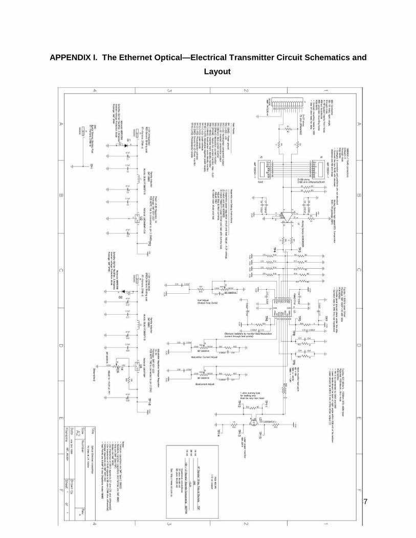
87

APPENDIX I. The Ethernet Optical— Electrical Transmitter Circuit Schematics and

Layout

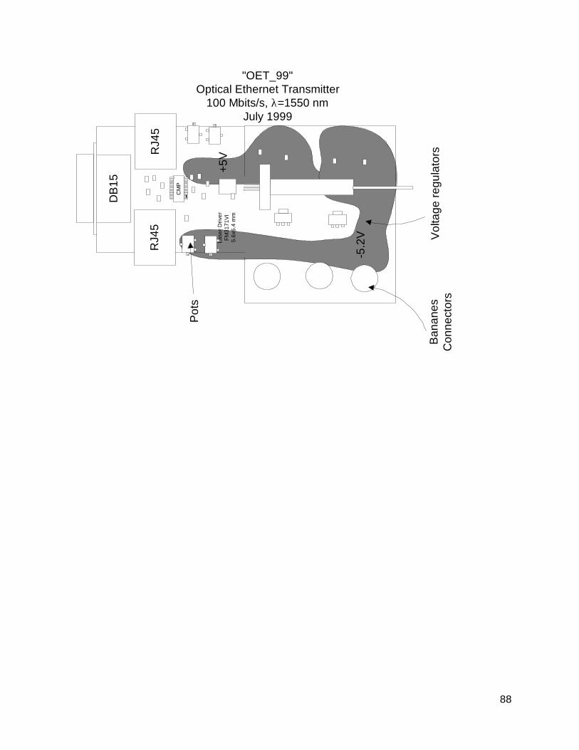
88

Lase

r Driv

erFM

3171

VI

5.6x

6.4

mm

RJ4

5

DB

15

CM

P-

RJ4

5

-5.2

V

+5V

"OET_99"Optical Ethernet Transmitter

100 Mbits/s, λ=1550 nmJuly 1999

Pot

s

Ban

anes

Con

nect

ors

Vol

tage

regu

lato

rs

89

Appendix II AUI on 10 Base-T Ethernet Hub

• A hub is a common connection point for devices in a network. Hubs are commonly used to

connect segments of a LAN. A hub contains multiple ports. When a packet arrives at one

port, it is copied to the other ports so that all segments of the LAN can see all packets. A

passive hub serves simply as a conduit for the data, enabling it to go from one device (or

segment) to another. So-called intelligent hubs include additional features that enable an

administrator to monitor the traffic passing through the hub and to configure each port in the

hub. Intelligent hubs are also called manageable hubs. A third type of hub, called a

switching hub, actually reads the destination address of each packet and then forwards the

packet to the correct port.

• AUI, short for Attachment Unit Interface, is the portion of the Ethernet standard that specifies

how a cable is to be connected to an Ethernet card. AUI specifies a coaxial cable connected

to a transceiver that plugs into a 15-pin socket on the network interface card (NIC). We tap

off the Ethernet traffic from this DB15 port and drive the laser, the pin assignment is as

followed:

1. not used

2. "C+" : Collision + (output from MAU)

A signal to indicate that multiple stations are contending for access to the transmission medium.

3. "T+" : Transmit + (input to MAU)

This line is intended to operate into terminated transmission lines.

4. not used

5. "R+" : Receive + (output from MAU)

90

a data input sourced by the MAU.

6. GND : GROUND

7. not used

8. not used

9. "C-" : Collision - (output from MAU)

10. "T-" : Transmit - (input to MAU)

11. not used

12. "R-" : Receive - (output from MAU)

13. +12VF : +12Vdc Power (fused)

fused +12Vdc sourced by the DTE

14. not used

15. not used

• Category 5 cable pinout and connection