Effect of Driver Behavior on Spatiotemporal Congested Traffic

Patterns at Highway Bottlenecks in the Framework of Three-Phase

Traffic Theory

Boris S. Kerner*

Daimler AG, GR/PTF, HPC: G021, 71059 Sindelfingen, Germany

Abstract

We present results of numerical simulations of the effect of driver behavior on spatiotemporal congested traffic patterns that

result from traffic breakdown at an on-ramp bottleneck. The simulations are made with the Kerner-Klenov stochastic traffic flow

model in the framework of three-phase traffic theory. Different diagrams of congested patterns at the bottleneck associated with

different driver behavioral characteristics are found and compared each other. An adaptive cruise control (ACC) in the

framework of three-phase traffic theory introduced by the author (called a “driver alike ACC” (DA-ACC)) is discussed. The

effect of DA-ACC-vehicles on traffic flow, in which without the DA-ACC-vehicles traffic congestion occurs at the bottleneck, is

numerically studied. We show that DA-ACC-vehicles improve traffic flow considerably without any reduction in driving

comfort. It is found that there is a critical percentage of DA-ACC-vehicles in traffic flow: If the percentage of the DA-ACC-

vehicle exceeds the critical one no traffic breakdown occurs at the bottleneck. A criticism of a recent “criticism of three-phase

traffic theory” is presented.

Keywords: Traffic congestion; Three-phase traffic theory; Highway bottleneck; Adaptive cruise control (ACC) based on three-phase theory

1. Introduction

The understanding of traffic congestion is the key for development of many other fields of transportation science

and engineering. For this reason, a huge number of publications, reviews, and books are devoted to empirical studies

of traffic congestion and associated traffic flow theories (see references in Haight, 1963; Drew, 1968; Prigogine and

Herman, 1971; Whitham, 1974; Wiedemann, 1974; Cremer, 1979; Newell, 1982; Papageorgiou, 1983; Leutzbach,

1988; May, 1990; Daganzo, 1997; Brackstone and McDonald, 1998; Highway Capacity Manual, 2000; Chowdhury

et al., 2000; Gartner et al. (eds), 2001; Helbing, 2001; Gazis, 2002; Nagatani, 2002; Nagel et al., 2003; Mahnke et

al., 2005; Rakha et al., 2009). In empirical observations, traffic breakdown in free flow occurs mostly at bottlenecks

associated with, e.g., on- and off-ramps. In congested traffic, moving jams are observed. A moving jam is a

localized structure of great vehicle density, spatially limited by two jam fronts; the jam propagates upstream; within

the jam vehicle speed is very low. Theoretical studies of traffic congestion at bottlenecks have been made mostly

either in the framework of the Lighthill-Whitham-Richards (LWR) kinematic (shock) wave traffic flow theory or in

the framework of the General Motors (GM) approach by Herman, Gazis, Montroll, Potts, and Rothery.

Although there are many important achievements in the understanding of traffic congestion made in these and

many other works, however, these approaches cannot explain empirical features of traffic breakdown at highway

bottlenecks as found in real measured traffic data. A detailed criticism of the description of traffic breakdown and

resulting congested traffic patterns within the frameworks of the LWR- and GM-approaches as well as other traffic

flow theories reviewed in (May, 1990; Brackstone and McDonald, 1998; Chowdhury et al., 2000; Gartner et al.

(eds), 2001; Helbing, 2001; Gazis, 2002; Nagatani, 2002; Nagel et al., 2003; Mahnke et al., 2005; Rakha et al.,

2009) has been made in (Kerner, 2009). In this article, we have to limit a consideration of our critical responses only

on “criticism of three-phase traffic theory” published in “Transportation Science” and “Transportation Research B”

* Boris S. Kerner. Tel.: + 49-7031-4389566.

E-mail address: boris.kerner@daimler.com.

Boris S. Kerner

2

(Schönhof and Helbing, 2007, 2009). Readers can find all other our criticisms on earlier traffic flow theories and

models in Chapter 10 of the book (Kerner, 2009).

To describe traffic breakdown in accordance with real measured data, the author introduced three-phase traffic

theory reviewed in (Kerner, 2004a, 2009). In this theory, there are (i) the free flow, (ii) synchronized flow, and (iii)

wide moving jam traffic phases. The synchronized flow and wide moving jam phases associated with congested

traffic are defined via the empirical definitions [S] and [J], respectively. A wide moving jam is a moving traffic jam,

i.e., a localized structure of great vehicle density and low speed, spatially limited by two jam fronts, which exhibit

the characteristic jam feature [J] to propagate through bottlenecks while maintaining the mean velocity of the

downstream jam front. Synchronized flow [S] is defined as congested traffic that does not exhibit the jam feature

[J]; in particular, the downstream front of synchronized flow is often fixed at the bottleneck.

The fundamental hypothesis of three-phase traffic theory is that steady states of synchronized flow cover a 2D-

region (S) in the flow-density plane and there is a speed gap between this region and free flow states (F) at each

given density (Fig. 1 (a)). This means also that within the 2D-region each driver tends to adapt its speed to the

preceding vehicle (“speed adaptation”) without caring what a precise space (time) gap is as long as the gap is safe

(Fig. 1 (b)): There is no relationship between the flow rate and density (no fundamental diagram) even for steady

states of synchronized flow. The upper boundary of the 2D-region in Fig. 1 (b) is associated with a so-called

synchronization space gap denoted by G that determines a synchronization time headway; the lower boundary of the

2D-region in Fig. 1 (b) is associated with a safe space gap denoted by safeg that determines a safe time headway.

The first microscopic traffic flow model in which many hypotheses of three-phase traffic theory have been

incorporated is the Kerner-Klenov stochastic three-phase traffic flow model (Sect. 16.3 of Kerner, 2004a). The 2D-

region of steady states of synchronized flow in this model is shown in Fig. 1 (c, d). This model can show traffic

breakdown at a bottleneck and resulting congested patterns as found in empirical data (Kerner, 2004a, 2009). For

this reason, we will use the model for all simulations presented in this article. Author’s three-phase traffic theory is

the theoretical basis for many new traffic flow models and control methods developed recently (see e.g., Davis,

2004, 2006, 2010; Jiang, et al., 2004; Lee et al., 2004; Jia et al., 2009; Gao et al., 2007, 2009).

In the Kerner-Klenov model, a variety of driver behavioral characteristics have been used, which influence

considerably on spatiotemporal congested traffic patterns occurring at a bottleneck (Kerner, 2004a, 2009). However,

in this article we limit a consideration of the influence on the patterns of two driver behaviors only:

(i) the speed adaptation within 2D-region of synchronized flow states of three-phase traffic theory (Kerner,

2004a) and

(ii) the well-known over-deceleration effect of the GM model class associated with a delay in driver

deceleration that is caused by a driver reaction time (Herman, et al., 1958; Gazis et al., 1961).

To demonstrate the importance of this driver behavioral analysis for transportation engineering, we show that if

some of the vehicles in traffic flow move in accordance with an adaptive cruise control (ACC) in the framework of

three-phase traffic theory introduced in (Kerner, 2004b) whose main feature is the speed adaptation within 2D-

region of synchronized flow states (Fig. 1 (b)), then both traffic breakdown and moving jam emergence can be

prevented without any reduction in comfortable driving.

Before we present these novel results, in section “Background” we repeat the Kerner-Klenov model used for all

simulations, basic theoretical features of traffic breakdown and resulting congested patterns at a on-ramp bottleneck

as well as those driver behavioral assumption of the model that are required for the paper understanding.

Boris S. Kerner

3

Fig. 1. Fundamental hypothesis of three-phase traffic theory (Kerner, 2004a): (a, b) Qualitative representation of the hypothesis in the flow-

density (a) and speed-space gap planes (in (b) only a part of 2D synchronized flow states of (a) is shown). (b, c) Steady states of the Kerner-

Klenov stochastic three-phase traffic flow model used in simulations.

2. Background

2.1. Two Classes of Homogeneous Synchronized Flow (HSF) in Three-Phase Traffic Theory

For the understanding of the paper results, firstly we should remember some general features of 2D steady states

of synchronized flow associated with the fundamental hypothesis of three-phase traffic theory (dashed region in

Figs. 1 and 2). Steady states of synchronized flow are homogeneous in space and time. Therefore, synchronized

flow associated with these states can be called “homogeneous synchronized flow” (HSF). Thus in three-phase traffic

theory, at each vehicle density and speed at which synchronized flows exists (2D dashed regions in Fig. 2), a

synchronized flow can be an HSF.

In three-phase traffic theory, an HSF exhibits qualitatively different features depending of whether the HSF is

associated with a state below or above the line J in the flow-density plane (line J in Fig. 2). Recall that the line J

represents the steadily propagation of the downstream front of a wide moving jam in the flow-density plane, i.e., the

slope of the line J is equal to the mean velocity gv of this jam front:

)(1v)a(

jam,delmaxg τρ−= ,

Boris S. Kerner

4

where maxρ is the jam density, )a(

jam,delτ is the mean driver time delays in acceleration at the downstream jam front.

The left and right coordinates of the line J are associated with the maximum jam outflow outq and jam density maxρ ,

respectively.

The feature of HSF is as follows (Kerner, 1998): The line J divides all HSF into two different HSF classes with

respect to wide moving jam formation:

(i) stable HSF,

(ii) metastable HSF.

Stable HSF are associated with states below the line J, whereas metastable HSF are associated with states on and

above the line J (Fig. 4). In a stable HSF, no wide moving jams can emerge and persist independent of whether there

are great fluctuations of time headways, speed, density, and/or flow rate in the HSF or not.

In contrast with the stable HSF, in a metastable HSF a wide moving jam(s) emerges only if speed (space gap)

fluctuations appear that are greater than some critical ones. Otherwise, no wide moving jams emerge.

The general feature of metastable HSFs is as follows (Kerner, 2004a): At the same vehicle speed, the closer time

headway to a safety time headway, the greater the probability of wide moving jam emergence within a metastable

HSF during the same time interval.

Fig. 2. Homogeneous synchronized flow (HSF) of three-phase traffic theory (Kerner, 1998). Free flow states (F) ands 2D-dashed region of

synchronized flow states are taken from Fig. 1 (a).

2.2. Discrete Version of Stochastic Three-Phase Traffic Flow Model

For a numerical study of traffic breakdown at highway bottlenecks and resulting congested traffic on multi-lane

roads we use a discrete (both in time and space) version (Kerner and Klenov, 2009) of the Kerner-Klenov stochastic

continuum in space three-phase traffic flow model in which vehicles move on a two-lane road (Sect. 18.2 of Kerner,

2004a): Rather than the continuum space co-ordinate, a discretized space co-ordinate with a small enough

discretization cell xδ is used. Consequently, the speed and acceleration (deceleration) discretization intervals are

τδ=δ /xv and τδ=δ /va , (1)

Boris S. Kerner

5

respectively, where model time step =τ 1 s. In comparison with the continuum in space model, the discrete model

version allows us a more accurate study of phase transitions in synchronized flow (Kerner and Klenov, 2009). In this

paper, we limit consideration of the model in which all drivers and vehicles are identical ones.

It must be noted that the Kerner-Klenov model incorporates both three-phase traffic theory (Kerner, 1998, 1999,

2004a) and many pertinent ideas about simulations of a variety of driver time delays in different driving situations of

earlier traffic flow models in the framework of the fundamental diagram hypothesis introduced by Herman,

Montroll, Potts, Rothery, Gazis (Herman, et al., 1959; Gazis, et al., 1961), Newell (1961), Nagel, Schreckenberg,

Schadschneider, and co-workers (Nagel and Schreckenberg, 1992; Barlovic’, et al., 1998), Bando, Sugiyama, and

colleagues (Bando, et al., 1995) and many other groups.

In the discrete model version, the vehicle coordinate, speed, and acceleration (deceleration) are dimensionless

integer values measured respectively in values aand,v,x δδδ . To emphasize the physical sense of model formulae,

we remain in the formulae time step τ explicitly; however, τ in all formulae below should be considered the

dimensionless value 1=τ . The model is as follows (Sect. 18.2 of Kerner, 2004a; Kerner and Klenov, 2009):

,vxx)),v,av,v~,vmin(,0max(v 1nn1nn,snn1nfree1n τ+=τ+ξ+= ++++ (2)

)),v,v,vmin(,0max(v~ n,cn,sfree1n =+ (3)

,Ggforav

Ggforvv

nnnn

nnnnn,c

>τ+

≤∆+= (4)

)),vv,amin(,bmax( nn,nnn −ττ−=∆l

(5)

where index n corresponds to the discrete time ,...;2,1,0n,nt =τ= nv is the vehicle speed at time step n ; nx is the

vehicle co-ordinate; nv~ is the speed calculated without a noise component nξ ; dxxg nn,n −−=l

is the space gap

(space headway) between vehicles, d is the vehicle length, the lower index l marks functions (or values) related to

the preceding vehicle; freev is the maximum speed in free flow (line F in Fig. 1(c)); n,sv is a safe speed (see below);

0band0a nn ≥≥ ; a is the maximum acceleration; nG is a synchronization space gap:

),v,v(GG n,nn l= (6)

),)wu(uauk,0max()w,u(G 01 −φ+τ= −

(7)

where k>1, 00 >φ are constants, z denotes the integer part of a real value z.

The safe speed is

)g

v,vmin(v n)a()safe(nn,s

τ+=

l, (8)

where

( ) ( )( )( )τ−τ= ag,v,vmin,0maxv n,n,safen,

allll

, (9)

is an anticipation speed, )g(vvn,v,n

)safe()safe(n l

= is a safe speed of the Krauss-model (Krauss et al, 1997) that is a

solution of the Gipps-equation (Gipps, 1981, 1986):

),v(Xg)v(Xv n,dn)safe(

d)safe(

l+=+τ (10)

Boris S. Kerner

6

)u(Xd is the distance traveled by the vehicle with an initial speed u at a time-independent deceleration b until it

comes to a stop; in the model with the discrete time ( ))1(5.0b)u(X 2d −αα+αβτ= , α and β are the integer and

fractional parts of τb/u , respectively.

The noise component nξ in Eq. (2) that simulates random deceleration and acceleration is applied depending on

whether the vehicle decelerates or accelerates, or else maintains its speed:

=ξ

=ξ

−=ξ−

=ξ

+

+

+

,0Sif

1Sif

1Sif

1n)0(

1na

1nb

n

(11)

where

( ) ( )

( )

( ) ( )

><≤<−

τ=ξ,otherwise0

0vandp2rpif1

prif1

a n00

0

00 (12)

aξ , bξ are random sources for deceleration and acceleration, respectively:

)rp(a a)a(

a −τθ=ξ , (13)

)rp(a b)b(

b −τθ=ξ , (14)

ap and bp are probabilities of random acceleration and deceleration, respectively; )0(p , )0(a are constants; )a(a

and )b(a are speed functions; )1,0(randr = , i.e., this is an independent random value uniformly distributed between

0 and 1; 0zat1)z(and0zat0)z( ≥=θ<=θ ; 1nS + denotes the state of vehicle motion determined by formula

=

>

<−

=

+

+

+

+

.vv~0

vv~if1

vv~if1

S

n1n

n1n

n1n

1n (15)

To simulate driver time delays either in vehicle acceleration or in vehicle deceleration under different traffic

situations, na and nb in (4), (5) are taken as stochastic functions

)rP(aa 10n −θ= , (16)

)rP(ab 11n −θ= , (17)

=

≠=

,1Sif1

1SifpP

n

n00

(18)

−=

−≠=

,1Sifp

1SifpP

n2

n11

(19)

Boris S. Kerner

7

where )1,0(randr1 = ; probabilities )v(p0 , )v(p2 are given functions of speed, probability 1p is constant; 0P1−

and 1P1− are probabilities for time delays in vehicle acceleration and deceleration, respectively.

Eqs. (3)-(7) describe the speed adaptation effect in synchronized flow: Within the gap range nnn,s Ggg ≤≤ ( n,sg

is a safe space gap found from the equation n,sn vv = ), the vehicle tends to adjust its speed to the preceding vehicle.

At a given time-independent speed of the preceding vehicle =l

v const, this speed adaptation leads to car following

with l

vv = at a time-independent space gap. There is an infinity number of these gaps associated with the same

speed ==l

vv const. These gaps lie between the synchronization gap and safe gap, i.e., there is no desired (or

optimal) space gap in synchronized flow.

The speed adaptation effect is associated with a driver behavioral assumption of three-phase traffic theory that in

hypothetical steady states of synchronized flow (in a steady state all vehicles move at the same time-independent

speed and at the same space gap to each other) the driver accepts an infinite number of space gaps at the same speed.

These states cover a two-dimensional region in the flow-density plane (dashed region on Fig. 1(c, d)), i.e., there is

no fundamental diagram for these steady states. In contrast with the continuum model, in the discrete model the

speed and space gap are integer. For this reason, the steady states do not form a continuum in the flow-density plane

as they do in the continuum model. The inequalities

Gg ≤ and ( ))v,g(v,vminv sfree≤ (20)

define a 2D-region in the flow-density plane in which the steady states exist (Fig. 1(c, d)).

In a two-lane model used, lane changing occurs between both lanes of the main road independent of whether

vehicles are outside or within on- and off-ramp merging regions. A vehicle changes the lane with probability cp , if

some necessary(incentive) rules for lane changing from the right lane to the left (passing) lane ( LR → ) or from the

left to the right lane ( RL → ) together with some safety conditions are satisfied. The necessary lane changing rules

are

,vvandvv:LR n,n1n,n ll≥δ+≥→ +

(21)

1nn1n,n vvorvv:RL δ+>δ+>→ ++l

. (22)

The safety conditions for lane changing are either

),G,vmin(g nnn++ τ> (23)

),G,vmin(g nnn−−− τ> (24)

)v,v(GG),v,v(GG nnnnnn−−++ == (25)

or (when conditions (23), (24) are not satisfied)

( )minetargtnn gdxx >−− −+

, (26)

( ) dvg nmin

etargt +λ= +. (27)

In addition to (26), the condition that the vehicle passes the midpoint

( ) ( ) 2xxx nnm

n−+ += (28)

between two neighboring vehicles in the target lane for time step n should be satisfied, i.e.,

)m(nn

)m(1n1n xxandxx ≥< −− or

)m(nn

)m(1n1n xxandxx <≥ −− . (29)

After lane changing the speed nv is set to

( )( )1nnn vv,vminv̂ ∆+= + ; (30)

In (30), the speed nv is related to the lane before lane changing. The vehicle coordinate does not change after lane

changing under conditions (23), (24), whereas under condition (26) the vehicle co-ordinate is set to ( )mnn xx = after

Boris S. Kerner

8

lane changing. In (23)-(35), functions −+nn G,G are given by (7); superscripts + and – in variables and functions

denote the preceding vehicle and the trailing vehicle in the target lane, respectively; )1(v∆ , cp , 1δ are constants. In

the model, there is an on-ramp bottleneck whose model and parameters have been explained in (Kerner, 2004a).

2.3. Some Driver Behavioral Assumptions of the Model

2.3.1. In 2D-region of synchronized flow, driver recognizes a change in space gap over time even if the speed

difference to the preceding vehicle is negligible

In synchronized flow of a given time-independent speed, a driver accepts a range of the infinite numbers of space

gaps to the preceding vehicle (the fundamental hypothesis of three-phase traffic theory). This means that there is no

fundamental diagram for steady states of synchronized flow: There are the infinite numbers of hypothetical steady

model states of synchronized flow in which vehicles follow each other at the same time-independent speed covering

a 2D-region in the flow-density plane (Fig. 1(c)). The 2D-region of steady states is associated with a driver

behavioral assumption of the model that in synchronized flow a driver is able to recognize whether the space gap is

increasing or deceasing independent of how small the absolute value of the speed difference n,nn vvv −=∆l

is. The

boundaries of this 2D-region denoted in Fig. 1(c) by F, lowS , and upperS are respectively associated with free flow,

the synchronization space gap G (7), and a safe space gap safeg determined through the safe speed (8) (Fig. 1(d)).

2.3.2. Driver accelerates at the downstream jam front with a time delay that is greater than the safe time headway

and smaller than the synchronization time headway

At a given steady speed in synchronized flow (this speed is always higher than zero, 0v > ) a driver behavioral

assumption is that )a(

jam,delτ is greater than the safe time headway v/gsafesafe =τ and it is smaller than the

synchronization time headway v/GG =τ , i.e.,

safe)a(

jam,delG τ>τ>τ . (31)

This condition is equivalent to the hypothesis of three-phase traffic theory of Sect. 2.1: The line J divides the 2D-

region of steady states of synchronized flow into two classes: the states on and above the line J and the states below

the line J, which are metastable and stable states with respect to wide moving jam formation, respectively (Kerner,

1998).

2.3.3. Speed adaptation effect: Driver adapts its speed to the preceding vehicle within the 2D-region of

synchronized flow states independent of a space gap

A driver behavioral assumption that results from 2D-region of steady states of synchronized flow (Fig. 1(a)) means

that when the vehicle cannot pass the preceding vehicle, within the space gap range

safe,nnn ggG >> (32)

the vehicle tends to adjust its speed to the preceding vehicle without caring, what the precise space gap is. There is

the infinite number of these gaps associated with the same speedl

vv = , i.e., there is no desired (or optimal) space

gap in steady states of synchronized flow.

Boris S. Kerner

9

2.3.4. Driver searches for the opportunity to accelerate and to pass while moving within the 2D-region of

synchronized flow

In synchronized flow, a driver searches for the opportunity to accelerate and to pass. This driver behavioral

assumption is called the over-acceleration effect (Kerner, 2004a). A competition between the speed adaptation (Sect.

2.2.3) and over-acceleration effects simulates traffic breakdown (F → S transition). The over-acceleration is

simulated in the model through lane changing to a faster lane (21)-(30) (see Sect. 11.3.3.4 of Kerner, 2009).

2.3.5. Driver comes on average closer to the preceding vehicle over time while moving in the 2D-region of

synchronized flow

Moving in synchronized flow, a driver comes on average closer to the preceding vehicle over time. This driver

behavioral assumption should explain the pinch effect, i.e., the emergence of growing narrow moving jams in

synchronized flow. A driver time delay in deceleration simulates this effect through model fluctuations in

deceleration nb (17) that is applied under condition (32) only.

2.3.6. Over-deceleration effect: Driver decelerates with a delay (reaction time) after the preceding vehicle has

begun to decelerate

This driver behavioral assumption introduced by Herman et al., 1959 and Gazis et al., 1961 is simulated as a

collective effect through the use of random fluctuations in vehicle deceleration bξ (14), which is applied only if the

vehicle should decelerate without model fluctuations. In the model, a competition between the over-deceleration and

the speed adaptation effects (Sect. 2.2.3) determines moving jam emergence in synchronized flow.

2.3.7. Driver accelerates with a time delay after the preceding vehicle has begun to accelerate

This well-known driver behavioral assumption should describe driver delay in acceleration at the downstream front

of synchronized flow or wide moving jam (in the latter case, this driver delay in acceleration is known as a slow-to-

start rule) after the preceding vehicle has begun to accelerate. The driver time delay in acceleration is simulated as a

collective effect through the use of a random value of vehicle acceleration na (16) that is applied under condition

(33) and only then if the vehicle did not accelerate at the former time step. The mean time in vehicle acceleration at

the downstream jam front is

0v0)a(

jam,deln

p=

τ=τ . (33)

A possible correspondence of the abovementioned driver behavioral assumptions of the model to human factors and

psychological insights is out of the paper scope; this can be a very interesting subject of further investigations.

2.4. Diagram of Congested Patterns at On-Ramp Bottleneck

A diagram of congested patterns at an on-ramp bottleneck represents types of spatiotemporal congested traffic

patterns, which appear spontaneously (Fig. 3(a)) or can be induced (Fig. 3(b)) at the bottleneck2, in the flow-flow

plane whose coordinates are the flow rate upstream of the bottleneck inq and on-ramp inflow rate onq . The diagram

2 We present the boundaries for traffic breakdown both at small

)B(SF (Fig. 3(a)) and great fluctuations

)B(thF (Fig. 3(b)), i.e., when free flow is

initially at the bottleneck. However, the boundary )B(

JS for wide moving jam emergence shown in Figs. 3(a, b) is associated with small

fluctuations in synchronized flow only. In the diagram, there are also boundaries for wide moving jam emergence related to great fluctuations that

are not shown for a simplification of the further analysis (see Fig. 18.18 (b, c) in Kerner, 2004a).

Boris S. Kerner

10

of congested patterns presented in Fig. 3 is related to model parameters of Table 1 that are usually used in the

stochastic model of Sect. 2.2 (Kerner and Klenov, 2009).

Fig. 3. Diagram of congested patterns at on-ramp bottleneck: (a) For small fluctuations in free flow. (b) For great fluctuations in free flow (we do

not show regions of different SPs in this figure). Taken from (Kerner, 2004a).

Table 1: Usual model parameters used in simulations shown in Fig. 3

Vehicle motion in road lane

xm5.7d δ= , m01.0x =δ , 1ms01.0v −=δ ,

2ms01.0a −=δ , vms30v 1free δ= −

,

ams1b 2 δ= −, ams5.0a 2 δ= −

, 3k = , 10 =φ , 3.0p1 = , 1.0pb = ,

( )005.0p 0 = , ( ) ( )21nn2 vv32.048.0vp −Θ+= ,

( ) ( )01nn0 vv,1min125.0575.0vp += ,

( )( ) ( )( )( )22n22nb vvv,1min,0maxa8.0a2.0va ∆−+= ,

( )0a a = ,

( )a2.0a 0 = , vms10v 1

01 δ= −, vms5.12v 1

22 δ= −, vms778.2v 1

22 δ=∆ −,

,0pa = vms15v 121 δ= −

.

Lane changing parameters

vms1 11 δ=δ −

, xm150La δ= , 2.0pc = , 75.0=λ , ( )

vms2v 11 δ=∆ −.

There are two main boundaries in the diagram shown in Fig. 3(a):

(i) At the boundary )B(

SF traffic breakdown occurs spontaneously, i.e., from model fluctuations during a

given time of the observation of traffic flow at the bottleneck obT ( =obT 40 min in Fig. 3) at given

time-independent values of inq and onq .

(ii) At the boundary )B(

JS wide moving jams emerge spontaneously in synchronized flow during a given time

of the observation of synchronized flow at the bottleneck obT ( =obT 60 min in Fig. 3).

There are two main types of congested patterns that appear due to traffic breakdown: A synchronized flow pattern

(SP) in which congested traffic consists of synchronized flow only and a general pattern (GP) in which congested

Boris S. Kerner

11

Fig. 4. Congested pattern types related to the diagram shown in Fig. 3(a): (a) Widening SP (WSP). (b) Localized SP (LSP). (c) Moving SP

(MSP). (d, e) GPs. (f) Dissolving GP (DGP). Model parameters of Table 1. Taken from (Kerner, 2004a).

traffic consists of the two phases, synchronized flow and wide moving jam (Fig. 4). Moreover, there are many

different types of SPs (WSP, LSP, MSP) and GPs whose definitions and explanations can be found in (Kerner,

2009).

There is a threshold boundary for traffic breakdown )B(

thF at the diagram (Fig. 3(b)): At the boundary traffic

breakdown can still be induced by a great enough time-limited disturbance in free flow at the bottleneck. The region

on and between the boundaries )B(

thF and )B(

SF traffic breakdown is possible. In three-phase traffic theory, it has been

explained why the boundaries )B(

thF and )B(

SF are associated with the minimum and maximum highway capacities,

respectively (see Sect. 8.3 of Kerner, 2004a).

3. Evolution of Congested Patterns under stronger Speed Adaptation within Synchronization Distance

3.1. Simulation of Driver Behaviors associated with Speed Adaptation

As mentioned in Introduction, we limit a consideration of the influence of driver behavior associated with driver

speed adaptation within 2D-region of synchronized flow states on congested pattern characteristics. This speed

adaptation is realized when condition (32) is satisfied. Then the vehicle speed is lower then the safe speed. Let us

assume that the speed is higher than the speed of the preceding vehicle

0vvv n,nn,s >>>l

, (34)

Boris S. Kerner

12

and the vehicle decelerates at time step n, i.e., the state of vehicle motion in our model 1Sn −= . For simplification

of formulae, we suggest that at next time step 1n + speeds 0v,v~ 1n1n >++ . Then in accordance with (2)-(19), we find

n1n1n v~v ξ+= ++ , (35)

where

)),vv(,bmax(vv~ n,nnn1n l−−τ−+=+ (36)

)rp(ab 12n −θ= . (37)

Formulae (35)-(37) together with (14) describe speed adaptation within 2D-region of synchronized flow under

conditions (32). The sense of this speed adaptation is as follows. There are two different driver behavior effects:

1. A driver comes on average closer to the preceding vehicle over time (Sect. 2.3.5).

2. Over-deceleration effect: Driver decelerates with a delay (reaction time) after the preceding vehicle has

begun to decelerate (Sect. 2.3.6).

The first driver behavior is simulated in the stochastic model as follows. From (37) we see that with

probability 2p , deceleration abn = , i.e., from (36) we get

)).vv(,amax(vv~ n,nn1n l−−τ−+=+ (38)

Due to condition (34), from (38) it follows that the value 0))vv(,amax( n,n <−−τ−l

, i.e.,

n1n vv~ <+ . (39)

Therefore, as follows from (15) the state of vehicle motion

1S 1n −=+ . (40)

Then in (11) the noise component bn ξ−=ξ and formula (35) yields

bn,nn1n ))vv(,amax(vv ξ−−−τ−+=+ l, (41)

i.e.,

.vv n1n <+ (42)

Thus as follows from (42), with probability 2p at time step 1n + the vehicle continues to decelerate trying to

approach the speed of the preceding vehicle.

However, with probability 2p1− from (37) we find that deceleration 0bn = , i.e., instead of (38) from (36) we

get

.v))vv(,0max(vv~ nn,nn1n =−−+=+ l (43)

Then from (15) we find that the state of vehicle motion 0S 1n =+ and therefore from (11), (35), and (36) instead of

(41) we get

)0(n1n vv ξ+=+ . (44)

Boris S. Kerner

13

This means that without taking into account the noise component )0(ξ (12), with probability 2p1− the vehicle

interrupts its deceleration. This occurs although the vehicle speed is higher than the preceding vehicle. This

deceleration interruption describes on average the following: effect: Time headways of some drivers come closer to

the boundary of metastable HSFs associated with the safe gap safeg (Figs. 1(b, d)).

As mentioned in Sect. 2.1, the closer the values of space (and, therefore, time) gaps to the safe gap, the greater

the probability for moving jam emergence in metastable HSFs at the same obT . This explains the importance of the

driver behavioral assumption made in the model about deceleration interruption within the 2D-region of

synchronized flow described by the value of probability 2p1− for the deceleration interruption.

The second driver behavior is simulated in the stochastic model as follows. There is probability bp for random

fluctuations in vehicle deceleration bξ (14). As follows from Eq. (41), the value bξ influences considerably on the

speed 1nv + , specifically on the vehicle deceleration. To understand the impact of probability bp on moving jam

emergence in metastable HSFs, we note that from (14) it follows that with probability bp the value of speed

fluctuation τ=ξ )b(b a and from (41) we get

τ−−−τ−+=+)b(

n,nn1n a))vv(,amax(vvl

, (45)

i.e., due to the speed fluctuation, the speed decreases additionally in comparison with “deterministic” speed

deceleration within 2D-region of synchronized flow described by Eq. (38). This random addition speed decrease

describes on average the well-known over-deceleration effect of the GM model class mentioned in Sect. 2.3.6.

Otherwise, with probability bp1− from (14) we find that 0b =ξ , i.e., there is no additional random deceleration and

the speed adaptation is associated with only the “deterministic” deceleration within 2D-region of HSFs; for this

case, from (41) we get

,v~v 1n1n ++ = (46)

Boris S. Kerner

14

where the “deterministic” speed component 1nv~ + is given by Eq. (38). Thus the greater the probability bp of random

deceleration is, the stronger the over-deceleration within 2D-region of synchronized flow.

Thus we can conclude that

1. The driver behavior to adapt its speed to the speed of the preceding vehicle moving within 2D-region of

synchronized flow is described in the model by probability 2p for continuous deceleration to the speed of

the preceding vehicle: The greater the probability 2p , the stronger on average the speed adaptation of the

vehicle to the speed of the preceding vehicle.

2. The driver over-deceleration is described in the model by probability bp of random deceleration: The

smaller the probability bp , the weaker the driver over-deceleration , i.e., the smaller the mean driver delay

in deceleration.

Below we consider the impact of these driver behaviors on congested traffic patterns at an on-ramp bottleneck.

3.2. Impact of Driver Behavior on Diagram of Congested Patterns at Bottleneck

Firstly, we consider how the diagram of congested patterns changes, when we increase 2p and decrease bp in

comparison with their values used in Fig. 3 (a) given in Table 1 (see changed model parameters in caption to Fig. 5).

The changes in driver behavior lead to a considerable shift of the boundary )B(

JS to the right in the diagram. At

the boundary )B(

JS wide moving jams emerge spontaneously in synchronized flow during the observation

time =obT 60 min (Fig. 5). Due to this boundary shift, at the flow rate upstream of the bottleneck inq and on-ramp

inflow rate onq associated with points B and C in Fig. 5, at which GPs emerge at the bottleneck in the diagram

shown in Fig. 3, SPs occur under changed driver characteristics (Fig. 6).

Fig. 5. Congested pattern diagram at ( ) ( )21nn2 vv25.075.0vp −Θ+= and 05.0pb = . Other model parameters are the

same as those in Table 1.

This occurrence of SPs at the bottleneck (Fig. 6 (c, d)) at relatively great flow rates inq and onq can be explained

as follows. When the speed adaptation of the vehicle to the speed of the preceding vehicle becomes stronger ( 2p is

greater), the percentage of vehicles moving in synchronized flow at space gaps that are close to a safe gap decreases.

For this reason, synchronized flow becomes more stable with respect to moving jam formation, i.e., probability of

wide moving jam emergence in synchronized flow decreases. In addition, due to a decrease in probability bp of

Boris S. Kerner

15

random deceleration, the over-deceleration effect in synchronized flow, which causes the nucleus occurrence for

wide moving jam emergence, becomes weaker. Thus whether an GP or SP occurs at chosen flow rates inq and

onq depends considerably on driver behavioral characteristics under consideration.

Fig. 6. Congested patterns associated with points A-D in the diagram shown in Fig. 5.

3.3. A Variety of Different Congested Patterns randomly Occurring at the same Flow Rates at Bottleneck

As mentioned, at the boundary )B(

JS in diagram shown in Fig. 5, a wide moving jam emerges spontaneously in

synchronized flow with probability 1 during =obT 60 min. This probability has been found from simulations of 40

Boris S. Kerner

16

different realizations in which model parameters and the flow rates are the same, however, initial conditions for

traffic variables associated with random numbers )1,0(randr = in the model of Sect. 2.2 are different.

Because the emergence of a wide moving jam in synchronized flow is a random event, we can expect that with

probability that is smaller than 1 a wide moving jam(s) can emerge in some of the 40 realizations even at the flow

rates inq and onq associated with points in the diagram left to the boundary )B(

JS . This means with some probability

rather than an SP a general pattern should occur at least in some diagram region between the boundaries )B(

JS and )B(

SF (Kerner, 2004a). This effect is easily realized at stronger speed adaptation within 2D-region of synchronized

flow under consideration. This is explained by a very broad region of the flow rates inq and onq at which SPs can

occur and exist in the case of the stronger speed adaptation (Figs. 5 and 6).

Results of this statistical analysis of a variety different congested patterns occurring at the same flow rates,

vehicle and bottleneck characteristics are presented in Figs. 7-9. We find that in different realizations either an WSP

(Fig. 8 (a)) or an GP (Fig. 8 (b)) occur. This emphasizes the stochastic nature of wide moving jam emergence in

synchronized flow in three-phase traffic theory (Kerner, 2004a):

• At the same flow rates at a bottleneck, the same vehicle and driver characteristics in traffic flow, and the

same bottleneck characteristics qualitatively different either SPs or GPs can occur at the bottleneck. In

this case, the type of the pattern and its parameters depends on random disturbances occurring in traffic

flow. This confirms one of the important general results of three-phase traffic theory (Kerner, 2004a).

Fig. 7. Congested pattern diagram shown in Fig. 5 with two addition boundaries )B(

JS associated with probability of GP formation 0.5 and 0.1. The

boundary )B(

JS related to probability 1 is the same as the boundary )B(

JS in Fig. 5.

Boris S. Kerner

17

Fig. 8. Two different realizations of congested patterns associated with the point E in the diagram shown in Fig. 7. =inq 1846 vehicles/h/lane,

=onq 1000 vehicles/h.

Boris S. Kerner

18

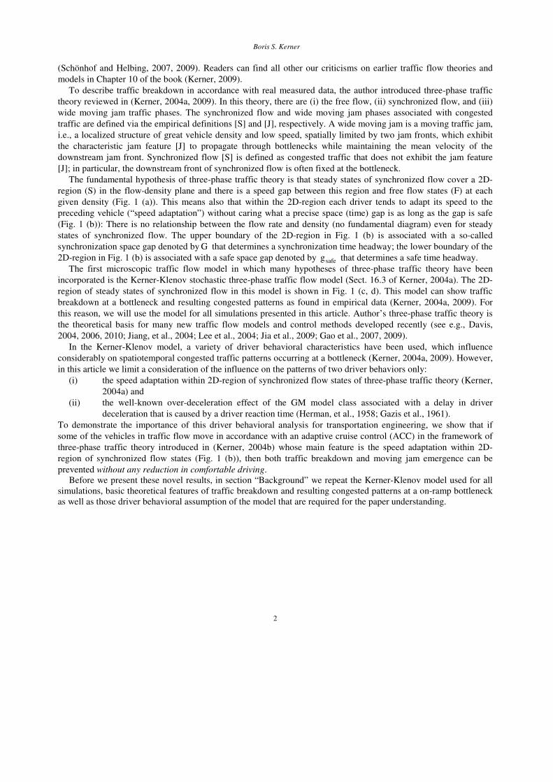
This general conclusion of three-phase traffic theory can also be seen in Fig. 9 in which three different congested

patterns occur in three realizations simulated at the same flow rates, the same vehicle and driver characteristics in

traffic flow, and the same bottleneck characteristics.

Fig. 9. Three different realizations of congested patterns associated with the same point F in the diagram shown in Fig. 7. =inq 2000

vehicles/h/lane, =onq 1000 vehicles/h.

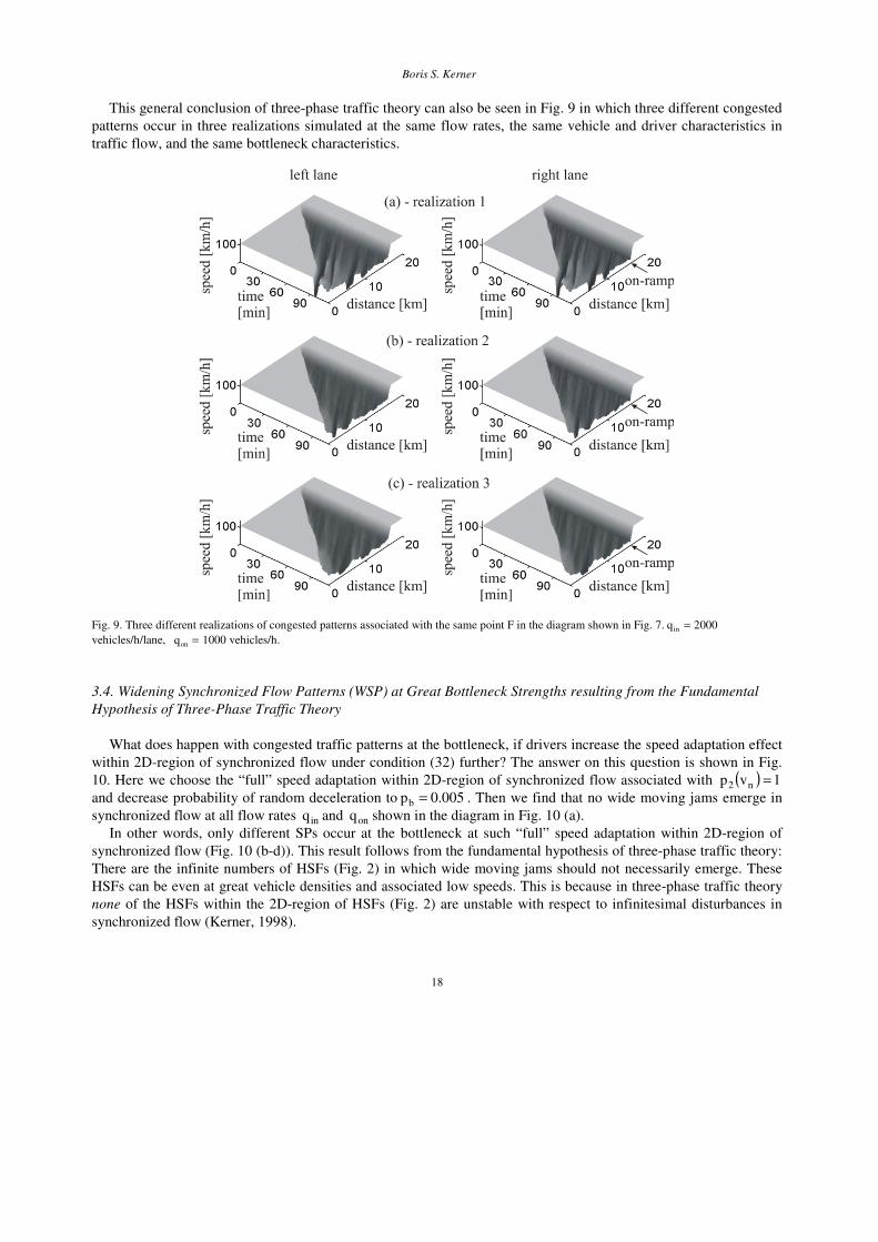
3.4. Widening Synchronized Flow Patterns (WSP) at Great Bottleneck Strengths resulting from the Fundamental

Hypothesis of Three-Phase Traffic Theory

What does happen with congested traffic patterns at the bottleneck, if drivers increase the speed adaptation effect

within 2D-region of synchronized flow under condition (32) further? The answer on this question is shown in Fig.

10. Here we choose the “full” speed adaptation within 2D-region of synchronized flow associated with ( ) 1vp n2 =

and decrease probability of random deceleration to 005.0pb = . Then we find that no wide moving jams emerge in

synchronized flow at all flow rates inq and onq shown in the diagram in Fig. 10 (a).

In other words, only different SPs occur at the bottleneck at such “full” speed adaptation within 2D-region of

synchronized flow (Fig. 10 (b-d)). This result follows from the fundamental hypothesis of three-phase traffic theory:

There are the infinite numbers of HSFs (Fig. 2) in which wide moving jams should not necessarily emerge. These

HSFs can be even at great vehicle densities and associated low speeds. This is because in three-phase traffic theory

none of the HSFs within the 2D-region of HSFs (Fig. 2) are unstable with respect to infinitesimal disturbances in

synchronized flow (Kerner, 1998).

Boris S. Kerner

19

Fig. 10. Features of congested patterns at great speed adaptation: (a-c) Congested pattern diagram (a) at ( ) 1vp n2 = and 5.0p1 = and related MSP

(b) and WSP (c). (d, e) WSP (d) and data within synchronized flow (e) at ( ) 1vp n2 = and 7.0p1 = . Other model parameters in (a-e) are the same

as those in Table 1. (f, g) GP (f) and data within synchronized flow (g) at model parameters of Table 1. In (b-d), (f) speed in space and time in

the right lane. In (b-g), =)q,q( inon (30, 2118) (b), (1400, 2105) (c), (1500, 1846) (d-g) ( vehicles/h, vehicles/h/lane). Average (30 min interval)

time headway in synchronized flow of WSP (d, e) is 2.04 s, i.e., is longer than =τ )a(jam,del 1.74 s, while for pinch region of GP (f, g) the average

time headway is about 1.39 s, i.e., it is shorter than )a(

jam,delτ .

Boris S. Kerner

20

The hypothesis about great density HSFs incorporated in the traffic flow model explains results of simulations

presented in Fig. 10 in which widening synchronized flow patterns (WSP) of a great density and low speed (e.g.,

Fig. 10(d)) appear upstream of a bottleneck. Such great density and low speed WSPs exist at great bottleneck

strengths, when speed adaptation of drivers is great enough (Fig. 10(a)): In this case, dynamic synchronized flow

within an WSP is associated mostly with stable synchronized flow states that are below the line J (Fig. 2). Thus in

three-phase traffic theory

• WSPs can occur even at heavy bottlenecks. In particular, this effect can be found when most drivers

move in synchronized flow at time headways that are longer than )a(

jam,delτ (Fig. 2). In other words,

WSPs at heavy bottlenecks can be found in real measured traffic data 3.

The importance of 2D-region of synchronized flow for the explaining of real measured data (Kerner, 2004a,

2009) is one of the basic results for the introduction by the author of “driver alike adaptive cruise control” (DA-

ACC) (Kerner, 2004b), i.e., the ACC in the framework of three-phase traffic theory briefly discussed below.

4. Driver Alike Adaptive Cruise Control (DA-ACC) – ACC in the Framework of Three-Phase Traffic Theory

4.1. Basic Operation Modes of ACC

Before we consider DA-ACC, we explain the main operation mode of a usual ACC widely used in vehicles (Fig.

11) (see references in Chap. 32 of Winner et al., 2009). The ACC-vehicle measures the space gap g and speed

difference between the preceding vehicle and ACC-vehicle vvv −=∆l

, where v is the ACC-vehicle speed, l

v is

the speed of the preceding vehicle. Based on the current values of g , v , and v∆ , the ACC vehicle calculates the

current time headway headwayτ between the ACC-vehicle and the preceding vehicle. For simplicity, we consider

here only a case in which absolute values of v∆ , the difference ACCheadway τ−τ=τ∆ (where ACCτ is a desired time

headway chosen by a driver), and acceleration (deceleration) of the preceding vehicle are not very great.

Fig. 11. Main operation mode of a usual ACC (see references in Chap. 32 of Winner et al., 2009)

Then the acceleration (deceleration) of the ACC-vehicle is given by a well-known formula:

)t(vK)g)t(g(Ka 2ACC1ACC ∆+−= , (47)

3 Up to now empirical WSP of a great density at heavy bottlenecks are not found in measured traffic data: As proven in Sect. 10.3.10 of

(Kerner, 2009), an empirical proof of homogeneous congestion made in (Schönhof and Helbing, 2007, 2009) is invalid.

Boris S. Kerner

21

where ACCg is a desired space gap (Fig. 11) related to the desired time headway ACCτ . 1K , 2K are dynamic

coefficients of ACC ( 0K,K 21 > ). The ACC should maintain v∆ close to zero and the space gap g close to ACCg ,

i.e., the time headway should be close to ACCτ . At higher speeds, ACCACC vg τ= is an increasing speed function

(Fig. 11). When 0v =∆ and ACCgg > , as follows from (47) the ACC-vehicle accelerates; otherwise, i.e., at

ACCgg < , the ACC-vehicle decelerates (Fig. 11).

4.2. Basic Operation Mode of DA-ACC

In accordance with one of the basic driver behavioral assumptions of three-phase traffic theory, when the space

gap to the preceding vehicle is within a 2D-region in the space-gap-speed plane (dashed region in Fig. 1 (b)), a

driver adapts its speed to the speed of the preceding vehicle without caring, what the precise space gap is (Kerner,

1998, 2004a). For this reason, we call an ACC with this fundamental feature of three-phase traffic theory as a driver

alike ACC (DA-ACC). Thus the basic operation mode of an DA-ACC vehicle is given by formula

safevACCDA ggGat)t(vKa ≥≥∆= ∆− (48)

associated with three-phase traffic theory: Within 2D-region in the space-gap-speed plane (dashed region in Fig. 12)

acceleration (deceleration) of the DA-ACC vehicle does not depend on the space gap, i.e., on the time headway to

the preceding vehicle at all. In other words, in contrast with the basic formula of an ACC-vehicle (47), the DA-ACC

mode (48) does not maintain a desired time headway chosen by the driver (Kerner, 2004b).

As in the Kerner-Klenov model, in (48) G and safeg are the synchronization and safe space gaps, respectively;

vK∆ is a dynamic coefficient that is greater than zero. At Gg > the DA-ACC-vehicle accelerates, whereas at

safegg < the DA-ACC-vehicle decelerates. In other words, outside of the 2D-region in the space-gap-speed plane

formula (48) is not applied. A possible variety of operation DA-ACC modes labeled in Fig. 12 as “acceleration” and

”deceleration” outside of the 2D-region are described in (Kerner, 2007).

Fig. 12. Basic operation mode of DA-ACC (Kerner, 2004b, 2007, 2009): A part of 2D-region of space gaps between a vehicle moving in

accordance with the DA-ACC mode (48) and the preceding vehicles in the space-gap-speed plane (dashed region).

4.3. Prevention of Traffic Congestion at Bottleneck through the Use of DA-ACC

Each developer of ACC knows that if dynamic coefficients 1K and 2K of ACC in (47) are chosen great enough,

then any platoon of the ACC-vehicles is stable and no moving jam emerge in traffic flow consisting only of the

Boris S. Kerner

22

ACC-vehicles. Indeed, when 1K and 2K in (47) are great enough, ACC-vehicles react very quickly on changes in

values )g)t(g( ACC− and )t(v∆ , therefore, the ACC-vehicles damp speed disturbances within the platoon.

However, such quick damping of speed disturbances at great values of 1K , 2K in (47) is very uncomfortable for

drivers. This is because the very quick damping of speed disturbances causes considerable ACC-vehicle acceleration

(deceleration) even at relatively small values )g)t(g( ACC− and )t(v∆ . For this reason, for comfortable driving

developers of real ACC have to choose relative small dynamic coefficients 1K , 2K of ACC, which cannot prevent

moving jam emerge in traffic flow (see for example Sect. 23.6.3 of Kerner, 2004a). The mentioned problem is one

the problems of ACC-vehicles leading to a conflict between the dynamic and comfortable ACC behavior.

An DA-ACC-vehicle removes this conflict and it enhances traffic flow considerably. This is because an DA-

ACC is related to a “hypothetical driver” that while approaching a slower moving preceding vehicle is able to

perform the “perfect” speed adaptation to the speed of the preceding vehicle under condition (32); in addition, this

“hypothetical driver” does not exhibit long time delays that are usual for real drivers.

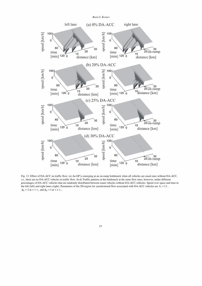
The effect of DA-ACC-vehicles on traffic flow is shown in Fig. 13. In these simulations, there are DA-ACC-

vehicles randomly distributed between vehicles without any ACC. The vehicles without ACC move in accordance

with the stochastic model of Sect. 2.2 with model parameters of Table 1.

In the simulation scenario (Fig. 13 (a)), an GP occurs spontaneously at the on-ramp bottleneck when there are no

DA-ACC-vehicles in traffic flow. When DA-ACC vehicles appear, a strong reduction in traffic congestion is

observed (Fig. 13 (b-d)). The greater the percentage of the DA-ACC vehicles is, the less the traffic congestion at the

bottleneck (Fig. 13 (b, c)). There is a critical percentage of the DA-ACC vehicles, which is about 28%: when the

percentage of the DA-ACC vehicles is greater than the critical one, no traffic breakdown and therefore no traffic

congestion occurs at the bottleneck (Fig. 13 (d)).

It must be stressed that the effect of traffic congestion avoidance through the use of DA-ACC is reached at a

small dynamic coefficient in the basic DA-ACC mode (48) 1v s14.0K −

∆ = , which is associated with a very

comfortable driving. For a comparison, to prevent moving jam emergence with a usual ACC (47), in simulations

presented in Fig. 23.18 of the book (Kerner, 2004a) the associated dynamic coefficient in (47) should

be 12 s55.0K −= related to a very uncomfortable driving.

The effect of DA-ACC vehicles on traffic flow (Fig. 13 (d)) is explained as follows. The DA-ACC vehicles do

not exhibit relatively long time delays in deceleration and acceleration that are usual for drivers. These driver time

delays are responsible both for traffic breakdown in free flow and the resulting moving jam emergence in

synchronized flow. Therefore in traffic flow without DA-ACC vehicles the GP occurs (Fig. 13 (a)), whereas in

traffic flow in which the DA-ACC vehicles dominate free flow remains (Fig. 13 (d)).

Boris S. Kerner

23

Fig. 13. Effect of DA-ACC on traffic flow: (a) An GP is emerging at an on-ramp bottleneck when all vehicles are usual ones without DA-ACC,

i.e., there are no DA-ACC vehicles in traffic flow. (b-d) Traffic patterns at the bottleneck at the same flow rates, however, under different

percentages of DA-ACC vehicles that are randomly distributed between usual vehicles without DA-ACC-vehicles. Speed over space and time in

the left (left) and right lanes (right). Parameters of the 2D-region for synchronized flow associated with DA-ACC vehicles are 5.1k = ,

ll vvat1andvvat2 00 ≥=φ<=φ .

Boris S. Kerner

24

5. Discussion

5.1. Conclusions

Simulations with a stochastic microscopic three-phase traffic flow model allow us to make the following

conclusions:

1. Drivers behaviors associated with speed adaptation to the speed of the preceding vehicle within 2D-region

of synchronized flow influence traffic congestion at a highway bottleneck considerably. When the speed

adaptation is strong enough, no wide moving jams occur in synchronized flow even at great flow rates

upstream of the bottleneck. In this case, WSPs remain at the bottleneck at great bottleneck strengths.

2. The greatest speed adaptation to the speed of the preceding vehicle within 2D-region of synchronized flow

can be realized due to the use of an ACC in the framework of three-phase traffic theory called as driver

alike ACC (DA-ACC). The simulations of DA-ACC behavior explain the following advantages of the DA-

ACC (48) based on three-phase traffic theory in comparison with the usual ACC (47):

• The removing of a conflict between the dynamic and comfortable ACC behavior. In particular, a much

comfortable vehicle motion in congested traffic is possible.

• DA-ACC-vehicles can prevent traffic breakdown at a bottleneck and wide moving jam emergence in

synchronized flow.

• As well-known, under congestion fuel consumption increases; therefore, the DA-ACC that decreases

speed disturbances in traffic flow and prevents congestion can lead to reduction in fuel consumption

and 2CO emissions.

5.2. Criticism of “Criticism of Three-Phase Traffic Theory”

Three-phase traffic theory is an alternative theory to well-known and widely accepted earlier traffic flow theories

and models reviewed in (May, 1090; Leutzbach, 1998; Gartner et al, 2001; Chowdhury, et al, 2000; Helbing, 2001;

Nagatani, 2002; Nagel, et al, 2003; Mahnke, et al, 2005; Rakha, et al, 2009). Recently, this theory has been

criticized in (Schönhof and Helbing, 2007, 2009). Author’s responses to these criticisms have already been done in

Sect. 10.3 of (Kerner, 2009). Nevertheless, for a deeper understanding of the article results, we make more detailed

explanations of some of these critical responses on (Schönhof and Helbing, 2007, 2009) below.

5.2.1. Traffic breakdown: F → S transition

The main criticism made in three-phase traffic theory (Kerner, 2004a, 2009) on the earlier traffic flow theories

including traffic flow models of the group of Helbing (Helbing, 2001; Schönhof and Helbing, 2007, 2009), which

explain traffic breakdown by free flow instability (Gazis, 1961; May, 1090; Leutzbach, 1998; Gartner et al, 2001;

Chowdhury, et al, 2000; Nagatani, 2002; Nagel, et al, 2003; Mahnke, et al, 2005; Rakha, et al, 2009), is that this free

flow instability is responsible for wide moving jam formation in free flow (F → J transition). In contrast, traffic

breakdown observed in real measured data is governed by a first-order F → S transition (Kerner, 2004a, 2009).

In (Schönhof and Helbing, 2007, 2009), an empirical observation of a “boomerang effect”, i.e., “growing

perturbations on a homogeneous freeway section without on- and off-ramps” (see caption to Figure 1 of Schönhof

and Helbing, 2007) that should lead to wide moving jam emergence in free flow has been stated. It must be stressed

that the term boomerang effect has a sense only when traffic breakdown occurs without influence of a bottleneck.

Otherwise, if a bottleneck is the reason for traffic breakdown and the resulting upstream congestion propagation,

then this well-known and usual way of the congestion occurrence has nothing to do with the boomerang effect. This

“boomerang effect” should prove that a spontaneous F → J transition might govern traffic breakdown in free flow.

This should be one of the criticisms of three-phase traffic theory in which rather the spontaneous F → J transition a

sequence of F → S → J transitions governs the spontaneous wide moving jam emergence (Kerner, 1998).

Boris S. Kerner

25

However, as proven in (Kerner and Klenov, 2009) based on the same measured traffic data as that used in

(Schönhof and Helbing, 2007, 2009) in this data rather than the “boomerang effect, an F → S transition occurs at an

off-ramp bottleneck resulting in moving SP (MSP) formation; later, due to an S → J transition within the MSP it

transforms into a wide moving jam. Thus in the empirical data wide moving jams emerge due to sequence of

F → S → J transitions, i.e., the study of (Schönhof and Helbing, 2007, 2009) is invalid. A more detailed

consideration of the “boomerang effect” in free flow and the associated criticism of these empirical studies can be

found in Sect. 10.3.7 of the book (Kerner, 2009).

5.2.2. Proof of criticism of HCT and OCT model solutions as well as diagram of congested patterns of Helbing,

Treiber et al

In some traffic flow models in the framework of the fundamental diagram hypothesis, the density region at the

fundamental diagram, within which traffic flow is unstable (dashed curve in Fig. 14 (a)), is limited at greater

densities: At the densities )HCT(crρ≥ρ states on the fundamental diagram are stable with respect to small disturbances.

These stable homogeneous in space and time model solutions of a great density, which can appear upstream of a

bottleneck in simulations of these models, have been called as HCT in (Helbing, et al, 1999; Treiber, et al, 2000;

Helbing, 2001).

In (Kerner, 2004a), the application of HCT model solutions for explanations of real measured data made in

(Helbing, 2001; Treiber, et al, 2000) has been criticized. Below based on numerical simulations of features of HCT

model solutions, we prove this criticism and show that

• the HCT model solutions, which are the basic solutions for the theoretical diagrams of congested

patterns derived by Helbing, Treiber et al. (Helbing, et al, 1999; Treiber, et al, 2000, 2010; Helbing,

2001; Schönhof and Helbing, 2007, 2009; Helbing et al., 2009), have no sense for real traffic.

To prove that the HCT model solutions have no sense for real traffic flow, we should note that in all known

empirical observations, the downstream front of a wide moving jam propagates through any dense congested traffic

and bottlenecks while maintaining the mean velocity of the front gv . In other words, this empirical feature [J] of

wide moving jams is independent of the state of traffic flow downstream of the jam.

However, traffic flow models with the HCT model solutions cannot satisfy this very important characteristic

empirical feature of traffic. To illustrate this, we consider features of wide moving jam propagation in these models

with an example of the fundamental diagram shown in Fig. 14 (a). We find that the characteristic jam feature [J] in

these models is satisfied when free flow is downstream of the jam (wide moving jam labeled by “jam A” in Fig. 14

(c, d)). In contrast, the jam feature [J] does not remain when an HCT model solution is downstream of a wide

moving jam (the jam labeled by “jam B”). This is because rather than the line J, the downstream front of the “B”

propagates with a negative velocity )HCT(

gv that is associated with a line )HCT(

J in the flow-density plane between

the state within the jam with the jam density maxρ and a point at the fundamental diagram for an HCT solution (with

a density )HCT(ρ in Fig. 14 (b)). As a result, the absolute value of the downstream front velocity of the “jam A” gv

is considerably greater than the one for the “jam B” )HCT(gv . Moreover, the greater the density

)HCT(ρ of the HCT,

the smaller )HCT(gv . As abovementioned, this is inconsistent with measured traffic data of wide moving jam

propagation. This proves that HCT model solutions of Ref. (Helbing, 2001; Helbing, et al, 1999; Treiber, et al, 2000,

2010; Schönhof and Helbing, 2007, 2009; Helbing et al., 2009) are not consistent with the empirical feature [J] of

wide moving jam propagation through any dense congested traffic while maintaining the mean velocity of the jam

front. For this reason, the features of these HCT model solutions have no sense for real traffic flow.

Due to the existence of HCT model solutions, these traffic flow models exhibit also model solutions called

oscillating congested traffic (OCT) (Helbing, et al, 1999; Helbing, 2001; Treiber, et al, 2000, 2010; Schönhof and

Helbing, 2007, 2009; Helbing et al., 2009). An OCT model solution appears in these models due to the existence of

the critical density )HCT(crρ for an instability of HCT: When the density in HCT decreases and this HCT density

approaches the critical density )HCT(crρ (Fig. 14 (a)), then due to HCT instability, OCT model solution occurs. Thus

we can make the conclusions:

Boris S. Kerner

26

1. OCT model solutions of (Helbing, et al, 1999; Helbing, 2001; Treiber, et al, 2000, 2010; Schönhof and

Helbing, 2007, 2009; Helbing et al., 2009) appear as a result of the instability of HCT model solutions in

traffic flow models with the fundamental diagram shown in Fig. 14(a).

2. As proven above, HCT model solutions of these models have no sense for real traffic. Therefore, the

OCT model solutions resulting from HCT as well as theoretical congested patterns consisting of HCT

and OCT combinations have also no relation to real traffic.

3. HCT and OCT model solutions are important elements of diagrams of congested patterns at bottlenecks

of (Helbing, et al, 1999; Helbing, 2001; Treiber, et al, 2000, 2010; Schönhof and Helbing, 2007, 2009;

Helbing et al., 2009). This is one of the reasons why these theoretical diagrams have no sense and,

therefore, no application to real traffic.

Fig. 14. Simulations of HCT model solutions and wide moving jam propagation: (a) Fundamental diagram with HCT (b) Fundamental diagram

of (a) together with the lines J and )HCT(J that represent in the flow--density plane the downstream fronts of two wide moving jams denoted by

“jam A” and “jam B”, respectively in (c, d). (c, d) Propagation of two wide moving jams when downstream of the jams either free flow (“jam

A”) or HCT (“jam B”) occur, respectively; speed (b) and density (c) in space and time. Payne-like model. Taken from (Kerner, 2009).

5.2.3. Criticism of explanations of empirical congested patterns through spatiotemporal combinations of HCT and

OCT model solutions

We should note that in simulations of non-linear traffic flow models of (Treiber, et al, 2000, 2010; Schönhof and

Helbing, 2007, 2009), a diverse variety of spatiotemporal combinations of the HCT and OCT model solutions can be

Boris S. Kerner

27

found. Through an appropriate choice of boundary and initial conditions used in simulations, some of these HCT

and OCT combinations look like real measured spatiotemporal congested patterns. This visible similarity between

the HCT and OCT combinations and real patterns has been used in (Helbing, 2001; Helbing, et al, 1999; Treiber, et

al, 2000, 2010; Schönhof and Helbing, 2007, 2009) for the statement that traffic flow models of these authors can

describe features of real traffic.

Fig. 15. Simulations of HCT and OCT combinations that occur at downstream on-ramp ( =x 20 km) and upstream off-ramp ( =x 16 km)

bottlenecks: (a) Fundamental diagram taken from Fig. 14(a) in which three points 1, 2, and 3 are marked related to different vehicle densities in

congested traffic. (b) HCT upstream of the on-ramp bottleneck related to point 1 in (a) for density )HCT(cr1 ρ>ρ when the flow rate to the off-

ramp =offq 0. (c) Appearance of OCT upstream of the off-ramp due to instability of HCT upstream of the off-ramp caused by >= 1offoff qq 0

associated with point 2 on the fundamental diagram in (a). (d, e) Stronger growth of OCT upstream of the off-ramp due to increase in the flow

rate to the off-ramp to 1off2off qq > associated with point 3 on the fundamental diagram in (a); in (d, e) the same pattern in different scales is

shown. In (b-e), vehicle speed in space and time. Simulations of Payne-like model.

Boris S. Kerner

28

For example, such HCT and OCT combination occurs in simulations of traffic on a road with two adjacent

bottlenecks: downstream on-ramp and upstream off-ramp bottlenecks (Schönhof and Helbing, 2007, 2009).

Firstly, if the on-ramp inflow is great enough and the off-ramp outflow offq is zero, the density in congested

traffic 1ρ upstream of the on-ramp can be greater than the critical density )HCT(crρ (point 1 in Fig. 15(a)). This results

in a HCT model solution upstream of the on-ramp (Fig. 15(b)). As proven in Sect. 5.2.2 above, the HCT has no

sense for real traffic.

Now we choose >offq 0. Due to the off-ramp outflow >offq 0, the flow rate increases and density decreases

within this HCT upstream of the off-ramp. As the result, point on the fundamental diagram related to HCT upstream

of the off-ramp moves to smaller densities. Specifically, at chosen model parameters point 1 moves to point 2 on the

fundamental diagram. However, point 2 is related to the density )HCT(cr2 ρ<ρ , which is on a part of the fundamental

diagram for unstable model solutions (a dashed part of the fundamental diagram in Fig. 15(a) left to the critical

density )HCT(crρ ). For this reason, the HCT becomes unstable upstream of the off-ramp and transforms into OCT

upstream of the off-ramp: HCT and OCT combination occurs spontaneously (Fig. 15(c)).

In a neighborhood of the critical density )HCT(crρ for HCT instability, the smaller the density in congested traffic

in comparison with )HCT(crρ , the greater the increment of the growth of fluctuations in the unstable model solutions

on the fundamental diagram. As a result, we find that OCT grows quicker upstream of the off-ramp (Fig. 15(d)),

when we increase offq and, therefore, point 2 on the fundamental diagram in Fig. 15(a) moves to point 3 associated

with a smaller density 3ρ ( 23 ρ<ρ ) on the fundamental diagram.

Thus the resulting simulated patterns consist of the HCT solution between the on- and off-ramp bottlenecks and

the OCT solution upstream of the off-ramp (Fig. 15(c, d)). Such spatiotemporal combinations of the HCT and OCT

model solutions, which look like as GPs (this can be clear seen when we show the pattern in Fig. 15(d) in a greater

scale (Fig. 15(e)), have been presented in (Schönhof and Helbing, 2007, 2009; Treiber, et al, 2010) as an explanation

of measured congested patterns. However, the simulated patterns contain HCT model solutions whose features have

no sense for real traffic.

• Thus any explanation of real measured spatiotemporal congested patterns through the use of

combinations HCT and OCT model solutions made in (Helbing, 2001; Treiber, et al, 2000, 2010;

Schönhof and Helbing, 2007, 2009) is invalid.

5.2.4. Conclusions to criticism of three-phase traffic theory

(1) Main criticisms of three-phase traffic theory are based on invalid analyses of measured traffic data made in

(Treiber, et al, 2000, 2010; Schönhof and Helbing, 2007, 2009), in particular, resulting in the incorrect statement

about empirical observations of the “boomerang effect”, i.e., an F → J transition in real measured traffic data.

(2) Three-phase traffic theory explains real measured spatiotemporal congested patterns through features of SPs

and GPs found in this theory (Kerner, 2004a, 2009). Alternative explanations of the same measured congested

patterns through the use of diverse combinations of HCT and OCT model solutions made in (Helbing, 2001;

Treiber, et al, 2000, 2010; Schönhof and Helbing, 2007, 2009) are considered as additional criticisms of three-phase

traffic theory. As proven above, features of HCT model solutions have no sense for real traffic. Therefore,

spatiotemporal combinations of the HCT and OCT solutions as well as the associated theoretical diagrams of

congested patterns of (Helbing, 2001; Helbing, et al, 1999; Treiber, et al, 2000, 2010; Schönhof and Helbing, 2007,

2009) are not applicable for real traffic flow. In other words, the associated criticisms of three-phase traffic theory

are also incorrect.

Boris S. Kerner

29

Acknowledgements:

I thank Sergey Klenov for discussions and help in numerical simulations.

References

M. Bando, K. Hasebe, A. Nakayama, A. Shibata, Y. Sugiyama (1995). Dynamical model of traffic congestion and numerical simulations.

Phys. Rev. E 51, 1035-1042.

R. Barlovic’, L. Santen, A. Schadschneider, M. Schreckenberg (1998). Metastable states in cellular automata for traffic flow. Eur. Phys. J. B 5,

793-800.

M. Brackstone, M. McDonald (1998). Car-following: a histirical review. Transp. Res. F, 2, 181-196.

D. Chowdhury, L. Santen, A. Schadschneider (2000). Statistical physics of vehicular traffic and some related systems. Physics Reports 329, 199.

M. Cremer (1979). Der Verkehrsfluss auf Schnellstrassen (Springer, Berlin).

C.F. Daganzo (1997). Fundamentals of Transportation and Traffic Operations (Elsevier Science Inc., New York).

L.C. Davis (2004). Multilane simulations of traffic phases. Phys. Rev. E 69, 016108.

L.C. Davis (2006). Controlling traffic flow near the transition to the synchronous flow phase. Physica A, 368, 541-550.

L.C. Davis (2010). Predicting travel time to limit congestion at a highway bottleneck. Physica A, 389, 3588-3599.

D. Drew (1968). Traffic Flow Theory and Control (McGraw Hill, New York).

K. Gao, R. Jiang, S-X. Hu, B-H. Wang, Q.S. Wu (2007). Cellular-automaton model with velocity adaptation in the framework of Kerner's three-

phase traffic theory. Phys. Rev. E 76, 026105.

K. Gao, R. Jiang, B-H. Wang, Q.S. Wu (2009). Discontinuous transition from free flow to synchronized flow induced by short-range interaction

between vehicles in a three-phase traffic flow model. Physica A 388, 3233-3243.

D.C. Gazis (2002). Traffic Theory (Springer, Berlin).

D.C. Gazis, R. Herman, R.W. Rothery (1961). Nonlinear follow the leader models of traffic flow. Operations Res. 9, 545-567.

N.H. Gartner, C.J. Messer, A. Rathi (eds.) (2001). Traffic Flow Theory: A State-of-the-Art Report (Transportation Research Board, Washington,

D.C.).

P.G. Gipps (1981). Behavioral Car-Following Model for Computer Simulation. Trans. Res. B. 15, 105-111.

P.G. Gipps (1986). A model for the structure of lane-changing decisions. Trans. Res. B. 20, 403-414.

F.A. Haight (1963). Mathematical Theories of Traffic Flow (Academic Press, New York).

D. Helbing (2001). Traffic and related self-driven many-particle systems. Rev. Mod. Phys. 73, 1067-1141.

D. Helbing, A. Hennecke, M. Treiber (1999). Phase Diagram of Traffic States in the Presence of Inhomogeneities. Phys. Rev. Lett. 82, 4360-

4363.

D. Helbing, M. Treiber, A. Kesting, and M. Schönhof (2009). Theoretical vs. empirical classification and prediction of congested traffic states.

Eur. Phys. J. B, 69, 583-598.

R. Herman, E.W. Montroll, R.B. Potts, R.W. Rothery (1959). Traffic Dynamics Analysis of Stability in Car-Following, Operations Res. 7, 86-

106.

Highway Capacity Manual 2000 (National Research Council, Transportation Research Board, Washington, D.C.).

B. Jia, X-G. Li, T. Chen, R. Jiang, Z-Y. Gao (2009). Cellular automaton model with time gap dependent randomization under Kerner's three-

phase traffic theory. Transportmetrica (on-line 1944-0987).

R. Jiang, Q.S. Wu (2004). Spatial–temporal patterns at an isolated on-ramp in a new cellular automata model based on three-phase traffic theory.

J. Phys. A: Math. Gen. 37, 8197—8213.

B.S. Kerner (1998). Experimental Features of Self-Organization in Traffic Flow. Phys. Rev. Lett. 87, 3797-3800.

B.S. Kerner (1999). Congested traffic flow: Observations and Theory. Transportation Research Record 1678, 160-167.

B.S. Kerner (2004a). The physics of traffic (Springer, Berlin).

B.S. Kerner (2004b). Method for actuating a traffic-adaptive assistance system which is located in a vehicle. German patent publication DE

10308256 A1; EU Patent EP 1597106 B1 (2005); USA patent US 20070150167 (2007),

http://www.freepatentsonline.com/20070150167.html.

B.S. Kerner (2007). Traffic-adaptive assistance system. German patent publications DE 102005017559, DE 102005017560, DE 102005033495,

DE 102007008253, DE 102007008254, DE 102007008255, DE 102007008257.

B.S. Kerner (2009). Introduction to modern traffic flow theory and control (Springer, Berlin)

B.S. Kerner and S.L. Klenov (2009). Phase transitions in traffic flow on multi-lane roads. Phys. Rev. E, 80, 056101.

S. Krauss, P. Wagner, C. Gawron (1997). Metastable states in a microscopic model of traffic flow. Phys. Rev. E 55, 5597—5602.

W. Leutzbach (1988). Introduction to the Theory of Traffic Flow (Springer, Berlin).

Boris S. Kerner

30

H.K. Lee, R. Barlović, M. Schreckenberg, D. Kim (2004). Mechanical Restriction versus Human Overreaction Triggering Congested Traffic

States. Phys. Rev. Lett. 92, 238702.

R. Mahnke, J. Kaupuźs, I. Lubashevsky (2005). Probabilistic description of traffic flow. Phys. Rep. 408, 1-130.

A.D. May (1990) Traffic Flow Fundamentals (Prentice-Hall, Inc., New Jersey).

K. Nagel, M. Schreckenberg (1992). A cellular automaton model for freeway traffic. J. Phys. (France) I 2, 2221-2229.

K. Nagel, P. Wagner, R. Woesler (2003). Still Flowing: Approaches to Traffic Flow and Traffic Jam Modeling. Operation Res. 51, 681-716.

G.F. Newell (1982). Applications of Queuing Theory (Chapman Hall, London)

G.F. Newell (1961). A simplified car-following theory: a lower order model. Oper. Res. 9, 209-229.

T. Nagatani (2002). The physics of traffic jams. Rep. Prog. Phys. 65, 1331-1386.

M. Papageorgiou (1983). Application of Automatic Control Concepts in Traffic Flow Modeling and Control (Springer, Berlin, New York).

I. Prigogine, R. Herman (1971). Kinetic Theory of Vehicular Traffic (American Elsevier, New York).

H. Rakha, P. Pasumarthy, S. Adjerid (2009). A Simplified Behavioral Vehicle Longitudinal Motion Model. Transportation Letters, 1, 95-110.

M. Schönhof and D. Helbing (2007). Empirical features of Congested Traffic States and their Implications for Traffic Modeling. Transp. Sc. 41,

135—166.

M. Schönhof and D. Helbing (2009). Criticism of three-phase traffic theory. Transp. Rec. B, 43, 784-797.

M. Treiber, A. Hennecke, D. Helbing (2000). Congested traffic states in empirical observations and microscopic simulations. Phys. Rev. E 62,

1805—1824.

M. Treiber, A. Kesting, D. Helbing (2010). Three-phase traffic theory and two-phase models with a fundamental diagram in the light of empirical

stylized facts. Transportation Research Part B: Methodological, 44, 983-1000. Doi: 10.1016/j.trb.2010.03.004.

G.B. Whitham (1974). Linear and Nonlinear Waves (Wiley, New York).

R. Wiedemann (1974). Simulation des Verkehrsflusses (University of Karlsruhe, Karlsruhe, Germany).

H. Winner, S. Hakuli, G. Wolf (editors) (2009). Handbuch Fahrerassistenzsysteme (Vieweg + Teubner Verlag, Wiesbaden, Germany).