effect of drilling-mud base-oil contamination on crude...

SPWLA 46th Annual Logging Symposium, June 26-29, 2005

EFFECT OF DRILLING-MUD BASE-OIL CONTAMINATION ON CRUDE OIL T2 DISTRIBUTIONS

A. Kurup and G. J. Hirasaki, Rice University

Copyright 2005, held jointly by the Society of Petrophysicists and Well Log Analysts (SPWLA) and the submitting authors. This paper was prepared for presentation at the SPWLA 46th Annual Logging Symposium held in New Orleans, Louisiana, United States, June 26-29, 2005.

1

ABSTRACT Oil-based drilling fluids can invade formations and contaminate crude oils, hindering logging analysis. This work details 1H NMR T2 measurements with mixtures of one drilling-fluid base oil, NovaPlus (SNP), and crude oils to determine the effect of the contamination. Measurements are made using 2 MHz MARAN bench-top instruments on mixtures having various concentrations of SNP, with each of three crude oils (labeled STNS, SMY, and PBB), whose viscosities range from 13.7 to 207 cp. T2 measurements for mixtures containing SMY and SNP are repeated four times for purpose of statistical analysis. Two approaches are explored to better relate NMR measurements with contamination. In the first approach, a selective contamination index (SCI) is defined that relates the T2 distribution to the contamination. Here, a subset of the T2 data is chosen for analysis based on sensitivity to contamination. In the second approach, the T2 data are fit to a four-parameter, skewed Gaussian model for T2 distributions. Two parameters of the model are combined in a distribution parameter index (DPI), which can be related to contamination. Both the SCI and DPI values can be fit using cubic polynomials, resulting in a functional dependence on concentration. The polynomial functions, used in reverse, yield estimations of the degree of contamination, which for SMY-SNP mixtures are compared to standard T2,LM methods. The comparison of the T2,LM, SCI, and DPI methods is done in terms of the estimated error in the degree of contamination. The SCI method provides the best estimate of contamination. MOTIVATION AND APPROACH Oil wells are often drilled with the aid of oil-based fluids. During the drilling process, an oil-based mud

(OBM) is formed from the mixture of drilling fluid and drill cuttings. Filtrates from these oil-based muds invade oil-bearing formations and mix with crude oils. OBM filtrates alter the properties of the crude oils with which they mix. In NMR well logging, one concern is whether the measured T2 relaxation time distribution (or T2 distribution) changes enough to affect the estimated viscosity, which can be derived from these measurements through existing correlations. Such concerns are particularly valid because OBM filtrates are similar in molecular structure to the crude oils themselves. This inhibits attempts to separate the OBM filtrate signal from the crude oil signal in NMR logs. Other works have addressed using NMR to investigate OBM contamination of crude oils, mostly in the context of the pumpout phase of downhole fluid sampling. Bouton, et al. (2001) developed a sharpness parameter to characterize T1 relaxation times of mixtures of crude oils and base oils. Base oils are the predominant component in OBM filtrates. The sharpness parameter is at a maximum for the base oil alone and decreases monotonically for higher concentrations of crude oil. Continuing this work, Masak, et al. (2002) use a downhole fluid sampler to characterize contamination by measuring T1 relaxation times during the pumpout process. Here, measurements occur as time progresses, and the change in measured signal amplitudes is used to characterize the contamination. More recently, Akkurt, et al. (2004) have extended the analysis by developing time and T2 domain approaches to assess contamination from the pumpout phase in the application of the downhole fluid sampler. In the present work, new approaches to study contamination are developed based on the following fluids. NovaPlus, a commonly used base oil in drilling, is the contaminant. NovaPlus (3 cp) is a mixture of 16- to 18-carbon internal olefins. Nova Plus will be abbreviated as SNP. The crude oils used are from the North Sea (13.7 cp), from offshore China (207 cp), and from the Gulf of Mexico (18.7 cp). Henceforth, the crude oils will be called STNS, PBB, and SMY, respectively. The above information is summarized in Table 1. The objective in this study is to relate the degree of contamination to features in the T2 distributions. Another goal is estimating the extent of contamination


from measured T2 distributions of samples at unknown degrees of contamination. The traditional approach in studying fluids in NMR logs is using a logarithmic-mean T2 (log-mean T2, T2,LM). The new approaches are compared with using T2,LM to estimate contamination. Table 1: Viscosities and Abbreviations for Fluids Investigated

Fluid Type Abbreviation Viscosity (cp)

Nova Plus Base oil SNP 3.3

North Sea Crude oil STNS 13.7

Offshore China

Crude oil PBB 206.7

Gulf of Mexico

Crude oil SMY 18.7

2

Two new approaches will be described and implemented herein. In one approach, contamination is characterized by amplitudes at a limited range of relaxation times in each T2 distribution. In contrast, the default approach using T2,LM agglomerates data at all T2 into a weighted average. Thus, using a limited range of relaxation times from the T2 distribution would increase NMR sensitivity to contamination. This would salvage information from useful regions of the T2 distribution, without needing to consider the entire distribution as in T2,LM. The second approach uses a hypothesized probability distribution to fit the experimental T2 distribution. Data in the T2 domain are fit to a skewed Gaussian distribution, whose parameters can be related to contamination. With either of the two approaches, a polynomial fit extends the characterization over the entire contamination range. The polynomial can then be used to estimate the degree of contamination. EXPERIMENTAL The experimental samples are as follows. Crude oil mixtures with the model contaminant, NovaPlus, were prepared at various volumetric concentrations. The concentrations used for STNS and PBB mixtures are 10, 20, 50 and 75% SNP. The crude oil (0% SNP) and SNP (100% SNP) were also included in the measurements. For mixtures of SMY and SNP, concentrations prepared were 0, 10, 20, 50, 80, 90, and 100% SNP. For 20% and 50% SNP, two samples were prepared to assess reproducibility. The following measurements were performed. For all but the second samples of SMY mixtures at 20% and 50% SNP, the T2 relaxation time and the viscosity are

measured. For the two samples mentioned, the T2 relaxation time was measured but the sample volume was too low to do the viscosity measurement. Deoxygenation, the removal of the paramagnetic contaminant oxygen, was not performed before any of the T2 measurements for two reasons. First, invading base oil in a drilled formation would contain oxygen (Chen et al. 2004). Furthermore, the amount of dissolved oxygen is expected to play only a small role because the relaxation time distributions for the base and crude oils in this study fall below 1 second, for which the effect of oxygen on T2 distributions is minimal (Lo 1999). T2 measurements are made by two 2 MHz MARAN instruments, labeled MARAN-SS and MARAN-M, manufactured by Resonance Instruments. In this measurement, the decay in signal amplitude, or magnetization, is measured as a function of time. The resultant data is said to be in the time domain. The decay process is characterized by the following equation:

∑−

=j

Tt

j

jeMtM 2

0)( . (1)

In this expression, M is the total magnetization at time t, M0,j is the initial magnetization of component j, and T2,j is the T2 value corresponding to component j. The acquired data is then processed, converting the time-domain data to the T2-domain. Before this, the large number of time-domain data points is parsed. This process, called “sampling and averaging”, reduces the computational load in the conversion with minimal sacrifice to data quality (Chuah 1996). The resultant amplitudes in the T2 domain are placed at predetermined relaxation times, which are spaced apart equally in logarithmic scale. These chosen individual T2 values, T2,i, at which amplitudes are placed, are called bins. An amplitude corresponding to these bins are given the symbol, Ai. The index j is used for the time domain and index i is used for the T2 domain to signify that bins chosen do not match the intrinsic T2 values for the mixture components in general. The number of runs performed for each set of mixtures differs depending on the crude oil. For mixtures containing STNS or PBB, one T2 distribution measurement is done. For the SMY mixtures, four separate T2-distribution measurements of the same set of samples are made, for the statistical analysis below. The separate measurements will be called Run 1, Run 2, Run 3, and Run 4.


NMR data were obtained using the following conditions. Runs 1, 2, and 3 were performed with MARAN-SS and Run 4 was performed with MARAN-M. In experiments for the mixtures mentioned above, the acquisition conditions used are 128 scans, 9216 (9k) echoes (time-domain data points), 320 µs echo spacing (time between echoes in each scan), and a 5 s wait time between neighboring scans. The only exception to this is that for Run 3 and Run 4, the number of scans was not 128, but was adjusted such that the signal-to-noise ratio is 100. Data acquisition software automatically determines the actual number of scans. The viscosities are measured using a Brookfield viscometer, Model LVDV-III+. Measurements are made near the maximum shear rate that does not exceed torque limits or the rotation speed of the instrument. For the STNS and PBB mixtures, the viscosity for each set was measured after the T2 distribution was obtained. For the SMY samples, only samples having enough volume had their viscosity measured. This measurement was done after Run 1. The temperature of both T2 relaxation time measurements and viscosity measurements is 30 ºC.

3

OVERVIEW OF APPROACH The results will be divided into three approaches. The first approach is traditional, characterizing mixture viscosity and log-mean T2. The second approach applies a selective contamination index (SCI) for relating measured T2 distributions to contamination. The third approach shows how a skewed Gaussian model for the relaxation time distributions performs in estimating contamination. Before proceeding, a brief explanation as to the difference in the methods used for the T2,LM approach, the SCI approach, and the distribution parameter approach is warranted. Using T2,LM involves a one-stage analysis. All the data contributes to T2,LM. The value of T2,LM equally involves all bins, depending only on the signal amplitudes in all the bins. The methods in the SCI approach and distribution parameter approach involve two stages. The two stages in the SCI approach and the distribution parameter approach are described below. In the first stage of the SCI approach, a subset of the available T2 bins is used to define intermediate quantities, called binwise contamination indices. The second stage creates a quantity, the selective contamination index or SCI, from a function of these intermediate quantities. For the distribution parameter approach all the data is used, similar to using T2,LM. However, the approach is

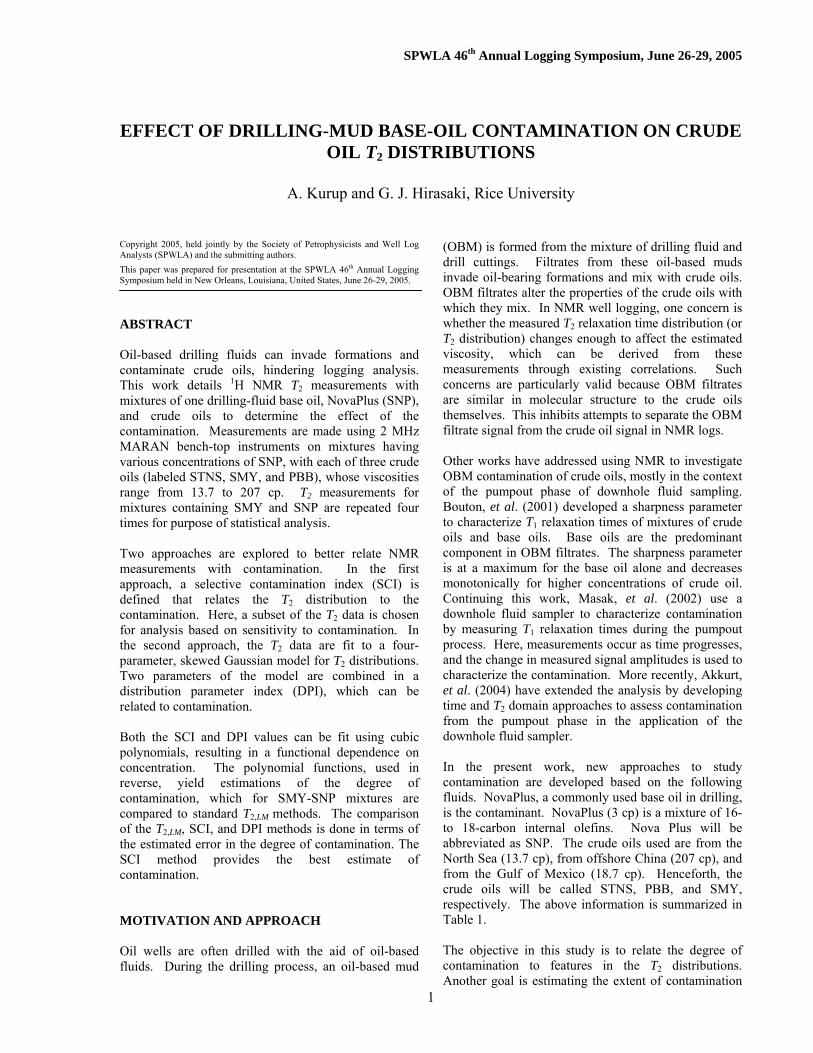
still in two stages. In the first stage, one obtains the parameters of the skewed Gaussian model used to fit the data. The second stage defines a single figure, the distribution parameter index (DPI), which is a function of a subset of these parameters. PRELIMINARY MEASUREMENTS Fig. 1 shows the incremental T2 distributions (as opposed to cumulative distributions) for mixtures of STNS and SNP. The plots represent data from 50 T2 bins. The top panel shows the distribution for the contaminant SNP, and subsequent panels contain increasing amounts of STNS. For a light crude oil like STNS, the mode, or T2 value corresponding to the highest amplitude in the distribution, does not differ greatly from the base oil, SNP. As SNP contamination decreases, the most noticeable change is that the T2 distribution becomes more skewed toward shorter relaxation times. However, much of the amplitude for all contamination levels is localized at relatively high relaxation times.

0.02.04.06.08.0

0.1 1 10 100 1000

0.01.02.03.04.05.0

0.1 1 10 100 1000

0.01.02.03.0

4.0

0.1 1 10 100 1000

0.00.51.01.52.02.5

0.1 1 10 100 1000

0.00.5

1.01.5

2.0

0.1 1 10 100 1000

0.00.51.01.52.0

0.1 1 10 100 1000

Relaxation Time (ms)

Ampl i t ude

SNP

75% SNP

50% SNP

20% SNP

10% SNP

STNS

STNS Mixtures

Figure 1: Stacked plots showing incremental T2 relaxation time distributions for mixtures of STNS crude oil and SNP base oil. Note that the amplitude axis is not to scale for all curves in the stack.


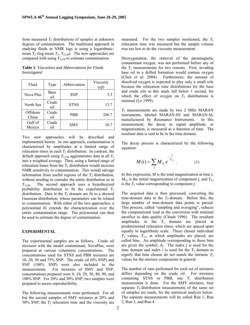
The situation is different for PBB mixtures, Fig. 2. Fig. 2 shows T2 distributions for mixtures in the same format as for Fig. 1. In these mixtures, all measured contamination levels can be differentiated. Both the mode and the tail of the distribution shift noticeably as the contamination level changes. These features are seen even at a contamination of 10% SNP.

0.02.04.06.08.0

0.1 1 10 100 1000

0.01.0

2.03.04.0

0.1 1 10 100 1000

0.00.51.01.52.02.5

0.1 1 10 100 1000

0.00.51.01.52.0

0.1 1 10 100 1000

0.0

0.5

1.0

1.5

0.1 1 10 100 1000

0.0

0.5

1.0

1.5

0.1 1 10 100 1000

A m p l i t u d e


SNP

PBB

75% SNP

50% SNP

20% SNP

10% SNP

PBB Mixtures

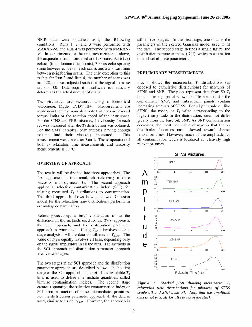
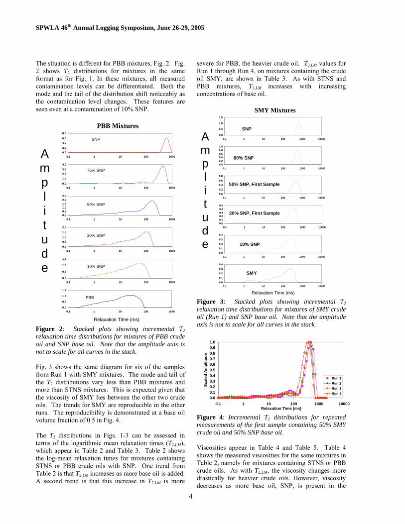
Figure 2: Stacked plots showing incremental T2 relaxation time distributions for mixtures of PBB crude oil and SNP base oil. Note that the amplitude axis is not to scale for all curves in the stack. Fig. 3 shows the same diagram for six of the samples from Run 1 with SMY mixtures. The mode and tail of the T2 distributions vary less than PBB mixtures and more than STNS mixtures. This is expected given that the viscosity of SMY lies between the other two crude oils. The trends for SMY are reproducible in the other runs. The reproducibility is demonstrated at a base oil volume fraction of 0.5 in Fig. 4. The T2 distributions in Figs. 1-3 can be assessed in terms of the logarithmic mean relaxation times (T2,LM), which appear in Table 2 and Table 3. Table 2 shows the log-mean relaxation times for mixtures containing STNS or PBB crude oils with SNP. One trend from Table 2 is that T2,LM increases as more base oil is added. A second trend is that this increase in T2,LM is more

severe for PBB, the heavier crude oil. T2,LM values for Run 1 through Run 4, on mixtures containing the crude oil SMY, are shown in Table 3. As with STNS and PBB mixtures, T2,LM increases with increasing concentrations of base oil.

SNP0.0

0.5

1.0

1.5

0.1 1 10 100 1000 10000

80% SNP0.00.20.40.60.81.0

0.1 1 10 100 1000 10000

50% SNP, First Sample

0.00.20.40.60.8

0.1 1 10 100 1000 10000

20% SNP, First Sample

0.00.10.20.30.40.5

0.1 1 10 100 1000 10000

10% SNP0.00.10.20.30.4

0.1 1 10 100 1000 10000

SMY

0.00.10.20.30.4

0.1 1 10 100 1000 10000

Ampl i t ude


SMY Mixtures

Figure 3: Stacked plots showing incremental T2 relaxation time distributions for mixtures of SMY crude oil (Run 1) and SNP base oil. Note that the amplitude axis is not to scale for all curves in the stack.

0.00.10.20.30.40.50.60.70.80.91.0

0.1 1 10 100 1000 10000Relaxation Time (ms)

Scal

ed A

mpl

itude

Run 1Run 2Run 3Run 4

Figure 4: Incremental T2 distributions for repeated measurements of the first sample containing 50% SMY crude oil and 50% SNP base oil. Viscosities appear in Table 4 and Table 5. Table 4 shows the measured viscosities for the same mixtures in Table 2, namely for mixtures containing STNS or PBB crude oils. As with T2,LM, the viscosity changes more drastically for heavier crude oils. However, viscosity decreases as more base oil, SNP, is present in the

4


mixture. A similar table for viscosity of SMY mixtures is shown in Table 5. Note that some samples have insufficient volume for the measurement of viscosity. Table 2: Log-mean T2 Values for Mixtures of STNS and PBB crude oils with SNP base oil

T2,LM (ms) SNP Content

(Volume Fraction) STNS PBB

0.00 114.7 9.9 0.10 145.3 16.4 0.20 171.7 27.8 0.50 288.3 52.6 0.75 403.2 233.5 1.00 534.6 512.4

5

Table 3: Log-mean T2 Values for Mixtures of SMY crude oil with SNP base oil

T2,LM (ms)

SNP Content (Volume Fraction)

Run 1 Run 2 Run 3 Run 4

0.00 72 70 70 54

0.10 94 93 88 56

0.20 (1st) 112 110 117 95

0.20 (2nd) 157 109 139 106

0.50 (1st) 251 180 214 214

0.50 (2nd) 343 262 255 248

0.80 448 N/A N/A 425

0.90 586 586 641 622

1.00 660 587 728 685 Fig. 5 shows a cross-plot between T2,LM and viscosity for the three sets of mixtures. For the SMY mixtures, T2,LM comes from Run 1, because the viscosity measurement corresponds to Run 1. The line is the expected behavior based on an existing correlation between T2,LM and viscosity, η, for dead crude oils. The correlation, is given by

9.0,21200η

=LMT , (2)

and is called the Morriss Correlation (Morriss, et al.

1997). As Fig. 5 shows, the mixtures appear to follow this expected behavior. Table 4: Viscosities for Mixtures of STNS and PBB crude oils with SNP base oil

Viscosity (cp) SNP Content


0.00 13.7 206.7 0.10 11.1 103.0 0.20 9.2 57.0 0.50 5.8 26.8 0.75 4.3 6.3 1.00 3.3 3.3

Table 5: Viscosities for Mixtures of SMY Crude Oil with SNP Base Oil

SNP Content (Volume Fraction)

Viscosity (cp)

0.00 18.7

0.10 14.8

0.20 (1st) 11.0

0.20 (2nd) No measurement

0.50 (1st) 6.2

0.50 (2nd) No measurement

0.80 4.0

0.90 3.4

1.00 3.1

1

10

100

1000

1 10 100 1000Viscosity (cp)

T 2,L

M (m

s)

STNSPBBSMY Run 1Morriss Correlation

Figure 5: Relationship between viscosity and T2,LM: Comparison to Morriss Correlation.


Fig. 5 showed how T2,LM and η are related for each of the measured samples. To observe trends in either of these quantities, one can represent the measured data in terms of their variation with contamination level. This is shown in Figs. 6 and 7. Fig. 6 compares measured and interpolated T2,LM for the mixtures of each crude oil with SNP. The experimental values of T2,LM are compared with a linear interpolation between the measured log-mean T2 values for the crude oil and for SNP. The interpolations are based on the T2,LM values for SNP and the crude oil in question according to the following equation:

T2,LM mix= (T2,LM crude)1-f (T2,LM SNP)f. (3)

In Eq. 3, T2,LM mix is the interpolated log-mean relaxation

time of the mixture, and T2,LM crude and T2,LM

SNP are the experimental log-mean relaxation times for the crude oil and for SNP, respectively. The quantity f is the volume fraction of SNP. In Fig. 6, experimental data are shown as points and interpolated data are represented as lines. Only one run is shown for mixtures of SMY for illustrative purposes. Other runs show similar behavior. Fig. 6 shows that the characterization of T2,LM as a weighted log-mean of the T2,LM values of the two components provides a fair description of the trend seen in the experimental data.

10

100

1000

0 0.2 0.4 0.6 0.8 1Contamination (SNP Volume Fraction )

T 2,L

M

STNS CrudeSTNSPBB CrudePBBSMY CrudeSMY

Figure 6: Comparison of experimental T2,LM values with interpolations for mixtures of crude oil and SNP based on Equation 3. Fig. 7 repeats the comparison for viscosities. The equation for the interpolation of mixture viscosities is analogous to that for T2,LM:

η mix = (η crude)1 – f (η SNP) f. (4)

In this expression, η mix is the interpolated viscosity of

the mixture, η crude is the experimental crude oil viscosity, and η SNP is experimental SNP viscosity. Again, f is the SNP volume fraction. As with Fig. 6, the interpolated equation (lines in Fig. 7) describes the trend of the experimental data (points in Fig. 7).

1

10

100

1000


Visc

osity

(cp)

STNS CrudeSTNSPBB CrudePBBSMY CrudeSMY

Figure 7: Comparison of experimental viscosities with interpolations for mixtures of crude oils and SNP based Equation 4. SELECTIVE CONTAMINATION INDEX APPROACH Although Figs. 6 and 7 suggest a trend from concentration-weighted logarithmic-mean averages for mixtures of SNP and crude oils, deviations of up to 60% are observed. In order to improve the characterization of contamination from T2 distributions, an attempt is made to utilize a more appropriate summary of NMR T2 behavior than the log-mean value, T2,LM. Using signal amplitudes at specifically chosen T2 bins allows a portion of the collected data to serve in mixture analysis, without being lumped in an overall average like the logarithmic mean. To do this, it is convenient to use cumulative distributions. The amplitude of a cumulative distribution at a specific bin is a running sum of amplitudes from the earlier incremental T2 distributions, belonging to that bin and to all bins at lower values of T2. Thus, cumulative distributions continually increase from low to high relaxation times. Cumulative distributions are preferred because they exhibit a more monotonic behavior when the same T2 bin is compared for different contamination levels. The cumulative distributions here are in the T2 domain, just like incremental distributions, and are normalized such that the final amplitude (after amplitudes from all relaxation times have been summed) for each sample is equal to 1. For illustration, Fig. 8 shows the cumulative distribution for PBB mixtures with the base oil SNP. The information in Fig. 8 is the same as in Fig. 2, presented in a different form. Fig. 8 demonstrates the monotonic increase in amplitude at a given T2 as the base oil content decreases. Note that the T2 bins are shown explicitly as points in Fig. 8.

6


In Fig. 9, cumulative amplitudes from 11 of the 50 bins used to obtain T2 distributions are shown for Run 1 SMY mixtures. The data in each bin, plotted as separate entities in Fig. 9, includes information from T2 distributions at all measured contamination levels. Note that bins placed in the upper part of the legend are the bins with the highest cumulative amplitudes in the plot. The lines shown result from linear regression. Those bins having regression lines of the greatest slope are most responsive to contamination and thus would be more useful in characterizing the relative amounts of SNP and crude oil.

0

0.1

0.2

0.3

0.4

0.5

0.6

0.7

0.8

0.9

1

0.1 1 10 100 1000Relaxation Time (ms)

Cum

ulat

ive

Am

plitu

de

NovaPlus 25%PBB/75%NovaPlus50%PBB/50%NovaPlus 80%PBB/20%NovaPlus90%PBB/10%NovaPlus PBB

Figure 8: Normalized, cumulative T2 distributions for mixtures of PBB crude oil and SNP base oil.

0.0

0.1

0.2

0.3

0.4

0.5

0.6

0.7

0.8

0.9

1.0

0 0.2 0.4 0.6 0.8 1

Contamination (SNP Volume Fraction)

Cum

ulat

ive

Am

plitu

de

2000 ms890 ms320 ms120 ms43 ms16 ms5.7 ms2.1 ms0.76 ms0.28 ms0.10 ms

Figure 9: Behavior of signal amplitude in selected T2 bins as a function of SNP concentration in Run 1 of mixtures of SMY crude oil and SNP base oil. Fig. 10 is a direct representation of slopes in plots such as Fig. 9, for STNS mixtures. Fig. 10 includes all 50 bins (shown as points), whereas Fig. 9 showed only 11 bins. Note that the plotted slope is large, as desired, only for a limited range of relaxation times. Also, more bins appear on the left side of the maximum slope, corresponding to the peak in Fig. 10, that on the right. In fact, the SCI approach uses only those bins on the left side of the maximum slope whose slopes are

between 20% and 80% of the maximum slope in figures such as Fig. 10. This choice of bins to use in determining SCI results from considering both sensitivity to contamination, as indicated by the aforementioned slopes, and the consistency of the binwise contamination index, defined below, for the selected bins. The binwise contamination indices are determined for the selected bins as follows:

crudei

SNPi

crudei

samplei

ifGGGG

I−−

=, (5)

In this equation, If,i is the binwise contamination index (not yet the SCI) for SNP volume fraction f and bin i. Gf,i sample refers to the cumulative amplitude for sample with SNP concentration f for bin i and Gi SNP and Gi crude are the cumulative amplitudes in bin i of SNP and of the appropriate crude oil, respectively. The binwise contamination index is defined such that it runs from 0 (for crude oils) to 1 (for SNP). The goal of such a characterization is to calculate a quantity that correlates with the contamination in terms of the SNP volume fraction f.

0.0

0.2

0.4

0.6

0.8

1.0

0.1 1 10 100 1000 10000Relaxation Time (ms)

Slop

e M

agni

tude

Figure 10: Linear regression parameters of T2 cumulative amplitude against contamination for all bins in mixtures of STNS crude oil and SNP base oil. The SCI is determined by taking the arithmetic means of binwise contamination indices for the pre-selected bins. So, SCI can be expressed as

∑==binsselected

iff IISCI , . (6)

Table 6 shows the SCI values for each concentration of SMY and PBB mixtures. Table 7 shows the SCI values for the SMY measurements. In Table 7, the SCI shown is a mean SCI for each concentration across the four runs. For 80% SNP, only the SCI values from Run 1 and Run 4 are used because instrumental errors caused

7


erroneous results in the other runs. Note that all error values shown are standard deviations. Standard deviations for SNP and for the crude oil are zero because of the definition of the binwise contamination index and SCI. Table 6: Selective Contamination Indices for Mixtures of STNS and PBB Crude Oils with SNP Base Oil

SCI SNP Content


0.00 0.00 ± 0.00 0.00 ± 0.00 0.10 0.20 ± 0.05 0.28 ± 0.03 0.20 0.36 ± 0.02 0.50 ± 0.04 0.50 0.70 ± 0.02 0.68 ± 0.04 0.75 0.88 ± 0.03 0.94 ± 0.02 1.00 1.00 ± 0.00 1.00 ± 0.00

8

Table 7: Selective Contamination Indices for Mixtures of SMY Crude Oil with SNP Base Oil

SNP Content (Volume Fraction) SCI

0.0 0.00 ± 0.00

0.1 0.16 ± 0.03

0.2 (1st) 0.33 ± 0.02

0.2 (2nd) 0.42 ± 0.04

0.5 (1st) 0.67 ± 0.04

0.5 (2nd) 0.76 ± 0.03

0.8 0.90 ± 0.02

0.9 0.96 ± 0.01

1.0 1.00 ± 0.00

Figs. 11-13 show the SCI values in Table 6 and Table 7. The curves shown on the figures represent cubic polynomial interpolations of the data points. Fig. 11 is the cubic polynomial interpolation for mixtures containing STNS crude oil. Fig. 12 shows this data for PBB crude oil mixtures. Fig. 13 shows SCI data for SMY mixtures in Runs 1-4. In Fig. 13, the data correspond to the mean SCI values shown in Table 7 and the bars are the corresponding standard deviations. For each set of mixtures, Figs. 11-13 provide a relationship between SCI and contamination level.

From this relationship, the degree of contamination is estimated as follows. T2 distributions of an unknown mixture of a particular system (for example, SMY and SNP) are measured. Then, binwise contamination indices are calculated for bins previously identified as optimal. This requires the distributions of the crude oil and base oil separately, which are available because they go into developing the interpolation. The average of the values calculated gives an SCI. This value can be used with the polynomial interpolation, which is of the following form:

If = P(f) (7)

If is the SCI for a particular SNP volume fraction, f. This is the quantity that would be calculated from the measurement. P is the functional form of the polynomial in f. The equation can then be placed in the following form:

P(f) – If = 0 (8)

The only physical root of this equation, namely when f is between 0 and 1, yields the SNP volume fraction or contamination level, f.

0.0

0.1

0.2

0.3

0.4

0.5

0.6

0.7

0.8

0.9

1.0

0.0 0.2 0.4 0.6 0.8 1Contamination (SNP Volume Fraction)

SCI

.0

DataCubic Polynomial Fit

Figure 11: Selective contamination index and polynomial interpolation for mixtures of STNS crude oil and SNP base oil.

0.0

0.2

0.4

0.6

0.8

1.0

0.0 0.2 0.4 0.6 0.8 1.0Contamination (SNP Volume Fraction)

SCI


Figure 12: Selective contamination index and polynomial interpolation for mixtures of PBB crude oil and SNP base oil.


The result of this procedure can be compared statistically with contamination levels estimated from T2,LM for SMY. Such a comparison for SMY is shown in Fig. 14. Fig. 14 shows both SCI (plot on the left) and T2,LM (on right) as a function of contamination. The points represent the data from Runs 1-4. The central line in both cases is a cubic polynomial interpolation. For the SCI, the construction of the cubic polynomial was mentioned above. For T2,LM, the cubic polynomial is constructed between the logarithm (base 10) of T2,LM and contamination. The two curves flanking the central line on each plot are 95% confidence intervals for the respective polynomial interpolation.

0.0

0.1

0.2

0.3

0.4

0.5

0.6

0.7

0.8

0.9

1.0

0.0 0.2 0.4 0.6 0.8 1.0Contamination (SNP Volume Fraction)

SCI


Figure 13: Selective contamination index and polynomial interpolation for repeated measurements of mixtures containing SMY crude oil and SNP base oil.

SCI for SMY-SNP

0.00.20.40.60.81.0

0.0 0.5 1.0Contamination (SNP Vol. Frac.)

SCI

Contamination IndicesCubic Polynomial95% Confidence Bound

T2,LM for SMY-SNP

10

100

1000

0.0 0.2 0.4 0.6 0.8 1.0Contamination (SNP Vol. Frac. )

T 2,L

M (m

s)

Relaxation TimesCubic Polynomial95% Confidence Bound

Figure 14: Selective contamination index and T2,LM, each with polynomial interpolation and confidence intervals for repeated measurements of mixtures containing SMY crude oil and SNP base oil. The width of these confidence intervals shows the uncertainty in contamination level given a particular parameter, whether T2,LM or SCI. Notice that the width of the interval is smaller for the SCI measurements than for T2,LM over a large concentration range. In particular at contaminations near 20% SNP, the width of the confidence interval is 0.23 for T2,LM and 0.11 for the

SCI, both in units of SNP volume fraction. This shows that a particular measured T2,LM for a sample with contamination near a SNP volume fraction of 0.20 would yield twice the uncertainty in contamination level as the corresponding SCI. This suggests that the SCI is better than interpolation of T2,LM. DISTRIBUTION PARAMETER APPROACH A more intuitive way of addressing NMR contamination data is by using a statistical distribution. In the distribution parameter approach discussed here, a skewed Gaussian distribution models T2-domain data. The basis for choosing a skewed Gaussian distribution is as follows. When T2 domain amplitudes are charted against a logarithmically scaled T2 axis, a pure component typically shows a Gaussian distribution. Crude oils typically have T2 distributions that are skewed toward short relaxation times. The skewed Gaussian model allows this difference in two sides of the mode and maintains the Gaussian character for single components.

Equation 8 shows the equation for the model itself:

⎪⎪

⎩

⎪⎪

⎨

⎧

≥⎥⎥⎦

⎤

⎢⎢⎣

⎡ −−

≤⎥⎥⎦

⎤

⎢⎢⎣

⎡ −−

=

1*,22

3

21

*,2

4

1*,22

2

21

*,2

4

*,2

;2

)(exp

;2

)(exp

)(

CTC

CTC

CTC

CTC

TA

ii

ii

i(9)

In this equation, A( ) is the amplitude of the fitted

model at a given T

*,2 iT

2 bin, . The superscript on

indicates that it is the logarithm of that is fit with a

Gaussian distribution, not itself. C

*,2 iT *

,2 iT

iT ,2

iT ,2 1 is the logarithmic mode of the skewed Gaussian model and C4 is the pre-exponential factor. The model is skewed because of C2 and C3, which represent standard deviations on respective sides of the mode of the distribution. C1, C2, C3, and C4 form the parameters of the model. A non-linear least squares regression was used to achieve the fit between experimental data and the posited model. The objective function in the fitting procedure is

∑ −=Φi

iiT ATACCCC 2*,24321 ))((),,,(

2. (10)

Here, 2TΦ is the objective function for the T2 domain

fit. It depends on the model parameters because these can be changed to achieve the best match between the

9


set of fitted amplitudes A( ) and the experimental amplitudes, A

*,2 iT

i. The resulting fits for STNS mixtures are given in Fig. 15. The data points are the experimental data and the line represents the fit. Note that the fit captures the shape of the peak associated with the mode of the distribution. The fits for the tails at shorter relaxation times are still good, but some discrepancies are visible. Fig. 16 repeats the treatment for mixtures of PBB and SNP. Again, the peaks associated with modes are more accurately fit than the tailing portion of the T2 distribution. However, the modes are not fit as well as with STNS mixtures. The fits also extend farther toward short relaxation times than with STNS mixtures because of the greater amplitude for PBB mixtures at these relaxation times.

0.00.51.01.52.0

0.1 1 10 100 1000

0.0

1.0

2.0

0.1 1 10 100 1000

0.00.51.01.52.02.5

0.1 1 10 100 1000

0.01.02.03.04.0

0.1 1 10 100 1000

0.01.02.03.04.05.0

0.1 1 10 100 1000

STNS Mixtures

A m p l i t u d e


SNP

75% SNP

50% SNP

20% SNP

0.0

2.0

4.0

6.0

8.0

0.1 1 10 100 1000

10% SNP

STNS

SNP

Figure 15: Stacked plots showing T2 relaxation time distributions and the corresponding fit for mixtures of STNS crude oil and SNP base oil. Note that the amplitude axis is not to scale for all curves in the stack.

10

Fig. 17 shows fits for six representative samples from Run 1 with SMY mixtures. The nature of the fits for other runs is similar to that for the corresponding concentrations in Run 1. Fig. 17 shows good fits for the peak associated with the mode. As the SNP concentration increases, the mode is fit better but the fit

for the tailing portion of the T2 distribution is poorer. In the fits for all three crude oil mixtures, the skewness of the model is visible in that the two sides of the fitted distribution have noticeably different widths. As mentioned earlier, the models used to construct the fits have four parameters. The most relevant parameters in terms of their variation with contamination are C1 and C2, the model logarithmic mode relaxation time and the standard deviation at short relaxation times. Specifically, C1 should increase with contamination, and C2 should decrease with increasing contamination. The actual variation of the parameters is seen in log-log plots of the two parameters charted against each other, shown in Fig. 18 for PBB mixtures. Fig. 18 shows the expected trend from crude oil (lowest, right-most point) to SNP (highest, leftmost point) for STNS and PBB mixtures, respectively. Note that the actual plotted quantities are and , called the model mode and short-time standard deviation factor, respectively. These modifications of the parameters, rather than the parameters themselves, are plotted because the skewed Gaussian model involves a logarithmic representation of T

110C 210C

2, as mentioned before.

0.02.04.06.08.0

0.1 1 10 100 1000

0.0

2.0

4.0

0.1 1 10 100 1000

0.01.02.03.0

0.1 1 10 100 1000

0.00.51.01.52.0

0.1 1 10 100 1000

0.00.51.01.5

0.1 1 10 100 1000

Ampl i t ude

PBB Mixtures

SNP

75% SNP

50% SNP

20% SNP

10% SNP

PBB

Relaxation Time (ms) Figure 16: Stacked plots showing T2 relaxation time distributions and the corresponding fit for mixtures of PBB crude oil and SNP base oil. Note that the amplitude axis is not to scale for all curves in the stack.


To develop a quantity that is similar in spirit to the SCI, the distribution parameter index (DPI) is defined. This parameter, defined by Eq. 11, accounts for both C1 and C2, and is a scaled distance from the crude oil data point in parameter cross-plots like Fig. 18.

⎥⎥

⎦

⎤

⎢⎢

⎣

⎡

⎟⎟⎠

⎞⎜⎜⎝

⎛

−

−+⎟

⎟⎠

⎞⎜⎜⎝

⎛

−

−=

2

,2,2

,2,2

2

,1,1

,1,15.0crudeSNP

crudesample

crudeSNP

crudesample

CCCC

CCCC

DPI (11)

In this equation, C1 and C2 are the model parameters mentioned earlier. The additional subscripts refer to different T2 distribution measurements. C1,sample and C2,sample refer to the value of C1 or C2 for a sample with a particular contamination level, C1,crude or C2,crude refer to the parameter value for the T2 distribution of crude oil in that sample, and C1,SNP and C2,SNP refer to the parameters for the T2 distribution of SNP base oil measured with that mixture set.

0.00.51.01.5

0.1 1

0.0

0.5

1.0

0.1 1

0.00.20.40.60.8

0.1 1

0.00.20.40.6

0.1 1

0.00.10.20.30.4

0.1 1

0.00.10.20.30.4

0.1 1

A m p l i t u d e

SNP

80% SNP

50% SNP,

20% SNP,

10% SNP

SMY

R

Figure 17: Stackedistributions and cSMY crude oil and Saxis is not to scale f Figs. 19 and 20 shoinvolving STNS andcontamination. Tcontamination with

figures). Figs. 19 and 20 show that the DPI is monotonic with contamination over the entire contamination range. Table 8 shows DPI values for STNS and PBB mixtures.

10

100

1000

1 1Short-Time Standard Deviation Factor

Mod

el M

ode

(ms)

0

Figure 18: Cross-plot of two parameters of skewed Gaussian model for T2 domain fits of mixtures of PBB crude oil and SNP base oil.

0.91
SMY Mixtures
10 100 1000 10000

10 100 1000 10000

10 100 1000 10000

10 100 1000 10000

10 100 1000 10000

10 100 1000 10000

First Sample

First Sample

elaxation Time (ms)

11

d plots showing T2 relaxation time orresponding fits for mixtures of NP base oil (Run 1). The amplitude

or all curves in the stack.

w the respective DPI for mixtures PBB crude oils as a function of the he DPI is correlated to the

a cubic polynomial (lines in the

00.10.20.30.40.50.60.70.8

0 0.2 0.4 0.6 0.8 1


DPI

Experimental DataCubic Polynomial Fit

Figure 19: DPI obtained from model parameters and cubic polynomial fit for T2 domain fits of mixtures of STNS crude oil and SNP base oil.

00.10.20.30.40.50.60.70.80.9

1

0 0.2 0.4 0.6 0.8 1


DPI


Figure 20: DPI obtained from model parameters and cubic polynomial fit for T2 domain fits of mixtures of PBB crude oil and SNP base oil. The treatment in Figs. 19 and 20 and in Table 8 can be repeated for SMY mixtures. However for statistical analysis, it is worthwhile to first point out the similarity between the DPI and the SCI. Both are defined such that their value is 0 for a crude oil and 1 for SNP. The DPI, like the SCI, is correlated to contamination with a


cubic polynomial. Thus, contamination can be estimated from DPI values from fits of an NMR measurement in the same style as for the SCI. Finding the appropriate roots of the polynomial interpolations developed above for DPI in a manner similar to Equations 7 and 8 for the SCI would provide a contamination level corresponding to an obtained DPI. Table 8: DPI Obtained from Model Parameters for T2 Domain Fits of STNS and PBB Mixtures

SNP Content (Volume Fraction) STNS PBB

0.00 0.000 0.000 0.10 0.325 0.190 0.20 0.388 0.333 0.50 0.747 0.563 0.75 0.939 0.903 1.00 1.000 1.000

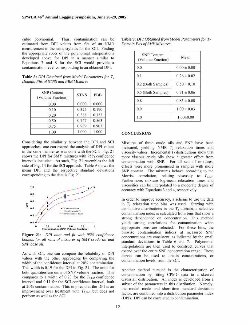
12

Considering the similarity between the DPI and SCI approaches, one can extend the analysis of DPI values in the same manner as was done with the SCI. Fig. 21 shows the DPI for SMY mixtures with 95% confidence intervals included. As such, Fig. 21 resembles the left side of Fig. 14 for the SCI approach. Table 9 shows the mean DPI and the respective standard deviations corresponding to the data is Fig. 21.

0.0

0.2

0.4

0.6

0.8

1.0


DPI

Experimental DataCubic Polynomial Fit95% Confidence Bound

Figure 21: DPI data and fit with 95% confidence bounds for all runs of mixtures of SMY crude oil and SNP base oil. As with SCI, one can compare the reliability of DPI values with the other approaches by comparing the width of the confidence interval at 20% contamination. This width is 0.19 for the DPI in Fig. 21. The units for both quantities are units of SNP volume fraction. This compares to a width of 0.23 for the T2,LM confidence interval and 0.11 for the SCI confidence interval, both at 20% contamination. This implies that the DPI is an improvement over treatment with T2,LM, but does not perform as well as the SCI.

Table 9: DPI Obtained from Model Parameters for T2 Domain Fits of SMY Mixtures

SNP Content (Volume Fraction) Mean

0.0 0.00 ± 0.00

0.1 0.26 ± 0.02

0.2 (Both Samples) 0.50 ± 0.10

0.5 (Both Samples) 0.71 ± 0.06

0.8 0.85 ± 0.00

0.9 1.00 ± 0.03

1.0 1.00±0.00 CONCLUSIONS Mixtures of three crude oils and SNP have been measured, yielding NMR T2 relaxation times and viscosity values. Incremental T2 distributions show that more viscous crude oils show a greater effect from contamination with SNP. For all sets of mixtures, effects were more pronounced in samples with more SNP content. The mixtures behave according to the Morriss correlation, relating viscosity to T2,LM. Furthermore, mixture log-mean relaxation times and viscosities can be interpolated to a moderate degree of accuracy with Equations 3 and 4, respectively. In order to improve accuracy, a scheme to use the data in T2 relaxation time bins was used. Starting with cumulative distributions in the T2 domain, a selective contamination index is calculated from bins that show a strong dependence on concentration. This method yields strong correlations for contamination when appropriate bins are selected. For these bins, the binwise contamination indices at measured SNP concentrations are consistent, as indicated by the small standard deviations in Table 6 and 7. Polynomial interpolations are then used to construct curves that extend over the entire SNP concentration range. These curves can be used to obtain concentrations, or contamination levels, from the SCI. Another method pursued is the characterization of contamination by fitting CPMG data to a skewed Gaussian distribution. An index is developed from a subset of the parameters in this distribution. Namely, the model mode and short-time standard deviation factor, are combined into a distribution parameter index (DPI). DPI can be correlated to contamination.


13

Comparing the two methods above, the DPI is less reliable than the SCI in terms of the uncertainty in degree of contamination corresponding to a particular index value. However, it does outperform the T2,LM method using the same criteria. Thus, using the SCI or DPI approaches would be recommended improvements to characterizing contamination using T2,LM. ACKNOWLEDGEMENTS The authors would like to acknowledge the Consortium on Processes in Porous Media at Rice University and the US DOE Grant DE-PS26-04NT15515 for financial support. In addition, Dr. Robert Freedman of Schlumberger was instrumental in motivating the measurements mentioned. References Cited Akkurt, R., Fransson, C.-M., Witkowsky, J.M.,

Langley, W.M., Sun, B., and McCarty, A. 2004. “Fluid Sampling and Interpretation with the Downhole NMR Fluid Analyzer.” Paper 90971 presented at the 2004 SPE ATCE. Houston, TX.

Bouton J., Prammer M. G., Masak P., and Menger S. 2001. “Assessment of Sample Contamination by Downhole NMR Fluid Analysis.” Paper 71714 presented at 2001 SPE ATCE. New Orleans, LA.

Chen, S., Zhang, G, Kwak, H., Edwards, C.M., Ren, J., and Chen, J. 2004. “Laboratory Investigation of NMR Crude Oils and Mud Filtrates Properties in Ambient and Reservoir Conditions”. Paper 90553 presented at 2004 SPE ATCE. Houston, TX.

Chuah, T. L. 1996. Estimation of Relaxation Time Distribution for NMR CPMG Measurements. M.S.Thesis. Rice University, Houston, TX.

Lo, S.-W. 1999. Correlations of NMR Relaxation Time with Viscosity/Temperature, Diffusion Coefficient and Gas/Oil Ratio of Methane-Hydrocarbon Mixtures Ph.D. Thesis. Rice University, Houston, TX.

Masak P. C., Bouton J., Prammer M. G., Menger S., Drack E., Sun B., Dunn K.-J., Sullivan, M. “Field Test Results and Applications of the Downhole Magnetic Resonance Fluid Analyzer,” paper GGG, presented at SPWLA 43rd Annual Logging Symposium. Oiso, Japan (2002).

Morriss, C.E., Freedman, R., Straley, C., Johnston, M., Vinegar, H.J., and Tutunjian, P.N. 1997. “Hydrocarbon Saturation and Viscosity Estimation from NMR Logging in the Belridge Diatomite.” The Log Analyst. March-April, p. 44.

ABOUT THE AUTHORS Arjun Kurup received a BChE in Chemical Engineering from the University of Minnesota, Twin Cities in 1999. Arjun is currently a Ph.D. candidate in Chemical Engineering at Rice University under the direction of Dr. George J. Hirasaki. His research interests are in NMR fluid properties with topics including drilling mud contamination of crude oils, NMR correlations for natural gas mixtures, and NMR properties of live oils. Dr. George J. Hirasaki obtained a BS from Lamar University in 1963 and a PhD from Rice University in 1967, both in Chemical Engineering. George had a 26 year career with Shell Development and Shell Oil Companies before joining the Chemical Engineering faculty at Rice University in 1993. At Rice, his research areas are in NMR well logging, reservoir wettability, enhanced oil recovery, gas hydrate recovery, asphaltene deposition, emulsion coalescence, and surfactant/foam aquifer remediation.

effect of drilling-mud base-oil contamination on crude...

Documents