effect of compressive force on aeroelastic stability of a ... · pdf filefor the wing flutter...
TRANSCRIPT

Effect of Compressive Force on AeroelasticStability of a Strut-Braced Wing
Erwin Sulaeman
Dissertation submitted to the Faculty of theVirginia Polytechnic Institute and State University
in partial fulfillment of the requirements for the degree of
Doctor of Philosophyin
Aerospace Engineering
Rakesh K. Kapania, ChairBernard Grossman
Eric R. JohnsonLiviu Libresu
William H. MasonJoseph A. Schetz
November 26, 2001Blacksburg, Virginia
Keywords: Aeroelasticity, Strut-Braced Wing, Unsteady Aerodynamics,Non-uniform Beam Finite Element, Buckling
Copyright ©2001, Erwin Sulaeman

Effect of Compressive Force on Aeroelastic Stability
of a Strut-Braced Wing
by
Erwin Sulaeman
Committee Chairman: Rakesh K. Kapania
Aerospace Engineering
(ABSTRACT)
Recent investigations of a strut-braced wing (SBW) aircraft show that, at high
positive load factors, a large tensile force in the strut leads to a considerable compressive
axial force in the inner wing, resulting in a reduced bending stiffness and even buckling of
the wing. Studying the influence of this compressive force on the structural response of
SBW is thus of paramount importance in the early stage of SBW design.
The purpose of the this research is to investigate the effect of compressive force on
aeroelastic stability of the SBW using efficient structural finite element and aerodynamic
lifting surface methods. A procedure is developed to generate wing stiffness distribution for
detailed and simplified wing models and to include the compressive force effect in the SBW
aeroelastic analysis. A sensitivity study is performed to generate response surface equations
for the wing flutter speed as functions of several design variables. These aeroelastic
procedures and response surface equations provide a valuable tool and trend data to study the
unconventional nature of SBW.
In order to estimate the effect of the compressive force, the inner part of the wing
structure is modeled as a beam-column. A structural finite element method is developed
based on an analytical stiffness matrix formulation of a non-uniform beam element with

iii
arbitrary polynomial variations in the cross section. By using this formulation, the number of
elements to model the wing structure can be reduced without degrading the accuracy.
The unsteady aerodynamic prediction is based on a discrete element lifting surface
method. The present formulation improves the accuracy of existing lifting surface methods
by implementing a more rigorous treatment on the aerodynamic kernel integration. The
singularity of the kernel function is isolated by implementing an exact expansion series to
solve an incomplete cylindrical function problem. A hybrid doublet lattice/doublet point
scheme is devised to reduce the computational time.
SBW aircraft selected for the present study is the fuselage-mounted engine
configuration. The results indicate that the detrimental effect of the compressive force to the
wing buckling and flutter speed is significant if the wing-strut junction is placed near the
wing tip.

iv
Dedication
This work is dedicated to the memories of
my mother, Amanah
and my father, Ma’mun

v
Acknowledgement
I would like to express my sincere gratitude and appreciation to the chairman of my
committee, Prof. Rakesh Kapania, for his guidance and advice during the course of this
research. I am grateful for his support and giving me the opportunity to involve in many
important projects: the truss-braced wing, UCAV and ZONA aeroelastic projects. His
encouragement, thoughtfulness, and supervision are deeply acknowledge. He will always be
my guru.
I would like to thank Profs. Bernard Grossman, William Mason, and Joseph Schetz for
their valuable guidance, constructive ideas, and generosity in sharing their experiences. I
have been very fortunate to receive invaluable lessons especially during the weekly meeting
of the truss-braced wing project. I am very grateful to Prof. Eric Johnson for his important
advice. I learned a lot on wing structure models from his thin-wall structure class notes. I
would like to thank Prof. Liviu Librescu who introduced me the beauty of aeroelasticity in
his excellent lectures. I must also express my gratitude to Prof. Raphael Haftka of University
of Florida for his useful guidance. I wish to acknowledge my sincere thanks to Profs. Daniel
Inman and Harry Robertshaw of CIMMS, Virginia Tech, who provided me with a valuable
opportunity when I worked for a short duration on the UCAV project. I owe a lot to Prof.
Danny Liu of Arizona State University and P.C. Chen of ZONA Tech for their valuable
support and assistance. ZONA Tech has been very kind to let me use their facilities during
the final stage of the present work.

vi
I would like to thank my friends in TBW and UCAV projects, especially to Amir,
Anand, Andy, Frank, Jay, Joel, and Philippe for their support and encouragement. I would
like to thank Goyal, Iridiastadi and Rildova for their readiness when I needed their help.
I would like to acknowledge that the financial support received during the first three
years of my graduate study was provided from the science and technology for industrial
development (STAID) project of the Indonesian Agency for the Assessment and Application
of Technology. The truss-braced wing project was sponsored by NASA Langley Research
Center, Grant No. NAG1-1852.
Finally, I would like to express my deep appreciation to my beloved wife, Dwityastuti,
for her unconditional help, sacrifice and patience. I am forever grateful to my family for their
love.

vii
Contents
Abstract ii
Dedications iv
Acknowledgements v
List of Figures xii
List of Tables xvi
List of Symbols xviii
1 Introduction 1
1.1 Literature Review 3
1.1.1 Strut-Braced Wing Aircraft 3
1.1.2 Structural Wing Modeling 5
1.1.3 Non-Uniform Beam Finite Element Formulation 8
1.1.4 Unsteady Aerodynamic Load Formulation 11
1.1.5 Strut-Braced Wing Aeroelasticity 21
1.2 Dissertation Outline 23
1.3 Contribution to the Field 24

viii
2 Strut Braced Wing Aeroelasticity Without Geometric Stiffness Effect 26
2.1 Introduction 26
2.2 Wing Cross Section Model 32
2.2.1 Double Plate Model 32
2.2.2 Basic Hexagonal Wing Section Model 34
2.2.3 Equivalent Hexagonal Wing Section Model 36
2.3 Finite Element Model 41
2.4 Flutter Analysis Using NASTRAN 43
2.5 Sensitivity Analysis 52
3 Nonuniform Beam Element Formulation 61
3.1 Introduction 61
3.2 Axial Stiffness Matrix of Non-uniform Beam Elements 64
3.2.1 Deformation of the Cantilever Beam Problem 65
3.2.2 Flexibility Matrix 67
3.2.3 Stiffness Matrix 68
3.3 Torsional Stiffness Matrix of Non-uniform Beam Elements 68
3.4 Flexural Stiffness Matrix of Non-uniform Beam Elements 69
3.4.1 Displacement of a Cantilever Beam Problem 70
3.4.2 Flexibilty Matrix of the Cantilever Beam 74
3.4.3 Stiffness Matrix 74
3.5 Non-uniform Load 75
3.6 Non-symmetric Beam Cross Section 78
3.7 Geometric Stiffness Matrix Formulation 80
3.8 Validation 84
3.9 Buckling Analysis of the Strut-Braced Wing 88

ix
4 Aerodynamic Load Formulation 92
4.1 Introduction 92
4.2 Theoretical Background 93
4.2.1 Assumptions 93
4.2.2 Basic Concept 93
4.2.3 Boundary Conditions 98
4.2.4 Evaluation of the Kernel Function 98
4.2.5 Evaluation of the Aerodynamic Operator 101
4.2.6 Discrete Element Lifting Surface Methods 103
4.2.7 Doublet Lattice Method of Rodden et al 104
4.2.8 Doublet Point Method of Ueda and Dowell 110
4.2.9 Doublet Hybrid Method of Eversman and Pitt 115
4.3 Contribution of the Present Work 115
4.3.1 The Doublet Lattice Method (DLM) 116
4.3.2 The Doublet Point Method (DPM) 117
4.3.3 The Doublet Hybrid Method (DHM) 117
4.4 Alternate Expansion Series for the Incomplete Cylindrical Function 120
4.5 Present Vortex Lattice Method 123
4.6 Present Doublet Point Method 127
4.6.1 Present DPM for Planar Lifting Surfaces 127
4.6.2 Present DPM for Non-planar Lifting Surfaces 130
4.7 Present Doublet Lattice Method 136
4.7.1 Present DLM for Planar Lifting Surfaces 137
4.7.2 Present DLM for Non-planar Lifting Surfaces 139
4.8 Present Doublet Hybrid Method 141
4.9 Unsteady Aerodynamic Load in Laplace Domain 144
4.8.1 Kernel Function Formulation 145

x
4.8.2 Incomplete Cylindrical Function 147
4.8.3 Application to the Strut-Based Wing Aeroelastic Analysis 149
4.10 Validation 150
4.9.1 Delta Wing with AR = 2 151
4.9.2 Double-Delta Wing 153
4.9.3 Sweptback Wing with Partial Flap 154
4.9.4 AGARD Wing—Horizontal Tail 156
4.9.5 Strut-Based Wing with Camber and Twist Angle 158
4.11 Unsteady Transonic Aerodynamic 161
5 Strut Braced Wing Aeroelasticity With Geometric Stiffness Effect 167
5.1 Introduction 167
5.2 The Flutter K-Method 169
5.2.1 Theoretical Background 169
5.2.2 Validation of the Present Flutter Procedure 173
5.3 The Compressive Force Effect 176
5.4 Trim Analysis of the Strut-Braced Wing 178
5.5 Modal Analysis 182
5.6 Flutter Calculation at Reference Condition 186
5.7 Sensitivity Analysis 190
6 Conclusion 195
7 Further Work 198
References 200
Appendices

xi
A Detailed Derivation of the Kernel Function Integration A.1
B Sample Input and Output B.1
C Minimum Denominator Rational Function C.1
D Translation of Axis Procedure D.1
Vita V.1

xii
List of Figures
1.1 The strut-braced wing aircraft with fuselage-mounted engine configuration. 2
1.2 The rectangular wing box models for the joined-wing structure model. 6
1.3 The double-plate and the hexagonal box models for the strut-braced wing
structure model. 7
1.4 The strut-braced wing model of the Keldysh problem. 22
1.5 The present aeroelastic computational module of the strut-braced wing. 25
2.1 The SBW model of the Keldysh problem. 28
2.2 A space frame model of the present strut-braced wing. 30
2.3 Front view of the present strut-braced wing. 30
2.4 The double plate model to represent the wing bending box. 32
2.5 The hexagonal wing section model. 35
2.6 EIxx distribution (G lb ft2) of the double plate model and three hexagonal
models based on the procedures 1, 2, and 3. 38
2.7 (a) The double plate model, (b) The equivalent hexagonal model 1,
(c) The equivalent hexagonal model 2. 39
2.8 The strut braced wing frame generated using ehexa.f. 43
2.9a Mode1: First vertical bending( 2.33 Hz). 44
2.9b Mode 2: Second vertical bending ( 2.97 Hz). 45
2.9c Mode3: Third vertical bending( 3.74 Hz). 45

xiii
2.9d Mode 4: First aft bending ( 4.37 Hz). 46
2.9e Mode 5: Fourth vertical bending ( 6.76 Hz). 46
2.9f Mode 6: Second aft bending ( 7.71 Hz). 47
2.9g Mode 7: First Torsion ( 9.09 Hz). 47
2.10 The flutter V-g and V-f plots. 50
2.11 The V-g plot of the strut braced wing at the reference condition. 51
2.12 Flutter speed as a function of the strut junction position at the fuselage in
the x (longitudinal) direction. Vref = 902 fps. 54
2.13 Flutter speed as a function of the spanwise position of the strut junction at
the wing. Vref = 902 fps. 55
2.14 Flutter speed as a function of the chordwise and spanwise position of
the wing-strut junction. Vref = 902 fps. 57
2.15 Flutter speed, at sea level, as a function of the length of the offset beam
connecting the wing and strut. Vref = 902 fps, hoffset-Ref = 3.17 ft. 58
2.16 Flutter speed, at sea level, as a function of the length of the offset beam
connecting the wing and strut. Vref = 902 fps, hoffset-Ref = 3.17 ft. 60
3.1 Geometry and sign convention of a tapered axial bar element. 61
3.2 A cantilever beam model to derive the flexibility matrix. 64
3.3 Geometry and sign convention of a tapered beam element. 66
3.4 A cantilever beam model to derive the flexibility matrix. 71
3.5 A non-uniform beam element under a non-uniform distributed load. 77
3.6 Convergence of the error of the tip displacement of the cantilever non-
prismatic beam under a concentrated moment load M at the tip.
86
3.7 A space frame geometry consisted of uniform and tapered beam elements. 85

xiv
3.8 Convergence of the displacement of Point 1 of the space frame structure. 87
3.9 A non-prismatic beam with several supports. 88
3.10 A space frame model of the wing-strut configuration. 89
3.11 Buckling load versus spanwise location of the strut junction. 90
3.12 Buckling load versus the offset beam length and stiffness. 91
4.1 The induced velocity at point P (x,y,z) due to pressure loading on
an infinitesimal area dξ dη concentrated at point (ξ, η, ζ). 95
4.2 Lifting surface idealization in the doublet lattice method. 104
4.3 The lifting surface idealization in the doublet point method. 111
4.4 Lifting surface idealization in the vortex lattice method. 124
4.5 Vortex segment geometry. 125
4.6 Lifting surface discritezation in the present doublet lattice method. 136
4.7 Spanwise lift distribution of a delta wing with AR=2 and M=0.13. 152
4.8 A double delta wing planform with AR=1.7. 153
4.9 A sweptback wing with partial flap. 155
4.10 Pressure distribution at y = 1.95 of the swept-back wing with flap. 155
4.11a Schematic of AGARD coplanar wing-horizontal tail configuration. 156
4.11b The lift curve slope CLα of AGARD wing-horizontal tail as a function of
the vertical gap between the wing and horizontal tail.
157
4.12 Strut-braced wing camber and twist angle for y < 0.4. 159
4.13 Lift distribution of the strut-braced wing with camber and twist angle
distribution. 160
4.14 Typical transonic dip plots near the sonic Mach number. 162

xv
5.1 The AGARD Standard 445.6 wing planform. 175
5.2 The V-g plot of the AGARD 445.6 wing at M = 0.90. 175
5.3 The V-f plot of the AGARD 445.6 wing at M = 0.90. 176
5.4 Flowchart for the flutter analysis of the strut braced wing. 178
5.5 A bilinear stress-strain relationship of the strut for calculation of wing
response under aerodynamic loading. 181
5.6 Flow chart for the trim analysis of the SBW wing under aerodynamic loads 182
5.7a Mode 1 ( 2.23 Hz). 183
5.7b Mode 2 ( 3.07 Hz). 184
5.7c Mode 3 ( 3.72 Hz). 184
5.7d Mode 4 ( 4.78 Hz). 185
5.7e Mode 5 ( 6.65 Hz). 185
5.7f Mode 6 ( 8.54 Hz). 185
5.7g Mode 7 ( 9.17 Hz). 186
5.8 The V-g and V-f plots of the strut braced wing at the reference condition. 189
5.9 Flutter speed as a function of the spanwise position of the strut junction at
the wing. Vref = 834.6 fps. 191
5.10 Flutter speed as function of the length of the offset beam at wing strut
junction. Vref = 834.6 fps.
192
5.11 Flutter speed boundary of the strut braced wing. Vref = 834.6 fps. 194

xvi
List of Tables
1.1 Non-uniform beam stiffness and load functions. 10
1.2 Unsteady planar lifting surface formulation. 12
1.3 Kernel function formulation for unsteady lifting surface aerodynamics. 13
1.4 Solution to the incomplete cylindrical function occurring in the kernel
function of the unsteady lifting surface theory. 15
2.1 Strut-braced wing aircraft parameters. 31
2.2 Natural frequencies of the strut-braced wing. 44
4.1 The coefficients aI in Laschka approximation series. 107
4.2 The number of Gauss integration points N. 138
4.3 List of procedures used in the doublet hybrid method. 142
4.4 Lift coefficient CL of a delta wing with AR=2 and α= 4.3°. 154
4.5 The lift coefficient of a double delta wing with AR=1.7 and α=1°. 153
4.6 The lift coefficient CL of the wing with partial flap. AR=2.94, α = 0°,
δ = 0.66°, k = 0.372. 154
4.7 The lift coefficient CLH / ik of AGARD wing-horizontal tail harmonically
plunging with k= 1.5 and M = 0.8. 156
5.1 Comparison of flutter speed and frequency of the AGARD 445.6 flexible
wing. 174

xvii
5.2 Strut-braced wing aircraft parameters. 162
5.3 Natural frequencies of the strut-braced wing. 169
5.4 Comparison of the flutter speed and frequency of the strut braced wing. 174

xviii
List of Symbols
A Cross-section area of a beam element
AR Aspect ratio of a lifting surface
b Semichord length of a root chord, or reference length
Bn The incomplete cylindrical function
c Chord length
CL Complex lift coefficient
CLa Complex lift-curve slope
Cm Complex moment coefficient
Cn Complex normal force coefficient
CNa Complex normal-curve slope
E Modulus of elasticity
e Element/panel semiwidth
fij Flexibility matrix coefficient
G Shear modulus
g Structural damping, also flight load factor
h Vertical displacement amplitude of a lifting surface
I Moment of inertia
In2/ rBn
In The modified Bessel function of the first kind and order n
ℑ Aerodynamic operator

xix
J Torsional constant
K Kernel function, also stiffness matrix
K1 The planar part of the kernel function*1K 2
1 / rK
K2 The nonplanar part of the kernel*2K 4
2 / rK
K10 Planar part of the kernel function for steady case
K20 Nonplanar part of the kernel function for steady case
Kg Geometric stiffness matrix
Kn The modified Bessel function of the second kind and order n
k Non-dimensional reduced frequency
L Lift force, also length of beam element
Ln The modified Struve function of the order n
M Mach number, also bending moment
P Axial force
q Dynamic pressure
R 2220 rx β+
r 20
20 zy +
ra22 zy +
rb 22 zy ˆ+
rm22 ˆˆ zy +
S Total area of a lifting surface
sij Stiffness matrix coefficient
t Wing skin thickness, also time
∞U Uniform flow velocity

xx
Un The n term of the Ueda’s series defined in Equation (3.27)
u, v, w The backwash, sidewash and downwash velocities
u1 rX /−
V Lateral force
v Lateral displacement
Wn The weighting function in the Gaussian quadrature formula.
X ( ) 20 /β− RMx
X122 rX +
x, y, z Global coordinates of a receiving point
zyx ˆ,ˆ,ˆ Local coordinates of a receiving point defined in Equation (3.27)
x0, y0, z0 ( ) ( ) ( )ζ−η−ξ− zyx ,,
mmm zyx ,, ( ) ( ) ( )ζ−η−ξ− ˆˆ,ˆˆ,ˆˆ zyx
ya, yb eyey +− ˆ,ˆ
Γ Gamma Function
α Angle of attack
β 21 M−
γ Euler’s constant = 0.577215664901532860606512…
sr γγ , Dihedral angles of receiving and sending elements respectively
γ sr γ−γ
ζηξ ,, Global coordinates of a sending point
ccc ζηξ ,, Global coordinates of the doublet point of sending element
ζηξ ˆ,ˆ,ˆ Local coordinates of a sending point defined in Equation (3.27b)
ω Frequency
∞ρ Uniform flow density

xxi
Λ Sweep angle of a quarter chord line of each element
ϕ Velocity potential
ρ Air density
∇ The Lagrange operator
Subscripts and Superscripts
c The distance form the doublet point, also spar caps
h Heaving motion
i Imaginary part
L, l Lift force
m The distance from the middle of a doublet lifting line
N, n Normal force
r Real parts
reg Regular or non-singular functions
sing Singular functions
s Sending point, also stringer
x In a chordwise or x direction
y In a spanwise or y direction
0 The distance from the middle of a doublet lifting line in a global coordinates
1 Planar parts, also the first term of a series
2 Nonplanar parts, also the second term of a series
- Amplitude of a sinusoidal motion
^ The position based on a local coordinate of each element

xxii
Abbreviations
AIAA American Institute of Aeronautics and Astronautics
AGARD Advisory Group for Aerospace Research and Development
CIMMS Center for Intelligent Material Systems and Structures (CIMSS)
FAA Federal Aviation Administration
FAR Federal Aviation Regulation
MDO Multidisciplinary Design Optimization
MAD Center Multidisciplinary Analysis and Design Center
NACA National Advisory Committee for Aeronautics
NASA National Aeronautics and Space Administration
SBW Strut-Braced Wing
UCAV Unmanned Combat Air Vehicle

Chapter 1
Introduction
For the last half-century, the design of large transonic transport aircraft throughout the
world is dominated by a cantilever wing configuration. Many improvements have been made
to increase the aircraft performance, but very few diverted from the cantilever wing based
design. It is unlikely that a big jump in performance will be possible without a significant
departure in vehicle configuration.
In recent years, however, numerous aircraft configuration concepts have been
introduced to find a better alternative to the conventional cantilever wing design. A strut-
braced wing (SBW) aircraft, Fig. 1, is one such candidate that has the potential for both a
higher aerodynamic efficiency and a lower structural weight than a cantilever wing aircraft.
Recent research suggests that the major contribution to the improvement of the strut braced
wing is due to favorable interactions between structures, aerodynamics and propulsion 1-7 and
the use of Multidisciplinary Design Optimization (MDO) to fully exploit the most desirable
synergism among these fields8-22.
Due to the unconventional nature of the strut-braced wing, specific researches on
different fields related to its design have been conducted. An important innovation in the
form of a telescoping sleeve mechanism for the strut has been proposed by the
Multidisciplinary Analysis and Design Center (MAD) of Virginia Tech to prevent strut
buckling in a negative-g load maneuver8-10. Investigation of the wing-strut interference drag

2
has been conducted in Refs. 11 and 12. Comprehensive study of the MDO aspects of the
strut braced wing were presented in Refs. 8-10 and 17-21.
In the present work, the aeroelastic aspect of the strut braced wing was investigated,
and an in-house code, to perform the aeroelastic analysis in an MDO environment, was
developed. The code takes into account the influence of the compressive force effect on the
aeroelastic analysis. Structural and aerodynamic aspects of the aeroelasticity, including wing
modeling, non-uniform beam formulation, unsteady lifting surface aerodynamic formulation
and flutter solution, are incorporated in the code.
In the present chapter, a review of the literatures related to the present work will be
presented first, including a survey on strut braced wing research, wing modeling, non-
uniform finite element beam formulation, unsteady aerodynamics, and wing aeroelasticity.
The last section of this chapter presents the contribution of the present work to the field.
Figure 1.1. The strut-braced wing aircraft with fuselage-mounted engine configuration

3
1.1 Literature Review
1.1.1 Strut Braced Wing Aircraft
A strut-braced wing (SBW) aircraft is a transport aircraft configuration with a strut
connected between the wing and the fuselage, as shown in Fig. 1. The strut-braced wing
configuration, actually, have been used both in the early days of aviation and is being used in
today’s small airplane. In the early days, the strut was needed to give additional support to
the wing with thin airfoil section or to the double wing. However, the presence of the strut,
without a proper strut shape design and arrangement, resulted in a significant drag penalty.
On the other hand, improvement on a cantilever wing structure, with appropriate wing-box
reinforcement and advancement of composite material, makes it less attractive to use the
external strut to support the wing of a large transport aircraft21.
However, the idea of the strut-braced wing has continued in the aerospace research
and industry. In 1954 Pfenninger of Northorp1 introduced the SBW concept as a means to
reduce the induced drag through an increase of the wing aspect ratio for a long range
transport. In the 1960s, Lockheed investigated the use of the strut-braced wing on a C-5A
fuselage for a long range military transport2. In 1978, Kulfan and Vachal3 of Boeing showed
the advantage of the SBW performance over a cantilever wing in a preliminary design study
of a large subsonic military plane. Turriziani et al.5 addressed fuel efficiency advantage of
the SBW of aspect ratio 25. Gradually, through these efforts, it was understood that the
bending moment of the wing can be reduced by employing the strut appropriately. Therefore
it becomes possible to reduce wing weight, to reduce airfoil thickness or to increase the wing
aspect ratio. The increase of wing span may decrease the induced drag. Also, a lower wing
thickness allows a reduction in transonic wave drag and, hence, allows a reduction in wing
sweep angle. Reduced wing swept angle and increased wing aspect ratio provide a
possibility for a region of laminar flow, and hence less skin friction drag on the wing’s

4
surface. The reduction in the weight and an enhanced aerodynamic efficiency results in both
a smaller engine and less fuel consumption.
Consequently, because of the tight coupling between aerodynamics, structures and
propulsion, an MDO approach is needed to fully exploit the synergism of these fields.
Previous implementations of the MDO approach in aircraft design, showed that the overall
performance can be improved significantly.14-16 In 1996, Dennis Bushnell, chief scientist of
NASA Langley Research Center, challenged the Multidisciplinary Analysis and Design
(MAD) Center of Virginia Tech to apply MDO methodology to the design of the strut-braced
wing aircraft concept7,8. The strut braced wing was designed to have a range of 7,500
nautical miles, 325 passengers, and a cruise Mach number of 0.85. Three configurations
were investigated including the SBW configurations with under-wing engine, wing-tip
mounted engine and fuselage-mounted engine 9-12. The multidisciplinary teams of graduate
students and faculty members worked on aerodynamics, structure and the integration of the
fields in an MDO framework. Contributions of the Virginia Tech team to the SBW design
have been published in Refs. 7 – 12, and 16 - 22.
Earlier studies on a strut-braced wing have shown that, without any special treatment,
the strut may exhibit a large deformation or even buckle under a negative-g load maneuver.
Park in Ref. 4 reported that, a significant increase in the strut size was needed to avoid the
strut buckling. To answer this major design issue, the Virginia Tech team proposed an
important contribution: a telescoping sleeve mechanism for the strut that permits the strut to
be inactive during a negative-g flight maneuver7,9. For a typical single strut design this
means that the strut would first engage in tension at some positive load factor. This can be
achieved by providing a slack in the wing strut mechanism. To prevent the strut from
engaging and disengaging during cruise due to wind gust loads, the strut was designed to
initially engage at the load factor of 0.8 g.
Another major challenge in the SBW design is the interference drag between the
wing, strut and fuselage. To address the problem, a computationally intense investigation has
been conducted using CFD tools to predict the interference drag of a streamlined strut

5
intersecting a surface in transonic flow11,12. The investigation is for a generic case employed
to simulate the flowfield in the vicinity of wing-strut, wing-pylon, and wing-body junctions.
Several parameters influencing the interference drag are investigated including the strut-wall
angle, strut thickness to chord ratio and cruise Reynolds number. By constructing a response
surface function of the interference drag with respect to these parameters, the MDO module
of the strut braced wing can exploit the influence of the interference drag to the global
design.
A detailed investigation of the effect of the MDO design constraints on the three
different SBW configurations and one cantilever wing aircraft has been performed in Refs.
17 and 18. The three SBW aircraft investigated include the fuselage-mounted engine, the
under-wing engine, and wing-tip mounted engine configurations. The study revealed that in
all the design configurations, the aircraft range is the most crucial constraint in the design.
The results showed also that all three SBW design were less sensitive to constraints than the
cantilever wing aircraft.
1.1.2 Structural Wing Modeling
For a conventional cantilever wing aircraft, a common approach to estimate the
aircraft weight is by using the weight estimation routine from NASA Langley’s Flight
Optimization System (FLOPS)23. For unconventional aircraft designs, however, some
modifications to the FLOPS routine are needed to include the influence of the unique
characteristics of such designs. For a structural investigation of the so-called joined-wing
aircraft, Kroo et al.24 proposed to use two rectangular box models for their wing structure as
shown in Figs. 1.2.a and b. Initially, their wing model used a symmetrical box with caps and
webs of uniform thickness (Fig. 1.2a). However, another study 24, 25 on the joined wing
design indicated that the most desirable arrangement for the joined-wing spars is asymmetric,
with most of the material stiffness concentrated in opposite corners of the rectangular box as
shown in Fig 1.2b. The total design variables of their latest wing box model are four,
including the cross-sectional areas of the stringers (where diagonally opposite stringers have

6
the same area) for the bending weight, and the web and skin thickness for the shear and
torsional weight prediction.
In the strut-braced wing design investigated in MAD Center of Virginia Tech, the
bending weight of the structural wing box was calculated initially based on the so-called
double plate model as shown in Fig. 1.3a9, 12. This model is made of upper and lower skin
panels to carry the wing bending moment The design variable needed for each wing box
section is only one since the upper and lower plate thicknesses are identical. Because of the
simplicity of the model, the double plate formulation offers the possibility to extract the wing
bending weight distribution by a closed form solution. The accuracy of the model to a
cantilever wing design has been demonstrated in Ref. 12.
-0.04-0.03-0.02-0.01
00.010.020.030.04
0 0.5 1
z/c
(a)
-0.04-0.03-0.02-0.01
00.010.020.030.04
0 0.5 1
z/c
(b)
Figure 1.2. The rectangular wing box models for the joined-wing structure model
The drawback of the double plate approach is its inability to predict the wing-box
torsional stiffness. This torsional stiffness becomes essential for calculating wing twist and
flexible wing spanload, as well as for predicting flutter speed. Therefore, in the present
work, a hexagonal wing-box model (Figure 1.3b) was proposed. The basic form of the model
was provided by Lockheed Martin Aeronautical Systems (LMAS) in Marietta, Georgia26. As
shown in Figure 1.3b, the wing section consists of four skin panels covering the upper and
lower part of the airfoil, two shear webs at the front and rear, four spar caps and four stringers
at the middle of each skin panels web. Therefore in each section there are 14 different

7
variables representing wing section sub component stiffness. Compared to the double plate
model that needs only one variable, the hexagonal model has more complicated geometry to
better simulate the shape of the airfoil and is consequently more difficult to find its optimum
stiffness directly.
To simplify the problem, Olliffe of LMAS26 suggested setting only one sub-
component as the independent variable and the other 13 sub-components as dependent
variables. For example, if the dimension of the lower-rear part of the skin is given, than the
other dimensions of the skins, shear webs, stringers and spar caps can be calculated directly.
Such direct calculation can be performed provided the aspect ratio between the sectional area
of each part of the element is known. In the present work, the use of the optimized aspect
ratio among wing section elements suggested by LMAS was employed in such a way that the
total bending weight of the double plate model is the same as the present hexagonal wing box
model. More detail description of the hexagonal wing box model will be presented in
Chapter 2.
-0.04-0.03-0.02-0.01
00.010.020.030.04
0 0.5 1
z/c
t
(a)
-0.04-0.03-0.02-0.01
00.010.020.030.04
0 0.5 1
z/c
(b)
Figure 1.3. The double-plate model (a) and the hexagonal box model (b) for the strut-braced
wing structure model
The present hexagonal wing box was employed to generate two wing models: the
detailed wing model and the simplified non-uniform beam model. Both wing models were

8
used to predict the strut-braced wing flutter speed. The detailed wing model consists of
various structural wing sub-components such as the wing skins, shear web, spars, and caps
modeled as plate and rod finite elements. The aeroelastic analysis of the detailed model was
performed using NASTRAN34, a commercially available finite element code. The detailed
model gives an accurate result for the aeroelastic analysis of the strut-braced wing. However,
the results are restricted to the case where the compressive force effect is not included. This
restriction is due to the fact that the current NASTRAN module does not include the
evaluation of the geometric stiffness matrix for the aeroelastic analysis. In addition, a direct
application of the detailed model for aeroelastic analysis in the MDO environment is
computationally expensive.
On the other hand, the simplified wing model offers a much faster calculation since
the number of element are reduced significantly. The simplified model consists of non-
uniform beam elements distributed along the elastic axis of the wing. Typical size of the
global stiffness matrix in the detailed model is 4000 x 4000, whereas that of the simplified
model is only 400 x 400. The accuracy of the simplified model is improved by employing an
exact formulation for the non-uniform beam element and by using a hexagonal wing box
model to calculate the flexural, torsional and extensional stiffness distribution of the
simplified beam. In addition, the effect of the compressive force can be included in the
aeroelastic analysis of the simplified beam. More detailed results of the aeroelastic analysis
for the detailed and simplified wings are presented in Chapters 2 and 5 respectively.
1.1.3 Non-uniform Beam Finite Element Formulation
Non-uniform cross-section beams, ranging from small frame components to large
bridge girder beams, are widely used as structural elements in many engineering fields. They
are used to improve the structural strength, to reduce structural weight, or to satisfy
architectural or aesthetical requirements. Important characteristic of non-uniform beam-

9
colums have been investigated since 1773 when Lagrange31,32 introduced an optimum non-
uniform shape of a column subject to an axial load. In aeroelasticity, non-uniform beam
models are often used to represent a wing33,34. NASA Langley35 investigated dynamic and
buckling characteristics of numerous non-uniform beam geometries for the construction of a
large structure platform in space, where, in this critical weight saving case, the use of non-
uniform members may prove worthwile35, 36.
A large number of investigations on the non-uniform beam can be classified into three
groups: (i) the study of the element static stiffness matrix36-46 and geometric stiffness
matrix46-50; (ii) the study of the dynamic stiffness matrices46,48,152-156; and (iii) the study of the
shape optimization of the beam-columns32,157-165.
The formulation of the static stiffness matrix for non-uniform beams has been studied
by many researchers36-46. Several different techniques have been adopted, including finite
element formulations36-43, finite difference methods47, and recurrence series methods44.
Gallagher and Lee48 and others proposed to use a variational principle to develop the
element stiffness matrix. Their development is based on a cubic displacement function,
which is the same as the formulation for a uniform beam. The formulation is simple yet it
proved to be superior to a piecewise stepped uniform element representation. This method is
adopted and extended in many finite element codes such as NASTRAN186 and ASTROS187.
Another approach to study beams using the finite element method is based on the
flexibility method. Weaver and Gere36 describe a procedure to construct the stiffness matrix
based on the flexibility method for a tapered beam with a linear variation of the bending
stiffness EI. The flexibility matrix is constructed first based on the tip deflection and rotation
of a cantilever beam. A direct integration of the Euler-Bernoulli differential equation is
performed to find the deflection or rotation for each concentrated force or moment unit load
at the tip of the beam. Karabalis and Beskos46 present the solution for beams with constant
width and linear depth variation. Banerjee and Williams36 follow the same procedure and
present the solution for a non uniform beam with a stiffness variation in the form shown in
Table 1.1.

10
Reference 36 deals with the formulation of a beam element for m = 1, 3, and 4;
corresponding to many beam sectional profiles such as circular, rectangular, triangular and
other regular geometric sections. Baker42 solves a more general form of the EI(x) function as
shown in Table 1.1.
Previous analytical solutions for the non-uniform are restricted only to symmetric
cross-sections, i.e the cross coupling moment of inertia Eyz is assumed to be zero. There are
at least three cases that can not be solved by using the previous analytical solutions:
Table 1.1 Non-uniform beam stiffness and load functions
Method Beam stiffness distribution function Load distribution
Karabalis andBeskos46
( ){ }mLxrEIxEI /1)( 0 +=EIyz = 0
N / A
Banerjee andWilliams36
( ){ }mLxrEIxEI /1)( 0 +=EIyz = 0
N / A
Baker42 ( ){ } qpmmLxrEIxEI /1)( 0 +=
EIyz = 0
iN
ii xsxp
p
∑=
=1
)(
0 < x < L (full span)
Present
( )jk
mN
jjc
N
i
ii cxEIxpxEI ∏∑
==
−==11
)(
( )jk
nM
jjyz
M
i
iiyz dxEIxqxEI ∏∑
==
−==1
01
)(
iN
ii xsxp
p
∑=
=1
)(
0 < x1 < x < x2 < L
M, Mi , m, mp, mq, mj, N, Ni, Np, nj = arbitrary integer number

11
(1) The first case is related to optimum shapes of columns, such as the one investigated in
Refs. 157 – 165, where EI(x) can be arbitrary. To accommodate the shape of such
optimum column, the polynomial function of the EI(x) should have arbitrary multiple
roots. In the present work, a more general stiffness distribution along the beam element
is shown in Table 1.1
(2) The second case is related to non-uniform loads applied to the beam. Baker42 solves the
static deflection problem of the non-uniform beam under a non-uniform distributed load.
However, the non-uniform load considered in Ref. 42 is applicable only for a full span of
the beam. For a more general case, where the load can be partially applied to the beam
span, the solution given in Ref. 42 can not be applied directly. In the present work, the
analytical solution for the general partially distributed load to the non-uniform beam was
developed in Chapter 3.
(3) The third case is related to the basic assumption adopted in the previous analytical
solution where the beam cross sections should be symmetric, i.e. the cross-coupling
moment of inertia term is zero. A treatment for a more general class of the problem, i.e.
for non-uniform beam with asymmetric cross section where the cross-coupling moment
of inertia distribution is also non-uniform, is developed in Chapter 3 of the present work.
1.1.4 Unsteady Aerodynamic Load Formulation
The Lifting Surface Equation
Accurate prediction of unsteady aerodynamics loads is an essential part of solving
aeroelasticity problems. This accurate estimation is required in aircraft design as it is related
directly to predicting maximum structural stresses, deflections, flight speed and flight
envelope among other quantities of interest. Significant research has been performed in the
past in analytical, numerical and experimental aspects of the problem in subsonic, transonic
and supersonic flows51-131. Such investigations are still going on in an effort to improve the
accuracy and efficiency of the prediction methods for more complicated aerodynamic

12
configurations ranging from two dimensional thin airfoils to full aircraft configurations. In
the present work, a numerical approach is proposed for predicting the aerodynamic load for
multiple lifting surfaces in steady and unsteady subsonic flows.
Based on a linearized potential aerodynamic equation, or the Laplace equation,
several basic theoretical procedures have been developed to evaluate aerodynamic loads on
unsteady thin wings or the so-called lifting surfaces51, 52 as shown in Table 1.2. All of the
approaches make use of the Green integral equation to form the working equation. The most
widely used version in aeroelasticity is the pressure – normal wash formulation52, 55 since one
deals directly with the pressure difference distribution and the velocity on the surface without
any evaluation in the wake region. This formulation was first proposed in 1935 by Kussner51
in the form shown in Table 1.2. His formulation however did not describe the detailed form
of the kernel function K that relates the pressure difference with the downwash velocity.
Table 1.2. Unsteady planar lifting surface formulation
Formulation The Integral Equation* References
Pressure - normal wash
equation ∫ ∆=
S
p dAKpw Kussner, Laschka,
Watkins et al., Giesing et al.
Velocity potential
formulation∫+
φφ∆=
WS
dAKw Jones, Stark, Houbolt,
Haviland, Singh, Liu et al.
Acceleration potential
formulation ∫ φ∆=ϕ
S
z dAKp Van Spiegel
Integrated acceleration
formulation∫+
φψ∆=ψ
WS
z dAK Stark
*S = surface region, W = wake region, ∆p = pressure difference, w = downwash velocity, φ = velocity potential, ϕ = acceleration potential, ψ = ∫ ϕ dx

13
Formulation of The Kernel Function
In 1955 Watkins et al.60 published the kernel function K as a function of the
oscillating frequency of the lifting surface and Mach number. This first formulation has been
widely used to calculate unsteady subsonic loads on planar wing - horizontal tail
configurations52,56. However, for nonplanar arrangements, such as wings with dihedral, non-
planar wing-tail configurations, T or V- tails and wings in ground-effect, a more general
approach should be performed. In light of this need, significant development in the
formulation of the kernel for nonplanar configurations have been contributed by Laschka65,
Yates63, Rodemich64, Landahl64, and Berman, Shyprykevich and Smedfjeld105. Table 1.3
shows a summary of this formulation. Laschka65 formulated the kernel function for non-
planar configurations in terms of the x, y and z components of the induced velocity vector.
Yates63 proposed the kernel function in a slightly different form for the non-planar
configurations. The most widely used formula is the one proposed by Landahl52, 62, 66, 70 – 87, 91
– 93 since it is less complicated than the other formulas mentioned above64. The Landahl’s
formulation is also used in the present work.
Table 1.3. Kernel function formulation for unsteady lifting surface aerodynamic
Contributor The kernel function form Publication
Watkins et al.(NACA)60 Planar configuration, Kw NACA R 1234 (1955)
Laschka(Germany)65 Non planar config. Ku, Kv and Kw
Z. Angew. Math. Mech.(1963)
Yates (NASA)63 Non planar config. Ku, Kv and Kw AIAA Journal (1966)
Landahl (MIT)52 Non planar config. K (unified) AIAA Journal (1967)
Berman et al.(Grumman)55
Non planar config. K inclined to thefree stream J. Aircraft (1970)
Lan (Univ. Kansas)88 Non planar config. K of oscillatinghorseshoe vortices NASA SP-405 (1976)

14
The Incomplete Cylindrical Function
All of the kernel functions formulation for the pressure-normalwash equation
summarized in Table 1.3 contains the so-called incomplete cylindrical function where the
integral limit of the function is ranging from a finite point x on the lifting surface to the
infinite point +∞. Before 1981, no exact mathematical solution to the incomplete cylindrical
function was available. The only available closed form solution was for a complete
cylindrical function where the integral limit of the kernel function is ranging from 0 to +∞.
The closed form solution for the complete cylindrical function is available in the form of
modified Bessel and modified Struve functions of the first and second kinds. More
description on the incomplete cylindrical function will be given in Chapter 4 and Appendix A
of the present work.
An attempt to approximate the incomplete cylindrical function has been first
conducted by Watkins et al. in Ref. 51 (1955). In their approximation, the integrand of the
kernel function is approximated by four term series in a form that is easily integrated. More
accurate approximations were presented by Laschka (1963)102 , Dat-Malfois (1970)103,
Desmarais (1982), and a more recent publication by Epstein and Bliss (1995)151. A summary
of these approximation was presented in Table 1.4.
The exact solution to the incomplete cylindrical function was first proposed by Ueda
in 1981 by using an expansion series approach78. The proof of the Ueda’s solution has been
presented by the present author in Ref. 135. Another exact solution was presented by
Bismarck-Nasr (1991)70 by using a differential equation approach resulting in the solution in
the form of modified Bessel, modified Struve, and sine integral functions. Both Ueda’s and
Bismarck-Nasr’s analytical solutions are converged to the solution of the complete
cylindrical function when the finite point on the surface x is set to 0. The only drawback of
those solutions is that the strong singularity terms are not easily evaluated since the
singularity terms are hidden in the series. A technique to separate the singular and regular

15
parts of the kernel function has been presented by the present author in Ref. 135 using a
modified Bessel function. In the present work, a different approach will be conducted to
analytically separate the singular and regular functions. The present approach uses an
expansion series to the complex exponential function embedded in the incomplete cylindrical
function. A new series in the form of regular term series without the modified Bessel function
term will be presented. This effort does not destroy the accuracy of the analytical solution
since the separation is performed analytically.
Table 1.4. Solution to the incomplete cylindrical function occurring in the kernel
function of the unsteady lifting surface theory
Method Solution
Watkins et al. (1955) Four term approximation series
Laschka (1963) 11 term approximation series
Dat and Malfois (1970) Seven term approximation series
Desmarais (1982) 12 term approximation series
Epstein and Bliss (1995) Three and Four term series
Ueda (1981) Analytical solution using an expansion series
Bismarck-Nasr (1991) Analytical solution using differential equation approach
Present Analytical solution using an expansion series and separationof the singular and regular functions
The Lifting Surface Method
After the kernel function has been well formulated, the next challenge for predicting
the unsteady aerodynamic load was the method to solve the integration of the kernel function.
This integration should be performed in a rather careful way since the kernel function
contains a strong singularity function when its argument is near zero. Vast literature on the

16
methods shows a gradual improvement on the accuracy, capability and efficiency of the
integration technique, as is pointed out in the survey papers in References 52, 55, 68, and 69.
The integration solution methods can be divided into two broad categories, the mode
function method (or the kernel function method) and the discrete element method66. The
mode function methods use an assumption that the pressure distribution may be
approximated by a series of orthogonal polynomial functions with unknown coefficients
which are determined by satisfying the flow tangency boundary conditions at a collocation
point.52,69. For wing with control surfaces or other complex configurations, a careful
treatment for pressure discontinuity is needed and therefore make this first method sensitive
to the manner of representing the additional singularities associated with such geometry.
The usual procedure for the second method is to divide the lifting surfaces into
infinitesimal trapezoidal panel elements which permit the assumption that the pressure load is
constant within one element. The integral equation of the pressure-normal wash equation is
represented in a discrete set of linear equations with the pressure load at each element as the
unknown. The linear equation is solved by imposing the flow tangency boundary condition
at each element. This approach, which is used in the present work, is more suitable for a
complicated lifting surface planform since a similar treatment to discritize the planform can
be performed.
Several variations of the discrete element method have been proposed. For the steady
subsonic flow, one of the well known discrete element methods is the vortex lattice method
(VLM), such as the method of Weissinger121, Falkner141, Campbell142, Hedman137,
Belotserkovskii140, Rubbert189, Dulmovits190, Margason and Lamar90, Lan88,100 and Mook et
al.186 For unsteady subsonic flow, these include the doublet lattice method (DLM) of Stark52,
Albano et al.70, Jordan71, and Giesing et al.62, 67, 72, Rodden et al.143-145, and van Zyl 146-148, the
doublet point method (DPM) of Houbolt73, and Ueda and Dowell66, the doublet strip method
of Ichikawa et al.74, and the hybrid doublet-lattice/doublet point (DHM) of Eversman and
Pitt75.

17
In the present work, a scheme to improve the numerical procedure of the doublet
lattice method, doublet point method and doublet hybrid method will be proposed. A brief
introduction to the existing DLM, DPM, and DHM methods is discussed and the new
approach is described in subsequent sections.
The Doublet Lattice Method
For a subsonic aeroelasticity analysis, the most widely-used version of the unsteady
aerodynamics method is the doublet lattice method of Rodden et al.80 because of its ready
applicability to complex nonplanar configurations. NASTRAN53, 80 uses the DLM version
developed in Refs. 12, 17 and 22 where a quadratic approximation (DLM-quadratic) is used
for integrating the kernel function. Despite the wide acceptance of the method, however, the
DLM-quadratic version is sensitive to the element aspect ratio and the number of chordwise
boxes per wavelength. To obtain acceptably accurate results for DLM-quadratic version,
NASTRAN User’s Manual80 suggests using the element aspect ratios less than 3 and at least
25 boxes per wavelength. Van Zyl146, 147 pointed out that the DLM-quadratic version
contains an inaccuracy in the integration of the elemental kernel function. He proposed to
improve the accuracy by using a piecewise cubic spline approximation to replace the
quadratic function in each element146 and reported improvement in the convergence rate147.
However, van Zyl’s DLM version required a considerable amount of calculation since for
each element the method would need a large number of interpolation points. Reference 146
shows that the interpolation points needed for convergence can be as many as 129 points per
element as compared to only 3 points per element needed for the DLM-quadratic version.
Recently, Rodden et al. 143-145 attempted to improve the accuracy of the DLM by
proposing a DLM-quartic version, a new scheme for the integration of the kernel function by
increasing the order of the polynomial approximation from a quadratic function to a quartic
function. The DLM-quartic version143, 144 allows the use of the element aspect ratio of up to
10, a considerable improvement compared to the maximum aspect ratio of 3 for the DLM-
quadratic. The DLM-quartic version, however, still requires a large number of chordwise

18
boxes per wavelength. Reference 144 suggested a minimum number of 50 chordwise boxes
per wavelength, which is significantly higher than that for the DLM-quadratic version. A
numerical study devoted to investigate the convergence of the DLM was conducted in Ref.
147 and concluded that the limitation of the DLM-quartic version is as a result of the
integration error introduced by the approximations to the kernel numerators.
Another limitation of the DLM-quadratic version was pointed in Ref. 72. In their
analysis, Rodden et al.72 mentioned that the near-coplanar configuration problem is not
completely solved. The procedure fails, for example, if the vertical separation between two
lifting surfacess is very small. For such a case, the DLM-quadratic version automatically sets
the vertical separation to be zero. For practical cases, it may be acceptable to assume the two
lifting surfaces to be coplanar if the vertical separation is very small. However, from
theoretical point of view, this indicates that an effort to improve and optimize the method is
still needed.
An effort to improve the accuracy of the method has been proposed by Jordan in Ref.
71. In his DLM version, an exact integration of the kernel at a quarter chord of the element
has been completed. However, this technique is limited to rectangular planar surfaces in
incompressible flow (M = 0). It should be noted that, if the Prandtl-Glauert compressibility
correction is taken into account, the mathematical form of the kernel function becomes very
complicated. An exact integration of the kernel function is still a challenge. In the present
work, only the singular part of the kernel function can be integrated analytically. The regular
part is integrated numerically using Gauss-Legendre quadrature technique.
One possible source of the inaccuracy in the previous DLM is the integration to the
improper cylindrical function occurring in the kernel function. The incomplete cylindrical
function in the DLM-quadratic version is solved using Laschka’s series to approximate the
integrand of the integral as described in Table 1.4. There are two disadvantages to this
scheme. First, the accuracy of Laschka’s series is limited to the order of three digits.
Second, the series approximates the integrand, and not the integral itself. Gazzini et al.82
showed that an approach to performing the integration by approximating the integrand may

19
not be equivalent to the approach to performing the integral itself. Therefore, it is believed
that the application of the exact solution to performing the improper integral directly, which
is conducted in the present work, will increase the accuracy of the previous works.
The kernel function in the DLM of NASTRAN contains regular and singular
functions as the values of r approaches zero and X > 0. There is no separation between these
functions in the DLM. Therefore the Mangler procedure is also applied to the regular
function, which is not a proper way to solve the problem. In the present work, the regular and
singular functions will be identified and treated separately.
The DLM uses a quadratic or a quartic approximation for the numerator of the kernel
to simplify the integration procedure. This procedure may be improved if one uses Gaussian
quadrature technique as is suggested by some authors 83-86. The Gaussian technique does not
need a fixed number of integration points. Less than three points may be used if the
sending/receiving panel pairs are distant or if the reduced frequency is low. If the reduced
frequency is high, or if the distance between sending and receiving panels is close such that
the kernel function may vary rapidly, one may use more than three integration points. The
improvements outlined above will be implemented in the present work.
The Doublet Point Method
The idea of the DPM was first proposed by Houbolt81 based on the pressure-velocity
potential concept, and independently by Ueda and Dowell66 based on the pressure-normal
wash concept. Houbolt (1969)81, however, did not give numerical results for three-
dimensional flows since a direct evaluation of the incomplete cylindrical function was not
available at that time. The exact solution of this type integral was given in 1981, and the first
version of the DPM was developed in 1982 for planar surfaces66.
There are two basic assumptions used in the original DPM66. First, the lifting
pressure is assumed to be concentrated at a single point located at the one-quarter chord
along the center line of each element. The point is called a doublet point. Similar to the
DLM, the control point is placed at the three-quarter chord along the mid-span of each panel.

20
Second, if the receiving point is located on the wake of the sending element, i.e. X > 0 and r
= 0, then the singularity problem occurs and the finite part of the Mangler integration
procedure should be used by utilizing an average value of the modified Bessel function to
treat the singularity problem.
Although the formulation is very simple, the DPM gives a reasonable accuracy for
various planar lifting surfaces66. However, for a lifting surface with a large swept angle, the
accuracy of the DPM can be less than that of the DLM. Rodden commented in Ref. 66 that
the DPM does not have the local sweep angle effect in their formulation. In the present DPM
formulation, it will be shown that the local sweep angle effect is incorporated in the
formulation based on a proper integration of the kernel function.
Improvements to the DPM proposed in the present study also include a treatment for
nonplanar configurations which is not considered in the original DPM66. The idea to separate
the singular and regular parts of the kernel functions is also applied to the nonplanar surface
formulation. It will be shown that some singular parts of the planar term will cancel the other
singular parts of the nonplanar term in the present formulation. This treatment clearly will
improve the accuracy of the nonplanar DPM.
Doublet Hybrid Method of Eversman and Pitt
An extension of the DPM for nonplanar interfering surfaces has been made by
Eversman and Pitt75 based on the nonplanar kernel function of Landahl. In their work, a
treatment for the singular term of the kernel nonplanar part was not well established. The
results have been reported to be less accurate than the DLM results. For this reason, they
concluded that the best approach is to utilize the nonplanar DPM only for sending/receiving
pairs which are distant. If the distance between sending and receiving points are close, they
suggest using the nonplanar DLM. This combined technique is the basis of their doublet
hybrid method (DHM). No further treatment for the limitation of DPM and DLM was
conducted, therefore some singularity problems associated with the DPM and DLM may be
found in their DHM.

21
In the present DHM, the singularity problem is identified and solved in each of the
present DPM and DLM procedures. The present DHM also unifies the present DLM and
DPM procedures such that the present DPM becomes a special case of the present DLM.
1.1.5 Strut-Braced Wing Aeroelasticity
Aeroelasticity is one important factor in the strut braced wing design. Aeroelasticity
takes into account the flexibility of the aircraft structure and its static or dynamic interaction
with the aerodynamic loads. Aeroelasticity may constraint the flight envelope, structural
weight and aircraft performance which are closely related to design variables of the MDO
tool used in the present strut braced wing design.
Most previous publications on the strut braced wing aeroelasticity deal with the static
aeroelastic response of the structure under a given aerodynamic loading. The main concern
has been usually to take advantage of the strut support for reducing wing bending moment.
Few publications have investigated the aeroelastic behavior, such as flutter and divergence,
of the strut braced wing. Reference 28 introduced the so-called “the Keldysh problem” to
analyze the aeroelastic stability of a simple wing model with a strut as shown in Figure 1.4.
The wing planform is rectangular, straight and has no dihedral. The wing aspect ratio of the
considered wing is high and the flow is assumed to be incompressible to allow the use of
simple strip theory for the unsteady aerodynamic calculation.
The bending and torsional stiffness along the wing span is assumed to be constant in
the Keldysh problem. The strut is a perfectly rigid rod connecting the wing-strut junction to
the fuselage-strut junction (Figure 1.4). Based on the Bubnov-Galerkin one term
approximation, Keldysh concluded that the wing is stable if the wing-strut junction location
ys is greater than 0.47 of the half span L. In a more recent article, Mailybaev and Seiranyan27
corrected the Keldysh’s solution by using a more rigorous approach and adding a divergence
related instability as the solution to the problem. One of their conclusions for the Keldysh
problem is that, for ys > 0.47 L, the wing will experience divergence, rather than be stable as
concluded by Keldysh. The divergence speed is twice the critical speed of a cantilever wing

22
of the same size but without a strut. Hence, for the Keldysh problem, the best location for the
wing-strut junction is between 47% of the half span and the wing tip.
x
y
z
ys
Figure 1.4 The strut braced wing model of the Keldysh problem
The Keldysh problem above demonstrates the importance of the location of the wing
strut junction. In the present work, a broader problem is considered. The wing is swept back
and tapered. The wing taper ratio is 0.21, the quarter chord swept angle is 29.9° and the
aspect ratio is 12.17. The unsteady aerodynamic load is predicted using the doublet lattice
lifting surface method which is better than the simple strip theory approach used in Ref. 22.
The strut stiffness in the present work is not infinite and the angle between the wing and strut
is very shallow (Fig. 1.1) which will impose a more flexible support at the wing-strut
junction point. Figure 1.1 also shows that the wing and strut are not in the same plane and
therefore the wing strut junction point moves elastically in the six degrees-of-freedom
deformations.
The aeroelastic analysis of the present strut-braced wing problem will be conducted
with two different wing models: detailed and simplified wing models. The analysis of the
detailed wing model will be performed using NASTRAN software. The analysis of the
simplified model will be performed using the aeroelastic analysis code developed in the

23
present work. The aeroelastic analysis results of the detailed and simplified wing model are
presented in Chapters 2 and 5, respectively.
1.2 Dissertation OutlineThe present work will be organized as follows:
• Chapter 2 presents the aeroelastic analysis of the detailed model of the strut-braced wing.
The calculation is performed using NASTRAN. No compressive force effect is included
in the calculation.
• Chapter 3 describes the formulation and validation of the structural stiffness of the
present non-uniform beam finite element.
• Chapter 4 describes the formulation and validation of the present unsteady lifting surface
methods.
• Chapter 5 presents the aeroelastic analysis of the simplified model of the strut braced
wing. The calculation is performed using the present code. The compressive force effect
is included in the calculation.
• Chapters 6 and 7 present the concluding remarks and recommendation for future work,
respectively.
• Appendix A describes the detailed derivation of the present kernel function integration
related to the formulation of the unsteady lifting surface methods in Chapter 4.
• Appendix B presents a brief description of the aeroelastic stability envelope.
• Appendices C and D describe detailed derivation of the rational function and translation
of axis needed for the FEM formulation of the non-uniform beam in Chapter 3.
1.3 Contribution to the FieldThe following are the original contributions contained in this dissertations:

24
1. An analytical formulation of the non-uniform beam stiffness is introduced to reduce the
number of elements used in the wing finite element model, and, hence, to reduce the
computational time.
The beam element stiffness distribution is an arbitrary polynomial function. The stiffness
distribution of the element includes the variation in the cross sectional area A, the
moment of inertia Iyy, Izz and Iyz, and the torsional stiffness J.
2. An iteration procedure to improve the buckling calculation of the beam is introduced
based on a Taylor expansion series.
The iteration scheme is qudratically convergent. The result gives the same result as the
standard buckling calculation if only a single iteration is performed and the initial
buckling load is zero.
3. A numerical scheme to unify the doublet-lattice and doublet point methods is introduced
to improve the accuracy and reduce the computational time. The present formulation is
derived based on analytical separation of the regular and singular functions embedded in
the lifting surface kernel function.
4. A strut-braced wing model is developed for static and dynamic aeroelastic stability
analysis. Two models were generated, including a detailed wing model and a simplified
beam model. The detailed wing model consists of 14 wing section sub-components such
as wing skins, spars, caps, and webs. The simplified beam model include the
compressive force effect in the aeroelastic calculation.
5. A procedure to include the compressive force effect in aeroelastic stability of the strut-
braced wing is developed. The developed code modules are as follows:
• ehexa.f : to generate the detailed wing model as well as the simplified model based on
the equivalent hexagonal wing box approach.
• fem.f : to generate the FEM stiffness, geometric stiffness and mass matrices of the
structural beam model.
• vlm.f : to generate the steady aerodynamic load.
• dhm.f : to generate the unsteady aerodynamic load.

25
• trim.f : to calculate the wing aerodynamic load, structural displacement, and structural
(compressive) forces for the wing under given flight load condition. The wing
flexibility and strut slack load factor are included in the analysis.
• Mode.f: to calculate the frequencies and mode shapes of the strut braced wing
including the compressive force effect.
The relationship between these modules are shown in Fig. 1.5.
wing.f ehexa.f fem.f
dhm . f flutter . f mode.f
EI, GJ, EAt/c
K - P Kg
f, Φ[A(k)]
Vf , ωf
trim.fvlm.f
K, Kg
[A]
Figure 1.5. The present aeroelastic computational module of the strut-braced wing

Chapter 2
Strut-Braced Wing Aeroelasticity
Without Geometric Stiffness Effect
2.1 Introduction
Aeroelasticity is one important factor in aircraft design. Aeroelasticity takes into
account the flexibility of the aircraft structure and its static or dynamic interaction with the
aerodynamic load. Aeroelasticity may provide a constraint on the flight envelope, structural
weight and aircraft performance. For the strut braced wing aircraft design, aeroelasticity has
a more significant role due to the unconventional nature of the aircraft as described in the
previous chapter. From the aeroelastic point of view, the strut-braced wing aircraft has at
least three important characteristics which make the aeroelastic behavior of a strut-braced
wing different from the conventional aircraft. First, the strut gives additional support to the
wing that changes the aerodynamic load distribution pattern on the wing. This aerodynamic
load redistribution further affects the wing weight and structural stiffness distribution.
Second, as a further result of multi-disciplinary optimization of various fields involved in the
design of the strut-braced wing aircraft, the wing thickness becomes thinner and the wing
aspect ratio becomes larger. With a more flexible structure, aeroelastic considerations
become even more important. Third, the presence of the compressive axial force in the inner

27
wing due to the strut force adds a geometric stiffness term to the aeroelastic set of equations.
This additional geometric stiffness term increases the complexity of the stability problem
since an eigen problem related to the wing buckling is added to the conventional aeroelastic
problem. In the present Chapter, the aeroelastic analysis of the strut braced wing is
performed by focusing on the first two aforementioned effects. The third effect, related to
the effect of compressive force on the strut braced wing aeroelastic response, is described in
Chapter 5.
Most previous publications on the strut braced wing aeroelasticity usually with the
static aeroelastic response of the structure under aerodynamic loading. The main concern is
usually to take advantage of the strut support for reducing the wing bending moment.
References 9 and 13 describe a simple approach to predicting the strut-braced wing weight
based on a double plate model for the wing section. The double plate model gives an
accurate prediction for the wing bending weight, however it is not suitable for predicting the
torsional stiffness of the wing. For this reason, Refs. 9 and 19 introduced an alternate
hexagonal section model of the wing that allows a more accurate prediction of both the wing
bending and torsional stiffness. A detailed description of the hexagonal section model used
in the present work is described in Section 2.2.
Few publications have investigated the aeroelastic behavior, such as flutter and
divergence, of the strut braced wing. Reference 28 introduced the so-called “the Keldysh
problem” to analyze the aeroelastic stability of a simple wing model with a strut as shown in
Figure 2.1. The wing planform is rectangular, straight and has no dihedral. The wing aspect
ratio is considerably high and the flow is assumed to be incompressible to allow a simple
strip theory for unsteady aerodynamic calculation.
The bending and torsional stiffness along the wing span is assumed to be constant in
the Keldysh problem. The strut is a perfectly rigid rod connecting the wing-strut junction to
the fuselage-strut junction (Figure 2.1). The wing strut junction point is on the wing elastic
axis. The rigid strut assumption imposes a pin-type support boundary condition at the wing-
strut junction point, i.e. the wing is continuous at the junction point, is free to rotate but is

28
restrained from transverse displacement. The Keldysh problem also ignores the geometric
stiffness effect.
Based on the Bobunov-Galerkin one term approximation, Keldysh concluded that the
wing is stable if the wing-strut junction location ys is beyond 0.47 of the half span L. In a
subsequent article, Mailybaev and Seiranyan27 improved the Keldysh’s solution by using a
more rigorous approach and adding a divergence related instability as a possible solution to
the problem. Their conclusions for the Keldysh problem are as follows:
(a) For ys > 0.47 L, the divergence instability is more critical than the flutter. It is found also
that the divergence speed is constant, i.e. the strut support does not improve the stability
performance if the junction point is moved further outboard.
(b) For ys = 0.47 L, the flutter speed becomes the same as the divergence speed.
(c) for ys < 0.47 L, the flutter instability is more critical than the divergence. The flutter
speed varies as the junction point moves inboard, but the flutter speed is less than the
speed at ys = 0.47 L.
(d) Therefore, the optimum location of the strut is located in the region ys > 0.47 L. The
minimum divergence speed is 60.3 m/s which is higher than the critical speed of a
cantilever wing, the same size but without strut, 30.3 m/s. Hence, for the Keldysh
problem, the strut increases the critical speed more than 100%.
x
y
z
ys
Figure 2.1 The strut braced wing model of the Keldysh problem

29
The Keldysh problem above demonstrates the effectiveness of the strut to increase the
critical speed and the importance of the location of the wing strut junction. In the present
work, a broader problem is considered. The wing is aft-swept and tapered. The wing taper
ratio is 0.21, the quarter chord swept angle is 29.9° and the aspect ratio is 12.17. The
unsteady aerodynamic load is predicted using the doublet lattice lifting surface method which
is better than the simple strip theory approach used in Refs. 27 and 28. The compressibility
of the aerodynamic load is taken into account by employing the Prandtl-Glauert
transformation in the unsteady aerodynamic governing equations.
The strut stiffness in the present work is not infinite and the angle between the wing
and strut is very shallow (Figures 2.2 and 2.3) which will impose a more flexible support at
the wing-strut junction point. Figure 2.2 also shows that the wing and strut are not in the
same plane and therefore the wing strut junction point moves elastically in the six degrees of
freedom deformations. The wing bending and torsional stiffness is not constant. A more
detailed data of the aircraft is given in Table 1.1.
The present strut-braced wing problem is solved using the MSC/NASTRAN finite
element code. The effect of the wing-strut junction position in spanwise and chordwise
directions is investigated, as well as the fuselage-strut junction point. The wing bending
stiffness is obtained based on the double plate model. In order to estimate the wing torsional
stiffness, a hexagonal wing section approach is used to model the structural wing box. A
more detailed description of the hexagonal wing section approach is described in Section 2.2.
The flutter and divergence of the strut-braced wing and the sensitivity of the wing-strut
junction location are described in Section 2.3 and 2.4 respectively.

30
x
y
z
P
The inner-wing
The outer-wing
The offset beam
The strut beam
Figure 2.2. A space frame model of the present strut-braced wing-strut
y
Figure 2.3. Front view of the present strut-braced wing

31
Table 2.1. Strut-braced wing aircraft parameters
Wing half-span 108.44 ft
Wing - strut junction point 74.52 ft
Wing sweep (3/4 chord) 25.98°
Strut sweep (3/4 chord) 19.01°
Strut offset length 2.74 ft
Wing root chord 32.31 ft
Wing tip chord 6.77 ft
Strut force at 1 g load 215 387 lb
Strut chord (constant) 6.62 ft
Wing root t/c 13.75%
Wing tip t/c 6.44%
Strut t/c 8.0%
Fuselage diameter 20.33 ft
Wing flap area 1411.02 ft2
Wing reference area 4237.30 ft2
Take-off gross weight 504833 lb

32
2.2 Wing Section Model
2.2.1 Double Plate Model
A common approach to estimating the preliminary bending weight of a conventional
wing is usually by using a semi-empirical equation such as the NASA Langley developed
Flight Optimization System FLOPS23. Application of this procedure to a strut braced wing,
however, may give inaccurate results due to the unconventional nature of the structure. For
this reason, several bending weight calculation procedures, by taking into account the
influence of the strut upon the structural wing design, were developed in the MAD Center of
Virginia Tech. The earliest work is based on a double plate assumption of the wing box
structure as reported in Refs. 13, 19, and 21.
-0.04
-0.03
-0.02
-0.01
0
0.01
0.02
0.03
0.04
0 0.2 0.4 0.6 0.8 1
z/c
cb
d
td
td
Figure 2.4. The double plate model to represent the wing bending box
To calculate the wing-bending weight of single strut configuration, a piecewise linear
beam model, representing the wing structure as an idealized double plate model, was used
first. This model is made up of upper and lower skin panels (Figure 2.4), which are assumed
to carry the bending moment. The double-plate model offers the possibility to extract the

33
material thickness distribution by a closed-form equation. The cross-sectional moment of
inertia of the wing box can be expressed as:
2ydycyt
yI2
bd )()()()( = (2.1)
where td(y) is the wing skin thickness, cb(y) is the wing box chord, and d(y) is the wing airfoil
thickness. Note that the upper and lower wing skin thickness are equal. To obtain the
bending material weight, the corresponding bending stress in the wing is calculated from:
)(2)()(
max yIydyM
=σ (2.2)
where σmax denotes the maximum stress, M(y) is the bending moment of the wing, and I(y)
denotes the cross-sectional moment of inertia.
If the wing is designed according to the fully-stressed criterion, the allowable stress
σall can be substituted into Eq. (2.2) for σmax. Substituting I(y) into Eq. (2.2), the wing panel
thickness can be specified as:
allbd ydyc
yMyt
σ=
)()(
)()( (2.3)
The chord length cb and the maximum airfoil thickness d along the wing span are
given from the wing geometry data for each iteration in the MDO optimization loop. The
bending moment M(y) is obtained by considering three critical loading cases including the –
2.0 g taxi bump, the 2.5 g pull-up, and the –1.0 g push-over maneuvers. The loading is
simplified by assuming a piecewise linear distribution along the wing span. In addition to
fulfilling the strength requirement in Eq. (2.3), this loading is also employed to calculate the
wing tip displacement constraint. The final panel thickness along the wing span is obtained
as a minimum thickness curve envelope that satisfies the structural strength and displacement
constraints for all of the loading maneuvers specified above.
Three of the most important features of the double plate approach are as follows:

34
• In each section of the wing box, only one independent variable, which is the panel
thickness td(y), is needed to represent the bending stiffness and weight.
• Since the model is simple, a closed form solution for the panel thickness can be obtained
based on the fully stressed design concept.
• The numerical procedure to approximate the wing bending weight, because of its simple
formulation, is very fast. Therefore the method is suitable for an MDO calculation
module.
The accuracy of the double plate method to approximate the wing bending weight has been
demonstrated in Refs. 12 and 17. A more detailed description of the method is described in
Ref. 12.
2.2.2 Basic Hexagonal Wing Section Model
Although the double plate model renders very accurate estimates for the wing bending
material weight, it is not suitable for calculation of the wing-box torsional stiffness. This
torsional stiffness becomes essential when calculating wing twist and flexible wing spanload,
as well as for the incorporation of aeroelastic constraints into the MDO optimization.
Therefore, a hexagonal wing-box model (Figure 2.5) was proposed for the wing
weight calculation module. The basic form of the model was provided by Lockheed Martin
Aeronautical Systems (LMAS) in Marietta, Georgia26. As shown in Figure 2.5, the wing
section consists of the following elements:
• Four skin panels covering the upper and lower part of the airfoil. Each panel has
different thickness. The skin thickness of each part is t1, t2, t4, and t5 respectively.
• Two shear web at the front and rear spars with the skin thickness t3 and t6 respectively.

35
-0.04
-0.03
-0.02
-0.01
0
0.01
0.02
0.03
0.04
0 0.2 0.4 0.6 0.8 1
z/c
t1
t5
t6
t2
t3
t4
Figure 2.5. The hexagonal wing section model
• Four spar caps at each tip of the shear web with the cross section area Ac1, Ac2, Ac3, and
Ac4, respectively. The numbering of the cap is started from the upper front spar cap and
rotated in clockwise direction.
• Four stringers at the middle of each skin panels web with the cross section area As1, As2,
As3, and As4, respectively. The numbering of the stringer is started from the middle of
upper front skin t1 and rotated in clockwise direction.
Therefore in each section there are 14 different variables representing wing section
sub component stiffness. Compared to the double plate model that needs only one variable,
the hexagonal model has more complicated geometry to better simulate the shape of the
airfoil and is consequently difficult to find its optimum stiffness directly.
To simplify the problem, Bob Olliffe of LMAS26 suggested setting only one sub-
component as the independent variable and the other 13 sub-components as dependent
variables. For example, if the dimension of t4 is given, than the other dimensions of the
skins, shear webs, stringers and spar caps can be calculated directly. Such direct calculation
can be performed provided the ratio between the sectional area of each part of the element is
known. In the present work, t4 is selected as the independent variable and the other 13 sub-

36
components are calculated based on an optimized ratio among hexagonal wing box elements
suggested by LMAS26. The ratio of each element is given in five spanwise wing sections.
The ratio of each elements in other wing sections is interpolated by using a cubic spline
approach.
The remaining part to be solved in the hexagonal box model is to find the independent
variable t4. For the strut braced wing, there are two approaches developed in the MAD
Center of Virginia Tech. The earliest approach is the equivalent hexagonal box model
developed by the present author mainly for the SBW aeroelastic analysis. The latest
approach was developed by Gern29 for predicting the SBW wing bending weight as well as
aeroelastic analysis. In Section 2.2.3, only the first method is described. A more detailed
description of the second method is given in Ref. 29.
2.2.3 Equivalent Hexagonal Wing Section Model
The equivalent hexagonal model was developed as the first attempt to find the wing
torsional stiffness distribution for aeroelastic analysis of the strut braced wing. The wing
torsional stiffness, as well as bending stiffness, was needed for flutter and divergence speed
calculations. At that time, the only available data was the wing bending stiffness distribution
calculated by using the double plate model. Since the double plate module, called wing.f, has
been validated and was well-established as part of the MDO code of the strut-braced wing,
the first idea was just to find an equivalent hexagonal model. The equivalent hexagonal
model (EHM) should have equal bending weight and bending stiffness with that of the
double plate model as shown in the following equations:
)()(2)( ycytAyA bddpmeq == (2.4a)
2)()()(
)(2 ydycyt
IyI bddpmeq == (2.4b)

37
To fulfill this goal, three procedures are investigated. Each procedure has different
assumption on the hexagonal bending weight.
2.2.3.1 Equivalent Hexagonal Model (EHM) Procedure 1
The first procedure is based on the assumption that the whole cross sectional area of
the hexagonal box is the same as the bending weight calculated using the double plate model,
or
)()(21 ycytA bdeq = (2.5)
where the bending weight of the EHM Procedure 1 is
∑= ρ
ρ=
14
11
i ref
iieq
AA (2.6)
Equation (2.6) shows that all of the 14 sub-components of the hexagonal model contribute to
the bending weight. The density ρref is the same as the density of the double plate model. If
the ratio of each sub-component area with respect to the area of the fourth skin is defined as
44
)(Lt
Ayr i
i = (2.7)
then the dimension of the fourth skin can be obtained as
∑=
=14
1i
i4
bd4
yrL
ycyt2yt
)(
)()()( (2.8)
The centroid of the hexagonal box is calculated as
∑
∑
∑
∑
=
=
=
= == 14
1
14
114
1
14
1 ;
iii
iiii
c
iii
iiii
c
EA
EzA
zEA
ExA
x (2.9)

38
Therefore, the moment of inertia Ixx of the hexagonal box can be calculated as
( )∑=
−+==14
1
2,1 )(
iciioxx
ref
ixxeq zzAI
EE
IIi
(2.10)
where the referenced Young modulus Eref is the same as the Young modulus of the double
plate model. The result of this approximation is compare to the double plate result as shown
in Fig. 2.6. The result indicates that Ieq1 is less than Idpm . Indeed, Ieq1 is always less than Idpm
because the moment arm of the EHM 1 is less than that of the double plate model. This short
coming led us to develop a second approach for the EHM. This approach is described in the
following section.
0.001
0.01
0.1
1
10
0 0.2 0.4 0.6 0.8 1
y/halfspan
EI (
x 1e
9 lb
sq
. ft)
EI double plate model
EI equivalent hexagonal model 1
EI equivalent hexagonal model 2
EI equivalent hexagonal model 3
Figure 2.6. EIxx distribution (G lb ft2) of the double plate model and three hexagonal modelsBased on the procedures 1,2, and 3

39
2.2.3.2 Equivalent Hexagonal Model (EHM) Procedure 2
The second approach is based on the assumption that the bending weight of the
hexagonal model does not include the skins and webs t1 until t6 (Figure 2.7). Therefore, the
bending weight of EHM 2 includes only the spars and stringers as follows:
∑∑ ∑== = ρ
ρ=
ρ
ρ+
ρ
ρ=
14
7
4
1
4
1
,,,,2
i ref
ii
i i ref
isis
ref
iciceq
AAAA (2.11)
such that the bending weight of the EHM 2 is the same as that of the double plate model, or
)()(22 ycytA bdeq = (2.12)
Note that the assumption to ignore the skin and web for the bending weight calculation is
commonly used in some references176.
d
AdpmAeq 1 = Atot Aeq 2 = Atot - Aweb - Askin
(a) (b) (c)
Figure 2.7. (a) Double plate model, (b) the equivalent hexagonal model 1,
(c) the equivalent hexagonal model 2
The thickness t4 is calculated by substituting of Eq. (2.11) into Eq. (2.12) and
applying the same aspect ratio of each sub-component to give
∑=
= 14
74
4
)(
)()(2)(
ii
bd
yrL
ycytyt (2.13)
td

40
Note that the index of summation in Eqs. (2.11) and (2.13) is started from i = 7 since the first
six indices belong to the skins and webs. After t4 is calculated, the dimensions of the
hexagonal sub components can be calculated based on Eq. (2.7). The sectional centroid is
calculated as:
∑
∑
∑
∑
=
=
=
= == 14
7
14
714
7
14
7 ;
iii
iiii
c
iii
iiii
c
EA
EzA
zEA
ExA
x (2.14)
The bending moment of inertia is calculated as
( )∑=
−+=14
7
2, )(
iciioxx
ref
ixx zzAI
EE
Ii
(2.15)
The moment of inertia Ixx calculated by Eq. (2.15) is still less than Idpm since the moment arm
is smaller. However, it is possible to increase the total moment inertia if we take into account
the skin and web contribution as follows:
( )∑=
−+=++=14
1
2,2 )(
iciioxx
ref
iwebskinxxeq zzAI
EE
IIIIi
(2.16)
Comparison between Ieq 2 and Idpm and Ieq 1 is given in Fig. 2.7. The second approach clearly
overpredicts the double plate model, or Ieq 1 < Idpm < Ieq 2.
2.2.3.3 Equivalent Hexagonal Model (EHM) Procedure 3
The third approach is based on the combination of the previous two approaches. The bending
weight of the third approach can be calculated as
dpm2eq21eq13eq AAaAaA =+= (2.17)
Since Aeq 1 = Aeq 2 = Adpm , then the coefficients a1 and a2 in Eq. (2.17) are related by

41
1aa 21 =+ (2.18)
The moment of inertia of the third approach is calculated as
dpm2eq21eq13eq IIaIaI ≈+= (2.19)
The last two equations, i.e. Eqs. (2.18) and (2.19), are sufficient to find the coefficients a1
and a2. The next step is to obtain the sub component area of the hexagonal model by
multiplying a1 and a2 to Ai calculated in Procedure 1 and 2 respectively. It should be noted
that there is no iteration needed in this procedure, and the Procedures 1 and 2 can be
calculated simultaneously. Therefore the computational time for this procedure is very small
and is still suitable as part of an MDO module.
Comparison between Ieq3 and other approaches are shown in Fig. 2.6. As expected,
the third approach gives a very close approximation to the double plate result. This approach
is used in the present work to provide the bending and torsional stiffness distribution for the
aeroelastic analysis.
2.3 Finite Element Model
To implement the equivalent hexagonal model procedures described in Section 2.2, a
FORTRAN computer code called ehexa.f was developed. The input data to ehexa.f is the
thickness distribution resulted from wing.f (the double plate model code) and the wing
geometry data including airfoil thickness. The output is the wing finite element model
automatically generated in a NASTRAN format. The finite element output is arranged such
that it can be used directly for static, structural dynamics and aeroelastic analyses of the strut
braced wing using NASTRAN.
There are two finite element models that can be generated by the ehexa.f. The first
model is a piecewise non-uniform beam element. The beam stiffness distributions in terms

42
of EIxx, EIzz, EIxz, EA, and GJ for each wing section are generated by the equivalent
hexagonal model procedure. The number of beam elements used are 62 elements connecting
63 structural grid points along the wing elastic axis. The finite element formulation for the
non uniform beam element is presented in Chapter 3. The aeroelastic analysis for the non-
uniform beam element is described in Chapter 5. Further description of the model is
presented in Chapters 3 and 5.
The second model is a detailed wing model consisting of the wing skins, webs, spars
and stringers. The model is used in Section 2.4 as an off-design aeroelastic analysis. The
two dimensional element such as skins and webs are modeled as quadrilateral QUAD4 or
triangular TRIA3 shells in a NASTRAN format. The one-dimensional elements, such as
spars and stringers, are modeled as ROD elements. Figure 2.8 shows the wing box structure
of this model. The number of QUAD4, TRIA3 and ROD elements are 862, 3 and 1112,
respectively. The number of nodes connected by these elements are 630. Assuming that
each node has six degrees-of-freedom, the total number of degrees-of-freedom is 3780.
Obviously, the model is not suitable to be used in the MDO since a structural analysis with
such a detailed model will need a large computational time. For this reason, the second
hexagonal model is used to verify the final MDO result. If the aeroelastic analysis module is
required as part of the MDO code, then the first hexagonal model is more suitable than the
second model.
It should be noted that each sub-component of the hexagonal wing box model may
have different material properties, i.e. different modulus of elasticity, shear modulus and
density. For the detailed model, the wing skin can be modeled as composite layers with
various fly angles. Each layer may have different transverse shear factor. The structural
stiffness of the composite is included directly in the wing structure stiffness, such that there is
no need to use the so-called ‘technology’ factor to consider the effect of composite materials.
Note that the ‘technology’ factor for the composite material is used in Ref. 13 to simplify the
prediction of the wing bending weight.

43
X
YZ
V1C1
Figure 2.8. The strut braced wing frame generated using ehexa.f
2.4 Flutter Analysis Using Nastran
Based on the finite element data generated by ehexa.f, a structural dynamics analysis
was performed using the SOL 103 module of NASTRAN34 to calculate the natural
frequencies and modes of the strut-braced wing. For all the cases considered in the present
work, the connection between the fuselage and wing strut and between the fuselage and strut
are assumed to be rigid, i.e. there are no relative displacements and rotations at the wing-
fuselage and strut-fuselage junctions. The free-vibration analysis was performed for a half
wing model using the Lanczos eigen solution34. The natural frequencies for the first ten

44
modes are presented in Table 2.2. The mode shapes for the first 6 modes are shown in Fig.
2.9a – 2.9e.
Table 2.2.
Natural frequencies of the strut-braced wing
Mode Shape Frequency (Hz) Mode Shape Frequency (Hz)
1 2.33 6 7.71
2 2.97 7 9.09
3 3.74 8 10.79
4 4.37 9 12.24
5 6.76 10 15.30
X Y
Z

45
Figure 2.9a. Mode 1: First vertical bending( 2.33 Hz)
Y
X
Z
Figure 2.9b. Mode 2: Second vertical bending ( 2.97 Hz)
Y
X
Z
Figure 2.9c. Mode 3: Third vertical bending ( 3.74 Hz)

46
X Y
Z
Figure 2.9d. Mode 4: First aft bending ( 4.37 Hz)
Y
X
Z
Figure 2.9e. Mode 5: Fourth vertical bending ( 6.76 Hz)

47
X Y
Z
Figure 2.9f. Mode 6: Second aft bending ( 7.71 Hz)
Y
X
Z
Figure 2.9g. Mode 7: First Torsion ( 9.09 Hz)

48
The flutter analysis was performed for the half wing model using the PK method
option in NASTRAN34. The basic equation for the PK method is
0uQ2V
KpQk4Vc
BpM K
2
B2 =
ρ−+
ρ−+ (2.20)
where
M = modal structural mass matrix
B = modal structural damping matrix
K = modal structural stiffness matrix
QB = modal aerodynamic damping matrix
QK = modal aerodynamic stiffness matrix
u = modal amplitude
p = eigenvalue = ω (g/2 ± i )
g = (artificial) structural damping
k = reduced frequency = ω c / 2V
c = reference length = average wing chord
V = air speed
ω = circular frequency
ρ = air density
The structural modal matrices K, B and M are generated using the finite element
method. The aerodynamic modal matrices QK and QB are generated using the aerodynamic
lifting surface theory. For subsonic flow, the lifting surface method is based on the doublet
lattice method of Giesing, Rodden and Kalman34. For supersonic flow, the lifting surface
method is based on the harmonic gradient method of Chen and Liu177. It should be noted that

49
the aerodynamic modal matrices QK and QB are functions of the reduced frequency k and
mach number M. A more detailed description of the doublet lattice method is presented in
Chapter 4 of the present work.
Equation (2.20) is solved in a state space form as follows:
[ ] 0uIpA =
− (2.21)
where A is the real matrix
ρ−−
ρ−−
=−−
B1
K
21 Q
k4Vc
BMQ2V
KM
I0
A (2.22)
The eigenvalue and eigenvector solution of Eq. (2.21) are calculated in NASTRAN
using the upper Hessenberg method described by Komzsik178. In general, the eigensolutions
are complex conjugate pairs. The eigenvalues are calculated for each air speed V, and the
results are presented in the form of the well-known V-g and V-f plots as shown in Figure
2.10. The V-g plot shows the structural damping g of each mode as a function of the air
speed V. The V-f plot shows the frequency f of each mode as a function of the air speed V.
The flutter or divergence critical speed is obtained from the V-g plot as the lowest velocity V
at which the g curve crosses the V axis from negative structural damping g (stable region) to
positive g (unstable region) as shown in Fig. 2.10. The V-f plot is useful to differentiate if the
critical speed is flutter or divergence speed. If, at the critical speed, the frequency of the
related mode is zero, the critical speed is a divergence speed. The critical speed is a flutter
speed if the related frequency at the critical speed is greater than zero.

50
g
V
Critical Speed
f
V
(a) V-g plot (b) V-f plot
Figure 2.10. The flutter V-g and V-f plots
In the present work, the flutter speed is calculated first for the reference condition,
and then followed by flutter calculations for a number of parameter variations including
altitude, strut locations, strut stiffness etc. The reference condition is defined as follows:
• The wing and strut geometric and structural data are based on the final iteration result of
the MDO study
• The wing strut junction location is at 69 % of the wing semi-span.
• The length of the offset beam between the wing and strut is 3.17 ft.
• The fuselage-strut junction location is at x = 29.01 ft from the leading edge of the wing
root.
• The computation is performed for sea level condition.
• The structural damping is set at g = 0%.
In the present flutter analysis, all of the first ten vibration modes are used. The V-g
and V-f plots of the flutter results for the reference condition are shown in Figures 2.11a and
2.11b, respectively. The flutter speed is found at Vf = 902 fps with the frequency f = 3.93 Hz.
It will be shown in the next section that this flutter speed is beyond the flight speed envelope
of the strut-braced wing design.

51
-1
-0.8
-0.6
-0.4
-0.2
0
0.2
0.4
0.6
0 500 1000 1500
V (fps)
Dam
pin
g r
atio
g
Mode 1
Mode 2
Mode 3
Mode 4
Mode 5
Mode 6
Mode 7
Mode 8
Mode 9
Mode 10
Figure 2.11a. The V-g plot of the strut braced wing at the reference condition
0
2
4
6
8
10
12
14
0 500 1000 1500 2000
V (fps)
Fre
qu
ency
(H
z)
Mode 1
Mode 2
Mode 3
Mode 4
Mode 5
Mode 6
Mode 7
Mode 8
Mode 9
Mode 10
Figure 2.11b. The V-f plot of the strut braced wing at the reference condition

52
2.5 Sensitivity Analysis
A sensitivity study was performed to study the behavior of the aeroelastic response
near the reference condition described in the previous section. Variation of several
parameters are selected including the changes in:
• longitudinal/axial position of the the fuselage-strut junction
• spanwise position of the wing-strut junction
• chordwise position of the wing strut junction
• length of the offset beam connecting the wing and strut
• fuel loading on the wing
• altitude
For convenience, the reference condition is rewritten as follows:
• The wing and strut geometric and structural data are based on the final iteration result of
the MDO.
• The wing strut junction location is at 69 % of the wing semi-span.
• The length of the offset beam between the wing and strut is 3.17 ft.
• The fuselage-strut junction location is at x = 29.01 ft from the leading edge of the wing
root.
• The computation is performed for the sea level condition.
• The structural damping is set at g = 0%.
• The flutter speed for this reference condition is 902 fps. This flutter speed is set as a
reference velocity for the strut-braced wing detailed model, i.e. Vref = 902 fps.
It is assumed that the stiffness and dimension of the wing and strut are fixed at the
reference condition as the aforementioned parameters are made to vary.

53
The first variation is to investigate the flutter and divergence speeds if the strut
position at the fuselage changes in the longitudinal or x direction. The distance x is measured
from the leading edge of the wing root parallel to the flow direction. Figure 2.12 shows that
the flutter speed increases as the strut-fuselage junction moves forward along the fuselage
axis. This trend can be related to the so called mass-balance effect, where the flutter speed is
higher if the center of gravity of the system moves forward. Reference 54 shows that for a
two-dimensional aeroelastic problem, frequently no flutter occurs if the center of gravity is
ahead of the elastic axis. For the under-wing mounted engine configuration, the flutter speed
usually increases if the center of gravity of the engine moves forward. Note that, in the
present sensitivity study, the cross sectional area of strut is kept constant as the strut junction
moves forward. Therefore, the strut weight increases and the center of gravity moves
forward as the strut-fuselage junction moves forward.
No divergence speed was found within this range. This result is expected since for a
swept back wing the divergence speed is usually very high. For this reason, only flutter
results are investigated in the remaining part of this work. Note that the reference speed Vref
is the flutter speed at the reference condition as defined in Section 2.4, i.e. in the present
work, Vref = 902 fps.
The second sensitivity study is related to investigating the variation of the flutter
speed if the wing-strut junction position changes along the spanwise direction. Figure 2.13
shows that the flutter speed decreases significantly as the junction location moves outboard
from y = 0.8 L to the wing tip. For 0 < y < 0.70 L, the flutter speed decreases gradually. The
trend of the present result is relatively the same as the analysis result of Mailybaev and
Seiranyan27 for the Keldysh wing. In their result, the flutter speed also decreases if the
junction moves outboard, except that the divergence speed is more critical than flutter speed
for 0.40 L < y < 1.0 L. In the present analysis, no divergence speed was predicted.

54
0.8
0.9
1
1.1
1.2
1.3
1.4
1.5
1.6
-60 -40 -20 0 20 40 60 80 100
Strut junction location at the fuselage (ft)
Vfl
utt
er /
Vre
f
Leading edgewing root Reference Configuration
Figure 2.12. Flutter speeds as function of the strut junction
position at the fuselage in x (longitudinal) direction. Vref = 902 fps.
The trend of the SBW flutter speed that decreases when the strut support moves
outboard can be related to the reduction of the strut stiffness as the length of the strut
increases. Note that the axial, flexural and torsional stiffness of a beam is proportional to
(EA / L), (EI / L3) and (GJ / L), respectively. In the present sensitivity study, the strut
material properties E and G, and the sectional area A and moment of inertia I are kept
constant as the length of the strut L increases.
An interesting behavior is the increase of the flutter speed in the region 0.7 < ys < 0.8
when the strut support moves outboard. The increase is related to the fact that the flutter
mode switches from a torsional mode outside this region to a bending mode inside this
O
x

55
region. This trend may indicate that the aeroelastic stability system of the strut-braced wing
is not dominated by the lower order modes. For the aeroelastic stability system where higher
order modes is also important, it is possible for the flutter mode to switch.
0
0.2
0.4
0.6
0.8
1
1.2
1.4
0 0.2 0.4 0.6 0.8 1
y / halfspan
Vflu
tter
/ V
ref
ReferenceConfiguration
Figure 2.13. Flutter speed as a function of the spanwise position of
the strut junction at the wing. Vref = 902 fps.
The third sensitivity study is performed to investigate the variation of the flutter speed
if the location of the wing-strut junction changes along the chord wise direction. Figure 2.14
shows the results for three possible positions of the strut supports: at the wing elastic axis, the
front spar, and the rear spar. For each of these three chordwise positions, the flutter
calculation was performed as function of the strut support along the spanwise direction. The
results (Fig. 2.14) indicate that the strut support at the rear spar gives the lowest flutter speed
y

56
among other chordwise locations. The strut support at the front spar gives the highest flutter
speed, or at least the same as the result for the strut support at the elastic axis.
Note that the strut support at the front spar was also selected by Gern et al.21 as the
best support positions for the SBW flexible wing to have aerodynamic load alleviation during
positive load maneuver. Reference 21 described that, if the strut is attached to the wing front
spar, the strut twists the leading edge downward, thus decreasing the sectional angle of attack
on the outboard (wash-out effect). As a result, the lift load is shifted inboard, producing a
decrease in the spanwise wing bending moment. This passive load alleviation, that works for
a steady aerodynamic distribution, contributes to the increase of the flutter speed. Possible
reasons for this behavior are as follows:
• It has been shown in Ref. 70 that the unsteady aerodynamic load can be divided into two
parts: the steady aerodynamic and the incremental unsteady aerodynamic parts. If the
steady aerodynamic load is shifted inboard, the total unsteady aerodynamic load is also
shifted inboard.
• The unsteady aerodynamic load is shifted inboard to satisfy the surface boundary
condition as the sectional angle of attack of the outboard surface decreases.
• The flutter speed becomes higher if the spanwise center of pressure is shifted inboard,
since the load center is shifted to the place where the wing stiffness is higher.

57
0
0.2
0.4
0.6
0.8
1
1.2
1.4
1.6
1.8
2
0 0.2 0.4 0.6 0.8 1
y / halfspan
Vflu
tter
/ V
ref
The strut support positionFront sparElastic axisRear spar
Reference Configuration
Figure 2.14. Flutter speed as a function of the chordwise and spanwise position of
the wing-strut junction. Vref = 902 fps.
A further study is performed to investigate the influence of the different length of the
offset beam connecting the wing and strut (see Fig. 2.15). Note that the reference condition
is for the condition where the offset beam length is equal to 3.17 ft. The result (Fig. 2.15)
reveals that the flutter speed decreases by increasing the offset beam length. This trend is
related to the fact that the stiffness of the SBW structure decreases as the length of the offset
beam increases.
y

58
0
0.2
0.4
0.6
0.8
1
1.2
1.4
0 0.5 1 1.5 2 2.5 3 3.5 4
hoffset / hoffset-Ref.
Vfl
utt
er /
Vre
f
Reference configuration
Figure 2.15. Flutter speed at sea level as function of the length of the offset beam
connecting the wing and strut. Vref = 902 fps, hoffset-Ref = 3.17 ft.
The influence of fuel load and flight altitude on the flutter speed is shown in Fig.
2.16. The flutter speed was calculated for every altitude for the strut-braced wing with and
without the fuel to comply with the relevant FAA regulation25. Note that the reference
condition is the SBW aircraft at sea level with zero fuel load. Figure 2.16 shows that in most
altitude the strut braced wing without fuel is more critical than the one with fuel. This trend
may be related also to the static unbalance effect. In the present case, the increase of fuel
weight may shift the center of gravity of the wing structural and non-structural mass toward
the leading edge.
hoffset

59
It should be noted that most of the flutter modes shown in Fig 2.16 are the first
torsional mode. However, for the full fuel case at sea level and at 42,000 ft, the flutter mode
switches to the bending mode. This trend again indicates that higher order modes of the
strut-braced wing may couple with the lower modes such that the switching modes are
possible.
Comparison between the strut braced wing flutter analysis and the flight envelope is
also shown in Fig. 2.16. The results show that the present design of the strut-braced wing
aircraft is free from flutter within its flight envelope. This important conclusion is in
agreement with the finding by LMAS in Ref. 26. The strut braced wing aircraft version of
LMAS is derived from the present configuration with a more refined aerodynamic and
structural design of the wing. After performing a flutter analysis using a more detailed
aircraft structure, LMAS concluded, in their final report to NASA-Langley, that their strut-
braced wing is free from flutter.
The investigated flutter sensitivity with respect to several design parameters, such as
the strut location and stiffness, fuel distribution, and flight altitude, are useful to better
understand the effect of these parameters on the aeroelastic stability. The results can be
arranged to form a response surface describing the flutter sensitivity near a reference
condition for these parameters. It is possible to further include this flutter response surface as
part of any MDO code for a strut-braced wing optimization.

60
0
5
10
15
20
25
30
35
40
45
0 0.5 1 1.5 2
V / Vref
Alti
tude
(kf
t)
Zero FuelFull FuelLMAS Result
Flutter BoundaryV = 1.2 Vd
Figure 2.16. Flutter speed as a function of the altitude for the wing with or
without fuel load. Vref = 902 fps.

Chapter 3
Nonuniform Beam Element Formulation
3.1 Introduction
Non-uniform cross-section beams, ranging from small frame components to large
bridge girder beams, are widely used as structural elements in many engineering fields. They
are used to improve the structural strength, to reduce structural weight, or to satisfy
architectural or aesthetical requirements. Important characteristic of non-uniform beam-
colums have been investigated since 1773 when Lagrange31,32 introduced an optimum non-
uniform shape of a column subject to an axial load. In aeroelasticity, non-uniform beam
models are often used to represent a wing33,34. NASA Langley35 investigated dynamic and
buckling characteristics of numerous non-uniform beam geometries for the construction of a
large structure platform in space, where, in this critical weight saving case, the use of non-
uniform members may prove worthwile6.
A large number of investigations on the non-uniform beam can be classified into three
groups: (i) the study of the element static stiffness matrix36-46 and geometric stiffness
matrix46-50; (ii) the study of the dynamic stiffness matrices46,48,152-156; and (iii) the study of the
shape optimization of the beam-columns32,157-165.
The formulation of the static stiffness matrix for non-uniform beams has been studied
by many researchers36-46. Several different techniques have been adopted, including finite

62
element formulations36-43, finite difference method47, and recurrence series methods44.
Gallagher and Lee48 and others proposed to use a variational principle to develop the
element stiffness matrix. Their development is based on a cubic displacement function,
which is the same as the formulation for a uniform beam. The formulation is simple yet it
proved to be superior to a piecewise stepped uniform element representation. This method is
adopted and extended in many finite element codes such as NASTRAN186 and ASTROS187.
Another approach to study beams using the finite element method is based on the
flexibility method. Weaver and Gere36 describe a procedure to construct the stiffness matrix
based on the flexibility method for a tapered beam with a linear variation of the bending
stiffness EI. The flexibility matrix is constructed first based on the tip deflection and rotation
of a cantilever beam. A direct integration of the Euler-Bernoulli differential equation is
performed to find the deflection or rotation for each concentrated force or moment unit load
at the tip of the beam. The stiffness matrix is obtained by inverting the flexibility matrix.
Karabalis and Beskos46 present the solution for beams with constant width and linear depth
variation. Banerjee and Williams36 follow the same procedure and present the solution for a
non uniform beam with a stiffness variation in the form:
( ){ }mLxrEIxEI /1)( 0 += (3.1)
where L is the length of the element. Reference 36 deals with the formulation of a beam
element for m = 1, 3, and 4; corresponding to many beam sectional profiles such as circular,
rectangular, triangular and other regular geometric sections. The resulting formulation is
exact if the beam stiffness distribution function follows Eq. (3.1). Baker42 solves a more
general form of the EI(x) function given as
( ){ } qmpm0 Lxr1EIxEI /)( += (3.2)
where mp and mq are arbitrary integer numbers. Friedman and Kosmatka40 give an explicit
stiffness matrix expression for mp=2 and mq=3. It should be noted that to have a physical

63
meaning, the stiffness function EI(x) in Eqs. (3.1) and (3.2), and elsewhere in the present
work, should be greater than 0 for the whole span of the beam:
LxforxEI ≤≤> 00)( (3.3)
Previous analytical solutions for the beam with a stiffness variation in the form of
Eqs. (3.1) and (3.2) are, however, restricted only to symmetric generic cross-sections. There
are at least three cases that can not be solved by using the previous analytical solutions:
(1) The first case is related to optimum shapes of columns, such as the one investigated in
Refs. 177 – 185, where the EI(x) does not always follows Eqs. (3.1) and (3.2). To
accommodate the shape of such optimum column, the polynomial function of the EI(x)
should have arbitrary multiple roots. In the present work, a more general stiffness
distribution, given as follows, is used:
∑=
=kN
i
ii xdxEI
1
)( (3.4)
Or, an alternate form of Eq. (3.3) in terms of the polynomial roots, which is suitable for
the present method, can be written as:
( ) ( )jmN
1jjc cxEIxEI ∏
=−= (3.5)
where N, mi and ci are arbitrary constant parameters that fit the stiffness distributions
along the element. The parameter cj are the roots of the polynomial function EI(x) and
mj is the multiplicity number of the root cj. The formulations for bending, axial and
torsional stiffness matrices of the general non uniform beam are presented in the next
three sections of this Chapter.
(2) The second case is related to non-uniform loads applied to the beam. Baker42 solves the
static deflection problem of the non-uniform beam under a non-uniform distributed load.
However, the non-uniform load considered in by Baker42 is applicable only for a full
span of the beam. For a more general case, where the load can be partially applied to the

64
beam span, the solution given in that reference can not be applied directly. In the present
work, the analytical solution for the general partially distributed load to the non-uniform
beam is presented in Section 3.5.
(3) The third case is related to the basic assumption adopted in the previous analytical
solution where the beam cross sections should be symmetric, i.e. the cross-coupling
moment of inertia term is zero. A treatment for a more general class of the problem, i.e.
for non-uniform beam with asymmetric cross section where the cross-coupling moment
of inertia distribution is also non-uniform, is presented in Section 3.6 of this Chapter.
Validation is included by comparing the results from the present study with those given
by NASTRAN or available exact solutions for several cases.
3.2 Axial Stiffness Matrix of Non-uniform Axial
Bar ElementsConsider a tapered axial bar element of length L made of an isotropic elastic material
of modulus E as shown in Fig. 3.1. In the present section, we assume that the cross-section
area A = A(x) about the x axis varies as an arbitrary polynomial function in x as follow:
( ) ( )jmN
jjc cxAxA ∏
=
−=1
(3.5)
N2, u2
y
L
x
N1, u1
Figure 3.1. Geometry and sign convention of a tapered axial bar element

65
Based on the sign convention of Fig. 3.1, one can write the nodal force-displacement
relation for the axial deformation of the element in the form:
=
2
1
2221
1211
2
1
uu
ssss
NN
(3.6)
The purpose of this section is to formulate the stiffness matrix coefficients sij in Eq.
(3.6) in terms of the geometric parameters EAj, cj , mj , N and L. The formulation includes the
following three steps: deformation of the cantilever bar, the flexibility matrix, and the
stiffness matrix.
3.2.1 Deformation of the cantilever bar problem
Consider a cantilever bar with a fixed support at x = L as shown in Fig. 3.2. The bar
stiffness EA(x) varies according to Eq. (3.5). The Euler-Lagrange differential equation for
the Bernoulli-beam with a small deflection assumption can be written as
)()( xpxdud
xEAdxd
=
(3.7)
where p(x) is a distributed axial load along the element span. A treatment for p(x) ≠ 0 is given
in Section 3.5. In the present section, assume p(x) = 0 and solve Eq. (3.7) to give
Nxdud
xEA =)( (3.8)
where N is a constant internal axial force at 0 < x < L. The internal force N is related to the
concentrated axial load N0 at the free end of the cantilever beam (Fig. 3.2) as follows:
where
c
00 EA
Ne = (3.10)

66
To solve Eq. (3.8), the boundary condition at the cantilever support is needed as
follows:
0u Lx == (3.11)
N0
x
y
L
Figure 3.2. A cantilever beam model to derive the flexibility matrix
To find a deformation at the free end due to N0, substitute Eqs. (3.5) and (3.9) into Eq.
(3.8) and simplify the result by eliminating EAc from the left and right sides of the equation
to give:
( )jmN
jjcx
exdud
∏=
−
=
1
0 (3.12)
A systematic way to solve Eq. (3.12) for u is by rewriting the rational function in the
right-hand side of Eq. (3.12) as a sum of terms with minimal denominators such as the
procedure explained in Appendix C. By referring to Eq. (C11), the right-hand side of Eq.
(3.12) becomes
( ) ( ) ( )∑ ∑ ∑∏ = =
−
=
=
−+
−=
−=
N
j
N
j
m
kk
j
jkm
j
jN
j
mj
j
jj cx
d
cx
a
cx
exdud
1 1
1
1
1
0 (3.13)

67
where the coefficients aα and dαβ have been solved in Eq. (C12) and (C17) respectively as
follow
( )∏≠=
−= N
kk
kcc
ea
α
α
α
1
0 (3.14)
( ) ( )α
α
β
β
ααβ α
α
cx
cx
exd
dßm
d N
jj
mj
m
m
j
=
−−
=
∏≠=
−
−
1
0
!1
(3.15)
It should be noted that Eq. (3.15) is used when a symbolic package package solver such as
Mathematica184 is available. As an alternate formula suitable for FORTRAN or C computer
programming languages, the coefficient djk can be computed as a vector from Eqs. (C18 -
C23) given in Appendix C.
The axial deformation can be obtained by a direct integration of Eq. (3.13) to give:
),(),(),( 000 NLfNxfNxu −= (3.16)
where
∑ ∑∑=
−
==
+=N
j
m
kjjk
N
jjj
j
mjAdmjAaNxf1
1
110 ),(),(),( (3.17)
>−
−
=−
= −
1kfork1
cx
1kforcx
kjA k1j
j
)(
)(
)(ln
),( (3.18)
3.2.2 Flexibility Matrix of the Cantilever Bar
Based on the sign convention of Fig. 3.1, one can write the flexibility matrix of the
cantilever bar in the form:

68
1111 Nfu = (3.19)
The coefficient f11 is a deformation at Point 1 due to a unit axial force N1 = 1 at Point
1. Referring to Eq. (3.16), we can write f11 as
)1,()1,0()1,0(11 Lffuf −== (3.20)
3.2.3 Stiffness Matrix
By following the steps given in Appendix D, the stiffness matrix coefficient s11 can be
obtained as:
1111 f
1s = (3.21a)
Since the transformation matrix Tjk is equal to 1, the other stiffness matrix coefficients
can be obtained as:
1111211222 f
1ssss ==−=−= (3.21b)
Therefore Eq. (3.6) now can be written with the final form of the axial stiffness
matrix as follow
−
−=
2
1
112
1
uu
1111
f1
NN
(3.22)
where Eqs. (3.14) – (3.20) are needed to calculate f11.
3.3 Torsional Stiffness Matrix of Non-uniform Beam
ElementsSimilar to the formulation of the axial stiffness matrix, the formulation of the
torsional stiffness matrix of a non-uniform beam can be developed by following the
derivation in Section 3.2. The twist angle φ, the torque T and the torsional stiffness GJ are

69
used in the torsional stiffness formulation to replace the elongation u, the axial force N and
the axial stiffness EA, respectively. Therefore the torque moment – twist deformation
relation with the final form of the torsional stiffness matrix can be written as follow
−
−=
2
1
112
1
1111
f1
TT
φφ
(3.23)
where f11 is calculated from Eqs. (3.14) – (3.20). For the formulation of the torsional stiffness
matrix, the axial stiffness variables defined in Eqs. (3.5) and (3.11) are replaced by the
following forms:
( ) ( )
c
00
mN
1j
jc
GJT
e
cxJxJ
j
=
−= ∏= (3.24)
3.4 Flexural Stiffness Matrix of Non-uniform Beam
Elements
Stiffness matrix formulation for a beam bending problem is more involved than the
formulation for axial and torsional problems. Consider a tapered beam element of length L
made of an isotropic elastic material of modulus E as shown in Fig. 3.3. Similar to the
assumption adopted by Gallagher and Lee in Ref. 48, shear deflections and rotatory inertia
effects are neglected for the present model. In the present section, we assume that the cross-
coupling moment of inertia Iyz = 0. The treatment for Iyz π 0 is presented in Section 3.6. The
moment of inertia I = I(x) about the z axis varies as an arbitrary polynomial function in x as
follow:
( ) ( )jmN
1jjc cxIxI ∏
=−= (3.25)

70
Based on the sign convention of Fig. 3.3, one can write the nodal force-displacement
relation for the flexural deformation of the element in the form:
θ
θ
=
2
2
1
1
44
3433
242322
14131211
2
2
1
1
.v
v
sSymmsssssssss
MVMV
(3.26)
The purpose of this section is to formulate the stiffness matrix coefficients sij in Eq.
(3.26) in terms of the geometric parameters EIj, cj , mj , N and L. The formulation includes the
following three steps: Displacement of a cantilever beam problem, the flexibility matrix, and
the stiffness matrix.
3.4.1 Displacement of a cantilever beam problem
Consider a cantilever beam with a fixed support at x = L as shown in Fig. 3.4. The
beam stiffness EI(x) varies according to Eq. (3.25). The Euler-Lagrange differential equation
for the Euler-Bernoulli-beam with a small deflection assumption can be written as
x, u
y, v
L
V1
M 1
V2
M2
Figure 3.3. Geometry and sign convention of a tapered beam element

71
)()( xqxd
vdxEI
dx
d2
2
2
2=
(3.27)
where q(x) is the transverse distributed load. A treatment for q(x) ≠ 0 is given in Section 3.5.
In the present section, assume q(x) = 0 and solve Eq. (3.27) to give
Qxd
vdxEI
dxd
2
2=
)( (3.28)
)()(2
2
xMxdvd
xEI = (3.29)
where Q is a constant shear force and M(x) is a bending moment for 0 < x < L.
To solve Eq. (3.29), two boundary conditions at the cantilever beam support (Fig. 3.4)
are needed as follows:
0xdvd
0v
Lx
Lx
=
=
=
=
(3.30)
v , P 0
θz1 , M0
k
L
y
z
x
Figure 3.4. A cantilever beam model to derive the flexibility matrix
If concentrated force and moment P0 and M0 are loaded at the free end of the beam,
the bending moment M(x) in Eq. (3.29) can be written as:

72
( ) xPMxM 00 −= (3.31)
To simplify the solution, Equation (3.31) is simplified by introducing the following
variable eI such that Eq. (3.31) becomes
( ) ( )xeeEIxM c 10 += (3.32)
where
cEIM
e 00 = (3.33a)
c
01 EI
Pe
−= (3.33b)
To find a deflection at the free end due to P0 and M0, substitute Eqs. (3.27) and (3.32)
into Eq. (3.29) and simplify the result by eliminating EIc from the left and right sides of the
equation to give:
( )jmN
jjcx
xeexdvd
∏=
−
+=
1
102
2
(3.34)
Similar to the treatment for the axial stiffness problem, Eq. (3.34) is solved for v and
dv / dx is by rewriting the rational function in the right-hand side of Eq. (3.34) as a sum of
terms with minimal denominators such as the procedure proposed in Appendix C. By
referring to Eq. (C.11), the right-hand side of Eq. (3.34) becomes:
( ) ( ) ( )∑ ∑ ∑∏ = =
−
=
=
−+
−=
−=
N
j
N
j
m
kk
j
jkm
j
jN
j
mj
j
jj cx
d
cx
a
cx
exdvd
1 1
1
1
1
02
2
(3.35)
where the coefficients aα and dαβ have been solved in Eq. (C12) and (C17) respectively as
follow

73
( )∏≠=
−= N
kk
kcc
ea
α
α
α
1
0 (3.36)
( ) ( )α
α
β
β
ααβ α
α
cx
cx
exd
dßm
d N
jj
mj
m
m
j
=
−−
=
∏≠=
−
−
1
0
!1
(3.37)
It should be noted that Eq. (3.37) is used when a symbolic package solver such as
Mathematica184 is available. As an alternate formula suitable for FORTRAN or C computer
programming languages, the coefficient djk can be computed as a vector from Eqs. C(18-23)
in Appendix C.
The tip rotation and deflection can be obtained now by a direct integration of Eq.
(3.35) to give:
),,(),,(),,(),,(),,(),,(),,(),,('
0000000000
000000
MPLfLMPxfxMPLFMPxFMPxvMPLfMPxfMPxv
+−−=−=
(3.38)
where
∑ ∑∑
∑ ∑∑
=
−
==
=
−
==
+=
+=
N
j
m
kjjk
N
jjj
N
j
m
kjjk
N
jjj
j
j
mjBdmjBaMPxF
mjAdmjAaMPxf
1
1
1100
1
1
1100
),(),(),,(
),(),(),,(
(3.39)
>−
−
=−
= −
1kfork1
cx
1kforcx
kjA k1j
j
)(
)(
)(ln
),( (3.40)

74
>−−
−
=−−=−−+−
=−
2kfork2k1
cx
2kforcx1kforcxcxx
kjBk2
j
j
jj
)()(
)(
)(ln)(ln)(
),( (3.41)
3.4.2 Flexibility Matrix of the Cantilever Beam
Based on the sign convention of Fig. 3.3, one can write the flexibility matrix of the
cantilever beam in the form:
=
1
1
2221
1211
1
1
MM
ffffv
θ(3.42)
where
1221 ff =
The flexibility matrix given in Eq. (3.42) is important to form the stiffness matrix
given in Eq. (3.28). In the present work, the stiffness matrix is obtained based on a
translation of axis procedure described in Appendix D. The procedure is useful to reduce the
computational time since a direct inversion is avoided and only three independent
coefficients fij of the flexibility matrix are needed. The easiest way to select the three
coefficients fij in Eq. (3.42) is the one that is related to the beam deformations given by Eq.
(3.38); i.e. the three coefficients are f11, f12 and f22. By referring to Fig. 3.4, the first
coefficient f11 is a deflection at Point 1 due to a unit force P0 =1, the second coefficient f12 is a
rotation due to a unit force P0 =1, and the third coefficient f22 is a rotation due to a unit
moment M0 =1. These deformations can be obtained from Eq. (3.38) as follow:
( )( )( )1M0P0xvf
0M1P0xvf0M1P0xvf
0022
0012
0011
===′====′=====
,,,,,,
(3.43)

75
3.4.3 Stiffness Matrix
By following the steps given in Appendix D, the stiffness matrix coefficient sij can be
obtained as:
2122211a
241444
221224
121114
a1122
a122312
a22133311
fffD
sLsssLsssLss
DfsDfss
Dfsss
−=
−=−=−=
=−=−=
=−==
//
/
(3.44)
3.5 Non-uniform Load
Consider a tapered beam element subjected to concentrated and distributed loads as
shown in Fig. 3.5a. The beam geometric data are similar to the beam described in the
previous sections, i.e. shear deflections and rotatory inertia effects are neglected, Iyz = 0 and
the moment of inertia I = I(x) about the z axis varies as an arbitrary polynomial function in x
as given in Eq. (3.25). The loads can be distributed in any 6 degrees-of-freedom (DOF)
directions, i.e. they can be axial and lateral forces, and torque and flexural moment loads, or
their combinations. The load can be partially loaded. The load distribution function is a
general polynomial function in x with arbitrary order as follows:
( ) ∑=
≤≤≤≤=qN
1jba
jj Lxxx0xqxq (3.45)
The purpose of this section is to formulate the so-called fixed-end reactions, i.e. the
reaction forces and moments at both ends of the element to balance the loading where the
supports at both ends of the element are fixed. The fixed-end reactions are used in the global
finite element calculation as external concentrated loads at each end of the element.

76
The fixed-end reactions at both supports of the beam subjected to the load shown in
Fig. 3.5a are calculated based on the method of superposition. In this method, the support at
the left-end of the beam is released first such that the structure becomes statically determinate
as shown in Figs. 3.5b and 3.5c. If the total deformations at the tip of the cantilever beam
due to the superposition of the non-uniform load and the reaction forces and moments at the
left-end of the beam are set equal to zero, then the reaction forces and moments can be
calculated.
Therefore, the necessary steps to generate the fixed-end reactions are as follows:
(1) Calculation of tip deformations of a cantilever beam under unit loads at the tip.
The 6 DOF deformations at the tip of the cantilever beam under each of the unit loads at
the tip as shown in Fig. 3.5c are calculated first. Since there are 6 unit loads, the number
of the tip deformations that can be generated are 36. If gij is defined as the tip
deformation in the i direction due to the unit load in the j direction, then we can
construct a 6-by-6 matrix of the tip deformation as follows
=
66
5655
464544
36353433
2625242322
161514131211
ij
gSymmgggggggggggggggggggg
g
.
][ (3.46)
(2) Calculation of tip deformations of a cantilever beam under the non-uniform load.
The 6 DOF deformations of the cantilever beam under the non-uniform load (Fig. 3.5b)
are next calculated. If hj is defined as the deformation at the tip in the j direction, then
we can construct the tip deformation vector as follows:
{ }
=
6
2
1
j
h
hh
h...
(3.47)

77
y
x
L
z
xa
xb
q(x)
Fig. 3.5a
y
x
z
xa
xb
q(x)
y
x
L
z
Fig. 3.5b
Fig. 3.5c
Figure 3.5. A non-uniform beam element under a non-uniform distributed load(a) Fixed-end forces and moments of a non-uniform beam subjected to the distributed load
q(x)(b) A cantilever beam under the distributed load q(x)(c) The cantilever beam under the concentrated forces and moments at the tip

78
(3) Calculation of the fixed end reactions
The fixed-end reactions at the left-end of the beam shown in Fig. 3.5a are calculated
based on the following equation:
{ } [ ] { }j1
iji hgF −−= (3.48)
where Fi is defined as the reaction force or moment in the i direction. The fixed-end
reactions at the right-end of the beam shown in Fig. 3.5a are calculated based on the force
and moment equilibriums.
It should be noted that, to calculate the tip deformations in Steps (1) and (2) of the
procedure above, the method developed in Sections 3.2 - 3.4 can be used. For the distributed
lateral load, the distributed load M(x) in Eq. (3.32) can be written as:
( ) ii
N
1ic xeEIxM
M
∑=
= (3.49)
where the coefficients ei is functions of the external load coefficients qj given in Eq. (3.45).
The same procedure can be employed to calculate the fixed-end reaction forces and moments
for the beam subjected to axial and torsional distributed loads.
3.6 Non-Symmetric Cross Section BeamThe procedure to formulate the flexural stiffness matrix derived in Section 3.4 is
applicable only for a beam having a symmetric cross section, i.e. the cross coupling moment
of inertia Iyz is equal to zero. For a non-symmetric cross-section beam, deformations of the
beam in the x-y plane are coupled to the deformations in the x-z plane as follows:
)()()(
)()()(
xMxd
wdxEI
xd
vdxEI
xMxd
wdxEI
xd
vdxEI
y2
2
yy2
2
yz
z2
2
yz2
2
zz
−=+
=+
(3.50)

79
or,
−=
)(
)()()()()(
xMxM
xd
wdxd
vd
xEIxEIxEIxEI
y
z
2
2
2
2
yyyz
yzzz (3.51)
Equation (3.51) can be solved for the second derivatives of the deformations as
follows:
)()()(
)()()()(
)()()(
)()()()(
xEIxEIxEI
xEIxMxEIxM
xd
wd
xEIxEIxEI
xEIxMxEIxM
xd
vd
2yzyyzz
yzyyyz2
2
2yzyyzz
zzyyzz2
2
−
+−=
−
+=
(3.52)
Based on Eq. (3.52), the deformations v and w can be evaluated separately by
following the same procedure given in Section 3.4 except that the bending moment
distribution M(x) in Eq. (3.32) and the stiffness distribution I(x) in Eq. (3.25) should be
replaced by the followings:
For the deformation in the x – y plane:
)()()()( xIxIxIxI 2yzyyzz −= (3.53)
)()()()()( xEIxMxEIxMxM zzyyzz += (3.54)
For the deformation in the x – z plane:
)()()()( xIxIxIxI 2yzyyzz −= (3.55)
)()()()()( xEIxMxEIxMxM yzyyyz −−= (3.56)
It should be noted that the procedure given in Section 3.4 is applicable for arbitrary
polynomial function of the bending rigidity. Therefore, new polynomial functions of the

80
stiffness such as shown in Eqs. (3.53) and (3.55), may not introduce any difficulty in the
application of the present procedure in the stiffness matrix formulation of the non-symmetric
cross-section beam.
3.7 Geometric Stiffness Matrix Formulation
Gallagher and Lee48 derived an approximation to the bending stiffness and geometric
stiffness matrix [ Kg ] shown in Eq. (3.57) based on a cubic function displacement. It has
been known that based on this assumption, the buckling load result given by the standard
geometric stiffness matrix [ Kg ] is not exact even for a uniform beam. For a uniform beam,
the number of elements should be increased to achieve an accurate result. Nevertheless, the
assumption gives a simple formula for non-uniform beams and the accuracy can be increased
consistently by increasing the number of elements48.
[ ]{ } { }0uKPK g =− ][][ (3.57)
On the other hand, an exact solution to the buckling problem of the uniform beam can
be derived if an appropriate sinusoidal function is used for the displacement function. The
result as given in Ref. 37 is shown in the following equation
[ ]{ } { }0)( =uPKe (3.58)
where the modified stiffness matrix [ Ke ] is given as
−−−
=
3
21
423
2121
3
.
][
sSymmss
sssssss
DLEIK
be (3.59)

81
EIP
L
22Db
=
−−=
λ
λλλ sincos(3.60)
( )( )
324
223
22
31
sLssLs
L1s
s
−=−=
−=
=
λλλλ
λλ
λλ
cossin
cos
sin
(3.61)
Since the formulation of [ Ke ] involves a non-linear function in terms of P, the eigen
solution to Eq. (3.58) needs a special numerical scheme especially when the structure is
modeled using a large number of elements. Standard matrix solution packages such as
LAPACK and IMSL solve the eigenvalue problem given by Eq. (3.57) rather than Eq. (3.58).
It appears desirable, therefore, to solve the buckling problem in the form of Eq. (3.57) but
with improving the accuracy of the formulation without the need to increase the number of
elements. In the present work, this idea can be accomplished by revisiting Eq. (3.57) based
on a Taylor series expansion of Eq. (3.59) in terms of P
!)]([)]([
00)(
)(
kP
PKx
PKk
Pe
kk
k
e=
∞
=∑ ∂
∂= (3.62)
If we retain only the linear term and perform an appropriate L’Hopital rule, the result is
)(][)]([ 2
0Pe
0Pee POK
xPKPK +
∂∂
+===
(3.63)
where
−−−
==
2
22
30
4612
64612612
][
LL
LLLLL
LEI
KP
e (3.64)

82
−−−
−
−=
∂∂
=2
22
0
40.336
10340336336
301
LSymLLLL
LL
LK
xP
e (3.65)
Equations (3.64) and (3.65) yield respectively to the flexural stiffness matrix [ K ] and
geometric stiffness matrix [ Kg ] of Eq. (3.57) for a uniform beam element. Therefore, Eq.
(3.57) can be regarded as a linearization of Eq. (3.62) where only linear terms of P are
considered.
If we further extend the idea by expanding the exact stiffness matrix [ Ke ] of Eq.
(3.59) in terms of (P - P0) , Eq. (3.62) becomes,
( )!
)]([)]([ 0
0)(
)(
0k
PPPK
xPK
k
PPe
kk
k
e−
∂∂
==
∞
=∑ (3.66)
By considering only the linear terms, Eq. (3.66) can be rearranged as
( )
)(][][
)(][)]([
20g0
2
PPe0
PPee
POKPK
POKx
PPKPK00
++=
+
∂∂
−+=== (3.67)
where
−−−
=
3
21
423
2121
30
.
][
sSymmss
sssssss
LEI
K (3.68)
−−
−
=
3
21
423
2121
0g
nSymmnn
nnn
nnnn
K
.
][ (3.69)

83
( )
( )( )324
32
2
22
3
12
1
3
1
sin44
2
sin2
sLss
DtttDtL
s
sL
s
ttDt
s
−=
+−=
=
−=
(3.70)
( )
( )
324
32
3
2
12
11
4
444
1
232
nLnn
DDL
n
ttCostSintD
n
ttSintCostDL
tn
−=
=
−++−=
+−−=
(3.71)
( )
( ) ( ) tSinttSinttCosttCosttD
tCostSinttD
tSin
tCostD
22142442
22
22
2
2233
22
2
1
−++++−−=
−+=
−=
(3.72)
The non-dimensional parameter t is defined as
EI
LPt
20= (3.73)
where P0 is the estimated axial force. If P0 = 0 and the buckling load P is calculated only in
one iteration, the result would be the same as that of Gallagher and Lee48. By using the
present approach, the buckling load can be improved by updating P0 with P calculated from
the previous iteration for the same structural element, i.e. without the need to increase the
number of elements. To accelerate the iteration, the initial estimation of P0 can be started
with a value that is greater than 0. In the present work, the default for the initial estimation of

84
P0 is π2EI / 4L2 which is the lowest possible buckling load for a cantilever uniform beam
element of length L.
It should be noted that the geometric stiffness matrix given in Eqs. (3.69)-(3.73) is
applicable for a flexural buckling problem. For a coupled torsional-flexural buckling
problem, the approach proposed by Barsoum and Gallagher in Ref. 187 is used in the present
work to formulate the geometric stiffness matrix. A detailed description of the approach for
the coupled torsional-flexural buckling problem is given in Refs. 187 and 188.
3.8 Validation
The present procedure has been validated by comparison with NASTRAN for a
number of different structural models. Three of these models are presented in the following.
The first model, shown in Fig. 3.6, is a cantilever beam with a linear variation in EI(x) with a
concentrated moment load Mo acting at the tip. The flexural stiffness EI(x) follows Eq. (3.1)
with r = 8 and m=1. For this example, an exact result can be obtained by direct integration of
the governing equation. Using NASTRAN, the tip deflections with 1, 2, 4, 8 and 16 tapered
CBEAM beam elements are -1.601298, -1.647316, -1.655132, -1.655830, and -1.655861
Mo L2 / EIo, respectively, as shown also in Fig. 3.6. The present method gives, with a single
element, the exact deflection -1.65586235569 Mo L2 / EIo.

85
-4.5
-3.5
-2.5
-1.5
-0.5
0.5
1.5
0 5 10 15 20
number of elements
Err
or
(%)
NASTRAN Present FEM
Figure 3.6. Convergence of the error of the tip displacement of the cantilever non-prismatic
beam under a concentrated moment load M at the tip
The second model is a space frame structure consisting of seven identical uniform
beams and one linearly tapered beam as shown in Fig. 3.7. A linearly distributed force load
is applied to the tapered beam in the positive x direction. The stiffness variation of the
tapered beam is the same as the first problem. The stiffness of the uniform beams is equal to
EI0. The exact solution is not available for this example. For each of the uniform beams, we
can accurately use one beam element. The focus is on determining the accuracy of the
tapered beam modeling. Using 1, 2, 4, and 8 tapered beam elements, NASTRAN solution for
the deflection of Point 1 in the positive x-axis direction is -0.3083, 0.7394, 0.9161, and
0.9318 q0 L3 / EI0 respectively. Figure 3.8 shows the convergence of the results with respect
to the number of elements. The parameter Treference in Fig. 3.8 is the deflection of Point 1
calculated by the present method, and is equal to 0.9326 q0 L3 / EI0 using one beam element
to represent each frame members. The present method is more accurate since the stiffness
Mo
L

86
matrix of the tapered beam is formulated based on exact displacement function, whereas the
CBEAM element of NASTRAN is based on a cubic displacement approximation.
x
y
z
1
4 3
2
5 6
78
5/8 L
L
9/8 L
Figure 3.7. A space frame geometry consisted of uniform and tapered beam elements

87
-0.4
-0.2
0
0.2
0.4
0.6
0.8
1
1.2
0 2 4 6 8
Number of Elements of Beam 26
Tx /
Tref
eren
ce
Present FEM
Nastran, Tx
Figure 3.8. Convergence of the displacement of Point 1 of the space frame structure
The third example checks the accuracy for a buckling problem. A tapered beam with
various supports and an axial concentrated force acting at the tip (see Fig. 3.9) is used. The
stiffness variation of the beam is the same as for the first example. The linear and rotational
spring constants ka and kb are EI0 / L3 and EI0 / L2, respectively. Since there are four supports
on the span of the beam, at least three elements are needed. The beam is divided into several
elements of equal length, except for the model with three elements. The NASTRAN solution
for the first buckling load is 21.42748, 21.41838, 21.40572, and 21.40494 EI0 / L2 if the
tapered beam is modeled using 3, 4, 8, and 16 tapered beam elements, respectively. By using
three tapered elements, the present method gives the buckling load 21.40495 EI0 / L2.

88
P
L / 4 L / 4L / 2
Figure 3.9. A non-prismatic beam with several supports
3.9 Buckling Analysis of Strut-Braced Wing
Buckling analysis in a strut-braced wing structure is not a new undertaking as it has
been investigated for early biplane aircraft185. Von Karman and Biot in Ref. 185 showed
that, in addition to aerodynamic loading, the biplane wing spar is subjected to an axial
compression load exerted from horizontal component of the strut (connecting the two wings)
forces. According to their formulation, the wing bending moment and deflection will
increase infinitely when the axial load approaches the critical buckling load of the wing. In
their treatment, however, the influence of the strut geometric stiffness is not included since
the wing is simplified as a simply supported beam with hinged supports at the wing root and
tip.
In the present work, a more rigorous model is used to predict the wing buckling limit.
The wing-strut system is idealized as a space frame structure composed of tapered beams as
shown in Fig. 3.10. The wing is clamped at the root and connected rigidly to the vertical
offset beam at the wing strut junction. The strut junction location is at a distance ys b from
the root where b is the wing semi-span. The geometric stiffness effect of the wing, strut and
the offset beam is included in the buckling analysis by using the tapered beam finite element
developed here. As a first approximation, the lift is approximated as a concentrated load.
This wing-strut model simulates the wing deformation during a positive 2.5g maneuver

89
where the wing is bent upward, the wing inner part is in compression, and the strut is in
tension. By using this model we can estimate the wing buckling capacity by finding the
value of P that buckles the inner part of the wing.
x
y
z
P
The inner-wing
The outer-wing
The offset beam
The strut beam
Figure 3.10. A space frame model of the wing-strut configuration
Assuming that the wing stiffness parameters do not change when the strut junction
location is moved in spanwise direction, the wing buckling load for various positions ys of
the strut junction is shown in Fig. 3.11. The non-dimensional wing buckling load is the wing
buckling capacity calculated by using the present method divided by Preferenced which is the
strut force Ps estimated by the MDO code. For the present configuration where ys is 0.68, the
safety factor is 2.52. It can be easily seen that as ys decreases, i.e. the strut moves toward the
wing root, the wing buckling capacity increases rapidly. This rapid increase of the buckling
load is not surprising since in general the buckling load is inversely proportional to the square
of the beam length (ys b)2. Figure 3.11 also presents the buckling load for a cantilever wing
without strut subjected to an axial compressive load P at various position of ys in the
direction of the wing elastic axis. The significant increase in the wing buckling capacity for
the wing with strut in comparison with respect to the wing without strut is shown in Fig. 3.11.

90
0
1
2
3
4
5
6
7
8
9
10
0 0.1 0.2 0.3 0.4 0.5 0.6 0.7 0.8 0.9 1
Strut junction location y / L
Buc
klin
g Lo
ad P
/ P
refe
renc
e
Wing without strut
Wing with Strut
Figure 3.11. Buckling load versus spanwise location of the strut junction. Preference is the strut
load calculated by the MDO code. For the wing without strut, P is an axial compression load
in the direction of the wing elastic axis.
Previous investigation22 conducted to increase the wing buckling load capacity
revealed that the length of the offset beam between wing and strut may play an important
role22. The dependence of the wing buckling load on the offset beam length and stiffness was
calculated, and the result is shown in Fig. 3.12. The increase of the buckling load for this
case is related to the slope of the strut axis, i.e. the buckling load increases as the slope of the
strut axis decreases. However, the buckling load also decreases if the offset length increases
since the increase of the offset length will reduce the rigidity of the wing-strut structure. For
this reason Fig. 3.12 shows a peak curve for the buckling load. It is found that the optimum
height for the offset beam is 2.5 times the original height given in Table 3.1.

91
0.5
1.5
2.5
3.5
4.5
5.5
6.5
0 1 2 3 4 5 6 7 8 9 10
Offset height h / hreference
P /
Pre
fere
nce
1 EI
10 EI
100 EI
Figure 3.12. Buckling load versus the offset beam length and stiffness. Preference is the strut
load predicted by the MDO code, hreference is the offset beam length given in Tabel 2.1.

Chapter 4
Unsteady Aerodynamic Load
Prediction
4.1 Introduction
Accurate prediction of unsteady aerodynamic loads is an essential part of solving
aeroelasticity problems. This accurate estimation is required for aircraft design as it is
related directly to predicting maximum structural stresses, deflection, flight speed and flight
envelope among other quantities of interest. Significant research has been performed in the
past to study analytical, numerical and experimental aspects of the problem in all flight
regimes51-131. Such investigations are still going on in an effort to improve the accuracy
and efficiency of the prediction methods for more complicated aerodynamic configurations.
Review of these development will be presented subsequently in this Chapter. Some of the
review and theoretical background has been given in an earlier work of the present author
in Ref. 135. They are presented, for completeness, in Sections 4.2 of the present work with
additional new progress in lifting surface methods.
Several basic theoretical procedures have been developed to evaluate aerodynamic
loads on thin wings or the so-called lifting surfaces51, 52. The most widely used version in
aeroelasticity is the pressure – normal wash formulation52, 55 since one deals directly with

93
the pressure difference distribution and the velocity on the surface without any evaluation
in the wake region. This basic formulation will be used in the present work and described
in the next sections of this chapter. A survey of various numerical solutions is presented
and followed by the improvement of the solutions proposed in the present work. The
present methodology consists of three different methods: the vortex lattice method (VLM),
the doublet lattice method (DLM), and the doublet point method (DPM) which are
described in Sections 4.5, 4.6 and 4.7 respectively. A detailed derivation of the present
method will be addressed in Appendix A. Various wing planforms and configurations
described in Section 4.10 are used to verify the applicability of the proposed methods, and
the results are compared with experimental data or other lifting surface methods.
4.2 Theoretical Background
4.2.1 Assumptions
The basic lifting surface theory assumes that the flow is inviscid, isentropic,
subsonic, and has no flow separation. The thickness of the surface is neglected and the
angle of attack is small such that the small-disturbance potential flow approach may be
used to linearize the mixed boundary value problem. The compressibility effect is taken
into account in the aerodynamic governing equation using the Prandtl-Glauert
transformation.
4.2.2 Basic Concept
The basic differential equations governing the velocity potential ϕ in Cartesian
coordinates is 57, 58
( )
ϕ∇•ϕ∇
∇•ϕ∇+∂
ϕ∂+ϕ∇•ϕ∇
∂∂
=ϕ∇2tta
12
2
22 (4.1)

94
where the vector operator ∇ is given as
zk
yj
xi
∂∂
+∂∂
+∂∂
=∇rrr
(4.2)
If the lifting surface moves in the x direction and oscillates harmonically with
frequency ω (radian/second) and with a small perturbation about its equilibrium, Eq. (4.1)
becomes 54,59,60
ϕ
∂∂
+ω=ϕ∇2
22
xUi
a
1(4.3)
where
iwtet ϕϕ =)( (4.4)
The velocity potential ϕ is related to the harmonically varying pressure difference
∆p by the Bernoulli equation :
∂ϕ∂
+∂ϕ∂
ρ−=∆ ∞∞ xU
tp (4.5)
where
tiepp ω∆=∆ (4.6)
and the normal velocity or downwash is
zw
∂∂
=ϕr
(4.7)
Note that the z-direction is normal to the lifting surface as shown in Fig. 4.1.
To solve this boundary value problem, Kussner61 proposed a general integral
equation that relates the normal-wash w at a point (x, y, z) due to a pulsating pressure p∆
on an infinitesimal area dξ dη centered at a point (ξ, η, ζ ) as shown in Fig. 4.1. Kussner’s
integral equation can be written as:

95
( )∫∫ ηξ∆π
=
S
0oo ddMkzyxKp81
w ,,,, (4.8)
y, η
x, ξ
dξ
dη
P ( x, y, z )
z, ζ
Figure 4.1. The induced velocity at point P (x,y,z) due to pressure loading on
an infinitesimal area dξ dη centered at point (ξ, η, ζ)
where the function ( )MkzyxK oo ,,,, 0 represents the kernel function of the integral
equation. No detailed form of the kernel function was given in Ref. 61.
The first attempt to formulate the kernel function K for planar lifting surfaces has
been accomplished by Watkins, Runyan and Woolston (1955)60 in the following form:
( )
( )( )∫∞−
−−−
→ −−+∂
∂=
0 21
0
x
20
20
22
M1RMuki
20
2ikxo
0zdu
zyM1u
e
zeLimK
)(/(4.9)
∞
ω=
Ub
k = reduced frequency
( ξ , η , ζ )

96
ζ−=η−=ξ−=
zzyyxx
o
o
o
(4.10)
Equation (4.9), which is derived at length in Ref. 60, was obtained by employing the
Prandtl acceleration potential theory. Another approach that can be used to obtain Eq. (4.9)
is the second Green’s theorem59 which has been applied by Giesing et al.62 and Dowell54 to
give the same result. Detailed derivation of Eq. (4.9) may be found in references 54, 60,
and 62.
The kernel function in Equation (4.8) can be converted to a more useful form given
by54 :
( )
++= ∫
∞
−
+−
rX
21n22
ikuikx
1
ikxo duur
ee
XR
MeK
/
/(4.11)
where M is the upstream Mach number and
2o
2o zyr +=
222 rxR β+=
( ) 2o RMxX −β−= (4.12)
221 rXX +=
2M1 −=β
1M < (subsonic)
Equation (4.11) has been widely used to calculate unsteady subsonic loads on planar
wing - horizontal tail configurations52,56. However, for nonplanar arrangements, such as
wings with dihedral, non-planar wing-tail configurations, T or V- tails and wings in
ground-effect, a more general approach should be performed. In light of this need,
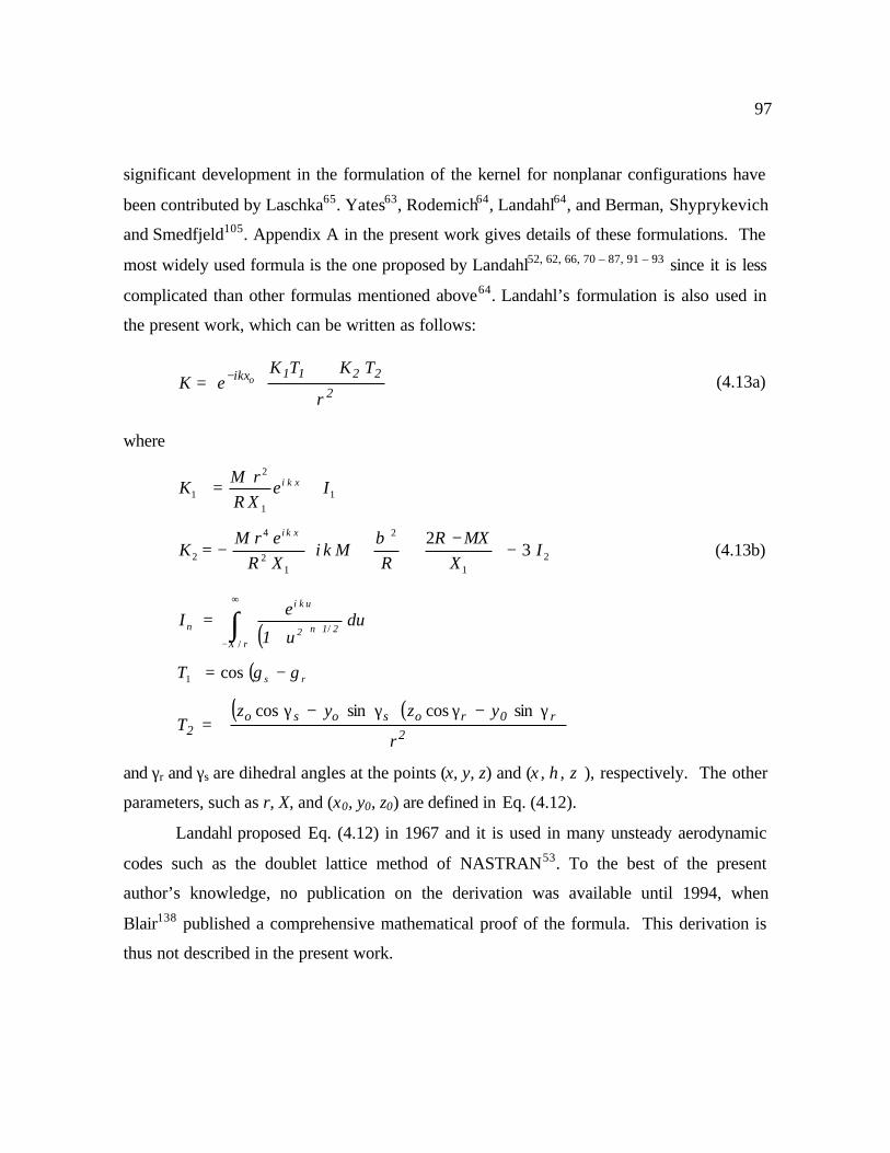
97
significant development in the formulation of the kernel for nonplanar configurations have
been contributed by Laschka65. Yates63, Rodemich64, Landahl64, and Berman, Shyprykevich
and Smedfjeld105. Appendix A in the present work gives details of these formulations. The
most widely used formula is the one proposed by Landahl52, 62, 66, 70 – 87, 91 – 93 since it is less
complicated than other formulas mentioned above64. Landahl’s formulation is also used in
the present work, which can be written as follows:
+= −
22211ikx
r
TKTKeK o (4.13a)
where
11
2
1 IeXRrM
K xki +=
21
2
12
4
2 32
IX
MXRR
MkiXRerM
Kxki
−
−++−=
β(4.13b)
( )du
u1
eI
rX21n2
uki
n ∫∞
−+
+=
//
( )rsT γγ −= cos1
( ) ( )2
r0rososo2
r
yzyzT
γ−γγ−γ=
sincossincos
and γr and γs are dihedral angles at the points (x, y, z) and (ξ, η, ζ ), respectively. The other
parameters, such as r, X, and (x0, y0, z0) are defined in Eq. (4.12).
Landahl proposed Eq. (4.12) in 1967 and it is used in many unsteady aerodynamic
codes such as the doublet lattice method of NASTRAN53. To the best of the present
author’s knowledge, no publication on the derivation was available until 1994, when
Blair138 published a comprehensive mathematical proof of the formula. This derivation is
thus not described in the present work.

98
4.2.3 Boundary Conditions
The pressure distribution on the lifting surface may be obtained by substitution of
Equations (4.7) or (4.8) into Equation (4.5) with the requirement that the solutions should
satisfy two boundary conditions, the so-called Kutta condition and the flow tangency
condition. The Kutta condition states that the pressure difference at the trailing edge of a
thin lifting surface must be zero. The flow tangency condition states that for an inviscid
flow the velocity vector must be tangent to the surface of the streamlined body.
4.2.4 Evaluation of the Kernel Function
The most critical part of calculating the kernel function in Equation (4.8) is the
evaluation of the so-called incomplete cylindrical function I1 and I2 occurring in Eq. (4.13).
Research, world wide, has been devoted to this problem during the last six decades. Some
of the formulas are listed in Table 1.4 of Chapter 1. The formulas may be classified into
two types:
Type-A( )∫
∞
−
++
==
rX
21n2
iku
n2n2n
n duu1
e
r
1
r
IB
/
/(4.14a)
Type-B ( )∫∞−
++=
X
21n22
uki
n duur
eB
/(4.14b)
where r and X are defined in Eq. (4.12).
The difference between the two types of the integrals may easily be seen for 0=r
and X < 0 where a direct calculation of nn rI 2/ by using the type A integral may give an
infinite result. The type-A integral was used earlier than the type-B in the formulation of
unsteady aerodynamic lifting surface methods. There are two reasons that motivated the
earlier usage of the type-A integral. The first reason is to simplify the evaluation of the
kernel function. It is shown in Eq. (4.13) that the parameter r2 is set as the denominator and

99
the incomplete cylindrical function In as the numerator. The usual approach in the past,
such as in the formulation of the doublet lattice method, was to assume that the numerator
can be approximated as a quadratic function. Or, in other words, the type-A integral form
is more suitable since the parameter r2 has already been extracted from the integral form. A
more detailed derivation of the doublet lattice method is given in Section 4.2.7 of the
present work. The second reason is because the analytical solution for the type-B was not
available before 1981. Therefore it was difficult to analytically separate the regular and
singular parts of the kernel function. In the present work, the type B integral is selected for
the formulation of the present lifting surface discrete element method.
Solutions to both type-A and type-B integrals have been reported using
approximation approach51, 102, 103, 151 and analytical approach78, 79. A summary of these
solutions is given in Table 1.4 of Chapter 1. The first attempt to perform analytical
integration of the incomplete cylindrical function was conducted by Laschka using a Taylor
expansion series102. However, he did not use his expansion series in his kernel function
method102 since he performed the integration only in the sub-interval [0, X] where the
singularities occurred in the real and imaginary parts of the series. Ueda in Refs. 77 and 78
performed analytical solution of the type B form by conducted the integration completely in
the sub-intervals [0, X] and [-∞, 0]. In his solution, the singularities occurring in the sub-
interval [0, X] and [-∞, 0] cancel out each other if X is negative. His solution coincide
exactly with the modified Bessel and Struve functions for a limiting case X = 0. For the
incomplete cylindrical function of order n, the Ueda’s expansion series can be written as
follows77, 78:
( ) ( ) imagnrealn
X
21n22
X
21n22n BiBduur
ukidu
ur
ukB ,,//
sincos+=
++
+= ∫∫
∞−
+
∞−
+(4.15)
where

100
∑∑∞
=
∞
=+−
−+−=
0n
n2
n
0n
v2
n2vn
realv vnn2rk
p1v22k
U1B)!(!
)/(!)!(
)/()( ,,
∑∑∞
=
∞
=
+ +−−
−−=
0n
n2
0n
v2
1n2vn
imagv vnn2rk
1v22k
2U1B
)!(!)/(
!)!()/(
)( ,,π
(4.16)
∑ ∑=
+
+=
++−−=n
1m
vn
1nm
n m21
m1
2k
p lnγ
γ = Euler’s constant = 0.577215664901532860606512…
and the U terms are based on the following recursion formulas :
2mv
2
1v21
1m
v2mv Umv2m
kr
Xmv2m
kXkU −−
−
≠ −−
−= ,, )(
)(
)(
)(
−
+−−= ∑=
−v
1m
1m2
11
v2
v2v XX
1m21
XXv2
kU )(ln
!, (4.17)
( )( )
( )( ) ( ) ( )
−−−++−
+−−−−
= ∑−−
=
++−−−
−<
1nv
0m
1n2m21
1mm1nv
nv2
n2
v2n2v 1nmvm1n2m2XXX1
1v21n2
2rn2
k1nvU
!!)/()(
!!!!
!
!)(,
( ) 1v21
1vX1v2
kU
−−−=,
and the symbol of double-factorials !! is used to define
( )12 −n !! = 1 •3. • 5 • 7… ( )1n2 − (4.18)
The analytical solution of the improper integral given in Eqs. (4.15) – (4.18) above
was proposed by Ueda in Refs. 77 and 78, but no derivation of the formulas is published
anywhere except in Ref. 135 where the present author derived the analytical solution
applicable for M < 1 (subsonic) flow.
One of the draw backs of the series given in Eqs. (4.15)-(4.18) is that the singularity
functions for r → 0 and X > 0 are not easily identified. In the present work, a further

101
analytical procedure to identify and separate the singular and regular parts is conducted. A
new alternate series proposed in the present work offers the possibility to unify the
treatment for the doublet-lattice and doublet point methods, the two well-known methods
for predicting the unsteady aerodynamic loads. More detailed derivations of the doublet-
lattice (DLM) and doublet point (DPM) methods are given in Sections 4.2.7 and 4.2.8
respectively. The present DLM and DPM methods are presented in Section 4.5 and 4.6
respectively.
4.2.5 Evaluation of the aerodynamic operator
The aerodynamic operator is a function relating the motion of the surface and the
change of the aerodynamic load produced by the surface deformation57. The definition of
the operator in the present work is similar to that used by Bisplinghoff and Ashley in Ref.
57 as follows
( )∫∫=ℑ
S
000 ddMkzyxKp81
ηξ∆π
,,,, (4.19)
where S is the lifting surface area.
There are many types of aeroelastic analyses which make use of this aerodynamic
operator. Among these are flutter, gust, and static aeroelastic analyses. The classical
approach to evaluate this operator has been through the use of the so-called lifting surface
methods. A vast literature on the methods to calculate the aerodynamic operator shows a
gradual improvement in the accuracy, capability and efficiency of the methods, as is
pointed out in the survey papers in References 52, 55, 68, and 69. The methods can be
divided into two broad categories, the mode function method (or the kernel function
method) and the discrete element method66. The mode function methods use an assumption
that the pressure distribution may be approximated by a series of orthogonal polynomial
functions with unknown coefficients. These coefficients are then determined by satisfying

102
the flow tangency boundary conditions at a set of collocation points.52, 69 For a wing with
control surfaces or other complex configurations, a careful treatment for the pressure
discontinuity is needed which makes this procedure sensitive to the manner of representing
the additional singularities associated with such geometry.
A usual procedure for the second method is to divide the lifting surfaces into small
trapezoidal panel elements which permit discrete approximation of Eq. (4.19) to give
( )∑ ∫∫=
=ℑ
N
1n S
000nn ddMkzyxKp81
ηξ∆π
,,,, (4.20)
If the normal wash can be calculated from the given oscillatory mode
shape ( )nnm yxh , by
( )nnm yxhkix
w ,
+
∂∂
= (4.20)
then the unknown pressure load, assumed to be constant within each element, may be
determined by satisfying the flow tangency condition at the control point of each panel to
give a set of linear algebraic equations :
{ } [ ] { }wp 1−ℑ=∆ (4.21)
In the discrete element method, the treatment for complex wing planforms is similar to
regular planforms, i.e. by dividing the planform into a number of small piecewise
trapezoidal panel elements, assuming an unknown constant ∆p for each panel, and finding
the unknown by satisfying the boundary condition on each panel. This discrete element
approach is used in the present work.

103
4.2.6 Discrete Element Lifting Surface Methods
Several variations of the discrete element method have been proposed. For steady
subsonic flow, one of the well known discrete element method is the vortex lattice method
(VLM), such as the method of Weissinger121, Falkner141, Campbell142, Hedman137,
Belotserkovskii140, Rubbert189, Dulmovits190, Margason and Lamar90, and Lan88,100. For
unsteady subsonic flow, these include the works of Stark52, Albano and Rodden70, Jordan71,
and Giesing et al.62, 67, 72, Houbolt73, Ueda and Dowell66, Ichikawa et al.74, Rodden et al.143-
145, and van Zyl 146-148. Application of the vortex lattice method to a high-angle-of-attack
subsonic aerodynamics has been proposed by Mook and Nayfeh.81
For a subsonic aeroelasticity analysis, the widely-used version of the unsteady
aerodynamics method is the doublet lattice method of Rodden et al.80 because of its ready
applicability to complex nonplanar configurations. NASTRAN53, 80 uses the DLM version
developed in Refs. 12, 17 and 22 where a quadratic approximation (DLM-quadratic) is used
for integrating the kernel function. Despite the wide acceptance of the method, however,
the DLM-quadratic version contains inaccuracy in the integration of the elemental kernel
function146, 147. For this reason, recently, Rodden et al. 143-145 attempted to improve the
accuracy by proposing a DLM-quartic version, where the integration of the kernel function
is based on a quartic function approximation. The DLM-quartic version143, 144 allows the
use of the element aspect ratio of up to 10, a considerable improvement compare to the
maximum aspect ratio of 3 for the DLM-quadratic. The DLM-quartic version , however,
still requires a large number of chordwise boxes per wavelength144. Reference 147
investigated the convergence of the DLM-quartic version and concluded that the limitation
of the DLM is as a result of the integration error introduced by the approximations to the
kernel numerators. In the present work, a more accurate DLM scheme using an analytical
integration of the singular kernel function is proposed. The details of the scheme are given
in Sections 4.3 – 4.8.

104
4.2.7 Doublet-Lattice Method (DLM) of Rodden et al.
There are four basic assumptions made in the application of the DLM-quadratic
version for subsonic flow:
First, the lifting pressure with an unknown constant strength is assumed to be concentrated
along the quarter chord line of each element surface as shown in Fig. 4.2. The flow
tangency boundary condition is satisfied at a control point placed at the three-quarter chord
along the center line of each element. Based on this assumption, if the control point is at
element j and the doublet line is at element i , then the aerodynamic operator in Equation
(4.16) may be replaced by
( ) ηζ−η−ξ−π
∆=ℑ ∫
+
−
ˆ,,,,8
dMkzyxKx
jijiji
e
e
sij (4.23)
where e is a semiwidth of the chordwise strip of each element
x
controlpoint
“receiving”panel
“sending”panel
doublet line
x
yΛ
e e
Figure 4.2. Lifting surface idealization in the doublet lattice method
Second, the lifting load line is represented by a horseshoe vortex for its steady effects, and
by a line of doublets for its incremental oscillatory effects. This assumption is used by

105
Albano et al.70 and Giesing et al. 62 to simplify the exact integration of the kernel for steady
part.
Therefore, for the steady part, the aerodynamic operator becomes
VLM
e
e
s dr
TKTKxℑ=η
⌡
⌠
+π
∆=ℑ
−
ˆ8 2
2201100 (4.24)
where VLMℑ is calculated based on the VLM of Hedman62. The symbol ^ indicates that the
local coordinates applied by Albano et al. in Reference 70 are to be used.
Third, for the planar part of the kernel, the spanwise integration is performed by
approximating the numerator of the kernel using a parabolic function.
η
+η+ηπ
∆=ℑ ∫−
ˆˆˆ
8 211
21
1 dr
CBAx e
e
s (4.25)
where
2111
1 2)()0(2)(
eePPeP
A+−−
=
eePeP
B2
)()( 111
−−= (4.26)
)0(11 PC =
and
1101
1 )tanˆ(exp)ˆ( TK
kixkiK
Pm
−
Λη+=η (4.27)
Fourth, for the nonplanar part of the kernel, Albano et al. 70 used the same procedure as for
the planar part, i.e.
η⌡
⌠
+η+ηπ
∆=ℑ
−
ˆˆˆ
8 222
22
2 dr
CBAxe
e
s (4.28)

106
The method gives a reasonable result for any arbitrary nonplanar interfering
surfaces, except for a near-coplanar wing-tail combination, such as the Cornell and
AGARD wing-horizontal tail combination 62, 67, 72. The refinement of the formula has been
achieved by Giesing et al. 62, 67, 72 by presenting a new dihedral angle correction factor
T2* = T2 r2 (4.29)
such that Equation ( 4.28) is replaced by
η⌡
⌠
+η+η
π∆
=ℑ
−
ˆˆˆ
8 422
22
2 dr
CBAxe
e
s (4.30)
where the parabolic function for the nonplanar part is
( ) ( ){ }[ ] *22022 tanˆexpˆ TKxikKP m −Λη+−=η (4.31)
The values of the kernel for k = 0 in Equations (4.27) and (4.31) are
( ) 122020
1010
22
1
−
−
β+−−=
−=
RrxK
RxK(4.32)
The formula of the kernel for unsteady motion have been given in Equation (4.9),
where the improper integrals are calculated by utilizing Laschka’s approximation series as
follows:
ikxeIikrXX
I
−+≅ 01
1 1
( )
+++
+−≅ ikxeJkrIikX
XXr
XX
ikXI 02
031
2
12 123
(4.33)
( )
+++
= ∑=
+
rX
ikrncikrncea
In
rncxn 111
1
/
0

107
( )
+++
= ∑= r
Xikrncikrnc
eaJ
n
rXnn 111
1
/372.0
0
where the coefficients an are given in Table 4.1.
The solution of the integral of planar part in Equation (4.21) is
( )[ ]
++
+++++−π
∆=ℑ −
−−
22
221
1111122
1 ln2
ˆ2ˆˆ8 zy
zyBAyeAFCByAzy
x
b
amm
s
(4.34)where
( )µ=
⌡
⌠+η−
η= −
−
122 tan
ˆ1
ˆˆˆ
ˆzzy
dF
e
e
p (4.35)
2ˆˆ2
zyy
ze
ba +=µ (4.36)
eyy
eyy
b
a
+=
−=
ˆ
ˆ
Table 4.1. The coefficients aI in Laschka approximation series
i ai i ai
1 0.24186198 7 -41.183630
2 -2.7918027 8 545.98537
3 24.991079 9 -644.78155
4 -111.59196 10 328.72755
5 271.43549 11 -64.279511
6 -305.75288
For planar surfaces, where 0=z , the Mangler principal part should be used, i.e.

108
( ) ba
e
e
p yyy
dF
11ˆˆ
ˆ2 −=
⌡
⌠η−
η=
−
(4.37)
In order to place the inverse tangent in the range [ ]π,0 , the working form of the F
term is written as:
( )zz
Fˆˆ
121
πδ+
ε−µδ= (4.38)
where
0/ˆ21,1
0/ˆ22/1,0
0/ˆ20,1
2
2
2
<µ=δ=δ
=µ=δ=δ
>µ=δ=δ
zefor
zefor
zefor
(4.39)
and
( )[ ]
<µµ−
−µ
>µµ
µ−
=ε
∑=
−
−
7
2
422
1
3.0ˆ12
)1(
3.0tan
1
n
nn
forzsignn
for
(4.40)
The solution for the integral of the non-planar part in Eq. (4.28) is
( )[ ] 101
forzy
F
zy
FFCByAzy
z16
xD
22a
22b
b222
222
s2 .
ˆˆˆˆˆˆˆ
ˆ<
+−
+++++=
µπ
∆
( )( ) ( )[ ] 101
forCByAzyzzyzy
Fz16
xD 222
222
122
b22
a
cs2 .ˆˆˆ
ˆˆˆˆˆˆ>
+++−
−++
=µ
∆εδπ
µ∆
(4.41)
where
( ) ( ){ } ( ) 222
22222 ˆˆˆˆˆˆˆˆˆ CyBzyyAezyyzyF aaa +++−−+=
( ) ( ){ } ( ) 222
22222 ˆˆˆˆˆˆˆˆˆ CyBzyyAezyyzyF bbb +++−++= (4.42)

109
( )( ) 22
222222 ˆ4ˆˆ2 BeyCAeezyFc ++++=
Applications of the numerical algorithm described above for complex
configurations have given good results compared to those of other methods and
experimental data62,67. There are, however, some limitations in the applications of the
method. Rodden et al. reported that the convergence of the method is slow for the real part
of the lift coefficient, and found that the computation converges if the strip-width of the
panel is approximately 25/λ , where k/2πλ = , and if the aspect ratio of each element is
approximately one. Therefore the method needs a large number of panels to give an
accurate result, and needs an appropriate numerical elimination procedure to handle a large
system of simultaneous equations.
In their analysis, Giesing et al.62 mentioned that the near-coplanar configuration
problem is not completely solved. The procedure fails, for example, if the separation z is
less than 0.001 e for a single precision code. For practical use, such configurations may be
assumed to be planar since the value of e itself is usually small. However, this indicates
that an effort to improve and optimize the method is still needed.
An effort to improve the accuracy of the method has been proposed by Jordan in
Ref. 71. In his DLM formulation, an exact integration of the kernel at a quarter chord of
the element has been done. However, this technique is limited to rectangular planar
surfaces in incompressible flow (M = 0). In the present work, several numerical
improvements are proposed, including an application of the exact solution of the improper
integral, a proper separation of the regular and singular functions of the kernel, and an
improve integration quadrature of the kernel.
The improper integral In in the DLM is solved using Laschka’s series to
approximate the integrand of the integral. There are two disadvantages to this scheme.
First, the accuracy of Laschka’s series is limited to the order of three digits. Second, the
series approximates the integrand, and not the integral itself. Gazzini et al. 82 described that
an approach to solve the integration by approximating the integrand may not be equivalent

110
to the approach to solve the integral itself. Therefore, it is believed that the application of
the exact solution to solve the improper integral directly will increase the accuracy of the
previous works.
The kernel function in Equation (4.12) contains regular and singular functions as the
values of r approaches zero and X > 0. There is no separation between these functions in
the DLM as shown in Equation (4.26), (4.27), (4.34) and (4.37). Therefore the Mangler
procedure is also applied to the regular function, which is not a proper way to solve the
problem. In the present work, the regular and singular functions will be identified and
treated separately.
The DLM uses a quadratic approximation for the numerator of the kernel to
simplify the integration procedure as shown in Equations (4.25) and (4.30). A further
approximation is also needed to evaluate the inverse tangent of the result as shown in
Equations (4.35) and (4.38) – (4.40) to give accurate results for small values of z. The
scheme clearly needs three integration points to form a quadratic approximation function
for every evaluation of the integral. This procedure may be improved if one uses a Gaussian
quadrature technique as is suggested by some authors 83-86. The Gaussian technique does
not need a fixed number of integration points. Less than three points may be used if the
sending/receiving panel pairs are distant. If the sending and receiving panels are close, such
that the kernel function may vary rapidly, one may have to use more than three integration
points. The improvements outlined above will be implemented in Section 4.7 of the present
work.
4.2.8 Doublet Point Method (DPM) of Ueda and Dowell
The idea of the DPM was first proposed by Houbolt81 based on the pressure-
velocity potential concept, and independently by Ueda and Dowell66 based on the pressure-
normal wash concept. Houbolt (1969), however, did not give numerical results for three-
dimensional flows since a direct evaluation of the type B integral in Equation (4.11) was

111
not available at that time. The exact solution of this type integral was given in 1981, and
the first version of DPM was developed in 1982 for planar surfaces66.
There are two basic assumptions used in the original DPM66. First, the lifting
pressure is assumed to be concentrated at a single point located at the three-quarter chord
along the center line of each element as shown in Fig. 4.3. The point is called a doublet
point. Similar to the DLM, the control point is placed on the three-quarter chord at mid-
span of each panel. Second, if the receiving point is located on the wake of the sending
element, i.e. X > 0 and r = 0, then the Mangler integration procedure should be used by
utilizing an average value of the modified Bessel function to treat the singularity problem.
x
Controlpoint
“receiving” panel
“sending”panel
doublet point
x
yΛ
e e
Figure 4.3. The lifting surface idealization in the doublet point method
Based on the first assumption, if the doublet point and the control point are located
at elements i and j respectively, then the aerodynamic operator in Equation (4.16) may be
written as

112
( )MkzyxKS
jijijii
ij ,,,,8
ζ−η−ξ−π
∆=ℑ (4.43)
where
ssi xeS ∆=∆ 2 = the area of sending element
The kernel function is calculated from Equations (4.8), (4.9), (4.10) and (4.12) for
planar surfaces
++= −
ir
ikXikx BiB
XReM
eK 111
0 (4.44)
and the improper integral B1 is calculated from Equations (4.13) and (4.14) for v = 1
( ) ( )( ) ( )
−γ−
++
+−−= ∑∑∑
=
∞
=
∞
=
n
m
n
nn
n
nr
kn
nmnnrkk
UB1
2
0
2
2,10
1 21
1211
1!2/
21
( ) ( )( )∑∑
∞
=
∞
=+ +
π+−=
0
2
0
2
12,11 !1!2/
41
n
n
nn
ni nn
rkkUB (4.45)
( )( )
( )( ) 2,1
2
1
1
3,1 2!2 −
−
≥ −−
−= m
m
m Umm
rkXmm
kXkU
( )
+−−=1
1
2
2,1 12 X
XXXn
kU (4.46)
11,1 X
kU −=
( )XXXU
−=
110,1
1
and
221 rXX += (4.47)
Equations (4.44)- (4.47) give an exact value of the kernel for any value of X and r
with one well known exception. Consider the case where the control point is downstream

113
of the doublet point, or X >0 and r = 0. The kernel becomes infinite because of the r -2
singularity in the part of B1,r or, more specifically, in the U1,0 term. This problem was
solved by Ueda and Dowell using the second assumption, which utilizes the Mangler
formula to integrate the B1, r term, and uses only the average value of the singular part.
( )( ) ( ) ( )( )
γ−−
+++
+++
+
η−+−=η>
∑∑∫∫
=
∞
=
−−
2ek
1n21n23n4
m1
1n21nn2ek
dXBe4
d0XB
n
1m1n
n2
e
er1
e
er1
ln!!
/
)()( ,,
(4.48)
If k e << 1, Eq. (4.48) can be simplified by
⌡
⌠η
−γ++−−=η>
−−∫
e
e
22r1
e
er1 d
23
2ek
ke
2XBd0XB ln)()( ,,
such that the value of the integrand B1,r may be replaced by
−γ++−−−≈>23
2ln
2)()0( 2
2,1,1ek
ke
XBXB rr (4.49)
Ueda and Dowell further improved the last equation to read
−γ++
π−−−≈>
23
2ln
6)()0( 2
2
2
,1,1ek
ke
XBXB rr (4.50)
Eversman and Pitt (1991) found that the averaging procedure used to give Equation
(4.46) is accurate only for element surfaces with uniform strip widths, e, as shown in Fig.
2.1a. In the case of unequal strip widths they suggested to include the strip width effect as
follows
( ) ( )
−γ++
+−−−≈>
23
2ln0 221
,1,1ke
ke
SSXBXB
irr (4.51)
where

114
( ) ( )
( )211
2
1
12
121
2
22
η+=
η−+
η−=
∑
∑ ∑∞
=
−
=
∞
+=
n
n
n
i
n
n
in
n
ye
S
ye
ye
S
(4.52)
Improvements to the DPM proposed in the present study includes a treatment of the
1/r4 term for nonplanar configurations which is not considered in the previous work, and an
evaluation of the sweep angle of elements for planar configurations which is neglected in
the DPM of Ueda and Dowell.
An appropriate treatment will be proposed to solve the ill conditioned problem of
the nonplanar 1/r4 term based on a separation of singular and regular functions of the
kernel. Ueda and Dowell66 have already made a separation of the kernel function in the B1r
term. However their approach did not completely separate the regular/singular functions in
the kernel function. If the separation is applied entirely to the singular kernel functions,
then it can be shown that the T1/r2 term of the planar term of the kernel function will cancel
the 4*2 /3 rT term of the nonplanar term. This treatment clearly will improve the accuracy
of the nonplanar DPM.
The original DPM used the Mangler procedure to evaluate the singular B1r term as
shown in Equation (4.44). This approach obviously evaluates only one part of the kernel
since the exponential term, exp (i k x0), is not included in the evaluation. In the present
DPM, the kernel will be evaluated completely through the use of the following equation
η= −
−∫ dBeK rikx
e
e1
0 (4.53)
where
( ) Λη−−= tan0 yxx m (4.54)

115
and Λ and xm are a sweep angle at the quarter chord of each panel and the distance between
the doublet point and the control point respectively. Since x0 is a function of the panel
sweep angle, this approach gives a sweep angle correction factor to the previous method.
4.2.9 Doublet Hybrid Method (DHM) of Eversman and Pitt
An extension of the DPM for nonplanar interfering surfaces has been made by
Eversman and Pitt75 based on the nonplanar kernel function of Landahl. In their work,
however, a treatment for the 1/r4 term of the nonplanar part of the kernel function was not
well established. The results have been reported to be less accurate than the DLM results.
For this reason, they concluded that the best approach is to utilize the nonplanar DPM only
for sending/receiving pairs which are distant. If the sending and receiving points are close,
they suggest using the nonplanar DLM. This combined technique is the basis of their
doublet hybrid method (DHM).
No further treatment for the limitation of DPM and DLM, was conducted in the
DHM method of the Eversman and Pitt. Therefore some singularity problems associated
with the DPM and DLM may be found in their DHM. In the present DHM, described in
Section. 4.7, the singularity problem is identified and solved in each of the present DPM
and DLM procedures. The present DHM also unifies the present DLM and DPM
procedures such that the present DPM is nothing more than just a special case of the present
DLM.
4.3. Contribution of the Present Work
The advantages and disadvantages of some the discrete element methods have been
described in the previous section. Most of the methods can handle complicated lifting
surface configurations. However, some mathematical integration and singularity problems

116
are not completely solved in the previous discrete element methods that may limit the
accuracy and applicability of the procedures. In the present work, three discrete element
methods are proposed: the DPM, DLM and DHM. Comparisons between the present and
previous methods are addressed in the following sections.
4.3.1 The doublet lattice method (DLM)
In the original DLM, the following problems have been identified:
1) The improper cylindrical function occurred in the kernel function is approximated using
the Laschka series which is third-order accurate (see Eq. (4.33))
2) No distinction is made between the regular and the singular parts of the kernel (see Eqs.
(4.24) and (4.30)).
3) The kernel is integrated based on a quadratic function approximation to the numerator
of the kernel (see Eqs. (4.24) and (4.30)). Recently Rodden et al. tried to improve the
solution of this part by using a quartic function approximation instead of the quadratic
function.
4) The non-planar kernel is integrated such that the denominator term is artificially set as
r-4 instead of r–2 (see Eq. 4.30). As pointed out by Nissim and Lottati93, such a
procedure may violate the behavior of the doublet singularity which should be r–2.
5) The scheme has a near singularity problem for two panels having small vertical gaps z.
In the present DLM, some improvement have been developed that cures the
problems above. The proposed DLM has the following features:
1) The improper cylindrical function is solved using an analytical expansion series
solution.
2) The kernel function is analytically separated into regular and singular functions.
3) The kernel singular part is integrated analytically. The kernel regular part is integrated
using a Gauss quadrature technique, where the accuracy can be improved simply by
increasing the number of integration points without the need to modify the formula.

117
4) The non-planar kernel is integrated without any artificial treatment for the denominator,
i.e. by retaining the r-2 term.
5) The singularity parts of the planar and non-planar kernel cancel each other in the
present formulation such that the kernel integration is continuous for any arbitrary
distance z of the vertical gap between two non-planar surfaces.
4.3.2 The doublet point method (DPM)
In the original DPM of Ueda and Dowell66, the following problems were described:
1) The method is applicable for planar lifting surface only.
2) The improper cylindrical function is solved using the analytical expansion series of
Ueda. However, it is difficult to isolate the singularity terms in the series since the
terms are implicitly embedded in the series.
3) No local sweep angle correction in the series.
4) It may not be accurate for non-uniform discretization of the surface planforms.
In the present DPM, some improvements have been made which alleviate the
problems associated with the original DPM.
The proposed DPM has the following features:
1) The DPM is extended to non-planar configurations.
2) The present solution series for the improper cylindrical function separately treats the
singular and regular functions. Therefore the singular part is explicitly isolated.
3) The sweep angle correction is included in the singular kernel.
4) Eversman and Pitt formula for the non-uniform spacing discretization is adopted.
4.3.3 The doublet hybrid method
In the original DHM of Eversman and Pitt75 , the following problems have been
identified:

118
1) The method utilizes the original DPM and DLM with the limitations described above.
2) For a steady flow, the VLM (for a small r) and DPM (for a large r) are used.
In the present DHM, some improvements have been made which alleviate the
problems faced by the original DHM.
The proposed DHM has the following features:
1) The present method utilizes the present DPM and DLM.
2) For a steady flow only the VLM is used for any value of r.
3) The DLM and DPM are unified such that the DPM becomes a special case of the DLM.
It should be noted that an effort to perform the present procedure has been initiated
by the present author in Ref. 135. The present work may be considered as an improvement
to the discrete element methods proposed in Ref. 135. The difference between the present
work and Ref. 135 are as follows:
1) The regular and singular kernel functions are separated using a different approach.
Reference 135 follows the approach proposed by Ueda and Dowel using the modified
Bessel functions. In the present work, the separation is performed analytically based on
an expansion series to the exponential function of the kernel function.
2) The procedure to separate the regular and singular kernel functions of the present work
can be performed to the incomplete cylindrical functions in both the frequency and
Laplace domains. The procedure in Ref. 135 is applicable for the frequency domain
only.
3) The regular kernel function of the present work is simpler since no additional term of
modified Bessel functions are included.
4) The discrete element methods of Ref. 135 may not be accurate for a high reduced
frequency since there is no treatment for the evaluation of the kernel function having
large arguments. In the present work, the treatment for a large argument is included
using an asymptotic expansion of the kernel function proposed in Ref. 78.

119
5) Reference 135 does not consider the influence of the reduced frequency k in the Gauss
integration of the regular function. In the present work, the number of integration point
is set as a function of the reduced frequency.
6) Reference 135 does not consider the effect of the lifting surface camber in the
formulation of the VLM. In the present formulation, the effect of the camber is
included.
7) The present work uses an alternate representation of the expansion series which is
simpler than the original series proposed by Ueda.
A schematic chart of the proposed treatment to the integration of the kernel
function, which is the key improvement of the present work, is given in Fig.E.1. and
described in Appendix A.
As a summary of the proposed discrete element methods, the following are the steps
conducted in the present work:
1) The kernel function is formulated based on the Landahl’s formula
2) The improper cylindrical function is solved using an expansion series described in
Appendix A.2.
3) The kernel function is divided into regular and singular functions as described in
Appendix A.3.
4) For the DPM, the kernel function is evaluated directly except for the singular case
where the singular kernel is integrated along the quarter chord using the Mangler
formula as given in Section 4.5. The method is applicable for steady or unsteady flows.
5) For the DLM, the singular kernel is integrated analytically and the regular kernel is
integrated using a Gauss quadrature formula as given in Section 4.6. The method is
applicable for steady or unsteady flows.
6) For the DHM, the treatment for steady and unsteady flow are separated as follows
a) For a steady flow, the present VLM is developed by considering the Prandtl-Glauert
compressibility correction in the governing equation as given in Section 4.4.

120
b) For the unsteady flow, the incremental unsteady portions of the present DLM and
DPM are employed as given in section 4.7.
7) Validation for the present discrete element methods are performed in Section 4.9.
4.4. Alternate Expansion Series for the Incomplete
Cylindrical Function
It has been described in Section 4.2 that the analytical solution to the incomplete
cylindrical function of order n has been given by Ueda 77, 78 as follows:
imagvrealvv BiBB ,, += (4.15)
where
∑∑∞
=
∞
=+−
−+−=
0n
n2
n
0n
v2
n2vn
realv vnn2rk
p1v22k
U1B)!(!
)/(!)!(
)/()( ,,
∑∑∞
=
∞
=
+ +−−
−−=
0n
n2
0n
v2
1n2vn
imagv vnn2rk
1v22k
2U1B
)!(!)/(
!)!()/(
)( ,,π
(4.16)
∑ ∑=
+
+=++
+−=
n
1m
vn
1nmn m2
1m1
2k
p lnγ
and the recursive term Um is defined in Eq. (4.17).
It is possible to further simplify the expression of the expansion series in Eqs. (4.15)
and (4.16) by combining the real and imaginary parts as follows:
∑∑∞
=
∞
= +−−
+=0n
n2
n0n
v2
nvn
v vnn2rk
p1v22k
UiB)!(!
)/(!)!(
)/( *, (4.58)
where
∑ ∑=
+
+=++
++−=n
1m
vn
1nmn m2
1m1
2i
2k
pπ
γ ln* (4.59)

121
and the recursive term Um is the same as the one defined in Eq. (4.17).
A more useful representation of the incomplete cylindrical function is by expressing
the function in terms of singular and regular parts as follows:
rvregularvv BBB singula,, += (4.60a)
where
→>+−
=otherwise0
0rand0Xifgg2XB ba
v)(
)(,singular
(4.60b)
+
→>−−−−+=
∑∞
=
otherwiseXB
0rand0XifXU12XBXB
v
0nn2
nv
ev
)(
)()()()(, gularr
where the singular functions ga and gb are
( ) !!!
ln1h2
hr
2k
gh2
a −
−= (4.61a)
n21h
0n
nh
2b 2rk
n1nh
1r
21h22
1g
−−
−
−
= ∑−
= !)!(
)(!)!(
(4.61b)
Equation (4.60) is used in the present work to develop the present lifting surface
method. A detailed derivation of Eq. (4.60) is given in Appendix A. It should be noted that
the expression for the alternate expansion series presented in Ref. 135 is more complicated
than the present expansion series. The alternate expansion series in Ref. 135 can be written
in the present notation as follows:
→>+−
=otherwise0
0rand0Xifgg2XB ba
v)(
)(,singular
(4.62a)
+→>+−−
=otherwiseXB
0rand0Xiff2XBXB
v
Rvev )(
)()(, gularr

122
where
( ) )()(!! bgagrk
rk
1v21
fv
R +−
−= vK (4.62b)
and Kv is the modified Bessel function of the second kind and order v defined as follows:
( )∑
∑∞
=
+
−−
=
+
++ϕ+ϕ
−+
−−
−+
γ+−=
0n
n2hh
hn21h
0n
n1h
hnn2kr
hnn21
2kr
n1nh
121
x2kr
1rk
)!(!)/(
)()()(
!!)(
)()(ln)()( hh IK
(4.62c)
Ih is the modified Bessel function of the first kind:
∑∞
=
+
+=
0n
n2h
hnn2kr
kr)!(!
)/()(hI (4.62d)
and ϕ is the Digamma function: 0)0(;1
)(1
=ϕ=ϕ ∑=
n
m mn (4.62e)
Therefore the present expansion series given in Eq. (4.61) can be considered to be
as a simplification of the expansion series given in Ref. 135. It should be noted also that
the alternate expansion series given in Ref. 135 is based on the assumption that the
argument of the modified Bessel functions in Eqs. (4.62c) aand (4.62d) is a real number,
i.e. it is applicable for the lifting surface method in the frequency domain only. On the
other hand, the present expansion series given in Eq. (4.61) is derived using a direct
expansion series to the exponential function in the incomplete cylindrical function without
any assumption on the argument of the modified Bessel function as shown in Appendix A.
Therefore the present formulation is applicable to the lifting surface method in the Laplace
domain where the argument of the incomplete cylindrical function is presented as a
complex variable. More detailed description on the Laplace domain approach is presented
in Section 4.9.

123
4.5 Present Vortex Lattice Method
In this section, the integration of the steady part of the kernel function is evaluated.
It has been known that an integration of the doublet line of the kernel is difficult to evaluate
directly, even for steady case. The integration has been accomplished by Jordan only for a
rectangular wing in an incompressible flow71. On the other hand, an integration of a similar
vortex distribution using a horseshoe vortex, the well-known vortex lattice method (VLM),
has been successfully completed for steady complex planforms100, 109, 110. The result for
steady rectangular surfaces has been proved to have the same form as those of Jordan71.
For this reason Albano and Rodden used the concept of the VLM to represent the steady
effects in their DLM70. Several versions of the VLM have been used including the version
of Weissinger121, Falkner141, Campbell142, Hedman137, Belotserkovskii140, Margason and
Lamar90, Rubbert189, Dulmovits190, Mook and Nayfeh81, and Lan88,100. The Hedman’s
version is used by Albano et al.70 and Giesing et al.62 to formulate the steady portion of
their DLM. In the present method, the VLM for non planar configuration is derived based
on the vector formulation given by Lan in the Appendix of Ref. 100. The formulation has
been initiated in the previous work of the author in Ref. 135 and is extended in the present
work by additional backwash velocity evaluation for a more general lifting surface with
camber.
In this approach, the surface is divided into trapezoidal panel element. Each panel is
represented by one horseshoe vortex. The vortex is composed of three vortex lines: a
bound vortex and two trailing vortices. The bound vortex is placed at the quarter chord of
each panel. The trailing vortices are places at the end of the bound vortex and are trailing
downstream in the free-stream direction to infinity. The control point is placed at the mid-
span of the three-quarter chord of each element. Figure 4.4. shows a typical chordwise row
of horseshoe vortices on an arbitrary planform.
Consider a vortex element Γ with an arbitrary direction lr
as shown in Figure 4.5.
The induced velocity field due to this vortex element in the linearized compressible flow

124
has been formulated by Lan100 based on the vector formulation given by Ward109. The
induced velocity is formulated as follows:
ββ
β
β
β
ββ
•
−∧
∧πΓβ
= la
a
b
b
la
la4
q2
2
r
rr
r
rr
rrr
(4.63)
where
x
controlpoint
“receiving”panel
“sending”panel bound vortex
x
yΛ
e e
trailing vortex
Figure 4.4 Lifting surface idealization in the vortex lattice method
kzjyixzyx
zzyy
xx
a acacac
ac
ac
ac
ca
ca
caˆˆˆ ++=
=
−−
−
=r
kzjyixb bcbcbcˆˆˆ ++=
r
kzjyixabl bababaˆˆˆ ++=−=
rrr
kzjyixa acacacˆˆˆ β+β+=β
r(4.64)
kzjyixb bcbcbcˆˆˆ β+β+=β
r

125
kzjyixabl bababaˆˆˆ β+β+=−=β
rrr
2M1 −=β , M < 1
and the symbols ∧ and • are used to define vector cross and dot products respectively. The
formula has been applied to planar configurations by Lan and is extended to construct his
quasi-vortex lattice method100.
A
B
Car
br
lr
Vortex line
control point
xy
z
Figure 4.5. Vortex segment geometry
The application of the formulation to a non-planar configuration surface with a
dihedral angle γ and camber surface angle δ should consider not only the downwash
velocity w but also the sidewash velocity v and the backwash velocity u110. These induced
velocities are related to the free-stream velocity from the surface boundary condition at
each control point as110
δγδγδγγδα sincoscossincoscoscos)sin( uvwU −+=−∞ (4.65)
The formulation to evaluate the downwash velocity w and sidewash v has been
described in Ref. 135. Reference 135 assumes that the camber angle δ = 0 such that there is
no need to evaluate the back wash velocity u. In the present work, the camber angle is not
zero, and therefore the formulation of the backwash velocity is needed.
The backwash u can be evaluated from Eq. (4.64)

126
iqurr
•= (4.66)
Substitution of Eqs. (4.63) and (4.64) into Eq. (4.66) gives
( ) acbabaac zyzyila −=•∧rrr
(4.67)
( ) ( ) ( )acbabaac2
acbabaacacbabaac zyzyzxzxyxyxla −β+−+−β=∧ ββrr
baac2
baac2
baac zzyyxxla β+β+=• ββrr
babc2
babc2
babc zzyyxxlb β+β+=ββrr
(4.68)
2ac
2ac
2ac
2 zyxa β+=βr
(4.69a)
2bc
2bc
2bc
2 zyxb β+=βr
(4.69b)
Therefore the backwash velocity can be formulated as
( ) ( ) ( )
( )( )
( )( )
++
++−
++
++
×−+−+−
+−=
−
ab2
ac22
bc2
acababac2
abac
cb2
bc22
bc2
bcababbc2
abbc
acababac2
acababacacababac
acababac1
zyßx
zzyyßxx
zyßx
zzyyßxx
zyzyßzxzxyxyx
zyzyp4
Gu
(4.70)
Similar procedure may be applied for the downwash w and sidewash v 135 :
( ) ( ) ( )
( )( )
( )( )
( )
( )
++−
++
++−
++
++
++−
++
++
×−+−+−
−=
−
bc2
bc22
bc2
bc
bc2
bc2
bc
ac2
ac22
ac2
ac
ac2
ac2
ac
ab2
ac22
bc2
acababac2
abac
cb2
bc22
bc2
bcababbc2
abbc
acababac2
acababacacababac
acababac1
zyßx
x1
zy
y
zyßx
x1
zy
y
zyßx
zzyyßxx
zyßx
zzyyßxx
zyzyßzxzxyxyx
yxyxp4G
w
(4.71)

127
( ) ( ) ( )
( )( )
( )( )
( )
( )
++−
+−
++−
++
++
++−
++
++
×−+−+−
+−=
−
bc2
bc22
bc2
bc
bc2
bc2
bc
ac2
ac22
ac2
ac
ac2
ac2
ac
ab2
ac22
bc2
acababac2
abac
cb2
bc22
bc2
bcababbc2
abbc
acababac2
acababacacababac
acababac1
zyßx
x1
zy
z
zyßx
x1
zy
z
zyßx
zzyyßxx
zyßx
zzyyßxx
zyzyßzxzxyxyx
zxzxp4
Gv
(4.72)
One may prove that the present non-planar VLM formulation is the same as the
trigonometric expression used by Giesing et al.62 based on the VLM of Hedman. For M = 0
and z = 0, or a planar incompressible case, the present formulation will reduce to the
expression given in Bertin and Smith110. For M = 0, or an incompressible case, the present
formulation will reduce to the expression given in Plotkin and Katz117. The present VLM
does not need any numerical integration procedure, and therefore does not add a significant
computational time to the unsteady aerodynamic calculation.
4.6 Present Doublet Point Method
Numerical improvements of the double point method (DPM) are presented in this
Section. The improvement is applied to the planar lifting surface configuration, and is
extended to the non-planar configurations. The numerical singularity problems of both
configurations are first identified, and then the solution procedures are described and
compared with the original solution of Ueda and Dowell66. The numerical results are given
in Section 4.9 and comparisons with other methods are discussed.
4.6.1 Present DPM for Planar Lifting Surfaces

128
The basic concepts of the original DPM are used here. The surfaces are divided into
small trapezoidal elements as shown in Fig. 4.3. The lifting pressure is assumed to be
concentrated at the doublet point located at the quarter chord along the midspan of each
panel. The control point is placed on the three-quarter chord at midspan of each element.
If the doublet point and the control point are located at elements i and j
respectively, then the aerodynamic operator may be written as
( )MkzyxK8S
jijijii
ij ,,,, ζ−η−ξ−π
∆=ℑ (4.73)
where the kernel function is based on Landahl’s formula64:
++= −
ir
ikXikx BiB
XReM
eK 111
0 (4.74)
The improper integral B1 in Eq. (4.74) is evaluated for the following two cases:
Case 1.
For the control point at a point ),,( zyx located outside the down stream panel of the
doublet point at a point (ξ,η,ζ ), i.e. for X < 0 or r > e, no singularity problem arises, and
therefore Eqs. (4.45) – (4.47) can be used directly.
Case 2
If the control point ),,( zyx is located at the center of the down stream panel of the doublet
point (ξ,η,ζ ), i.e. for X > 0 and r = 0, then the singularity problem arises. This can be
easily seen if the first two terms of the even series above is rewritten as follows:
++=
22201rX
X1
r
1U , (4.75a)
−++
+−= XrX
rX
X2k
U 2222
2
21 ln, (4.75b)

129
If r → 0, then X1 → X, and the kernel becomes infinite because of the strong dipole
singularity in Eq. (4.75a) and a weak logarithmic singularity in Eq. (4.75b). Ueda and
Dowell solved the problem by utilizing the Mangler formula to integrate the B1,r term, and
using the average value to the modified Bessel function as shown in Equation (4.44). In the
present work, a different approach is employed in the following two solution steps:
First, the basic form of the singularity part is identified and separated from the regular part.
Secondly, the Mangler procedure and the averaging rule is applied to the singular part only.
Based on a detailed derivation of the solution given in Appendix A.2 and E.4, the
final term of the formulation for the B1,r is rewritten as follows:
( ) ( ) Λγ 2222regular11 k
23
2ek
ke
2XB0XB tanln, −
−++−+=> (4.76)
where Bv, regular is given in Eq. (4.62). This result is slightly different than the formulation
given in Ref. 135 as follows:
( ) ( ) ( ) Λγ 2222imag1real11 k
23
2ek
ke
2XBiXB0XB tanln,, −
−++−+−−=>
Compared to the result of Ueda and Dowell in Eq. (4.49), which is rewritten in the
following:
( ) ( ) ( )
−++−+−−=>23
2ek
ke
2XBiXB0XB 2
2imag1real11 γln,, (4.49)
the present solution clearly gives a correction associated with the element sweep angle Λ.
The correction has a significant effect if the reduced frequency or the sweep angle is large.
The improvement proposed in Eq. (4.76) can be regarded as the answer to the question
arises in the technical comment by Rodden et al. to Ref. 66. Rodden et al. pointed out that
the DPM in Ref. 66 does not have the element sweep angle term. In their reply, Ueda and
Dowell66 acknowledged that their DPM indeed does not have an explicit sweep angle

130
correction but they suggested that the geometric arrangements of the doublet point may
implicitly give the sweep angle effect.
In the present formulation, the explicit sweep angle correction for each element is taken
into account as shown in Eq. (4.76). It should be noted that the term fU in Eq. (4.76) may
not add a significant computational time since we can use fU to evaluate B1,r in the same
time.
4.6.2 Present DPM for Nonplanar Lifting Surfaces
The method proposed in this section may be considered as an extension of the
planar DPM of Ueda and Dowell to nonplanar lifting surface configurations. In Ref. 75,
Eversman and Pitt have proposed the non-planar DPM. However, their method did not
specifically address a treatment for the 1/r4 near singularity problem in the nonplanar part
of the kernel. In the present work, an evaluation of the 1/r4 singularity problem will be
introduced and treated analytically.
Some basic concepts of the planar DPM are still used in the non-planar DPM
formulation. The lifting surface is idealized by dividing the surfaces into small trapezoidal
elements arranged in strips parallel to the free stream. The lifting pressure is assumed to be
concentrated at the doublet point located on the quarter chord at the midspan of each panel.
The control point is placed on the three-quarter chord at midspan of each element. There
are, however, at least three differences between the treatments for the planar and nonplanar
cases:
1. The fundamental difference is that, if the sending doublet lattice and receiving control
point are not in the same plane, the well-known singularity at r = 0 no longer appears.
2. For the non-planar configuration, there is an additional term, in the kernel function,
associated with the non-planar surfaces. The formulation becomes more complicated
because of two problems:

131
(i) the integration should be performed over both the planar and non-planar
surfaces,
(ii) the non planar kernel function involves a higher order of the incomplete
cylindrical function Bv, i.e. the order is v = 2.
3. The non-planar configuration has a three dimensional geometry. It is necessary to
perform a coordinate transformation from the global coordinate system into local
coordinate of each sending element in order to simplify the integration of the kernel
function.
The system coordinate is centered at the midpoint of the doublet lifting line and
rotating into the plane of sending element. The relations between the global coordinates
( ζηξ ,,,,, zyx ) and the local coordinates ( ζηξ ˆ,ˆ,ˆ,ˆ,ˆ,ˆ zyx ) are the same as the expressions
used in Appendix A.
If the doublet point and the control points are located at element i and j
respectively, then the aerodynamic operator may be written as
( )MkzyxKS
jijjij
ij ,,8 ,1, ζ−η−ξ−π
∆=ℑ (4.73)
where the kernel is based on the formulation of Landahl in the following notation
( )*2
*21
*1
0 TKTKeK xki −= − (4.77)
where
( )( )r0r0z0s02
i2r21
2
12
ikX
2
i1r11
ikX
1
yzyzT
Bi3B3X
XMR2R
MkiXR
eMK
BiBXReM
K
γ−γγ−γ=
++
−+
β+=
++=
sincossincos*
(4.78)
Note that the lateral distance, r is now for a three-dimensional coordinate defined as
20
20 zyr += (4.79)

132
Since 00 ≠z for nonplanar surfaces then consequently 0≠r , or the singularities no longer
appear. However, if the control point is at the center of the sending element wake, i.e.
000 >= Xandy , the value r becomes r = | z0 | and therefore is sensitive to the variations
of z0. If z0 << 1 this leads numerically to the near-singular problem, the solution of which
was not well established in the previous works.
The function B1 has been given in Equations (4.41) – (4.43). The functions B2 may
be obtained from Equations (4.15) – (4.17) for v=2.
( ) ( )( )( )
( ) ( )( )∑∑
∑∑∑∞
=
∞
=
+
=
∞
=
∞
=
+π
−−=
−γ−
+++
+×+
+−=
0n
n24
0n
1n22n
i2
n
1m0n
4
n22n
0n
r2
2nn2rk
24k
U1B
2k
n12n1n2
3n2m1
2nn2rk
12k
U1B
!!/
)!(!/
,
,
(4.80)
where
( )( )
( )( ) 2m2
2
31
1m
4m2 Um4m
rk
Xm4m
kXkU −
−
≠ −−
−= ,,
!
( )
++−−= 2
1
2
11
4
42X3
X1
XX
XX6k
U ln,
( )
+−
=11
31
22
22 X1
xXX
X6k
U , (4.81)
31
12X3
kU −=,
( )21
3i
102
XXX3
XX2U
−
−=,
and
221 rXX += (4.47)

133
For the case of X > 0 and r << 1, the value of X1 approaches X and a nearly –
singular problem can be seen in the zeroth, second, and fourth order terms of the U series.
Analytical solution to this problem is described in Appendices E.2 to E.4. Therefore, two
different treatments are employed for the kernel. The final forms for each case is as
follows:
Case 1
Case 1 is for most of the cases of the sending and receiving point pairs, i.e. for the control
point not directly located in downstream of the doublet point, or more specifically, for
• X < 0 and arbitrary r
• X > 0 and r > e
In this case Eqs. (4.78) – (4.81) can be used directly since no singularity arises.
Case 2
For the control point directly behind the control point, the kernel is evaluated as follows
( ) ∑∞
=
+−
−
+−
λ+−=
0n
n2n
2
n
n1
reg2reg21reg1xki f
1n2Vk
Vnne2
cTKTKeK 0
)(!*,
*,
*, (4.82)
where
+−π=
=
−−−
=
−
−
−−
>
2m
21
0
a
b1
2n2
1na
1nb
1n
re
ze2z1
V
rr
V
Vz1nyy
V
|ˆ|tan
|ˆ|
ln
ˆ
(4.83)

134
bj
aj
j2
j
1njn 1n2
rk
r1
yf
=
=
+
+−=
)(
ln(4.84)
mxkisr1 e2c
ki−γ−γ=
Λ−=λ
)(cos
tan(4.85)
222222222 ˆˆ;ˆ;ˆ
ˆ;ˆ
zyrzyrzyr
eyyeyy
mbbaa
ba
+=+=+=
+=−=(4.86)
The regular part of the kernel function is evaluated as follows:
regular11
Xki
reg1 BXR
eMK ,, += (4.87a)
regular21
2
12
Xki
reg2 B3X
XMR2R
MkiXR
eMK ,, +
−++=
β(4.87b)
where Bv, regular is given in Eq. (4.62).
It should be noted that the present regular kernel function is simpler than the one
given in Ref. 135. The regular kernel function used in Ref. 135 can be written in Eqs.
(4.88) – (4.90) as follows:
)()( *,
*,, XBiXB
XReM
K imag1real11
Xki
reg1 +−+= (4.88a)
)()( *,
*,, XB3iXB3
XXMR2
RMki
XR
eMK imag2real2
1
2
12
Xki
reg2 +−+
−++=
β(4.88b)
where the second expansion series is slightly different than the Ueda series as follows:
( ) ( )( ) ( )
−−−
++
+−−= ∑∑∑
=
∞
=
∞
=
n
1m1n
n22
0nn21
nreal1 r2
2k
n11n2
1m1
1nn2rk
2k
U1B ln!!
/*,
*, γ

135
( ) ( )( ) ( )( )
−−
+++
++
−−= ∑∑∑=
∞
=
∞
=rn12
2k
2n1n23n2
m1
2nn2rk
12k
U1Bn
1m0n
n24
0nn22
2real2 ln
!!/*
,*, γ
imag1imag1 BB ,*, =
imag2imag2 BB ,* =
The recursive series U*n for the first order n = 1 are
( )( )
( )( )
*,
*, ! 2m1
2
1
1m
3m1 Um2m
rkXm2m
kXkU −
−
≥ −−
−=
( )
+−+=1
1
2
21 XX
XX2k
U ln*, (4.89)
and for the second order n = 2, are as follows:
( )( )
( )( )
*,
*,
!2m2
2
31
1m
4m2 Um4m
rk
Xm4m
kXkU −
−
≠ −−
−=
( )
+++= 2
1
2
11
4
42X3
X1
XX
XX6k
U ln*,
( )
++
−=11
31
22*
2,2
16 XXXX
XkU
( )
−γ++
++
=43
21
1232 4
21
31
1*0,2
kn
kXXX
XXU (4.90)
Equations (4.82) – (4.87) are the final expression used to evaluate the kernel for
nonplanar configurations. In contrast to the solution given by Rodden et al. in their second
version of the DLM 72, the result presented here is finite for any arbitrary value of z. In
their work, the singular parts of the planar and nonplanar terms functions cancel out each
other only for limiting values of the kernel, and the cancellation of these singularities

136
numerically will lead to difficulties for sufficiently small values of z. In the present work,
the singular parts are eliminated not only for the limiting case, but also for any value of r.
4.7 Present Doublet Lattice MethodNumerical improvements of the double lattice method (DLM) are presented in this
chapter. The improvements are applied to two types of lifting surface configurations,
including the planar lifting surface and the non-planar lifting surface configurations. The
numerical singularity problem of both configurations are first identified, and the solution
procedures are described and compared with the original solution of Albano and Rodden70
and with it’s refinement solution proposed by Rodden, Giesing and Kalman72. The
numerical results are given in Section 4.8 and comparisons with other methods are
discussed.
x
controlpoint
“receiving”panel
“sending”panel
doublet line
x
y
Λ
e eGauss integrationpoints
Figure 4.6. Lifting surface discritezation in the present doublet lattice method

137
4.7.1 Present DLM for Planar Lifting Surfaces
The basic concepts of the original DLM are used here. The surfaces are divided
into small trapezoidal elements as shown in Fig. 4.6. The lifting pressure is assumed to be
concentrated at the doublet lifting line located at the quarter chord of each panel. The
control point is placed on the three-quarter chord at mid-span of each element.
If the doublet lifting line and the control point are located at elements i and j
respectively, then the aerodynamic operator may be written as:
( ) ηζ−η−ξ−π
∆=ℑ ∫−
dMkzyxKx
jijiji
e
e
sij ,,,,
8(4.91)
In the original DLM, the numerical integration of the kernel function K is based on
the quadratic approximation of the numerator as shown in Equation (4.25). In the present
work, the integration procedures are based on the following procedure:
1) The improper cylindrical function contained in the kernel function is solved analytically
by using an expansion series. This step is described in Appendix A.3.
2) Analytically separate the kernel function into two parts: the regular and singular parts
3) Perform an exact integration solution for the singular part of the kernel, and
4) Perform a Gaussian quadrature integration for the regular part of the kernel
Based on the steps outlined above, the aerodynamic operator can be derived as follows:
( )
+η
π∆
=ℑ ∫ ∑=
N
nnngerg
sji WKdK
x
2sin8
(4.92)
where Wn is the Gauss-Legendre weighting factor, and N is the number of integration
points. This number is not fixed and may be increased to improve the accuracy. In the
present work, N is selected based on the distance r, the wing root chord croot, the reduced
frequency k, and X as shown in Table 4.1. The weighting factor, Wn can be obtained in Ref.
166.

138
Table 4.1. The number of Gauss integration points N
rg = 2 r / croot k X < 0 X > 0
0 < rg < 0.1 4 7
0.1 < rg < 0.25 4 6
0.25 < rg < 0.5 3 5
0.5 < rg < 1.0 3 4
1.0 < rg < 2.0 2 3
rg > 3.0 2 2
The Gauss-Legendre technique uses the expression of the integrand directly,
without any additional weighting function. Therefore a direct evaluation of the kernel, such
as the type B integral in Equation (4.11), can be applied directly. For this reason, the
present method uses the new expansion series, described in detail in Appendix A.3, to
evaluate the improper integral. Compared to the Laschka’s approximation used in the
previous DLM, the present series is an exact representation of the incomplete cylindrical
function. The present expansion series is almost similar to the Ueda’s expansion series
except that the present series explicitly separates the singular and regular kernel functions
such that the kernel function integration can be performed more easily.
Based on the derivation described in Appendix A.4, the final form for the present
DLM are as follows:
The regular part of the kernel function can be obtained as follows:
( )n
xkinreg efK η=η=η=η 0
1 (4.93)
where

139
−+++=
21
2k
kBRX
eMf 2
regular11
ikX
1 γln, (4.94)
and the improper cylindrical function B1 is given by Eqs. (4.45)-(4.47). It is important that
the absolute value of X in the third term of the right-hand side of Eq. (4.94) is intended to
set the series into a regular function for every value of X.
Equation (4.94) is almost similar to the formulation given in Ref. 135 given as
follows:
( ) ( )
−++−++=
21
2k
kXBXBiRX
eMf 2
r1i11
ikX
1 γln,,
The singular part of the kernel function is integrated using the Mangler’s technique
as shown in Appendix A.4. The closed form solution of the integration is
( ) ( )
+
−−
Λ+
ΛΛ
×=η
∑
∫∞
=
−
−
2
2
0
sin
)12()12(2
)!2(tan
lntan
tansin
2ˆ
nek
nenkei
ekke
edK
n
xikg
e
e
m
(4.95)
One may prove that there is no singular term in this final equation. Therefore it eliminates
the need to apply a special treatment for the near singularity problem.
4.7.2 The present DLM for Nonplanar Lifting Surface Configurations
Some basic concepts of the planar DLM are still used in the non-planar DLM
formulation. The lifting surface is idealized by dividing the surfaces into small trapezoidal
elements arranged in strips parallel to the free stream. The lifting pressure is assumed to be
concentrated at the doublet lifting line located at the quarter chord of each panel. The
control point is placed on the three-quarter chord at midspan of each element.
If the doublet lifting line and the control point are located in panels i and j
respectively, then the aerodynamic operator may be written as:

140
( ) ηζ−η−ξ−π
∆=ℑ ∫−
dMkzyxKx
jijiji
e
e
sij ,,,,
8(4.96)
Analytical solution to this problem is described in Appendices E.2 to E.4. Two
different treatments are employed for the kernel. The final forms for each case is as
follows:
Case 1
Case 1 is for most of the cases of the sending and receiving point pairs, i.e. for the control
point not directly located in downstream of the doublet point, or more specifically, for
• X < 0 and arbitrary r
• X > 0 and r > e
In this case Eqs. (4.78) – (4.81) can be used directly since no singularity arises, i.e.
nn
N
2n
sij WK
8x ∑
=π∆
=ℑ (4.97)
Case 2
The integral procedure of the kernel is similar to those of the planar method in the
previous section which employed an exact integration procedure to the singular part, and
Gauss-Legendre integration technique to the regular part.
∫ ( )
+=ℑ ∑
=−nnregular
N
2n
e
e
sij WKdK
8x
ηπ
∆singular (4.98)
where Wn is the Gauss-Legendre weighting factor, and N is the number of integration points
as shown in Table 4.1.
The regular part of the kernel function in Eq. (4.98) is evaluated as follows:
( )2211xki
regular TKTKeK 0 ** −= − (4.99)
where

141
224
21
2
12
ikX
reg2
11
kXi
reg1
krr4k
B3X
XMR2R
MkiXR
eMK
BXReM
K
−++
−+
β+=
+=
ln*,
*,
(4.100)
and the B* function is given by Eqs. (4.88) – (4.90).
The singular part of the kernel function in Eq. (4.98) is evaluated as follows:
n0n
n
1g
e
eW
ncdK ∑
∞
=
+
−
λ=η⌡
⌠!sin (4.101)
where
)()(ˆtanˆ afbfVznVVnW 551n2nnn −+γ+−= −+ (4.102)
( )2
t
1nt
t1n
t
2
5r
y1zry
1n2k
tf+
+ −γ++
= ˆtanˆln)(
)( (4.103)
One may find that the non-planar formulation above gives a finite result for any value of r,
including for the case X > 0 and r → 0, i.e. when the control point is near the center of the
wake. Since the singularity problem is identified and separated analytically, the near
singularity problem vanishes and the results are continuous and finite for any arbitrary
value of z.
4.8 Present Doublet Hybrid MethodIn the present doublet hybrid method (DHM), the aerodynamic load is calculated
based on a hybrid of three different methods: the vortex lattice method (VLM), the doublet
lattice method (DLM), and the doublet point method (DPM). The vortex lattice method is
used for the steady part since the method performs exact integration of all terms of the
kernel function. For the incremental unsteady part of the kernel, both doublet methods are
used. The DPM is used if the kernel function is nearly constant across the element. The

142
DLM is used if the kernel function varies considerably across the element. Since the
function is closely related to lateral distance r of sending and receiving points, the doublet
methods chosen are based on r as shown in Table 4.3.
Table 4.3
List of procedures used in the doublet hybrid method
Unsteady Flow ( k > 0 )rg = 2 r / croot k
Steady flow
( k = 0 ) X < 0 X > 0
0 < rg < 0.1 VLM DLM with N = 4 DLM with N = 7
0.1 < rg < 0.25 VLM DLM with N = 4 DLM with N = 6
0.25 < rg < 0.5 VLM DLM with N = 3 DLM with N = 5
0.5 < rg < 1.0 VLM DLM with N = 2 DLM with N = 4
1.0 < rg < 2.0 VLM DLM with N = 2
rg > 3.0 VLM DPM
Based on Table 4.3., the aerodynamic operator is formulated as follows:
( )MkzyxK8x
jijijii
ij ,,,, ζ−η−ξ−π
∆=ℑ (4.104)
where the kernel function K is formulated in the following equation
( )( )( )
=−+
><=−+
>=−+
=
casesotherallfor0kKKK
0Xand2erfor0kKKK
Xanyand3rfor0kKKK
K
DLMVLM
DLMVLM
DPMVLM
)(
/)(
)(** (4.105)

143
The Vortex Lattice Method
The kernel function KVLM in Eq. (4.105) is the same as the kernel function for the
present vortex lattice method described in Section 4.4. The formula is not rewritten here
since it can be used directly for the present DHM.
The Doublet Point Method
The kernel function KDPM in Eq. (4.105) is the same as the kernel function for the
present DPM Case 1 (no singularity case) described in Sections 4.6.1. and 4.6.2. The
kernel function KDPM (k=0) is the steady part of the kernel by setting k = 0. The results for
planar configuration is as follows:
( ) 2111
21)0(
eXXXXRM
kK −+
−== (4.106)
For nonplanar configurations the steady part of the kernel is given as:
( ) ( ) ( )
−
γ−=−Τ===
2a
a2b
b2reg21reg1
r
y
r
ye
T0kK0kK0kKcos
,, (4.107)
( ))(, XXX
1XR
M0kK
111reg1 +
−== (4.108)
( )2
131
1
1
2
12reg2
XXX
XX2X
XMR2RXR
M0kK
)(,
+
+−
−+
β== (4.109)
The Doublet Lattice Method
The kernel function KDLM in Eq. (4.105) is the same as the kernel function for the
present DLM Case 1 (no singularity case) and Case 2 (singularity case) described in
Sections 4.7.1. and 4.7.2. The kernel function KDLM (k=0) is the steady part of the kernel
by setting k = 0. The integration of the kernel is performed as follows:

144
( ) ( )
=−+η=−
π∆
=ℑ ∑∫=−
N
2n
nnregreg
e
e
ggs
ji W0kKKd0kKK8x
)()(sinsin (4.110)
where the steady part for the kernel in planar configuration are
e4
d0kK
e
e
g −=η=∫−
)(sin (4.111)
( ))( XXX
1XR
M0kK
111reg +
−== (4.112)
The steady part for the kernel in non-planar configuration are
−γ−=η=∫
−
2a
a2b
b
e
e
gr
y
r
y2d0kK ˆcos)(sin (4.113)
( ) ( ) ( ) 2reg21reg1reg T0kK0kK0kK =−Τ=== ,, (4.114)
where
( ))(, XXX
1XR
M0kK
111reg1 +
−== (4.115)
( )2
131
1
1
2
12reg2
XXX
XX2X
XMR2RXR
M0kK
)(,
+
+−
−+
β== (4.116)
4.9 Unsteady Aerodynamic Load in Laplace DomainThe basic lifting surface theory and numerical solution methods described in
previous sections are derived based on the so-called frequency domain approach, where the
velocity potential ϕ(t) is assumed to oscillate following the lifting surface harmonic motion
about its equilibrium as shown in Eqs. (4.3) and (4.6). Attempts to predict unsteady
aerodynamic loads for a more general type of motion have also been initiated since six

145
decades ago179. The procedures for constructing aerodynamic loads for general motions
can be divided into two different approach: the aerodynamic transfer function method179 -
182, and the Laplace domain aerodynamic method136, 183, 184. A typical technique in the
aerodynamic transfer function method is to utilize the aerodynamic loads obtained in the
frequency domain. If the general motion is represented in the Laplace domain, then the
harmonic unsteady aerodynamic load can be interpreted as the loads on the imaginary axis
in the complex s-plane. The aerodynamic transfer function can be constructed such that the
approximation curve fits the harmonic load data in the imaginary axis180, 181. This approach
is obviously limited to the proximity of the imaginary axis and needs a number of
aerodynamic frequency domain results to give accurate approximation.
The other approach formulates the unsteady aerodynamic loads directly in the
Laplace domain136, 183, 184. This approach gives an analytical expression of the aerodynamic
load in the complex s-plane without any curve fitting approximation, and, therefore,
reduces the computational time without degrading the accuracy. The possibility of
implementing this approach to the present lifting surface methods is shown in the next two
Sections.
4.9.1 Kernel Function Formulation
Similar to the Kussner normal wash-pressure equation in frequency domain given
by Eq. (4.8), the integral equation in the Laplace domain, that relates the normal wash w at
a point (x, y, z) to a pressure difference p∆ on an infinitesimal area dξ dη centered at a
point (ξ, η, ζ ), can be formulated as follows:
( )∫∫ ηξ∆π
=S
0oo ddMhzyxKp81
w ,,,, (4.117)
where h is the non-dimensional Laplace transform variable defined as:
∞=+=
Ubs
kiah (4.118)

146
and s, a and k are the dimensional variable of the Laplace transform, its non-dimensional
real part and imaginary part, respectively. The function K represents the kernel function in
Laplace domain which has been formulated by Ueda184 as follows:
+= −
22211hx
r
TKTKeK o (4.119)
where
ζ−=η−=ξ−=
zzyyxx
o
o
o
2o
2o zyr +=
222 rxR β+=
( ) 2o RMxX −β−= (4.120)
221 rXX +=
2M1 −=β
1xh
1
2
1 IeXRrM
K +=
21
2
12
xh4
2 I3X
MXR2R
MhXR
erMK −
−+
β+−=
( )du
u1
eI
rX21v2
uh
v ∫∞
−+
+=
//
( )rsT γγ −= cos1
( ) ( )2
r0rososo2
r
yzyzT
γ−γγ−γ=
sincossincos

147
and γr and γs are dihedral angles at the points (x, y, z) and (ξ, η, ζ ), respectively.
One may find that this kernel function formulation in the Laplace domain given by
Eq. (4.119) will reduce to the kernel function formulation in frequency domain given by
Eq. (4.12) if the real part of the Laplace domain a approaches zero. In other words, the
pressure distribution calculated based on Eq. (4.119) will fit the pressure distribution based
on Eq. (4.12) in the imaginary axis of the complex s-plane.
4.9.2 Incomplete Cylindrical Function
Similar to the kernel function formulation for the frequency domain, the incomplete
cylindrical function I1 and I2 occur in Eq. (4.120) with a complex variable h. In the present
formulation, the type-B integral is written as:
( )∫∞−
++=
X
21v22
uh
v duur
eB
/(4.121)
where the integral Bv and Iv are related as follows:
( )∫∞
−+
+==
rX21v2
hu
v2v2v
v duu1
e
r
1
r
IB
//
(4.122)
The analytical solution of the type B integral has been given by Ueda 184 in the
following infinite series:
∑∑∞
=
∞
= +−
−+=
0n
n2
nn
0n
v2
nvv vnn2rh
p11v2
2hUXrhB
)!(!)/(
)(!)!(
)/(),,( , (4.123)
where
∑ ∑=
+
+=++−γ−=
n
1m
vn
1nmn m2
1m1
2h
p ln*
γ* = Euler’s constant = 0.577215664901532860606512…
2nv
2
1v21
1n
v2nv Unv2n
rh
Xnv2n
XhhU −−
−
≠ −−
−= ,, )(
)(
!)(
)(

148
−
+−−= ∑=
−
=
v
1m
1m2
11
v2
v2nv XX
1m21
XXv2
hU )(ln
!, (4.124)
( )( )
( )( ) ( ) ( )
−−−++−
+−−−−
= ∑−−
=
++−−−
−<
1nv
0m
1n2m21
1mm1nv
nv2
n2
v2n2v 1nmvm1n2m2XXX1
1v21n2
2rn2
h1nvU
!!)/()(
!!!!
!
!)(,
( ) 1v21
1vX1v2
hU
−−−=,
and the symbol of double-factorials !! is used to define
!!)()(
!!)(
)...(!!)(
1n21
n21
1n25311n2n
−−
=−−
−•••=−
(4.125)
The expansion series of the incomplete cylindrical function in Laplace domain
given by Eqs. (4.123)-(4.125) is similar to the expansion series in frequency domain given
by Eqs. (4.15)-(4.16). Therefore the treatment to identify and separate the regular and
singular parts of the kernel function is also similar to the treatment for the frequency
domain, but with one exception: the logarithmic function with a complex argument ln(h)
appearing in Eq. (4.124) should be evaluated as
++=+ −
ak
ikakia 122 tanln)(ln (4.126)
To prove that the expansion series of the Laplace domain in the imaginary axis will
give the same expansion series of the frequency domain, we can set the real part of the
Laplace domain a in Eq. (4.126) to zero:
kih = for a = 0 (4.127)
such that Eq. (4.126) becomes
2ikkia
π+=+ ln)(ln for a = 0 (4.128)

149
Substitution of Eq. (4.128) into Eq. (4.124) will yield the same expression as Eqs. (4.15)
and (4.16). This similarity offers the same treatment for the application of the kernel
function in the Laplace domain to the present lifting surface methods, i.e. the same
procedures can be used: identification and separation of the regular and singular parts of the
kernel function, exact integration to the singular part of the kernel function, and Gauss
quadrature integration to the regular part of the kernel function.
4.9.3 Application to the Strut-Braced Wing Aeroelastic Analysis
The unsteady aerodynamic load prediction in the Laplace domain is important in the
strut-braced wing analysis to study its nonlinear aeroelastic response. It has been explained
in Chapters 1 and 2 that, because of the compressive force effect, the aeroelastic response
of the strut braced wing is more complicated than the conventional cantilever wing. By
considering the other aerodynamic loads such as the wind gust, the aeroelastic equation for
the strut braced wing can be written as:
( ) )()()(),()( ttxtxxxtx eag FFKP-KM =−+ &&&& (4.129)
where P is the compressive force generated by the strut, M, K and Kg are the mass,
stiffness and geometric stiffness matrices respectively, and Fa and Fe are the self-excited
and external aerodynamic forces respectively.
The compressive force P in Eq. (4.129) is a function of displacement of motion
since the strut-braced wing is an indeterminate structure. P is also a function of the
acceleration of motion since, in the present strut braced wing, the strut is activated if the
flight load factor is greater than 0.8 g. If the external aerodynamic force Fe, such as a gust
load, excites the structure with a considerable positive and negative load factor, the strut
will be engaged and disengaged during the motion to prevent the strut buckling. Therefore,
Eq.(4.129) becomes a nonlinear equation where it is unlikely that the wing vibrates
harmonically.

150
To calculate the aeroelastic response of the system, the present lifting surface
method in the frequency domain can be used to construct the self-excited force Fe.
However, to generate a non-harmonic force, the frequency domain approach needs a
considerable amount of calculation to approximate the load. On the other hand, the present
lifting surface method in the Laplace domain offers the possibility to directly calculate the
non-harmonic force Fe and calculate the response in Laplace or time domain. This
aeroelastic response analysis deserve further intense investigation, and is not conducted in
the present work.

151
4.10 Validation
To implement the theoretical development of the present lifting surface methods, a
FORTRAN computer code was developed and presented in Appendix A. To evaluate the
accuracy of the present methods, a number of wing planforms are used and the results are
compared with experimentation data or other lifting surface method results.
4.10.1 Delta Wing with AR=2
Table 4.4. Lift coefficient CL of a delta wing with AR=2 and α= 4.3°
Nx x Nyaerodynamic panel Present DPM Present DLM Present DHM
1 x 20 0.1662 0.1635 0.1636
2 x 20 0.1678 0.1653 0.1651
3 x 20 0.1681 0.1655 0.1652
4 x 20 0.1682 0.1657 0.1655
5 x 20 0.1683 0.1657 0.1655
Experiment124 0.159
Margason and Lamar90 (6 x 20) 0.1654
Lan100 (3 x 35) 0.1649
Lamar119 (4 x 11) 0.168
Nissim and Lottati92 (3 x 3) 0.1626
Dulmovits119 0.165
Wagner120 0.1663

152
The first example is a delta wing with AR = 2 shown in Fig. 4.7. This wing
planform has been selected by many to demonstrate their numerical procedures as shown in
Table 4.4. Experimentation data is based on Wick124. The experimentation was performed
in a steady flow with Mach number 0.13, Reynolds number 2.4 million. The results
obtained using the present methods, shown in Table 4.4 and Figure 4.7, are in a good
agreement with other lifting surface methods and experiments results. Note that the
convergence rate of the present DPM result with respect to the number of panel element is
slower than the present DLM and DHM.
0
0.2
0.4
0.6
0.8
1
1.2
1.4
0 0.2 0.4 0.6 0.8 1spanwise y/b
cl(y
) c(
y)/ C
L c
avg
Present DPM
Present VLM
VLM (NASTRAN)
Figure 4.7 Spanwise lift distribution of a delta wing with AR=2 and M=0.13

153
4.10.2. Double-Delta Wing
To demonstrate the accuracy of the present VLM for evaluating a more complicated
planform, a cropped double-delta wing is selected. The aerodynamic pressure distribution
are calculated using two numerical schemes: the Gauss elimination method with total
pivoting, and the LU decomposition method. Both schemes give a good correlation with
the modified Multhopp’s method of Lamar119 as shown in Table 4.5.
(2.232, 1.0)
(0.933, 0.25)
(2.48, 1.0)(2.49, 0.0)
Figure 4.8. A double delta wing planform with AR=1.7.
Table 4.5. The lift coefficient of a double delta wing with AR=1.7 and α=1°
Methods Paneling* CL
Present VLM (with Gauss elimination) 2 x 5 (i/b), 2 x 15 (o/b) 0.036419686
Present VLM (with LU decomposition) 2 x 5 (i/b), 2 x 15 (o/b) 0.036419649
Lamar119 2 x 5 0.03740
Lamar119 8 x 27 0.03640
* (i/b) : inboard part, (i/b) : outboard part

154
4.10.3. Sweptback Wing with Partial Flap
Calculations have been carried out on a swept-back wing with an outboard flap as
shown in Fig. 4.9. The flap is oscillating with an amplitude of 0.66° and reduced frequency
0.372. Fig. 4.10 shows comparison with the experimental data obtained by Forsching et
al125. It shows that the present results are capable of capturing the pressure singularity
region near the flap hinge. Table 4.6 shows comparison with the results of the DPM of
Ueda and Dowell56. Note that the result of the present DPM using 36 elements is similar
to the result of the DPM of Ueda and Dowel using 50 elements.
Table 4.6. The lift coefficient CL of the wing with partial flap
AR=2.94, α = 0°, δ = 0.66°, k = 0.372
Aerodynamic Panel Present DPM Present DLM Present DHM
(4 x 7) wing(2 x 4) flap
0.009273 +0.001719 i
0.009348 +0.001757 i
0.008905 +0.001631 i
(5 x 7) wing(2 x 4) flap
0.009469 +0.001763 i
0.009522 +0.001782 i
0.009065 +0.001655 i
(6 x 7) wing(2 x 4) flap
0.009624 +0.001785 i
0.009611 +0.001789 I
0.009144 +0.001661 I
DPM of Ueda-Dowell66
(6 x 7) wing and (2 x 4) flap 0.0095 + 0.0018 i

155
y
x0.41 0.47
0.42
0.16
25°
Figure 4.9. A sweptback wing with partial flap
-0.01
0
0.01
0.02
0.03
0.04
0.05
0.06
0.4 0.5 0.6 0.7 0.8 0.9 1
Chordwise x at Section y = 0.87
∆ C
p
Figure 4.10. Pressure distribution at y = 1.95 of the swept-back wing with flap
Real Imag
Experiment
Present DPM
Present DLM

156
4.10.4. AGARD Wing-Horizontal Tail
To illustrate the results of the present methods for nonplanar lifting surface
configurations, an AGARD coplanar wing-horizontal tail shown in Fig. 4.11a is selected.
The horizontal tail of the configuration is placed at different heights and distances from the
wing as shown in Fig. 4.11a and Table 4.7. Note that the x and z coordinates shown in
Table 4.7 are presented in non-dimensional forms with respect to the wing half span. Figure
4.11b shows variation of the lift curve slope CLα with respect to the vertical gap z between
the wing and horizontal tail calculated using the present methods and the piecewise
continuos kernel function method (PCKFM) of Lottati and Nissim93. The results of the
present DLM and DHM are almost identical. All methods give the same trend of the
results. Note that for the same configuration with z = 0
Table 4.7. The non-dimensional x-coordinate of the AGARD wing-tail planform
z = 0 z = 0.6 z = 1.2
a 0 0 0b 2.25 2.25 2.25c 2.75 2.75 2.75
Wing
d 3.70 3.70 3.70e 2.70 3.10 3.55f 4.00 4.40 4.85g 3.90 4.30 4.75
Horizontal
Tailf 4.25 4.65 5.10
Figure 4.11a. Schematic of AGARD coplanar wing-horizontal tail configuration
y
xa b
c d
e f
g h
y = 1

157
(coplanar), Rodden67 reported that the lift curve slope is 1.9794. The present DPM, DLM
and DHM results for the coplanar configuration are 2.0435, 1.9739 and 1.9741,
respectively. The PCKFM result93 for the coplanar configuration is 1.9021. These results
are in good agreements.
0
0.5
1
1.5
2
2.5
3
3.5
0 0.2 0.4 0.6 0.8 1 1.2
Vertical gap between wing and tail, z
Lif
t cu
rve
slo
pe
C Lα
PCKFM (Ref. 93)
Present DPM
Present DLM
Present DHM
93
Figure 4.11b. The lift curve slope CLα of AGARD wing-horizontal tail as a function of the
vertical gap between the wing and horizontal tail. M=0.8, Nx = 7, Ny=12.

158
4.10.5. Strut-Braced Wing with Camber and Twist Angle
To check the capability of the present lifting surface methods to predict the lift
distribution of wing having camber and twist angle distribution, a wing planform of the
present SBW configuration with AR = 12.17, taper ratio of 0.21, and swept angle at a
quarter chord of 29.9° is used. The spanwise distribution of the wing camber and twist
angle, shown in Fig. 4.12, is calculated using LAMDES code168. The upstream Mach
number is 0.85. To check the accuracy, a calculation was performed using the present
VLM method with two schemes: the scheme with and without the back-wash velocity
component. Both schemes consider the downwash and sidewash velocity components to
take into account the influence of the camber and twist angle distributions.
The results, presented in Fig. 4.13, show excellent agreement with the LAMDES
result. The result shows also that the influence of the back wash velocity component is not
significant in the present case. Therefore, for the aerodynamic load prediction of the strut-
braced wing, only the down wash and side wash velocity components are included in the
calculation. The present VLM has been used to calculate the aerodynamic load
redistribution on flexible wing, where the results are useful for predicting wing bending
weight and jig shape9, 20-22.

159
0
0.04
0.08
0.12
0.16
0 0.25 0.5 0.75 1x/c
z/c
y=0.0125y=0.1125y=0.2625y=0.3875
Figure 4.12a. Strut-braced wing camber and twist angle for y < 0.4
-0.02
0
0.02
0.04
0.06
0.08
0 0.25 0.5 0.75 1
z/c
y=0.9875y=0.9125y=0.8125y=0.6375
Figure 4.12b. Strut Braced wing camber and twist angle distribution for y > 0.63

160
0
0.1
0.2
0.3
0.4
0.5
0.6
0.7
0.8
0 0.2 0.4 0.6 0.8 1
y/half-span
Cl c
(y) /
cav
e
Lamdes,v+w
Present VLM (V6), v+w
Present VLM (V7), u+v+w
Figure 4.13. Lift distribution of the strut braced wing with camber and twist angle
distribution. The symbol u, v and w are the back wash, sidewash and downwash of the air
velocity components, respectively..

161
4.11. Unsteady Transonic Aerodynamics
The lifting surface methods described in the previous sections are derived based on
linear aerodynamic theory54. The linear aerodynamic theory neglects the influence of
viscosity and the lifting surface thickness and assumes no pressure jump due to the shock
over the surface. In a transonic flow, where the thickness effect is important and shock
wave are present over the surface, linear aerodynamic theory may give inaccurate
predictions. The interest in unsteady transonic aerodynamic study arises mainly because of
two reasons. The first reason is because the critical flutter speed of many transonic
transport aircraft is more likely to occur in the transonic range198. The second reason is
because the nonlinear transonic aerodynamics theory gives a more conservative flutter
prediction than the linear aerodynamic theory. Previous experimental192-194 and
numerical195-197 investigations on transonic aeroelasticity revealed the so-called transonic-
dip effect showing that the aeroelastic calculation based on a nonlinear transonic
aerodynamic method gives a lower flutter speed than the calculation based on the linear
aerodynamic method. A sketch of a typical transonic flutter boundary plot illustrated in
Fig. 4.14 shows that the flutter speed is very sensitive to the variation of Mach number near
the transonic dip region191. Figure 4.14, adapted from Figs. 1 and 11 of Ref. 191, shows
also that a thinner wing may have a lower critical flutter speed. The transonic dip of the
thinner wing is shifted to a higher Mach number.
Research on the unsteady transonic aerodynamics has been initiated since 1970’s,
c.f. Ref. 191. Most of numerical predictions of the unsteady transonic aerodynamics are
based on computational fluid dynamic (CFD) methods. The aerodynamic governing
equation used in the CFD methods can be divided into several categories including 1) time-
linearized transonic small disturbance (TSD) equation, e.g. Ref. 201, 2) TSD, e.g. Ref. 200,
3) full potential equation, e.g. Ref. 202, 4) Euler equation, e.g. Ref. 203 and 5) Navier-
Stokes equation, e.g. Ref. 204. In the solution of these equations, numerous methods use

162
time-domain204, 217, frequency domain215 and indicial methods199. A more detailed
discussion of the CFD-based methods can be found in Ref. 199.
1.00.90.8U∞
Dyn
amic
pre
ssur
e at
flut
ter
spee
d q F Nonlinear theory
Linear theory
t1
t2
Airfoil thickness t1 > t2
Fig. 4.14. Typical transonic dip plots near the sonic Mach number.
With major advances in parallel computers, CFD-based methods have been used
extensively for the transonic aeroelastic simulation. However, their acceptance by the
aerospace industry for rapid analysis and design is still hampered by problems in grid
generation, CFD/CSD interfacing, and computing time. Note that the order of magnitude
of flutter runs that are needed in aircraft certification process of a modern transport aircraft
may be larger than ten thousand. On the other hand, most flutter computations in the
aerospace industry use commercial finite element codes with aeroelastic modeling
capability such as NASTRAN. These codes, however, are usually based on linear
aerodynamic methods and thus limited to subsonic or supersonic flows. Therefore, some
efforts have been made to overcome this problem by performing some corrections to the
aerodynamic influence coefficient (AIC) obtained using unsteady linear aerodynamic
methods. Those corrections are carried out by means of data obtained using wind-tunnel

163
results or CFD methods. The wind tunnel or CFD data needed for these correction factor
methods is usually in terms of steady aerodynamic pressure distributions. These correction
factor methods offer a more accurate prediction of the unsteady transonic aerodynamic
influence coefficient than linear aerodynamic methods. The correction factor methods need
less computational time than the CFD methods since the database needed to perform the
correction is in the form of the steady pressure distribution.
Several correction factor methods of the AIC can be found in the literature. Yates
and Bennet205 proposed a simple correction factor based on a modified strip theory.
Giesing et al.206 suggested using pre-multiplication of the AIC matrix by a diagonal matrix
to match the experimental data. Pitt and Goodman207 suggested using pre-and post
multiplication of the AIC matrix. Jadic et al.209 proposed using a full matrix to substitute
the diagonal correction matrix. Brink-Spalink and Bruns210 used an optimization scheme to
minimize the error of the correction matrix.
Another technique to extent the applicability of the linear aerodynamic theory is by
performing the correction to the pressure difference ∆Cp. Dau and Garner211 proposed the
correction factor based on an assumption that the ratio of the unsteady velocity potential of
the transonic and subsonic flow is insensitive to the variation of the reduced frequency k.
Therefore, the unsteady transonic velocity potential can be approximated as:
transonicsubsonic
transonic kk
kk )0(*
)0()(
)( =ϕ
=ϕ
ϕ≈ϕ (4.130)
where ϕ (k=0)transonic is the velocity potential for a steady transonic flow.
Luber and Schmid212 introduced two correction factor techniques that are applied
directly to the pressure difference as follows:
Multiplicative correction:
transonicp
subsonicp
ptransonicp kC
kC
kCkC )0(*
)0(
)()( =∆
=∆
∆≈∆ (4.131)

164
Additive Correction:
iesubsonicp
subsonicp
subsonicptransonicp
kkCkC
kCkC
mod)(*)0()0(
)()(
α
=∆−=∆+
∆≈∆
(4.132)
where α is the local angle of attack of each mode.
Chen et al.213 developed another procedure called ZTAIC (ZONA transonic AIC)
method that has been successfully applied in an MDO software, such as ASTROS167. The
correction factor in ZTAIC was derived based on the time- linearized TSD equation.
Another correction technique derived based on the time- linearized TSD was
proposed by Lu and Voss for a planar wing215. Extension of their method to non-planar
configurations and complete aircraft configuration was reported recently in Ref. 201. The
method uses the DLM of Rodden to calculate the AIC in subsonic flow. The AIC for
subsonic and transonic flow is calculated as follows:
Subsonic : [ ] [ ]AAIC = (4.133)
Transonic : [ ] [ ]CDIBAAIC 1)( −−+= (4.134)
where A,B,C and D are derived based on the following kernel function formulation:
( )
( )∫∫∫∫∫
∫∫∫∫∫
ε−σ−∆π
=ϕ
ε−σβ+∆π
=
ε
ε
Vy
SBp
xi
Vyxy
xi
SAp
dVGiGdSKCe
dVGiGedSKCw
8
81
(4.135)
where
Re
GRi
π=
λ−
4
( )ϕε+ϕφ=σ ik xx0 (4.136)

165
22
2;
β=λ
β=ε
MkMk
xiezyx εφ=ϕ ),,(1
and other variables are defined in Eq. (4.12).
The kernel function formulation of Lu and Voss215 is based on the time- linearized
formulation of the velocity potential given as follows:
( )tkiezyxzyxtzyx ),,(Re),,(),,,( 10 φ+φ=φ (4.137)
where φo is the steady velocity potential that can be obtained using experimental data or
CFD method.
The kernel functions KA and KB appearing in Eq. (4.135) are similar to the subsonic
kernel function given in Eqs. (4.11) and (4.13) as follows:
( )
++= ∫
∞
−
−
rX
ikuikxikxo
A duur
ee
XRM
eK/
2/3221(4.138)
( )
++= ∫
∞
−
−
rX
ikuikxikxo
B duur
eze
XRzM
eK/
2/3221(4.139)
where the improper cylindrical function occurring in Eqs. (4.138) and (4.139) was solved in
Ref. 215 based on the original DLM of Rodden. Similar to the improvement of the
subsonic DLM described in Sections 4.3 – 4.7, the present treatment for the improper
cylindrical function can be used to improve the transonic DLM, i.e. by separating the
singular and regular parts of the kernel function, integrating analytically the singular part
and integrating the regular part using Gauss-Legendre quadrature. To reduce the

166
computational time of the transonic DLM, however, a further study is needed to simplify
numerical evaluation of the integral operators C and D given in Eqs. (4.134) and (4.135).

Chapter 5
Effect of Compressive Force
on Strut-Braced Wing
Aeroelastic Analysis
5.1 Introduction
Classical wing aeroelastic analysis usually deals with the interaction between
structural stiffness, structural (and non-structural) inertia and aerodynamic load. The effect
of compressive force on wing stiffness is usually ignored in the flutter analysis since, for a
conventional wing, the compressive force is relatively small. The aerodynamic load during
cruise flight may not induce a compressive force for a wing having a positive dihedral angle.
Even for an anhedral wing, the compressive force is small since the upward wing bending
deflection during the cruise flight reduces the negative dihedral angle.
For the strut braced wing (SBW) aircraft design, however, the compressive force may
have a significant influence on the flutter analysis due to the unconventional nature of the
wing as described in Chapter 2. Previous investigations 19 of a strut-braced wing aircraft
show that at high positive load factors, a large tensile force in the strut leads to a considerable
compressive axial force in the inner wing, resulting in a reduced bending stiffness and even

168
buckling of the wing. Studying the influence of this compressive force on the structural
response of the strut-braced wing is thus of paramount importance.
In the present chapter the effect of the compressive force on the flutter speed of the
strut braced wing is investigated. All of the structural finite element and aerodynamic lifting
surface formulations described in the last chapters are implemented in the present chapter to
solve the flutter problem. In addition, a theoretical derivation of the K method for the flutter
solution is described in the second section of this chapter. The K-method adopted in the
present work is based on the work developed by ZONA Technology in Refs. 171 and 172.
The unsteady aerodynamics is based on the present doublet lattice method described in
Chapter 4. Validation of the present flutter procedure is presented in the last part of the
second section.
In order to take into account the compressive force effect, the third section focuses on
the procedure to modify the flutter equation of the K method by including the additional term
related to the compressive force. A schematic procedure is presented that relates all of the
structural and aerodynamic codes needed to solve the flutter problem.
In the fourth section, a trim analysis procedure of the strut-braced wing is described.
This section is important to predict the internal compressive force. The trim analysis is
performed as an iterative process since the equilibrium equation is non linear due to the
presence of the compressive force.
In the fifth section, the natural frequencies and mode shape of the strut braced wing is
calculated by including the compressive force calculated in the fourth section. Finally, in the
last two sections of the present chapter, the flutter analysis for the final design of the strut
braced wing and its sensitivity with respect to several parameters are presented.

169
5.2 The Flutter K-Method
5.2.1 Theoretical Background
Aeroelasticity has been known as a mutual interaction of inertial and elastic structural
forces and aerodynamic forces. The aerodynamic forces can be in the form of self-excited
aerodynamic forces induced by structural deformation, or in the form of external disturbance
forces. In terms of a discrete system, the equation of motion of the aeroelastic system can be
derived based on the equilibrium condition of the aforementioned forces, i.e.:
)()()()( txtxtx ea FFKM =−+&& (5.1)
where M and K are the mass and stiffness matrices respectively, and Fa and Fe are the self-
excited and external aerodynamic forces respectively. In the present work the mass and
stiffness matrices are generated by the structural finite element method as described in
Chapter 3, and the self excited aerodynamic force is generated by the lifting surface method
as described in Chapter 4. The external aerodynamic force, such as the aerodynamic gust
load, is usually provided.
For the aeroelastic stability problem, such as flutter and divergence, the right hand
side of Eq. (5.1) is set to zero to give:
0xtxtx =−+ )()()( aFKM && (5.2)
If the self-excited aerodynamic force is a nonlinear function of the structural
deformation x(t), the growth or the decay of the structural response can be predicted by a
time-marching procedure. This time-marching approach requires a nonlinear time-domain
unsteady aerodynamics prediction usually generated using the computational fluid dynamics
(CFD) method. This approach is computationally expensive, and therefore is not widely used
as a flutter analysis tool in industry.

170
The most widely used approach to solve the flutter problem is to recast Eq. (5.2) into
a set of linear systems and solve the (complex) eigenvalue problem. This approach is based
on the assumption that the aerodynamics response varies linearly with respect to amplitude of
the structural deformation provided the amplitude is sufficiently small. In this approach, the
aerodynamic function is related to the structural deformation by means of the convolution
integral:
τττ dxtLV
qx
t
0
)()()( ⌡⌠
−= ∞ HaF (5.3)
where
τ−∞ )(t
LV
q H = the aerodynamic transfer function
and V and L are the velocity of undisturbed flow and the reference length, respectively. The
Laplace domain counterpart of Eq. (5.3) is simply:
( ) )()( sxVLs
qsx
= ∞ HF (5.4)
where H is the Laplace domain counterpart of H.
Based on Eqs. (5.3) and (5.4), the Laplace domain counterpart of Eq. (5.2) can be
written as:
0sxVLs
q2s =
−+ ∞ )(HKM (5.5)
Equation (5.5) is usually not solved directly since the size of the mass and stiffness
matrices of the aircraft model are very large. Instead one uses the so called modal approach
where the structural deformation x is transformed to the generalized coordinate q based on
the following relation:

171
qx Φ= (5.6)
where Φ is the modal matrix whose columns contains the lower order natural modes. The
rationale of the modal approach is based on the premises that the critical flutter modes are
usually due to the coupling of lower order structural modes. Normally, no more than ten
numbers of the lowest natural modes are sufficient for the flutter analysis of a wing structure.
Substituting Eq. (5.6) into Eq. (5.5) and pre-multiplying the result with ΦT yield the
following flutter equation in Laplace domain:
0qVLs
q2s =
−+ ∞ AKM (5.7)
where
ΦΦ= MTM = generalized mass matrix
ΦΦ= KTK = generalized stiffness matrix
ΦΦ= HTA = generalized aerodynamic force matrix
A common approach to solve the flutter equation is to further reduce the transient
motion in Laplace domain in Eq. (5.7) to a simple harmonic equation in frequency domain by
simply replacing the parameter s by iω to give the following flutter equation in frequency
domain:
( ) 0qkiq2 =
−+ω− ∞ AKM (5.8)
where
ω = harmonic oscillatory frequency

172
VL
kω
= = reduced frequency
In the present work, the so-called K method is used to solve the flutter problem. In
this method, an artificial structural damping g is added to Eq. (5.8) as a tool to measure the
stability of the flutter equation170. By setting the complex structural damping i g to be
proportional to the stiffness matrix, the flutter equation in the K-method can be written as:
( ) 0qkiqgi12 =
−++ω− ∞ AKM )( (5.9)
In the present work, the flutter analysis is performed to the wing and strut only, i.e. no
rigid body modes are considered. In this case Eq. (5.9) can be simplified as follows:
0q =
λ− K*M (5.10)
where
( )kikL
2
2
AM*M
ρ
+= (5.11)
2gi1
ω
+=λ (5.12)
Equation (5.10) is solved as an eigenvalue problem for a series of values for
parameters k and ρ. Since M* is a general complex matrix, the eigenvalues λ are also
complex numbers. For n structural modes, there are n eigenvalues corresponding to n modes
at each k. The air speed, frequency and structural damping are recovered from the eigenvalue
λ as follows:
)(Re λπ=
21
f (5.13a)

173
k
LV fω
= (5.13b)
)(Im λω= 2fg (5.13c)
To evaluate the flutter speed the so-called V–g and V-f diagrams are constructed. The
V-g diagram is the plot of structural damping vs velocity, and the V-f diagram is the plot of
frequency vs velocity. The flutter critical speeds is obtained from the V-g plot as the lowest
velocity V at which the g curve crosses the V axis from negative structural damping g (stable
region) to positive g (unstable region), i.e when g = 0.
5.2.2 Validation of the present flutter procedure
In the present work, the K-method procedure described in Section 5.2.1 was
performed by using the ZAERO code developed by ZONA Technology, Inc171. The
unsteady aerodynamics used to generate the generalized matrix A is calculated based on the
present doublet lattice method described in Chapter 4. To validate the present procedure, a
flutter calculation was performed to the so-called AGARD Standard 445.6 wing (Figure 5.2)
at Mach numbers 0.678, 0.9 and 0.95 with four structural modes and 15 sets of A(ik) ranging
from k = 0.05 to k=0.2. The number of aerodynamic panels used in the present method in the
spanwise and the chordwise directions are 20 and 10 respectively.
The V-g and V-f plots for Mach number 0.90 are presented in Fig. 5.2a and 5.2b
respectively. The plots indicate that the flutter speed occurs at Vf = 938.1 fps and frequency
16.273 Hz. This predicted flutter speed is slightly lower than the onset flutter speed
predicted by the transonic wind tunnel at Vf = 973.4 fps and frequency 16.09 Hz.
Comparison with other methods are shown in Table 5.2.
For Mach number 0.678 the flutter speed is, as expected, close to the wind tunnel test
since the influence of the transonic flow non-linearity is small. However, the flutter
frequency calculated by the present procedure is considerably higher than the wind tunnel

174
result. This difference may be attributed to the inaccuracy in the structural model since other
numerical prediction methods also give a higher prediction for the flutter frequency.
For Mach number 0.95, where the nonlinear transonic flow effect is very strong, the
present procedure fails to predict an accurate result. This is due to the limitation of the
present linear unsteady aerodynamic method where the transonic shock and viscous effects
are not included in the formulation. The result of the linear method for this Mach number is
undesirable since it is not conservative, i.e. gives a higher flutter prediction.
Table 5.1. Comparison of flutter speed and frequency
of the AGARD 445.6 flexible wing
Case 1Mach 0.678
ρ = 0.000404 slug/ft3
Case 2Mach 0.90
ρ = 0.000193 slug/ft3
Case 3Mach 0.95
ρ = 0.000123 slug/ft3Method
Vf (fps) f (Hz) Vf (fps) f (Hz) Vf (fps) f (Hz)
Wind Tunnel Test 759.1 17.98 973.4 16.09 1008.4 14.50
Present DLM (Linear)*) 758.0 19.98 938.1 16.27 1158.2 15.79
ZONA6 (Linear)172 766 19.81 984 16.31 1192 16.18
ZTAIC (Nonlinear)172 761 19.30 965.2 16.38 944.0 13.46
CAPTSD (Nonlinear)172 768 19.2 952 15.8 956 12.8
*) The unsteady aerodynamics is calculated based on the present DLM method. The flutter Kmethod used is based on the code developed by ZONA Tech.

175
30
14.496
21.966
Figure 5.1. The AGARD Standard 445.6 wing planform
-0.5
-0.4
-0.3
-0.2
-0.1
0.0
0.1
0.2
0.3
0.4
0.5
0 500 1000 1500 2000True Air Speed (fps)
Dam
ping
Coe
ffic
ient
g
Mode 1
Mode2
Mode 3
Mode 4
Figure 5.2. The V-g plot of the AGARD 445.6 wing at M = 0.90
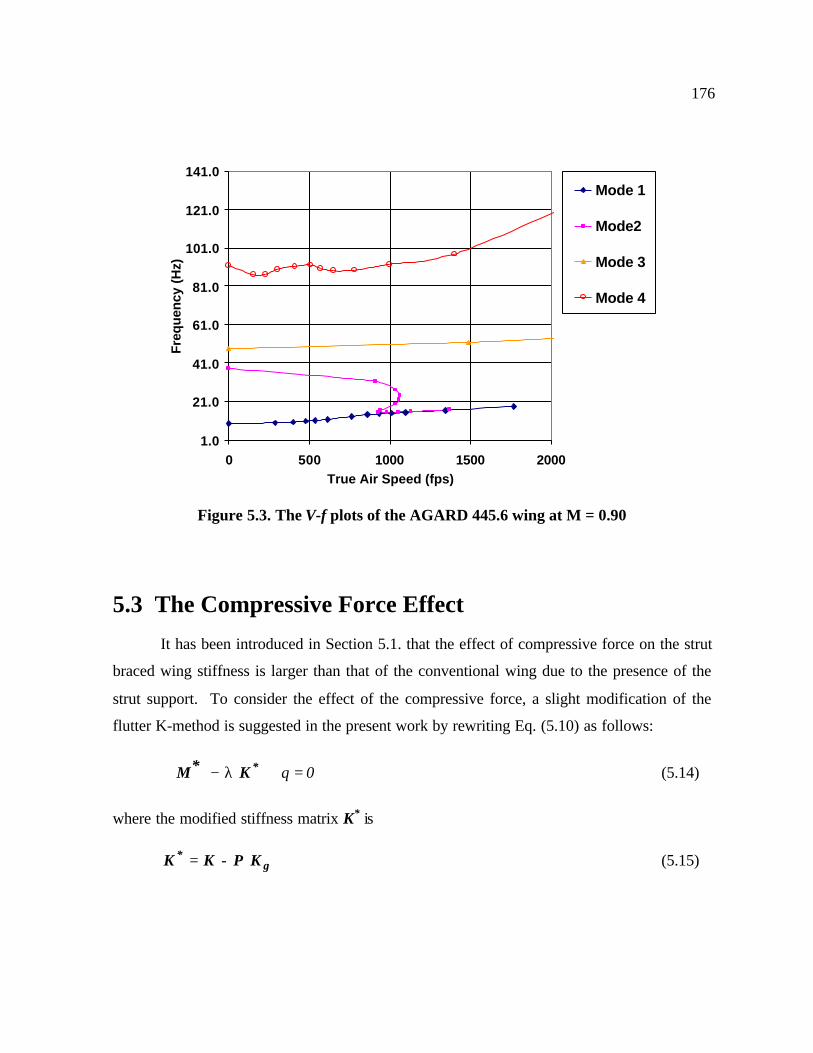
176
1.0
21.0
41.0
61.0
81.0
101.0
121.0
141.0
0 500 1000 1500 2000True Air Speed (fps)
Freq
uenc
y (H
z)Mode 1
Mode2
Mode 3
Mode 4
Figure 5.3. The V-f plots of the AGARD 445.6 wing at M = 0.90
5.3 The Compressive Force Effect
It has been introduced in Section 5.1. that the effect of compressive force on the strut
braced wing stiffness is larger than that of the conventional wing due to the presence of the
strut support. To consider the effect of the compressive force, a slight modification of the
flutter K-method is suggested in the present work by rewriting Eq. (5.10) as follows:
0q =
λ− *K*M (5.14)
where the modified stiffness matrix K* is
g* KP-KK = (5.15)

177
and Kg and P are the geometric stiffness matrix and the internal force and moment of the
structure, respectively. For the present flutter calculation, the internal force P is calculated
from the force equilibrium of the wing-strut structure at 1.0 g cruise flight condition. This
internal force P is used also in the calculation of the natural frequencies and mode shapes of
the wing-strut structure.
Therefore, the flutter speed procedure adopted in the present work is as follow:
1. Find the wing and strut stiffness and mass distribution by using ehexa.f code described in
Chapter 2. The input data necessary for the code is the wing thickness distribution given
by the wing.f of the double plate model described in detail in Ref. 12..
2. Perform a trim analysis of the strut-braced wing at 1.0 g cruise flight condition to obtain
the internal force P. The wing flexibility and aerodynamic load redistribution is taken
into account in the analysis. The strut slack mechanism is also considered in the analysis,
i.e. the strut starts to engage when the load factor ns = 0.8 g in the present case.
3. Perform a modal analysis of the strut braced wing by including the effect of the
compressive force.
4. Calculate the generalized unsteady aerodynamics force based on the present doublet
lattice method. The mode shapes to generalize the aerodynamic matrix are taken from
the result of Step 2.
5. Calculate the flutter speed using the K-method. The stiffness matrix is modified by
including the compressive force effect. The generalized mass and aerodynamic force
matrices are taken from Steps 2 and 3 that has already taken into account the effect of the
compressive force.
Figure 5.4 shows the flow chart of the present flutter analysis procedure. A more detailed
description of Steps 1 and 2 are given in the next two sections.

178
wing.f ehexa.f fem.f
dlm . f flutter . f mode.f
EI, GJ, EAt/c
K - P Kg
f, Φ[A(k)]
Vf , ωf
trim.fvlm.f
K, Kg
[A]
Figure 5.4. Flowchart for the flutter analysis of the strut braced wing
5.4 Trim Analysis Of The Strut Braced Wing
The present trim analysis procedure is applied to the strut-braced wing aircraft with
fuselage-mounted engine. The aircraft configuration is obtained from an MDO code
developed at Virginia Tech described in Refs. 9 and 10. The MDO code includes influence
from several fields including aerodynamics, structures, performance, weights, and stability
and control. The aircraft take-off gross weight TOGW is minimized with the design
optimization package DOT.174 For the present strut-braced wing aircraft optimization, 19
design variables of the aircraft parameters including the location of the wing-strut junction ys

179
and strut force load Ps (Figs. 2.2 and 2.3) are used. The aircraft configuration data after final
MDO design are summarized in Table 5.2
Table 5.2. Strut-braced wing aircraft parameters
Wing half-span 108.44 ft
Wing - strut junction point 74.52 ft
Wing sweep (3/4 chord) 25.98°
Strut sweep (3/4 chord) 19.01°
Strut offset length 2.74 ft
Wing root chord 32.31 ft
Wing tip chord 6.77 ft
Strut force at 1 g load 215 387 lb
Strut chord (constant) 6.62 ft
Wing root t/c 13.75%
Wing tip t/c 6.44%
Strut t/c 8.0%
Fuselage diameter 20.33 ft
Wing flap area 1411.02 ft2
Wing reference area 4237.30 ft2
Take-off gross weight 504833 lb
For calculating the wing weight in the SBW optimization, a hexagonal wing-box
model representing the wing sections parameters including wing skin, spar caps, spar webs
and stringer is used (Fig. 2.4). This model is provided by Lockheed Martin Aeronautical
Systems (LMAS) in Marietta, Georgia.22 Based upon LMAS experience in wing sizing, the
wing-box geometry varies in the spanwise direction with optimized area and thickness ratios

180
for each of the wing section parameters. The bending and torsional stiffness of each wing
section computed based on this model is used further for flexible wing aeroelastic stability
analysis.
Several load cases are used to determine the SBW wing structural weight in the
optimization including 2.5 g pull-up maneuver, -1.0 g pushover and –2.0 g taxi bump. To
avoid strut buckling, a telescoping sleeve mechanism proposed by Virginia Tech for the
SBW design disengages strut during the negative-g maneuvers. For a positive-g maneuver
the strut first engages in tension at some positive load factor ng by providing a slack in the
wing-strut mechanism. If we define a slack load factor (SLF) as the load factor at which the
strut initially engages, the wing performs as a cantilever beam for ng < SLF and performs as
a strut-braced beam for ng > SLF. To prevent the strut from engaging and disengaging
during cruise due to gust loads, the slack load factor used in the present SBW configuration is
set to 0.8 during the optimization.
If the wing deformation and aerodynamic load redistribution are used to investigate
passive load alleviation due to aeroelastic effects, the present procedure includes additional
terms related to aerodynamic loading in the governing equation as follows:
[ ]{ } [ ] { } { }0xAqxKxPK g =+− )( (5.16)
where A is aerodynamic influence coefficient (AIC) matrix. In the present case, AIC is
calculated based on the vortex lattice method (VLM). A more detailed description of the
VLM procedure is described in Chapter 4.
Equation (5.16) shows that the axial force P is a function of the deformation x since
the wing-strut structure is statically indeterminate. However, the axial force is related also to
the wing-strut mechanism adopted in the present work. For a negative-g maneuver the strut
is disengaged to avoid strut buckling. For a positive-g maneuver the strut would first engage
at a load factor ng equals to the slack load factor, SLF, by providing a slack in the wing-strut
mechanism. Therefore two different structure configurations should be considered in order
to accurately calculate the wing deformation. The first configuration is the wing when the

181
strut is disengaged for ng < SLF where in this case P = 0 in Eq. (5.16). The second
configuration is the wing when the strut is engaged for ng > SLF where the geometric
stiffness of the wing and strut is used in the calculation. The stress-strain relationship for the
strut material is therefore idealized as shown in Fig. 5.5 where the strain εs is related to the
condition ng = SLF.
ε
σ
εs
Figure 5.5. A bilinear stress-strain relationship of the strut for calculation of wing responseunder aerodynamic loading. The strain εs is related to the strut slack load factor.
Another important aspect related to the solution of Eq. (5.16) is the fact that the
problem involves two different eigenvalues, namely the structural buckling load P and the
aeroelastic divergence speed q∞. To ensure the continuity from the first to the second
configurations of the wing deformation described previously, Eq. (5.16) is solved as a
boundary value problem, where P and q∞ are updated for each iteration as shown
schematically in Fig. 5.6. In the present work, q∞ is given as the dynamic pressure related to
the design cruise speed Vc, and the aircraft incidence is adjusted such that total lift is the same
as the take-off gross weight (TOGW) of the aircraft for each iteration.

182
Stiffness K
GeometricStiffness Kg
Aerodynamic Load A(x)
Deformation x
Internal Force Pi (x)
K - P i Kg
Bilinear Stress-Strain Relationship
Figure 5.6. Flow chart for the trim analysis of the SBW wing under aerodynamic loads
5.5 Modal Analysis
Based on the present finite element code mode.f, a structural dynamic analysis was
performed to calculate the natural frequencies and modes of the strut-braced wing. For all
the cases considered in the present work, the connection between the fuselage and wing strut
and between the fuselage and strut are assumed to be rigid, i.e there are no relative
displacements and rotations at the wing-fuselage and strut-fuselage junctions. The free-
vibration analysis was performed to the half wing model using the LAPACK eigen solver169.
The natural frequencies and mode shapes for the first seven modes are presented in Table 5.3
and Fig. 5.7. Table 5.3 also shows comparison between the results of the detailed wing
model used in Chapter 2 and the simplified wing beam model used in the present chapter.
The results show that the frequencies of the simplified beam model are close to the associated

183
frequencies of the detailed model. This simplified beam model is used further in the present
chapter for calculating the flutter speed.
Table 5.3.
Natural frequencies of the strut-braced wing
i Mode Shape
Simplified Wing
Beam Model
(Present Chapter)
f (Hz)
Detailed Wing
Model
(Chapter 2)
f (Hz)
1 First vertical bending 2.233 2.332
2 Second vertical bending 3.073 2.971
3 First aft bending 3.720 3.742
4 Third vertical bending 4.784 4.371
5 Fourth vertical bending 6.656 6.765
6 Fith vertical bending 8.538 7.708
7 First torsion 9.170 9.091

184
Y
X
Z
Fig 5.7a. Mode 1 ( 2.23 Hz)
Y
X
Z
Fig 5.7b. Mode 2 ( 3.07 Hz)
Y
X
Z
Fig 5.7c. Mode 3 ( 3.72 Hz)

185
Y
X
Z
Fig 5.7d. Mode 4 ( 4.78 Hz)
Y
X
Z
Fig 5.7e. Mode 5 ( 6.65 Hz)
Y
X
Z
Fig 5.7f. Mode 6 ( 8.54 Hz)

186
Y
X
Z
Fig 5.7g. Mode 7 ( 9.17 Hz)
5.6 Flutter Calculation at Reference Condition
In the present work, the flutter speed is calculated first for the reference condition,
and then followed by the flutter calculation for a number of parameter variations including
strut locations and flight altitudes. The reference condition for the present flutter calculation
is defined as follows:
• The wing and strut structural data are based on the final iteration result of the MDO study
• The wing strut junction location is at y = 0.69 of the wing half span.
• The computations are performed for sea level condition.
• Zero fuel distribution in the wing.
• The compressive force effect is fully included.
In the present flutter analysis, all of the first ten vibration modes are used and the
structural damping is assumed to be equal to 0%. The V-g and V-f plots of the flutter results
for the reference condition are shown in Figure 5.8. The flutter speed is found at Vf = 843.6
fps with the flutter frequency of f = 3.859 Hz. No divergence speeds was found for the
reference condition.

187
Comparison is also made to other methods as shown in Table 5.4. The first row is the
present flutter speed and frequency for a simplified beam model using the present doublet
lattice method. The second row is the results for the detailed wing-strut model with ZONA6
of ZAERO is used for the unsteady aerodynamic method and the g-method of ZAERO is
used for the flutter solution. Note that the g-method is a generalized PK method which is
more robust than the K-method. ZONA6 is derived based on a constant pressure method,
which is more accurate than the doublet lattice method.81 The constant pressure method uses
an assumption that the acceleration potential is distributed with a constant strength on the
surface of each element. The doublet lattice method uses a more restricted assumption, i.e. it
assumes that the acceleration potential is lumped with a constant strength on a line of each
element.81
The third row is the result for the detailed SBW model taken from Section 2.4. of the
present work. It was calculated using the PK method of NASTRAN. No compressive force
effect was included in the calculation for the detailed SBW model. Finally, the last row is the
Lockheed Martin calculation result for their detailed SBW model which is slightly different
than the present SBW model. Their wing final model has an anhedral angle. Their strut is
rigidly connected to the fuselage and wing, i.e. no strut slack mechanism is used. Their offset
beam is modeled as a curve beam. Comparing to these results, the present flutter procedure
for the simplified beam model gives a conservative result, i.e. the lowest flutter speed among
others. However, it will be shown in the next section that this flutter speed is still beyond the
flight speed envelope of the strut-braced wing design.

188
Table 5.4. Comparison of the flutter speed and frequency
of the strut braced wing
MethodStructure
ModelFlutter Solver
Flutter Speed(fps)
Flutterfrequency
(Hz)
Present DLM Beam model K-method 834.6 3.859
ZONA6 Detailed model* g-method 873.2 3.109
NASTRAN Detailed model* PK-method 902.0 3.93
LMAS Detailed model* N/A 1005 N/A
*) No compressive force effect

189
-0.5
-0.4
-0.3
-0.2
-0.1
0.0
0.1
0.2
0.3
0.4
0.5
0 500 1000 1500 2000True Air Speed (fps)
Dam
ping
Coe
ffic
ient
g
Mode 1
Mode2
Mode 3
Mode 4
Mode 5
Mode 6
Mode 7
Mode 8
Mode 9
Mode 10
1.0
3.0
5.0
7.0
9.0
11.0
13.0
15.0
0 200 400 600 800 1000True Air Speed (fps)
Fre
qu
ency
(H
z)
Mode 1
Mode2
Mode 3
Mode 4
Mode 5
Mode 6
Mode 7
Mode 8
Mode 9
Mode 10
Figure 5.8. The V-g and V-f plots of the strut braced wing at the reference condition

190
5.7. Sensitivity Analysis
A sensitivity study was performed to study the behavior of the aeroelastic response
near the reference condition described in the previous section. Variation of several
parameters are selected including the changes of:
• spanwise position of the wing-strut junction
• offset beam length in the wing-strut junction
• altitude
It is assumed that the stiffness and dimension of the wing and strut are fixed at the
reference condition as the aforementioned parameters are made to vary.
The first variation is to investigate the variation of the flutter speed if the wing-strut
junction position changes along the spanwise direction. Two different flutter results for the
strut braced wing are shown in Figure 5.9. The first result, shown in Fig. 5.9 by a line with
triangular symbols, is for the strut braced wing but ignoring the compressive force effect, i.e.
the wing strut is statically indeterminate but the stiffness matrix of the system is not modified
by the P Kg term. The second result, shown by a line with rectangular symbols, is for the
same strut-braced wing but with the compressive effect included. Comparison between these
two results are important to investigate the trend of the compressive force along the spanwise
direction. Several conclusion that can be drawn from the results are as follow:
• The compressive force tends to give a lower flutter speed. Figure 5.9 shows that the
second plot, the one with compressive effect, is almost always below the first plot.
• The influence of the compressive force is not significant if the wing-strut junction is near
the wing root. Figure 5.9 shows that if the wing-strut location ys is less than 0.3 than the
two plots are identical, i.e. we can ignore the influence of the compressive force for this
case.

191
• The influence of the compressive force is significant if the wing strut junction is placed
near the wing tip. Figure 5.9 shows that for ys > 0.8, the flutter speed of the second plot
drops faster than the first plot.
• The flutter speed is reduced significantly when the wing-strut junction is moved toward
the wing tip from ys = 0.5 to 1.0. Note that, for the second plot, the flutter speed at ys =
1.0 is almost one third of the flutter speed at ys = 0.5. This trend is related to the decrease
of the strut stiffness as its length increases. The strut cross sectional area and moment of
inertia are kept constant in this sensitivity study.
• Note that the second plot has a dip near ys = 0.4. The reduction of the flutter speed here is
related to the switch of the flutter mode from the bending mode to the torsion mode.
0
0.2
0.4
0.6
0.8
1
1.2
1.4
1.6
1.8
2
0 0.1 0.2 0.3 0.4 0.5 0.6 0.7 0.8 0.9 1
y / half span
Vfl
utt
er /
Vre
f
Wing-Strut with P [ Kg ] = 0
Wing-Strut with P [ Kg ] = 0
Figure 5.9. Flutter speed as a function of the spanwise position of the strut junction at
the wing. Vref = 834.6 fps.
y

192
The second sensitivity study is performed to investigate the variation of the flutter
speed if the length of the offset beam changes. Figure 5.10 shows the results for three
different spanwise location of the wing-strut junction, i.e at ys = 0.56, 0.69 and 1.0. Figure
5.10 indicates that the flutter speed decreases as the length of the offset beam increases. This
trend is the same for the three different spanwise locations of the wing strut junction. These
results are expected since the increase of the offset beam length will reduce the wing-strut
stiffness, and thus reduce the flutter speed. All of the calculations were performed by
including the effect of the compressive force.
0
0.2
0.4
0.6
0.8
1
1.2
1.4
1.6
1.8
0 1 2 3 4 5
Offset beam length hoffset / href
Vfl
utt
er /
Vre
f
Wing-Strut JunctionPosition: y / b = 0.56
y / b = 0.69
y / b = 1.0
Figure 5.10. Flutter speed as function of the length of the offset beam at the wing-strut
junction. Vref = 834.6 fps.
hoffset
y

193
Finally, the flutter speed was calculated for the wing with and without strut for every
altitude. Related to the FAA regulation,25 this condition is required to check the flutter speed
of an aircraft not only for a nominal/healthy condition but also for a failure condition. The
flutter speed for a nominal aircraft should be greater than 1.2 of VD, and for a failure
condition should be greater than VD, where VD is a dive speed which is greater than the
design cruise speed. A brief description of the aeroelastic stability envelope is given in
Appendix B.
Figure 5.11 presents the results and comparison with the flight envelope. The wing
without strut in the present case gives higher flutter speed than that of the wing with strut.
The lower flutter speed for the wing with strut is related to the effect of the compressive force
that reduces the stiffness of the inboard part of the wing. Aerodynamic interference between
the strut and wing may also contribute to the reduction of the flutter speed. This trend is
different than the flutter solution of the Keldysh problem given in Refs. 27 and 28 where the
flutter speed for the wing with strut is higher than the wing without strut. In the Keldysh
problem, the strut is assumed to have an infinite stiffness such that the wing does not move in
lateral directions at the wing-strut junction location. The effect of the strut compressive force
is also ignored in the Keldysh problem, i.e. the inner wing stiffness does not decrease.
Therefore, the structural stiffness for the wing with strut in the Keldysh problem is stronger
than the wing without strut, and thus the flutter speed is higher for the wing with strut than
the wing without strut.
Figure 5.11 also shows that the present design of the strut-braced wing aircraft is free
from flutter within its flight envelope. This important conclusion is in agreement with the
finding by LMAS in Ref. 26. The strut braced wing aircraft version of LMAS is derived
from the present configuration with a more refined aerodynamic and structural design of the
wing. After performing a flutter analysis using a more detailed aircraft structure, LMAS
concluded, in their final report to NASA-Langley, that their strut-braced wing is free from
flutter.

194
0
5
10
15
20
25
30
35
40
45
0 0.5 1 1.5 2 2.5Vflutter / Vref
Alt
itu
de
(k f
t)
Wing without Strut
Wing with Strut
LMAS Result
Figure 5.11. Flutter speed boundary of the strut braced wing. Vref = 834.6 fps.
Flutter Boundary

CHAPTER 6
Conclusions
The focus of the present work was to investigate the effect of compressive force on
aeroelastic stability analysis of a strut-braced wing by using efficient structural finite element
and aerodynamic lifting surface methods. The main goal is to develop an aeroelastic analysis
code that is accurate but fast enough to be implemented as a tool in a multidisciplinary
optimization environment.
A study to reduce the aeroelastic computational time has been conducted by reducing
the number of elements of wing structure and aerodynamic models. To minimize the number
of wing structural elements, an accurate finite element formulation for non-uniform beam is
developed. For a static problem, the present formulation yields an exact stiffness matrix of
the beam with arbitrary polynomial variation of the beam stiffness. For a buckling problem,
a new procedure was introduced to improve the accuracy by using a quadratically convergent
iteration technique. The results shows that the number of the beam element can be reduced
significantly without degrading the accuracy.
To minimize the number of aerodynamic panel models, an efficient unsteady
aerodynamic formulation for multiple lifting surfaces was developed. The present
formulation improves the accuracy of existing lifting surface methods by implementing a
more rigorous treatment of the aerodynamic kernel integration. The singularity of the kernel
function is identified and isolated by implementing an exact expansion series to solve a
modified cylindrical function problem. An exact integration is performed to the singular part

196
of the kernel. A Gaussian quadrature is used to integrate the regular part of the kernel that
allows to increase the accuracy of the integration without changing the formulation scheme.
A hybrid doublet lattice/doublet point scheme is devised to further reduce the total number of
integration points by increasing the integration points near a rapid variation of the kernel
function and reducing the integration points near a gradual variation of the kernel. Validation
has been performed to a number of wing planforms and the results are in good agreements
with those obtained using other methods.
In order to include the compressive force in the aeroelastic solution, a static
aeroelastic analysis procedure was developed to calculate the internal forces and moment of
the structural element during the 1.0 g cruise flight. The wing structural flexibility and the
compressive force effect are considered in the analysis. The strut is allowed to deform
following the bilinear stress-strain relationship to model the slack mechanism of the strut to
engage and disengage during the vehicle maneuver, including the 2.5 g and – 1.0 g load
maneuvers .
The flutter solution module combines all of the structural stiffness, inertia and
geometric stiffness matrices, the aerodynamic influence coefficient matrix, and the internal
compressive load data to perform aeroelastic stability analysis. The flutter K method is
selected as the flutter solver since it is one of the fastest among other techniques. Validation
of the procedure to a standard AGARD 445.6 wing at several Mach numbers shows that the
results are in good agreement with those of wind tunnel test and other methods, except for
Mach number near 1.0 where the nonlinear transonic flow effect should be taken into
account.
The aeroelastic procedure above has been implemented to investigate the influence of
the compressive force on the flutter speed of the strut-braced wing. The aircraft
configuration selected is the strut-braced wing aircraft with fuselage-mounted engine with the
technical data given in Table 5.1. Flutter analysis was performed to the final MDO design
and parametric studies with respect to several design studies were conducted to study the
effect of the compressive force. The flutter boundary was constructed based on the Federal

197
Aviation Regulation §25.629 and § 25.333. Several conclusions that can be drawn are as
follows:
• No flutter occurs within the flight envelope of the present strut-braced wing
configuration.
• The compressive force tends to decrease the flutter speed
• Flutter speed reduces as the following parameters changes:
− The wing-strut junction position moves outward toward the wing tip
− The wing strut junction position moves along chordwise direction from wing front
spar to rear spar.
− The length of the offset beam connecting the wing and strut increases
− The flight altitude decreases
• The best location of the wing-strut junction is located between 50% - 80% of the wing
half-span measured from the wing root. (Note that the location of the wing-strut junction
of the present design is at 69%).
• The compressive force effect is significant to decrease the inner wing buckling capacity
and the flutter speed if the wing-strut junction is placed near the wing tip.

CHAPTER 7
Future Work
Although this research represents the latest in a long line of work that has been
performed in an effort to investigate the advantage and disadvantage of the strut-braced wing
design, there is still much work to be done. Among topics that warrant further study in the
area presented in this research are as follows:
• The aeroelastic procedure in the present work was developed in a modular form that can
be applied to other wing designs by turning off the compressive force effect. However
more work is needed to improve the efficiency of the eigen solver code. Currently, the
eigen solver used is dsbgv.f of LAPACK where all eigenvalues of the generalized eigen
problem are computed. On the other hand only a few eigenvalues are needed for the
flutter analysis. In the present work, the order of the structural finite element equations
are between 400 to 500, but, typically, only the first ten modes are needed for wing flutter
analysis. One of possible best candidates to replace the current eigen solver is the sub-
space iteration technique described in Ref. 195.
• Static and dynamic aeroelastic stability analysis were investigated in the present work,
but no aeroelastic response analysis due to gust loads was performed. If the acceleration
amplitude of the wind gust oscillates beyond 1.0 g load, than it would be necessary to
include the geometrically non-linear analysis in the time domain aeroelastic simulation.
The present formulation for the unsteady aerodynamic was derived in Laplace domain,
therefore it is still suitable to be implemented for the transient type motion.

199
• The strut-braced wing configuration selected in the present work was the final design of
the SBW fuselage-mounted engine. A similar aeroelastic procedure can be performed to
other configurations including the SBW under-wing engine and the SBW tip-engine
configurations.
• The present study was based on a linear unsteady aerodynamic theory that may not be
accurate near sonic Mach number. Application of higher order aerodynamic prediction
would be necessary to capture the so-called transonic dip effect in aeroelastic stability
analysis.

References
1. Pfenninger, W., “Design Considerations of Large Subsonic Long Range Transport
Airplanes with Low Drag Boundary Layer Suction,” Northrop Aircraft, Inc., Report
NAI-54-800 (BLC-67), November 1954.
2. Jobe, C.E., Kulfan, R.M., and Vachal, J.D., “Wing Planforms for Large Military
Transports,” AIAA-78-1470, 1978.
3. Kulfan, R.M., and Vachal, J.D., "Wing Planform Geometry Effects on Large Subsonic
Military Transport Airplanes," Boeing Commercial Airplane Company, AFFDL-TR-
78-16, February 1978.
4. Park, H. P., "The Effect on Block Fuel Consumption of a Strutted vs. Cantilever Wing
for a Short Haul Transport Including Strut Aeroelastic Considerations," AIAA-78-
1454-CP, Los Angeles, California, Aug. 21-23, 1978.
5. Turriziani, R.V., Lovell, W.A., Martin, G.L., Price, J.E., Swanson, E.E., and Washburn,
G.F., "Preliminary Design Characteristics of a Subsonic Business Jet Concept
Employing an Aspect Ratio 25 Strut Braced Wing," NASA CR-159361, October 1980.
6. Smith, P.M., DeYoung, J., Lovell, W.A., Price, J.E., and Washburn, G.F., “A Study of
High-Altitude Manned Research Aircraft Employing Strut-Braced Wings of High-
Aspect Ratio,” NASA CR-159262, February, 1981.
7. Grasmeyer, J.M., Naghshineh-Pour, A.H., Tetrault, P.A., Grossman, B., Haftka, R.T.,
Kapania, R.K., Mason, and W.H., Schetz, "Multidisciplinary Design Optimization of a

201
Strut-Braced Wing Aircraft with Tip-Mounted Engines," MAD Center Report 98-01-
01, Virginia Tech, January 1998.
8. Grasmeyer, J.M., “Multidisciplinary Design Optimization of a Strut-Braced Wing
Aircraft,” MS Thesis, Virginia Tech, April 1998.
9. Gern, F.H., Ko, A., Sulaeman, E., Gundlach, J.F., Kapania, R.K., and Haftka, R.T.,
“Multidisciplinary Design Optimization of a Transonic Commercial Transport with a
Strut-Braced Wing,” Journal of Aircraft, Vol. 38, No. 6, 2001, pp. 1006-1014.
10. Gundlach, J.F., Gern, F.H., Tetrault, P, Naghshineh-Pour, A.H., Ko, A., Schetz, J.A.,
Mason, W.H., Grossman, B., Kapania, R.K., and Haftka, R.T., “Multidisciplinary
Design Optimization of a Strut-Braced Wing Transonic Transport,” AIAA Paper 2000-
0420, Jan. 2000.
11. Tretault, P.A., “Numerical Prediction of the Interference Drag of a streamlined Strut
Intersecting a Surface in Transonic Flow,” Ph.D Dissertation, Virginia Tech, January
2000.
12. Tretault, P.A. , Schetz, J.A., and Grossman, B., “Numerical Prediction of Interference
Drag of Strut-Surface Intersection in Transonic Flow,” AIAA Journal, Vol. 39, No. 5,
May 2001, pp. 857-864.
13. Naghshineh-Pour, A.H.,” Structural Optimization and Design of a Strut-Braced Wing
Aircraft,” MS Thesis, Virginia Tech, November 1998.
14. Grossman, B., Strauch, G.J., Eppard, W.M., Gurdal, Z., and Haftka, R.T., "Integrated
Aerodynamic/Structural Design of a Sailplane Wing," AIAA-86-2623, Dayton, Ohio,
October 20-22, 1986.
15. Giunta, A.A., Balabanov, V., Haim, D., Grossman, B., Mason, W.H., Watson, L.T., and
Haftka, R.T., "Multidisciplinary Optimization of a Supersonic Transport Using Design
of Experiments Theory and Response Surface Modeling," The Aeronautical Journal,
pp. 347-356, October 1997.

202
16. Hutchison, M.G., Unger, E.R., Mason, W.H., Grossman, B., Haftka, R.T., "Variable
Complexity Aerodynamic Optimization of a High Speed Civil Transport Wing,"
Journal of Aircraft, Vol. 31, No. 1, pp. 110-116, 1994.
17. Ko, Y.A.,” The Role of Constraints and Vehicle Concepts in Transport Design: A
Comparison of Cantilever and Strut-Braced Wing Airplane Concepts,” MS Thesis,
Virginia Tech, April 2000.
18. Ko, Y.A., Grossman, B., Mason, W.H., and Haftka, R.T., ”The Role of Constraints in
the MDO of a Cantilever and Strut-Braced Wing Transonic Commercial Transport
Aircraft, AIAA Paper 2000-5609, SAE Paper 2000-01-5609, World Aviation
Conference, San Diego, CA, Oct. 10-12, 2000.
19. Gern, F.H., Sulaeman, E., Naghshineh-Pour, A., Kapania, R.K., and Haftka, R.T.,
“Flexible Wing Model for Structural Wing Sizing and Multidisciplinary Design
Optimization of a Strut-Braced Wing,” AIAA Paper 2000-1427, 41st
AIAA/ASME/ASCE/AHS/ASC Structures, Structural Dynamics, and Materials
Conference and Exhibit, Atlanta, GA, April 3-6, 2000.
20. Gern, F.H., Ko, A., Sulaeman, E., Kapania, R.K., Mason, W.H., Grossman, B., and
Haftka, R.T., “Passive load alleviation in the design of a strut-braced wing transonic
transport aircraft,” AIAA Paper 2000-4826, 8th AIAA/USAF/NASA/ISSMO Symposium
on Multidisciplinary Analysis and Optimization, Long Beach, CA, Sept. 6-8, 2000.
21. Gern, F.H., Naghshineh-Pour, A., Sulaeman, E., Kapania, R.K., and Haftka, R.T.,
“Structural Wing Sizing for Multidisciplinary Design Optimization of a Strut-Braced
Wing,” Journal of Aircraft, Vol. 38, No. 1, 2001.
22. Sulaeman, E., Kapania, R.K., and Haftka, R.T, “Effect of Compressive Force on a
Strut-Braced Wing Response,” AIAA Paper 2001-1611, 42nd AIAA/ASME/ASCE/AHS/
ASC Structures, Structural Dynamics, and Materials Conference and Exhibit, Seatle,
WA, April 16-19, 2001.
23. McCullers, L.A., FLOPS User’s Guide, Release 5.81, NASA Langley Research Center.

203
24. Kroo, I., Gallman, J.W., and Smith, S.C., “Aerodynamic and Structural Studies of
Joined-Wing Aircraft”, Journal of Aircraft, Vol. 28, No.1, 1991, pp. 74-81.
25. Miura, H., Shyu, A., and Wolkovitch, J., “Parametric Weight Evaluation of Joined
Wings by Structural Optimization”, Journal of Aircraft, Vol. 25, No. 12, 1988, pp.
1142-1149.
26. Oliffe, B., Private Communications with R.K. Kapania, May - June 1998.
27. Mailybaev, A.A., and Seiranyan, A.P. “The Keldysh Problem on Aeroelastic Stability
of a Strut-braced Wing,” Physics-Doklady, Vol. 41, No. 10, 1996, pp. 484-487
(Translated from original Russian text in Doklady Akademii Nauk , Vol. 350, No.4,
1996).
28. Keldysh, M.V., Izbrannye trudy: Mekanika, Moscow, Nauca, 1985, pp. 304 – 341.
29. Gern, F.H., Weekly Presentation of the Strut Braced Wing, MAD Center, AOE
Department, Virginia Tech, 1998 – 2000.
30. Anon., “Structural and Aerodynamic Investigation of a Strut-Braced Wing Transport
Aircraft”, Lockheed Martin Aeronautical Systems Phase 2 Final Report, Dec. 8, 1999.
31. de Lagrange, J.L., “Sur la Figure des Colonnes,” Miscellanea Taurinesia, Vol. 5, 1770-
1773, p. 173.
32. Taylor, J.E., and Liu, C.Y., “Optimal Design of Columns,” AIAA Journal, Vol. 6, No.
8, 1968, pp. 1497-1502.
33. Bisplinghoff, R.L., Ashley, H., and Halfman, R.L., Aeroelasticity, Addison-Wesley,
1955.
34. Rodden,W.P., and Johnson, E.H., MSC/NASTRAN Aeroelastic Analysis User’s Manual,
Version 68, 1994, pp. 237-257.
35. Heard,W.L., Bush, H.G., Wallsom, R.E., and Jensen, J.K., “A mobile work station
concept for mechanically aided astronaut assembly of large space trusses,” NASA
Technical Paper 2108, 1983, pp. 1-35.

204
36. Banerjee, J.R., and Williams, F.W., “Exact Bernoulli-Euler Static Stiffness Matrix for a
Range of Tapered Beam-Columns,” International Journal for Numerical Methods in
Engineering,” Vol. 23, 1986, pp. 1615-1628.
37. Weaver, W., and Gere, J.M., Matrix Analysis of Framed Structures, 3rd ed., Van
Nostrand Reinhold, New York, 1990.
38. Yang, T.Y., Finite Element Structural Analysis, Prentice Hall, 1986.
39. Lee, S.Y., Ke, H.Y., and Kuo, Y.H., “Exact Static Deflections of a Non-Uniform
Bernoulli-Euler Beam with General Elastic End Strains, “ Computers and Structures,
Vol. 36, No. 1, 1990, pp. 91-97.
40. Friedman, Z., and Kosmatka, J.B., “Exact Stiffness Matrix of a Non-Uniform Beam”,
Computers and Structures, Vol. 42, 1992, pp. 671-682.
41. Baker, G., “Exact Deflections in Non-prismatic Members,” Computer and Structures,
Vol. 61, No. 3, 1996, pp. 515-528.
42. Baker, G.,”A Numerical Parametric Study of Nonlinear Behavior in Variable Depth
Beams,” Ph.D. Dissertation, Heriot-Watt University, Edinburgh, 1987.
43. Lamb, R.S., “Stress Distributions in Tapered Concrete Beams,” Ph.D. Dissertation,
University of Nottingham, 1971.
44. Eisenberger, M., “An Exact Element Methods”, International Journal for Numerical
Methods in Engineering,” Vol. 30, No. 2, 1990, pp. 363-370.
45. Eisenberger, M., “Explicit Stiffness Matrices for Non-prismatic Members”, Computers
and Structures, Vol. 20, 1985, pp. 715-720.
46. Karabalis, D.L., and Beskos, D.E., “Static, Dynamic and Stability Analysis of
Structures Composed of Tapered Beams,” Computers and Structures, Vol. 16, No. 6,
1983, pp. 731-748.
47. Iremonger, M.J., ”Finite Difference Buckling Analysis of Non-Uniform Columns,”
Computers and Structures, Vol. 12, 1980, pp. 741-748.

205
48. Gallagher, R.H., and Lee, C.H., “Matrix Dynamic and Instability Analysis with Non-
uniform Elements”, International Journal for Numerical Methods in Engineering,” Vol.
20, No. 2, 1970.
49. Dube, G.P. and Dumir, P.C., ”Tapered Thin Open Section Beams on Elastic
Foundation-I. Buckling Analysis,” Computers and Structures, Vol. 61, 1996, pp. 845-
857.
50. Rajasekaran, S., “Instability of Tapered Thin Walled Beams of Generic Section,” J.
Engineering Mechanics, Vol. 120, 1994, pp. 1630-1640.
51. Bisplinghoff, R.L., Ashley, H., and Halfman, R.L., Aeroelasticity, Addison-Wesley,
1955.
52. Landahl, M.T., and Stark, V.J.E., “Numerical Lifting Surface Theory – Problems and
Progress,” AIAA Journal, Vol. 6, No. 11, Nov. 1968, pp. 2049 – 2000.
53. Rodden, W.P., Harder, R.L., and Bellinger, E.D., “Aeroelastic Addition to
NASTRAN,” NASA CR 3094, March 1979.
54. Dowell, E.H., Curtiss, H.C.Jr., Scanlan, R.H., Sisto, F., A Modern Course in
Aeroelasticity, 2nd ed., Kluwer Academic Pub., 1989.
55. Ashley, H., Widnall, S.E., and Landahl, M.T., “New Directions in Lifting Surface
Theory,” AIAA Journal, Vol. 3, No. 1, Jan . 1965, pp. 3 – 16.
56. Ashley, H., and Rodden, W.P., “Wing – Body Aerodynamic Interaction,” Annual
Review of Fluid Mechanics, Vol. 4, 1972, pp. 431 – 472.
57. Bisplinghoff, R.L., and Ashley, H., Principles of Aeroelasticity, Dover Pub., New York,
1962.
58. Rodden, W.P., “A Comparison of Methods Used in Interfering Lifting Surface Theory,
“AGARD R. 643., Feb. 1976.
59. Hildebrand, F.B., Advanced Calculus for Applications, 3rd ed., Prentice Hall, Tokyo,
1963.

206
60. Watkins, C.E., Runyan, H.L., and Woolston, D.S., “On the Kernel Function of the
Integral Equation Relating the Lift and Downwash Distribution of Oscillating Finite
Wings in Subsonic Flow, “ NACA Rept. 1234, 1955.
61. Kussner, H.G., “General Airfoil Theory,” NACA TM 979, 1941.
62. Giesing, J.P., Kalaman, T.P., and Rodden, W.P., “Subsonic Unsteady Aerodynamic for
General Configurations,” AFFDL-TR 71-5, 1971.
63. Yates, E.C., Jr., “ A Kernel Function for Nonplanar Oscillating Surfaces in Subsonic
Flow, “ AIAA Journal, Vol. 5, No. 4, Aug. 1966, pp. 1486-1488.
64. Landahl, M.T., “Kernel Function for Nonplanar Oscillating Surfaces in a Subsonic
Flow,” AIAA Journal, Vol. 4, No. 4, May 1967, pp. 1045-1046.
65. Laschka, B., “Das Potential und das Geschwindigkeitsfeld der Harmonisch schwin-
genden tragenden Flache bei Unterschallanstromung,” Z. Angew. Math. Mech., Vol. 43,
1963, pp. 325-333.
66. Ueda, T., and Dowell, E.H., “A New Subsonic Method for Lifting Surfaces in Subsonic
Flow,” AIAA Journal, Vol. 20, No. 3, March 1982, pp. 348 – 355.; Technical Comment
by Rodden, W.P., Vol. 22, No.1, p. 160.; Reply by Ueda, T. and Dowell, E.H., Vol. 22,
No.4, p.575.
67. Rodden, W.P., Giesing., J.P., and Kalman, T.P., “New Developments and Applications
of the Subsonic Doublet Lattice Method for Nonplanar Configurations,” Symposium on
Unsteady Aerodynamics for Aeroelastic Analyses of Interfering Surfaces, AGARD CP
90-71, April 1971.
68. Jones, R.T., and Cohn, D., “High Speed Wing Theory,” General Theory of High Speed
Aerodynamics, Vol. VI, Sec. A., Princeton Univ. Press., New Jersey, 1954.
69. DeYoung, J.(ed.), “Vortex Lattice Utilization,” NASA SP-405, 1976.
70. Albano, E. and Rodden, W.P., “A Doublet Lattice Method for Calculating Lift
Distribution on Oscillating Surfaces in Subsonic Flow,” AIAA Journal, Vol 7, No. 2,
Feb. 1969, pp. 279-285; Errata, AIAA Journal, Vol. 7, No. 11, Nov. 1969, p. 2192.

207
71. Jordan, P.F., ‘Reliable Lifting Surface Solutions for Unsteady Flow,” Journal of
Aircraft, Vol. 15, Sept. 1978, pp. 626-633.
72. Rodden, W.P., Giesing, J.P., and Kalman, T.P., “Refinement of the Nonplanar Aspects
of the Subsonic Doublet Lattice Lifting Surface Method,” Journal of Aircraft, Vol. 9,
Jan 1972, pp. 69 – 73.
73. Houbolt, J.C., “Some New Concepts in Oscillatory Lifting Surface Theory, “ AFFDL-
TR-68-2, 1969.
74. Ichikawa, I., “Doublet Strip Method for Oscillating Swept Tapered wings in
Incompressible Flow,” Journal of Aircraft, Vol. 22, No. 11, Nov. 1985, pp. 1008 –
1012.
75. Eversman, W., and Pitt, D.M., “Hybrid Doublet Lattice/Doublet Point Method for
Lifting Surfaces in Subsonic Flow, “ Journal of Aircraft, Vol. 28, No. 9, Sept. 1991, pp.
572 – 578.
76. Kalman, T.P., Rodden, W.P., and Giesing, J.P., “Application of the Doublet Lattice
Method to Nonplanar Configurations in Subsonic Flow,” Journal of Aircraft, Vol. 8,
No. 6, June 1971, pp. 406 – 413.
77. Ueda, T., “Asymptotic Expansion of the Kernel Function in Subsonic Unsteady Lifting
Surface Theory,” Journal of the Japan Society for Aeronautical Space Sciences, Vol 20,
No. 326, 1981, pp. 169 – 174.
78. Ueda, t., “Expansion Series of Integral Functions in Unsteady Aerodynamics,” Journal
of Aircraft, Vol. 19, No. 7, April 1982, pp. 345 – 347.
79. Bismarck – Nasr, M.N., “Kernel Function Occuring in Subsonic Unsteady Potential
Flow,” AIAA Journal, Vol 29, No. 6, June 1991, pp. 878 – 879.
80. Rodden, W.P., MSC NASTRAN Handbook for Aeroelastic Analysis, Rept. MSR-57, The
MacNeal-Schwendler Corp., Los Angeles, Nov. 1987.
81. Mook, D.T. and Nayfeh, A.H., “Application of the Vortex Lattice Method to High
Angle of Attack Subsonic Aerodynamics,” SAE Paper No. 851817, Oct. 1985.

208
82. Ando, S. and Ichikawa, A., “Quadratic Formulas for Chordwise Integrals of Lifting
Surface Theories,” AIAA Journal, Vol. 21, No. 3, March 1983.
83. Stark, V.J.E., “A Generalized Quadrature Formula for Cauchy Integrals,” AIAA
Journal, Vol. 9, No. 9, Sept. 1971, pp. 1854 – 1855.
84. Bera, R.K., “Quadrature Formula for a Double Pole Singular Integral, AIAA Journal,
Vol. 26, No.6, June 1988.
85. Song, C.C.S., “Numerical Integration of a Double Integral with Cauchy-Type
Singularity,” AIAA Journal, Vol. 7, No. 7, July 1960, pp. 1389 – 1390.
86. Brandao, M.P., “Improper Integrals in Theoretical Aerodynamics: The Problem
Revisited,” AIAA Journal, Vol. 25, No. 9, 1987, pp. 1258 – 1260.
87. Van Niekerk, B., “Integration of Singular Functions Associated with Lifting Surface
Theory,” AIAA Journal, Vol. 24, No. 7, July 1986, pp. 1194 – 1196.
88. Lan, C.E., “Some Applications of the Quasi-Vortex Lattice Method in Steady and
Unsteady Aerodynamics”, NASA SP-405, 1976, pp. 385 – 406.
89. Graham, J.M.R., “A Lifting Surface Theory for the Rectangular Wing in Non-
Stationary Flow,” Aeronautical Quarterly, Vol 12, Feb. 1971, p. 83.
90. Margason, R.J., and Lamar, J.E., “Vortex Lattice Fortran Program for Estimating
Subsonic Aerodynamic Characteristics of Complex Planform,” NASA TN D-6142, Feb.
1971.
91. Lottati, I., and Nissim, E., “Oscillatory Piecewise Continuous Kernel Function
Method,“ Journal of Aircraft, Vol. 14, No. 6, June 1977, pp. 515 – 516.
92. Lottati, I., and Nissim, E., “Three-Dimensional Oscillatory Piecewise Continuous
Kernel Function Method. Part I, II and III,“ Journal of Aircraft, Vol. 18, No. 5, May
1981, pp. 346 - 363.
93. Lottati, I., and Nissim, E., “Nonplanar, Subsonic, Three-Dimensional Oscillatory
Piecewise Continuous Kernel Function Method,“ Journal of Aircraft, Vol. 22, No. 12,
Dec 1985, pp. 1043 - 1048.

209
94. Hough, G.R., “Remarks on Vortex Lattice Methods,” Journal of Aircraft, Vol. 10, No.
5, May 1973, pp. 314 – 317.
95. Hewitt, B.L., “Unsteady Airforces for wings with Control Surfaces,” Symposium on
Unsteady Aerodynamics for Aeroelastic Analyses of Interfering Surfaces, AGARD CP-
80-71, April 1971.
96. Rowe, W.S., Redman, M.C., Ehlers, F.E., and Sebastian, J.D., “Prediction of Unsteady
Aerodynamic Loading Caused by Leading Edge and Trailing Edge Control Surface
Motion in Subsonic Flows, NASA CR-2543, 1975.
97. Bohm, G., and Schmid, H., “Subsonic Unsteady Airloads on Multiple Lifting
Surfaces,“ Symposium on Unsteady Aerodynamics for Aeroelastic Analyses of
Interfering Surfaces, AGARD CP-80-71, April 1971.
98. Davies, D.E., “Calculation Methods for Unsteady Airforces of Tandem Surfaces and T-
Tails in Subsonic Flow,” Symposium on Unsteady Aerodynamics for Aeroelastic
Analyses of Interfering Surfaces, AGARD CP-80-71, April 1971.
99. Dat, R., and Akamatsu, Y., Representation d’Une Aile par des Lignes Portantes:
Application au Calcul de l’Interaction de Deux Ailes en Tandem,“ Symposium on
Unsteady Aerodynamics for Aeroelastic Analyses of Interfering Surfaces, AGARD CP-
80-71, April 1971.
100. Lan, C.E., “A Quasi Vortex Lattice Method in Thin Wing Theory,” Journal of Aircraft,
Vol. 11, No. 9, Sept. 1974, pp.518 – 527.
101. Watkins, C.E., Woolston, D.S., and Cunningham, H.J., “A Systematic Procedure for
determining Aerodynamic Forces on Oscillating or Steady Finite Wings at Subsonic
Speed,” NASA R-48, 1959.
102. Laschka, B., “Zur Theorie der Harmonisch Schwingenden Tragenden Flache bei
Unterschallanstromung,” Z. Flugwissenschaften, Vol. 11, No. 7, 1963, pp. 265 – 292.
103. Dat, R. and Malfois, J.P., “Sur le Calcul du Noyau de l’Equation Integrale de la Surface
Postante en Ecoulement Subsonique Instationnaire,” La Recherche Aerospatiale, No. 5,
1970, pp. 251 – 259.

210
104. Desmarais, R.N., “Accurate Numerical Evaluation of Modified Struve Functions
Occurring in Unsteady Aerodynamics,” Journal of Aircraft, Vol. 16, No. 7, July 1979,
pp. 441 - 447.
105. Berman, H.J., Shyprykevich, P., and Smedfjeld, J.B., “A Subsonic Nonplanar Kernel
Function for Surfaces Inclined to the Freestream,” Journal of Aircraft, Vol. 7, No. 2,
Feb. 1970, pp. 188 – 190.
106. Lance, G.N., “The Kernel Function of the Integral Equation Relating the Lift and
Downwash Distributions of Oscillating Finite Wings in Subsonic Flow,” Journal of
Aeronautical Sciences, Vol. , 1954, pp. 635 – 636.
107. Ando, S. and Kato, M., “Evaluation of the Desmarais’s Method Computing Subsonic
Kernel Function,” Journal of the Japan Aeronautical Space Sciences, Vol. 36, No. 418,
1988, pp. 529 – 534.
108. DeYoung, J., “Convergence-Proof of Discrete-Panel Wing Loading Theories,” Journal
of Aircraft, Vol. 8, No. 10, Oct. 1971, pp. 837 – 839.
109. Ward, G.N., Linearized Theory of Steady High Speed Flow, Cambridge Univ. Press.,
New York, 1955.
110. Bertin, J.J. and Smith, M.L., Aerodynamics for Engineers, Prentice-Hall, New Jersey,
1979.
111. Abramowitz, M., and Stegun, I.A. (eds.), Handbook of Mathematical Functions,
National Bureau of Standards, 1965.
112. Fogiel, M. (ed.), Handbook of Mathematical Scientific and Engineering Formulas,
Tables, Functions, Graphs, and Transforms, REA, New Jersey., 1991.
113. Prudnikov, A.P., Brychkov, Y.A., Marichev, O.I., Integrals and Series, Gordon and
Breach Science Pub., N.Y., 1986.
114. Allen, E.E., “Polynomial Approximations to Some Modified Bessel Functions,” Math.
Tables Aids Comp., Vol. 10, 1956, pp. 162 – 164.
115. Ghizzetti, A., and Oscini, A., Quadrature Formulae, Academic Press, New York, 1970.

211
116. Stroud, A.H., and Secrest, D., Gaussian Quadrature Formulas, Prentice Hall, New
York, 1983.
117. Katz, P., and Plotkin, A., Low-Speed Aerodynamics, McGraw-Hill, Inc., New York,
1991.
118. Singh, B.K., and Basu, B.C., “A Numerical Model for Analysis of Thin wings in
Inviscid Incompressible Flow,” Aeronautical Journal, Vol. 91, August-Sept. 1987, pp.
333 – 337.
119. Lamar, J.E., “A Modified Multhopp Approach for Predicting Lifting Pressures and
Camber Shape for Composite Planforms in Subsonic Flow,” NASA TN-D 427, July
1968.
120. Wagner, S., “On the Singularity Method of Subsonic Lifting Surface Method,” Journal
of Aircraft, Vol. 7, No. 6, 1969, pp. 549 – 558.
121. Thiel, A., Weissinger, J., “Pressure Distribution Measurement on a Straight and on a
350 Swept-Back Tapered Wings, NACA TM-1126, 1948.
122. Fischel, J., Naseth, R.L., Hagerman, J.R., O’Hara, W.M., “Effect of Aspect Ratio on the
Low Speed Lateral Control Characteristics of Untapered Low Aspect Ratio Wings
Equipped with Flap and with Retractable Ailerons,” NACA Rep. 1091, 1952.
123. Graham, R.R., “Low Speed Characteristics of a 450 Sweptback Wing of Aspect Ratio 8
from Pressure Distributions and Force Tests at Reynolds Numbers from 1,500,000 to
4,800,000,” NACA RM L51H13, 1951.
124. Wick, B.H., “Chordwise and Spanwise Loadings Measured at Low Speed on a
Triangular Wing Having an Aspect Ratio of Two and NACA 0012 Airfoil Section,”
NACA TN 1650, 1948.
125. Forsching, H., Triebstien, H., and Wagener, J., “Pressure Measurement on a
Harmonically Oscillating Swept Wing with Two Control Surfaces in Incompressible
Flow,“ Symposium on Unsteady Aerodynamics for Aeroelastic Analyses of Interfering
Surfaces, AGARD CP-80-71, April 1971.

212
126. DeJarnette, F.R., “Arrangement of Vortex Lattics on Subsonic Wings,” NASA SP 405,
1976, pp. 301 – 323.
127. Cunningham, A.M.,Jr., “An Efficient Steady, Subsonic, Collocation Method for
Solving Lifting Surface Problems,” Journal of Aircraft, Vol. 8, No. 3, Mar. 1971, pp.
168 – 192.
128. Hough, G.R., “Lattice Arrangements for Rapid Convergence,” NASA SP 405, 1976, pp.
325-342.
129. Rowe, W.S., and Cunningham, H.J., “On the Convergence of Unsteady Generalized
Aerodynamic Forces,” Journal of Aircraft, Vol. 21, No. 6, June 1984, pp. 420 – 427.
130. Harder, R.L., and Rodden, W.P., “Kernel Function for Nonplanar Oscillating Surfaces
in Supersonic Flow,” Journal of Aircraft, Vol. 8, No. 8, Aug. 1971, pp. 677 – 679.
131. Ueda, T. and Dowell, E.H., “Doublet Point Method for Supersonic Unsteady Lifting
Surfaces,” AIAA Journal, Vol. 20, No. 3, Mar. 1982, pp. 348 - 335.
132. Giesing, J.P., and Kalman, T.P., “Oscillatory Supersonic Lifting Surface Theoru using a
Finite element Doublet Representation,” AIAA Paper 75-761, May 1975.
133. Brock, B.J., and Griffin, J.A., Jr., “The Supersonic Doublet Lattice Method – A
Comparison of Two Approaches,” AIAA Paper 75-760, May 1975.
134. Ando, S., and Kato, M., “Evaluation of the Desmarais Method for Computing Subsonic
Kernel Function,” Journal of Japan Society for Aeronautical Space Sciences, Vol. 36,
No. 418, 1988, pp. 529 – 534.
135. Sulaeman, E., ”Discrete Element Methods for Calculating Aerodynamic Loadings on
Lifting Surfaces in Unsteady Subsonic Flows,” MS. Thesis, University of Dayton, Ohio,
1993.
136. Ueda, T., “Lifting Surface Calculations in the Laplace Domain with Application to
Root Loci,” AIAA Journal, Vol 25, No. 5, May 1987, pp. 698 – 704.
137. Hedman, S.G., “Vortex Lattice Method for Calculation of Quasi Steady State Loadings
on Thin Elastic Wings,” Aeronautical Research Institute of Sweden Rept. 105, Oct.
1965.

213
138. Blair, M., “A Compilation of the Mathematics Leading to the Doublet Lattice Method,”
WPAFB Air Force Wright Laboratory WL-TR-95-3022, November 1994.
139. Mason, W.H, Applied Computational Aerodynamics, Virginia Tech. AOE Class Note,
Blacksburg, 1999.
140. Belotserkovskii, S.M., The Theory of Thin Wings in Subsonic Flow, Plenum Press, New
York, 1967.
141. Falkner, V.M, “The Calculation of Aerodynamic Loading on Surfaces of any Shape,”
British Aeronautical Research Council R & M 1910, 1943.
142. Campbell, G.S., “A Finite Step Method for the Calculation of Span Loadings of
Unusual Plan Forms,” NACA RM L50L13, July 1951.
143. Rodden, W.P., Taylor, P.F., and McIntosh, S.C., Jr., “Further Refinement of the
Nonplanar Aspects of the Subsonic Doublet Lattice Lifting Surface Method,”
International Council of the Aeronautical Sciences (ICAS), Paper 96-2.8.2, 1996.
144. Rodden, W.P., Taylor, P.F., and McIntosh, S.C., Jr., “Further Refinement of the
Subsonic Doublet Lattice Method,” Journal of Aircraft, Vol. 35, No. 5, 1998, pp. 720–
727.
145. Rodden, W.P., Taylor, P.F., McIntosh, S.C., Jr., and Baker, M.L, “Further Convergence
Studies of the Enhanced Subsonic Doublet Lattice Oscillatory Lifting Surface Method,”
Proceedings of the International Forum on Aeroelasticity and Structural Dynamics,
Vol. III, Rome, Italy, 1997, pp. 401-408.
146. Van Zyl, L.H., “Arbitrary Accuracy Integration scheme for the Subsonic Doublet
Lattice Method,” Journal of Aircraft, Vol. 35, No. 6, pp. 975-977.
147. Van Zyl, L.H., “Convergence of the Subsonic Doublet Lattice Method,” Journal of
Aircraft, Vol. 35, No. 6, pp. 977-979.
148. Van Zyl, L.H., “Application of the Subsonic Doublet Lattice Method to Delta Wings,”
Journal of Aircraft, Vol. 36, No. 3, pp. 609-611.

214
149. Chen, P.C., Lee, H.W., and Liu, D.D., “Unsteady Subsonic Aerodynamics for Bodies
and Wings with External Stores including Wake Effect,” Journal of Aircraft, Vol. 30,
No. 5, Sept.-Oct. 1993, pp. 618 – 628.
150. Liu, D.D., Chen, P.C., Yao, Z.X., and Sarhaddi, D., “Recent Advances in Lifting
Surface Methods,” The Royal Aeronautical Journal, Vol. 100, No. 998, Oct. 1996, pp.
327 – 339.
151. Epstein, R.J., and Bliss, D.B., “Alternative Solution of the Kernel Function in Subsonic
Unsteady Lifting Surface Theory,” AIAA Journal, Vo. 33, No. 11, 1995, pp. 2228-2230.
152. Abrate, S., “Vibration of Non-Uniform Rods and Beams,” Journal of Sound and
Vibration, Vol. 185, No. 4, 1995, pp. 703-716.
153. Kumar, B.M., and Sujith, R.I., “Exact Solutions for Longitudinal Vibration of Non-
Uniform Rods, “ Journal of Sound and Vibration, Vol. 206, No. 5, 1997, pp. 721-729.
154. Eisenberger, M., “Exact Longitudinal Vibration Frequency of a Variable Cross-section
Rods”, Applied Acoustics, Vol. 34, No. 2, 1991, pp. 123-130.
155. Chehil, D.S., “Determination of Natural Frequencies of a Beam with Varying Section
Properties,” J. Sound and Vibration, Vol. 115, 1987, pp. 423-436.
156. Chen, Y.Z., and Xie, J.R., “ Evaluation of Natural Frequencies of Non-Uniform Beams
by Numerical Integration,” Computers and Structures, Vol. 29, 1988, pp. 693-697.
157. Plaut, R.H., Johnson, L.W. and Olhoff, N., “Bimodal Optimization of Compressed
Columns on Elastic Foundations,” J. Applied Mechanics, Vol. 53, 1986, pp. 130-134.
158. Bendsoe, M.P., Olhoff, N., and Taylor, J.E., “A Variational Formulation for
Multicriteria Structural Optimization,” J. Structural Mechanics, Vol 11, No. 4, 1983,
pp. 523-544.
159. Washizu, K., Variational Methods in Elasticity and Plasticity, second edition,
Pergamon Pers, 1975.
160. Haftka, R.T., and Gurdal, Z., Elements of Structural Optimization, Third edition,
Kluwer Academic, 1996.

215
161. Cox, S.J. and McCarthy, C.M., “The Shape of the Tallest Column,” Siam J.
Mathematical Analysis, Vol. 29, No. 3, 1998, pp. 547-554.
162. Masur, E.F., “Optimal Structural Design Under Multiple Eigenvalue Constraints,”
International Journal of Solid Structures, Vol. 20, No. 3, 1984, pp. 211-231.
163. Barnes, E.R., “The Shape of the Strongest Column and Some Related Extremal
Eigenvalue Problems,” Quarterly of Applied Mathematics, 1977.
164. Frauenthal, J.C., ”Constrained Optimal Design of Columns Against Buckling,” J.
Structural Mechanics, Vol. 1, 1972, pp. 79-89.
165. Olhoff, N., and Rasmussen, S.H., “Bimodal Optimum Buckling Loads of Clamped
Columns,” International Journal of Solid Structures, Vol. 13, 1977, pp. 605-614.
166. Caffrey, J.P., and Lee, J.M., MSC/NASTRAN Linear Static Analysis. User’s Guide,
Version 68, 1994.
167. Johnson, E.H., and Venkayya, V.B., “Automated Structural Optimization System
(ASTROS),” AFWAL-TR-88-3028, Flight Dynamic Laboratory WPAFB, Ohio, 1988.
168. Lamar, J.E., “A Vortex Lattice Method for the Mean Camber Shapes of Trimmed Non-
Coplanar Planforms with Minimum Vortex Drag,” NASA TN D-8090, June 1976.
169. Anderson, E., LAPACK User Guide (Version 3.0), SIAM, Philadelphia, 2nd Ed., 1994.
170. Theodorsen, T., “General Theory of Aerodynamic Instability and the Mechanism of
Flutter,” NACA Report 496, 1935.
171. ZONA Technology,. Inc., ZAERO User’s Manual, Version 4.3, ZONA 00-24.1,
Scottsdale, AZ, August 2000.
172. ZONA Technology,. Inc., ZAERO Theoretical Manual, Version 5.0, ZONA 01-24.4,
Scottsdale, AZ, February 2001.
173. Yates, E.C., Jr., Land, N.S., and Foughner, J.T., Jr., “Measured and Calculated
Subsonic and Transonic Flutter Characteristics of a 45° Sweptback Wing Planform in
Air and in Freon-12 in the Langley Transonic Dynamics Tunnel,” NASA TN-D-1616,
Mar. 1963.

216
174. Vanderplaats Research and Development, Inc., DOT User’s Manual, Version 4.20,
Colorado Springs, CO, 1995.
175. Lomax, T.L., Structural Loads Analysis for Commercial Transport Aircraft: Theory
and Practice, AIAA Education Series, Washington, D.C., 1996.
176. Raymer, D.P., Aircraft Design: A Conceptual Approach, AIAA Education Series,
Washington, D.C., 1989.
177. Chen, P.C. and Liu, D.D., “A Harmonic Gradient Method for Unsteady Supersonic
Flow Calculations,” Journal of Aircraft, Vol. 22, 1985, pp. 371-379.
178. MSC/NASTRAN Numerical Methods User’s Manual, Version 68, Section 4.2.4, 1994.
179. Edwards, J.W., “Unsteady Aerodynamic Modeling and Active Aeroelastic Control,”
SUDAAR 504, Feb. 1977.
180. Vepa, R., “Finite State Modeling of Aeroelastic Systems,” NASA CR 2779, Feb. 1977.
181. Roger, K.L., “Airplane Math Modeling Methods fir Active Control Design,” AGARD
CP 228, Aug. 1977.
182. Stark, V.J.E., “General Equations of Motion for an Elastic Wing and Method of
Solution,” AIAA Journal, Vol. 22, Aug. 1984, pp. 1146-1153.
183. Cho, J. and Williams, M.C., “S-Plane Aerodynamics of Nonplanar Lifting Surfaces,” J.
Aircraft, Vol. 30, No. 4, 1993, pp 433-438.
184. Ueda, T., “Continuity of Lifting Surface Theory in Subsonic and Supersonic Flow,”
AIAA Journal, Vol. 36, No. 10, 1998, pp. 1788-1791.
185. Von Karman, T., Biot, M.A., Mathematical Method in Engineering, McGraw-Hill,
New York, 1940, pp. 306-309.
186. Liu,D.D., Chen, P.C., Yao, Z.X., and Sarhaddi, D.,”Recent Advances in Lifting Surface
Methods,” International Forum on Aerolasticity and Structural Dynamics, 1995, pp.
4.1 - 4.14.
187. Barsoum, R.S. and Gallagher, R.H.,”Finite Element Analysis of Torsional and Lateral
Stability Problems,” International Journal for Numerical Method in Engineering, Vol.
2, No. 3, 1979, pp. 335-352.

217
188. Gallagher, R.H., Finite Element Analysis: Fundamentals, 4th Edition, Prentice-Hall,
New Jersey, 1975.
189. Rubbert, P.E., “Theoretical Characteristics of Arbitrary Wings by a Nonplanar Vortex
Lattice Method”, Rept. D6-9244, 1964, The Boeing Co., Seattle, WA.
190. Dulmovits, J.,”A Lifting Surface Method for Calculating Load Distributions and the
Aerodynamic Influence Coefficient Matrix for Wings in Subsonic Flow,” Report ADR
01-02-64.1, 1964, Grumman Aircraft Engineering Corp., Bethpage, NY.
191. Bendiksen, O.O., “Transonic Flutter and the Nature of the Transonic Dip,” Proc.
International Forum on Aeroelasticity and Structural Dynamics, Madrid, Spain, June,
2001, pp. 273- 286.
192. Dogget, R.V., Jr., Rainey, A.G., and Morgan, H.G., “An Experimental Investigation of
Aerodynamic Effects of Airfoil Thickness on Transonic Flutter Characteristics,” NASA
TM X-79, 1959.
193. Farmer, M.G., and Hanson, P.W., “Comparison of Supercritical and Conventional
Wing Flutter Characteristics,” NASA TM X-72837, 1976.
194. Houwink, R., Kraan, A.N. and Zwaan, R.J., “A Wind Tunnel Study of the Flutter
Characteristics of a Supercritical Wing,” AIAA Paper 81-0651, 1981.
195. Ashley, H., “Role of Shocks in the Sub-Transonic Flutter Phenomenon,” Journal of
Aircraft, Vol. 17, 1980, pp. 187-197.
196. Edwards, J.W. et al., “Time-Marching Transonic Flutter Solutions Including Angle-of-
Attack Effects,” Journal of Aircraft, Vol. 20, 1983, pp. 899-906.
197. Bendiksen, O.O., “Nonunique Solutions in Transonic Aeroelasticity,” Proc.
International Forum on Aeroelasticity and Structural Dynamics, Rome, Italy, 1997, pp.
425-435.
198. Landahl, M.T., Unsteady Transonic Flow, Cambridge Science Classic, Cambridge, UK,
1989.
199. Nixon, D., Unsteady Transonic Aerodynamics, AIAA Progress in Astronautics and
Aeronautics, Vol. 120, 1997.

218
200. Bennett, R.M., Batina, J.T., and Cunningham, H.J., “Wing Flutter Calculations with
CAP-TSD Unsteady Transonic Small-Disturbance Program,” Journal of Aircraft, Vol.
26, No. 9, 1989, pp. 876-882.
201. Brendes, G., and Voss, R., “Transonic Flutter Calculations for a Low Wing Transport
Aircraft Using the Transonic Doublet Lattice Method,” Proc. International Forum on
Aeroelasticity and Structural Dynamics, Madrid, Spain, June, 2001, pp. 295-305.
202. Isogai, K. “Development of Unsteady Transonic 3D Full Potential Code and its
Aeroelastic Application,” AGARD CP-374, Jan. 1985.
203. Salmond, D.J. “Calculation of Harmonic Aerodynamic Forces on Aerofoils and Wings
from the Euler Equation,” AGARD CP-374, 1985.
204. Guruswamy, G.P. and Obayashi, S., “Transonic Aeroelastic Computations on Wings
Using Navier-Stokes Equation,” AGARD CP-507, 1991.
205. Yates, E.C., and Bennet, R.M., “Analysis of Supersonic – Hypersonic Flutter of Lifting
Surfaces at Angle of Attack,” Journal of Aircraft, Vol. 9, No. 7, 1972.
206. Giesing, J.P., Kalman, T.P., and Rodden, W.P., “Correction Factor Techniques for
Improving Aerodynamic Prediction Methods,” NASA CR-144967, May 1976.
207. Pitt, D.M., and Goodman, C.E., “Flutter Calculations Using Doublet Lattice
Aerodynamics Modified by the Full Potentil Equations,” 41st AIAA/ASME/ASCE/AHS
Structures, Structural Dynamics, and Materials Conference, AIAA-87-0882-CP, 1987.
208. Silva, R., Mello, O., and Azevedo, J., “Transonic Flutter Calculations Based on
Assumed Mode Shape Corrections,” International Forum on Aeroelasticity and
Structural Dynamics, Madrid, Spain, 2001, pp. 183-194.
209. Jadic, I., Hartley, D., and Giri, J., “An Enhanced Correction Factor Technique for
Aerodynamic Influence Coefficient Methods,” Proc. 1999 MSC User’s Conference,
1999.
210. Brink-Spalink, J., and Bruns, J.M., “Correction of Unsteady Aerodynamic Influence
Coefficients Using Experimental or CFD Data,” International Forum on Aeroelasticity
and Structural Dynamics, Madrid, Spain, 2001, pp. 175-182.

219
211. Garner, H.C., “A Practical Framework for Evaluation of Oscillating Aerodynamic
Loading on Wings in Supercritical Flows,” AGARD CP-226, April, 1977.
212. Luber, W., and Schmid, H., “Flutter Investigations in the Transonic Flow Regime for a
Fighter Type Aircraft,” AGARD RN-703, September, 1982.
213. Chen, P.C., Sarhaddio, D., and Liu, D.D., “Transonic AIC Approach for Aeroelastic
and MDO Applications,” The Euromech Colloquium 349, Gottingen, Germany, Sept.
16-18, 1996.
214. Edwards, J.W., “Transonic Shock Oscillations and Wing Flutter Calculated with an
Interactive Boundary Layer Coupling Method,” NASA TM 110284, Aug. 1996.
215. Lu, S and Voss, R., “TDLM – A Transonic Doublet-Lattice Method for 3D Potential
Unsteady Transonic Flow Calculation and Its Application to Transonic Flutter
Prediction,” International Forum on Aeroelasticity and Structural Dynamics,
Strasbourg, France, 1993.
216. Anon., Airworthiness Standards: Transport Category Airplanes, Federal Aviation
Administration, Department of Transportation, Part 25, Last Updated Date: Dec 1,
2001.
217. Tjatra, I.W., Kapania, R. K., and Grossman, B., "Structural Nonlinearity Effects on
Flutter of a Swept Wing," International Journal of Computational Systems in
Engineering, Vol., 3, 1992, pp. 131-138.

Appendix A.
Detailed Derivation Of
The Kernel Function Integration
A.1. Introduction
A detailed derivation of the hybrid doublet-lattice/doublet-point method is described
in the following four sections of this Appendix. To simplify the derivation, a summary of the
relationship between each section is shown schematically in Fig. A.1. Section A.2 describes
the procedure to identify the singular part of the kernel function. Section A.3 proposes a
procedure to separate explicitly the singular and regular parts of the kernel function solution.
Section A.4 describes an exact integration to the singular part of the kernel function and a
numerical Gauss quadrature integration to the regular part. In summary, the scheme
introduced in the present work are all involved exact integration of the kernel function along
the doublet lattice of each panel element, except the numerical Gauss integration. However,
the accuracy of the Gauss integration procedure can be significantly increased simply by
increasing the number of integration points without the need to change any other formulation
scheme. More detailed derivation of the scheme are described in the following sections.

A.2
Kernel Function
K = Kreg + In
Regular KernelFunction Kreg
Improper CylindricalFunction In
Identification of SingularFunction
(Part A.2)
Separation of Regularand Singular Series
(Part A.3)
New RegularFunction Series
(Part A.4)
New SingularFunction Series
(Part A.3)
Exact Integration ofSingular Function
(Part A.4)
Gauss Integration ofRegular Functions
(Part A.4)
PresentDLM/DPM/DHM
(Chapter 4)
Figure A.1 Flow chart diagram describes the relationship between sections
in Appendix E

A.3
A.2. Identification of the Singular Part of the Kernel Function
It has been described in Chapter 4 that the singular part of the lifting surface kernel
function is embedded in the incomplete cylindrical functions Bn of the Landahl’s kernel
formulation. The incomplete cylindrical function given in Equation (4.10) has been solved in
an exact closed form by Ueda based on an expansion series 77, 78. A procedure is presented in
this Appendix to identify and isolate this singular function.
Recall the definition of the incomplete cylindrical function in Eq. (4.14)
( )du
ur
eB
X
21v22
uki
v ⌡
⌠
+=
∞−
+ /(4.14)
It is more convenient to divide the function Bv into two parts:
( ) ( )⌡
⌠
++
⌡
⌠
+=+=
∞−
+
∞−
+
X
21v22
X
21v22imagvrealvv
ur
dukui
ur
dukuBiBB //,,
)(sin)(cos(4.15)
where Ueda has already solved this cylindrical function in Refs. 77 and 78 as
∑∑∞
=
∞
=+−
−+−=
0n
n2
n
0n
v2
n2vn
realv vnn2rk
p1v22k
U1B)!(!
)/(!)!(
)/()( ,, (4.16a)
∑∑∞
=
∞
=
+ +−−
−−=
0n
n2
0n
v2
1n2vn
imagv vnn2rk
1v22k
2U1B
)!(!)/(
!)!()/(
)( ,,π
(4.16b)
and
∑ ∑=
+
+=
++−γ−=n
1m
vn
1nm
n m21
m1
2k
p ln
γ = Euler’s constant = 0.577215664901532860606512…
and the U terms in Eq. (4.16) are based on the following recursion formulas :

A.4
2mv
2
1v21
1m
v2mv Umv2m
kr
Xmv2m
kXkU −−
−
> −−
−= ,, )(
)(
)(
)(
−
+−−= ∑=
−v
1m
1m2
11
v2
v2v XX
1m21
XXv2
kU )(ln
!,
( )( )
( )( ) ( ) ( )
−−−++−
+−−−−
= ∑−−
=
++−−−
−<
1nv
0m
1n2m21
1mm1nv
nv2
n2
v2n2v 1nmvm1n2m2XXX1
1v21n2
2rn2
k1nvU
!!)/()(
!!!!
!
!)(,
( ) 1v21
1vX1v2
kU
−−−=, (4.17)
where
2o
2o zyr +=
222 rxR β+=
( ) 2o RMxX −β−= (4.12)
221 rXX +=
2M1 −=β
1M < (subsonic)
The symbol of double-factorials !! is used to define
( )12 −n !! = 1 •3. • 5 • 7… ( )1n2 −
It has been described in Chapter 4 that the incomplete cylindrical function Bh is
numerically singular when r = 0 and X > 0, i.e. when the control point is located at the center
of the downstream panel of the doublet point or doublet line. This can be easily observed for
the case of h = 1, where the singularity is located in the 0th and 2nd terms of the recurrence
series as follows:

A.5
++=
22201rX
X1
r
1U , (A.1)
−++
+−= XrX
rX
X2k
U 2222
2
21 ln, (A.2)
If r → 0 and X > 0, the kernel becomes infinite because of the strong dipole singularity in
Eq. (A.1) and a weak logarithmic singularity in Eq. (A.2). Note that Eqs. (A.1) and (A.2) are
the Ueda’s expansion series for planar lifting surfaces. Note also that the singularity occurs
only on the real part of the incomplete cylindrical function, or Bh,real.
A direct approach to separate the singular and regular parts in Ueda’s expansion
series may not be simple since the singularity occurs in the recurrence series, i.e. higher order
terms of U1,2n are affected by U1,2 according to the following recursion formula:
2m1
2
1
1m
2m1 Um2m
kr
Xm2m
kXkU −
−
> −−
−= ,, )(
)(
!)(
)((A.3)
An attempt to isolate the singularity has been initiated by the present author in Ref.
135 by using the modified Bessel function as follows:
( ) ( )⌡
⌠
++
⌡
⌠
+=−+
−
∞−
+
∞−
+
X
21v22
X
21v22realhrealh
ur
duku
ur
dukuXBXB
//,,)(cos)(cos
)()(
( ) ( ) ( ) ( )⌡
⌠
++
⌡
⌠
++
⌡
⌠
++
⌡
⌠
+=
−
+
∞−
++
∞−
+
X
0
21v22
0
21v22
X
0
21v22
0
21v22 ur
duku
ur
duku
ur
duku
ur
duku////
)(cos)(cos)(cos)(cos
(A.4)Since the integrand is an even function, we can simplify Eq. (A.4) as follows:

A.6
( )⌡
⌠
+=−+
∞
+
0
21v22realhrealh
ur
duku2XBXB /,,
)(cos)()(
or,
( )du
ur
uk2XBXB
0
21h22realhrealh
⌡
⌠
++−=
∞
+ /,,cos
)()( (A.5)
Since no singularity occurs in Bh,real (-X) even for r → 0 and X > 0, then the
singularity has been extracted to the second integral in the right hand side of Eq. (A.5). This
second integral in the sub-interval [-∞, 0] has been known to be a complete cylindrical
function which consists of the modified Bessel function of the second kind Kh or MacDonald
function as follows113, 114:
( ))(
!)!(cos
/ rkrk
1h21
duur
uk h
0
21h22hK
−=
⌡
⌠
+
∞
+ (A.6)
where
( )∑
∑∞
=
+
−−
=
+
++ϕ+ϕ
−+
−−
−+
γ+−=
0n
n2hh
hn21h
0n
n1h
hnn2kr
hnn21
2kr
n1nh
121
x2kr
1rk
)!(!)/(
)()()(
!!)(
)()(ln)()( hh IK
(A.7)
Ih is the modified Bessel function of the first kind:
∑∞
=
+
+=
0n
n2h
hnn2kr
kr)!(!
)/()(hI
and ϕ is the Digamma function: 0)0(;1
)(1
=ϕ=ϕ ∑=
n
m mn
The singularity of Kh in the right hand side of Eq. (A.6) is shown for r = 0 where the
logarithmic singular functions occurs in the first part and the multipole singular functions

A.7
appears in the second part. This procedure may complicate the computation of the
incomplete cylindrical function for X > 0 and r is small since it needs a special function
subroutine to evaluate numerically the modified Bessel function. The other disadvantage of
the procedure is the limitation to treat the kernel function in the frequency domain only.
In the present work another approach is presented to identify the singular part of the
singular function. The procedure is based on the following identity relation:
( )( )
duduur
eXB
X
21h22
uki
h ⌡
⌠
+=
∞−
+ /
( ) ( )du
ur
edu
ur
eX
X
21h22
ukiX
21h22
uki
⌡
⌠
++
⌡
⌠
+=
−
+
−
∞−
+ //
( ) ( )du
ur
uk2du
ur
eX
0
21h22
X
21h22
uki
⌡
⌠
+−
⌡
⌠
+=
−
+
−
∞−
+ //cos
( )du
ur
uk2XB
X
0
21h22h
⌡
⌠
+−−=
−
+ /cos
)( (A.8)
Note that the integration of the present approach was performed to both even and odd
series terms of Bh. Therefore the approach is more general than the previous work135, where
only the real part is treated. Since no singularity occurs in Bh (-X) even for r → 0 and X >
0, then the singularity has been extracted to the second integral in the right hand side of Eq.
(A.54).
To solve the second integral in the right hand side of Eq. (A.54), one may use an
expansion series to the cosine function as follows:

A.8
( ) ( )( ) !
cosn2
uk1uk
n2
0n
n∑∞
=−= (A.9)
Substitution of Eq. (A.9) into the second part of Eq. (A.8) gives
( )( )∑
∞
=+ −=
⌡
⌠
+ 02
0
2/1221
cos
nn
n
X
h Tduur
uk (A.10)
where
( ) duur
umk
T
X
h
mm
m ⌡
⌠
+= +
0
2/122!(A.11)
The evaluation of the integral Tm for each term can be simplified by considering three
different cases as follows:
(1) For m > 2 h, Tm can be evaluated using an integration by part technique113 as follows:
( ) ( ) duur
uhmrm
urhmu
duur
uX
h
mX
h
mX
h
m
⌡
⌠
+−−
−+−
=⌡
⌠
++
−
−
−
+
0
2/122
22
02/122
1
0
2/122 )2()1(
)()2(
(A.12)
or
hmforThm
rkXmhm
XkkT mh
m
m 2)2(
)(!)2()(
2
2
121
1
>−
−−
= −−
−
(A.13)
(2) For m = 2h the solution for the integral mT is based on the relation113
( ) ( )( )( )( ) ( ) du
ur
uh
m
urh
udu
ur
uX
h
mX
h
mX
h
m
⌡
⌠
+−−
−+−
−=
⌡
⌠
+−
−
−
−
+
−
0
2/122
2
0
2/122
1
0
2/122
2
121
12(A.14)
and for m = h = 0
( )( )XXrdu
ur
X
−−=⌡
⌠
+1
0
2/122lnln
1(A.15)

A.9
Substitution m = 2 h into Eq. (A.14) gives
( ) ( ) ( ) duur
uXX
hdu
ur
uX
h
hhX
h
h
⌡
⌠
++
−
−=
⌡
⌠
+−−
−−
+
0
2/1)1(22
)1(212
10
2/122
2
121
(A.16)
Note that the exponent of the numerator of the integrand in the left-hand side of Eq.
(A.16) is reduced from 2h to 2(h-1). If the same procedure is repeated to the integral in the
right hand side of Eq. (A.16) and using Equation (A.15) when m = h = 0, the integral T2h can
be written as
( ) rh
kXX
mXX
hk
Thh
m
mh
h ln!)2(12
1)(ln
)!2(
2
1
12
11
2
2 +
−
−−−
= ∑=
−
(A.17)
It can be easily seen that T2h above has a logarithmic singularity as r approaches 0.
(3) For m < 2h, Eq. (1.2.43.5) of Ref. 113 can be used directly as follow
( )122
1
1
0)(2
0
2/122
2 1
)122()1(1
++−−
=−+
−−
++−
=⌡
⌠
+∑
nmnh
m
m
nh
X
h
n
XX
m
nh
nmrdu
ur
u(A.18)
or
( )hnfor
XX
mnmhnmnrnhk
Tnmnh
m
m
nh
n
n <
−−−++
−−−=
++−−
=− ∑
122
1
1
0)(2
2
2 !)!1()122(1
)!2()!1(
(A.19)
It can be noticed that the last equation has a multiple pole singularity 1/r2m for r → 0.
Therefore it can be concluded that the integral given in Eq. (A.10) can be solved
using Eqs. (A.13), (A.17) and (A.19). For r = 0 one may identify that there are two singular
functions occurring in the integral of Eq. (A.10): the logarithmic singularity, ln r and the
multiple pole singularity 1/r2h. The logarithmic singularity is shown in Eq. (A.17), and the
multiple pole singularity is shown in Eq. (A.19). Separation of these singular functions is
given in the next Section.

A.10
A.3. Separation of Regular and Singular Parts of the Kernel Function
To isolate the logarithmic singular function occurring in Eq. (A.17), one should
consider the recurrence function given in Eq. (A.13). If Eq. (A.12) is rewritten as
( )*
21
12
11
2
2 121
)(ln)!2( h
h
m
mh
h TXX
mXX
hk
T +
−
−−−
= ∑=
−
(A.20)
where the new functions that extract only the singularity function of Eq. (A.17) is
rh
kT
h
h ln!)2(
2*
2 = (A.21)
and a recursive relation based on Equation (A.13)
h2mforTmh2m
rkT 2m
2
m >−
−= −**
)()(
(A.22)
Equation (A.22) can be written for 2n = m > 2h in a direct form as follows
{ } { } { }
rknhn
rkhh
Th
rknhn
rknhn
rknhn
rk
Tnhn
rkT
hhn
hn
nn
ln!!)(
)2/(!)2(
!)1(
1)1()2/(
...)2()2(
)2/()1()1(
)2/()(
)2/(
)()2/(
2)(2
*0
2222
*)1(2
2*
2
−−=
+−
••−−−
−•
−−−−
•−
−=
−−=
−−
−
(A.23)
The total summation of T*2n for n = h until ∞ is based on Equation (A.10) and is given as
( )( ) ∑∑
∞
=
−∞
= −−=−
hn
hnh
nn
n
nhnrk
hh
rkT!!)(
)2/(!2
!ln)(1
)(22*
20
(A.24)
To simplify Eq. (A.24), one may use the following factorial relations given in Refs. 109 and
112:
2.1
2.12
!)2/1(2!!)12(
!)2/1(!2!)2(
−
−
π−=−
π−=
nn
nnn
n
n
such that

A.11
!!)12(!2!)2( −= nnn n (A.25)
Substitution of the last equation into Eq. (A.24) and setting m = n – h gives
( ) ( ) ∑∑∞
=
−∞
= −−
−=−
hn
hn2h2
n2hn
n
nhn2rk
1h2h
r2k
T1!!)(
)/(!!
!ln
)(* (A.26)
Equation (A.26) is the total summation for n = h until n = ∞ of the logarithmic singular terms
occurring in the integral given in Eq. (A.10).
The summation of the multipole singular functions given in Eq. (A.19) can be
simplified by the following series T2n for n = 0 until (h – 1) as follows
hnforhn
nrnhk
T nhnh
n
n <
−−−−
−= −−− !!)12(
!!)12(2
!)2(!)1( 1
)(2
2*
2 (A.27)
The total summation of T*2n for n = 0 until (h - 1) is
( )( ) ∑∑
−
=
−−
=
−−−−
−=−
1 21
2*2
1
0 2!)2()2/(!!)12(!)1(
)1(!!12
211
h
hnn
nn
h
hn
h
n
n
nrknnh
hrT (A.28)
which can be simplified by using Equation (A.25) to give
( )( ) ∑∑
−
=
−−
=
−−−
−=−
1 21
2*2
1
0 !)2/(!)1(
)1(!!12
211
h
hn
nn
h
hn
h
n
n
nrknh
hrT (A.29)
Equation (A.26) is the total summation of the multipole singular terms occurring in the
integral given in Eq. (A.30).
Therefore it can be concluded that the singular and regular parts of the integral given
in Eq. (10) can be written as follows:
( )( )∑
∞
=+ −=
⌡
⌠
+ 0nn2
n
X
0
21h22T1du
ur
uk/
cos (A.10)
),(),( sin X0BX0B gularregular +=
( ) ( )∑∑∞
=
∞
=−+−=
0nn2
n
0nn2
n T1U1 * (A.30)

A.12
where the Un term is the Tn term subtracted by the T*n term :
*nnn TTU −= (A.31)
Substitution of Eqs. (A.19) and (A.27) into Eq. (A.31) for n < h gives
hnfor
m1nhm1n2m2XXX1
1h21n2
2r
kn2
1nhU
1nh
0m
1n2m21
1mm1nh
nh2
n2
n
<
−−−++−
+−−−−
= ∑−−
=
++−−−
− !)(!)()/()(
!!)(!!)(
!)(!)(
)(
(A.32)
Substitution of Eqs. (A.17) and (A.21) into Eq. (A.31) for n = h gives
hnforXX
mXX
hk
Uh
m
mh
h =
−
−−−
= ∑=
−
1
12
11
2
2 121
)(ln!)2(
(A.33)
Substitution of Eqs. (A.13) and (A.22) into Eq. (A.31) for n > h gives
hnforUhn
rkXnhn
XkkU nh
n
n 2)2(
)(!)()(
2
2
121
1
>−
−−
= −−
−
(A.34)
One may find that the Un terms given in Eqs. (A.31) – (A.34) are the same as the Ueda series
given in Eq. (4.17).
The singular part of the kernel function given in Eq. (A.30) can be evaluated as
follows:
( ) ( )
ab
hnn2
n1h
0nn2
ngular
gg
T1T1X0B
+=
−+−= ∑∑∞
=
−
=
**sin ),(
(A.35)
where, by substituting Eqs. (A.26) and Eq. (A.29) into Eq. (A.35), the two singular functions
ga and gb are as follows
( ) !!!
ln1h2
hr
2k
gh2
a −
−= (A.36)
n21h
0n
nh
2b 2rk
n1nh
1r
21h22
1g
−−
−
−
= ∑−
= !)!(
)(!)!(
(A.37)

A.13
where h is the order of the incomplete cylindrical function. In the lifting surface theory, h is
equal to 1 and 2 for the planar and non-planar configurations, respectively.
These singular functions ga and gb are completely separated from the regular kernel
functions. Therefore, the incomplete cylindrical function can be represented by separated
regular and singular functions as follows:
rvregularvv BBB singula,, += (A.38)
where
→>+−
=otherwise0
0rand0Xifgg2XB ba
v)(
)(,singular (A.39)
+
→>−−−−+=
∑∞
=
otherwiseXB
0rand0XifXU12XBXB
v
0nn2
nv
ev
)(
)()()()(, gularr (A.40)
Equations (A.38) – E (40) are used in the present development of the lifting surface
methods. In the lifting surface kernel function for a planar surface configuration, the needed
order v of the incomplete cylindrical function is equal to one. Substitution of v = 1 into Eqs.
(A.38) – E(40) gives
r1regular11 BBB singula,, += (A.41)
where
→>+−
=otherwise0
0rand0Xifgg2XB ba
1)(
)(,singular (A.42)
+
→>−−−−+=
∑∞
=
otherwiseXB
0rand0XifXU12XBXB
1
0nn2
n1
e1
)(
)()()()(, gularr (A.43)
where the singular functions for v = 1, X > 1 and r → 0 are given as follows:
r2k
g2
a ln−
= (A.44)

A.14
2br
1g
−= (A.45)
The incomplete cylindrical functions with the order numbers v = 1 and v = 2 are
needed for the formulation of the kernel function of non-planar lifting surfaces. The singular
functions for v = 2, X > 1 and r → 0 can be obtained from Eq. (A.36) and (A.37) as follows:
r6
kg
4
a ln= (A.46)
2
2
4br6
k
r3
2g −= (A.47)
One may find that the singular function consists of elementary function such that it
can be evaluated easily. A further application of the singular function in the lifting surface
theory is described in Section A.4.
It should be noted that the present procedure to separate the singular and regular parts
of the incomplete cylindrical function in frequency domain can be applied also to the one in
Laplace domain. On the other hand, the separation procedure based on the previous work of
the present author in Ref. 135 is derived for the frequency domain only.
It has been described in Chapter 4 that the incomplete cylindrical function occurring
in the formulation of the kernel function in Laplace domain can be written as follows:
( )∫∞−
++=
X
21v22
uz
v duur
eB
/(A.48)
where the non-dimensional Laplace variable z is defined as
kiaz += (A.49)
One may find that if the real part of z approaches zero than Eq. (48) becomes the
incomplete cylindrical function in frequency domain. If a is not zero than the exponential
function of the integrand in Eq. (A.48) can be separated into hyperbolic functions as follows:
)(cosh)(sinh zuzue uz += (A.50)

A.15
The series expansion of the hyperbolic functions are as follows:
( )( ) !
coshn2
uzuk
n2
0n∑∞
== (A.51)
( )( ) !
sinh1n2
uzuk
1n2
0n +=
+∞
=∑ (A.52)
If we use the procedure similar to Eq. (A.8), the incomplete cylindrical function becomes
( ) ( )du
ur
uz2XBdu
ur
eXB
X
0
21h22h
X
0
21h22
uz
h ⌡
⌠
+−−=
⌡
⌠
+=
−
+
−
+ //cosh
)()( (A.53)
Substitution of Eq. (A.51) into the last integral in Eq. (A.53) gives
( ) ∑∞
=+ =
⌡
⌠
+ 0nn2
X
0
21h22Tdu
ur
uz/
cosh (A.54)
where
( )du
ur
umz
T
X
0
21h22
mm
m ⌡
⌠
+=
+ /!(A.55)
The integral given in Eq. (A.55) is the same as the integral given in Eq. (A.11). Therefore
the procedure to separate the singular and regular parts of the incomplete cylindrical function
can be performed similarly.
A.4. Integration of Singular and Regular Parts of the Kernel Function
Accurate integration of the kernel function is important in the lifting surface method.
It has been described in Chapter 4 that a common approach of the kernel integration in
various lifting surface methods is based on the following equation:

A.16
( ) ydMkzyxK8x
jijiji
e
e
sij ˆ,,,, ζ−η−ξ−
π∆
=ℑ ∫+
−
(A.56)
where ℑ is the aerodynamic operator, ∆xs, is the panel chord length of element j, e is the
panel semi-width of the element j, and K is the kernel function that relates the pressure
distribution at point (xj, yj, zj) to the normal-wash at point (ξ i, ηi, ζi). Based on Landahl’s
formulation given in Eq. (4.13), the kernel function for planar multiple lifting surface can be
written as follows:
+= −
11
ikXikx B
XReM
eK 0 (A.57)
and the incomplete cylindrical function B1 is calculated from Equations (4.13) and (4.14) for
v = 1
( ) ( )( )
n2
0nn
2
1n
0n1 1nn
2rkp
2k
UiB ∑∑∞
=
∞
= +−=
!/
(A.58)
( ) 2i
2k
n11n2
1m1
pnπ
γ −−−+
+= (A.59)
( )( )
( )( ) 2,1
2
1
1
3,1 2!2 −
−
≥ −−
−= m
m
m Umm
rkXmm
kXkU (A.60)
( )
+−−=1
1
2
2,1 12 X
XXXn
kU (A.61)
11,1 X
kU −= (A.62)
( )XXXU
−=
110,1
1(A.63)
and
∞
ω=
Ub
k = reduced frequency

A.17
η−=ξ−=
yyxx
o
o (A.64)
oyr =
222 rxR β+= (A.65)
( ) 2o RMxX −β−=
2M1 −=β
1M < (subsonic)
221 rXX += (A.66)
It has been described in Section A.2. that the singularity problem arises when r → 0
and X > 0. The singular part of the function B1r has been separated from the regular part as
shown in Eqs. (A.42) - (A.43). Therefore, by substituting Eq. (A.57) with h = 1 and X > 0
into Eq. (A.63), the kernel function becomes:
***, bai1r1
1
ikXikx ggBiB
XReM
eK 0 ++
++= − (A.67)
where
rkeegg 2xkixkiaa
00 ln** −− == (A.68)
00 xki2
xkiab e
r
2egg −− == ** (A.69)
In the present work, two integration schemes, i.e. for the doublet lattice and doublet
point methods, are presented.
A.4.1. Present Doublet Point Method
In the present DPM, the singular functions is integrated with respect to y across the
sub-interval [-e, e]. By referring to Fig. (A.2), one may find that x0 in Eq. (A.69) is also a
function of y as follows:

A.18
Λ−= tan0m0 yxx (A.70)
Λ
xm xm- y0 tan Λ
y0
Control point
sending element
receiving element
y
x
U∞
e e
Figure A.2. Control point in the center of downstream panel of
the doublet point / doublet-lattice
such that Eqs. (A.68) and (A.69) become
( ) rkeg 2yxkia
0m lntan* Λ−−= (A.71)
( )Λ−−= tan* 0m yxki2b e
r
2g (A.72)
Note that g*a and g*
b are no longer ordinary singular functions. Therefore, a
procedure should be performed to separate the singular and regular parts of both functions
such that the singular part are in terms of ordinary functions.

A.19
To separate the singular and regular parts of g*b, define a function cb such that Eq.
(A.72) becomes:
( )( )Λ−−+−+= tan* 0m yxkib2b2b ec
r
2c
r
2g (A.73)
and such that the second term in the right hand side of Eq. (A.73) has a finite value or regular
for r → 0.:
( )( ) *,
tanregularb
yxkib20r
gecr
2Lim 0m =+− Λ−−
→(A.74)
By using l’Hospital ‘s rule to Eq. (A.74), one may find that the function cb that satisfies the
two requirement above is as follows:
( ) mxki0b eyki1c −Λ+= tan (A.75)
and the finite value g*b,regular is
( )( ) m0mregularb
xki22yxkib20r
ekecr
2Limg Λ−=+−= Λ−−
→tantan*
,(A.76)
By using the same steps, define a function ca to separate the regular and singular parts of g*a
such that Eq. (A.71) becomes:
( )( ) rkecrkcg 2yxkia
2aa
0m lnln tan* Λ−−+−+= (A.77)
and such that the second term in the right hand side of Eq. (A.77) has a finite value or regular
for r → 0.:
( )( ) *,
tan ln regulara2yxki
a0r
grkecLim 0m =+− Λ−−
→(A.78)
By using l’Hospital ‘s rule to Eq. (A.78), one may find that the function ca that satisfies the
two requirement above is as follows:
mxkia ec −= (A.79)
and the finite value g*a,regular is

A.20
( )( ) 0eer
2Limg 0mm
regularayxkixki
20r=+−= Λ−−−
→
tan*,
(A.80)
Substitution of Eq. (A.71) – (A.80) into Eq. (A.67) gives the expression for the singular and
regular parts of the kernel function as follows:
gularsinregular KKK += (A.81)
where
*,
*, regularbi1r1
1
ikXikx
regular gBiBXReM
eK 0 +
++= − (A.82)
( )
Λ+
+= −2
02ikxgular
r
yki12rkeK m
tanlnsin (A.83)
For the regular kernel function, a direct evaluation of the kernel at the center of the
panel (Fig. A2), i.e. by substitution of r = 0 into Eq. (A.82), gives :
−−++−−+= Λγ tanln)(,, 2
12k
kXBBiXR
eMK 2
r1i11
Xki
regular (A.84)
Substitution of Eq. (A.81) into Eq. (A.62) and a Gaussian quadrature technique to
integrate the regular function yields
( )∑∫=
+
− π∆
+π
∆=ℑ
N
1nnn
se
e
sij WK
8x
ydK8x
*ˆ regularsingular (A.84)
where Wn is the Gauss-Legendre weighting factor, and N is the number of integration points.
In the doublet point approach, the number of integration point N is equal to one, i.e.
only one doublet point at the center of the panel is used. Therefore, the integration of the
regular part becomes:
For the singular part, however, a direct evaluation of the kernel function at the center
of the panel (Fig. A.2), i.e. by substitution of r = 0 into Eq. (A.69), will give singularity.

A.21
Therefore, the singular kernel function is evaluated as the average of the singular kernel
function integrated across the sub-interval [-e, e] as follows:
ydyKe2
1K
e
e
ˆ)ˆ(singularsingular ∫+
−
≈ (A.85)
Since the integrand is singular, the integration is performed using the Cauchy and
Mangler technique where only the principal value of the integration is taken as follows:
( )e1ke2e4
ydK 2e
e
lnˆ +−+−=∫+
−singular (A.86)
Equations (A.84) and (A.86) are the equations used in the present doublet point
method. One may combine both equations and divide the results by the panels width 2e to
give:
( )
222
regular11
Xki
regular
e
e
e
223
2ek
kBXR
eM
ydKKe2
1
−
−−+++
≈+∫+
−
Λγ tanln
ˆ
,
singular
(A.87)
To compare with Ueda and Dowell’s DPM formulation66 , we may write B1(X>0),
based on Eq. (A.87) as follows:
222
11e
223
2ek
kXB0XB −
−−++−≈> Λγ tanln)()( (A.88)
On the other hand, Ueda and Dowell formulation66 is
22
imag1real11e
223
2ek
kBiXB0XB −
−+++−−≈> γln)()( ,, (A.89)
Therefore, the present formulation has additional term associated with the element
sweep angle Λ. The correction may be significant if the reduced frequency or the sweep
angle is large.

A.22
A.4.2. Present Doublet-Lattice Method (DLM)
In the DPM, the pressure load is concentrated at a single doublet point, and therefore
it requires a treatment to separate g*a and g*
b functions in Section A.4.1. On the other hand,
in the present DLM, the pressure load is concentrated along the doublet-lattice, and therefore
no further treatment for g*a and g*
b is needed. Substitution of Eqs. (A.67) – (A.69) into Eq.
(A.62) and performing a Gaussian quadrature technique to integrate the regular function
yields
( )∑∫=
+
− π∆
+π
∆=ℑ
N
2nnn
se
e
sij WK
8x
ydK8x
*ˆ regularsingular (A.90)
where the number of integration points N is selected based on Table 4.1. The regular kernel
function is
+= −
11
ikXikx
regular BXReM
eK 0 (A.91)
where the function B1 can be obtained from Eq. (A.59).
The singular kernel function, based on Eq. (A.68) and (A.69), is
**ba ggK +=singular (A.92)
The integration of Ksingular along the sub-interval [- e, e] can be performed based on an
expansion series to the exponential function as follows:
∑∞
=
λ λ=
0n
nn
x xn
e!
(A.93)
Substitution of Eq. (A.93) into the integration of g*b gives:
∫ ydyn
e2
ydy
ee2ydg
e
e
2n
0n
nxki
e
e
2
yxki
e
eb
m
m
ˆˆ!
ˆˆ
ˆˆ
*
−
−∞
=
−
−
λ−
+
−
∑
∫
λ=
⌡
⌠=
(A.94)

A.23
where
Λ−=λ tanki (A.95)
for n > 2, the solution of the integral in Eq. (A.95) is straight forward, i.e.
∫
−=
−
−
−
numberoddisnif0
reven numbeisnif1n
e2
ydy
1n
e
e
2n
)(
ˆˆ (A.96)
For n=0 and 1, the integrals are singular and therefore the Mangler and Cauchy principal
values should be taken as follows:
0ydy1
e2
ydy
1
e
e
e
e
2
=⌡⌠
=⌡⌠
−
−
ˆˆ
ˆˆ
(A.97)
Substitution of Eqs. (A.96) and (A.97) into Eq. (A.94) gives:
( )∑∫∞
=
−+
− −Λ
=0n
n2xki
e
eb e1n2n
ekie4ydg m
)(!tanˆ* (A.98)
The same procedure is performed to integrate the function g*a. The integration result is as
follows:
( ) ( )( )
++Λ
−Λ
Λ= ∑∫
∞
=
−+
− 0n
n22xki
e
ea 1n21n2
eekikek
eke2ydg m
)(!tan
lntan
tansinˆ* (A.99)
By combining Eqs. (A.98) and (A.99), the analytical integration of the singular part of the
kernel function for the DLM is given as follows:

A.24
( ) ( )( )
+−
−Λ
+Λ
Λ= ∑∫
∞
=
−+
− 0n2
2n2xki
e
egular
1n2
ek1n2e
2n2
ekiek
eke2ydK m
)()(!tan
lntan
tansinˆsin
(A.100)

Appendix B
Aeroelastic Stability Envelope
An airplane must be designed to be free from aeroelastic stability, such as flutter and
divergence, within a minimum flight envelope required by the Federal Aviation
Administration (FAA). To obtain the minimum flight envelope, one should, at least, refer to
two sections of Federal Aviation Regulation (FAR)216 given as follows:
• FAR § 25.629 that describes the aeroelastic stability requirements
• FAR § 25.335 that describes design air speeds
According to FAR § 25.629, the aeroelastic stability envelope VE or ME at each
altitude should be obtained as follows:
• For a normal condition (without any failure):
DE
DE
MM
VV
15.1
15.1
≥
≥(B.1)
• For a failure condition:
DE
DE
MM
VV
≥
≥(B.2)
where VE and ME are air speed and Mach number for the flight envelope, respectively. VD and
MD are dive speed and dive Mach number, respectively. The failure condition includes
malfunction of flutter damper system and failure of any single element of the frame structure

B.2
supporting engine, independently mounted propeller shaft, large auxiliary power unit, or
large externally mounted aerodynamic body (such as an external fuel tank).
The dive speed can be obtained from FAR § 25.335 as follows:
8.0/
8.0/
cD
cD
MM
VV
≥
≥(B.3)
where VC and MC are the design cruising speed and Mach number. In addition, the minimum
speed margin between VC / MC and VD / MD should be enough to provide for atmospheric
variations, such as horizontal gusts, and penetration of jet streams and cold fronts. More
detailed description of the dive speed and aeroelastic stability requirement may refer to Ref.
216. It should be noted that VC., VD and VE given in Eqs. (B.1) – (B.3) are calculated as
equivalence air speeds (EAS). Equations (B.1) – (B.3) are used in the present work to
construct the aeroelastic stability envelope of the strut-braced wing presented in Chapters 2
and 5.

Appendix C
Minimum Denominator Rational Function
C.1 Introduction
A minimum denominator rational function (MDRF) is defined in this Appendix as a
sum of polynomial functions and rational function terms with minimum denominators, i.e.
the denominator is a polynomial function of x having only one root. A general expression of
the MDRF function can be written as follow
( ) ( ) ( )∑ ∑∑ ∑∏
∑=
−
==
−
=
=
= +−
+−
=−
N
j
NN
j
jj
N
j
m
kk
j
jk
mj
j
N
j
mj
N
j
jj
totej
jj
e
xbcx
d
cx
a
cx
xe
1 01
1
1
1
0 (C.1)
where the right hand side of Eq. (C.1) is a general rational function and the left-hand side the
MDRF functions. Ntot is the total number of multiple-roots cj , which is defined as
∑=
=N
1jjtot mN (C.2)
The MDRF function is important in the present work to transform the general rational
function, described in Chapter 2 for the Euler Lagrange differential equation of the non-linear
beam element, into a sum of simple rational function and/or polynomial function forms. The
transformation into simpler forms is an important key in the present finite element codes,
since an analytical solution to the differential equation can be performed by direct integration
to the MDRF function.

C.2
Present derivations of the MDRF function are given gradually from some elementary
functions into a more general form. Three cases related to Chapter 2 are described in the
following sections.
C.2. Case 1. MDRF with Ne = 1, N = 1, and m1 = 1
This simplest case is related to the formulation of the flexural stiffness matrix of a
beam with a linear variation of the stiffness distribution. Equation (C.1) for this case can be
written as
01
1
1
10 bcx
acx
xee+
−=
−+
(C.3)
The coefficient a1 can be obtained directly by multiplying both sides of Eq. (C.3) by (x – ck),
( )10110 cxbaxee −+=+ (C.4)
and substituting x = c1 to give
1101 ceea += (C.5)
For this simple case, the coefficient b0 can be obtained directly by equating both sides
of Eq. (C.4) to give
10 eb = (C.6)
However, for more complicated cases (see Case 3), the coefficient bj may not be easily
obtained by direct application of the equality rule above. In the present work, it is proposed
to find b0 from Eq. (C.4) by substituting an arbitrary number x0 to replace x, and then solving
the problem for b0:
( )10
10100 cx
axeeb
−−+
−= (C.7)
where, after substituting a1 from Eq. (C.5), the result for b0 is the same as previously obtained
in Eq. (C.6). Obviously, from Eq. (C.7), x0 can be selected arbitrarily but it is required not to
be the same as the root c1
C.3. Case 2. MDRF with Ne < Ntot and mj = 1, 1 < j ≤ N

C.3
This case is related to the formulation of the flexural stiffness matrix of a beam with a
non-linear variation of the stiffness distribution. The stiffness function is an Nth order
polynomial function with no multiple root. For N = 3, the cubic polynomial function of the
stiffness distribution is useful for the problem where a cubic spline approximation is used to
approximate the beam stiffness distribution. Equation (C.1) for this case can be written as:
( ) ( )∑∏
∑
=
=
=
−=
−
N
1j j
jN
1jj
eN
0j
jj
cx
a
cx
xe
(C.8)
Note that in Eq. (C.8) there is no bj terms since Ne < Ntot , and no djk terms since mj = 1.
Similar to Case 1, the coefficients ak, can be obtained directly by multiplying both
sides of Eq. (C.8) by (x – ck) to give
( )( ) ( )∑
∏
∑
≠=
≠=
=
−−+=
−
N
kj1j j
jkkN
kj1j
j
eN
0j
jj
cx
acxa
cx
xe
(C.9)
and substituting x = ck into Eq. (C.10) to give
( )∏
∑
≠=
=
−=
N
kjj
jk
N
j
jkj
k
cc
cea
e
1
0 (C.10)
C.4. Case 3. MDRF with Ne < Ntot
This case is related to the formulation of the flexural stiffness matrix of a beam with a
non-linear variation of the stiffness distribution. The order of the polynomial function with
some multiple roots is Ntot. For Ne = 1, the solution is used to derive the stiffness matrix of

C.4
the nonlinear beam, such as the one presented in Ref. C2. Equation (C.1) for this case can be
written as:
( ) ( ) ( )∑ ∑ ∑∏
∑= =
−
=
=
=
−+
−=
−
N
j
N
j
m
kk
j
jkm
j
jN
j
mj
N
j
jj j
jj
e
cx
d
cx
a
cx
xe
1 1
1
1
1
0 (C.11)
Similar to Case 2, the coefficients ak, can be obtained directly by multiplying both
sides of Eq. (C.11) by (x – ck)mk to give
( )( ) ( ) ( )
−+
−−+=
−∑ ∑∑
∏
∑=
−
=≠=
≠=
=N
j
m
ii
j
jiN
kjj
mj
jmkkN
kjj
mj
N
j
jj j
j
k
j
e
cx
d
cx
acxa
cx
xe
1
1
11
1
0 (C.12)
and substituting x = ck into Eq. (C.12) to give
( )∏
∑
≠=
=
−=
N
jkk
mjk
N
j
jkj
kj
e
cc
cea
1
0 (C.13)
In the present Case, two procedures to find the coefficient djk are presented, including
a direct differentiation procedure and a substitution procedure.
1. Direct Differentiation Method
The first procedure is a direct procedure where dαβ, is calculated one-by-one by direct
differentiation. To calculate effectively, the procedure should be started from the highest
rank of the second index k of the coefficient djk , i.e. in Eq. (C.11) the highest rank is mj – 1.
To start calculation for the coefficient dαβ, multiply Eq. (C.11) by (x – cα)mα to give

C.5
( )( ) ( ) ( ) ( )
−+
−−+−+=
−∑ ∑∑∑
∏
∑
≠=
−
=≠=
−
=
−
≠=
=N
jj
m
kk
j
jkN
jj
mj
jmm
k
kmiN
jj
mj
N
j
jj j
jj
e
cx
d
cx
acxcxda
cx
xe
αα
αααα
α
αα
α
1
1
11
1
1
1
0
(C.14)
To find dαβ forβ = mα - 1, differentiate Eq. (14) once to give
( )( ) ( )
( ) ( ) ( )
( ) ( ) ( )
−+
−−
+
−+
−−
+−−++=
−
∑ ∑∑
∑ ∑∑
∑∏
∑
≠=
−
=≠=
−
≠=
−
=≠=
−
=
−−−
≠=
=
N
jj
m
kk
j
jkN
jj
mj
jm
N
jj
m
kk
j
jkN
jj
mj
jm
m
k
kmimN
jj
mj
N
j
jj
j
j
j
j
j
e
cx
d
cx
a
xdd
cxm
cx
d
cx
a
xdd
cx
cxkmddcx
xe
xdd
αα
αα
αα
α
αααα
α
α
α
αα
α
1
1
11
1
1
1
11
2
1
11,
1
0 0
(C.15)
Substitution of x = cα into Eq. (C.15) gives:
( )α
α
α α
cx
cx
xe
xdd
d N
jj
mj
N
j
jj
mj
e
=
−=
∏
∑
≠=
=−
1
01, (C.16)
To find the next coefficient dαβ for β = mα - 2, differentiate Eq. (C.15) once and
perform the same procedure. Therefore, it can be shown that dαβ can be obtained by the
following formula:

C.6
( ) ( )α
α
β
β
ααβ α
α
cx
cx
xe
xdd
ßmd N
jj
mj
N
j
jj
m
m
j
e
=
−−
=
∏
∑
≠=
=−
−
1
0
!1
(C.17)
2. A Substitution Procedure
Equation (C.17) for calculating the coefficients djk is used when a symbolic package
solver such as MathematicaC3 is available. As an alternate formula suitable for FORTRAN
or C computer programming languages, the procedure introduced in Case 1 is used. The
detail of the procedures to solve Eq. (C.11) for djk are as follows:
1. The coefficient aj should be obtained first, i.e. by using Eq. (C.10).
2. Rearrange Eq. (C.11) by moving the set of rational functions containing aj into the left
hand side of Eq. (C.11).
( ) ( ) ( )∑ ∑ ∑∏
∑= =
−
=
=
=
−=
−−
−
N
j
N
j
m
kk
j
jkm
j
jN
j
mj
N
j
jj j
jj
e
cx
d
cx
a
cx
xe
1 1
1
1
1
0 (C.18)
If the variable x in Eq. (C.18) can be selected arbitrarily, the unknown parameters in Eq.
(C.18) are the djk. The total number of djk is Nd where
( )∑=
−=N
jjd mN
1
1 (C.19)
3. Therefore, to obtain the djk we need to select as many as Nd number of x = xjk . Note that
xjk, can be selected arbitrarily but should not be equal to the roots cj.
4. Substitute each of x = xjk into Eq. (C.18) to form an Nd set of linear equations with the djk
as the unknown.
In a matrix form, the coefficient djk can be computed as a vector from the following equation:

C.7
{ } [ ] { }gDd 1−= (C.20)
where { d } and { g } can be divided into N-submatrices { d*j }and { g*
j } respectively
defined as follows
{ }
{ }{ }
{ }
{ }
{ }
{ }{ }
{ }
{ }
=
=
N
j
2
1
N
j
2
1
g
g
g
g
g
d
d
d
d
d
*
*
*
*
*
*
*
*
.
.
.
.
;
.
.
.
. (C.21)
and [ D ] is divided into N-by-N submatrices [ D*jk ] defined as follows
[ ]
=
][][
][][][][][
][][][
*,
*,
*,
**
**
*,
**
NN1N
Njjk1j
2221
N11211
DD
DDDDD
DDD
D
LLLLLLLL
LLMLL
LK
(C.22)
The sub-matrices { d*j } , { g*
j } and [ D*jk ] , can be obtained as
{ } { }
=
=
−− 1jmj
jk
12
11
j
1jmj
jk
2j
1j
j
g
g
gg
g
d
d
dd
d
,
*
,
*
.
.
.
.
;
.
.
.
. (C.23)

C.8
(C.24)
where the vector element gjk in Eq. (C.21) can be obtained as
( ) ( )∑∏ =
≠=
−−
−
+=
N
1i ijk
iN
ji1i
jmijk
j10jk cx
a
cx
xeeg
,,
(C.25)
C.5. Case 4. MDRF with Ne > Ntot
This case is not related to the formulation of the stiffness matrix of the beam, but is
related to the formulation of a vector load for a nonuniform beam element subjected to
nonuniform load distributions. Since the polynomial order of the numerator Ne in Eq. (C.1)
is larger than that of the denominator Ntot, additional step is required to calculate the bj
coefficients. This step can be performed directly for low numbers of Ne and Ntot by using the
equality rule as given in Section C2. For high numbers of Ne and Ntot, however, the
substitution procedure given in Section C4 is easier to use. The detail of the procedure is as
follows:
1. The coefficient aj should be obtained first, i.e. by using Eq. (C.10).
2. Rearrange Eq. (C.1) by moving the set of rational functions containing aj into the left
hand side of Eq. (C.11).
[ ]
( ) ( ) ( )
( ) ( ) ( )
( ) ( ) ( )
( ) ( ) ( )
−−−−
−−−−
−−−−
−−−−
=
−−−−−
−
−
−
1jmj1jmk
tj1jmk
2j1jmkj1jmk
1jmjsk
tjsk
2jskjsk
1jmj2k
tj2k
2j2kj2k
1jmj1k
tj1k
2j1kj1k
jk
cx1
cx1
cx1
cx1
cx
1
cx
1
cx
1cx
1
cx1
cx1
cx1
cx1
cx1
cx1
cx1
cx1
D
,,,,
,,,,
,,,,
,,,,
*
......
....................
......
..................
......
......

C.9
( ) ( ) ( )∑ ∑ ∑ ∑∏
∑= =
−
=
−
=
=
= +−
=−
−−
N
j
N
j
m
k
NN
j
jjk
j
jkm
j
jN
j
mj
N
j
jj j tote
jj
e
xbcx
d
cx
a
cx
xe
1 1
1
1 0
1
0 (C.26)
If the variable x in Eq. (C.26) can be selected arbitrarily, the unknown parameters are the
djk and bj. The total number of djk is Nd as given Eq. (19). The total number of bj is Nb
defined as
1+−= toteb NNN (C.27)
3. Therefore, to obtain the djk and bj we need to select as many as ( Nd + Nb - 1) number of x
= xjk . Note that xjk, can be selected arbitrarily but should not be equal to the roots cj.
4. Substitute each of x = xjk into Eq. (C.26) to form a ( Nd + Nb ) set of linear equations with
the djk and bj as the unknowns.
In a matrix form, the coefficient djk and bj can be computed as a vector from the following
equation:
{ } [ ] { }gDd 1−= (C.28)
where { d } and { g } can be divided into N-submatrices { d*j }and { g*
j } respectively
defined as follows
{ }
{ }{ }
{ }
{ }{ }
{ }
{ }{ }
{ }
{ }{ }
=
=
*
*
*
2*
1*
*
*
2*
1*
.
.
.
.
;
*
.
.
.
.
b
N
j
N
j
g
g
g
g
g
g
bd
d
d
d
d (C.29)

C.10
and [ D ] is divided into four sub-matrices as follows
[ ]
=
bbbd
dbdd
DDDD
D (C.30)
where
[ ]
=
][][
][][][][][
][][][
*,
*1,
*,
**1
*22
*21
*,1
*12
*11
NNN
Njjkj
N
dd
DD
DDDDD
DDD
D
LLLLLLLL
LLMLL
LK
(C.31)
[ ]
=
][...
][...
][][
*
*
*2
*1
Nb
jb
b
b
db
D
D
DD
D (C.32)
[ ] [ ]][...][...][][ ***2
*1 bNbjbbbd DDDDD = (C.32)
[ ]
=
−−−+−+−+−
−−+++++++
−−+++++++
−−+++++++
..
......1.....................
......1.....................
......1
......1
11,1,1
22,11,1
11,,
22,1,
11,2,2
22,21,2
11,1,1
22,11,1
b
bbbbb
b
b
b
b
b
b
NNN
jjNNNNNN
NNjN
jjNjNNjNNjN
NNN
jjNNNNNN
NNN
jjNNNNNN
bb
xxxx
xxxx
xxxxxxxx
D (C.33)
The sub-matrices { d*j } , { g*
j } and [ D*jk ] , can be obtained as

C.11
{ } { }
=
=
−− 1jmj
jk
12
11
j
1jmj
jk
2j
1j
j
g
g
gg
g
d
d
dd
d
,
*
,
*
.
.
.
.
;
.
.
.
.(C.34)
( ) ( )∑∏ =
≠=
−−
−
+=
N
1i ijk
iN
ji1i
jmijk
j10jk cx
a
cx
xeeg
,,
(C.35)
[ ]
( ) ( ) ( )
( ) ( ) ( )
( ) ( ) ( )
( ) ( ) ( )
−−−−
−−−−
−−−−
−−−−
=
−−−−−
−
−
−
11,1,
21,1,
1,,
2,,
12,2,
22,2,
11,1,
21,1,
*
1...
1...
11
....................
1...
1...
11
..................
1...
1...
11
1...
1...
11
j
jjjj
j
j
j
mjmk
tjmkjmkjmk
mjsk
tjskjskjsk
mjk
tjkjkjk
mjk
tjkjkjk
jk
cxcxcxcx
cxcxcxcx
cxcxcxcx
cxcxcxcx
D
(C.36)

Appendix D
Translation of Axis Procedure
Most of the following translation axis procedure is a summary of the concept
described in Ref. 7. The procedure is used in Chapter 2 of the present work to simplify the
construction of the stiffness matrix of a beam element from its flexibility matrix. Among
other methods, this procedure is suitable for the present work because of the following
advantages:
(1) The 12-by-12 element stiffness matrix is constructed by only inverting a 2-by-2
flexibility matrix and performing some simple matrix multiplications. This procedure is
derived in Ref. 7.
(2) The procedure (1) of Ref. 7 is further modified and exploited in the present work. Direct
matrix inversion and multiplication are avoided such that the 12-by-12 stiffness matrix
can be constructed only from 5 independent coeffients, i.e. three of the coefficients are
related to flexural stiffness, and two of the rest are related to axial and torsional
stiffnesses. The application of the present procedure to formulate the stiffness matrix of
the non-uniform beam is described in Chapter 2.
(3) The need to calculate only 5 independent variables is an important step in the present
work to reduce the computational time..

D.2
D.1. Static Equivalence Translation
Consider a force vector Pα and a moment vector Mα at point α as shown in Fig. D.1.
The actions at point α can be computed from their static equivalence Pβ and Mβ actions at
other point β based on the following expressions:
ββαβα
βα
MPrM
PP
+×=
=(D1)
or, in matrix notations:
=
=
β
β
αββ
βαβ
α
α
MP
IcI
MP
TMP
3
3 0(D2)
Mα
M β
Pα
rαβ
xα
yα
zα
xβ
zβ
yβ
Pβ
Figure D.1 Translation of axes for (Pα, Mα) and its static equivalence (Pβ , Mβ)

D.3
where I3 is a 3-by-3 identity matrix, the vector rαβ is
kxjyixr)))
αβαβαβαβ ++= (D3)
and cαβ is a skew-symmetric matrix given as:
−−
−=
00
0
αβαβ
αβαβ
αβαβ
αβ
xyxz
yzc (D4)
A reverse transformation, i.e. from point β to α, can be written as
=
=
−
α
α
αββ
βαβ
β
β
MP
IcI
MP
TMP
3
31 0(D5)
where
αβαβ cc −= (D6)
D.2. Kinematic Equivalence Translation
Similar to the above procedure, a kinematic relationship between displacements at
two different points on a rigid body can be expressed in a matrix form. Consider a
displacement vector uα and a rotation vector θα at point α. The displacements at point α can
be computed from their kinematic equivalence uβ and θβ displacements at other point β
based on the following expressions:
βα
αβββα
θθ
θ
=
×+= ruu(D7)
or, in matrix notations:
=
=
β
βαβ
β
βαβ
α
α
?u
IcI
?u
T?u T
T
3
3
0(D8)
where
αβαβ ccT −= (D9)
D.3 Stiffness Matrix Construction

D.4
Figure D.2 shows a beam element with six degree of freedom displacements at each
end. The relationship between displacements and actions have the following forms:
=
β
α
β
α
UU
SSSS
RR
kkkj
jkjj (D10)
=
β
α
β
α
RR
FFFF
UU
kkkj
jkjj (D11)
where
=i
ii M
PR
=i
ii
uU
θ (D12)
ux1 , Px1
ux 2, Px2
uy1 , Py1
uz1 , Pz1
uy2 , Py2
uz2 , Pz2
θz1 , Mz1
θz2, Mz2
θz3 , Mz3
θy2 , My2
k
j
Figure D.2. Beam element with 6 degrees of freedom displacements at each end
The step procedures to construct the 12-by-12 stiffness matrix S used in the present work are
as follow :

D.5
(1) Determine uk displacements at point k at the tip of a cantilever beam shown in Fig. D.3.
A direct integration is used to solve the Euler-Lagrange differential equation.
(2) Form the flexibility sub-matrix Fkk from the displacements uk
(3) Inversion of Fkk produces the stiffness sub-matrix Skk as follow
1kkkk FS −= (D13)
(4) The sub -matrix Sjk can be determined from Skk based on Eq. (D2)
kkjkjk STS −= (D14)
where
=
3jk
3jk Ic
0IT (D15)
Based on Fig. D.3. the vector rjk can be obtained as
ux1 , Px1
uy1 , Py1
uz1 , Pz1
θz1 , Mz1
θz3 , Mz3
θx1 , Mx1 k j
Fig. D.3. A cantilever beam with six degrees of freedom deformations at the tip

D.6
iLr jkˆ= (D16)
Substitution of Eq (D15) into Eq. (D4) gives
−=0L0L00
000
c jk (D17)
(5) Since the stiffness matrix S is symmetric, the sub-matrix Skj must be equal to the
transpose of Sjk
Tjkkj SS = (D18)
(6) Finally the sub -matrix Sjj can be determined from Skj based on Eq. (D2)
kjjkjj STS −= (D19)
If there is no coupling among axial, torsional and flexural stiffness terms, a further
simplification can be performed by treating the axial, torsional and flexural stiffness terms
separately. For the bending problem in an x - y plane, the steps above is repeated with a
simpler matrix operation, since the static equivalence relationship in Eq. (D2) becomes
=
=
β
β
β
βαβ
α
αMF
1L01
MF
TMF
(D20)
For the axial and torsional problems, Eq. (D2) becomes
ββαβα F1FTF .== (D21)
such that a direct calculation of the stiffness matrix can be obtained using the six steps above.

Vita
Erwin Sulaeman was born on January 31, 1959 in Bandung, Indonesia. In 1978, he began his
Bachelor’s degree at Institut Teknologi Bandung in Indonesia. During his studies, he worked
for the Atalanta Arupadhatu, a Civil Engineering Consultant, in the field of Soil Mechanics.
He graduated in 1986 with B.S. and Engineer degrees in Civil Engineering with a specialty in
Structural Dynamics. He started to work in 1987 for the Indonesian Aerospace Industry
(IPTN) in the field of Aeroelasticity. In 1991, he began his M.S. degree at University of
Dayton, Ohio. He graduated in 1993 with a degree in Aerospace Engineering. He began his
Ph.D degree at Virginia Tech in the Fall of 1997. He joined the strut-braced wing (SBW)
team of the Multidisciplinary Analysis and Design (MAD) Center of Virginia Tech in 1998.
During his time at Virginia Tech, he was involved also in the Uninhabitated Combat Air
Vehicle (UCAV) project of the Center for Intelligent Material Systems and Structures
(CIMSS) of Virginia Tech for one year. Upon completion of his doctoral studies, he will
continue for his academic training in ZONA Tech of Scottsdale, Arizona.