effect of air carrier restructuring strategies on post
TRANSCRIPT

Dissertations and Theses
10-2014
Effect of Air Carrier Restructuring Strategies on Post-bankruptcy Effect of Air Carrier Restructuring Strategies on Post-bankruptcy
Performance Performance
Harold Dale Townsend Embry-Riddle Aeronautical University - Worldwide
Follow this and additional works at: https://commons.erau.edu/edt
Part of the Bankruptcy Law Commons, and the Management and Operations Commons
Scholarly Commons Citation Scholarly Commons Citation Townsend, Harold Dale, "Effect of Air Carrier Restructuring Strategies on Post-bankruptcy Performance" (2014). Dissertations and Theses. 52. https://commons.erau.edu/edt/52
This Dissertation - Open Access is brought to you for free and open access by Scholarly Commons. It has been accepted for inclusion in Dissertations and Theses by an authorized administrator of Scholarly Commons. For more information, please contact [email protected].

Effect of Air Carrier Restructuring Strategies on Post-bankruptcy Performance
by
Harold Dale Townsend
A Dissertation Submitted to the College of Aviation
in Partial Fulfillment of the Requirements for the Degree of
Doctor of Philosophy in Aviation
Embry-Riddle Aeronautical University
Daytona Beach, Florida
October 2014

All rights reserved
INFORMATION TO ALL USERSThe quality of this reproduction is dependent upon the quality of the copy submitted.
In the unlikely event that the author did not send a complete manuscriptand there are missing pages, these will be noted. Also, if material had to be removed,
a note will indicate the deletion.
Microform Edition © ProQuest LLC.All rights reserved. This work is protected against
unauthorized copying under Title 17, United States Code
ProQuest LLC.789 East Eisenhower Parkway
P.O. Box 1346Ann Arbor, MI 48106 - 1346
UMI 3682412
Published by ProQuest LLC (2015). Copyright in the Dissertation held by the Author.
UMI Number: 3682412

© 2014 Harold Townsend
All Rights Reserved


iv
ABSTRACT
Researcher: Harold Dale Townsend
Title: Effect of Air Carrier Restructuring Strategies on Post-bankruptcy
Performance
Institution: Embry-Riddle Aeronautical University
Degree: Doctor of Philosophy in Aviation
Year: 2014
Air carrier bankruptcy is a common occurrence in the aviation industry.
However, there is a paucity of research on the topic of air carrier restructuring during the
post-bankruptcy period. General restructuring literature has identified four types of
actions: operational, financial, managerial, and portfolio. The purpose of this study was
to partially fill the large literature gap in the area of air carrier post-bankruptcy
performance through theoretical and practical contributions.
A multilevel exploratory factor analysis was conducted to explore whether the
same restructuring areas were found in air carrier specific metrics. All four restructuring
areas were found in the factor analysis. Next, multilevel modeling was conducted to
determine whether each restructuring action had a significant impact on post-bankruptcy
performance. The dependent variable used for analysis was the P-Score, an air carrier
distress measure. Independent variables were air carrier specific, derived from literature
to measure restructuring strategies. The restructuring period was defined as the quarter of
bankruptcy filing until three years after emerging from bankruptcy protection. U.S.
Department of Transportation financial and operational data from the total population of
25 large air carriers that have emerged from bankruptcy protection was used for analysis.

v
Operational, financial, and portfolio restructuring were found to have a significant
impact on post-bankruptcy performance during the post-bankruptcy period. Managerial
restructuring was not found to be significant during the post-bankruptcy period.
Additional research of managerial restructuring is needed to better understand this
strategy among distressed air carriers. To improve air carrier performance during
bankruptcy and restructuring, management should attempt to reduce the cost of transport,
consider deleveraging, and acquire debtor-in-possession financing.
This study has contributed theoretically and practically to air carrier restructuring
theory. This is the first study to explore air carrier specific restructuring metrics for
underlying factors and the first to measure restructuring strategies in all large air carriers
that have emerged from Chapter 11 bankruptcy. Additionally, this study is the first to
apply multilevel modeling to bankruptcy restructuring research.

vi
DEDICATION
I dedicate this work to my wife. With her, I am everything.

vii
ACKNOWLEDGEMENTS
I would like to express my gratitude to those who assisted me with this
dissertation. Without their support and feedback, this journey would not have been
possible. My committee chair, Dr. Alan Stolzer, was more help and encouragement than
he knows. His immediate response and feedback over the past two years was invaluable
and I will be forever grateful. To my committee members and advisors, Dr. Dothang
Truong, Dr. Thomas Tacker, Dr. Norbert Zarb, Dr. Neil Seitz and Dr. Irwin Price, thank
you for your time and effort guiding me toward this finished work.
I also want to express my thankfulness and love to my family. To my wife,
whose support makes everything possible. To my children, who make life exciting. To
my parents, who taught me the value of hard work.

viii
TABLE OF CONTENTS
Page
Review Committee Signature Page .................................................................................. iii
List of Tables .................................................................................................................... xii
List of Figures .................................................................................................................. xiv
Chapter I Introduction ……………………………………………………… 1
Statement of the Problem .................................................................4
Purpose Statement ............................................................................5
Significance of the Study .................................................................5
Research Questions ..........................................................................6
Delimitations ....................................................................................7
Limitations and Assumptions ..........................................................7
Definition of Terms..........................................................................8
List of Acronyms ...........................................................................10
Chapter II Review of the Relevant Literature ...........................................................12
Air Carrier Bankruptcy History .....................................................12
Air Carrier Bankruptcy ..................................................................13
Air Carrier Bankruptcy Process .........................................15
Bankruptcy Defined ...........................................................16
Bankruptcy Reform Act .....................................................18
Restructuring Plan ..............................................................20
Post-Bankruptcy .................................................................20
Turnaround Process .......................................................................21

ix
Restructuring Strategies .....................................................21
Operational .........................................................................27
Financial .............................................................................31
Managerial .........................................................................34
Portfolio .............................................................................35
Bankruptcy Performance Metrics ......................................36
Summary ........................................................................................42
Research Goal ................................................................................44
Chapter III Methodology ..........................................................................................45
Research Approach ........................................................................45
Time ...................................................................................46
Dependent Variable ...........................................................46
Independent Variables .......................................................48
Operational .........................................................................50
Financial .............................................................................53
Managerial .........................................................................53
Portfolio .............................................................................54
Control Variables ...............................................................54
Multilevel Exploratory Factor Analysis.............................55
Selection of Statistical Methodology .................................57
Multilevel Research Model ............................................................59
Population/Sample .........................................................................64
Sources of the Data ........................................................................66

x
Treatment of the Data ....................................................................67
Descriptive Statistics ..........................................................68
Power .................................................................................69
Validity Assessment.......................................................................69
Cross Validation.................................................................69
Chapter IV Results ...................................................................................................72
Descriptive Statistics ......................................................................72
WSCR ................................................................................74
Missing Data ..................................................................................75
Outliers ...........................................................................................75
Multilevel Exploratory Factor Analysis.........................................78
Multilevel Model ...........................................................................83
Air Carrier Random Assignment .......................................83
Need for a Multilevel Model..............................................84
Unconditional Models ........................................................85
Unconditional Growth Models ..........................................88
Conditional Growth Models ..............................................90
Cross-validation .............................................................................92
Final Model ....................................................................................94
Residuals ............................................................................97
Summary ........................................................................................99
Chapter V Discussion, Conclusions, and Recommendations ……………………101
Discussion ....................................................................................101

xi
Time .................................................................................102
Operational .......................................................................102
Financial ...........................................................................103
Managerial .......................................................................104
Portfolio ...........................................................................105
Conclusions ..................................................................................106
Methodology and Data .....................................................108
Practical and Theoretical Implications.............................109
Recommendations ........................................................................111
References ........................................................................................................................113
Appendices
A Correlations ..............................................................................................126
B Air Carrier Data .......................................................................................129
C Air Carrier W-Score, P-Score and Restructuring Strategy ......................133
D Unconditional Growth Models ................................................................160
E Taxonomy of L3 Dataset Models ............................................................165
F Average Values of Significant Predictors ................................................171
G MLM Residuals .......................................................................................174

xii
LIST OF TABLES
Page
Table
1 Non-industry Specific Restructuring Strategies in Literature ................................22
2 Air Carrier Specific Restructuring Strategies in Literature ...................................23
3 Restructuring Strategies proposed by Lai and Sudarsanam (1997) .......................25
4 Restructuring Strategies measured by Naujoks (2012) ..........................................26
5 Restructuring Strategy Metrics from Selected Studies ..........................................28
6 Performance Metrics of Selected Studies ..............................................................37
7 Independent Variables ...........................................................................................49
8 Large Air Carriers that have Emerged from Bankruptcy.......................................65
9 Descriptive Statistics ..............................................................................................73
10 Air Carrier Missing Data .......................................................................................76
11 Outliers Removed ..................................................................................................77
12 Interclass Correlations ...........................................................................................78
13 Factor Structure – 3 and 4 Within Factors and 1 Between Factor .........................80
14 Factor Structure – 3 and 4 Within Factors and Unrestricted Between ..................81
15 Fit Statistics ............................................................................................................82
16 Underlying Factors.................................................................................................82
17 Air Carrier Random Folds and Training Sets ........................................................83
18 Training and Testing Datasets ...............................................................................83
19 Unconditional Models ............................................................................................87

xiii
20 Data L3 Unconditional Growth Models ................................................................89
21 Conditional Growth Models ..................................................................................91
22 Prediction Mean Squared Error .............................................................................93
23 Significant Predictors .............................................................................................94
24 Change to Probability of Bankruptcy ....................................................................96

xiv
LIST OF FIGURES
Page
Figure
1 Number of Airline bankruptcies. Chapter 7 and Chapter 11 bankruptcies since
1978..........................................................................................................................1
2 Multilevel structure ................................................................................................60
3 WSCR per quarter with regression line .................................................................74
4 Scree plot ...............................................................................................................79
5 Growth plot of WSCR per quarter after bankruptcy ..............................................85
6 Average P-Score ....................................................................................................96
7 Predicted values vs. residuals ................................................................................98
8 Histogram of residuals ...........................................................................................99

1
CHAPTER I
INTRODUCTION
At his 2013 shareholder meeting, investor Warren Buffett described the airline
industry as being labor-intensive, capital-intensive with high fixed costs that has “…been
a death trap for investors since Orville took off” (Q & A period). The U.S. airline
industry’s average of six bankruptcies per year since 1978 is indicative of the death trap
Warren Buffett refers to (Figure 1). Air carrier bankruptcy is often a last resort for a
failing airline and, for some, results in liquidation of the firm.
Figure 1. Number of Airline bankruptcies. Chapter 7 and Chapter 11 bankruptcies since
1978.
The Chapter 11 bankruptcy process is an opportunity for an air carrier to
restructure and emerge as a successful firm. However, emerging from bankruptcy is not
a guarantee of a successful future. Since the Airline Deregulation Act was passed in
0
2
4
6
8
10
12
14
16
18
No
. of
Ban
kru
ptc
ies
Year

2
1978, four airlines, Braniff, Continental, U.S. Airways, and Trans World Airways have
each filed for bankruptcy twice (Airlines for America, 2013). To improve performance
during the post-bankruptcy period, it is imperative that bankrupt airlines have a strong
and effective plan for restructuring to maximize profit and minimize the impact on
stakeholders.
Many stakeholders, including air travelers, can be affected with one air carrier
declaring bankruptcy, the four largest U.S. air carriers (Delta Air Lines, American
Airlines, United Airlines, and Southwest Airlines) transport 70% of the U.S. market share
as measured by revenue passenger miles (RPM). Of these four, only Southwest Airlines
has not been through the bankruptcy process. Air carrier bankruptcy is not uncommon in
the industry and, thus, warrants a thorough understanding of effective restructuring
strategies to improve the future of emerging air carriers.
The study of airline pre-bankruptcy conditions and accurate methods of predicting
air carrier bankruptcy has been well researched; some of the models developed are:
Altman Z Score model, Altman ZETA model, AIRSCORE model, Pilarski model, Neural
Networks, Genetic Algorithms, Gudmundsson model, and “Fuzzy” Logic models (Gritta,
Adrangi, Davalos, & Bright, 2008). These quantitative models have been derived using
financial and non-financial information to measure the condition of an airline. While
literature has thoroughly addressed pre-bankruptcy performance, the area of air carrier
post-bankruptcy performance has been mostly ignored.
Air carrier reorganization and turnaround research is sparse and, the three existing
studies are each presented as a case study (Lawton, Rajwani & O’Kane, 2011) (Sipika &
Smith, 1993) (Bethune & Huler, 1998). Lawton, Rajwani and O’Kane, (2011) studied six

3
non-U.S. air carriers, Sipika and Smith (1993) reviewed Pan American World Airways,
and Bethune and Huler (1998) recounted the turnaround of Continental Airlines. A
common finding among studies was the need for profit maximization and cost control.
Other strategies identified included managerial replacement, staff and culture
improvement, product quality enhancement, and strategic alliances or consolidation.
While case studies provide an in-depth analysis of the specific air carriers, no large
sample studies have been conducted to find relationships between strategy and
performance among all restructuring air carriers.
Unfortunately, existing non-air carrier turnaround literature has numerous
inconsistencies and is empirically inconclusive. In 2000, Pandit summarized the state of
turnaround research, “Despite the frequent incidence of corporate turnaround and over
two decades of research effort, our understanding of the phenomenon is very incomplete”
(p.1). Ten years later, Eichner (2010) reached the same conclusion that research on
turnaround strategies for overcoming financial distress remained weak.
An example of the inconsistency is shown in the adoption of managerial
restructuring, where the chief executive officer (CEO) is replaced. Sudarsanamam and
Lai (2001) and Smith and Graves (2005) find no support for replacing upper management
during restructuring, while Hotchkiss (1995) found that retaining pre-bankruptcy
management was strongly related to worse post-bankruptcy performance.
To improve air carrier turnaround literature, this study will examine the four
restructuring areas of operational, managerial, financial, and portfolio/asset as proposed
by Sudarsanamam and Lai (2001). These strategies have been applied to distressed firms
(Eichner, 2010) and to bankrupt firms (Naujoks, 2012). The implementation of these

4
strategies will be measured in large air carriers during the reorganization period of three
years after emerging from Chapter 11 bankruptcy.
The impact of these restructuring strategies will be measured by air carrier
performance. Performance is measured by an air carrier specific stress indicator called
Pilarksi’s P-Score. Pilarski and Dinh (1999) developed the econometric model by
including the best predictors from financial ratios and specific air carrier variables. The
P-Score is the probability of bankruptcy; the higher the P value, the greater the financial
stress and chance of failure. The P-Score is the logarithmic function of W, a combined
value of asset productivity, capital adequacy, leverage, liquidity, and profitability. The
value W will be used as the dependent variable for this study as it is more easily
interpreted for analysis, comparability, and is less skewed than P-Score.
Statement of the Problem
The problem in the air carrier industry is best summarized by the U.S.
Government Accountability Office (GAO) (2005):
Bankruptcy is endemic to the airline industry, owing to long-standing structural
challenges and weak financial performance in the industry. Structurally, the
industry is characterized by high fixed costs, cyclical demand for its services, and
intense competition. Consequently, since deregulation in 1978, there have been
162 airline bankruptcy filings, 22 of them in the last five years. Airlines have
used bankruptcy in response to liquidity pressures and as a means to restructure
their costs. Our analysis of major airline bankruptcies shows mixed results in
being able to significantly reduce costs—most but not all airlines were able to do

5
so. However, bankruptcy is not a panacea for airlines. Few have emerged from
bankruptcy and are still operating. (p. 1)
This high frequency of air carrier bankruptcy and the unsuccessful restructuring of air
carriers demand further research. However, literature provides no specific air carrier
guidance for restructuring. No study has analyzed restructuring airlines to determine how
bankrupt air carriers recovered and whether generic restructuring strategies apply. Air
carrier bankruptcy remains an issue that requires further analysis.
Purpose Statement
The purpose of this study is to measure the effectiveness and impact of operational,
managerial, financial, and portfolio restructuring strategies on post-bankruptcy
performance of air carriers emerging from Chapter 11 by answering the following
question:
How does the implementation of the operational, managerial, financial, and
portfolio, restructuring strategies improve air carrier post-bankruptcy performance
during the restructuring period?
Significance of the Study
This study will contribute theoretically and practically to air carrier restructuring
theory. Theoretical contributions include being the first study to explore air carrier
specific restructuring metrics for underlying factors. Additionally, this study is the first
to measure restructuring strategies in all large air carriers that have emerged from

6
Chapter 11 bankruptcy. Results from this study may also further understanding of the
inconsistencies found in non-air carrier studies.
Practical contributions of this study include providing stakeholders, owners, debt
holders, and management of a bankrupt air carrier guidance for restructuring. The GAO
(2005) reported that bankruptcy is not a panacea for airlines as few have emerged and are
still operating. Practical value is created when a bankrupt air carrier’s management can
see the effects of air carrier-restructuring actions in previous bankruptcies and apply these
lessons from the past. This study will help fill the large literature gap in the area of air
carrier post-bankruptcy performance through theoretical and practical contributions.
Research Questions
Four research questions will be investigated to better understand the contribution
of operational, financial, managerial, and portfolio restructuring to post-bankruptcy
performance.
RQ1: What is the relationship between operational restructuring on post-
bankruptcy performance during the post-bankruptcy period?
RQ2: What is the relationship between financial restructuring on post-bankruptcy
performance during the post-bankruptcy period?
RQ3: What is the relationship between managerial restructuring on post-
bankruptcy performance during the post-bankruptcy period?
RQ4: What is the relationship between portfolio restructuring on post-bankruptcy
performance during the post-bankruptcy period?

7
Delimitations
This study will focus specifically on large U.S. air carriers emerging from Chapter
11 bankruptcy. U.S. air carriers are selected to limit variability associated with
international differences in financial reporting and classification of bankruptcy.
Large U.S. air carriers are defined by the U.S. Department of Transportation
(2013) as operating aircraft over 60 seats or with a payload greater than 18,000 pounds;
these are selected due to their required quarterly reporting of financial and operational
results. Additionally, large air carriers are more likely to have news coverage of
restructuring activities.
Data for this study were collected during the period of 1979 to 2012. Limiting
data collection post-1978 insures that air carriers are compared in the same deregulated
environment. Prior to deregulation, air carrier bankruptcy was rare (Airlines for
America, 2013). Deregulation lifted restraints on entry into the industry, pricing, and
route structure (Heuer & Vogel, 1991).
Limitations and Assumptions
The most limiting factor in this study is the lack of data. While many air carriers
have declared Chapter 11 bankruptcy, only 25 large air carriers have emerged. Most of
the recent bankruptcies (e.g., American Airlines) are not included due to lack of post-
bankruptcy data as they have not emerged from bankruptcy protection or have very
recently emerged. To maximize the number of air carriers available for analysis, a large

8
time period is used (1979 – 2012). While only 25 large air carriers are used for analysis,
this encompasses the entire population.
This study also assumes that it is appropriate to combine data for both passenger
carriers and cargo carriers. All metrics selected are appropriate for measuring both types
of air carriers. A further factor that is not separately analyzed is whether the air carrier
was initially a legacy air carrier, existing prior to deregulation, or a new startup. With
more data, these distinctions could be explored.
Definitions of Terms
Chapter 7 Bankruptcy where assets are liquidated and claimants are
paid based on a hierarchical order. Once all debt holders
are repaid, any remaining funds are returned to the
owners/shareholders (Altman & Hotchkiss, 2006).
Chapter 11 Bankruptcy where the failed firm has an opportunity to
restructure operations, capital, management, business
segments, or other areas of the company while being
protected from creditors (Altman & Hotchkiss, 2006).
Insolvency Exists when a business is unable to cover its current debt
indicating a lack of liquidity (Altman & Hotchkiss, 2006).
Form 41 Report The schedule of forms submitted monthly, quarterly,
semiannually, and annually to the U.S. Bureau of
Transportation Statistics (BTS) by each large certificated

9
air carrier subject to the Federal Aviation Act of 1958 (U.S.
Department of Transportation, 2013).
Large air carrier An air carrier holding a certificate issued under 49
U.S.C.41102, as amended, that: (1) Operates aircraft
designed to have a maximum passenger capacity of more
than 60 seats or a maximum payload capacity of more than
18,000 pounds; or (2) conducts operations where one or
both terminals of a flight stage are outside the 50 states of
the United States, the District of Columbia, the
Commonwealth of Puerto Rico and the U.S. Virgin Islands
(U.S. Department of Transportation, 2013).
Major air carrier Annual revenue greater than $1 billion (U.S. Department of
Transportation, 2013).
National air carrier Annual revenue between $100 million and $1 billion (U.S.
Department of Transportation, 2013).
Post-bankruptcy The period after emerging from bankruptcy protection. For
this study, the post-bankruptcy period is three years from
emergence.
Regional air carrier Annual revenue less than $100 million (U.S. Department of
Transportation, 2013).
Restructuring Refers to the operational, financial, managerial, or portfolio
actions taken during the turnaround process.

10
Turnaround Refers to the process of returning a distressed firm to
profitability through the implementation of restructuring
actions.
List of Acronyms
AAC Available ton miles flown per aircraft
AIC Akaike Information Criterion
ANOVA Analysis of variance
ASM Available seat mile
ASTS Total assets
ATM Available ton mile
BIC Bayesian Information Criterion
BTS U.S. Bureau of Transportation Statistics
CASM Cost per available seat mile
CATM Cost per available ton mile
CAPEX Capital expenditure
CEO Chief executive officer
DFTE Departures per full-time equivalent
DIP Debtor in possession
DIPC Amount of debtor in possession financing
DOT U.S. Department of Transportation
EBITD Earnings before interest, taxes, and depreciation
EBITDA Earnings before interest, taxes, depreciation, and amortization
FLET Fleet count
11
FTE Full-time equivalent
GAO U.S. Government Accountability Office
HAC Hours flown per aircraft
ICC Interclass correlations
LF Load factor
MACFT Miles flown per aircraft
MEFA Multilevel exploratory factor analysis
MFA Multilevel factor analysis
MFTE Miles flown per full-time equivalent
MLM Multilevel modeling
MSE Mean Squared Error
OPEC Of petroleum exporting countries
RASM Revenue per available seat mile
RATM Revenue per available ton mile
RITA Research and Innovative Technology Administration
RPM Revenue passenger mile
RQ Research question
RTM Revenue ton mile
SARS Severe acute respiratory syndrome
SEC U.S. Security Exchange Commission
U.S. United States of America
WC Working capital
WSCR Dependent variable W-Score

12
CHAPTER II
REVIEW OF THE RELEVANT LITERATURE
Air Carrier Bankruptcy History
During the regulated airline environment prior to 1978, airline bankruptcies were
very rare (Airlines for America, 2013). In 1978, President Carter signed the Airline
Deregulation Act deregulating the industry. Deregulation only lifted restraints on entry
into the industry, pricing, and route structure; the airline industry remains heavily
regulated in other areas (Heuer & Vogel, 1991).
The overriding theme of the act was competition. There was to be maximum
reliance on competition to attain the objectives of efficiency, innovation, low
prices, and price and service options while still providing the needed air
transportation system. Competitive market forces and actual and potential
competition were to encourage efficient and well-managed carriers to earn
adequate profits and to attract capital. (Wensveen, 2011, p.72)
In 1979 and 1980 air carrier bankruptcies were attributed to the OPEC oil
embargo, economic recession, high interest rates, and air traffic controller strike,
handicapping the industry (Heuer & Vogel, 1991). Inefficient air carriers struggled when
regulation protecting them from competition was removed. Defending deregulation, the
Southwest Airlines CEO said the problems among airlines were caused by factors unseen
to Congress – high interest rates, high fuel prices, and highly leveraged airlines with
rising costs (Heuer & Vogel, 1991).
“Where deregulation has failed, bankruptcy has adequately filled the gap” (Heuer
& Vogel, 1991, p. 14). Bankruptcy has kept some airlines flying, sold off assets of others

13
that failed, and balanced the interests of all parties (Heuer & Vogel, 1991). Deregulation
has given airline management the latitude to make errors and the opportunity to operate
without price and route limitations (Heuer & Vogel, 1991).
Air Carrier Bankruptcy
The air carrier industry today remains challenging. To remain solvent, air carriers
must maintain a consistent cash flow to support highly leveraged balance sheets while
relying on volatile revenue streams from cyclical demand (Pilarski & Dinh, 1999). The
U.S. Government Accountability Office (GAO) (2005) attributes the harsh air carrier
industry environment to high fixed costs, cyclical demand for services, intense
competition, and vulnerability to external shocks. Powerful labor unions have also been
successful at pushing U.S. airline employee compensation to twice the average for all
U.S. industries (Ben-Yosef, 2005).
The dismal financial performance of air carriers has been explained as a
disequilibrium problem known as an empty core (Tacker, 2009; Telser, 1994;
Bittlingmayer, 1990; Button, 1996; Antoniou, 1998; Nyshadham & Raghavan, 2001).
The empty core situation results from the inability to divide production and demand in an
oligopoly.
To illustrate an empty core in simplest terms, suppose that a given industry’s cost
structure and demand are such that if there are two firms in the industry they will
earn above normal profits but that entry by a third firm will result in profits below
normal. Thus, normal long run equilibrium is unattainable while short run
outcomes are unpredictable. One possible result is perpetual losses if competition

14
for the field routinely results in too many firms in the field. However, this
situation can also lead to perpetual undersupply, even zero supply if firms
eventually abandon an industry prone to horrendous losses. (Tacker, 2009, p. 71)
The most recent major air carrier bankruptcy filed in November 2011 was
American Airlines. According to Standard & Poor’s (Corridore, 2013) this was an
attempt to preserve cash balances after the airline was unable to negotiate labor
concessions with unions by strategically protecting cash from pilot retirements, losses,
and debt repayments (Corridore, 2013). While other airlines had recently reduced costs
through reorganization, American Airlines was unable to reduce costs enough to remain
competitive. American Airlines was preceded by Delta and Northwest Airlines which
each had large cash balances prior to their own Chapter 11 bankruptcy filings (Corridore,
2013).
Upon filing for bankruptcy, American Airlines announced the replacement of the
CEO and has since negotiated a merger with US Airways that will make it the largest
airline worldwide (Corridore, 2013). Once the American Airlines merger is complete, it
will reduce the number of major airlines in the United States to four: American (merged
with US Airways), United (merged with Continental in 2011), Delta (merged with
Northwest in 2008), and Southwest (merged with AirTran in 2011).
The recent consolidation of airlines is reducing the oversupply of air travel to a
more sustainable and stable level. Airline strategy is shifting from market share gains to
sustained profitability (Corridore, 2013). After suffering years of losses, airlines may be
focusing on capacity control and airfare pricing to generate sustainable profitability rather

15
than maintaining market share (Corridore, 2013). This shift toward profitability may
strengthen the financial condition of air carriers in the future.
Air Carrier Bankruptcy Process. The purpose of bankruptcy is to: (a) protect
the contractual rights of stakeholders, (b) liquate unproductive assets, and (c) provide an
atmosphere where the debtor can restructure and emerge as a going concern (Altman &
Hotchkiss, 2006). The decision to liquidate or reorganize is based on the value of the
firm; if the intrinsic value of the firm is greater than the liquidation value, the company
should be reorganized; otherwise, the firm should be liquidated (Altman & Hotchkiss,
2006).
The GAO (2005) cautioned that bankruptcy is not a panacea for air carriers; few
air carriers have emerged that are still operating. Air carrier bankruptcies are different
from other industries because they last longer and are more likely to end in liquidation
(U.S. Government Accountability Office, 2005).
Dowdel (2006) argues that Chapter 11 is a competitive strategy for air carriers at
the expense of competitors, employees, retirees, and other stakeholders. Instead of using
bankruptcy to cut costs of unnecessary layers of management or streamline operations,
bankrupt air carriers prolong their protection in bankruptcy court. Some airlines justify
bankruptcy because competitors are already operating under bankruptcy protection, and
there is no other way to effectively compete (Dowdel, 2006). Dowdell (2006) refers to
Northwest Airlines’ filing for bankruptcy as a competitive strategy because it had $1
billion in cash and current assets. Dowdel (2006) also found that airlines in bankruptcy
protection reduce fares and expand routes once the debt burden has been lifted.

16
Contradictory to Dowdel’s (2006) results, Ciliberto and Schenone (2012)
analyzed airline product and market response during bankruptcy and found that carriers
reduce routes (by 25%), reduce markets (by 26%), reduce flight frequency (by 21%), and
reduce fare price (by 3.1%). After emerging from bankruptcy, they found that only fare
price increased (5%) over the pre-bankruptcy metrics. Chapter 11 allows airlines to
adjust capacity without incurring major costs from contract violations with gate leases,
hangars, and aircraft. While in bankruptcy, airlines can implement strategies that are
illegal outside of court protection (Ciliberto and Schenone, 2012). A carrier can default
on aircraft leases, and after a 60 day grace period, the lessor then repossesses the aircraft
but usually renegotiates payments rather than find a new lessor. The carrier can
selectively default on leases of older aircraft with the intent of reducing the aircraft fleet
age. Ciliberto and Schenone (2012) found the average age of the fleet decreases 9%
while in bankruptcy as the new, more comfortable, higher quality, and more efficient
aircraft remain.
Phillips and Sertsios (2011) find that bankrupt air carriers increase product quality
above pre-bankruptcy levels in an attempt to retain customers and invest in the reputation
of the air carrier. In similar research, the quality of airline service increases during
bankruptcy as canceled flights decrease by 8% but then returns to pre-bankruptcy levels
after emerging (Ciliberto & Schenone, 2012).
Bankruptcy Defined. Financial distress is often associated with a number of
terms that are frequently misunderstood. A business failure describes a business that
voluntarily or involuntarily ceases operations leaving unpaid obligations or is involved in
17
court actions of reorganization (Altman & Hotchkiss, 2006). A business entity may be
economically failed but continue to operate and not be classified as a business failure if
there is a lack of legally enforceable debt (Altman & Hotchkiss, 2006).
Insolvency or technical insolvency exists when a business is unable to cover its
current debt indicating a lack of liquidity (Altman & Hotchkiss, 2006). This may be a
temporary condition where the firm lacks cash to meet current obligations even though
assets in total may be greater than total debt. However, insolvency can also be more
permanent when the overall net worth of the firm is negative; that is, total debt exceeds
total assets. The term deepening insolvency is a more recent concept where the judicial
system allows a firm to continue operating at the expense of the estate (Altman &
Hotchkiss, 2006). Such was the case with Eastern Airlines, where the bankruptcy court
essentially subsidized operations when the judge allowed the airline to continue operating
and, as a result, lost 50% of its value while in bankruptcy before eventually liquidating
(Weiss & Wruck, 1996). “The failure of Eastern’s Chapter 11 demonstrates the
importance of having a bankruptcy process that protects a distressed firm’s assets, not
simply from a run by creditors, but also from overly optimistic managers and misguided
judges” (Weiss & Wruck, 1996, p. 55).
Default indicates a breach of contract between debtor and creditor (Altman &
Hotchkiss, 2006). Violations can be a result of missed payment or worsening financial
conditions that cause key ratios to fall below levels specified in the loan covenants
(Altman & Hotchkiss, 2006). While a default caused by worsening financial ratios
usually only results in a renegotiation of contract, a missed loan payment is more severe
and could result in stronger penalties (Altman & Hotchkiss, 2006). Frontier Airlines filed
18
for bankruptcy in 2008 due to its credit card processor holding back proceeds from ticket
sales (Bowely, 2008). Frontier president and chief executive, Sean Menke, explained:
Unfortunately, our principal credit card processor, very recently and unexpectedly
informed us that, beginning on April 11, it intended to start withholding
significant proceeds received from the sale of Frontier tickets, he said. This
change in established practices would have represented a material change to our
cash forecasts and business plan. Unchecked, it would have put severe restraints
on Frontier’s liquidity and would have made it impossible for us to continue
normal operations. (Bowely, 2008, p. 1)
A firm that continues to operate and renegotiate with creditors after defaulting on
a loan due to a missed payment is undertaking distressed restructuring (Altman &
Hotchkiss, 2006). Negotiations can occur with many creditors, and the firm may avoid
formally declaring and filing bankruptcy. The term bankruptcy can refer to the previous
definition of insolvency, where a firm’s net worth is negative, or describe the formal
declaration of bankruptcy with a federal district court (Altman & Hotchkiss, 2006).
Bankruptcy Reform Act. The Bankruptcy Reform Act of 1978 contains eight
chapters: 1 (General Provisions), 3 (Case Administration), 5 (Creditors, the Debtor, and
the Estate), 7 (Liquidation), 9 (Adjustment of Municipality Debt), 11 (Reorganization),
13 (Adjustments of Debts of Individuals with Regular Income), 15 (U.S. Trustee
Program). Air carriers can file Chapter 7 or 11; this study focuses on air carriers
emerging from Chapter 11.

19
Liquidation under Chapter 7. Liquidation is justified when the assets of the firm
sold individually are more valuable than the capitalized value of the firm existing in the
marketplace (Altman & Hotchkiss, 2006). Rarely do all creditors receive payment in full
during the liquidation process. Claimants are paid based on a hierarchical order and,
once all debt holders are repaid, any remaining funds are returned to the
owners/shareholders.
Reorganization under Chapter 11. Reorganization is an opportunity for a failed
firm to restructure operations, capital, management, business segments, or other areas of
the company while being protected from creditors. Once in bankruptcy the debtor must
submit a reorganization plan within 120 days; it is the debtor’s responsibility to provide
burden of proof as to why the firm should not be liquidated (Altman & Hotchkiss, 2006).
The average time in bankruptcy for Chapter 11 firms, across all industries, is almost 2
years (Altman & Hotchkiss, 2006).
Chapter 11 cases must be filed in good faith (Heuer & Vogel, 1991). If a case is
filed in bad faith with the sole purpose for modifying or rejecting a collective bargaining
agreement with unions, it will not be allowed. However, it is within the debtor’s right to
reject collective bargaining agreements if it furthers other legitimate bankruptcy
objectives (Heuer & Vogel, 1991). One of the most difficult issues in bankruptcy is
striking a balance in labor contracts (GAO, 2005). Labor contracts are often modified in
legacy air carrier bankruptcies because the air carriers have been so constrained by
unaffordable labor costs and union work rules that, without relief, reorganization would
not be possible (GAO, 2005).

20
To save time and reduce costs, a failing firm may renegotiate with creditors and,
upon agreement of new terms, file a prepackaged reorganization plan. The main
advantage of a prepackaged plan is that the firm has control over formulating its exit
strategy from bankruptcy. The disadvantages include paying necessary fees in cash,
advertising the firm’s problems to the public, and giving creditors time to begin
collection efforts prior to the protection afforded under bankruptcy (Altman & Hotchkiss,
2006).
Restructuring Plan. In Chapter 11, public companies do not have to file
financial statements to meet SEC requirements, but instead must provide financial
information to the court. When submitting a reorganization proposal, it includes a plan of
reorganization and a disclosure statement (Michel, Shaked, & McHugh, 1998). Before
being approved, the reorganization plan must be accepted by each debtor class. If a
debtor does not accept the reorganization plan, the court can force the debtor to accept the
plan if the debtor is as well off through reorganization as through liquidation (Hotchkiss,
1993). The debtor’s strongest weapon under bankruptcy protection can be to delay filing
the reorganization plan as the time value of money will force creditors to capitulate
(Weiss & Wruck, 1996). Once the reorganization plan has been accepted, the firm
emerges from the protection of Chapter 11 and enters the post-bankruptcy phase.
Post-bankruptcy. The post-bankruptcy period begins as the firm emerges from
protection of the bankruptcy court. The length of this period has been defined in various
studies as ranging between two and five years (Eichner, 2010). Das and LeClere (2003)

21
found in a study of 194 firms that only 3% required four of more years to recover. A
typical time period to measure for post-bankruptcy success has been three years after
emerging from bankruptcy (see Naujoks (2012), Denis and Rogers (2007) and Hotchkiss
(1995)).
Turnaround Process
The formal declaration of bankruptcy, acceptance of the reorganization plan, and
the emergence from bankruptcy are milestones in the turnaround process. However, the
actual turnaround process may have begun prior to declaring bankruptcy when the firm
initially began to recognize problems. The eventual bankruptcy filing is an indicator of
the severity of the situation. Turnaround strategies may be initiated, and the firm could
recover without entering bankruptcy.
Existing turnaround literature proposes a number of strategies for saving failing
firms. Arogyaswamy, Barker, and Yasai-Ardekani (1995) proposed that the turnaround
process consists of two stages. The first stage reverses and halts the firm’s decline while
the second stage positions the firm to compete in the future. To successfully recover,
management must support both stages.
Restructuring Strategies. Unsuccessful turnarounds lack planning and attention
to restructuring strategies (O'Neill, 1986). It is important that the strategy selected be
appropriate for the cause of the decline (O'Neill, 1986). Researchers have proposed
many strategies in existing turnaround literature as summarized in Tables 1 and 2.

22
Table 1. Non-industry Specific Restructuring Strategies in Literature.
Non-industry Specific
Literature Restructuring Strategies/Process
O'Neill, 1986
Management
Cutback
Growth
Restructuring
Hofer, 1980
Revenue increasing
Cost reduction
Asset reduction
Ofek, 1992
Operational
Management changes
Organizational strategy and
structure
Financial debt-restructuring
Robbins and Pearce,
1992
Retrenchment
Recovery
Kamel, 2005
Management
Optimizing company size
Restructuring
Growth
Bibeault, 1981
Management change
Evaluation
Emergency
Stabilization
Return-to-normal-growth
Lai & Sudarsanam,
1997
Operational restructuring
Asset restructuring
Managerial restructuring
Financial restructuring
Combination strategies
Naujoks, 2012
Operational
Financial
Managerial
Portfolio

23
Table 2. Air Carrier Specific Restructuring Strategies in Literature.
Airline Specific
Case Study Air Carriers Strategies
Lawton,
Rajwani, &
O'Kane, 2011
Aeroflot Russian Airlines Operating response
Air Canada Leadership renewal
All Nippon Airways Quality of service
Linea Aeropostal Santiago-Arica Profit maximization
Qantas Staff development
TAM Linhas Aereas Thai Airways
International Strategic response
Turkish Airlines Alliance networks
Regional consolidation
Bethune &
Huler, 1998 Continental Airlines
Market
Financial
Product
People
Sipika & Smith,
1993 Pan American World Airways
Defensive phase
Contingency planning
Communications
Coupling and complexity
Consolidation phase
Cost
Control
Offensive phase
Configuration
Culture
Lai and Sudarsanam (1997) classified restructuring strategies into four categories:
operational, financial, managerial, and portfolio.
A firm facing performance decline may choose operational restructuring to
improve its efficiency and profitability, asset sales to raise cash to meet its
financial commitments to, say, lenders, renegotiate its debt to relieve the
immediate burden of financial commitments, issue new equity to finance its
operations or reconfigure its business strategy by making strategic disposals of

24
businesses or investing in new business. A precondition to firm revival may often
be the removal of existing management. These strategies may be grouped broadly
into an operational, asset, financial, and managerial restructuring. (Lai and
Sudarsanam, 1997, p.197)
The restructuring strategies proposed by other studies (Tables 1 and 2) are similar
to these four categories. Eichner (2010) further validated the usage of these strategies
and the affect on performance during firm turnarounds. Naujoks (2012) used the basic
strategies proposed by Lai and Sudarsanam (1997) for poor performing firms and applied
them to bankrupt firms. He sought to understand how effective select restructuring
strategies were to post-bankruptcy performance. Building from Lai and Sudarsanam
strategies (Table 3), Naujoks (2012) defined each strategy as shown in Table 4.

25
Table 3. Restructuring Strategies proposed by Lai and Sudarsanam (1997).
Strategy Definition
Operational restructuring
Operational restructuring Cost rationalization, layoffs, closures and
integration of business units.
Asset restructuring
Asset sales Divestment of subsidiaries, management
buy-outs, spin-offs, sale-and-leaseback,
and other asset sales.
Acquisitions Full and partial acquisitions of businesses.
Capital expenditure Internal capital expenditure on fixed assets
such as plant and machinery.
Managerial restructuring
Managerial restructuring Removal of Chairman or Chief Executive
Officer.
Financial restructuring
Dividend cut or omission Omission or reduction of dividends from
previous year.
Equity issue Issue of equity for cash.
Debt restructuring Debt refinancing involving extending,
converting, or forgiving of debt and
interest.
Combination strategies
Cash generative actions Asset sales and cash equity issue.
Note. Adapted from “Corporate Restructuring in Response to Performance Decline:
Impact of Ownership, Governance and Lenders”, by Lai and Sudarsanam, 1997,
European Finance Review, 1(2), p. 197-233.

26
Table 4. Restructuring Strategies measured by Naujoks (2012).
Strategy Variable Definition
Sales increase Increase in net sales or revenues by at
least 10% compared to reference period.
Operational
Cost reduction Reduction of costs by at least 10%
compared to reference period.
Personnel reduction Reduction in number of employees by at
least 10% compared to reference period.
CAPEX increase (reduction) Increase (reduction) in capital
expenditures over total assets by at least
10% compared to reference period.
Financial
Leverage reduction Reduction in leverage ratio by at least
10% compared to reference period.
Equity Issue Mentioning of completed issue of new
equity in return for cash. Includes private
placements and public offerings as well
as rights offering for common or
preferred stock.
DIP financing Mentioning of the provision of debtor-in-
possession financing during Chapter 11.
Managerial
Top Executive Change Mentioning of the initial change in the
top executive position of CEO or
president.
Portfolio
Acquisition Mentioning of a closed majority
acquisition.
Divestment Mentioning of a completed divestment.
Note. Adapted from “Restructuring Strategies and Post-Bankruptcy Performance,” by
Naujoks, M., 2012, Doctorate, University of Munich.
As revealed in this literature review, there are no large sample quantitative studies
specific to air carrier restructuring. This section of the literature search connects generic
restructuring strategies with air carrier specific metrics. Restructuring actions during
bankruptcy and the post-bankruptcy phases will be classified using the same constructs as

27
Lai and Sudarsanam (1997), Robbins and Pearce (1992) and Arogyaswamy, Barker, and
Yasai-Ardekani (1995), Naujoks, (2012), and Eichner (2010). Table 5 depicts the
variables used in research to measure the restructuring actions proposed by Lai and
Sudarsanam (1997).
Operational. “Operational restructuring comprises substantial changes to
operational resources, organization and processes, as well as policies” (Eichner, 2010,
p.53). Operational changes include improvements to efficiency and productivity. These
areas will be reviewed to include air carrier specific metrics.
Revenue. Hofer (1980) proposed revenue generation as one of four operating
restructuring strategies, and its importance has been shown in a number of studies (Table
5). In the studies presented, revenue is either measured directly from the income
statement or counted as an employed strategy when a press announcement of new
products occurs.
A revenue and efficiency metric commonly used in air transportation analysis is
revenue per available ton mile (RATM) (O’Konner, 2001) and is available from the U.S.
Department of Transportation. Revenue per available ton mile is an air carrier metric for
the amount of revenue generated per ton mile flown. Measuring the change in RATM is
a proxy for revenue increasing strategies. In a study of airline success, McCabe (1998)
found that if revenues are not maximized, every other strategy must be accomplished

28
Table 5. Restructuring Strategy Metrics from Selected Studies.
Hofer
(1980)
Robbins
& Pearce
(1992)
Arogyaswa
-my, et al.
(1995)
Lai &
Sudarsanam
(1997)
Eichner
(2010)
Naujoks
(2012)
Operational
Revenue increase
Expense decrease (cost
retrenchment)
Announcement of
product innovation or
new products
Restructuring
announcement to
include cost reductions
Announcement of plant
closure
Announcement of
personnel layoffs
Personnel reduction
Increase in revenue per
FTE
Asset productivity
measured by sales per
assets
Asset investment
measured by CAPEX
Financial
Debt reduction by
measurement of
leverage ratio
Announcement of DIP
financing
Announcement of debt
restructuring
Total debt
Announcement of debt-
to-equity swap
Working capital
increase
Announcement of
equity issuance
Dividend cut
Managerial
Announcement of
change of CEO or
Chairman
Portfolio
Announcement of
acquisition or
divestment

29
Hofer
(1980)
Robbins
& Pearce
(1992)
Arogyaswa
-my, et al.
(1995)
Lai &
Sudarsanam
(1997)
Eichner
(2010)
Naujoks
(2012)
Total assets (asset
retrenchment)
Fixed assets (PP&E
net)
very well if an airline is to be successful. RATM will be considered as an air carrier
specific variable for a revenue increasing strategy.
Expense. Expense reducing strategies are common to all studies. Most
researchers measure expense directly from the income sheet. In addition to measuring
expense reduction, Eichner (2010) considered whether a formal restructuring
announcement was made that included cost cutting. Eichner (2010) and Lai and
Sudarsanam (1997) also considered whether an announcement of plant closure occurred.
The cost for transporting people or goods can be measured by cost per available
ton mile (CATM) (O’Konner, 2001). Robbins and Pearce (1992) propose that firms must
strongly reduce costs during the turnaround process. In addition to revenue
maximization, McCabe (1998) also found that competitive costs are necessary for airline
success. CATM will be considered as an air carrier specific variable for a cost decreasing
strategy.
Efficiency and Productivity. In the studies presented (Table 5), labor efficiency
and asset efficiency metrics were used. Robbins and Pearce (1992) and Arogyaswamy,
Barker, and Yasai-Ardekani (1995) found that reducing the number of employees is
necessary to increase efficiency. Schefczyk (1993) argues that productivity alone does

30
not reflect overall airline performance, but high operational performance is a key factor in
high profitability. The number of employees will be included as a metric similar to Lai
and Sudarsanam (1997), Arogyaswamy, Barker, and Yasai-Ardekani (1995), and
Naujoks (2012). Investigating whether an announcement of layoffs was made, like
Eichner (2010), is unnecessary since it is self evident by measuring employee headcount.
In addition to measuring change in the number of personnel, productivity can be
measured by examining the number of available ton miles (ATMs) produced per
employee. ATMs are a measure of airline output or product; the more ATMs produced
per employee, the more productive and efficient the air carrier. This is similar to Liedtka
(1999) who measured total departures and hours flown per employee.
An additional metric commonly used in the air carrier industry is load factor.
Load factor, calculated as revenue ton miles divided by available ton miles, is a
percentage of the total aircraft capacity carrying revenue. Once an aircraft departs with
empty capacity, the product has expired and provides no further revenue for the airline.
McCabe (1998) found that managing load factor is one of the factors that airlines must
accomplish well to be successful. Load factor is an air carrier specific measure of
productivity and efficiency.
Liedtka (1999) measured labor and asset efficiency by calculating ASM per
employee, miles per employee, departures per employee, passenger load factor, hours
flown per aircraft, and miles flown per aircraft. Gudmundsson (1999) made similar
measurements in an international study of airline failure prediction. These additional
efficiency and productivity metrics will be included for study.

31
Capital Expenditures. Capital Expenditures (CAPEX) as opposed to operational
expenses are used to acquire or improve productive assets, such as aircraft, that will
generate revenue in future periods. CAPEX investment can vary depending on a number
of factors including economic outlook or available cash flow. Robbins and Pearce (1992)
find CAPEX reduction can be a short-term strategy for improving short-term cash flow.
Naujoks (2012), however, found that reducing capital expenditures during Chapter 11 is
negatively related to firm success. CAPEX is not an air carrier specific measurement but
will be included for study.
Financial. “Financial restructuring comprises significant and intentional changes
to a firm’s capital structure or financing charges intended to either improve liquidity or to
reduce its financial liability burden (Eichner, 2010, p. 54).” Financial strategy metrics
include: leverage, equity issuance, dividend reduction, and DIP financing.
Leverage. As discussed above, higher financial leverage can cause a firm to be
forced to react early to financial distress and avoid breaking debt covenants; yet, it is high
leverage that can cause a firm to become initially distressed. Naujoks (2012) found that
reducing the leverage ratio during post-bankruptcy is positively related to firm success.
Altman (1978) published that higher equity financing (less leverage) is correlated with a
firm becoming solvent. Leverage can be measured by various ratios; for this study,
leverage will be calculated as debt to total assets (Kieso, 2007). Some studies track
whether an announcement is made of debt restructuring. For this study, such an

32
announcement is unnecessary, as it will be evident through the leverage ratio, total debt,
or working capital ratio.
Total debt and working capital are measured directly from the balance sheet.
Changes to the total will represent financial restructuring. Working capital, calculated as
current assets less current liabilities, is the net amount of a company’s liquid resources
available to meet financial demands of the operating cycle (Kieso, 2007).
Equity Issuance. Leverage can be reduced by paying off debt or by issuing
equity, thus reducing the leverage ratio. Issuing equity by attracting investors can be
difficult if a firm is struggling. Naujoks (2012) found that equity investment usually
occurs shortly before or after emerging from bankruptcy. Issuing equity is a cash inflow
to the firm and could be interpreted as a positive outlook by investors. Eichner (2010)
found no substantial relationship between equity issuance and post-bankruptcy success.
Equity issuance will not be included in this study due to lack of applicability.
Equity financing includes the sale of stocks or bonds to the public (Wensveen, 2011). In
order to attract funds, air carriers must be at least as strong as competing industries
(Wensveen, 2011). Equity financing is usually only available to financially strong air
carriers and, as such, is very unlikely to be an option for financially stressed carriers in
bankruptcy. Wensveen (2011) clarifies further that most air carrier investments are debt
financed.
Dividend Cut. While two of the studies presented, Lai and Sudarsanam (1997)
and Eichner (2010), track dividend cuts, they will not be included in this study for the

33
same reason as equity issuance. In recent years, dividend payouts to shareholders have
been rare because of the cyclical nature of the industry (Vasigh, Taleghani, & Jenkins,
2012). Air carriers entering bankruptcy protection already lack sufficient cash flow and
are not likely to have been making dividend payouts. Naujoks (2012) also excluded this
metric because it is not applicable.
Debtor-in-possession Financing. The announcement of DIP lending has been
shown in studies to incite a positive stock market reaction. Additionally, studies have
shown that acquiring DIP financing has a positive correlation with the success of the
reorganization (Altman & Hotchkiss, 2006). DIP financing has also been shown to be
associated with shorter reorganization periods and time in bankruptcy (Altman &
Hotchkiss, 2006). DIP financing is approved when its value is proven to the bankruptcy
court (Altman & Hotchkiss, 2006) and can allow a firm to take advantage of
opportunities that are not possible due to the inability to attract equity investment or
unsecured debt (Johnson & Stulz, 1985). Naujoks (2012) reported a positive relationship
between DIP financing and firm success.
In addition to DIP financing, some air carriers have received financing due to the
U.S. government providing a loan guarantee. Congress introduced the Air Transportation
Safety and System Stabilization Act on September 22, 2001, in an attempt to stabilize and
restore confidence in the airline industry after the terrorist attacks of September 11, 2001
(Morrell, 2007). The Act established a board comprised of representatives from the
General Accounting Office and Federal Reserve to implement and oversee compensation

34
and loan guarantees (Morrell, 2007). Air carriers that suffered losses as a result of the
attacks received compensation; $4.6 billion was paid to 427 carriers (Morrell, 2007).
The board offered guarantees on loans of up to $10 billion. Airlines with
approved loans had to abide by strict covenants including a satisfactory debt ratio, fixed
charge coverage ratio, and adequate liquidity (Morrell, 2007). A $900 million loan
guarantee was made to US Airways as part of the exit financing for its first bankruptcy in
2003 and was continued during the second bankruptcy in 2005 (Smith, 2006). The US
Airways loan guarantee was the only one approved as part of exit financing for an air
carrier. In the case of US Airways, the loan guarantees is similar to DIP financing as it
was approved only after the board judged that US Airways was a going concern before
providing the guarantee.
Managerial. “Managerial restructuring comprises intentional changes to the
firm’s top management (Eichner, 2010, p.53).” The result of executive replacement is
not conclusive. Sudarsanamam & Lai (2001) and Smith & Graves (2005) find no support
for replacing upper management during restructuring while Hotchkiss (1995) found that
retaining pre-bankruptcy management was strongly related to worse post-bankruptcy
performance.
Hotchkiss (1995) found that the current bankruptcy process is full of
inefficiencies because incumbent management retains control and proposes the
reorganization plan. In her study, she found that retaining pre-bankruptcy management
was strongly related to worse post-bankruptcy performance, and that firms often fail to
meet cash flow projection (Hotchkiss, 1995). Management can only be forced to resign

35
by a court trustee in cases of fraud or gross mismanagement (Hotchkiss, 1993). LoPucki
(1993) found in a study of large public bankruptcy cases that two patterns were
consistent, one being that management is usually replaced. In a study of restructuring
strategies, Kamel (2005) found that the most common initial strategy in the turnaround
process was finding new top management. Bogan and Sandler’s (2012) research
concluded that the strongest contributor to post-bankruptcy survival was the replacement
of management. Eichner (2010) and Naujoks (2012) measured managerial replacement
through review of press filings and company reports. In line with many turnaround
studies, this research will also study whether management replacement affects
performance.
Portfolio. “Portfolio restructuring comprises any substantial change to the firm’s
asset portfolio through disposal or purchase of fixed assets or majority investments”
(Eichner, 2010, p. 53). During the retrenchment stage, divestments are used to generate
cash and eliminate unprofitable business segments (Naujoks, 2012). Robbins and Pearce
(1992) and Eichner (2010) find a positive relationship between divestments and
turnaround success. However, if a core business is divested during bankruptcy Hotchkiss
(1993) found a negative effect on post-bankruptcy success. Ciliberto and Schenone
(2010) found that bankrupt airlines permanently downsized their route structure, routes
decreased by 25%, and markets decreased by 24%. Lawton, Rajwani, and O’Kane
(2011) found in their case study research that Aeroflot, Air Canada, and All Nippon
Airlines simplified routes and fleet during the turnaround from poor performance.

36
Gudmundsson found that airlines operating many types of aircraft were more prone to
distress.
Eichner (2012) found an insignificant relationship between business acquisitions
and turnaround probability. Yet Sudaarsanam and Lai’s (2001) results show that firms
recovering successfully focus on investment and acquisitions. Airlines have used the
opportunity of bankruptcy to expand their route structure while the automatic stay
provision of bankruptcy allows airlines to forgo payment of most current expenses
(Dowdell, 2006). Lawton, Rajwani, and O’Kane (2011) reported that during the
successful turnarounds of L ́ınea Aeropostal Santiago-Arica and TAM Linhas Ae ́reas,
airline management extended and expanded market share. In the recent bankruptcy of
American Airlines, the merge with US Airways was included as a portion of the
reorganization strategy (Corridore, 2013).
As in previous studies (Table 5), total assets and fixed assets are measured to
capture acquisitions and divestments. Similar to Lawton, Rajwani, and O’Kane (2011),
fleet size will be analyzed as an air carrier specific metric to determine whether air
carriers reduce the number of aircraft as part of asset restructuring.
Bankruptcy Performance Metrics. The success of the turnaround can be
defined by accounting metrics of profitability, relative performance to industry, meeting
cash flow projections, stock performance, or whether or not the firm files for bankruptcy
again (Hotchkiss, 1993) (Table 6). Bankruptcy turnarounds can be considered successful
by a number of additional measures, such as whether or not the reorganization plan was

37
approved, whether the same assets and same core operating business remain (LoPucki &
Whitford, 1993), or if the firm reorganizes rather than liquidates (Eckbo, 2008).
Table 6. Performance Metrics of Selected Studies.
Researcher Performance Metric
Naujoks (2012) Free cash flow
Eichner (2010) Interest coverage
Jory and Madura (2010) Stock price performance
Jostarndt and Sautner (2010) Interest coverage
Lemmon, Ma, and Tashjian (2009) EBITDA
Jostarndt and Sautner (2008) Interest coverage
Denis and Rodgers (2007)
Operating income before depreciation
scaled by total assets
Kalay, Singhal, and Tashjian (2007) EBITDA scaled by total assets
Buschmann (2006) Return on investment
Dawley, Hoffman, and Brockman (2003) Return on assets
Kahl (2001) EBITD scaled by assets or sales
Alderson and Betker (1999)
Net cash flows and EBITDA scaled by
sales
Eberhart, Altman, and Aggarwal (1999) Stock price performance
Maksimovic and Philllips (1998)
Plant-level productivity and operating cash
flows
Lai and Sudarsanam (1997) Stock price performance
Hotchkiss and Mooradian (1997) Operating income
Hotchkiss (1995) Operating income
Asquith, Gertner, and Scharfstein (1994) Interest coverage
Ofek (1993) Stock price performance
Airline Specific
Goll and Rasheed (2011) Operating profit per operating revenue,
return on assets, profit per RPM
Wang (2009) Operating profit per operating revenue
Tsikriktsis (2007) Operating profit per operating revenue
Gittell et al. (2006) Stock price performance
Goll and Rasheed (2006) Operating profit per operating revenue
Chen (1994) Operating profit per operating revenue
Note. Adapted from “Restructuring Strategies and Post-Bankruptcy Performance”, by
Naujoks, M., 2012, Doctorate, University of Munich.

38
Airline financial condition has historically been studied by liquidity, leverage,
activity/turnover, and profitability ratios (Gritta, Adrangi, Davalos, & Bright, 2008).
Researchers have combined these ratios to produce a score to measure financial distress
and bankruptcy (Gritta, Adrangi, Davalos, & Bright, 2008). Bankruptcy failure
prediction models are used by management to assess and monitor the progress of a
turnaround (Gudmundsson, 2002). Gudmundsson (2002) describes further that failure
prediction models are used by creditors to assess creditworthiness and by investors to
assess the risk of insolvency.
In 1968, Altman published seminal research in the area of bankruptcy forecasting.
Using 22 ratios from balance sheet and income statement data, Altman selected five that
were most predictive of corporate bankruptcy to create the Altman Z-Score Model. Since
Altman’s (1968) publication, a number of Altman-like models have been developed
(Pilarski & Dinh, 1999) such as the Taffler Z-Score and Pilarski P-Score. Agarwal and
Taffler (2007) summarize that Z-Scores generate emotion and the response that they do
not work because of a misunderstanding of what they are designed to do. “Strictly
speaking, what a Z-Score model asks is does this firm have a financial profile more
similar to the failed group of firms from which the model was developed or the solvent
set?” (Agarwal & Taffler, 2007).
A number of researchers have used predictive failure models to measure whether
firms emerging from bankruptcy have a financial profile similar to failed firms or
successful firms. Gudmundsson (2002) mentions that failure prediction models have

39
been used extensively by the financial industry as an early warning for business stress,
and management uses these models to assess turnaround performance.
Altman, Kant, and Rattanaruengyot (2009) used the modified Altman Z-Score as
a measurement of post-bankruptcy success based on the logic that the model has proven
to be credible at predicting corporate distress and may be appropriate for measuring a
second bankruptcy filing. Altman et al. (2009) found that the companies filing a second
bankruptcy petition had significantly worse Z-Scores after emerging from bankruptcy
than companies that remained going concerns. Altman et al. (2009) summarized by
stating,
We believe that a credible corporate distress prediction model can be an important
indicator of the future success of firms emerging from bankruptcy and could even
be used as an independent technique by the bankruptcy court to assess the future
viability of the reorganization plan, which, as the Bankruptcy Code stipulates,
should be done. (p. 16)
Gritta, Jurinski, and Reed (n.d.) state that the Altman Z-Score model can be used by an
analyst or court judge/witness during bankruptcy to forecast the effect of strategies for
reorganizing the distressed entity.
In Altman, Kant, and Rattanaruengyot’s (2009) article researching post-Chapter
11 bankruptcy performance, they used the modified Altman’s Z”-Score model to track
post-bankruptcy performance. They describes Altman’s work as extending “the
applicability of bankruptcy prediction to a unique assessment of the health of corporate
industrial entities as they emerge from the Chapter 11 bankruptcy process and [assess]
the likelihood that the debtor will have to file for bankruptcy again…” (Altman et al.,

40
2009, p.2). Altman et al. (2009) justifies selection of the Z-Score model as a post-
bankruptcy indicator because it has been “proven to be credible and accepted by
academics and practitioners for predicting corporate distress” and it could be “effective in
assessing the future health of firms emerging from bankruptcy reorganization, especially
if the result you are trying to predict (avoid) is a second filing of bankruptcy” (Altman et
al., 2009, p. 10). The results of Altman et al. (2009) showed that firms that experience a
second filing of bankruptcy had a significantly worse financial profile as measured by the
Z-Score than those firms that emerged and continued in that condition.
Lucarelli (2003) notes that the Altman Z-Score model has also been used by
turnaround professionals to measure progress. Additionally, he summarizes that,
“following a plan that improves the Z-Score helps validate the turnaround plan by
providing management with a tool it can understand, buy into, and follow” (Lucarelli,
2003, p. 10). Altman and La Fleur (1981) describe how the Altman Z-Score was actively
used to manage the financial turnaround of GTI Corporation. The management strategy
formulated and implemented by Jim La Fleur (Altman & La Fleur, 1981) proposed and
implemented strategies which decreased the ratios and caused the Z-Score to decrease,
reducing the risk of bankruptcy. The authors concluded that the GTI Corporate
turnaround proved how predictive models could be used as management tools for
implementing a business turnaround and encouraged managers to review predictive
models related to their company’s operations. Altman and Hotchkiss (2006) summarize,
“In addition to the prescriptive use of a financial model in turnaround strategy, we
advocate the Z-Score model’s use as a type of barometer to any restructuring” (p.306).

41
The shortcoming of the Altman Z-Score model for this study is that it is not
specific to air carriers. However, an Altman-like model called Pilarski’s P-Score is an air
carrier specific bankruptcy model created by Pilarski and Dinh (1999). As air carrier
specific bankruptcy research is less prominent than combined industry research, so is the
use of the P-Score. Pilarski and Dinh (1999) used logistic regression to create the P-
Score model for airline financial distress; the probability of bankruptcy is calculated by
Equations 1 and 2.
(1)
Where:
X1 = operating revenues/total assets
X2 = retained earnings/total assets
X3 = equity/total debt obligations
X4 = liquid assets/current maturities of total debt obligations
X5 = earnings before interest and taxes/operating revenues
The P-Score (P) is determined by Equation 2:
(2)
The P-Score is the probability of bankruptcy; the higher the P value, the greater
the financial stress and chance of failure. Goodfriend, Gritta, Adrangi, and Davalos
(2004) found through a comparative study that the P-Score and Altman’s modified Z”-
W = -1.98X1 - 4.95X2 -1.96X3 -0.14X4 - 2.38X5
P =1 / 1+ e-W( )

42
Score are correlated. Pilarski and Dinh (1999) developed the econometric model by
including the best predictors from financial ratios and specific airline variables. Data for
analysis came from air carriers between 1981 and 1997, where Pilarski and Dinh (1999)
were able to use 36 bankruptcies for analysis. The P-Score value is logistically
distributed so the probabilities will tend toward 1 (bankrupt) or 0 (non-bankrupt).
Variables X1, X2, and X3 are the same as Altman’s Z-Score, while the remaining two are
very similar. The median time from prediction of bankruptcy to the actual event is three
and a half quarters (Pilarski & Dinh, 1999). A favorable attribute of the P-Score model is
that it includes many operating characteristics of an air carrier: asset productivity, capital
adequacy, leverage, liquidity, and profitability (Pilarski & Dinh, 1999).
Summary
This literature review introduced air carrier history, operations during the
regulated era, and the effects of deregulation. The air carrier industry is described
through the empty core problem, and characteristics of successful and unsuccessful air
carriers are presented. A number of studies indicate operational performance is linked to
air carrier profitability, and that leverage and profit metrics are crucial indicators of
airline health. Next, financial distress and the bankruptcy process are defined to include
terms such as debtor-in-possession financing and renegotiation of labor contracts.
The definitions of turnarounds and success metrics are discussed, and
restructuring strategy literature is presented that covers non-bankruptcy turnarounds.
Often the first step during the turnaround process is retrenchment, where costs are
reduced throughout the firm. Most restructuring strategies discovered during cross-

43
industry studies have addressed four areas: operational, financial, managerial, and
portfolio/asset restructuring. These restructuring actions are compared to the stakeholder
preferences of owners, lenders, and management due to competing interests while a firm
is in survival mode.
Bankruptcy turnaround literature is presented along with the few airline
reorganization studies. The most specific airline turnaround case study found that profit
maximization, service quality, leadership replacement, and staff development are the
most critical factors for air carrier reorientation. Chapter 11 bankruptcy is portrayed as a
competitive strategy where an airline can renegotiate labor contracts, renegotiate long-
term leases, and default on aircraft lease payments to reduce and modernize the fleet.
Lastly, restructuring strategies are discussed with air carrier specific metrics.
The proposed research involves a number of literature areas: airline industry,
financial distress, airline crisis response, restructuring strategies, reorganization, and
post-bankruptcy performance. Airline literature thoroughly addresses pre-bankruptcy
and financial distress within the industry, yet lacks relevant research in the areas of
restructuring strategies, reorganization, and post-bankruptcy performance. While studies
have been conducted on post-bankruptcy topics, they are broad and include many
industries.
Through this literature search, the air carrier specific metric, P-Score, was
identified as a measurement of air carrier distress. Existing literature also classifies
restructuring strategies into four groups: operational, financial, managerial, and asset
restructuring. Specific air carrier research also identifies metrics available to measure the
implementation of these strategies.

44
Research Goal
The purpose of this study is to measure the effectiveness of operational,
managerial, financial, and portfolio restructuring strategies on air carriers emerging from
Chapter 11 by answering the following four research questions:
RQ1: What is the relationship between operational restructuring on post-
bankruptcy performance during the post-bankruptcy period?
RQ2: What is the relationship between financial restructuring on post-bankruptcy
performance during the post-bankruptcy period?
RQ3: What is the relationship between managerial restructuring on post-
bankruptcy performance during the post-bankruptcy period?
RQ4: What is the relationship between portfolio restructuring on post-bankruptcy
performance during the post-bankruptcy period?
As discussed in the literature review, most of the turnaround literature is cross-
industry with very little specific to the air carrier industry. This study aims to fill the
large literature gap in the area of air carrier post-bankruptcy performance by investigating
the impact of the four restructuring strategies during bankruptcy and the post-bankruptcy
period.

45
CHAPTER III
METHODOLOGY
Research Approach
This research is a longitudinal study of existing data submitted by air carriers to
the U.S. Department of Transportation that have filed Chapter 11 bankruptcy and then
emerged from bankruptcy protection. The literature review identified variables to
measure each restructuring area. A multilevel factor analysis was conducted to explore
underlying factors in air carrier restructuring actions. The air carrier metrics were
regressed in a two-level multilevel growth model to investigate the individual differences
between air carriers over three years following emergence from bankruptcy.
Pandit (2000) found that although there has been over two decades of
restructuring strategy research, literature is very incomplete due to two issues: problems
with research design and ad hoc investigation. The issue with ad hoc research is “…that
they have either proceeded without a priori theoretical guidance or have failed to relate
findings to extant theory ex post” (Pandit, 2000, p. 31). This study avoids both issues by
performing quantitative analysis with guidance from prior theory.
Restructuring strategies and post-bankruptcy performance were measured by
modifying the theoretical restructuring models of Robbins and Pearce (1992) and
Arogyaswamy, Barker, and Yasai-Ardekani (1995) as Naujoks (2012) did for
bankruptcy, along with restructuring strategies from Lai and Sudarsanam (1997) and
Eichner (2012). Pandit (2000) argues that profitability alone is not appropriate for
measuring strategy effectiveness because it may lag. To avoid the problem with only

46
measuring profitability, the present study used an airline stress indicator, P-Score, created
by Pilarski and Dinh (1999) for measuring air carrier bankruptcy probability.
This research is similar to Eichner (2012) and Naujoks (2012) and builds upon
Pettigrew’s (1990) recommended model for strategic management research and strategic
change. Pettigrew’s explanation of strategic change is built upon content, process, and
context. Content in the present study were the effects of time and the four restructuring
strategies presented by Lai and Sudarsanam (1997): operational, financial, portfolio, and
managerial restructuring. Analyzing restructuring strategies occurred during the period
from an air carrier declaring bankruptcy until three years after exiting. The context in
which this restructuring occurs included both internal and external factors that were
controlled for in this study.
Time. This study measured quarterly data for the period when the bankruptcy
filing was made, and the next measurement occurred when the air carrier emerged from
bankruptcy. Similar to previous literature, quarterly measurements were made for three
years after the air carrier emerged from bankruptcy. The post-bankruptcy time period
may differ between air carriers if the airline liquidated or merged with another carrier.
Measuring time allowed for relationships to be discovered between strategy
implementation and performance for each air carrier.
Dependent Variable. The dependent variable used for analysis was the P-Score.
Previous studies (Table 6) have used a number of metrics to measure post-bankruptcy
performance, such as accounting metrics of profitability, relative performance to

47
industry, meeting cash flow projections, stock performance, and whether or not the firm
files for bankruptcy again (Hotchkiss, 1993). For the current study, stock price
performance was not considered due to the numerous external factors affecting price, and
relative performance to industry was not applicable, as this study sought to measure
internal performance after declaring bankruptcy. In some cases, an air carrier emerging
from bankruptcy is out performing many air carriers in the industry which enter
bankruptcy but never emerge (GAO, 2005). To measure post-bankruptcy performance, a
metric that measures specific conditions of an air carrier was necessary.
Pandit (2000) explained that the most complete method to measure a firm’s
performance is with more than one metric. Pandit (2000) noted that current turnaround
research is inadequate when only profitability is used to define success; multiple
measurements are more complete. Pandit (2000) explained that the condition of a firm
and profitability are not perfectly correlated; the firm’s condition can continue to decline
while profitability may remain constant and then suddenly decrease substantially.
Including measurements in addition to profitability can also provide a more accurate
perspective if management is intentionally manipulating earnings.
As described in Chapter II, models have been developed to measure financial
stress within a firm. These models, such as Altman’s Z-Score and Pilarski’s P-Score,
measure performance with more than one metric; metrics may include asset productivity,
capital adequacy, leverage, liquidity, and profitability (Pilarski & Dinh, 1999). As
discussed in the literature review, these types of financial stress models have been used to
measure firm performance, pre-bankruptcy and post-bankruptcy. While the Altman Z-

48
Score model could be used as the dependent variable for the present study, the most
appropriate measurement is the air carrier specific metric, Pilarski’s P-Score (1999).
The P-Score was appropriate for this study as the dependent variable because it is
specific to air carriers with a prediction rate of 85.1%. Additionally, the P-Score is a
measure of five characteristics of the air carrier rather than just profitability. The P-Score
model has also been used by the U.S. Department of Transportation to track air carrier
financial strength (Gritta, Adrangi, Davalos, & Bright, 2008).
In the present study, P-Score is calculated on a quarterly basis for each airline and
allowed for comparability between air carriers because it was not affected by accounting
differences of owning versus leasing of aircraft. To calculate the P-Score, each variable
was weighted to calculate W (Equation 1); next, the logarithmic function of W (Equation
2) yielded the P-Score. Pilarski and Dinh (1999) transform W for the simplicity of
making the P-Score value fall between 0 and 1. In the present study, the W variable is
referred to as the W-Score (WSCR), and was used as the dependent variable without
transforming the value into the P-Score. By not transforming W, the value is more easily
interpreted for analysis comparability, and is less skewed.
Independent variables. The independent variables of this study are listed in
Table 7. These air carrier specific variables were generated through the literature search
and described in Chapter II. The following section clarifies the calculations of each
independent variable. Data used for the financial and operating statistic calculations were
retrieved from Form 41 data. The Form 41 reports are described by the U.S. Department

49
Table 7. Independent Variables.
Air Carrier
Specific Metric
Variable Variable
Type
Variable
Scale
Operational
Revenue RATM RATM Continuous Ratio
Expense (cost
retrenchment) CATM CATM Continuous
Ratio
Personnel FTE FTE Continuous Ratio
Asset investment CAPEX CAPEX Continuous Ratio
Efficiency and
productivity
ATM/FTE AFTE Continuous Ratio
Load factor LF Continuous Ratio
Miles/FTE MFTE Continuous Ratio
Departures/FTE DFTE Continuous Ratio
Hours
flown/aircraft HACFT Continuous Ratio
Miles/aircraft MACFT Continuous Ratio
ATM/aircraft AACFT Continuous Ratio
Financial
Debt reduction by
measurement of
leverage ratio Debt/Equity DE Continuous
Ratio
Announcement of DIP
financing Press statement DIP Discrete
Nominal
Amount of DIP
financing Press statement DIPC Continuous Ratio
Total debt Debt DEBT Continuous Ratio
Working capital
increase CA less CL
WC Continuous Ratio
Managerial
Announcement of
change of CEO or
Chairman Press statement CEO Discrete Nominal
Portfolio
Total assets (asset
retrenchment) Assets ASTS Continuous Ratio
Fixed assets (PP&E
net)
Fleet Size FLEET Continuous Ratio
Non-current
assets NCA Continuous Ratio

50
of Transportation Research and Innovative Technology Administration (DOT RITA)
(2013) as:
The statistics collected on the financial forms submitted monthly, quarterly,
semiannually, and annually to BTS by each large certificated air carrier subject to
the Federal Aviation Act of 1958. The four classes of financial and operating
statistics collected on individual schedules of the Form 41 Report are grouped as
follows: (A) Certification, (B) Balance Sheet Elements, (P) Profit and Loss
Elements, and (T) Traffic and Capacity Elements.
Operational. Revenue per available ton mile (RATM) was calculated by
dividing Operating revenues by Available ton miles. Operating revenues are defined by
the U.S. DOT RITA (2013) as:
Revenues from the performance of air transportation and related incidental
services. Includes (1) transport revenue from the carriage of all classes of traffic
in scheduled and nonscheduled services, and (2) nontransport revenues consisting
of Federal subsidy (where applicable) and revenues for services related to air
transportation (Glossary).
Available ton miles are defined as “The aircraft miles flown on each flight stage
multiplied by the available capacity on the aircraft in tons.” (U.S. DOT RITA, 2013).
Cost per available ton mile (CATM) was calculated by dividing Operating
expense by Available ton miles. Operating expenses are defined as, “Expenses incurred
in the performance of air transportation, based on overall operating revenues and overall

51
operating expenses. Does not include nonoperating income and expenses, nonrecurring
items, or income tax” (U.S. DOT RITA, 2013, Glossary).
Calculations using the number of employees, Full-time equivalent employees, are
defined as:
The number of full-time equivalent employees equals the number of employees
on full-time schedules plus the number of employees on part-time schedules
converted to a full-time basis. Two part-time employees are counted as one full-
time employee. An airline's number of full-time equivalent employees will be
less than the number of its total employees unless it has no part-time employees
(U.S. DOT RITA, 2013, Glossary).
Monthly full-time equivalent (FTE) data are only available from 1990 to present.
Prior to 1990, airlines reported annual headcount data as full-time or part-time
employees. For comparative FTE calculations for airlines reporting prior to 1990, part-
time employees were considered to equal half of a FTE. Due to lack of monthly or
quarterly reporting, prior to 1990, the annual calculated FTE value was also used for the
previous three quarters. This method was only necessary for FTE data from Braniff
Airways and Continental Airlines first bankruptcy.
Capital expenditures (CAPEX) are reported in financial statements on the cash
flow statement. Form 41 submissions only require air carriers to report income statement
and balance sheet information. As the cash flow statement is created from the income
statement and balance sheet, capital expenditures can be calculated by Equation 3 (Bragg,
2012):
𝐶𝐴𝑃𝐸𝑋 = 𝑁𝐸𝑊𝑃𝑃𝐸 − 𝑂𝐿𝐷𝑃𝑃𝐸 + 𝐷𝐸𝑃 (3)

52
Where:
CAPEX = Capital Expenditures
NEWPPE = Current period property, plant, and equipment from balance sheet
OLDPPE = Previous period property, plant and equipment from balance sheet
DEP = Depreciation reported in current period from income statement
Load factor was calculated by dividing revenue ton miles (RTM) by available ton
miles (ATM). Ton miles are defined as “One ton (2,000 pounds) transported one statue
mile. Ton-miles are computed by multiplying the aircraft miles flown on each inter-
airport segment by the number of tons carried on that segment” (U.S. DOT RITA, 2013,
Glossary). “Revenue ton-miles are computed by multiplying the revenue aircraft miles
flown on each flight stage by the number of tons transported on that stage” (U.S. ECFR,
2014). Load factor was calculated in this manner to be consistent between passenger
carrying air carriers and cargo carrying air carriers. RTM and ATM are reported by the
DOT by both passenger and cargo air carriers. Passengers are converted to ton miles by
considering each passenger as 200 pounds (U.S. ECFR, 2014).
The remaining efficiency and productivity calculations that required Miles,
Departures, and Hours were found in the Form 41 reports. A revenue Mile is defined as:
“A statute mile (5,280 feet). All mileage computations are based on statute miles” (U.S.
DOT RITA, 2013, Glossary). A revenue Departure is defined as “A takeoff made at an
airport” (U.S. DOT RITA, 2013, Glossary). A revenue Hour is defined as an airborne
aircraft hour (U.S. DOT RITA, 2013, Glossary).

53
The number of aircraft operated by each air carrier is also available from U.S.
DOT RITA (2013) in Form 41 data. This information is only available annually after
1992. The reported number of aircraft operated for the year ending was also used for the
prior three quarters. Prior to 1992, aircraft fleet information was retrieved from press
statements and air carrier published documents.
Financial. The leverage ratio was calculated by dividing total debt by total
equity. Both values were taken from the balance sheets supplied through Form 41
submissions. Working capital was calculated by the Form 41 values of current assets less
current liabilities (Kieso, 2007).
Announcement of DIP financing was determined by searching the LexisNexis
Database for press releases and public financial filings containing the keywords: DIP
financing, debtor in possession financing, and bankruptcy financing. The use of DIP
financing was coded as a dichotomous variable for multilevel modeling (MLM) where
one indicates use of DIP financing, and zero indicates no DIP financing. The amount of
DIP financing was found on the same press releases to create the continuous DIP variable
for the exploratory factor analysis.
Managerial. The replacement of the CEO was determined through a
combination of air carrier annual reports, air carrier history obtained from the company
website, or through a search of the LexisNexis database. The database was searched over
the period of bankruptcy and post-bankruptcy for the words CEO or Chief Executive
Officer to identify press releases discussing CEO replacement. The replacement of the

54
CEO was coded as a dichotomous variable where one indicates replacement of the CEO
during bankruptcy or the subsequent three years, and zero indicates no CEO replacement.
Portfolio. Total assets were retrieved from financial statement balance sheets.
Non-current assets are calculated by subtracting current assets from total assets. Fleet
size information was retrieved as described above in the Operational section.
Control variables. The following control variables considered to normalize
airline performance were tested during model creation and included if appropriate: gross
domestic product, jet fuel price, number of air carriers operating, and total industry
revenue. Due to the cyclical nature of airlines and their dependency on general economic
conditions, gross domestic product was tested to control for the external environment,
similar to Guzhva and Pagiavlas (2004). Jet fuel was tested as a control due to extreme
variability in price. The number of air carriers operating was included to control for
competitiveness and total industry revenue was included to account for economic
conditions within the air carrier industry.
The control variables selected for testing were included based on being used in
previous air carrier studies: Gross domestic product, Lai (1997); Fuel price, Goll &
Rasheed (2011); Total industry revenue, Goll & Rasheed (2011), Hotchkiss (1993).
While there are many variables that could be considered for analysis, too many variables
can over-fit the model (Raudenbush & Bryk, 2002). For parsimony, three control
variables were included and tested for predictability along with the independent variables.

55
Due to methodological constraints, thorough analysis was conducted before any variables
were included in the final model.
Multilevel Exploratory Factor Analysis. Exploratory factor analysis was
conducted prior to multilevel modeling to further understand whether the four
restructuring areas proposed in the literature also describe air carrier restructuring
metrics. Factor analysis on the air carrier independent variables may reveal that the four
restructuring areas of operational, financial, managerial, and portfolio exist in the air
carrier data or there may be other latent factors specific to air carriers. The resulting
factors were not used as an input to the multilevel model, but this exploration further adds
to air carrier restructuring literature.
Fabrigar, Wegener, MacCallum, and Strahan (1999) suggest including at least
four measured variables for each of the expected factors in the data to improve accuracy
of the results. As a result of this guidance, CEO, the only variable measuring managerial
restructuring, was not included in the factor analysis. When reporting results, managerial
restructuring was considered a separate restructuring strategy that exists in addition to the
factors discovered through the exploratory analysis.
The assumption of normality was also tested for while performing descriptive
statistics. Additional guidance from Linda Muthen, co-developer of MPlus statistical
software, regarding data in this study was also followed, “You should not do a log
transformation of the variables. This changes thecorrelations among the variables. You
should divide them by a constant. This does not change the correlations among the
variables” (personal communication, March 31, 2014). To determine how many factors

56
to include in the model, a combination of a scree test, eigenvalues, and descriptive fit
indices were reviewed. As suggested by Fabrigar, et al. (1999), oblique rotation was used
to perform the factor analysis. Oblique rotation allows for the factors to be correlated
while orthogonal assumes no correlation. As suggested by Muthen (2010), when
factoring with non-normal data, maximum likelihood estimation is used for the multilevel
exploratory factor analysis (MEFA).
The data in the present study has a hierarchical structure because repeated
measures are made on each air carrier. An assumption of factor analysis is that
observations are independent (Field, 2009). This assumption is not upheld with the data
collected in this study. Historically, researchers have dealt with the issue via two
approaches (Reise, Ventura, Nuechterlein, & Kim, 2005). Some researchers select one
observation at random from each study participant. While this method meets the
assumption of independence, it severely reduces the sample size and therefore is not
appropriate for the present study. The other option chosen by some researchers is to
ignore the hierarchical structure of data and treat all observations as independent (Reise,
et al., 2005). While the second approach uses all of the data, the parameter estimated
standard errors and model fit statistics may be inaccurate (Reise, et al., 2005).
A more recent method developed for avoiding these problems is multilevel factor
analysis (MFA). Initially, MFA was proposed as a four step process by Muthen (1994).
These four steps for exploratory factor analysis are:
First, conduct an ordinary exploratory factor analysis of the total correlation
matrix. This “incorrect” analysis is based on treating all the observations as
independent. The objective of the first step is to obtain a rough sense of the

57
underlying factor structure. The second step is to estimate the ICC (interclass
correlation) for each item. This step establishes whether an MFA is necessary.
The third and fourth steps, respectively, are to estimate a within-correlations and
between correlation matrix and conduct factor analysis for each matrix separately.
(Reise, et al., 2005, p. 130)
Factor analysis also assumes that variables are continuous with an interval or ratio
scale (Field, 2009). This study has two dichotomous variables, DIP and CEO. As
discussed above, CEO was removed for the factor analysis. DIP was converted to a
continuous variable for the exploratory factor analysis by measuring the amount of DIP
financing received by each air carrier. While Field (2009) states that factor analysis can
occur with dichotomous variables if the correlation matrix is constructed from tetrachoric
correlation coefficients, all variables in this study are continuous to simplify factor
analysis results. SPSS 18 (2014) software was used for data preparation and descriptive
statistics; Mplus (Muthén & Muthén, 2012) software was chosen for the exploratory
MFA because it performs the analysis in a single step.
Selection of Statistical Methodology. The objective of this research is to find
any existing relationships between air carrier performance measured by the P-Score and
strategies employed after bankruptcy. This research question requires longitudinal
regression to link the independent variables, or strategies, to the dependent variable, W-
Score.
Multiple regression and ANOVAs are inadequate for addressing this type of
research question. According to Raudenbush and Bryk (2002), using multiple regression

58
for analyzing change over time will result in smaller standard errors, but is usually not
appropriate because the repeated measurements of individuals violates the assumption of
independence of observations. In this study, air carriers were measured quarterly from a
period of three years after emerging from bankruptcy making multiple regression
improper.
Analysis using ANOVA is also not appropriate because it would require many
variables to analyze clusters. Including many variables will reduce power especially
since the data set is relatively small. ANOVAs also require that a complete case or cross-
section be removed if any data are missing. Additionally, ANOVA is only used for a
comparison test and does not test the impact of independent variables on a dependent
variable.
As described later regarding sample size, the lack of large air carriers emerging
from bankruptcy also limits the statistical methods available. Designing a study where
the data are split into successful and unsuccessful air carriers is not appropriate due to the
relatively small number of air carriers. As such, multiple discriminate analysis and
logistic regression, two common methodologies used in related studies, are not used due
to this limitation.
Multilevel modeling is a methodology appropriate for analyzing data that have
been measured repeatedly on an individual and, thus, is used in this study. Hierarchical
or multilevel models allow for analysis of time-series and cross-sectional data (Tan,
2008). Additional benefits of multilevel models include not adhering to the assumption
of homogeneity of regression slopes and not being limited by missing data (Field, 2009).

59
The ability of MLM to accommodate data that are inappropriate for other statistical
methods takes full advantage of all air carrier data available.
Singer and Willett (2003) state that there are three criteria for conducting MLM:
(a) three or more waves of data, (b) a method of measuring time, and (c) a method of
measuring the dependent variable. The more waves of data measured allow for more
statistical models. The fewer the waves of data, the simpler the model has to be, and
growth is often assumed to be linear.
Singer and Willett (2003) state that time must be measured reliably and validly so
that change can be detected over time. While equally spaced time measurements are
appealing, it is not required for MLM. Individuals are not required to be measured on an
identical schedule nor must each individual have the same number of waves. In this
study, the air carriers are measured on the same schedule, but not all have 13 waves of
data. The last criterion states that the dependent variable must change systematically
over time, and the validity and precision of the metric must be preserved. This
systematic change over time was tested during preliminary analyses. All three criteria are
met, allowing for MLM.
Multilevel Research Model
MLM is similar to ordinary least squares regression where an outcome variable is
predicted by a linear combination of variables (Osborne, 2008). In this study, there are
two levels, the repeated measures of restructuring actions are denoted as first-level
observations, and the air carriers are denoted as second-level observations. The multiple
observations on each air carrier are viewed as nested within the air carrier (Figure 2).

60
According to Raudenbush & Bryk (2002), when multiple observations are treated as
nested, it allows the researcher to analyze, without difficulty, data where the number and
spacing of measurements varies across subjects.
Figure 2. Multilevel structure.
Multilevel modeling was used to answer the research questions. The first level of
analysis measures the within-individual change over time (Level – 1 submodel)
(Equation 4) and the second level model identifies inter-individual differences in change
(Level – 2 submodel) (Equation 5).
(4)
Where:
Yij = dependent variable
0i = intercept of the true change trajectory for individual i in the population
1i = slope of the true change trajectory for individual i in the population
Xij = independent variable
ij = random measurement error
Yij 0i 1iXij ij

61
i = individual air carrier
j= time period
(5)
Where:
0i = intercept of the true change trajectory for individual i in the population
1i = slope of the true change trajectory for individual i in the population
00 = population average of the level-1 intercepts, 0i , for individuals with a level-
2 predictor value of 0.
10 = population average of the level-1 slopes, 1i , for individuals with a level-2
predictor value of 0.
u0j = deviation of the cluster mean from the overall mean
u1j = deviation of the cluster slope from the overall slope
i = individual airline
j = time period
Writing Equations 4 and 5 more specifically to this study and including all
predictor variables yields Equations 6 (Level - 1) and 7 (Level - 2). The final model will
only include significant predictors.
i ji ji ji ji
i jii jii jii ji
i jii jii jii jii ji
i jii jii jii jii ji
i jii jii jii jiii j
NCAFLEET
ASTSCEOWCDEBT
DIPDEAACFTMACFTHACFT
DFTEMFTELFAFTECAPEX
FTECATMRATMTIMEY
2019
18171615
1413121110
98765
43210
(6)
0i 00 u0 j
1i 10 u1 j

62
Where:
Yij = dependent variable
0i = intercept of the true change trajectory for individual i in the population
xi = slope of the true change trajectory for individual i in the population for x
independent variable
ij = random measurement error
i = individual air carrier
j = time period
ii
ii
ii
ii
ii
ii
ii
ii
ii
ii
ii
ii
ii
ii
ii
ii
ii
ii
ii
ii
ii
ii
u
u
u
u
u
u
u
u
u
u
u
u
u
u
u
u
u
u
u
u
u
u
2020020
1919019
1818018
1717017
1616016
1515015
1414014
1313013
1212012
1111011
1010010
9909
8808
7707
6606
5505
4404
3303
2202
1101
0000
0000
(7)

63
Where:
0i = intercept of the true change trajectory for individual i in the population
xi = slope of the true change trajectory for individual i in the population for x
independent variable
00 = population average of the level-1 intercepts, 0i , for individuals with a level-
2 predictor value of 0
x0 = population average of the level-1 slopes, 1i , for individuals with a level-2
predictor value of 0 for x independent variable
u0j = deviation of the cluster mean from the overall mean
uxj = deviation of the cluster slope from the overall slope for x independent
variable
i = individual airline
j = time period
After data exploration, the basic model was built. The first two simple models
constructed were an unconditional means model and an unconditional growth model.
Unconditional models partition and quantify the outcome variation across people without
regard to time and across people and time (Singer & Willett, 2003). These initial results
establish whether there is a systematic variation in the outcome worth exploring (Singer
& Willett, 2003).
The final process includes building the multilevel model by starting with a basic
model where all parameters are fixed and then adding random coefficients as appropriate
and exploring confounding variables (Singer & Willett, 2003). Predictors were entered,

64
retained, and removed based on a combination of logic, theory, and prior research,
supplemented by judicious hypothesis testing and comparison of model fit. The subset of
models presented are an unconditional means model, an unconditional growth model, and
the final model. SPSS 18 (2014) software was used for descriptive statistics, data
preparation, and multilevel modeling.
This study has a number of strengths due to its design. The use of MLM allows
for an air carrier to be measured for restructuring actions over time rather than at just one
point in time. As described in the next section, the air carriers used are the entire
population with data available. Also, the use of the W-Score for the dependent variable
is a further strength as it measures air carrier performance by multiple characteristics.
Population/Sample
The population selected for this study includes all large U.S. air carriers that have
emerged from Chapter 11 bankruptcy since 1979. Large U.S. air carriers are defined by
the U.S. Department of Transportation (2013) as operating aircraft over 60 seats or with a
payload greater than 18,000 pounds. The collection of longitudinal data using all air
carrier data available for the study creates no sampling issues with the associated data as
experienced in other studies with this design (Goll & Rasheed, 2011). Data collected for
the identified air carriers was measured quarterly. Air carriers that have emerged from
bankruptcy where data are available are shown in Table 8.
Upon review of the population of 40 airlines that emerged from Chapter 11, 25
were large air carriers. These 25 air carriers were the complete population of large U.S.

65
air carriers that emerged from Chapter 11 bankruptcy. Rather than a sample, this analysis
used the entire population.
Table 8. Large air carriers that have emerged from bankruptcy.
Date Filed Year Air Carrier Chapter Date
Emerged
Duration
(days)
01/05/10 2010 Mesa Air 11 01/20/11 380
10/06/08 2008 Sun Country 11 02/01/11 848
04/11/08 2008 Frontier Airlines 11 10/01/09 538
10/13/05 2005 Mesaba Airlines 11 04/24/07 558
09/14/05 2005 Delta Air Lines 11 04/25/07 563
09/14/05 2005 Northwest Airlines 11 05/18/07 611
09/14/05 2005 Comair 11
12/30/04 2004 Aloha Airlines 11 02/17/06 414
10/26/04 2004 ATA Airlines 11 02/28/06 490
09/12/04 2004 US Airways 11 09/27/05 375
01/30/04 2004
Atlas Air/Polar Air
Cargo 11 07/01/04 153
03/21/03 2003 Hawaiian Airlines 11 06/02/05 791
12/09/02 2002 United Airlines 11 02/02/06 1513
08/11/02 2002 US Airways 11 03/31/03 230
01/02/02 2002 Sun Country Airlines 7 04/15/02 97
12/13/00 2000 Allegiant Air* 11 03/01/02 443
05/01/00 2000 Kitty Hawk 11 08/05/02 826
06/30/95 1995 Trans World Airlines 11 08/24/95 54
09/21/93 1993 Hawaiian Airlines 11 09/12/94 351
06/08/92 1992 Markair 11 05/04/94 686
01/31/92 1992 Trans World Airlines 11 11/03/93 633
06/27/91 1991 America West Airlines 11 08/25/94 1138
12/03/90 1990 Continental Airlines 11 04/27/93 854
09/24/83 1983 Continental Airlines 11 09/02/86 1074
05/13/82 1982 Braniff International 11 09/01/83 476
*Classified as a commuter air carrier during a portion of restructuring period

66
Sources of the Data
Data available for analysis are available primarily through DOT Form 41
submissions by air carriers. These submissions include balance sheet and income
statement financial data. Operating metrics such as passengers carried and miles flown
are also available from the DOT. Twenty-five air carriers were identified that emerged
from bankruptcy between 1979 and 2013 where quarterly financial and operational data
are available. Additionally, fleet count and employee headcount is available from the
DOT. Management changes, and DIP financing were collected by searching the
LexisNexis database for published news articles containing keywords such as debtor-in-
possession financing, DIP financing, post-petition financing, bankruptcy, and CEO,
similar to Naujoks (2012).
All air carriers studied submitted financial and operational Form 41 data to the
U.S. Department of Transportation. Data was collected manually from archival sources:
U.S. Security Exchange Commission (annual reports)
Airlines for America (air carrier bankruptcy list)
U.S. Department of Transportation (Form 41 data)
U.S. Department of Commerce (gross domestic product)
U.S. Energy Information Administration (jet fuel price)
Company website (annual reports)
LexisNexis (press release)

67
Treatment of the Data
Multilevel models are an extension of regression, and all of the assumptions of
regression apply (Field, 2009). However, the assumptions of independence and
independent errors were not required because the purpose of a multilevel model is to
handle the lack of independence between multiple measurements on the same air carrier
(Field, 2009). As such, the following assumptions specified by Field (2009) were
checked and discussed in Chapter IV:
Variable types: The predictor variable is quantitative or categorical, and
the predictor variables are quantitative and continuous (Assumption met)
Non-zero variance: Indicates that the predictors should have a variance
other than zero (Figure G2)
No perfect multicollinearity: Correlation between predictors should be less
than 0.80 (Table A1)
Homoscedasticity: Variance of the residuals should be constant (Figures 9
and G2)
Normally distributed errors: Errors are normally distributed with a mean
of zero (Figures 10 and G1)
Singer and Willett (2003) also advise checking the functional form of the outcome
variable versus the predictors by using plots at level 1 and 2. This is to verify that the
data fits the assumed model (i.e., linear, quadratic, cubic). Singer and Willett (2003)
suggest checking normality and homoscedasticity by visually inspecting plots of the
residual distributions and the raw residuals against predictors. In this study, numerous
models were developed to identify the final models. Instead of checking assumptions for

68
each model, Singer and Willett (2003) suggest that assumptions be examined for several
initial models and all final models.
As instructed by Singer and Willett (2003), data were arranged in a person-period
format. Person in this study refers to an individual air carrier. Prior to model
specification, a visual inspection of growth plots was performed on P-Score versus time.
At this point, the model was specified as linear or curve linear, smooth or jagged, and
continuous or disjoint. Singer and Willett (2003) recommend erring on the side of
parsimony and postulate a simple linear model during model construction.
Preliminary analysis was also conducted on each independent variable. Plots
were created for each to observe intercepts and slopes. As recommended by Singer and
Willett (2003), bivariate plots and sample correlations were conducted to identify
multicollinearity. Outliers were identified and removed or corrected if they were
determined to be a keystroke error. The time-invariant predictors were centered around
their grand means so the parameter estimates change very little with the inclusion of
additional predictors (Singer & Willett, 2003).
Descriptive Statistics. Descriptive analysis includes an empirical growth plot to
evaluate change in absolute and relative terms, and each trajectory was plotted to
summarize each air carrier’s W-Score. The trajectories were plotted both
nonparametrically and through a parametric approach using ordinary least squares (OLS)
regression. Even though OLS regression assumes independence and homoscedasticity
and these unlikely hold for the residuals, the estimates are useful for exploration analysis
(Singer & Willett, 2003). After exploring the within-individual differences, the inter-

69
individual differences were reviewed by plotting the entire set of smoothed individual
trajectories with a nonparametric smoother and OLS regression.
Power. As defined by Field (2009), power is the ability to determine whether an
effect exists in the population. To determine power in multilevel models, the following
factors must be considered: sample size, significance level, study design, interclass
correlation, number of groups, and number of cases per group (Field, 2009). In general,
there should be more than 20 groups at the highest-level variable (Field, 2009). This
study meets the recommendation with 25 groups at the highest level.
The covariance structure is a starting point for the computer software to begin
estimating the model parameters (Field, 2009). Repeated measures studies often use a
first-order autoregressive structure (Field, 2009); the present study does the same. Other
structures such as unstructured, compound symmetric, heterogeneous compound
symmetric, heterogeneous autoregressive, and Toeplitz were also tested and excluded
based on deviance statistics.
Validity Assessment
Cross-Validation. To validate the model, K-fold cross-validation was conducted.
This method is useful especially when data are sparse because the entire dataset is used
for testing (Hastie, T., Tibshirani, R., & Friedman, J. H., 2009). To conduct this method,
the data are randomly split into K roughly sized parts. When K equals 5, the data are split
into 5 parts. First the model is trained on K-1 parts of the data and then tested on the

70
remaining data. The training and testing process is conducted K times where each part is
used as the validation data set.
Five or ten-fold cross validation is recommended by Breiman and Spector (1992)
and Kohavi (1995). For this study, K will equal 5 due to the computing time for creating
each multilevel model and so that each section has an adequate amount of data. The data
in this study have a hierarchical structure and must be split at the highest level by air
carrier. The air carriers were randomly split into five parts for cross-validation. The
prediction error was calculated for each of the five models and then averaged to calculate
the cross-validation prediction error as shown by (Afshartous, 1997) (Equation 8):
C V yiy^
i
ki
i1
n
2
/n (8)
Where:
CV = cross-validation prediction error
yi = actual value from test data
y^
i
k i
= represents the predicted value for the observation i that is computed with
the k(i)th part of the data removed.
n c = number of prediction errors calculated, in this case n equals K
Guided by literature as described in Chapter IV, the model with the smallest predictive
mean squared error (MSE) was selected as the final model. The final model was then
tested on the complete data set to calculate the MSE.
This longitudinal study used archival data submitted to the U.S. DOT by large air
carriers that have filed Chapter 11 bankruptcy and then emerged from bankruptcy
protection. Air carrier performance was measured by the dependent variable, W-Score,

71
an air carrier financial distress metric. A multilevel exploratory factor analysis was
conducted to explore underlying factors in air carrier specific metrics. A two-level
multilevel growth model investigated the individual differences between air carriers
emerging from bankruptcy over a period of three years. Results from the multilevel
exploratory factor analysis and multilevel model are discussed in the following section.

72
CHAPTER IV
RESULTS
Quarterly data from 25 U.S. air carriers were collected for the three-year period
after emerging from bankruptcy. Multilevel exploratory factor analysis (MEFA) was
conducted to explore the underlying factor structure of the air carrier measurements and
multilevel modeling (MLM) was used to identify the significant strategic actions
affecting post-bankruptcy performance as measured by the untransformed P-Score,
WSCR.
Descriptive Statistics
Descriptive statistics with outliers removed for each variable are shown in Table
9. Appendix A presents correlations between all variables with correlations greater than
0.80 shaded. This multicollinearity was avoided by the selection of variables for the
MEFA and MLM. Variables selected for the MEFA and MLM were first determined by
a review of correlations. The decision of which highly correlated variable to retain was
made based on removing the variable that was highly correlated with multiple variables
or was partially measured in another variable. For example, miles per aircraft (MAC)
and hours per aircraft (HAC) are highly correlated, MAC was not included because
similar information is measured in the retained variable, available ton miles per aircraft
(AAC). Continuing this example, when developing the multilevel models, if HAC was
found to not be a significant predictor, then HAC was removed and MAC was tested.
This process with the MLM can be seen in Table E. In data preparation for MLM, all

73
variables were centered on their grand mean and some variables were transformed
through log transformation to address skewness as discussed in Chapter III.
Table 9. Descriptive Statistics.
N % Minimum Maximum Mean Std. Deviation
AAC 284 87% 376,866.3 72,633,432.0 9,755,222.8 11,765,643.6
AFTE 294 90% 9,773.3 1,463,488.4 140,261.2 246,305.1
ASTS 287 88% 4,620.5 33,273,098.0 4,574,169.3 8,045,947.8
CAPX 291 90% -1,113,641.0 974,622.0 29,341.6 178,622.3
CATM 292 90% 0.0 2.6 0.8 0.4
CEO 292 90% 0.0 1.0 0.5 0.5
CGDP 317 98% 3,331.3 16,667.9 11,568.0 3,546.3
CJF 317 98% 0.4 3.9 1.6 1.0
CNOC 299 92% 45.0 125.0 108.7 16.1
CTIR 299 92% 9,237,888.0 51,526,880.0 34,252,627.6 11,030,705.9
DE 282 87% -217.7 157.8 3.7 29.9
DEBT 287 88% 2,941.8 28,109,681.0 4,135,901.4 7,181,894.0
DFTE 296 91% 1.6 22.5 6.2 4.3
DIP 291 90% 0.0 1.0 0.6 0.5
DIPC 270 83% 0.0 2,000.0 284.6 610.6
FLET 284 87% 3.0 742.0 144.1 153.7
FTE 299 92% 45.0 76,954.0 13,483.2 16,382.4
HAC 284 87% 139.1 4,105.7 791.3 524.9
LF 297 91% 0.3 0.8 0.6 0.1
MAC 284 87% 59,991.4 1,981,921.9 347,918.2 245,300.9
MFTE 296 91% 1,069.3 14,697.5 4,693.5 2,451.7
NCA 287 88% -1,960.0 26,923,705.0 3,475,252.4 6,286,400.0
RATM 292 90% 0.0 2.4 0.7 0.4
WC 288 89% -3,415,404.0 879,676.0 -311,488.7 615,615.9
WSCR 288 89% -13.5 19.5 -2.6 2.8

74
WSCR. Values of the dependent variable are shown in Figure 3. The average
value of WSCR is -2.6 with a standard deviation of 2.8 (Table 9). The regression line in
Figure 3 shows a slight decrease over TIME indicating that the average probability of
bankruptcy decreases after emerging from bankruptcy. Each air carrier’s WSCR is
depicted separately in Appendix C. Table A shows that WSCR is not highly correlated
(greater than 0.80) with any other variable and causing a multicollinearity problem.
Figure 3. WSCR per quarter with regression line.

75
Missing Data
The percentage of missing data per variable is shown in Table 9. No variable has
the total number of observations of 325 because some air carriers were not available for
the complete three year post-bankruptcy period. Air carrier specific missing data is
shown in Table 10. During MEFA, MPlus used all available data in Table 9 for analysis.
By default, SPSS uses list wise deletion when conducting MLM and did not use all data
described in Table 9. This deletion removed two air carriers from analysis: Atlas Air
(ATL) and Trans World Airline’s first bankruptcy (TWA1). ATL was excluded from
MLM because of missing all values of available ton miles per employee (AFTE), which
were removed when correcting for outliers. SPSS deleted TWA1 during MLM because
of missing the number of aircraft per quarter for all periods. The number of cases
excluded for each MLM dataset is shown in Table B1; other specific air carrier data
collection issues are noted in Table B2.
Outliers
Histograms were used to identify erroneous outliers. The extreme and erroneous
values in Table 11 were removed before analysis. Field (2009) recommends removing
outliers with a z-score value greater than 3.29. The z-score values for each of the
removed outliers are also presented in Table 11.

76
Table 10. Air Carrier Missing Data.
Air Carrier
Air
Carrier
ID
Qtrs. of Data
Available
(max. 13) Reason
Allegiant Air ALLG 13 100% No missing data
Aloha Airlines ALOH 10 77% Liquidated
ATA Airlines ATA 7 54% Filed Chapter 11
Atlas Air/Polar Air
Cargo ATL 13 100% No missing data
America West Airlines AWA 13 100% No missing data
Braniff International BRAN 13 100% No missing data
Comair COM 13 100% No missing data
Continental Airlines 1 CON1 13 100% No missing data
Continental Airlines 2 CON2 13 100% No missing data
Delta Air Lines DELT 13 100% No missing data
Frontier Airlines FRON 13 100% No missing data
Hawaiian Airlines 1 HAW1 13 100% No missing data
Hawaiian Airlines 2 HAW2 13 100% No missing data
Kitty Hawk KITT 13 100% No missing data
Markair MARK 6 46% Liquidated
Mesa Air MESA 10 77% Data unavailable at time of study
Mesaba Airlines MESB 13 100% No missing data
Northwest Airlines NWA 12 92% Merged with Delta
Sun Country 1 SUN1 13 100% No missing data
Sun Country Airlines 2 SUN2 10 77% Data unavailable at time of study
Trans World Airlines 1 TWA1 8 62% Filed Chapter 11
Trans World Airlines 2 TWA2 13 100% No missing data
United Airlines UNIT 13 100% No missing data
US Airways 1 USA1 8 62% Filed Chapter 11
US Airways 2 USA2 13 100% No missing data

77
Table 11. Outliers Removed.
Variable Value
Air
Carrier Period
Z-
Score Reason for removal
CAPEX 8,069,967 DELT 12 45.0
Extreme value; Delta/NWA merger
values combined for one period
DE 2,816 MESA 7 94.2
Extreme value; period equity
inconsistent with surrounding
periods
DE -606 USA1 6 20.4
Extreme value compared to other
periods
DE -600 MESA 8 20.2
Extreme value; period equity
inconsistent with surrounding
periods
DE -385 USA2 1 13.0
Extreme value; first period after
bankruptcy, very inconsistent with
subsequent
DE -285 DELT 12 9.7
Extreme value; Delta/NWA merger
values combined for one period
DEBT 44,173,320 DELT 12 5.6
Extreme value; Delta/NWA merger
values combined for one period
ASTS 44,018,556 DELT 12 4.9
Extreme value; Delta/NWA merger
values combined for one period
NCA 35,000,000 DELT 12 5.0
Extreme value; Delta/NWA merger
values combined for one period
AFTE 1.07-1.46 ATL 1-12
4.3-
6.0
Extreme values of cargo air carrier
ATL are not similar with all other
air carriers

78
Multilevel Exploratory Factor Analysis
MEFA was conducted with MPlus using maximum likelihood estimation and
oblique rotation. The variables included in the MEFA were selected based on
correlations; variables, load factor (LF), and departures per employees (DFTE) were
removed due to negative residual variances causing no convergence in the model. The
interclass correlations (ICCs) for each variable are shown in Table 12. The ICCs
measure the proportion of variance at the air carrier level or the individual level. ICCs
close to zero indicate that the majority of the variation is within each air carrier. ICCs
close to one indicate the majority of the variance is between each air carrier.
Table 12. Interclass Correlations.
Variable ICC
CATM 0.74
AAC 0.85
WC 0.64
MFTE 0.78
CAPX 0.10
DE 0.06
DIPC 0.88
HAC 0.79
DEBT 0.99
FLET 0.97

79
Figure 4. Scree plot.

80
The scree plot at the within level is shown in Figure 4. The scree plots show the
number and strength of factors present in the analysis. The inflection point on the scree
plot for the within level indicates three or four factors. A model was also run where the
factor structure was unrestricted at the between level. An unrestricted model at the
between level assumes perfect fit and enhances the process of identifying a sufficient
number of factors at the within level (Muthen & Asparouhov, 2009).
Multilevel exploratory factor analysis was conducted with three and four factors
at the within level and one factor (representing each air carrier) at the between level.
Only one factor was used at the between level because this study was only using
variables specific to the within level. Tables 13 (restricted) and 14 (unrestricted) depict
the factor loadings for the three and four factor rotations. The unrestricted model
corroborates the restricted model with the same significant variables found in each factor.
Table 13. Factor Structure – 3 and 4 Within Factors and 1 Between Factor.
Three Factor Rotation Four Factor Rotation
1 2 3 1 2 3 4
CATM 0.963 -0.070 -0.031 -0.089 -0.156 -0.049 -0.050
CAPX 0.029 -0.029 0.144 -0.036 0.002 0.181 -0.052
HAC -0.094 1.375 -0.081 0.985 0.121 -0.104 -0.013
AAC -0.075 0.624 -0.132 0.872 0.056 -0.117 0.060
DE -0.072 -0.001 -0.157 0.005 0.012 -0.073 0.199
DEBT 0.020 0.000 0.529 0.029 -0.017 0.416 -0.324
WC -0.046 0.007 -0.221 0.073 0.027 -0.006 0.627
DIPC 0.069 0.028 -0.465 0.005 0.017 -0.258 0.313
FLET -0.039 -0.085 0.519 -0.153 -0.011 0.975 -0.041
MFTE -0.346 0.201 -0.072 0.204 2.130 -0.025 0.086
Factor loading greater than |.30| are shaded

81
Table 14. Factor Structure – 3 and 4 Within Factors and Unrestricted Between.
Three Factor Rotation Four Factor Rotation
1 2 3 1 2 3 4
CATM 0.986 -0.072 -0.025 -0.137 -0.091 -0.047 -0.049
CAPX 0.035 -0.030 0.141 0.001 -0.040 0.170 -0.059
HAC -0.094 1.376 -0.080 0.107 0.993 -0.105 -0.009
AAC -0.075 0.622 -0.133 0.050 0.863 -0.118 0.063
DE -0.068 0.001 -0.181 0.010 0.009 -0.097 0.210
DEBT 0.019 0.000 0.528 -0.015 0.027 0.415 -0.322
WC -0.041 0.007 -0.234 0.023 0.069 -0.008 0.644
DIPC 0.066 0.027 -0.464 0.016 0.004 -0.252 0.316
FLET -0.038 -0.084 0.514 -0.011 -0.152 0.984 -0.047
MFTE -0.337 0.202 -0.075 2.412 0.206 -0.025 0.085
Factor loading greater than |.30| are shaded
Fit statistics for the two models, restricted and unrestricted, are shown in Table
15. As summarized by Rosenberg and Cizek (2009), adequate fit is indicated by Chi-
square p < .05, Tucker-Lewis Index (TLI), and Comparative Fit Index (CFI) ≥ 0.95, Root
Mean Squared Error of Approximation (RMSEA) ≤ 0.06, and Standardized Root Mean
Squared Residual (SRMR) ≤ 0.08. With the exception of the Chi-Square Test and the
TLI, the three and four factor models fit well. Based on the fit statistics, the four factor
model fits slightly better. The adequacy of the four factor model at the within level is
further verified with the unrestricted model showing a very good fit with all tests.
The MEFA factors are summarized in Table 16. The three factor model shows
three factors in the areas of efficiency (financial and employee), aircraft utilization, and
balance sheet metrics. The four factor model identified factors in the areas of aircraft
utilization, employee efficiency, and balance sheet metrics.

82
Table 15. Fit Statistics.
Within
Level
Factors
Between
Level
Factors
Chi-Square
Test CFI TLI RMSEA
SRMR
(within)
SRMR
(between)
3 1 89.879* (53) 0.939 0.896 0.048 0.039 0.192
3 UN 21.732 (18) 0.994 0.969 0.000 0.039 0.000
4 1 73.184* (46) 0.955 0.911 0.045 0.018 0.191
4 UN 4.599 (11) 1.000 1.087 0.000 0.017 0.000
* p < .05; CFI = Comparative Fit Index; TLI = Tucker-Lewis Index; RMSEA = Root
Mean Squared Error of Approximation; SRMR = Standardized Root Mean Squared
Residual; UN = Unrestricted
The four factor model was identified as the most appropriate model due to better
fit statistics. The results from the MEFA did not influence variable selection for the
MLM. However, results from the MEFA further strengthen existing literature that
supports the existence of four restructuring areas and use for developing a regression
model.
Table 16. Underlying Factors.
Restructuring
Areas Factors 3-Factor 4-Factor
Operational
Efficiency CATM
MFTE MFTE
Aircraft Utilization HAC HAC
AAC AAC
Portfolio/
Financial Balance Sheet
DEBT DEBT
FLET FLET
DIPC
Financial Financing and
Liquidity
DIPC
WC
DEBT

83
Multilevel Model
MLM was conducted on the air carrier data using SPSS software. Air carriers
were first randomly assigned to a training dataset. Next, multilevel models were
developed for each of the five datasets by including significant predictors. Over 200
models were fit to the data to test each predictor and identify five final models for each
training data set. The five models were then cross-validated on test data and resulted in
Model FL3 as the model of best fit.
Air Carrier Random Assignment. To perform 5-fold cross validation, air
carriers were randomly assigned to five groups (Table 17). This random assignment
created five training sets of data: L1, L2, L3, L4, and L5 (Table 18). The sample size for
each data set is shown in Table B1.
Table 17. Air Carrier Random Folds and Training Sets.
Air Carrier Random Folds
1 2 3 4 5
AWA ALLG FRON ATL ALOH
DELT ATA HAW1 CON1 COM
HAW2 BRAN SUN2 MESB CON2
KITT MARK TWA2 UNIT MESA
SUN1 NWA USA2 USA1 TWA1
Table 18. Training and Testing Datasets.
Training
Data Set
Training
Folds
Testing
Fold
L1 2,3,4,5 1
L2 1,3,4,5 2
L3 1,2,4,5 3
L4 1,2,3,5 4
L5 1,2,3,4 5

84
Need for a Multilevel Model. To assess the need for a multilevel model, an
empirical growth plot of W-Score over time for each air carrier was examined (Figures 3
and 5). The Figure 5 plot indicates that each air carrier’s W-Score starts at different
values and changes at different rates over time. Some plots show a large decrease
initially while others stay relatively flat. Figure 3 is a scatter plot of WSCR with a
regression line included. This regression line of best fit indicates a gradual negative
slope over time. The decrease in WSCR represents a slight improvement overall in air
carrier financial stress during the restructuring period. Singer and Willett (2003) also
recommend visually inspecting individual growth trajectories to determine if WSCR
changes over time.
Appendix C presents the varying initial values of WSCR and change over time by
plotting each air carrier’s specific WSCR separately. Some air carriers, such as ALOH
and ATA, do not have values for the full three year period because of company
liquidation. Most carriers made changes that gradually affected WSCR. However,
ALLG, HAW1, and SUN1 implemented changes that had a large effect on WSCR. Also
apparent from viewing the plots is that most air carriers show a visible decrease between
T=0 and T=1; the period between these measurements represents time spent under
bankruptcy protection.

85
Figure 5. Growth plot of WSCR per quarter after bankruptcy.
Unconditional Model. Singer and Willett (2003) advise that the first model fit
should be an unconditional means model where predictors are absent at every level.
A first order autoregressive covariance structure was selected for the model in line with
Field’s (2009) recommendation for repeated measures data. This was confirmed as the
correct choice by testing a variance component, a diagonal, and an unstructured
covariance structure. Both the variance component and diagonal structure models fit
worse as indicated by Akaike Information Criterion (AIC) and Bayesian Information
Criterion (BIC) values. As described by Singer and Willett (2003), AIC and BIC values
can be compared for any models as long as both are fit to the same set of data. The
model with the smaller AIC or BIC values fits better (Singer & Willett, 2003). The

86
unstructured covariance structure model was not used because it did not converge and is
not ideal for data with many time periods (Singer & Willett, 2003) as is the case with the
present study.
Table 19 shows the five unconditional models for each training set of data.
Model A for datasets L1 and L4 have an intraclass correlation (ICC) of zero, indicating
no variability at level 2 between the air carriers. Model A from data sets L2, L3, and L5
have ICCs of 0.289, 0.183, and 0.190, respectively. These ICC values indicate that 18 to
29% of the variance in WSCR is due to differences (level 2) among air carriers, and level
2 predictors could be used to further explain variation.

Table 19. Unconditional Models.
Data L1 Data L2 Data L3 Data L4 Data L5
Model A Model A Model A Model A Model A
Intercept .548 (.460) -.187 (.405) .316 (.443) .282 (.283) .017 (.412)
Variance
Components
Level 1 (Within) 7.480*** (1.505) 5.875*** (.625) 8.709*** (1.415) 8.629*** (1.040) 7.787*** (1.364)
Level 1 rho 0.830*** (.036) .055 (.117) 0.374** (.124) 0.384*** (.090) 0.383** (.139)
Level 2
(Between)
.000 (.000) 2.386* (.989) 1.948 (1.226) .000 (.000) 1.830 (1.128)
Level 2 rho (ICC) .000 .289 .183 .000 .190
Deviance
AIC 755.088 1014.434 981.976 1041.462 1040.622
BIC 768.201 1027.860 995.109 1054.908 1054.086
Standard errors are in parentheses. ***p ≤ 0.001 **p ≤ 0.01 *p ≤ 0.05
87

88
Unconditional Growth Model. The unconditional growth model is the
unconditional model with time. For clarity of presentation, only models from dataset L3
are included within the text. The unconditional growth models for the other four training
data sets are shown in Appendix D. The L3 data models were chosen for presentation
because the L3 final model is most predictive. Table 20 contains the unconditional
growth models fitted three times with TIME, TIME2, and TIME3 for data set L3.
Guidance from Field (2009) was followed to fit the linear, quadratic, and cubic function
of time. Quadratic time measures acceleration or deceleration in the rate of change of
WSCR (Heck, Thomas, & Tabata, 2013). The cubic function of time measures the
increase or decrease in the acceleration or deceleration in the rate of change of WSCR.
For each model, with only linear TIME added, the predictor was significant. All
but data set L3 had a significant fit of both the linear and quadratic predictor of TIME.
Only data set L2 had significant predictors of TIME, TIME2, and TIME3. With a time
predictor added, the ICC for each model indicated a variation at level 2 between air
carriers.
Pseudo R2 values were calculated as guided by Singer and Willett (2003). As
predictors are added, Pseudo R2 values are used to measure the decrease in residual
variance. The goal of adding predictors to a model is to further explain variation; this is
indicated by an increase in Pseudo R2. For example, TIME in data set L3 (Table 20)
explains 19% of the within-air carrier (level 1) variation of WSCR. TIME and TIME2,
explain 21% of the within-air carrier variation, and adding TIME3 explains an additional
1% for a total of 22%.

89
Following Singer and Willett (2003), Schwarz’s Bayesian criterion (BIC) and
Akaike’s information criterion (AIC) were also used to evaluate model fit where smaller
values indicate better fit. Values of BIC and AIC can be compared when the same data
set is used such as between models fit only to L1 but not used to compare models fit on
L1 and L2. AIC and BIC values on data sets L1 and L3 show a slight increase when
TIME3 was added. Linear TIME was selected as most appropriate due to model
simplicity, as advised by Singer and Willett (2003), and because TIME2 and TIME3 do
not substantially explain variance. Linear time is also supported by review of Figure 6.
After adding time variables to each model, additional predictors were examined by
creating conditional growth models.
Table 20. Data L3 Unconditional Growth Models.
Model B Model C Model D
Intercept 1.552 ** 2.202 *** 2.610 ***
TIME -.239 *** -.612 ** -1.163 **
TIME*TIME .032 .156
TIME*TIME*TIME -.007
Variance
Components
Level 1 (Within) 7.099 *** 6.922 *** 6.813 ***
Level 1 rho .192 .182 .170
Level 2 (Between) 2.318 * 2.379 * 2.387 *
Level 2 rho (ICC) .246 .256 .259
Pseudo R2 0.185 0.205 0.218
Goodness-of-fit
Deviance
AIC 971.313 969.896 970.053
BIC 987.729 989.595 993.036
***p ≤ 0.001 **p ≤ 0.01 *p ≤ 0.05

90
Conditional Growth Models. The next step in multilevel analysis is to add
predictor variables to the unconditional growth models, creating conditional growth
models. Main effects of all predictor variables as described in Chapter III were added
individually for each training data set. As discussed in the Descriptive Statistics section,
all variables were considered for the MLM regardless of the results from the MEFA. The
MEFA results support the existence of including variables to measure the four
restructuring areas. Variable selection and retention was based on multicollinearity and
significance as a predictor. Table E shows the process of adding and removing predictor
variables to identify the final models of each data set. The final models presented in
Table 21 were selected by reviewing the effect of each predictor on previous predictors,
variance components, pseudo R2, and deviance statistics as shown in Table E. Total debt
(DEBT) and total assets (ASTS) were significant in all models and CATM was
significant in all but L1 data. Pseudo R2 values were much higher in data from L2, L4,
and L5, indicating that approximately 36% of the variance within each air carrier was
explained. Each model’s AIC and BIC values are included, but because each model was
fit to a different dataset, the values are not comparable. As concluded by Singer and
Willett (2003), “… no statistical model is ever final; it is simply a placeholder until a
better model is found” (p.105).

Table 21. Conditional Growth Models.
Data L1 Data L2 Data L3 Data L4 Data L5
Model E Model E Model E Model E Model E
Intercept .744 (.675) .428 (.529) 1.340* (.589) .801 (.404) .567 (.482)
Time -.161 (.074) -.098* (.046) -0.169* (.069) -0.107 (.057) -0.120* (.057)
CATM 1.938** (.682) 3.858*** (.804) 5.383*** (.737) 4.887*** (.783)
LF 6.145** (2.205) 10.229** (3.810)
CTIR -.0001*** (.000) -.0001*** (.000)
HACFT 13.883** (4.408)
AACFT -6.853** (2.414) 4.876*** (1.429) 4.425*** (1.299)
DEBT 26.885*** (3.461) 30.426*** (4.535) 23.113*** (5.449) 23.416*** (4.378) 22.965*** (5.513)
ASTS -23.657*** (3.430) -30.052*** (4.451) -22.816*** (5.270) -22.010*** (4.219) -21.808*** (5.374)
MACFT 8.883*** (1.983)
MFTE -.503** (.162)
Variance Components
Within 7.104* (3.475) 3.778*** (.455) 6.532*** (1.143) 5.429*** (.837) 4.985*** (.774)
Level 1
rho 0.879*** (.060) .155 (.164) .402** (.129) .331** (.130) .350** (.130)
Between .451 (3.277) 3.085* (1.550) 2.270 (1.313) .206 (.502) 1.556 (.865)
ICC .060 .450 .258 .037 .238
Pseudo R2 .050 .357 .250 .371 .360
Deviance
AIC 703.570 938.691 935.064 965.126 966.355
BIC 736.352 975.613 964.613 995.378 1000.015
Standard errors are in parentheses. ***p ≤ 0.001 **p ≤ 0.01 *p ≤ 0.05
91

92
Cross-validation
Based on the five final models (Table 21), Equations 9 through 13 were tested on
the appropriate data sets as described in Table 18. Table 22 shows the predictive mean
squared error (MSE) for each data set.
FL1 AR(1)
)(66.23)(88.26)(85.6
)(88.13)(15.6)(16.074.0
i ji ji j
i ji ji ji j
ASTSDEBTAACFT
HACFTLFTIMEY
(9)
FL2 AR(1)
)(05.30)(43.30)(88.8)(50.
)(23.10)(94.1)(10.043.0
i ji ji ji j
i ji ji ji j
ASTSDEBTMACFTMFTE
LFCATMTIMEY
(10)
FL3 AR(1)
)(82.22)(11.23
)(88.4)(86.3)(17.034.1
i ji j
i ji ji ji j
ASTSDEBT
AACFTCATMTIMEY
(11)
FL4 AR(1)
)(01.22)(42.23
)(0001.0)(38.5)(11.080.0
i ji j
i ji ji ji j
ASTSDEBT
CTIRCATMTIMEY
(12)
FL5 AR(1)
)(81.21)(97.22)(42.4
)(0001.0)(89.4)(12.057.0
i ji ji j
i ji ji ji j
ASTSDEBTAACFT
CTIRCATMTIMEY
(13)

93
Table 22. Prediction Mean Squared Error.
Data Set Prediction MSE
L1 12.497
L2 18.624
L3 3.836
L4 14.686
L5 6.826
A review of the five final model’s significant predictors is compared in Table 23.
Variables TIME, DEBT, and ASTS are included in all models. LF was found to be
significant in datasets FL1 and FL2. Variables HAC and MAC, and variables AAC and
MFTE are highly correlated. CATM was significant in datasets FL2, FL3, and FL4. The
control variable CTIR was only found significant in two of the datasets, FL4 and FL5.
The best final model was selected with guidance from literature. Hastie,
Tibshirani, and Friedman, (2009) state that cross-validation is the most common method
for estimating prediction error. They suggest, “Often a “one-standard error” rule is used
with cross-validation, in which we choose the most parsimonious model whose error is
no more than one standard error above the error of the best model” (p.244). Browne
(2000) states that the purpose of cross-validation is “…to find a model that yields as
small an overall discrepancy as is possible given a specific sample size” (p.130). In a
dissertation titled, Essays of Model Selection, Chen (2009) concludes that “the model
with the smaller mean squared errors is chosen as the best model” (p.47). Based on
literature, the final model from the L3 data set was chosen as the best model. Not only is
the L3 model most predictive, but it also is one of the three most parsimonious models by
containing only five predictors. The final L3 model was then tested on the complete

94
dataset yielding an MSE of 7.340; this value was the second smallest of all five models
tested on the complete dataset.
Table 23. Significant Predictors.
FL1 FL2 FL3 FL4 FL5
TIME
DEBT
ASTS
LF
HAC
MAC
AAC
MFTE
CATM
CTIR
Shaded variables are high correlated
Final Model
This section provides a more detailed description of the final model from the L3
data set (Table 21). For the discussion of the effect of each significant predictor, it is
assumed that all other predictors are held constant. A taxonomy of statistical models
from the L3 data set is included in Appendix E; variables preceded by the letter T
indicate they have been centered on their grand mean, and variables containing the word
log indicate log transformation
TIME. Time is a statistically significant predictor of WSCR (β = -0.17, p < .05).
For each additional quarter of time, WSCR decreases by 0.17.
95
CATM. Cost per available ton mile is a statistically significant predictor of
WSCR (β = 3.86, p < .001). For each $1.00 increase in cost per available ton-mile,
WSCR increases by 3.86.
AAC. Available ton miles flown per aircraft is a statistically significant predictor
of WSCR (β = 4.876, p < .001). For each 1% increase in ATM flown per aircraft, WSCR
increases by 0.0488.
DEBT. Total debt is a statistically significant predictor of WSCR (β = 23.11, p <
.001). For each 1% increase in debt, WSCR increases by 0.2311.
ASTS. Total assets are a statistically significant predictor of WSCR (β = -22.82, p
< .001). For each 1% increase in assets, WSCR decreases by 0.2282.
To further understand the impact of a one unit change of each significant
independent variable on the probability of bankruptcy, Table 24 is presented. The impact
of a one unit increase on the average air carrier WSCR, at TIME zero, is converted to the
change in the probability of bankruptcy as measured by P-Score. For example, all other
variables constant, each additional three months after emerging from bankruptcy, the
probability of bankruptcy decreases 4.25 percentage points. Figure 6 shows average P-
Score plotted over time. P-Score was calculated, as discussed in Chapter III, by
transforming WSCR to result in the probability of bankruptcy. As indicated by the chart,
the probability of bankruptcy significantly decreases from the actions undertaken during
bankruptcy protection. After emerging from bankruptcy, the probability of bankruptcy
does not vary substantially. The average values over time of the remaining four
predictors are shown in Appendix F.

96
Table 24. Change to Probability of Bankruptcy.
Amount of
Increase
Avg.
WSCR
(T = 0)
Avg. P-
Score
(T = 0)
Change
to
WSCR
Adj.
WSCR
Adj. P-
Score
Change to
Probability
of
Bankruptcy
(pts.)
TIME
One quarter (3
months) 0.13 53.32% -0.17 -0.04 49.07% -4.25
CATM $1.00 0.13 53.32% 3.86 3.99 98.19% 44.87
Log Transformed Variables
AACFT
1% (1.99
million
ATM/aircraft) 0.13 53.32% 0.05 0.18 54.53% 1.21
DEBT
1% ($43.7
million) 0.13 53.32% 0.23 0.36 59.00% 5.68
ASTS
1% ($40.3
million) 0.13 53.32% -0.23 -0.10 47.62% -5.70
Figure 6. Average P-Score.
0%
10%
20%
30%
40%
50%
60%
0 1 2 3 4 5 6 7 8 9 10 11 12
P-S
core
(Pro
bab
ilit
y o
f B
an
kru
ptc
y)
TIME

97
DIP. Debtor in possession financing was a significant predictor (p < .001) in four
of the five data sets (L2, L3, L4, L5). However, it was removed from the final models for
each data set because, when it was included, it caused TIME to no longer be a significant
predictor. This is most likely due to DIP financing being measured as a dichotomous
variable instead of continuous. The final model from the L3 data set was fit again with
TIME removed and DIP added. DIP was significant (β = -2.782, p < 0.001), interpreted
as a decrease in WSCR of -2.782 when DIP financing was secured. This resulted in a
decrease of 46.71 points to the probability of bankruptcy when DIP financing is a
restructuring action. Nine of the air carriers received no DIP financing. While DIP was
not included in the final model due to the effect on TIME, its effect on decreasing
bankruptcy probability is significant.
Residuals. Guided by Singer and Willett (2003), the assumptions of the final
model (L3) were checked for normality and homoscedasticity. A plot of raw residuals
and predicted values is shown in Figure 7. Field (2009) emphasizes that the plot should
be a random array of dots; if the plot funnels out or any curve is visible,
heteroscedasticity is present or the data has broken the assumption of linearity.
Normality is tested by viewing a histogram of the residuals (Figure 8) and the normal
probability plot (Figure G1). Both indicate the assumption of normality may not have
been met. Homoscedasticity is checked by viewing plots of each predictor against
residuals (Figure G2). If the assumption of homoscedasticity is met, the variability at
every predictor value will be approximately equal (Singer & Willett, 2003). Some plots
show more variability at each predictor value than others. While this may indicate the

98
assumption of homoscedasticity is not met, the small sample size can make a definitive
conclusion difficult (Singer & Willett, 2003).
Figure 7. Predicted values vs. residuals.

99
Figure 8. Histogram of residuals.
Summary
A multilevel exploratory factor analysis and multilevel model were fit to air
carrier post-bankruptcy data. Underlying factors were discovered in the data that
correspond with existing turnaround literature. Five final MLM models are presented
with the best combination of significant predictors cross-validated against test data. The
final model from the L3 dataset was chosen as the best fit to explain air carrier stress over
time.
Methodology from Chapter III was followed, and results from the MEFA and
MLM are included in the present chapter. The following chapter will further discuss

100
interpretation of the factors identified with the MEFA and how they align with existing
restructuring literature. The significant predictors of the final model identified from
MLM will also be interpreted and discussed for theoretical and practical application.

101
CHAPTER V
DISCUSSION, CONCLUSIONS, AND RECOMMENDATIONS
This section explores the results of Chapter IV and answers the research questions
posed in Chapter I. Findings from the multilevel exploratory factor analysis (MEFA) are
discussed and conclusions are drawn from the results of the multilevel model (MLM).
Lastly, recommendations are given for further research in the area of air carrier
restructuring.
Discussion
A MEFA was conducted to further understand whether air carrier restructuring
metrics cluster into the four restructuring areas of operational, financial, managerial, and
portfolio as proposed in literature. Due to only one dependent variable measuring
managerial restructuring, that variable was removed from the MEFA. Results from the
MEFA indicate that the selected air carrier metrics factor into three restructuring areas,
excluding managerial: operational, financial, and portfolio. In both the three factor and
four factor MEFA, two operational factors were discovered: an efficiency factor and an
aircraft utilization factor. Efficiency was measured by cost per available ton mile
(CATM) and miles per employee (MFTE), a cost metric and an employee productivity
metric. The aircraft utilization factor was measured by hours flown by aircraft (HAC)
and tons flown per aircraft (AAC).
In the three factor model, a combined factor measuring portfolio and financial
restructuring actions was indicated. This combination factor was composed of balance
sheet variables: air carrier debt (DEBT), number of aircraft in fleet (FLET), and amount

102
of DIP financing received (DIPC). In the four factor model, a fourth factor, financing
and liquidity, was identified that measured the amount of DIP financing, working capital
(WC), and DEBT. The four factor model was the best fit, as indicated by fit statistics,
and most similar to restructuring literature. The results of the MEFA indicate that the
four restructuring areas exist in air carrier metrics and are appropriate for regression.
The MLM identified five significant predictors in the final model. Control
variables were not found to be significant predictors in the final model.
Time. As discovered with the unconditional growth models and the final L3
model, W-Score (WSCR) changed significantly over time. On average, WSCR was
larger, indicating the highest probability of bankruptcy during the quarter filing
bankruptcy (TIME=0). Subsequent to this period, WSCR decreased at .17 per quarter.
This change equates to an average decrease in the probability of bankruptcy by 4.25
points per quarter over the restructuring period. Without any other changes to predictors
in the model, the average air carrier begins with a bankruptcy probability of 53% and at
the end of three years has a bankruptcy probability of 13%. Individual air carrier
differences are shown in Appendix C.
Operational. Two of the predictors in the final model were operational
restructuring metrics: CATM and available ton miles flown per aircraft (AACFT). A
decrease of $1.00 per available ton mile, after bankruptcy filing, reduces the chance of a
subsequent filing by 45 points. For passenger air carriers, this is equivalent to a decrease
of $0.10 per passenger mile. The average value of CATM at T = 0 was $0.08 per

103
passenger mile and at T = 12, $0.06 per passenger mile. This average $0.02 decrease in
the cost per passenger mile reduced the average air carrier bankruptcy probability of
53.3% to 51.7% at the end of three years, all else remaining the same.
The coefficient of predictor AACFT was not in line with literature or the expected
benefit of more available ton miles flown per aircraft. For each 1% (1.98 million ATMs
at T = 0) increase in AACFT, the probability of bankruptcy increases by 2.2 points. The
average value of AACFT at T = 0 was 198 million, and at T = 12 it was 190 million.
This average decrease of 8 million ATMs decreased the average air carrier bankruptcy
probability of 53.3% to 48.37% at the end of three years, all else remaining the same.
Based on the results of the MLM, there is a significant relationship between operational
restructuring and post-bankruptcy performance.
Financial. Only DEBT was found to be significant in the conditional growth
model. As debt increased, the probability of bankruptcy also increased. The average
value of debt over time, as shown in Figure F5, is slightly misleading. The large decrease
at time 12 was due to Northwest Airlines merging with Delta Airlines. While this figure
accurately depicts the average value of debt at T=12, this reaffirms the appropriateness of
using MLM. Results are not affected by this average decrease because each air carrier is
modeled individually. The MLM found that for every 1% increase in debt, the
probability of bankruptcy as measured by WSCR increased 5.7 points. At T=0, a 1%
change is equivalent to $43.7 million. The effect of DEBT on WSCR indicates there is a
significant relationship between financial restructuring and post-bankruptcy performance.

104
While not included in the final model, debtor in possession financing (DIP) was
also a significant predictor. As discussed in the results section, DIP was removed from
the model because, when it was included, it caused TIME to no longer be a significant
predictor. This effect on time is attributed to measuring DIP financing as a dichotomous
variable instead of continuous. Fitting the model again with TIME removed results in a
decrease of 46.71 points, to the probability of bankruptcy when DIP financing is a
restructuring action at TIME zero. The effect of DIP on decreasing bankruptcy
probability is very significant. It could be considered the strongest action a firm could
take to improve financial stress. Acquiring DIP financing reduces the probability of
bankruptcy by 46.71 points and the average decrease of WSCR among air carriers from
TIME = 0 to T=12 was 46.42 points. However, considering DIP strictly as a
management decision on whether or not to acquire is misleading. Prior to lending
additional financing, lenders perform their own analysis of air carrier strength. The
confounding issue that must be considered is that firms acquiring DIP financing received
additional financing because they were most likely to be successful prior to being lent
additional funds. The combination of a potentially stronger air carrier with additional
financing resulted in significant improvement as measured by WSCR.
Managerial. The non-significance of whether or not the CEO was replaced is
most likely a result of the measurement. In this study, measuring if the CEO was
replaced only occurred if the replacement was made during the quarter of bankruptcy or
during the restructuring period afterwards. Six air carriers (Table C2) replaced the CEO
in the quarter prior to filing bankruptcy, but this study did not consider the effect of CEO

105
replacement prior to bankruptcy. Future studies may explore the effect of replacing the
CEO prior to bankruptcy.
Portfolio. The only significant portfolio variable was total assets (ASTS). The
average value over time was very similar to DEBT, as shown in Figure F6. Like DEBT,
the significant decrease in period 12 is due to Northwest Airlines no longer reporting
values after merging with Delta Airlines. Again, missing data such as in this case does
not cause an issue for MLM. The MLM found that for every 1% increase in assets, the
probability of bankruptcy as measured by WSCR decreased 5.7 points. At T = 0, a 1%
change is equivalent to $40.3 million. Rather than assuming this variable is used to only
measure management changes during restructuring, it is also acting as a control variable
for the size of the air carriers. The results of ASTS could indicate that the larger air
carriers have less financial stress. However, considering the effect of DEBT as discussed
above, a 1% increase in assets financed 100% with debt, nets to an approximate zero
change to WSCR. In order for the larger firm to be less financially stressed, it must be
financed with equity rather than debt. The interaction between DEBT and ASTS
indicates that size of the air carrier does not matter as much as how the assets are
financed. Whether an air carrier chooses to increase assets, for example through a
merger, or reduce assets by selling aircraft or infrastructure, management’s efforts should
focus on relative debt reduction. The effect of ASTS on WSCR indicates there is a
significant relationship between financial restructuring and post-bankruptcy performance.

106
Conclusions
This study examined the existence and effect of the four air carrier restructuring
areas of operational, financial, managerial, and portfolio during the bankruptcy and post-
bankruptcy period. Quarterly data from 25 U.S. air carriers were collected for the three-
year period after emerging from bankruptcy. MEFA was conducted to explore the
underlying factor structure of the air carrier measurements, and MLM was used to
identify the significant strategic actions affecting post-bankruptcy performance as
measured by the untransformed P-Score, WSCR.
The MEFA confirmed the existence of the four restructuring areas in the air
carrier data. Additionally, the MEFA found two operational factors: an efficiency factor
and an aircraft utilization factor. Future research may consider studying these factors
separately when further analyzing operational restructuring strategies. Based on the
results of the MLM, the research questions are addressed:
RQ1: What is the relationship between operational restructuring on post-
bankruptcy performance during the post-bankruptcy period?
There is a significant relationship between operational restructuring on post-
bankruptcy performance during the bankruptcy and post-bankruptcy period. As the cost
per available ton mile decreased, WSCR also decreased. This relationship is similar to
restructuring literature in other industries where a lower cost of production is favorable
for a firm.
Available ton miles flown per aircraft has an unexpected relationship with WSCR.
As aircraft utilization decreases, or ATMs flown per aircraft, WSCR also decreases. This

107
significant relationship is counter-intuitive as it contradicts business strategy of
improving aircraft utilization. This unexpected relationship may indicate that WSCR is
not ideal for measuring the effects of aircraft utilization. The weak correlation between
WSCR and AAC shown in Appendix A furthers strengthens this proposal. As discussed
in the recommendation section, additional dependent variables may be added to better
capture the effect of aircraft utilization. Based on these results, it is important that
management focuses on reducing operating costs.
RQ2: What is the relationship between financial restructuring on post-bankruptcy
performance during the post-bankruptcy period?
There is a significant relationship between financial restructuring on post-
bankruptcy performance during the bankruptcy and post-bankruptcy period. Total debt is
a significant predictor of air carrier distress. Increasing debt has an adverse effect on
performance. Debtor-in-possession financing is also a significant predictor and has a
strong impact on post-bankruptcy performance. These results indicate management
should attempt to reduce total debt to improve air carrier distress and that the approval of
DIP financing is strongly related to post-bankruptcy performance.
RQ3: What is the relationship between managerial restructuring on post-
bankruptcy performance during the post-bankruptcy period?
The results from this study showed no relationship between managerial
restructuring on post-bankruptcy performance during the bankruptcy and post-bankruptcy

108
period. While a relationship may exist when the CEO is replaced prior to bankruptcy, it
is outside the scope of this study.
RQ4: What is the relationship between portfolio restructuring on post-bankruptcy
performance during the post-bankruptcy period?
There is a significant relationship between portfolio restructuring on post-
bankruptcy performance during the bankruptcy and post-bankruptcy period. Total assets
are inversely related to post-bankruptcy stress; as assets increase, performance improves.
Management must also consider the relationship of post-bankruptcy performance on debt
when deciding whether or not to restructure assets.
Methodology and Data. Multilevel modeling is a very appropriate method for
this research. Eight of the air carriers had missing data over the three year period. The
ability of MLM to handle missing data made this study possible; without the use of these
eight air carriers, there would be insufficient data for analysis. The Department of
Transportation (DOT) dataset is also very useful because it was submitted by air carriers
in a common format collected by the same entity for the 34 year period. This data
consistency made treatment and analysis similar among air carriers. As some of the air
carriers are no longer operating, DOT data are the only readily available data. As
discussed in prior chapters, the main limitation in this study was minimal data. To
maximize the number of air carriers available for analysis a large time period was used
(1979 – 2012). While only 25 large air carriers are used for analysis, this included the
entire population.

109
Measuring the restructuring period from the quarter of filing bankruptcy is also
very beneficial. The public declaration of bankruptcy was a common signal identifying
stress that was not dependent on other measurements. Using any other measurement to
begin tracking restructuring performance may have been less obvious or conclusive. The
design and data source made this study robust and appropriate for the research questions.
Practical and Theoretical Implications. This study has contributed
theoretically and practically to air carrier restructuring theory. This is the first study to
explore air carrier specific restructuring metrics for underlying factors and the first to
measure restructuring strategies in all large air carriers that have emerged from Chapter
11 bankruptcy.
MEFA results show air carrier restructuring strategy factors to be similar with
factors found in non-air carrier studies. In the 4-Factor model, two operational factors – a
portfolio factor and a financial factor – were identified. This suggests that the four factor
approach found in restructuring literature also applies to air carrier restructuring research.
This study is also the first to apply MLM to bankruptcy restructuring research.
The robustness and versatility of MLM due to its ability to handle missing data and
varying time periods make it appropriate for further application in the restructuring field.
Additionally, this is the first study to measure the impact of restructuring factors on post-
bankruptcy performance in the airline industry.
Practical contributions of this study include providing stakeholders, owners, debt
holders, and management of bankrupt air carriers guidance for restructuring. Based on
MLM results, each restructuring area, except managerial, has a significant influence on

110
bankruptcy probability, as measured by WSCR. Air carrier management should strive to
reduce the cost of transport per mile; CATM could be improved by reducing cost,
increasing ATMs, or both.
As management seeks to employ financial and portfolio restructuring, it should
direct its efforts toward reducing financial leverage in the firm. An equal reduction of
debt and assets results in almost a net zero change in air carrier performance. The
challenge for management is to reduce the ratio of debt to assets, thus decreasing
financial stress. While management should seek to decrease leverage during the
restructuring period, results show that acquiring DIP financing significantly reduced
financial stress. This would indicate that if a bankrupt air carrier required additional
financing for restructuring, DIP financing should be solicited. Acquiring DIP financing
should be a strong indicator to external stakeholders that financial stress has significantly
decreased. The strong effect of DIP financing may be partially due to lenders only
financing the strongest of air carriers in bankruptcy. Either way, this study found that the
most significant indication of improved financial stress is the receipt of DIP financing.
Based on this study, there is no relationship between managerial restructuring and
air carrier financial stress during the period measured. The effect of CEO replacement
that occurred prior to bankruptcy filing is outside the scope of this study. Additional
research of managerial restructuring is needed to better understand this strategy among
distressed air carriers. To improve air carrier performance during bankruptcy and
restructuring, management should attempt to reduce the cost of transport, improve
employee efficiency, consider deleveraging, and acquire DIP financing.

111
Recommendations
Future research in the area of air carrier restructuring will benefit greatly from
additional data. Additional data will allow for the inclusion of level 2 predictors to
explain variance associated with differences between passenger and cargo air carriers
along with differences in air carrier size. Adding additional level 2 predictors may also
appropriately capture the effects of variables such as AAC where an inverse relationship
exists between aircraft utilization and air carrier success. Further, additional data may be
obtained by expanding the scope of air carriers beyond the U.S.
Future research may consider using a multivariate growth model. Rather than use
of a single dependent variable composed of a combined score of metrics, a multivariate
growth model would allow the researcher to select a number of dependent variables.
While a combined metric such as the W-Score has advantages, multiple dependent
variables would give researchers more flexibility. Another addition to the multilevel
model that may be useful is analysis with a cross-classified multilevel model. In a cross-
classified multilevel model, measurements that belong to more than one air carrier can be
explored. For example, in the case of the Delta Airlines bankruptcy, Comair filed
bankruptcy the same day because it was a subsidiary. Measurements made of Comair
also belonged to and were related to Delta Airlines. Cross-classified models may allow
for further exploration of smaller subsidiary air carriers owned by larger air carriers.
Additional data would be useful for all of the recommendations in this section.
However, a change that could be made to this study whether additional data were
available or not, is adjusting the point at which turnaround actions is measured. As

112
discussed earlier, this study may not have sufficiently captured CEO changes as a
restructuring strategy due to measuring restructuring strategies beginning at bankruptcy
filing. Future research may consider selecting another indicator of financial distress,
rather than bankruptcy filing, to begin measuring restructuring actions and capture
strategies employed earlier in the turnaround process.
This study introduced generic restructuring strategies to air carrier research. First,
by exploring for underlying restructuring factors in air carrier metrics and secondly,
through the application of multilevel modeling of air carrier restructuring strategies.
Results from this study emphasize the importance of reducing air carrier operating costs
while improving aircraft efficiency. These operating strategies coupled with DIP
financing and decreasing relative debt result in reduced financial stress. Future research
should consider additional dependent variables and level 2 predictors for further
understanding of air carrier restructuring. Applying these recommendations by building
upon this initial study will continue to fill the knowledge gap in air carrier restructuring.

113
REFERENCES
Afshartous, D. R. (1997). Prediction in multilevel models. Retrieved from
http://directory.stat.ucla.edu/david-afshartous
Agarwal, V., Taffler, R. (2007). Twenty-five years of the Taffler z-Score model : Does it
really have predictive ability? Edinburgh: University of Edinburgh Management
School.
Airlines for America. (2013). U.S. airline bankruptcies and service cessations. Retrieved
from http://www.airlines.org/Pages/U.S.-Airline-Bankruptcies-and-Service-
Cessations.aspx
Altman, E. I. (1968). Financial ratios, discriminant analysis and the prediction of
corporate bankruptcy. The Journal of Finance, 23(4), 589-609.
Altman, E. I., & Hotchkiss, E. (2006). Corporate financial distress and bankruptcy:
Predict and avoid bankruptcy, analyze and invest in distressed debt. Hoboken, N.J.:
John Wiley & Sons.
Altman, E. I., Kant, T., & Rattanaruengyot, T. (2009). Post-chapter 11 bankruptcy
performance: Avoiding chapter 22. Journal of Applied Corporate Finance, 21(3), 53-
64.
Altman, E. I., & La Fleur, J. K. (1981). Managing a return to financial health. Journal of
Business Strategy (Pre-1986), 2(000001), 31. Retrieved from
http://search.proquest.com.ezproxy.libproxy.db.erau.edu/docview/209888671?accou
ntid=27203

114
Antoniou, A. 1998. The status of the core in the airline industry: the case of the European
market. Managerial and Decision Economics, 19(1): 43-54.
Arogyaswamy, K., Barker III, V. L., & Yasai-Ardekani, M. (1995). Firm turnarounds: an
integrative two-stage model. The Journal of Management Studies, 32(4), 493.
Banker, Rajiv D., Chang, Hsi-Hui, Majumdar, Sumit K. (1993). Analyzing the
underlying dimensions of firm profitability. Managerial and Decision Economics,
14(1), 25-36.
Ben-Yosef, E. (2005). Evolution of the US Airline Industry. The Netherlands: Springer.
Bethune, G., & Huler, S. (1998). From worst to first behind the scenes of continental's
remarkable comeback. New York: Wiley.
Bibeault, D. B. (1981). Corporate turnaround : How managers turn losers into winners.
New York: McGraw-Hill.
Bittlingmayer, George. (1990). Efficiency and entry in a simple airline network.
International Journal of Industrial Organization, 8(2), 245.
Bogan, V., & Sandler, C. (2012). Are firms on the right page with chapter 11? An
analysis of firm choices that contribute to post-bankruptcy survival. Applied
Economics Letters, 19(7), 609-613.
Bowely, G. (2008, April 12). Frontier airlines files for bankruptcy. New York Times.
Retrieved from: http://www.nytimes.com/2008/04/12/business/
12frontiercnd.html?_r=0
Bragg, S. (2012). How to calculate capital expenditures. AccountingTools. Retrieved
from: http://www.accountingtools.com/questions-and-answers/how-to-calculate-
capital-expenditures.html

115
Breiman, L. and Spector, P. (1992). Submodel selection and evaluation in regression: the
X-random case. International Statistical Review, 60, 291–319.
Browne, M. W. (2000). Cross-validation methods. Journal of Mathematical Psychology,
44(1), 108-132.
Brown, S. R. (1997). The history and principles of Q methodology in psychology and the
social sciences. Paper presented at the Red at the British Psychological Society
Symposium on A Quest for a Science of Subjectivity: The Lifework of William
Stephenson, University of London.
Buffett, W. (2013). Question and answer period. Berkshire Hathaway Annual Meeting of
Shareholders, Omaha, Nebraska.
Button, K. (1996). Liberalising European aviation: is there an empty core problem?
Journal of Air Transport Economics, 30(3), 275 – 291.
Chen, G. (2009). Essays of Model Selection using Bayesian Inference. (Doctoral
dissertation). Available from ProQuest Dissertations and Theses database. (UMI No.
3386776)
Chow, G., Gritta, R. D., & Leung, E. (1991). A multiple discriminant analysis approach
to gauging air carrier bankruptcy propensities: The airScore model. Journal of the
Transportation Research Forum, 31(2), 371-377.
Ciliberto, F., & Schenone, C. (2012). Are the bankrupt skies the friendliest? Journal of
Corporate Finance Journal of Corporate Finance, 18(5), 1217-1231.
Ciliberto, F., & Schenone, C. (2012). Bankruptcy and product-market competition:
Evidence from the airline industry. INDOR International Journal of Industrial
Organization, 30(6), 564-577.

116
Corridore, J. (July 2013). Airlines. (Industry Survey). New York, NY: Standard & Poor's.
Cross, R. M. (2004). Exploring attitudes: the case for Q methodology. Health Education
Research, 20(2), 206-213.
Das, S., & LeClere, M. (2003). The survival of marginally-distressed firms: Evidence on
the duration of turnaround. Retrieved from: http://ssrn.com/abstract=481342
Denis, D. K., & Rodgers, K. J. (2007). Chapter 11: duration, outcome, and post-
reorganization performance. Journal of Financial and Quantitative Analysis, 42(1),
101.
Dowdell, E. M. (2006). The chapter 11 “Shuttle”—Coincidence or competitive strategy?
The Journal of Air Law and Commerce, 71(4), 669-689. Retrieved from
http://search.ebscohost.com/login.aspx?direct=true&db=ofm&AN=502522603&site
=ehost-live
Eckbo, B. E. (2008). Handbook of empirical corporate finance. Burlington: Elsevier.
Eichner, T. (2010). Restructuring and turnaround of distressed manufacturing firms: An
international empirical study. Frankfurt am Main: Peter Lang.
Fabrigar, L. R., Wegener, D. T., MacCallum, R. C., & Strahan, E. J. (1999). Evaluating
the use of exploratory factor analysis in psychological research. Psychological
Methods, 4(3), 272-299.
Field, A. P. (2009). Discovering statistics using SPSS : (and sex and drugs and rock 'n'
roll). London: SAGE Publications.
Gittell, J., Cameron, K., & Lim, S. (2007). Relationships, layoffs, and organizational
resilience: airline industry responses to September 11. Human Resources Abstracts,
42(3), 300-329.

117
Goll, I., & Rasheed, A. A. (2011). The effects of 9/11/2001 on business strategy
variability in the US air carrier industry. Management Decision, 49(6), 948-961.
Goll I., & Rasheed A.A. (2011). Environmental jolts, clocks, and strategic change in the
U.S. airline industry: the effects of deregulation and the 9/11/2001 terrorist attacks.
Business and Politics, 13(4), 1-35.
Goodfriend, J., Gritta, R. D., Adrangi, B., & Davalos, S. (2004). Assessing the financial
condition of the major U.S. passenger airlines over the 1993-2003 period using the p-
score and z score discriminant models. Credit & Financial Management Review,
10(4), 41-45, 47-48, 50-52. Retrieved from
http://search.proquest.com.ezproxy.libproxy.db.erau.edu/docview/222536420?accou
ntid=27203
Gritta, R., (1982). Bankruptcy risks facing the major U.S. airlines. Journal of Air Law &
Commerce, 48(Fall), 89-107.
Gritta, R., Adrangi, B., Davalos, S., & Bright, D. (2008). A review of the history of air
carrier bankruptcy forecasting and the application of various models to the US airline
industry, 1980-2005. In Gratzer, K. & Stiefel, D. (Eds.), History of insolvency and
bankruptcy from an international perspective (p. 193). Södertörns högskola:
Huddinge.
Gritta, R., Jurinski, J., & Reed, L. (n.d.). The use of a bankruptcy forecasting model in
court proceedings: Reorganization versus liquidation decisions. Portland, Oregan:
University of Portland.
Gudmundsson, S. V. (2002). Airline distress prediction using non-financial indicators.
Journal of Air Transportation, 7(2), 3-23.

118
Gudmundsson, S. V. (1999). Airline failure and distress prediction : a comparison of
quantitative and qualitative models. Transportation Research. Part E, Logistics and
Transportation Review, 35E(3), 155-182.
Gudmundsson, S. V. (1998). Flying too close to the sun : the success and failure of the
new-entrant airlines. Aldershot, Hants, England: Ashgate.
Guzhva, V. S., & Pagiavlas, N. (2004). US commercial airline performance after
September 11, 2001: Decomposing the effect of the terrorist attack from
macroeconomic influences. Journal of Air Transport Management, 10(5), 327-332.
Hastie, T., Tibshirani, R., & Friedman, J. H. (2009). The elements of statistical learning:
Data mining, inference, and prediction. New York: Springer.
Heck, R. H., Thomas, S. L., & Tabata, L. N. (2013). Multilevel and longitudinal
modeling with IBM SPSS. New York: Routledge.
Heuer, J. S., & Vogel, M. H. (1991). Airlines in the wake of deregulation : Bankruptcy as
an alternative to economic reregulation. Transportation Law Journal, 19(2), 247-286.
Hofer, C. W. (1980). Turnaround strategies. Journal of Business Strategy Journal of
Business Strategy, 1(1), 19-31.
Hotchkiss, E. S. (1995). Postbankruptcy performance and management turnover. The
Journal of Finance, 50(1), 3-21.
Hotchkiss, E. S. (1993). Investment decisions under chapter 11 bankruptcy. (Doctoral
dissertation, New York University). Retrieved from ProQuest database. (Order No.
9411161)
Ito, H., & Lee, D. (2005). Assessing the impact of the September 11 terrorist attacks on
U.S. airline demand. Journal of Economics and Business,57(1), 75-95.

119
Johnson, Herb., Stulz, René M. (1985). An analysis of secured debt. Journal of Financial
Economics, 14(4), 501-521.
Kamel, Y. M. (2005). A comparative study of the impact of turnaround strategies and
leadership factors on successful corporate turnarounds (Doctoral dissertation).
Available from ProQuest Dissertations and Theses database. (UMI No. 305355932)
Kieso, D. E. (2007). Intermediate accounting. New York: Wiley.
Kohavi, R. (1995). A study of cross-validation and bootstrap for accuracy estimation and
model selection, International Joint Conference on Artificial Intelligence (IJCAI),
Morgan Kaufmann, pp. 1137–1143.
Kroeze, C. (2005). Predicting airline corporate bankruptcies using a modified Altman z-
Score model. (Doctoral dissertation, University of Nevada). Retrieved from ProQuest
database. (Order No. 3186464)
Krueger, D. (1997). Turnarounds and sustainable competitive advantage: An integration
and study of decline and recovery. (Doctoral dissertation). Purdue University,
Indiana. Retrieved from ProQuest database. (Order No. 9818982)
Lai, J., & Sudarsanam, S. (1997). Corporate restructuring in response to performance
decline: impact of ownership, governance and lenders. European Finance Review,
1(2), 197-233.
Lapre, M. A., & Scudder, G. D. (2004). Performance improvement paths in the U.S.
airline industry: linking trade-offs to asset frontiers. Production and Operations
Management, 13(2), 123-134. Retrieved from
http://search.proquest.com.ezproxy.libproxy.db.erau.edu/docview/228757087?accou
ntid=27203

120
Lawton, T., Rajwani, T., & O'Kane, C. (2011). Strategic reorientation and business
turnaround: the case of global legacy airlines. Journal of Strategy and Management,
4(3), 215.
Liedtka, S. L.,. (1999). Nonfinancial and financial performance measures: an empirical
analysis of the airline industry. (Doctoral dissertation). University of Maryland,
Maryland. Retrieved from ProQuest database. (Order No. 9942994)
LoPucki, L. M., & Whitford, W. C. (1993). Patterns in the bankruptcy reorganization of
large, publicly held companies. Cornell Law Review, 78(4), 597.
Lucarelli, A. (2003). Using the z-score as a turnaround tool. Journal of Corporate
Renewal, (3), 1-13.
Mathiesen, M. C. (1996). Bankruptcy of airlines: causes, complaints and changes.
Journal of Air Law and Commerce, 61(4), 1017-1045.
McArthur, A. W. (1984). An empirical investigation of strategic groups and performance
in the airline industry. (Doctoral dissertation). University of Oregon. Retrieved from
ProQuest database. (Order No. 8414860)
McCabe, R. M. (1998). Why airlines succeed or fail a system dynamics synthesis.
(Doctoral dissertation). Claremont Graduate University. Retrieved from ProQuest
database. (Order No. 9904232)
Michel, A., Shaked, I., & McHugh, C. (1998). After bankruptcy: can ugly ducklings turn
into swans? The Financial Analysts Journal, 54(3) 31.
Moore, G. C., Benbasat, I. (1991). Development of an instrument to measure the
perceptions of adopting an information technology innovation. Information Systems
Research Information Systems Research, 2(3), 192-222.

121
Morrell, P. S. (2013). Airline finance. Farnham: Ashgate.
Muthén, B. & Asparouhov, T. (2009). Exploratory structural equation modeling.
Structural Equation Modeling, 16, 397-438.
Muthén, L. K., & Muthen, B. O. (2005). Mplus: Statistical analysis with latent variables:
user's guide. Los Angeles: Muthén & Muthén.
Muthén, L. K., & Muthen, B. O. (2010). Mplus Discussion: Principal axis factoring.
Retrieved from: www.statmodel.com
Nahm, A. Y., Solís-Galván, L. E., Rao, S. S., & Ragu-Nathan, T. S. (2002). The Q-sort
method: assessing reliability and construct validity of questionnaire items at a pre-
testing stage. Journal of Modern Applied Statistical Methods, 1(1), 114-125.
Naujoks, M. B. (2012). Restructuring strategies and post-bankruptcy performance.
(Unpublished doctoral dissertation). University of Munich.
Nyshadham, E.A. and Raghavan, S. (2001). The Failure of Electronic Markets in the Air
Cargo Industry: A Core Theory Explanation. Electronic Markets, 11(4), 246 – 249.
O'Connor, W. E. (2001). An introduction to airline economics. Westport, Conn: Praeger.
Ofek, E. (1992). Capital structure and firm response to poor performance : An empirical
analysis. New York, NY: New York University Salomon Center, Leonard N. Stern
School of Business.
O'Neill, H. (1986). Turnaround and recovery: what strategy do you need? Long Range
Planning, 19(1), 80-88.
Osborne, J. (2008). A brief introduction to hierarchical linear modeling. In J. Osborne
(Ed.), Best practices in quantitative methods (pp. 444-451). Thousand Oaks, CA:
SAGE Publications, Inc.

122
Oum, T. H., Fu, X., & Yu, C. (2005). New evidences on airline efficiency and yields: A
comparative analysis of major North American air carriers and its implications.
Transport Policy, 12(2), 153-164. doi:10.1016/j.tranpol.2005.01.002
Pandit, N. R. (2000). Some recommendations for improved research on corporate
turnaround. M@n@gement, 3(2), 31-56. Retrieved from
http://search.proquest.com.ezproxy.libproxy.db.erau.edu/docview/1022503323?acco
untid=27203
Pettigrew, A. M. (1990). Longitudinal field research on change: theory and practice.
Organization Science, 1(3, Special Issue: Longitudinal Field Research Methods for
Studying Processes of Organizational Change), 267-292. Retrieved from
http://www.jstor.org.ezproxy.libproxy.db.erau.edu/stable/2635006
Phillips, G. M., & Sertsios, G. (2011). How do firm financial conditions affect product
quality and pricing? Cambridge, Mass.: National Bureau of Economic Research.
Pilarski, A., & Dinh, T. (1999). Numerical scoring approach to credit risk analysis. In
G.F. Butler and M.L. Keller, (Eds.), Handbook of airline finance (pp. 329-342). New
York: Aviation Week: McGraw-Hill Companies.
Raudenbush, Stephen W., Bryk, Anthony S. (2002). Hierarchical linear models:
Applications and data analysis methods. Thousand Oaks: Sage Publications.
Reise, S., Ventura, J., Nuechterlein, K., & Kim, K. (April 01, 2005). An illustration of
multilevel factor analysis. Journal of Personality Assessment, 84(2), 126-136.
Robbins, D. K., & Pearce, J. A. (1992). Turnaround: retrenchment and recovery.
Strategic Management Journal, 13(4), 287-309.

123
Rosenberg, S. L., & Cizek, G. J. (2009). Multilevel validity: Assessing the validity of
school-level inferences from student achievement test data. (Unpublished doctoral
dissertation). University of North Carolina at Chapel Hill, Chapel Hill, N.C.
Schefczyk, M. (1993). Operational performance of airlines: an extension of traditional
measurement paradigms. Strategic Management Journal, 14(4), 301. Retrieved from
http://search.proquest.com.ezproxy.libproxy.db.erau.edu/docview/224686317?accou
ntid=27203
Singer, Judith D., Willett, John B. (2003). Applied longitudinal data analysis : modeling
change and event occurrence. Oxford: Oxford University Press.
Sipika, C., & Smith, D. (1993). From disaster to crisis: the failed turnaround of pan
american airlines. Journal of Contingencies & Crisis Management, 1(3), 138.
Retrieved from http://search.ebscohost.com/login.aspx?direct=true&db=tsh&AN
=10479065&site=ehost-live
Smith, B. (2006, May). A painful lesson in politics. Air Line Pilot, (5), 18-20.
Smith, M., & Graves, C. (March 01, 2005). Corporate turnaround and financial distress.
Managerial Auditing Journal, 20( 3), 304-320.
SPSS. (2014). IBM SPSS Software. Retrieved from http://www-01.ibm.com/software
/analytics/spss/
Stephenson, W. (1953). The study of behavior: Q-technique and its methodology.
Chicago: Univ. of Chicago Press.
Sudarsanam, S., & Lai, J. (2001). Corporate financial distress and turnaround strategies:
An empirical analysis. British Journal of Management, 12(3), 183. Retrieved from

124
http://search.ebscohost.com/login.aspx?direct=true&db=bth&AN=5304021&site=eh
ost-live
Tacker, T. (2009). U.S. airline antitrust policy and empty core disequilibrium. Journal of
Private Enterprise, 25(1), 69-79. Retrieved from
http://search.proquest.com.ezproxy.libproxy.db.erau.edu/docview/215107114?accou
ntid=27203
Tan, F. (2008). 30 best practices in analysis of longitudinal data: a multilevel approach.
In J. Osborne (Ed.), Best practices in quantitative methods (pp. 451-471). Thousand
Oaks, CA: SAGE Publications, Inc.
Telser, L.G. 1994. The Usefulness of Core Theory in Economics. Journal of Economic
Perspectives, 8(2): 151-164.
Tsikriktsis, N. (2007). The effect of operational performance and focus on profitability: a
longitudinal study of the U.S. airline industry. Manufacturing & Service Operations
Management, 9(4), 506.
U.S. Bankruptcy Code, 11U.S.C. § 11
U.S. Electronic Code of Federal Regulations (U.S. ECFR) (2013). Retrieved January 1,
2014, from www.ecfr.gov
U.S. Department of Transportation: Research and Innovative Technology Administration.
(2013). Airline employment data - group definition. Retrieved April 29, 2013, from
http://www.transtats.bts.gov/employment/
U.S. Department of Transportation: Research and Innovative Technology Administration.
(2005). Airline travel since 9/11. Bureau of Transportation Statistics Issue Brief, (13)

125
U.S. Government Accountability Office. (2005). Commercial aviation : Bankruptcy and
pension problems are symptoms of underlying structural issues : Report to
congressional committees. Washington, D.C.: U.S. Government Accountability
Office.
Vasigh, B., Tacker, T, and Fleming, K. (2008). Introduction to air transport economics:
from theory to applications. Aldershot, England: Ashgate Pub.
Vasigh, B., Taleghani, R., and Jenkins, D. (2012). Aircraft finance: Strategies for
managing capital costs in a turbulent industry. Ft. Lauderdale, FL: J. Ross Pub.
Wang, J. E. (2009). Determinants of profitability and recovery from shocks the case of
the U.S. domestic airline industry. Waterloo, Ont.: University of Waterloo.
Weiss, L. A., & Wruck, K. H. (1996). Information problems, conflicts of interest and
asset stripping : Chapter 11's failure in the case of eastern airlines. Fontainebleau,
France: Insead.
Wensveen, J. G. (2011). Air transportation: A management perspective. Aldershot,
England: Ashgate.
Xu, M. (2010). Three essays in chapter 11 bankruptcy post bankruptcy performance,
bankrupt stock performance, and relationship with hedge funds and other vulture
investors. (Doctoral dissertation), University of Massachusetts Amherst. Retrieved
from Open Access database. (Paper 313)
Yong, A. G., & Pearce, S. (2013). A beginner’s guide to factor analysis: focusing on
exploratory factor analysis. Tutorials in Quantitative Methods for Psychology, 9(2),
79-94.

126
APPENDIX A
Table
A1 Correlations
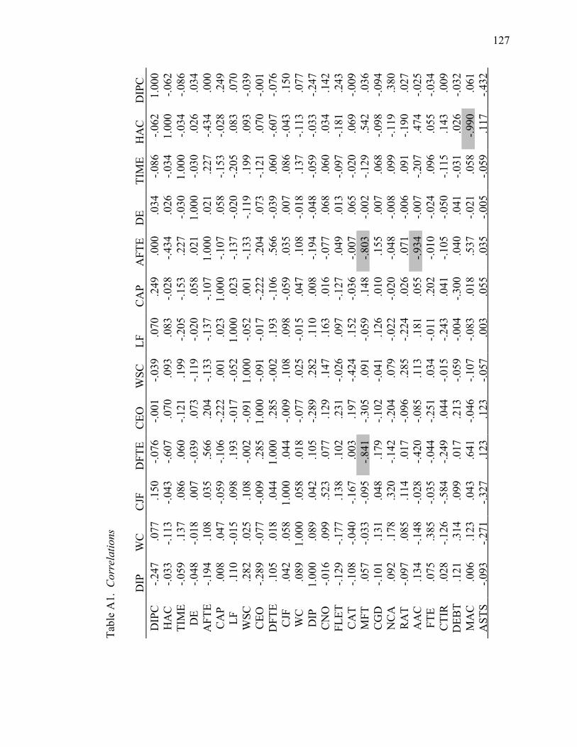
127
DIP
C
1.0
00
-.062
-.086
.034
.000
.249
.070
-.039
-.001
-.076
.150
.077
-.247
.142
.243
-.009
.036
-.094
.380
.027
-.025
-.034
.009
-.032
.061
-.432
HA
C
-.062
1.0
00
-.034
.026
-.434
-.028
.083
.093
.070
-.607
-.043
-.113
-.033
.034
-.181
.069
.542
-.098
-.119
-.190
.474
.055
.143
.026
-.990
.117
TIM
E
-.086
-.034
1.0
00
-.030
.227
-.153
-.205
.199
-.121
.060
.086
.137
-.059
.060
-.097
-.020
-.129
.068
.099
.091
-.207
.096
-.115
-.031
.058
-.059
DE
.034
.026
-.030
1.0
00
.021
.058
-.020
-.119
.073
-.039
.007
-.018
-.048
.068
.013
.065
-.002
.007
-.008
-.006
-.007
-.024
-.050
.041
-.021
-.005
AF
TE
.000
-.434
.227
.021
1.0
00
-.107
-.137
-.133
.204
.566
.035
.108
-.194
-.077
.049
-.007
-.803
.155
-.048
.071
-.934
-.010
-.105
.040
.537
.035
CA
P
X .2
49
-.028
-.153
.058
-.107
1.0
00
.023
.001
-.222
-.106
-.059
.047
.008
.016
-.127
-.036
.148
.010
-.020
.026
.055
.202
.041
-.300
.018
.055
LF
.070
.083
-.205
-.020
-.137
.023
1.0
00
-.052
-.017
.193
.098
-.015
.110
.163
.097
.152
-.059
.126
-.022
-.224
.181
-.011
-.243
-.004
-.083
.003
WS
C
R -.039
.093
.199
-.119
-.133
.001
-.052
1.0
00
-.091
-.002
.108
.025
.282
.147
-.026
-.424
.091
-.041
.079
.285
.113
.034
-.015
-.059
-.107
-.057
CE
O
-.001
.070
-.121
.073
.204
-.222
-.017
-.091
1.0
00
.285
-.009
-.077
-.289
.129
.231
.197
-.305
-.102
-.204
-.096
-.085
-.251
.044
.213
-.046
.123
DF
TE
-.076
-.607
.060
-.039
.566
-.106
.193
-.002
.285
1.0
00
.044
.018
.105
.077
.102
.003
-.841
.179
-.142
.017
-.420
-.044
-.249
.017
.641
.123
CJF
.150
-.043
.086
.007
.035
-.059
.098
.108
-.009
.044
1.0
00
.058
.042
.523
.138
-.167
-.095
.048
.320
.114
-.028
-.035
-.584
.099
.043
-.327
Tab
le A
1. C
orr
elati
ons
Des
crip
tiv
e S
tati
stic
s W
C
.077
-.113
.137
-.018
.108
.047
-.015
.025
-.077
.018
.058
1.0
00
.089
.099
-.177
-.040
-.033
.131
.178
.085
-.148
.385
-.126
.314
.123
-.271
DIP
-.247
-.033
-.059
-.048
-.194
.008
.110
.282
-.289
.105
.042
.089
1.0
00
-.016
-.129
-.108
.057
-.101
.092
-.097
.134
.075
.028
.121
.006
-.093
DIP
C
HA
C
TIM
E
DE
AF
TE
CA
P
X
LF
WS
C
R
CE
O
DF
TE
CJF
WC
DIP
CN
O
C
FL
ET
CA
T
M
MF
T
E
CG
D
P
NC
A
RA
T
M
AA
C
FT
E
CT
IR
DE
BT
MA
C
AS
TS

128
CN
O
C .142
.034
.060
.068
-.077
.016
.163
.147
.129
.077
.523
.099
-.016
1.0
00
.186
-.021
.090
-.207
.228
.021
.028
-.031
-.315
.124
-.023
-.260
FL
ET
.243
-.181
-.097
.013
.049
-.127
.097
-.026
.231
.102
.138
-.177
-.129
.186
1.0
00
.144
-.188
-.164
.216
-.174
-.035
-.858
.010
.126
.184
-.248
CA
T
M -.009
.069
-.020
.065
-.007
-.036
.152
-.424
.197
.003
-.167
-.040
-.108
-.021
.144
1.0
00
.031
-.204
-.103
-.856
.033
-.144
.207
.009
-.065
.100
MF
T
E .
036
.542
-.129
-.002
-.803
.148
-.059
.091
-.305
-.841
-.095
-.033
.057
.090
-.188
.031
1.0
00
-.235
.102
-.019
.646
.160
.227
-.052
-.610
-.081
CG
D
P -.
094
-.098
.068
.007
.155
.010
.126
-.041
-.102
.179
.048
.131
-.101
-.207
-.164
-.204
-.235
1.0
00
-.225
.233
-.087
.254
-.752
-.230
.120
.247
NC
A
.380
-.119
.099
-.008
-.048
-.020
-.022
.079
-.204
-.142
.320
.178
.092
.228
.216
-.103
.102
-.225
1.0
00
.074
-.037
.012
.044
.177
.111
-.950
RA
T
M .0
27
-.190
.091
-.006
.071
.026
-.224
.285
-.096
.017
.114
.085
-.097
.021
-.174
-.856
-.019
.233
.074
1.0
00
-.054
.175
-.287
-.016
.179
-.073
AA
C
-.025
.474
-.207
-.007
-.934
.055
.181
.113
-.085
-.420
-.028
-.148
.134
.028
-.035
.033
.646
-.087
-.037
-.054
1.0
00
-.027
.025
-.043
-.577
.047
FT
E
-.034
.055
.096
-.024
-.010
.202
-.011
.034
-.251
-.044
-.035
.385
.075
-.031
-.858
-.144
.160
.254
.012
.175
-.027
1.0
00
-.114
-.179
-.055
.011
Tab
le A
1. C
orr
elati
ons
(con
t.)
CT
IR
.009
.143
-.115
-.050
-.105
.041
-.243
-.015
.044
-.249
-.584
-.126
.028
-.315
.010
.207
.227
-.752
.044
-.287
.025
-.114
1.0
00
.089
-.151
-.049
DE
BT
-.032
.026
-.031
.041
.040
-.300
-.004
-.059
.213
.017
.099
.314
.121
.124
.126
.009
-.052
-.230
.177
-.016
-.043
-.179
.089
1.0
00
-.020
-.440
MA
C
.061
-.990
.058
-.021
.537
.018
-.083
-.107
-.046
.641
.043
.123
.006
-.023
.184
-.065
-.610
.120
.111
.179
-.577
-.055
-.151
-.020
1.0
00
-.111
AS
TS
-.432
.117
-.059
-.005
.035
.055
.003
-.057
.123
.123
-.327
-.271
-.093
-.260
-.248
.100
-.081
.247
-.950
-.073
.047
.011
-.049
-.440
-.111
1.0
00
DIP
C
HA
C
TIM
E
DE
AF
TE
CA
P
X
LF
WS
C
R
CE
O
DF
TE
CJF
WC
DIP
CN
O
C
FL
ET
CA
T
M
MF
T
E
CG
D
P
NC
A
RA
T
M
AA
C
FT
E
CT
IR
DE
BT
MA
C
AS
TS

129
APPENDIX B
Air Carrier Data
B1 Data Removed due to Listwise Deletion
B2 Air Carrier Specific Data Collection Issues

130
Table B1. Data Removed due to Listwise Deletion.
Training
Data Set
Air Carriers
Removed due to
Listwise Deletion
Number of
Air Carriers
used for
MLM
Valid
Cases
Excluded
Cases
Total
Cases
L1 ATL, TWA1 18 196 64 260
L2 ATL, TWA1 18 212 48 260
L3 ATL, TWA1 18 197 63 260
L4 TWA1 19 213 47 260
L5 ATL 19 214 46 260

Table C2. Air Carrier Specific Data Collection Issues.
Air Carrier Year Quarter Data Issue
Allegiant Air 2002 -
2003 1-4 All
Due to air carrier size, Allegiant was considered a
small carrier for part of the data collection period.
Biannual measurements were divided in half to
calculate quarterly income statement values. Q2 and
Q4 Balance sheet values were used for the quarter
prior's values due the biannual measurement period.
Aloha Airlines 2008 1 Aircraft Operated Value not reported to DOT. The previous quarters
value was used.
Aloha Airlines CEO The CEO was replaced prior to the quarter filing
bankruptcy.
ATA Airlines 2004 4 Aircraft Operated No values reported to DOT for 2004. 2003 count was
used for pre-bankruptcy value.
ATA Airlines 2007 1-4 Aircraft Operated No values reported to DOT for 2007. 2006 count was
used.
Atlas Air/Polar Air
Cargo 2004 1 Aircraft Operated
2003 Q4 value was used as it was more accurate than
the 2004 Q1 value which included two months of
changes in bankruptcy.
America West Airlines 1991 2 Aircraft Operated Value not reported to DOT and unable to find. Value
remains missing.
Braniff International 1982 2 Employees Value not reported to DOT; 1981 value used.
Braniff International Financial
1983 (Q3, Q4) 1984 (Q1) not reported to DOT. Post-
bankruptcy data began with data 4 quarters after
emerging.
Continental Airlines 1 1983 3 Aircraft Operated Value not reported to DOT and unable to find. Value
remains missing.
Continental Airlines 1 1983 3 Employees Value not reported to DOT; 1982 value used.
131

Hawaiian Airlines 1 CEO The CEO was replaced prior to the quarter filing
bankruptcy.
Markair 1992 2 Aircraft Operated Value not reported to DOT and unable to find. Value
remains missing.
Mesa Air 2013 1 Aircraft Operated No values reported to DOT. 2012 Q4 count was used.
Sun Country 1 2002 3 Employees No values reported to DOT. Value interpolated on
quarters before and after.
Sun Country Airlines 2 CEO The CEO was replaced prior to the quarter filing
bankruptcy.
Sun Country Airlines 2 2013 1 Aircraft Operated No values reported to DOT. 2012 Q4 count was used.
Trans World Airlines 1 1993-1995 1-4 Aircraft Operated Value not reported to DOT and unable to find. Value
remains missing.
Trans World Airlines 2 CEO The CEO was replaced prior to the quarter filing
bankruptcy.
United Airlines 2008 4 Retained Earnings
DOT Form 41 data says 11,001,432 and is incorrect
based on Balance Sheet analysis. 2008 annual report
says 5,199,000. Replaced with 5,199,000.
US Airways 1 CEO The CEO was replaced prior to the quarter filing
bankruptcy.
US Airways 2 CEO The CEO was replaced prior to the quarter filing
bankruptcy.
132

133
APPENDIX C
Air Carrier W-Score, P-Score and Restructuring Strategy
C1 Allegiant Air
C2 Aloha Airlines
C3 ATA Airlines
C4 Atlas Air/Polar Air Cargo
C5 America West Airlines
C6 Braniff International
C7 Comair
C8 Continental Airlines 1st Bankruptcy
C9 Continental Airlines 2nd Bankruptcy
C10 Delta Airlines
C11 Frontier Airlines
C12 Hawaiian Airlines 1st Bankruptcy
C13 Hawaiian Airlines 2nd Bankruptcy
C14 Kitty Hawk
C15 Markair
C16 Mesa Air
C17 Mesaba Airlines
C18 Northwest Airlines
C19 Sun Country 1st Bankruptcy
C20 Sun Country Airlines 2nd Bankruptcy
C21 Trans World Airlines 1st Bankruptcy
C22 Trans World Airlines 2nd Bankruptcy

134
C23 United Airlines
C24 US Airways 1st Bankruptcy
C25 US Airways 2nd Bankruptcy

135
Figure C1. Allegiant Air W-Score and P-Score.
Table C1. Allegiant Air Restructuring Strategy.
Variable
Bankrupt
Period
Final
Restructuring
Period
Restructuring
Change
ASTS 4,620 64,005 +1285%
CATM 1.19 0.77 -35%
DEBT 14,677 56,227 +283%
DIP 0 0 No DIP
AAC 1,113,354 3,155,953 +183%
TIME 0 12 N/A
WSCR 7.46 -4.15
P-Score 99.94% 1.55% -98.40 pts.
-15
-5
5
15
0 1 2 3 4 5 6 7 8 9 10 11 12WS
CR
Time
ALLG
0%
20%
40%
60%
80%
100%
0 1 2 3 4 5 6 7 8 9 10 11 12
P-S
core
Pro
bab
ilit
y o
f B
an
kru
ptc
y
Time
ALLG

136
Figure C2. Aloha Airlines W-Score and P-Score.
Table C2. Aloha Airlines Restructuring Strategy.
Variable
Bankrupt
Period
Final
Restructuring
Period
Restructuring
Change
ASTS 152,833 216,951 +42%
CATM 1.02 1.32 +30%
DEBT 305,302 304,152 -0%
DIP 0 1 Yes DIP
AAC 3,594,859 3,491,081 -3%
TIME 0 9 N/A
WSCR 0.70 0.73
P-Score 66.88% 67.53% 0.66 pts.
-15
-10
-5
0
5
10
15
20
0 1 2 3 4 5 6 7 8 9 10 11 12WS
CR
Time
ALOH
0%
20%
40%
60%
80%
100%
0 1 2 3 4 5 6 7 8 9 10 11 12
P-S
core
Pro
bab
ilit
y o
f B
an
kru
ptc
y
Time
ALOH

137
Figure C3. ATA Airlines W-Score and P-Score.
Table C3. ATA Airlines Restructuring Strategy.
Variable
Bankrupt
Period
Final
Restructuring
Period
Restructuring
Change
ASTS 318,375 404,984 +27%
CATM 1.31 0.68 -48%
DEBT 580,549 377,746 -35%
DIP 0 1 Yes DIP
AAC 9,164,796 47,035,114 +413%
TIME 0 6 N/A
WSCR -2.76 -2.64
P-Score 5.93% 6.67% 0.73 pts.
-15
-10
-5
0
5
10
15
20
0 1 2 3 4 5 6 7 8 9 10 11 12WS
CR
Time
ATA
0%
20%
40%
60%
80%
100%
0 1 2 3 4 5 6 7 8 9 10 11 12
P-S
core
Pro
bab
ilit
y o
f B
an
kru
ptc
y
Time
ATA

138
Figure C4. Atlas Air/Polar Air Cargo W-Score and P-Score.
Table C4. Atlas Air/Polar Air Cargo Restructuring Strategy.
Variable
Bankrupt
Period
Final
Restructuring
Period
Restructuring
Change
ASTS 1,436,383 887,183 -38%
CATM 0.15 0.14 -3%
DEBT 1,461,905 570,508 -61%
DIP 0 1 Yes DIP
AAC 31,190,775 72,633,430 +133%
TIME 0 12 N/A
WSCR -0.04 -5.26
P-Score 48.97% 0.52% -48.45 pts.
-15
-10
-5
0
5
10
15
20
0 1 2 3 4 5 6 7 8 9 10 11 12
WS
CR
Time
ATL
0%
20%
40%
60%
80%
100%
0 1 2 3 4 5 6 7 8 9 10 11 12
P-S
core
Pro
bab
ilit
y o
f B
an
kru
ptc
y
Time
ATL

139
Figure C5. America West Airlines W-Score and P-Score.
Table C5. America West Airlines Restructuring Strategy.
Variable
Bankrupt
Period
Final
Restructuring
Period
Restructuring
Change
ASTS 1,230,116 1,583,725 +29%
CATM 0.58 0.59 +1%
DEBT 1,250,532 937,347 -25%
DIP 0 1 Yes DIP
AAC missing 7,189,374 N/A
TIME 0 12 N/A
WSCR -1.35 -4.12
P-Score 20.56% 1.60% -18.96 pts.
-15
-10
-5
0
5
10
15
20
0 1 2 3 4 5 6 7 8 9 10 11 12
WS
CR
Time
AWA
0%
20%
40%
60%
80%
100%
0 1 2 3 4 5 6 7 8 9 10 11 12
P-S
core
Pro
bab
ilit
y o
f B
an
kru
ptc
y
Time
AWA

140
Figure C6. Braniff International W-Score and P-Score.
Table C6. Braniff International Restructuring Strategy.
Variable
Bankrupt
Period
Final
Restructuring
Period
Restructuring
Change
ASTS 877,546 93,678 -89%
CATM 0.29 0.22 -25%
DEBT 910,637 56,303 -94%
DIP 0 0 No DIP
AAC 7,303,934 12,786,541 +75%
TIME 0 12 N/A
WSCR -0.40 -2.21
P-Score 40.08% 9.85% -30.23 pts.
-15
-10
-5
0
5
10
15
20
0 1 2 3 4 5 6 7 8 9 10 11 12
WS
CR
Time
BRAN
0%
20%
40%
60%
80%
100%
0 1 2 3 4 5 6 7 8 9 10 11 12
P-S
core
Pro
bab
ilit
y o
f B
an
kru
ptc
y
Time
BRAN

141
Figure C7. Comair W-Score and P-Score.
Table C7. Comair Restructuring Strategy.
Variable
Bankrupt
Period
Final
Restructuring
Period
Restructuring
Change
ASTS 2,391,313 945,320 -60%
CATM 1.13 0.78 -30%
DEBT 1,596,267 763,835 -52%
DIP 0 1 Yes DIP
AAC 1,812,075 1,200,116 -34%
TIME 0 12 N/A
WSCR -1.68 -0.61
P-Score 15.68% 35.26% 19.58 pts.
-15
-10
-5
0
5
10
15
20
0 1 2 3 4 5 6 7 8 9 10 11 12
WS
CR
Time
COM
0%
20%
40%
60%
80%
100%
0 1 2 3 4 5 6 7 8 9 10 11 12
P-S
core
Pro
bab
ilit
y o
f B
an
kru
ptc
y
Time
COM

142
Figure C8. Continental Airlines 1st Bankruptcy W-Score and P-Score.
Table C8. Continental Airlines 1st Bankruptcy Restructuring Strategy.
Variable
Bankrupt
Period
Final
Restructuring
Period
Restructuring
Change
ASTS 1,110,287 4,016,479 +262%
CATM 0.31 0.26 -14%
DEBT 1,158,120 3,903,210 +237%
DIP 0 0 No DIP
AAC missing 13,881,224 N/A
TIME 0 12 N/A
WSCR -0.92 -1.69
P-Score 28.44% 15.55% -12.89 pts.
-15
-10
-5
0
5
10
15
20
0 1 2 3 4 5 6 7 8 9 10 11 12
WS
CR
Time
CON1
0%
20%
40%
60%
80%
100%
0 1 2 3 4 5 6 7 8 9 10 11 12
P-S
core
Pro
bab
ilit
y o
f B
an
kru
ptc
y
Time
CON1

143
Figure C9. Continental Airlines 2nd Bankruptcy W-Score and P-Score.
Table C9. Continental Airlines 2nd Bankruptcy Restructuring Strategy.
Variable
Bankrupt
Period
Final
Restructuring
Period
Restructuring
Change
ASTS 3,091,744 4,084,843 +32%
CATM 0.66 0.76 +14%
DEBT 4,816,897 3,694,403 -23%
DIP 0 1 Yes DIP
AAC 7,026,434 5,298,656 -25%
TIME 0 12 N/A
WSCR 0.53 -2.48
P-Score 62.85% 7.76% -55.10 pts.
-15
-10
-5
0
5
10
15
20
0 1 2 3 4 5 6 7 8 9 10 11 12
WS
CR
Time
CON2
0%
20%
40%
60%
80%
100%
0 1 2 3 4 5 6 7 8 9 10 11 12
P-S
core
Pro
bab
ilit
y o
f B
an
kru
ptc
y
Time
CON2

144
Figure C10. Delta Airlines W-Score and P-Score.
Table C10. Delta Airlines Restructuring Strategy.
Variable
Bankrupt
Period
Final
Restructuring
Period
Restructuring
Change
ASTS 19,587,128 44,018,556 +125%
CATM 0.82 1.00 +21%
DEBT 24,075,103 44,173,320 +83%
DIP 0 1 Yes DIP
AAC 10,797,507 9,128,322 -15%
TIME 0 12 N/A
WSCR 0.41 0.54
P-Score 60.08% 63.15% 3.08 pts.
-15
-10
-5
0
5
10
15
20
0 1 2 3 4 5 6 7 8 9 10 11 12
WS
CR
Time
DELT
0%
20%
40%
60%
80%
100%
0 1 2 3 4 5 6 7 8 9 10 11 12
P-S
core
Pro
bab
ilit
y o
f B
an
kru
ptc
y
Time
DELT

145
Figure C11. Frontier Airlines W-Score and P-Score.
Table C11. Frontier Airlines Restructuring Strategy.
Variable
Bankrupt
Period
Final
Restructuring
Period
Restructuring
Change
ASTS 1,088,225 850,555 -22%
CATM 1.00 1.00 -0%
DEBT 982,035 734,089 -25%
DIP 0 1 Yes DIP
AAC 7,933,165 6,267,818 -21%
TIME 0 12 N/A
WSCR -2.37 -2.76
P-Score 8.59% 5.93% -2.65 pts.
-15
-10
-5
0
5
10
15
20
0 1 2 3 4 5 6 7 8 9 10 11 12
WS
CR
Time
FRON
0%
20%
40%
60%
80%
100%
0 1 2 3 4 5 6 7 8 9 10 11 12
P-S
core
Pro
bab
ilit
y o
f B
an
kru
ptc
y
Time
FRON

146
Figure C12. Hawaiian Airlines 1st Bankruptcy W-Score and P-Score.
Table C12. Hawaiian Airlines 1st Bankruptcy Restructuring Strategy.
Variable
Bankrupt
Period
Final
Restructuring
Period
Restructuring
Change
ASTS 119,475 208,502 +75%
CATM 0.66 0.52 -21%
DEBT 306,522 124,863 -59%
DIP 0 0 No DIP
AAC 6,321,696 8,892,015 +41%
TIME 0 12 N/A
WSCR 4.81 -4.87
P-Score 99.19% 0.76% -98.43 pts.
-15
-10
-5
0
5
10
15
20
0 1 2 3 4 5 6 7 8 9 10 11 12
WS
CR
Time
HAW1
0%
20%
40%
60%
80%
100%
0 1 2 3 4 5 6 7 8 9 10 11 12
P-S
core
Pro
bab
ilit
y o
f B
an
kru
ptc
y
Time
HAW1

147
Figure C13. Hawaiian Airlines 2nd Bankruptcy W-Score and P-Score.
Table C13. Hawaiian Airlines 2nd Bankruptcy Restructuring Strategy.
Variable
Bankrupt
Period
Final
Restructuring
Period
Restructuring
Change
ASTS 240,105 848,712 +253%
CATM 0.58 0.72 +23%
DEBT 398,860 810,069 +103%
DIP 0 0 No DIP
AAC 11,223,578 11,467,651 +2%
TIME 0 12 N/A
WSCR 0.01 -3.09
P-Score 50.13% 4.34% -45.80 pts.
-15
-10
-5
0
5
10
15
20
0 1 2 3 4 5 6 7 8 9 10 11 12
WS
CR
Time
HAW2
0%
20%
40%
60%
80%
100%
0 1 2 3 4 5 6 7 8 9 10 11 12
P-S
core
Pro
bab
ilit
y o
f B
an
kru
ptc
y
Time
HAW2

148
Figure C14. Kitty Hawk W-Score and P-Score.
Table C14. Kitty Hawk Restructuring Strategy.
Variable
Bankrupt
Period
Final
Restructuring
Period
Restructuring
Change
ASTS 181,878 7,582 -96%
CATM 0.45 0.03 -94%
DEBT 98,428 4,309 -96%
DIP 0 0 No DIP
AAC 2,724,087 1,881,754 -31%
TIME 0 12 N/A
WSCR -7.38 -6.60
P-Score 0.06% 0.14% 0.07 pts.
-15
-10
-5
0
5
10
15
20
0 1 2 3 4 5 6 7 8 9 10 11 12
WS
CR
Time
KITT
0%
20%
40%
60%
80%
100%
0 1 2 3 4 5 6 7 8 9 10 11 12
P-S
core
Pro
bab
ilit
y o
f B
an
kru
ptc
y
Time
KITT

149
Figure C15. Markair W-Score and P-Score.
Table C15. Markair Restructuring Strategy.
Variable
Bankrupt
Period
Final
Restructuring
Period
Restructuring
Change
ASTS 205,980 150,600 -27%
CATM 0.59 0.67 +13%
DEBT 201,203 222,219 +10%
DIP 0 0 No DIP
AAC missing 7,822,636 N/A
TIME 0 5 N/A
WSCR -0.96 0.41
P-Score 27.78% 60.14% 32.36 pts.
-15
-10
-5
0
5
10
15
20
0 1 2 3 4 5 6 7 8 9 10 11 12
WS
CR
Time
MARK
0%
20%
40%
60%
80%
100%
0 1 2 3 4 5 6 7 8 9 10 11 12
P-S
core
Pro
bab
ilit
y o
f B
an
kru
ptc
y
Time
MARK

150
Figure C16. Mesa Air W-Score and P-Score.
Table C16. Mesa Air Restructuring Strategy.
Variable
Bankrupt
Period
Final
Restructuring
Period
Restructuring
Change
ASTS 1,233,140 748,187 -39%
CATM 1.04 0.65 -38%
DEBT 1,011,178 739,909 -27%
DIP 0 0 No DIP
AAC 2,311,618 1,731,746 -25%
TIME 0 9 N/A
WSCR -1.94 -1.28
P-Score 12.62% 21.76% 9.15 pts.
-15
-10
-5
0
5
10
15
20
0 1 2 3 4 5 6 7 8 9 10 11 12
WS
CR
Time
MESA
0%
20%
40%
60%
80%
100%
0 1 2 3 4 5 6 7 8 9 10 11 12
P-S
core
Pro
bab
ilit
y o
f B
an
kru
ptc
y
Time
MESA

151
Figure C17. Mesaba Airlines W-Score and P-Score.
Table C17. Mesaba Airlines Restructuring Strategy.
Variable
Bankrupt
Period
Final
Restructuring
Period
Restructuring
Change
ASTS 151,955 121,341 -20%
CATM 1.09 0.55 -49%
DEBT 103,426 66,792 -35%
DIP 0 1 Yes DIP
AAC 920,055 1,782,318 +94%
TIME 0 12 N/A
WSCR -5.93 -9.56
P-Score 0.26% 0.01% -0.26 pts.
-15
-10
-5
0
5
10
15
20
0 1 2 3 4 5 6 7 8 9 10 11 12
WS
CR
Time
MESB
0%
20%
40%
60%
80%
100%
0 1 2 3 4 5 6 7 8 9 10 11 12
P-S
core
Pro
bab
ilit
y o
f B
an
kru
ptc
y
Time
MESB

152
Figure C18. Northwest Airlines W-Score and P-Score.
Table C18. Northwest Airlines Restructuring Strategy.
Variable
Bankrupt
Period
Final
Restructuring
Period
Restructuring
Change
ASTS 18,706,101 19,289,102 +3%
CATM 0.89 0.98 +10%
DEBT 17,412,776 17,187,256 -1%
DIP 0 1 Yes DIP
AAC 10,390,157 9,069,580 -13%
TIME 0 11 N/A
WSCR -1.52 -0.98
P-Score 17.92% 27.29% 9.37 pts.
-15
-10
-5
0
5
10
15
20
0 1 2 3 4 5 6 7 8 9 10 11 12
WS
CR
Time
NWA
0%
20%
40%
60%
80%
100%
0 1 2 3 4 5 6 7 8 9 10 11 12
P-S
core
Pro
bab
ilit
y o
f B
an
kru
ptc
y
Time
NWA

153
Figure C19. Sun Country 1st Bankruptcy W-Score and P-Score.
Table C19. Sun Country 1st Bankruptcy Restructuring Strategy.
Variable
Bankrupt
Period
Final
Restructuring
Period
Restructuring
Change
ASTS 16,526 62,720 +280%
CATM 2.09 0.53 -74%
DEBT 169,326 54,387 -68%
DIP 0 1 Yes DIP
AAC 6,042,941 9,497,791 +57%
TIME 0 12 N/A
WSCR 19.46 -5.05
P-Score 100.00% 0.64% -99.36 pts.
-15
-10
-5
0
5
10
15
20
0 1 2 3 4 5 6 7 8 9 10 11 12
WS
CR
Time
SUN1
0%
20%
40%
60%
80%
100%
0 1 2 3 4 5 6 7 8 9 10 11 12
P-S
core
Pro
bab
ilit
y o
f B
an
kru
ptc
y
Time
SUN1
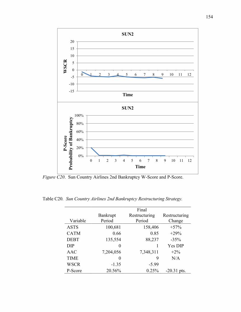
154
Figure C20. Sun Country Airlines 2nd Bankruptcy W-Score and P-Score.
Table C20. Sun Country Airlines 2nd Bankruptcy Restructuring Strategy.
Variable
Bankrupt
Period
Final
Restructuring
Period
Restructuring
Change
ASTS 100,681 158,406 +57%
CATM 0.66 0.85 +29%
DEBT 135,554 88,237 -35%
DIP 0 1 Yes DIP
AAC 7,204,056 7,348,311 +2%
TIME 0 9 N/A
WSCR -1.35 -5.99
P-Score 20.56% 0.25% -20.31 pts.
-15
-10
-5
0
5
10
15
20
0 1 2 3 4 5 6 7 8 9 10 11 12
WS
CR
Time
SUN2
0%
20%
40%
60%
80%
100%
0 1 2 3 4 5 6 7 8 9 10 11 12
P-S
core
Pro
bab
ilit
y o
f B
an
kru
ptc
y
Time
SUN2

155
Figure C21. Trans World Airlines 1st Bankruptcy W-Score and P-Score.
Table C21. Trans World Airlines 1st Bankruptcy Restructuring Strategy.
Variable
Bankrupt
Period
Final
Restructuring
Period
Restructuring
Change
ASTS 2,749,093 2,554,535 -7%
CATM 0.67 0.61 -8%
DEBT 3,633,754 3,089,638 -15%
DIP 0 1 Yes DIP
AAC 39,315,318 missing N/A
TIME 0 7 N/A
WSCR -0.65 -0.92
P-Score 34.30% 28.55% -5.75 pts.
-15
-10
-5
0
5
10
15
20
0 1 2 3 4 5 6 7 8 9 10 11 12
WS
CR
Time
TWA1
0%
20%
40%
60%
80%
100%
0 1 2 3 4 5 6 7 8 9 10 11 12
P-S
core
Pro
bab
ilit
y o
f B
an
kru
ptc
y
Time
TWA1

156
Figure C22. Trans World Airlines 2nd Bankruptcy W-Score and P-Score.
Table C22. Trans World Airlines 2nd Bankruptcy Restructuring Strategy.
Variable
Bankrupt
Period
Final
Restructuring
Period
Restructuring
Change
ASTS 2,554,535 2,928,670 +15%
CATM 0.61 0.68 +12%
DEBT 3,089,638 2,707,383 -12%
DIP 0 0 No DIP
AAC 6,551,698 5,883,974 -10%
TIME 0 12 N/A
WSCR -0.92 -1.79
P-Score 28.55% 14.26% -14.29 pts.
-15
-10
-5
0
5
10
15
20
0 1 2 3 4 5 6 7 8 9 10 11 12
WS
CR
Time
TWA2
0%
20%
40%
60%
80%
100%
0 1 2 3 4 5 6 7 8 9 10 11 12
P-S
core
Pro
bab
ilit
y o
f B
an
kru
ptc
y
Time
TWA2

157
Figure C23. United Airlines W-Score and P-Score.
Table C23. United Airlines Restructuring Strategy.
Variable
Bankrupt
Period
Final
Restructuring
Period
Restructuring
Change
ASTS 24,856,178 19,461,223 -22%
CATM 0.75 1.03 +37%
DEBT 25,697,044 21,927,048 -15%
DIP 0 1 Yes DIP
AAC 10,688,489 12,280,671 +15%
TIME 0 12 N/A
WSCR 0.15 -0.40
P-Score 53.71% 40.03% -13.67 pts.
-15
-10
-5
0
5
10
15
20
0 1 2 3 4 5 6 7 8 9 10 11 12
WS
CR
Time
UNIT
0%
20%
40%
60%
80%
100%
0 1 2 3 4 5 6 7 8 9 10 11 12
P-S
core
Pro
bab
ilit
y o
f B
an
kru
ptc
y
Time
UNIT

158
Figure C24. US Airways 1st Bankruptcy W-Score and P-Score.
Table C24. US Airways 1st Bankruptcy Restructuring Strategy.
Variable
Bankrupt
Period
Final
Restructuring
Period
Restructuring
Change
ASTS 9,953,888 8,497,647 -15%
CATM 0.87 0.95 +9%
DEBT 11,130,845 8,710,038 -22%
DIP 0 1 Yes DIP
AAC 7,920,714 7,319,512 -8%
TIME 0 7 N/A
WSCR 1.23 -1.26
P-Score 77.42% 22.03% -55.39 pts.
-15
-10
-5
0
5
10
15
20
0 1 2 3 4 5 6 7 8 9 10 11 12
WS
CR
Time
USA1
0%
20%
40%
60%
80%
100%
0 1 2 3 4 5 6 7 8 9 10 11 12
P-S
core
Pro
bab
ilit
y o
f B
an
kru
ptc
y
Time
USA1

159
Figure C25. US Airways 2nd Bankruptcy W-Score and P-Score.
Table C25. US Airways 2nd Bankruptcy Restructuring Strategy.
Variable
Bankrupt
Period
Final
Restructuring
Period
Restructuring
Change
ASTS 8,497,647 7,817,772 -8%
CATM 0.95 1.44 +52%
DEBT 8,710,038 6,809,261 -22%
DIP 0 1 Yes DIP
AAC 7,319,512 7,557,887 +3%
TIME 0 12 N/A
WSCR -1.26 -2.64
P-Score 22.03% 6.65% -15.38 pts.
-15
-10
-5
0
5
10
15
20
0 1 2 3 4 5 6 7 8 9 10 11 12
WS
CR
Time
USA2
0%
20%
40%
60%
80%
100%
0 1 2 3 4 5 6 7 8 9 10 11 12
WS
CR
Time
USA2

160
APPENDIX D
Unconditional Growth Model Tables
D1 Data L1 Unconditional Growth Models
D2 Data L3 Unconditional Growth Models
D3 Data L4 Unconditional Growth Models
D4 Data L5 Unconditional Growth Models

161
Table D1. Data L1 Unconditional Growth Models.
Model B Model C Model D
Intercept -.999 (.510) 2.131*** (.603) 2.224*** (.607)
TIME -.210** (.064) -.697*** (.181) -.989** (.314)
TIME2 .044** (.015) .115 (.065)
TIME3 -.004 (.004)
Variance Components
Level 1
(Within) 5.244*** (1.539) 5.112*** (1.567) 5.002*** (1.516)
Level 1 rho 0.774*** (.068) .765*** (.074) .761*** (.075)
Level 2
(Between) .793 (1.346) 1.313 (1.503) 1.385 (1.482)
Level 2 rho
(ICC) .131 .204 .217
Pseudo
R2 .299 .317 .331
Deviance
AIC 835.912 743.637 744.359
BIC 852.948 763.306 767.306
Standard errors are in parentheses. ***p ≤ 0.001 **p ≤ 0.01 *p ≤ 0.05

162
Table D2. Data L2 Unconditional Growth Models.
Model B Model C Model D
Intercept -1.740*** (.419) -1.142* (.483) 2.0168*** (.597)
TIME -.169*** (.041) -.506*** (.141) -1.234*** (.348)
TIME2 .029* (.011) .182** (.069)
TIME3 -.008* (.004)
Variance Components
Level 1
(Within) 4.963*** (.482) 4.822*** (.468) 5.082*** (.516)
Level 1 rho .012 (.105) .009 (.103) -.069 (.112)
Level 2
(Between) 2.137** (.803) 2.169** (.808) 2.482* (.958)
Level 2 rho
(ICC) .301 .310 .328
Pseudo
R2 .155 .179 .135
Deviance
AIC 1116.185 1112.078 995.479
BIC 1133.609 1132.987 1018.975
Standard errors are in parentheses. ***p ≤ 0.001 **p ≤ 0.01 *p ≤ 0.05

163
Table D3. Data L4 Unconditional Growth Models.
Model B Model C Model D
Intercept -1.022** (.412) -.309 (.508) 2.762*** (.596)
TIME -.227*** (.058) -.660*** (.192) -1.320** (.426)
TIME2 .038* (.016) .179* (.086)
TIME3 -.008 (.005)
Variance Components
Level 1
(Within) 6.873*** (.922) 6.653*** (.870) 6.578*** (.841)
Level 1 rho .257* (.130) .246 (.127) .174 (.151)
Level 2
(Between) .443 (.553) .469 (.533) .643 (.571)
Level 2 rho
(ICC) .061 .066 .089
Pseudo
R2 .204 .229 .238
Deviance
AIC 1090.109 1086.616 1025.118
BIC 1107.255 1107.192 1048.648
Standard errors are in parentheses. ***p ≤ 0.001 **p ≤ 0.01 *p ≤ 0.05

164
Table D4. Data L5 Unconditional Growth Models.
Model B Model C Model D
Intercept -1.373** (.456) -.742 (.538) 2.321*** (.653)
TIME -.230*** (.048) -.586** (.171) -1.190** (.411)
TIME2 .030* (.014) .164 (.082)
TIME3 -.008 (.005)
Variance Components
Level 1
(Within) 5.647*** (.731) 5.637*** (.735) 5.956*** (.802)
Level 1 rho .161 (.183) .197 (.159) .175 (.177)
Level 2
(Between) 2.148* (.893) 2.100* (.891) 2.293* (1.000)
Level 2 rho
(ICC) .276 .271 .278
Pseudo
R2 .275 .276 .235
Deviance
AIC 1103.101 1100.589 1024.286
BIC 1120.378 1121.321 1047.848
Standard errors are in parentheses. ***p ≤ 0.001 **p ≤ 0.01 *p ≤ 0.05

165
APPENDIX E
Taxonomy of L3 Dataset Models Table
E1 Taxonomy of L3 Dataset Models

166
Table E1. Taxonomy of L3 Dataset Models.
Model A Model B Model C Model D
Intercept .316 1.552 ** 2.202 *** 2.610 ***
TIME -.239 *** -.612 ** -1.163 **
TIME*TIME .032 .156
TIME*TIME*TIME -.007
TCATM
TCAPX
TLF
TDE
TDIP
TWC
TCEO
TFLET
TCGDP
TCJF
TCNOC
TCTIR
TLOGDFTE
TLOGHAC
TLOGAAC
TLOGDEBT
TLOGASTS
TLOGNCA
TLOGMAC
TAFTE
TMFTE
TFTE
TRATM
Variance Components
Level 1 (Within) 8.709 *** 7.099 *** 6.922 *** 6.813 ***
Level 1 rho .374 ** .192 .182 .170
Level 2 (Between) 1.948 2.318 * 2.379 * 2.387 *
Level 2 rho (ICC) 0.183 .246 .256 .259
Pseudo R2 0.185 0.205 0.218
Deviance
AIC 981.976 971.313 969.896 970.053
BIC 995.109 987.729 989.595 993.036
***p ≤ 0.001 **p ≤ 0.01 *p ≤ 0.05

167
Table E1. Taxonomy of L3 Dataset Models (cont.).
Model E Model F Model G Model H
Intercept 1.271 ** 1.284 ** 1.176 1.265 *
TIME -.191 ** -.193 ** -.182 * -.190 **
TIME*TIME
TIME*TIME*TIME
TCATM 3.031 *** 3.028 *** 2.961 *** 3.051 ***
TCAPX .605
TLF -2.128
TDE .004
TDIP
TWC
TCEO
TFLET
TCGDP
TCJF
TCNOC
TCTIR
TLOGDFTE
TLOGHAC
TLOGAAC
TLOGDEBT
TLOGASTS
TLOGNCA
TLOGMAC
TAFTE
TMFTE
TFTE
TRATM
Variance Components
Level 1 (Within) 6.997 *** 7.016 *** 6.700 *** 6.925 ***
Level 1 rho .309 * .314 * .253 .299 *
Level 2 (Between) 3.128 * 3.071 * 3.263 * 3.129 *
Level 2 rho (ICC) .309 .304 .328 .311
Pseudo R2 0.197 0.194 0.231 0.205
Deviance
AIC 960.985 962.531 962.860 962.555
BIC 980.685 985.513 985.842 985.538
***p ≤ 0.001 **p ≤ 0.01 *p ≤ 0.05

168
Table E1. Taxonomy of L3 Dataset Models (cont.).
Model I Model J Model K Model L
Intercept .544 .676 .522 1.243 *
TIME -.077 -.099 -.071 -.189 **
TIME*TIME
TIME*TIME*TIME
TCATM 4.284 *** 3.965 *** 4.175 *** 2.961 ***
TCAPX
TLF
TDE
TDIP -3.229 *** -3.109 *** -3.145 ***
TWC -.753
TCEO -.271
TFLET .002
TCGDP
TCJF
TCNOC
TCTIR
TLOGDFTE
TLOGHAC
TLOGAAC
TLOGDEBT
TLOGASTS
TLOGNCA
TLOGMAC
TAFTE
TMFTE
TFTE
TRATM
Variance Components
Level 1 (Within) 7.306 *** 7.105 *** 7.227 *** 7.000 ***
Level 1 rho .452 *** .426 *** .445 *** .307 *
Level 2 (Between) 2.724 2.120 2.828 2.920 *
Level 2 rho (ICC) .272 .230 .281 .294
Pseudo R2 0.161 0.184 0.170 0.196
Deviance
AIC 943.859 943.232 945.739 962.428
BIC 966.842 969.498 972.004 985.411
***p ≤ 0.001 **p ≤ 0.01 *p ≤ 0.05

169
Table E1. Taxonomy of L3 Dataset Models (cont.).
Model M Model N Model O Model P
Intercept .875 .758 .835 1.158 *
TIME -.156 * -.124 -.126 -.130
TIME*TIME
TIME*TIME*TIME
TCATM 4.112 *** 4.223 *** 4.029 *** 5.096 ***
TCAPX
TLF
TDE
TDIP
TWC
TCEO
TFLET
TCGDP .377
TCJF .075
TCNOC -.062
TCTIR .000 .000 *** .000 ** .000 ***
TLOGDFTE -1.675
TLOGHAC -8.171
TLOGAAC 6.801 **
TLOGDEBT
TLOGASTS
TLOGNCA
TLOGMAC
TAFTE
TMFTE
TFTE
TRATM
Variance Components
Level 1 (Within) 6.073 *** 6.492 *** 6.660 *** 6.719 ***
Level 1 rho .230 .285 * .301 * .368 **
Level 2 (Between) 3.031 * 2.502 * 1.863 1.047
Level 2 rho (ICC) .333 .278 .219 .135
Pseudo R2 0.303 0.255 0.235 0.228
Deviance
AIC 952.448 949.627 950.613 938.586
BIC 985.280 972.610 976.878 968.135
***p ≤ 0.001 **p ≤ 0.01 *p ≤ 0.05

170
Table E1. Taxonomy of L3 Dataset Models (cont.).
Model Q Model R Model S Model T
Intercept .833 .950 .884 1.340 *
TIME -.114 -.123 -.124 -.169 *
TIME*TIME
TIME*TIME*TIME
TCATM 4.524 *** 4.619 *** 4.277 *** 3.858 ***
TCAPX
TLF
TDE
TDIP
TWC
TCEO
TFLET
TCGDP
TCJF
TCNOC
TCTIR .000 *** .000 *** .000 ***
TLOGDFTE
TLOGHAC
TLOGAAC 3.505 ** 5.141 3.169 * 4.876 ***
TLOGDEBT 21.754 *** 23.300 *** 24.613 *** 23.113 ***
TLOGASTS -20.663 *** -19.094 *** -20.157 *** -22.816 ***
TLOGNCA
TLOGMAC -2.456
TAFTE
TMFTE .102
TFTE .000 .000
TRATM
Variance Components
Level 1 (Within) 5.946 *** 5.697 *** 5.731 *** 6.532 ***
Level 1 rho .334 * .280 .298 * .402 **
Level 2 (Between) 1.486 1.128 1.349 2.270
Level 2 rho (ICC) .200 .165 .191 .258
Pseudo R2 0.317 0.346 0.342 0.250
Deviance
AIC 926.390 928.827 925.516 935.064
BIC 959.222 971.508 961.631 964.613
***p ≤ 0.001 **p ≤ 0.01 *p ≤ 0.05

171
APPENDIX F
Average Values of Significant Predictors
F1 Average CATM
F2 Average AAC
F3 Average DEBT
F4 Average ASTS

172
Figure F1. Average CATM.
Figure F2. Average AAC.
0
0.1
0.2
0.3
0.4
0.5
0.6
0.7
0.8
0.9
0 1 2 3 4 5 6 7 8 9 10 11 12
Aver
age
CA
TM
TIME
0
50
100
150
200
250
300
0 1 2 3 4 5 6 7 8 9 10 11 12
Aver
age
AA
CF
T
(Mil
lion
s)
TIME

173
Figure F3. Average DEBT.
Figure F4. Average ASTS.
0
1
2
3
4
5
6
0 1 2 3 4 5 6 7 8 9 10 11 12
Aver
age
DE
BT
(Bil
lio
ns)
TIME
0
1
2
3
4
5
6
0 1 2 3 4 5 6 7 8 9 10 11 12
Aver
age
AS
TS
(Bil
lion
s)
TIME

174
APPENDIX G
MLM Residuals
G1 Normal Probability Plot of Residuals
G2 Residuals against Predictors

175
Figure G1. Normal probability plot of residuals.
Figure G2. Residuals against predictors.

176
Figure G2. Residuals against predictors (continued).

177
Figure G2. Residuals against predictors (continued).