Efficient Reasoning for Inconsistent Horn Formulae

Joao Marques-Silva1, Alexey Ignatiev1,4, Carlos Mencıa2, and Rafael Penaloza3

1 University of Lisbon, Portugal ({jpms,aignatiev}@ciencias.ulisboa.pt)2 University of Oviedo, Spain (cmencia@gmail.com)

3 Free University of Bozen-Bolzano, Italy (rafael.penaloza@unibz.it)4 ISDCT SB RAS, Irkutsk, Russia

Abstract. Horn formulae are widely used in different settings that include logicprogramming, answer set programming, description logics, deductive databases,and system verification, among many others. One concrete example is conceptsubsumption in lightweight description logics, which can be reduced to inferencein propositional Horn formulae. Some problems require one to reason with in-consistent Horn formulae. This is the case when providing minimal explanationsof inconsistency. This paper proposes efficient algorithms for a number of deci-sion, function and enumeration problems related with inconsistent Horn formu-lae. Concretely, the paper develops efficient algorithms for finding and enumerat-ing minimal unsatisfiable subsets (MUSes), minimal correction subsets (MCSes),but also for computing the lean kernel. The paper also shows the practical impor-tance of some of the proposed algorithms.

1 IntroductionHorn formulae have been studied since at least the middle of the past century [18,

19]. More recently, Horn formulae have been used in a number of different settings,which include logic programming, answer set programming and deductive databases,but also description logics. In addition, there is a growing interest on Horn formulareasoning in formal methods [12, 13]. In the area of description logics, there is a tightrelationship between description logic reasoning and Horn formulae. This is true forlightweight description logics [2,3,5,23,32,42,44,46], but there exists recent work sug-gesting the wider application of Horn formulae to (non-lightweight) description logicreasoning [9].

It is well-known that the decision problem for Horn formulae is in P [18], withlinear-time algorithms known since the 80s [16, 20, 37]. Nevertheless, other decision,function and enumeration problems are of interest when reasoning about Horn formu-lae, which find immediate application in other settings, that include description logics.Moreover, related problems on Horn formulae have been studied earlier in other con-texts [17, 31]. This paper extends earlier work on developing efficient algorithms forreasoning about Horn formulae [3, 5, 42]. Concretely, the paper investigates the com-plexity of finding and enumerating MUSes, MCSes, but also the complexity of com-puting the lean kernel [24–27]. The paper also studies MUS and MCS membership andrelated problems. In addition, the paper also investigates the practical significance ofsome of these new algorithms.

The paper is organized as follows. Section 2 introduces the notation used through-out the paper. Section 3 revisits the well-known linear time unit resolution (LTUR)algorithm, and proposes two algorithms used extensively in the remainder of the paper.Section 4 develops the main results in the paper. The practical significance of the workis briefly addressed in Section 5, before concluding in Section 6.

2 PreliminariesThis section introduces the notation and definitions used throughout the paper. We

assume that the reader is familiar with the basic notions of propositional logic (see e.g.[11]). CNF formulae are defined over a finite set of propositional variables. A literal is avariable or its complement. A clause is a disjunction of literals, also interpreted as a setof literals. A CNF formulaF is a finite conjunction of clauses, also interpreted as a finiteset of clauses. In some settings, it is convenient to view a CNF formula as a multisetof clauses, where the same clause can appear more than once. The set of variablesassociated with a CNF formula F is denoted by var(F). We often use X , var(F),with n , |X|.m , |F| represents the number of clauses in the formula, and the numberof literal occurrences in F is represented by ||F||. An assignment is a mapping fromX from {0, 1}, and total assigments are assumed throughout. Moreover, the semanticsof propositional logic is assumed. For a formula F , we write F 2⊥ (resp. F �⊥) toexpress that F is satisfiable (resp. unsatisfiable).

In this paper we focus on Horn formulae. Intuitively, Horn formulae are sets of im-plications of the form A1 ∧ A2 ∧ . . . ∧ Akj

→ Ij , where all Ar are positive literalsdefined over the variables in X , and Ij is either a positive literal or⊥. Formally, a Hornformula F is a CNF formula where each clause contains at most one positive literal.Clauses without a positive literal are called goal clauses, and those with a positive lit-eral are called definite. Given a (Horn) clause c ∈ F , P (c) denotes the set of variablesappearing positively in c. For Horn clauses, P (c) always contains at most one element.Likewise, N(c) denotes the set of variables appearing negatively in c. We apply a sim-ilar notation for variables v. In this case, N(v) (resp. P (v)) denotes the set of clauseswhere v occurs as a negative (resp. positive) literal.

We are interested in inconsistent formulae F , i.e. F �⊥, such that some clausesin F can be relaxed (i.e. allowed not to be satisfied) to restore consistency, whereasothers cannot. Thus, we assume that F is partitioned into two subformulae F = B∪R,where R contains the relaxable clauses, and B contains the non-relaxable clauses. Bcan be viewed as background knowledge, which must always be kept. As we will seein this paper, allowing B 6= ∅ can affect the computational complexity and the runtimebehavior of the tasks that we consider.

Given an inconsistent CNF formulaF , we are interested in detecting the clauses thatare responsible for unsatisfiability among those that can be relaxed, as defined next.

Definition 1 (Minimal Unsatisfiable Subset (MUS)). Let F = B ∪ R denote an in-consistent set of clauses (F �⊥).M⊆ R is a Minimal Unsatisfiable Subset (MUS) iffB ∪M�⊥ and ∀M′(M, B ∪M′ 2⊥.

⋃MU(F) denotes the union of all MUSes.

Informally, an MUS provides the minimal information that needs to be added to thebackground knowledge B to obtain an inconsistency; thus, it explains the causes for

2

this inconsistency. Alternatively, one might be interested in correcting the formula, re-moving some clauses to achieve consistency.

Definition 2 (MCS,MSS). Let F = B ∪ R denote an inconsistent set of clauses(F �⊥). C ⊆ R is a Minimal Correction Subset (MCS) iff B ∪ R \ C 2⊥ and ∀C′(C ,B∪R\C′ �⊥. We use

⋃MC(F) to denote the union of all MCSes. S ⊆ R is a Maximal

Satisfiable Subset (MSS) iff B ∪ S 2⊥ and ∀S′)S , B ∪ S ′ �⊥.

It is well known that there is a close connection between MUSes, MCSes, and MSSes.Indeed, it is easy to see that a set C is an MCS iff R \ C is an MSS. Moreover, thereexists a minimal hitting set duality between MUSes and MCSes [43]. In particular thismeans that

⋃MU(F) =

⋃MC(F).

The lean kernel [24–27] represents an (easier to compute) over-approximation of⋃MU(F), containing all clauses that can be included in a resolution refutation of F ,

with F �⊥. The lean kernel of a CNF formula is tightly related with the maximumautarky of the formula, one being the complement of the other [24–27]. Computationof the lean kernel for Horn formulae is analyzed in Section 4.3.

For arbitrary CNF formulae, there exists recent work on extracting MUSes [7, 10],and on extracting MCSes [6,33, 35,36]. The complexity of extracting MUSes for Hornformulae has also been studied in the context of so-called axiom pinpointing for light-weight description logics [5, 41, 42]. In particular, it has been shown that axiom pin-pointing for the EL family of description logics [4, 5] can be reduced to the problem ofcomputing MUSes of a Horn formula with B 6= ∅ (see [2, 3, 44] for details).

We also assume that the reader is familiar with the basic notions of computationalcomplexity; for details, see [22, 39, 40]. Throughout the paper, the following abbrevia-tions are used. For decision problems [39], NPC stands for NP-complete, and PNP (or∆p

2) denotes the class of problems that can be decided with a polynomial number ofcalls (on the problem representation) to an NP oracle. Similarly, PNP[log] denotes theclass of problems that can be decided with a logarithmic number of calls to an NP oracle(where n denotes the size of the problem instance). For enumeration problems [22], OPstands for output polynomial and PD stands for polynomial delay, denoting respectivelyalgorithms that run in time polynomial on the size of the input and already computed so-lutions (i.e. the output), and algorithms that compute each solution in time polynomialsolely on the size of the input. Finally, for function (or search problems), the notationused for characterizing the complexity of decision problems is prefixed with F [39]. Forexample, FPNP denotes the class of function problems solved with a polynomial num-ber of calls to an NP oracle. Similarly, FPNP[log] (respectively FPNP[wit,log]) denotes theclass of function problems solved with a logarithmic number of calls to an NP oracle(respectively to a witness producing NP oracle [14]).

3 Basic LTUR and SaturationIt is well-known that consistency of Horn formulae can be decided in linear time

on the size of the formula [16,20,37]. A simple algorithm that achieves this linear-timebehavior on the number of literals appearing in the formula, is known as linear time unitresolution (LTUR) [37]. Motivated by the different uses in the remainder of the paper,a possible implementation is analyzed next. In addition, we also introduce an extension

3

Function LTUR(F)Input : F : input Horn formulaOutput: falsified clause, if any; α: antecedents

1 (Q, η, γ, α)← Initialize(F)2 while Q 6= ∅ do // Q: queue of variables assigned 13 vj ← ExtractFirstVariable(Q)4 foreach ci ∈ N(vj) do5 η(ci)← η(ci)− 16 if η(ci) = 0 then7 if γ(ci) then return ({ci}, α)8 vr ← PickVariable(P (ci))9 if α(vr) = ∅ then

10 AppendToQueue(Q, vr)11 α(vr)← {ci}12 return (∅, α)

Algorithm 1: The LTUR algorithm

of LTUR that saturates the application of unit propagation rules, without affecting thelinear-time behavior. We then show how the result of this saturation can be used to tracethe causes of all consequences derived by LTUR.

3.1 Linear Time Unit Resolution

LTUR can be viewed as one-sided unit propagation, in the sense that only variablesassigned value 1 are propagated. The algorithm starts with all variables assigned value0, and repeatedly flips variables to 1, one at a time. Let η : F → N0 associate a counterwith each clause, representing the number of negative literals not assigned value 0.Given an assignment, a goal clause c ∈ F is falsified if η(c) = 0. Similarly, a definiteclause c ∈ F is unit and requires the sole positive literal to be assigned value 1 whenη(c) = 0. LTUR maintains the η counters, propagates assignments due to unit definiteclauses and terminates either when a falsified goal clause is identified or when no moredefinite clauses require that their sole positive literal be assigned value 1. The procedurestarts with unit positive clauses cr for which η(cr) = 0. Clearly, a Horn formula withoutunit positive clauses is trivially satisfied. In the following, γ : F → {0, 1} denoteswhether a clause c ∈ F is a goal clause, in which case γ(c) = 1. Finally, α : var(F)→2F is a function that assigns to each variable v a set of clauses α(v) that are deemedresponsible for assigning value 1 to v. If the value of v is not determined to be 1, thenα(v) = ∅. As is standard in CDCL SAT solving [11], α(v) will be referred to as theantecedent (set) of v. The organization of LTUR is summarized in Algorithm 1. Theinitialization step sets the initial values of the η counters, the α values, and the valueof the γ flag. Q is initialized with the variables in the unit positive clauses. For everyv ∈ Q, α(v) contains the unit clause v. For all other variables, the value of α is ∅.Clearly, this initialization runs in time linear on the number of literals. The main loopanalyzes the variables assigned value 1 in order. Notice that a variable v is assignedvalue 1 iff α(v) 6= ∅. For each variable v ∈ Q, the counter η of the clauses where voccurs as a negative literal is decreased. If the η(c) = 0 for some clause c, then eitherthe formula is inconsistent, if c is a goal clause, or the positive literal of c is assigned

4

Function LTURS(F)Input : F : input Horn formulaOutput: U : falsified clauses; α: antecedent sets

1 (Q, η, γ, α,U)← Initialize(F)2 while Q 6= ∅ do // Q: queue of variables assigned 13 vj ← ExtractFirstVariable(Q)4 foreach ci ∈ N(vj) do5 η(ci)← η(ci)− 16 if η(ci) = 0 then7 if γ(ci) then8 U ← U ∪ {ci}9 else

10 vr ← PickVariable(P (ci))11 if α(vr) = ∅ then12 AppendToQueue(Q, vr)13 α(vr)← α(vr) ∪ {ci}14 return (U , α)

Algorithm 2: The LTURs algorithm

value 1 and added toQ. The operation of LTUR is such that |α(v)| ≤ 1 for v ∈ var(F).It is easy to see that LTUR runs in linear time on the number of literals of F [37]: eachvariable v is analyzed only once, since v is added to the queue Q only if α(v) = ∅,and after being added to Q, α(v) 6= ∅ and α(v) will not be set to ∅ again. Thus, v willnot be added to Q more than once. For each variable v, its clauses are analyzed at mostonce, in case v was added to Q. Thus, the number of times literals are analyzed duringthe execution of LTUR is O(||F||).

It is often convenient to run LTUR incrementally. Given F = R∪B, one can add aunit positive clause at a time, and run LTUR while consistency is preserved. If no incon-sistency is identified for any of the unit positive clauses, the total run time isO(||F||). Incontrast, if inconsistency is identified for some unit positive clause, consistency may berecovered by undoing only the last sequence of variables assigned value 1. IncrementalLTUR plays an important role in the algorithms described in Section 4, concretely forMUS and MCS extraction.

3.2 LTUR SaturationWe will often resort to a modified version of LTUR, which we call LTUR satura-

tion (LTURs). LTURs also runs in linear time on the number of literals, but exhibitsproperties that are relevant when analyzing inconsistent Horn formulae. The basic ideais not to terminate the execution of LTUR when a falsified goal clause is identified.Instead, the falsified clause is recorded, and the one-sided unit propagation of LTURcontinues to be executed. The procedure only terminates when Q is empty. Besides U ,in this case the value of α(v) is updated with any clause that can serve to determiningthe assignment of v to value 1.

Algorithm 2 summarizes the main steps of LTURs. When compared with LTUR,the main difference is the set U , initially set to ∅, and to which the falsified clausesare added to. Using the same arguments presented in Section 3.1, it can be shown thatLTURs also runs in time O(||F||).

5

Function TRACECLAUSES(U , α)Input : U : falsified clause(s); α: antecedentsOutput:M: traced clauses from F , given U and α

1 (S,M, φ)← INITIALIZE(U)2 while not EMPTY(S) do3 ci ← POPCLAUSE(S)4 foreach vr ∈ N(ci) do5 foreach ca ∈ α(vr) do6 if φ(ca) = 0 then7 φ(ca)← 18 PUSHCLAUSE(S, ca)9 M←M∪ {ca}10 returnM

Algorithm 3: Tracing antecedents

Table 1: Summary of results

B? 1 MUS MUS Enum 1 MCS MCS Enum Lean Kernel ∈MUS ∈MCS⋃

MU,⋃

MC

B = ∅ linear PD linear PD linear NPC NPC FPNP[wit,log]

B 6= ∅ poly not OP poly not OP linear NPC NPC FPNP[wit,log]

3.3 Tracing AntecedentsAnother important step when analyzing inconsistent Horn formulae is to trace an-

tecedents. Algorithm 3 describes an approach for tracing that is based on knowing atleast one antecedent for each variable assigned 1. Thus, this method can be used afterrunning LTUR or LTURs. In the algorithm, φ is used as a flag to ensure each clauseis traced at most once. The stack S is initialized with the clauses in U . Algorithm 3implements a depth-first traversal of the graph induced by the antecedent sets, startingfrom the clauses in U . Hence, the algorithm runs in O(||F||) time.

4 Efficient Reasoning for Inconsistent Horn FormulaeIn this section we analyze a number of computational problems related with the

analysis of inconsistent Horn formulae. The main results obtained are summarizedin Table 1. Some of the results, depicted with slanted text, are adapted from the lit-erature. We briefly recall these results before presenting our contributions.

An algorithm for enumerating all MUSes of an inconsistent Horn formula with-out background knowledge can be obtained through a straightforward modification ofthe method presented in [42]. In the presence of background knowledge (that is, whenB 6= ∅), it was shown in [5, Theorem 4] that no output polynomial algorithm exists forenumerating all MUSes (unless P = NP). A similar approach was used to prove thatMCSes for formulae with background knowledge cannot be enumerated in output poly-nomial time in [41, Theorem 6.15], unless P = NP. In [42, Theorems 17, 18] is was alsoshown that deciding MUS membership for a clause is NP-complete. A simple algorithmfor finding one MUS requires one inconsistency check for every relaxable clause in theformula [8, 15]. The linear runtime of LTUR [16, 37] guarantees that one MUS can becomputed in quadratic time. This upper bound was further refined to O(|M| · ||F||),

6

whereM is the size of the largest MUS, in [3]. In the following we provide more detailson these results, and prove the remaining claims from Table 1.

4.1 MUS Extraction and EnumerationWe first focus on the problems related to extracting and enumerating MUSes. As

mentioned already, to compute one MUS one can simply perform a linear number of in-consistency tests—one for each clause inR. This yields an overall quadratic behaviour.As we show next, in the absence of background knowledge, one MUS can be extractedin linear time.

Proposition 1 (MUS Extraction, B = ∅). Let F �⊥, with B = ∅. One MUS of F canbe computed in time O(||F||).

Proof. Horn formulae are decided by LTUR, that implements (one-sided) unit propaga-tion and runs inO(||F||). It is well-known that unsatisfiable subsets computed with unitpropagation are MUSes [29, Proposition 1]. Thus, tracing antecedents, starting from thefalsified goal clause c ∈ F returned by LTUR, yields an MUS of F . Algorithm 3 il-lustrates an implementation of clause tracing that runs inO(||F||). Overall, both LTURand clause tracing are run once. Hence, an MUS is extracted in time O(||F||). ut

One important observation is that the polynomial delay enumeration algorithm pre-sented in [42] uses an arbitrary polynomial-time MUS extraction algorithm as a black-box. Thus, the linear time extraction method presented above can be exploited to enu-merate all MUSes more efficiently.

When the formula F contains background knowledge, MUS extraction becomesmore expensive. As shown recently in [3] through an insertion-based algorithm, in thiscase an MUS can be computed in O(|M| · ||F||) time, where M is the size of thelargest MUS. This is achieved by running LTUR incrementally, allowing the run timeof successive consistent runs of LTUR to amortize to ||F||. Unfortunately, backgroundknowledge has a more important effect on the enumeration problem. Indeed, as shownin [5], if B 6= ∅, it is impossible to enumerate all MUSes in output polynomial time,unless P = NP.

4.2 MCS Extraction and EnumerationA simple algorithm for computing one MCS consists in running LTUR first over

all the clauses in B, and then incrementally adding each clause c in R = F \ B tothe execution of LTUR. As soon as LTUR detects an inconsistency, the latest clause cinserted is known to belong to an MCS and is added to a set C; this clause is retracted,and the process continues. When all clauses have been tested, C contains an MCS,and its complement is an MSS. Overall, by running LTUR incrementally, the consistentcalls to LTUR amortize to ||F||. For the inconsistent calls to LTUR, i.e. those producingclauses added to C, one needs to undo the incremental run of LTUR, which in the worst-case runs in ||F||. This process needs to be executed once for each clause in C. Takinginto account that the (amortized) running time of LTUR is O(||F||), an MCS can becomputed in time O(|C| · ||F||), where C is the size of the largest MCS in F .

As it was the case for MUSes, the MCS extraction procedure can be improved to runin linear time in the case where B = ∅. Consider again the execution of LTURs (see Al-

7

Function MCSENUM(F , τ)Global : M: MCS registerInput : F : input Horn formula; τ : clause tags

1 (U , α)← LTURs(F) // Use LTUR saturation to find MCS candidate2 if U = ∅ then return3 (C,V)← PickVariables(U) // V: variables of negative literals in U4 if MCSRegistered(C,M) then return5 RegisterMCS(C,M) // Record computed MCS in MCS register6 foreach v ∈ V do7 W ← DropClauses(F ,¬v) // Drop clauses with literal ¬v

// Next, drop literal v in clauses ofW and tag clauses8 (W, τ)← DropLitsTagCls(W, τ, v)9 MCSENUM(W, τ) // Recursive call of MCS enumeration

Algorithm 4: MCS enumeration with polynomial delay

gorithm 2). Since B = ∅, any clause can be included in an MCS. This observation yieldsthe following result.

Proposition 2. Given F , with F �⊥, the set U computed by LTURs is an MCS of F .

Proof. First, we show that U is a correction set. Observe that U is composed of goalclauses. Goal clauses do not serve to propagate other variables to value 1 and do notserve to prevent variables from being assigned value 1 when running LTURs. Thus,removing these clauses will not elicit further propagation of variables to value 1. Sincethese are the only falsified clauses, if the clauses in U are removed, what remains issatisfiable; hence U is a correction set. To show that U is minimal, observe that if anyclause in U is not removed, then it will remain unsatisfied, again because removingclauses in U does not alter the variables assigned value 1. Thus, U is a correction set forF and it is minimal, and so it is an MCS for F . ut

Corollary 1. LTURs computes an MCS in linear time on the number of literals.

In different settings, enumeration of MUSes and MCSes is paramount [5, 42, 44]. Wecan use the linear time algorithm for MCS extraction to develop a polynomial delayalgorithm for enumerating MCSes of a Horn formula when B = ∅. We know how tocompute one MCS in linear time, by applying LTURs and falsifying goal clauses. Thequestion is then how to iterate the computation of MCSes. The approach we follow is totransform the formula, so that different sets of falsified goal clauses are obtained. Givena goal clause c with a negative literal ` on variable v, the transformation is to removethe clauses with literal ¬v, and remove the literal v from each clause c′ containing thatliteral. The resulting clause cr = c′ \ {v} becomes a goal clause. The newly createdgoal clause is tagged with the variable v. As the formula is transformed, τ(c) indicateswhether c is tagged, taking value ⊥ if not, or being assigned some variable otherwise.As a result, when LTURs is used to find a set of falsified goal clauses, the computedMCSes must also account for the set of tags associated with these falsified goal clauses.

Algorithm 4 summarizes the main steps of the MCS enumeration algorithm withpolynomial delay. At each step, LTURs is used to find a set of falsified goal clauses

8

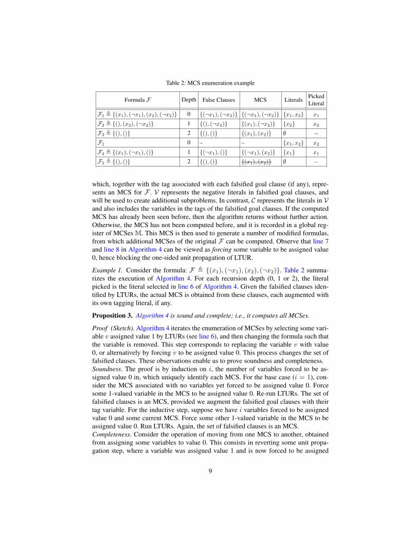
Table 2: MCS enumeration example

Formula F Depth False Clauses MCS Literals PickedLiteral

F1 , {(x1), (¬x1), (x2), (¬x2)} 0 {(¬x1), (¬x2)} {(¬x1), (¬x2)} {x1, x2} x1

F2 , {(), (x2), (¬x2)} 1 {(), (¬x2)} {(x1), (¬x2)} {x2} x2

F3 , {(), ()} 2 {(), ()} {(x1), (x2)} ∅ –

F1 0 – – {x1, x2} x2

F4 , {(x1), (¬x1), ()} 1 {(¬x1), ()} {(¬x1), (x2)} {x1} x1

F5 , {(), ()} 2 {(), ()} {(x1), (x2)} ∅ –

which, together with the tag associated with each falsified goal clause (if any), repre-sents an MCS for F . V represents the negative literals in falsified goal clauses, andwill be used to create additional subproblems. In contrast, C represents the literals in Vand also includes the variables in the tags of the falsified goal clauses. If the computedMCS has already been seen before, then the algorithm returns without further action.Otherwise, the MCS has not been computed before, and it is recorded in a global reg-ister of MCSes M. This MCS is then used to generate a number of modified formulas,from which additional MCSes of the original F can be computed. Observe that line 7and line 8 in Algorithm 4 can be viewed as forcing some variable to be assigned value0, hence blocking the one-sided unit propagation of LTUR.

Example 1. Consider the formula: F , {(x1), (¬x1), (x2), (¬x2)}. Table 2 summa-rizes the execution of Algorithm 4. For each recursion depth (0, 1 or 2), the literalpicked is the literal selected in line 6 of Algorithm 4. Given the falsified clauses iden-tified by LTURs, the actual MCS is obtained from these clauses, each augmented withits own tagging literal, if any.

Proposition 3. Algorithm 4 is sound and complete; i.e., it computes all MCSes.

Proof (Sketch). Algorithm 4 iterates the enumeration of MCSes by selecting some vari-able v assigned value 1 by LTURs (see line 6), and then changing the formula such thatthe variable is removed. This step corresponds to replacing the variable v with value0, or alternatively by forcing v to be assigned value 0. This process changes the set offalsified clauses. These observations enable us to prove soundness and completeness.Soundness. The proof is by induction on i, the number of variables forced to be as-signed value 0 in, which uniquely identify each MCS. For the base case (i = 1), con-sider the MCS associated with no variables yet forced to be assigned value 0. Forcesome 1-valued variable in the MCS to be assigned value 0. Re-run LTURs. The set offalsified clauses is an MCS, provided we augment the falsified goal clauses with theirtag variable. For the inductive step, suppose we have i variables forced to be assignedvalue 0 and some current MCS. Force some other 1-valued variable in the MCS to beassigned value 0. Run LTURs. Again, the set of falsified clauses is an MCS.Completeness. Consider the operation of moving from one MCS to another, obtainedfrom assigning some variables to value 0. This consists in reverting some unit propa-gation step, where a variable was assigned value 1 and is now forced to be assigned

9

value 0. The algorithm reverts unit propagation steps in order, creating a search tree.Each node in this search tree represents one MCS and is expanded into k children. Eachchild node is associated with one of the 1-valued literals in the MCS to be forced to beassigned value 0. Thus, Algorithm 4 will enumerate all subsets of variables assignedvalue 1, which lead to a conflict being identified, and so all MCSes are enumerated. ut

Proposition 4. Algorithm 4 enumerates the MCSes of an inconsistent Horn formula Fwith polynomial delay.

Proof (Sketch). At each iteration, Algorithm 4 runs LTURs in linear time, and trans-forms the current working formula, also a linear time operation, once for each literalin the target set of literals. The algorithm must check whether the MCS has alreadybeen computed, which can be done in time logarithmic on the number of MCSes storedin the MCS registry, e.g. by representing the registry with a balanced search tree. Theadditional work done by Algorithm 4 in between computed MCSes is polynomial onthe formula size. The iterations that do not produce an MCS are bounded by a polyno-mial as follows. An MCS can be repeated from a recursive call, but only after one newMCS is computed. Each new MCS can recursively call Algorithm 4 O(|F|) times, inthe worst-case each call leading to an MCS not being computed. Thus, the overall costof recursive calls to Algorithm 4 leading to an MCS not being computed is polynomial.Therefore, Algorithm 4 computes MCSes of an inconsistent Horn formula with poly-nomial delay. ut

4.3 Finding the Lean KernelThe lean kernel is the set of all clauses that can be used in some resolution refutation

of a propositional formula, and has been shown to be tightly related with the conceptof maximum autarky [24–26]. Autarkies were proposed in the mid 80s [38] with thepurpose of devising an algorithm for satisfiability requiring less than 2n steps. Laterwork revealed the importance of autarkies when analyzing inconsistent formulas [24,25,27,34]. Indeed, the lean kernel represents an over-approximation of

⋃MU [24–27],

that is in general easier to compute for arbitrary CNF formulae. As shown in this section,the same holds true for Horn formulae.

Example 2. Consider the Horn formula:F , {(a), (¬a∨b), (¬b∨x), (¬x∨b), (¬b∨c),(¬c), (¬b∨d)}. It is easy to see that the lean kernel ofF is:K , {(a), (¬a∨b), (¬b∨x),(¬x∨ b), (¬b∨ c), (¬c)}. Indeed, there exists a resolution proof that resolves on x onceand on b twice in addition to resolving on a and c. On the other hand, F has only oneMUS, and hence

⋃MU is given by: U , {(a), (¬a ∨ b), (¬b ∨ c), (¬c)}.

The most efficient practical algorithms for computing the maximum autarky, and byextension the lean kernel, exploit intrinsic properties of maximum autarkies and reducethe problem to computing one MCS [34]. Other recently proposed algorithms requireasymptotically fewer calls in the worst case [28]. The reduction of maximum autarkyto the problem of computing one MCS involves calling a SAT solver on an arbitraryCNF formula a logarithmic number of times, in the worst-case. In contrast, it is pos-sible to obtain a polynomial (non-linear) time algorithm by exploiting LTUR [37] and

10

Function LEANKERNEL(F)Input : F : input Horn formulaOutput: K: lean kernel of F

1 (U , α)← LTURs(F) // See Algorithm 22 K ← TraceAntecedents(U , α) // See Algorithm 33 return K

Algorithm 5: Computing the Lean Kernel

the maximum autarky extraction algorithm based on the iterative removal of resolu-tion refutations [26]. This simple polynomial time algorithm can be further refined toachieve a linear time runtime behavior for computing the lean kernel for Horn formulae,even in the presence of background knowledge, as shown next.

Algorithm 5 exploits LTUR saturation for computing a set of clauses K that cor-responds to the lean kernel. The algorithm simply traverses all possible antecedents,starting from the falsified clauses until the unit positive clauses are reached. The set ofall traced clauses corresponds to the lean kernel, as they are all clauses that can appear ina resolution refutation, by construction (see Proposition 5). Notice that the correctnessof this algorithm does not depend on the presence or absence of background knowledge.Thus, the lean kernel can be computed in linear time also for formulas with B 6= ∅.Example 3. Consider again the formula F from Example 2. After applying LTURsto F , we obtain the antecedent sets of all activated variables. Observe that, amongothers, (¬b∨ x) and (¬x∨ b) are antecedents of x and b, respectively. After tracing theantecedents of the falsified clauses, we obtain the set of clauses U .

Proposition 5. Algorithm 5 computes the lean kernel of the input Horn formula F .

Proof. Recall that LTURs only assigns the value 1 to a variable v when this is necessaryto satisfy some clause in F . In order to trace the causes for inconsistency, all suchclauses are stored by LTURs as antecedents for the variable activation. Thus, for everyclause c in α(v) there exists a proof derivation for the assignment of 1 to v that uses thisclause c. Thus all the traced clauses from F given the falsified clauses and α appear insome resolution refutation of F ; that is, they belong to the lean kernel.

Conversely, notice that resolving two Horn clauses yields a new Horn clause. More-over, the number of variables in a clause can only be reduced by resolving with a clausecontaining only a single (positive) variable. Thus, every resolution refutation of F canbe transformed into a sequence of steps of LTUR leading to a conflict, with the resolv-ing clauses appearing as antecedents for each activation. In particular, all clauses in thelean kernel are found while tracing antecedents of falsified clauses. ut4.4 MUS and MCS Membership

As stated already, the lean kernel is an over-approximation of⋃

MU [25] that canbe computed in linear time. In contrast, finding the precise set

⋃MU is significantly

harder. In fact, deciding whether a given clause c belongs to⋃

MU is NP-complete,even if B = ∅.Definition 3 (MUS/MCS Membership). Let F be a formula and c ∈ F \ B. TheMUS membership problem is to decide whether there exists an MUSM of F such that

11

c ∈ M. The MCS membership problem is to decide whether there exists an MCS C ofF such that c ∈ C.

It was previously shown that MUS membership is a computationally hard problem.Indeed, for Horn formulae this problem is already NP-complete [42, Theorems 17, 18],and for arbitrary CNF formulae, its complexity increases to Σp

2-complete [30].Interestingly, the hitting set duality between MUSes and MCSes [43] implies that

a clause is in some MCS if and only if it is in some MUS. In other words, the iden-tity

⋃MU(F) =

⋃MC(F) holds. From this fact, it automatically follows that MCS

membership is also NP-complete [41, Theorem 6.5].

Proposition 6. The MCS membership problem is NP-complete.

Through the non-deterministic algorithm that decides MUS membership, it is then pos-sible to prove, using the techniques from [21] that

⋃MU can be computed through

logarithmically many calls to a witness oracle.

Proposition 7.⋃

MU(F) is in FPNP[wit,log].

Proof (Sketch). Notice first that⋃

MU(F) can be computed through a linear number ofparallel queries to an NP oracle. More precisely, for every clause c in F we decide theMUS membership problem for c. As shown in [21, Remark 4], these parallel queriescan be replaced by a logarithmic number of calls to a witness oracle. It then follows that⋃

MU(F) is in FPNP[wit,log]. ut

Remark 1. Since⋃

MU(F) =⋃

MC(F), then⋃

MC(F) is also in FPNP[wit,log].

5 Experimental ResultsTo illustrate the importance of the algorithms developed in Section 4, we investigate

the size of the lean kernel (see Algorithm 5) for 1000 unsatisfiable Horn formulae thatencode axiom pinpointing problems in the description logic EL+ using the encodingfrom [44–46]. These instances were used in [3] as benchmarks for enumerating MUSesof Horn formulae (with B 6= ∅). There are two kinds of instances that correspond to twodifferent reduction techniques proposed in [45,46], namely COI and the more effectivex2 optimization. The experiments include 500 instances of each kind. Earlier work [3,45,46] showed that the size of the formulae has a great impact in the efficiency of MUSenumeration, being the COI instances (much) harder to solve than the x2 instances.

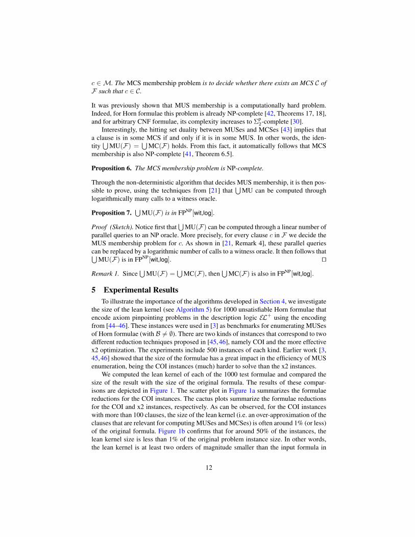
We computed the lean kernel of each of the 1000 test formulae and compared thesize of the result with the size of the original formula. The results of these compar-isons are depicted in Figure 1. The scatter plot in Figure 1a summarizes the formulaereductions for the COI instances. The cactus plots summarize the formulae reductionsfor the COI and x2 instances, respectively. As can be observed, for the COI instanceswith more than 100 clauses, the size of the lean kernel (i.e. an over-approximation of theclauses that are relevant for computing MUSes and MCSes) is often around 1% (or less)of the original formula. Figure 1b confirms that for around 50% of the instances, thelean kernel size is less than 1% of the original problem instance size. In other words,the lean kernel is at least two orders of magnitude smaller than the input formula in

12

100 101 102 103 104 105 106 107

lean kernel size, |K|

100

101

102

103

104

105

106

107

form

ula

size

,|F|

(a) Scatter plot for COI instances

0 100 200 300 400 500instances

10−3

10−2

10−1

100

101

102

|K|

|F|×

100

(%)

COI instances

(b) Cactus plot for COI instances

0 100 200 300 400 500instances

100

101

102

|K|

|F|×

100

(%)

x2 instances

(c) Cactus plot for x2 instances

Fig. 1: Formula reductions for COI and x2 instances

most of these cases. In practical terms, this means that for many of the Horn formulaeused for axiom pinpointing in the recent past based on COI reduction, around morethan 99% of the clauses are irrelevant for the computation of MUSes and MCSes. Theresults obtained for the x2 instances (Figure 1c) are not as dramatic. This was expectedas the x2 reduction is more effective in removing irrelevant clauses from the formula.However, even in this case the lean kernel is strictly smaller than the input formula in allbut 19 instances. From these 19 instances, one has 25 clauses, and all others contain 6clauses; thus, it is not surprising that no reduction was achieved through the lean kernel.Interestingly, about half of the instances observed a reduction of over 20%, and in someextreme cases the size of the formula was reduced in more than 90%. To the best ofour knowledge, these are the first practical problem instances for which the size of themaximum autarky (i.e., the complement of the lean kernel) is non-negligible.

6 ConclusionsWe have developed several new results related to reasoning about inconsistent Horn

formulae. These results complement earlier work [3, 5, 42], and find application in anumber of settings, including axiom pinpointing of lightweight description logics. Inparticular, we presented a polynomial delay algorithm for enumerating all MCSes, anda linear-time method for computing the lean kernel of a formula.

We illustrate the relevance of our work by analyzing Horn formulae that encode ax-iom pinpointing problems in the description logic EL+. The experimental results showthat commonly used Horn formulae [2, 3, 44] contain a very large proportion of irrel-evant clauses, i.e. clauses that do not interfere with consistency. With the exception ofa few outliers related with very small formulae, most formulae have around 99% ofirrelevant clauses, which can be identified with a linear time algorithm. From a prac-

13

tical perspective, a natural step is to exploit the linear time lean kernel identificationin state of the art axiom pinpointing tools [1–3, 32] and other problems where MUSenumeration and membership are important.

References1. M. F. Arif, C. Mencıa, A. Ignatiev, N. Manthey, R. Penaloza, and J. Marques-Silva. BEA-

CON: an efficient sat-based tool for debugging EL+ ontologies. In SAT, pages 521–530,2016.

2. M. F. Arif, C. Mencıa, and J. Marques-Silva. Efficient axiom pinpointing with EL2MCS. InKI, pages 225–233, 2015.

3. M. F. Arif, C. Mencıa, and J. Marques-Silva. Efficient MUS enumeration of Horn formulaewith applications to axiom pinpointing. In SAT, pages 324–342, 2015.

4. F. Baader, S. Brandt, and C. Lutz. Pushing the EL envelope. In IJCAI, pages 364–369, 2005.5. F. Baader, R. Penaloza, and B. Suntisrivaraporn. Pinpointing in the description logic EL+.

In KI, pages 52–67, 2007.6. F. Bacchus, J. Davies, M. Tsimpoukelli, and G. Katsirelos. Relaxation search: A simple way

of managing optional clauses. In AAAI, pages 835–841, 2014.7. F. Bacchus and G. Katsirelos. Using minimal correction sets to more efficiently compute

minimal unsatisfiable sets. In CAV, pages 70–86, 2015.8. R. R. Bakker, F. Dikker, F. Tempelman, and P. M. Wognum. Diagnosing and solving over-

determined constraint satisfaction problems. In IJCAI, pages 276–281, 1993.9. A. Bate, B. Motik, B. C. Grau, F. Simancik, and I. Horrocks. Extending consequence-based

reasoning to SRIQ. In KR, pages 187–196, 2016.10. A. Belov, I. Lynce, and J. Marques-Silva. Towards efficient MUS extraction. AI Commun.,

25(2):97–116, 2012.11. A. Biere, M. Heule, H. van Maaren, and T. Walsh, editors. Handbook of Satisfiability, volume

185 of Frontiers in Artificial Intelligence and Applications. IOS Press, 2009.12. N. Bjørner, F. Fioravanti, A. Rybalchenko, and V. Senni, editors. Proceedings First Workshop

on Horn Clauses for Verification and Synthesis, HCVS 2014, Vienna, Austria, 17 July 2014,volume 169 of EPTCS, 2014.

13. N. Bjørner, A. Gurfinkel, K. L. McMillan, and A. Rybalchenko. Horn clause solvers forprogram verification. In FoLC II, pages 24–51, 2015.

14. S. R. Buss, J. Krajıcek, and G. Takeuti. Provably total functions in the bounded arithmetictheories Ri

3, U i2, and V i

2 . In P. Clote and J. Krajıcek, editors, Arithmetic, Proof Theory, andComputational Complexity, pages 116–161. OUP, 1995.

15. J. W. Chinneck and E. W. Dravnieks. Locating minimal infeasible constraint sets in linearprograms. INFORMS Journal on Computing, 3(2):157–168, 1991.

16. W. F. Dowling and J. H. Gallier. Linear-time algorithms for testing the satisfiability of propo-sitional Horn formulae. J. Log. Program., 1(3):267–284, 1984.

17. T. Eiter and G. Gottlob. The complexity of logic-based abduction. J. ACM, 42(1):3–42,1995.

18. L. J. Henschen and L. Wos. Unit refutations and Horn sets. J. ACM, 21(4):590–605, 1974.19. A. Horn. On sentences which are true of direct unions of algebras. J. Symb. Log., 16(1):14–

21, 1951.20. A. Itai and J. A. Makowsky. Unification as a complexity measure for logic programming. J.

Log. Program., 4(2):105–117, 1987.21. M. Janota and J. Marques-Silva. On the query complexity of selecting minimal sets for

monotone predicates. Artif. Intell., 233:73–83, 2016.22. D. S. Johnson, C. H. Papadimitriou, and M. Yannakakis. On generating all maximal inde-

pendent sets. Inf. Process. Lett., 27(3):119–123, 1988.

14

23. Y. Kazakov, M. Krotzsch, and F. Simancik. The incredible ELK - from polynomial proce-dures to efficient reasoning with ontologies. J. Autom. Reasoning, 53(1):1–61, 2014.

24. H. Kleine Buning and O. Kullmann. Minimal unsatisfiability and autarkies. In Biere et al.[11], pages 339–401.

25. O. Kullmann. Investigations on autark assignments. Discrete Applied Mathematics, 107(1-3):99–137, 2000.

26. O. Kullmann. On the use of autarkies for satisfiability decision. Electronic Notes in DiscreteMathematics, 9:231–253, 2001.

27. O. Kullmann, I. Lynce, and J. Marques-Silva. Categorisation of clauses in conjunctive nor-mal forms: Minimally unsatisfiable sub-clause-sets and the lean kernel. In SAT, pages 22–35,2006.

28. O. Kullmann and J. Marques-Silva. Computing maximal autarkies with few and simpleoracle queries. In SAT, pages 138–155, 2015.

29. C. M. Li, F. Manya, N. O. Mohamedou, and J. Planes. Resolution-based lower bounds inMaxSAT. Constraints, 15(4):456–484, 2010.

30. P. Liberatore. Redundancy in logic I: CNF propositional formulae. Artif. Intell., 163(2):203–232, 2005.

31. P. Liberatore. Redundancy in logic II: 2CNF and Horn propositional formulae. Artif. Intell.,172(2-3):265–299, 2008.

32. N. Manthey, R. Penaloza, and S. Rudolph. Efficient axiom pinpointing in EL using SATtechnology. In DL, 2016.

33. J. Marques-Silva, F. Heras, M. Janota, A. Previti, and A. Belov. On computing minimalcorrection subsets. In IJCAI, pages 615–622, 2013.

34. J. Marques-Silva, A. Ignatiev, A. Morgado, V. M. Manquinho, and I. Lynce. Efficient au-tarkies. In ECAI, pages 603–608, 2014.

35. C. Mencıa, A. Ignatiev, A. Previti, and J. Marques-Silva. MCS extraction with sublinearoracle queries. In SAT, pages 342–360, 2016.

36. C. Mencıa, A. Previti, and J. Marques-Silva. Literal-based MCS extraction. In IJCAI, pages1973–1979, 2015.

37. M. Minoux. LTUR: A simplified linear-time unit resolution algorithm for Horn formulaeand computer implementation. Inf. Process. Lett., 29(1):1–12, 1988.

38. B. Monien and E. Speckenmeyer. Solving satisfiability in less than 2n steps. Discrete AppliedMathematics, 10(3):287–295, 1985.

39. C. H. Papadimitriou. Computational Complexity. Addison Wesley, 1993.40. C. H. Papadimitriou. NP-completeness: A retrospective. In ICALP, pages 2–6, 1997.41. R. Penaloza. Axiom-Pinpointing in Description Logics and Beyond. PhD thesis, Dresden

University of Technology, Germany, 2009.42. R. Penaloza and B. Sertkaya. On the complexity of axiom pinpointing in the EL family of

description logics. In KR, 2010.43. R. Reiter. A theory of diagnosis from first principles. Artif. Intell., 32(1):57–95, 1987.44. R. Sebastiani and M. Vescovi. Axiom pinpointing in lightweight description logics via Horn-

SAT encoding and conflict analysis. In CADE, pages 84–99, 2009.45. R. Sebastiani and M. Vescovi. Axiom pinpointing in large EL+ ontologies via SAT and SMT

techniques. Technical Report DISI-15-010, DISI, University of Trento, Italy, April 2015.Available as http://disi.unitn.it/˜rseba/elsat/elsat_techrep.pdf.

46. M. Vescovi. Exploiting SAT and SMT Techniques for Automated Reasoning and OntologyManipulation in Description Logics. PhD thesis, University of Trento, 2011.

15