Efficient and Robust Automated Machine Learning

Matthias Feurer Aaron Klein Katharina EggenspergerJost Tobias Springenberg Manuel Blum Frank Hutter

Department of Computer ScienceUniversity of Freiburg, Germany

{feurerm,kleinaa,eggenspk,springj,mblum,fh}@cs.uni-freiburg.de

Abstract

The success of machine learning in a broad range of applications has led to anever-growing demand for machine learning systems that can be used off the shelfby non-experts. To be effective in practice, such systems need to automaticallychoose a good algorithm and feature preprocessing steps for a new dataset at hand,and also set their respective hyperparameters. Recent work has started to tackle thisautomated machine learning (AutoML) problem with the help of efficient Bayesianoptimization methods. In this work we introduce a robust new AutoML systembased on scikit-learn (using 15 classifiers, 14 feature preprocessing methods, and 4data preprocessing methods, giving rise to a structured hypothesis space with 110hyperparameters). This system, which we dub auto-sklearn, improves on existingAutoML methods by automatically taking into account past performance on similardatasets, and by constructing ensembles from the models evaluated during theoptimization. Our system won the first phase of the ongoing ChaLearn AutoMLchallenge, and our comprehensive analysis on over 100 diverse datasets showsthat it substantially outperforms the previous state of the art in AutoML. We alsodemonstrate the performance gains due to each of our contributions and deriveinsights into the effectiveness of the individual components of auto-sklearn.

1 Introduction

Machine learning has recently made great strides in many application areas, fueling a growingdemand for machine learning systems that can be used effectively by novices in machine learning.Correspondingly, a growing number of commercial enterprises aim to satisfy this demand (e.g.,BigML.com, Wise.io, SkyTree.com, RapidMiner.com, Dato.com, Prediction.io, DataRobot.com, Mi-crosoft’s Azure Machine Learning, Google’s Prediction API, and Amazon Machine Learning). At itscore, every effective machine learning service needs to solve the fundamental problems of decidingwhich machine learning algorithm to use on a given dataset, whether and how to preprocess itsfeatures, and how to set all hyperparameters. This is the problem we address in this work.

We define AutoML as the problem of automatically (without human input) producing test setpredictions for a new dataset within a fixed computational budget. More formally, we study thefollowing AutoML problem:

Definition 1 (AutoML). For i = 1, . . . , n + m, let xi ∈ Rd denote a feature vector and yi ∈ Ythe corresponding target value. Given a training dataset Dtrain = {(x1, y1), . . . , (xn, yn)} andthe feature vectors xn+1, . . . ,xn+m of a test dataset Dtest = {(xn+1, yn+1), . . . , (xn+m, yn+m)}drawn from the same underlying data distribution, as well as a resource budget b and a loss metricL(·, ·), the AutoML problem is to (automatically) produce test set predictions yn+1, . . . , yn+m. Theloss of a solution yn+1, . . . , yn+m to the AutoML problem is given by 1

m

∑mj=1 L(yn+j , yn+j).

1

In practice, the budget b would comprise computational resources, such as CPU and/or wallclock timeand memory usage. This problem definition reflects the setting of the ongoing ChaLearn AutoMLchallenge [1]. The AutoML system we describe here won the first phase of that challenge.

Our approach to the AutoML problem is motivated by Auto-WEKA [2], which combines the machinelearning framework WEKA [3] with a Bayesian optimization [4] method for selecting a goodinstantiation of WEKA for a given dataset. Section 2 describes this approach in more detail.

The contribution of this paper is to extend this approach in various ways that considerably improveits efficiency and robustness, based on principles that apply to a wide range of machine learningframeworks (such as those used by the machine learning service providers mentioned above). First,following successful previous work for low dimensional optimization problems [5, 6, 7], we reasonacross datasets to identify instantiations of machine learning frameworks that perform well on a newdataset and warmstart Bayesian optimization with them (Section 3.1). Second, we automaticallyconstruct ensembles of the models considered by Bayesian optimization (Section 3.2). Third,we carefully design a highly parameterized machine learning framework from high-performingclassifiers and preprocessors implemented in the popular machine learning framework scikit-learn [8](Section 4). Finally, we perform an extensive empirical analysis using a diverse collection ofdatasets to demonstrate that the resulting auto-sklearn system outperforms previous state-of-the-artAutoML methods (Section 5), to show that each of our contributions leads to substantial performanceimprovements (Section 6), and to gain insights into the performance of the individual classifiers andpreprocessors used in auto-sklearn (Section 7).

2 AutoML as a CASH problem

We first briefly review existing mechanisms for automated machine learning and its formalization asa Combined Algorithm Selection and Hyperparameter optimization (CASH) problem. Two importantproblems in AutoML are that (1) no single machine learning method performs best on all datasetsand (2) some machine learning methods (e.g., non-linear SVMs) crucially rely on hyperparameteroptimization. The latter problem has been successfully attacked using Bayesian optimization [4],which nowadays forms a core component of an AutoML system. The former problem is intertwinedwith the latter since the rankings of algorithms depend on whether their hyperparameters are tunedproperly. Fortunately, the two problems can efficiently be tackled as a single, structured, jointoptimization problem:

Definition 2 (CASH). LetA = {A(1), . . . , A(R)} be a set of algorithms, and let the hyperparametersof each algorithm A(j) have domain Λ(j). Further, let Dtrain = {(x1, y1), . . . , (xn, yn)} be a train-ing set which is split into K cross-validation folds {D(1)

valid, . . . , D(K)valid} and {D(1)

train, . . . , D(K)train}

such that D(i)train = Dtrain\D(i)

valid for i = 1, . . . ,K. Finally, let L(A(j)λ , D

(i)train, D

(i)valid) denote the

loss that algorithm A(j) achieves on D(i)valid when trained on D

(i)train with hyperparameters λ. Then,

the Combined Algorithm Selection and Hyperparameter optimization (CASH) problem is to find thejoint algorithm and hyperparameter setting that minimizes this loss:

A?,λ? ∈ argminA(j)∈A,λ∈Λ(j)

1

K

K∑i=1

L(A(j)λ , D

(i)train, D

(i)valid). (1)

This CASH problem was first tackled by Thornton et al. [2] in the Auto-WEKA system usingtree-based Bayesian optimization methods [9, 10]. In a nutshell, Bayesian optimization [4] fits aprobabilistic model to capture the relationship between hyperparameter settings and their measuredperformance; it then uses this model to select the most promising hyperparameter setting (tradingoff exploration of new parts of the space vs. exploitation in known good regions), evaluates thathyperparameter setting, updates the model with the result, and iterates. While Bayesian optimizationbased on Gaussian process models (e.g., Snoek et al. [11]) performs best in low-dimensional problemswith numerical hyperparameters, tree-based models have been shown to be more successful in high-dimensional, structured, and partly discrete problems [12] – such as the CASH problem – and are alsoused in the AutoML framework hyperopt-sklearn [13]. Among the tree-based Bayesian optimizationmethods, Thornton et al. [2] found the random-forest-based SMAC [9] to outperform the tree Parzenestimator TPE [10], and we therefore use SMAC to solve the CASH problem in this paper. Next to its

2

AutoMLsystem

ML framework

{Xtrain, Ytrain,Xtest, b,L}

meta-learning

data pre-processor

featurepreprocessor

classifierbuild

ensembleYtest

Bayesian optimizer

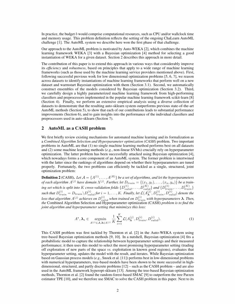
Figure 1: Our improved approach to AutoML. We add two components to Bayesian hyperparameter optimizationof an ML framework: meta-learning for initializing the Bayesian optimizer and automated ensemble constructionfrom configurations evaluated during optimization.

use of random forests [14], SMAC’s main distinguishing feature is that it allows fast cross-validationby evaluating one fold at a time and discarding poorly-performing hyperparameter settings early.

3 New methods for increasing efficiency and robustness of AutoML

We now discuss our two improvements to the basic CASH formulation of AutoML. First, we includea meta-learning step in the AutoML pipeline to warmstart the Bayesian optimization procedure,which results in a considerable boost in the efficiency of the system. Second, we include an automatedensemble construction step, allowing us to use all classifiers that were found by Bayesian optimization.

Figure 1 summarizes the overall workflow of an AutoML system including both of our improvements.We note that we expect their effectiveness to be greater for flexible ML frameworks that offer manydegrees of freedom (e.g., many algorithms, hyperparameters, and preprocessing methods).

3.1 Meta-learning for finding good instantiations of machine learning frameworks

Domain experts derive knowledge from previous tasks: They learn about the performance of machinelearning algorithms. The area of meta-learning [15] mimics this strategy by reasoning about theperformance of learning algorithms across datasets. In this work, we apply meta-learning to selectinstantiations of our given machine learning framework that are likely to perform well on a newdataset. More specifically, for a large number of datasets, we collect both performance data and a setof meta-features, i.e., characteristics of the dataset that can be computed efficiently and that help usdetermine which algorithm to use on a new dataset.

This meta-learning approach is complementary to Bayesian optimization for optimizing an MLframework. Meta-learning can quickly suggest some instantiations of the ML framework that arelikely to perform quite well, but it is unable to provide fine-grained information on performance.In contrast, Bayesian optimization is slow to start for hyperparameter spaces as large as those ofentire ML frameworks, but can fine-tune performance over time. We exploit this complementarity byselecting k configurations based on meta-learning and use their result to seed Bayesian optimization.This approach of warmstarting optimization by meta-learning has already been successfully appliedbefore [5, 6, 7], but never to an optimization problem as complex as that of searching the spaceof instantiations of a full-fledged ML framework. Likewise, learning across datasets has alsobeen applied in collaborative Bayesian optimization methods [16, 17]; while these approaches arepromising, they are so far limited to very few meta-features and cannot yet cope with the high-dimensional partially discrete configuration spaces faced in AutoML.

More precisely, our meta-learning approach works as follows. In an offline phase, for each machinelearning dataset in a dataset repository (in our case 140 datasets from the OpenML [18] repository),we evaluated a set of meta-features (described below) and used Bayesian optimization to determineand store an instantiation of the given ML framework with strong empirical performance for thatdataset. (In detail, we ran SMAC [9] for 24 hours with 10-fold cross-validation on two thirds of thedata and stored the resulting ML framework instantiation which exhibited best performance on theremaining third). Then, given a new dataset D, we compute its meta-features, rank all datasets bytheir L1 distance to D in meta-feature space and select the stored ML framework instantiations forthe k = 25 nearest datasets for evaluation before starting Bayesian optimization with their results.

To characterize datasets, we implemented a total of 38 meta-features from the literature, includingsimple, information-theoretic and statistical meta-features [19, 20], such as statistics about the numberof data points, features, and the number of classes, or data skewness, and the entropy of the targets.All meta-features are listed in Table 1 of the supplementary material. Notably, we had to exclude the

3

prominent and effective category of landmarking meta-features [21] (which measure the performanceof simple base learners), because they were computationally too expensive to be helpful in the onlineevaluation phase. We note that this meta-learning approach draws its power from the availability ofa repository of datasets; due to recent initiatives, such as OpenML [18], we expect the number ofavailable datasets to grow ever larger over time, increasing the importance of meta-learning.

3.2 Automated ensemble construction of models evaluated during optimization

While Bayesian hyperparameter optimization is data-efficient in finding the best-performing hyperpa-rameter setting, we note that it is a very wasteful procedure when the goal is simply to make goodpredictions: all the models it trains during the course of the search are lost, usually including somethat perform almost as well as the best. Rather than discarding these models, we propose to store themand to use an efficient post-processing method (which can be run in a second process on-the-fly) toconstruct an ensemble out of them. This automatic ensemble construction avoids to commit itself to asingle hyperparameter setting and is thus more robust (and less prone to overfitting) than using thepoint estimate that standard hyperparameter optimization yields. To our best knowledge, we are thefirst to make this simple observation, which can be applied to improve any Bayesian hyperparameteroptimization method.

It is well known that ensembles often outperform individual models [22, 23], and that effectiveensembles can be created from a library of models [24, 25]. Ensembles perform particularly well ifthe models they are based on (1) are individually strong and (2) make uncorrelated errors [14]. Sincethis is much more likely when the individual models are different in nature, ensemble building isparticularly well suited for combining strong instantiations of a flexible ML framework.

However, simply building a uniformly weighted ensemble of the models found by Bayesian optimiza-tion does not work well. Rather, we found it crucial to adjust these weights using the predictions ofall individual models on a hold-out set. We experimented with different approaches to optimize theseweights: stacking [26], gradient-free numerical optimization, and the method ensemble selection [24].While we found both numerical optimization and stacking to overfit to the validation set and to becomputationally costly, ensemble selection was fast and robust. We therefore used this technique inall experiments – building an ensemble of size 50 out of the 50 best models. In a nutshell, ensembleselection (introduced by Caruana et al. [24]) is a greedy procedure that starts from an empty ensembleand then iteratively adds the model that maximizes ensemble validation performance (with uniformweight, but allowing for repetitions). Procedure 1 in the supplementary material describes it in detail.

4 A practical automated machine learning system

datapreprocessor

estimatorfeaturepreprocessor classifier

AdaBoost· · ·RF kNN

# estimatorslearning rate max. depth

preprocessing

· · ·NonePCA fast ICA

rescaling

· · ·min/max standard

one hot enc.

· · ·

imputation

mean · · · median

balancing

weighting None

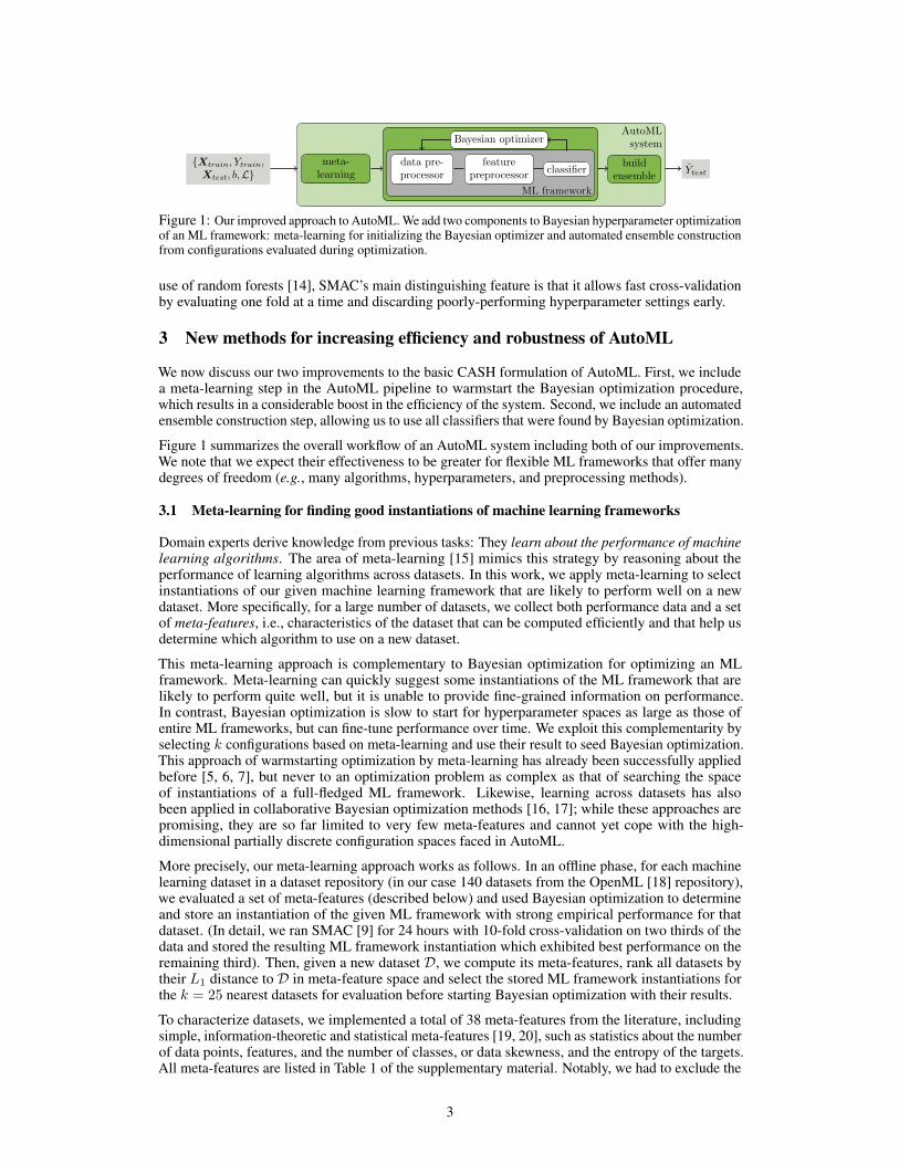
Figure 2: Structured configuration space. Squared boxesdenote parent hyperparameters whereas boxes with roundededges are leaf hyperparameters. Grey colored boxes markactive hyperparameters which form an example configurationand machine learning pipeline. Each pipeline comprises onefeature preprocessor, classifier and up to three data prepro-cessor methods plus respective hyperparameters.

To design a robust AutoML system, asour underlying ML framework we chosescikit-learn [8], one of the best knownand most widely used machine learninglibraries. It offers a wide range of well es-tablished and efficiently-implemented MLalgorithms and is easy to use for both ex-perts and beginners. Due to its relationshipto scikit-learn, we dub our resulting Au-toML system auto-sklearn.

Figure 2 depicts auto-sklearn’s overall com-ponents. It comprises 15 classification al-gorithms, 14 preprocessing methods, and 4data preprocessing methods. We parameter-ized each of them which resulted in a spaceof 110 hyperparameters. Most of them areconditional hyperparameters that are only active if their respective component is selected. We notethat SMAC [9] can handle this conditionality natively.

All 15 classification algorithms in auto-sklearn are depicted in Table 1a. They fall into differentcategories, such as general linear models (2 algorithms), support vector machines (2), discriminant

4

name #λ cat (cond) cont (cond)

AdaBoost (AB) 4 1 (-) 3 (-)Bernoulli naıve Bayes 2 1 (-) 1 (-)decision tree (DT) 4 1 (-) 3 (-)extreml. rand. trees 5 2 (-) 3 (-)Gaussian naıve Bayes - - -gradient boosting (GB) 6 - 6 (-)kNN 3 2 (-) 1 (-)LDA 4 1 (-) 3 (1)linear SVM 4 2 (-) 2 (-)kernel SVM 7 2 (-) 5 (2)multinomial naıve Bayes 2 1 (-) 1 (-)passive aggressive 3 1 (-) 2 (-)QDA 2 - 2 (-)random forest (RF) 5 2 (-) 3 (-)Linear Class. (SGD) 10 4 (-) 6 (3)

(a) classification algorithms

name #λ cat (cond) cont (cond)

extreml. rand. trees prepr. 5 2 (-) 3 (-)fast ICA 4 3 (-) 1 (1)feature agglomeration 4 3 () 1 (-)kernel PCA 5 1 (-) 4 (3)rand. kitchen sinks 2 - 2 (-)linear SVM prepr. 3 1 (-) 2 (-)no preprocessing - - -nystroem sampler 5 1 (-) 4 (3)PCA 2 1 (-) 1 (-)polynomial 3 2 (-) 1 (-)random trees embed. 4 - 4 (-)select percentile 2 1 (-) 1 (-)select rates 3 2 (-) 1 (-)

one-hot encoding 2 1 (-) 1 (1)imputation 1 1 (-) -balancing 1 1 (-) -rescaling 1 1 (-) -

(b) preprocessing methods

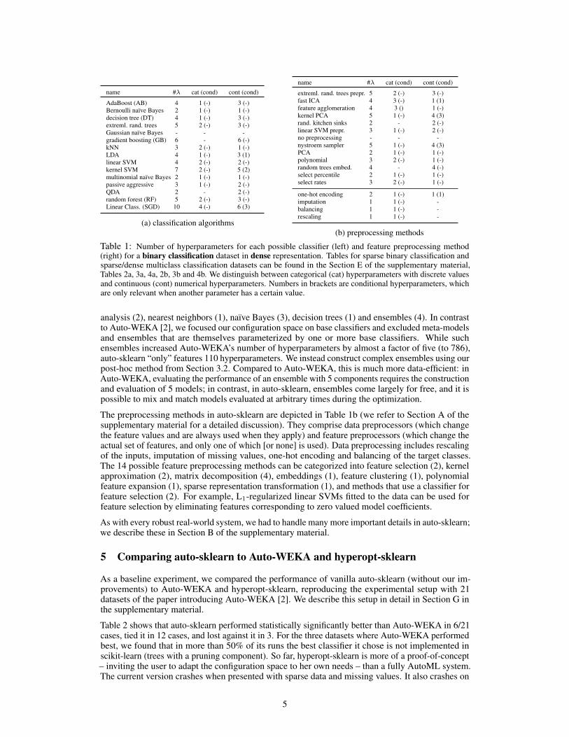
Table 1: Number of hyperparameters for each possible classifier (left) and feature preprocessing method(right) for a binary classification dataset in dense representation. Tables for sparse binary classification andsparse/dense multiclass classification datasets can be found in the Section E of the supplementary material,Tables 2a, 3a, 4a, 2b, 3b and 4b. We distinguish between categorical (cat) hyperparameters with discrete valuesand continuous (cont) numerical hyperparameters. Numbers in brackets are conditional hyperparameters, whichare only relevant when another parameter has a certain value.

analysis (2), nearest neighbors (1), naıve Bayes (3), decision trees (1) and ensembles (4). In contrastto Auto-WEKA [2], we focused our configuration space on base classifiers and excluded meta-modelsand ensembles that are themselves parameterized by one or more base classifiers. While suchensembles increased Auto-WEKA’s number of hyperparameters by almost a factor of five (to 786),auto-sklearn “only” features 110 hyperparameters. We instead construct complex ensembles using ourpost-hoc method from Section 3.2. Compared to Auto-WEKA, this is much more data-efficient: inAuto-WEKA, evaluating the performance of an ensemble with 5 components requires the constructionand evaluation of 5 models; in contrast, in auto-sklearn, ensembles come largely for free, and it ispossible to mix and match models evaluated at arbitrary times during the optimization.

The preprocessing methods in auto-sklearn are depicted in Table 1b (we refer to Section A of thesupplementary material for a detailed discussion). They comprise data preprocessors (which changethe feature values and are always used when they apply) and feature preprocessors (which change theactual set of features, and only one of which [or none] is used). Data preprocessing includes rescalingof the inputs, imputation of missing values, one-hot encoding and balancing of the target classes.The 14 possible feature preprocessing methods can be categorized into feature selection (2), kernelapproximation (2), matrix decomposition (4), embeddings (1), feature clustering (1), polynomialfeature expansion (1), sparse representation transformation (1), and methods that use a classifier forfeature selection (2). For example, L1-regularized linear SVMs fitted to the data can be used forfeature selection by eliminating features corresponding to zero valued model coefficients.

As with every robust real-world system, we had to handle many more important details in auto-sklearn;we describe these in Section B of the supplementary material.

5 Comparing auto-sklearn to Auto-WEKA and hyperopt-sklearn

As a baseline experiment, we compared the performance of vanilla auto-sklearn (without our im-provements) to Auto-WEKA and hyperopt-sklearn, reproducing the experimental setup with 21datasets of the paper introducing Auto-WEKA [2]. We describe this setup in detail in Section G inthe supplementary material.

Table 2 shows that auto-sklearn performed statistically significantly better than Auto-WEKA in 6/21cases, tied it in 12 cases, and lost against it in 3. For the three datasets where Auto-WEKA performedbest, we found that in more than 50% of its runs the best classifier it chose is not implemented inscikit-learn (trees with a pruning component). So far, hyperopt-sklearn is more of a proof-of-concept– inviting the user to adapt the configuration space to her own needs – than a fully AutoML system.The current version crashes when presented with sparse data and missing values. It also crashes on

5

Aba

lone

Am

azon

Car

Cifa

r-10

Cifa

r-10

Smal

l

Con

vex

Dex

ter

Dor

othe

a

Ger

man

Cre

dit

Gis

ette

KD

D09

App

eten

cy

KR

-vs-

KP

Mad

elon

MN

IST

Bas

ic

MR

BI

Seco

m

Sem

eion

Shut

tle

Wav

efor

m

Win

eQ

ualit

y

Yea

st

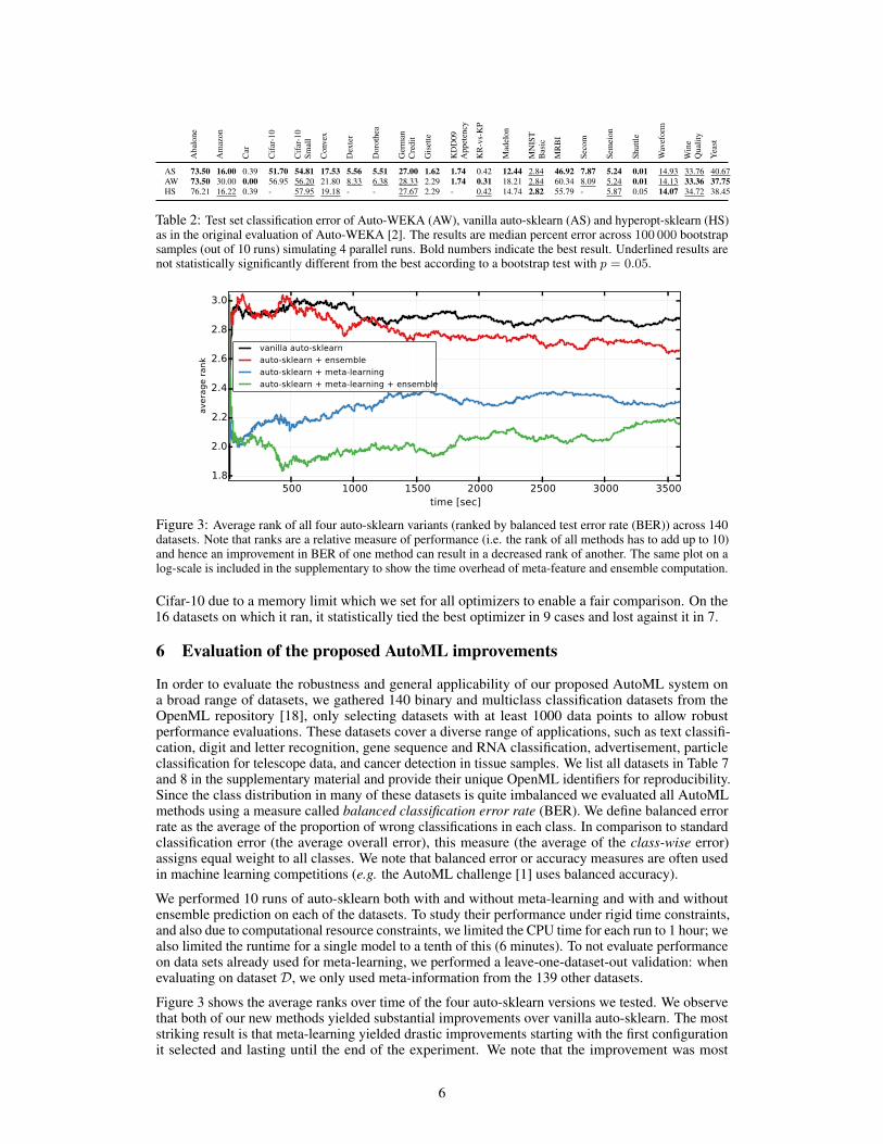
AS 73.50 16.00 0.39 51.70 54.81 17.53 5.56 5.51 27.00 1.62 1.74 0.42 12.44 2.84 46.92 7.87 5.24 0.01 14.93 33.76 40.67AW 73.50 30.00 0.00 56.95 56.20 21.80 8.33 6.38 28.33 2.29 1.74 0.31 18.21 2.84 60.34 8.09 5.24 0.01 14.13 33.36 37.75HS 76.21 16.22 0.39 - 57.95 19.18 - - 27.67 2.29 - 0.42 14.74 2.82 55.79 - 5.87 0.05 14.07 34.72 38.45

Table 2: Test set classification error of Auto-WEKA (AW), vanilla auto-sklearn (AS) and hyperopt-sklearn (HS)as in the original evaluation of Auto-WEKA [2]. The results are median percent error across 100 000 bootstrapsamples (out of 10 runs) simulating 4 parallel runs. Bold numbers indicate the best result. Underlined results arenot statistically significantly different from the best according to a bootstrap test with p = 0.05.

500 1000 1500 2000 2500 3000 3500time [sec]

1.8

2.0

2.2

2.4

2.6

2.8

3.0

avera

ge r

ank

vanilla auto-sklearn

auto-sklearn + ensemble

auto-sklearn + meta-learning

auto-sklearn + meta-learning + ensemble

Figure 3: Average rank of all four auto-sklearn variants (ranked by balanced test error rate (BER)) across 140datasets. Note that ranks are a relative measure of performance (i.e. the rank of all methods has to add up to 10)and hence an improvement in BER of one method can result in a decreased rank of another. The same plot on alog-scale is included in the supplementary to show the time overhead of meta-feature and ensemble computation.

Cifar-10 due to a memory limit which we set for all optimizers to enable a fair comparison. On the16 datasets on which it ran, it statistically tied the best optimizer in 9 cases and lost against it in 7.

6 Evaluation of the proposed AutoML improvements

In order to evaluate the robustness and general applicability of our proposed AutoML system ona broad range of datasets, we gathered 140 binary and multiclass classification datasets from theOpenML repository [18], only selecting datasets with at least 1000 data points to allow robustperformance evaluations. These datasets cover a diverse range of applications, such as text classifi-cation, digit and letter recognition, gene sequence and RNA classification, advertisement, particleclassification for telescope data, and cancer detection in tissue samples. We list all datasets in Table 7and 8 in the supplementary material and provide their unique OpenML identifiers for reproducibility.Since the class distribution in many of these datasets is quite imbalanced we evaluated all AutoMLmethods using a measure called balanced classification error rate (BER). We define balanced errorrate as the average of the proportion of wrong classifications in each class. In comparison to standardclassification error (the average overall error), this measure (the average of the class-wise error)assigns equal weight to all classes. We note that balanced error or accuracy measures are often usedin machine learning competitions (e.g. the AutoML challenge [1] uses balanced accuracy).

We performed 10 runs of auto-sklearn both with and without meta-learning and with and withoutensemble prediction on each of the datasets. To study their performance under rigid time constraints,and also due to computational resource constraints, we limited the CPU time for each run to 1 hour; wealso limited the runtime for a single model to a tenth of this (6 minutes). To not evaluate performanceon data sets already used for meta-learning, we performed a leave-one-dataset-out validation: whenevaluating on dataset D, we only used meta-information from the 139 other datasets.

Figure 3 shows the average ranks over time of the four auto-sklearn versions we tested. We observethat both of our new methods yielded substantial improvements over vanilla auto-sklearn. The moststriking result is that meta-learning yielded drastic improvements starting with the first configurationit selected and lasting until the end of the experiment. We note that the improvement was most

6

Ope

nML

data

setI

D

auto

-skl

earn

Ada

Boo

st

Ber

noul

lina

ıve

Bay

es

deci

sion

tree

extr

eml.

rand

.tre

es

Gau

ssia

nna

ıve

Bay

es

grad

ient

boos

ting

kNN

LD

A

linea

rSV

M

kern

elSV

M

mul

tinom

ial

naıv

eB

ayes

pass

ive

aggr

esiv

e

QD

A

rand

omfo

rest

Lin

earC

lass

.(S

GD

)

38 2.15 2.68 50.22 2.15 18.06 11.22 1.77 50.00 8.55 16.29 17.89 46.99 50.00 8.78 2.34 15.8246 3.76 4.65 - 5.62 4.74 7.88 3.49 7.57 8.67 8.31 5.36 7.55 9.23 7.57 4.20 7.31

179 16.99 17.03 19.27 18.31 17.09 21.77 17.00 22.23 18.93 17.30 17.57 18.97 22.29 19.06 17.24 17.01184 10.32 10.52 - 17.46 11.10 64.74 10.42 31.10 35.44 15.76 12.52 27.13 20.01 47.18 10.98 12.76554 1.55 2.42 - 12.00 2.91 10.52 3.86 2.68 3.34 2.23 1.50 10.37 100.00 2.75 3.08 2.50772 46.85 49.68 47.90 47.75 45.62 48.83 48.15 48.00 46.74 48.38 48.66 47.21 48.75 47.67 47.71 47.93917 10.22 9.11 25.83 11.00 10.22 33.94 10.11 11.11 34.22 18.67 6.78 25.50 20.67 30.44 10.83 18.33

1049 12.93 12.53 15.50 19.31 17.18 26.23 13.38 23.80 25.12 17.28 21.44 26.40 29.25 21.38 13.75 19.921111 23.70 23.16 28.40 24.40 24.47 29.59 22.93 50.30 24.11 23.99 23.56 27.67 43.79 25.86 28.06 23.361120 13.81 13.54 18.81 17.45 13.86 21.50 13.61 17.23 15.48 14.94 14.17 18.33 16.37 15.62 13.70 14.661128 4.21 4.89 4.71 9.30 3.89 4.77 4.58 4.59 4.58 4.83 4.59 4.46 5.65 5.59 3.83 4.33293 2.86 4.07 24.30 5.03 3.59 32.44 24.48 4.86 24.40 14.16 100.00 24.20 21.34 28.68 2.57 15.54389 19.65 22.98 - 33.14 19.38 29.18 19.20 30.87 19.68 17.95 22.04 20.04 20.14 39.57 20.66 17.99

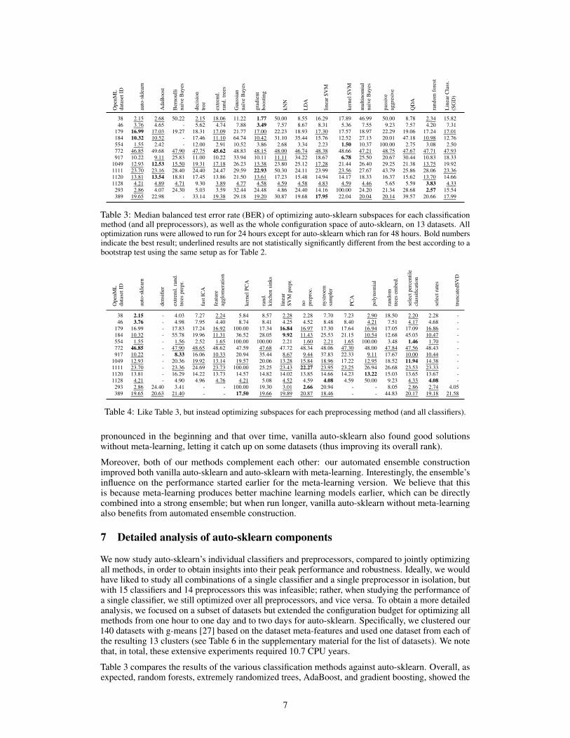
Table 3: Median balanced test error rate (BER) of optimizing auto-sklearn subspaces for each classificationmethod (and all preprocessors), as well as the whole configuration space of auto-sklearn, on 13 datasets. Alloptimization runs were allowed to run for 24 hours except for auto-sklearn which ran for 48 hours. Bold numbersindicate the best result; underlined results are not statistically significantly different from the best according to abootstrap test using the same setup as for Table 2.

Ope

nML

data

setI

D

auto

-skl

earn

dens

ifier

extr

eml.

rand

.tr

ees

prep

r.

fast

ICA

feat

ure

aggl

omer

atio

n

kern

elPC

A

rand

.ki

tche

nsi

nks

linea

rSV

Mpr

epr.

no prep

roc.

nyst

roem

sam

pler

PCA

poly

nom

ial

rand

omtr

ees

embe

d.

sele

ctpe

rcen

tile

clas

sific

atio

n

sele

ctra

tes

trun

cate

dSV

D

38 2.15 - 4.03 7.27 2.24 5.84 8.57 2.28 2.28 7.70 7.23 2.90 18.50 2.20 2.28 -46 3.76 - 4.98 7.95 4.40 8.74 8.41 4.25 4.52 8.48 8.40 4.21 7.51 4.17 4.68 -

179 16.99 - 17.83 17.24 16.92 100.00 17.34 16.84 16.97 17.30 17.64 16.94 17.05 17.09 16.86 -184 10.32 - 55.78 19.96 11.31 36.52 28.05 9.92 11.43 25.53 21.15 10.54 12.68 45.03 10.47 -554 1.55 - 1.56 2.52 1.65 100.00 100.00 2.21 1.60 2.21 1.65 100.00 3.48 1.46 1.70 -772 46.85 - 47.90 48.65 48.62 47.59 47.68 47.72 48.34 48.06 47.30 48.00 47.84 47.56 48.43 -917 10.22 - 8.33 16.06 10.33 20.94 35.44 8.67 9.44 37.83 22.33 9.11 17.67 10.00 10.44 -

1049 12.93 - 20.36 19.92 13.14 19.57 20.06 13.28 15.84 18.96 17.22 12.95 18.52 11.94 14.38 -1111 23.70 - 23.36 24.69 23.73 100.00 25.25 23.43 22.27 23.95 23.25 26.94 26.68 23.53 23.33 -1120 13.81 - 16.29 14.22 13.73 14.57 14.82 14.02 13.85 14.66 14.23 13.22 15.03 13.65 13.67 -1128 4.21 - 4.90 4.96 4.76 4.21 5.08 4.52 4.59 4.08 4.59 50.00 9.23 4.33 4.08 -293 2.86 24.40 3.41 - - 100.00 19.30 3.01 2.66 20.94 - - 8.05 2.86 2.74 4.05389 19.65 20.63 21.40 - - 17.50 19.66 19.89 20.87 18.46 - - 44.83 20.17 19.18 21.58

Table 4: Like Table 3, but instead optimizing subspaces for each preprocessing method (and all classifiers).

pronounced in the beginning and that over time, vanilla auto-sklearn also found good solutionswithout meta-learning, letting it catch up on some datasets (thus improving its overall rank).

Moreover, both of our methods complement each other: our automated ensemble constructionimproved both vanilla auto-sklearn and auto-sklearn with meta-learning. Interestingly, the ensemble’sinfluence on the performance started earlier for the meta-learning version. We believe that thisis because meta-learning produces better machine learning models earlier, which can be directlycombined into a strong ensemble; but when run longer, vanilla auto-sklearn without meta-learningalso benefits from automated ensemble construction.

7 Detailed analysis of auto-sklearn components

We now study auto-sklearn’s individual classifiers and preprocessors, compared to jointly optimizingall methods, in order to obtain insights into their peak performance and robustness. Ideally, we wouldhave liked to study all combinations of a single classifier and a single preprocessor in isolation, butwith 15 classifiers and 14 preprocessors this was infeasible; rather, when studying the performance ofa single classifier, we still optimized over all preprocessors, and vice versa. To obtain a more detailedanalysis, we focused on a subset of datasets but extended the configuration budget for optimizing allmethods from one hour to one day and to two days for auto-sklearn. Specifically, we clustered our140 datasets with g-means [27] based on the dataset meta-features and used one dataset from each ofthe resulting 13 clusters (see Table 6 in the supplementary material for the list of datasets). We notethat, in total, these extensive experiments required 10.7 CPU years.

Table 3 compares the results of the various classification methods against auto-sklearn. Overall, asexpected, random forests, extremely randomized trees, AdaBoost, and gradient boosting, showed the

7

101 102 103 104

time [sec]

0

2

4

6

8

10

Bala

nce

d E

rror

Rate

auto-sklearn

gradient boosting

kernel SVM

random forest

(a) MNIST (OpenML dataset ID 554)

101 102 103 104

time [sec]

15

20

25

30

35

40

45

50

Bala

nce

d E

rror

Rate

auto-sklearn

gradient boosting

kernel SVM

random forest

(b) Promise pc4 (OpenML dataset ID 1049)

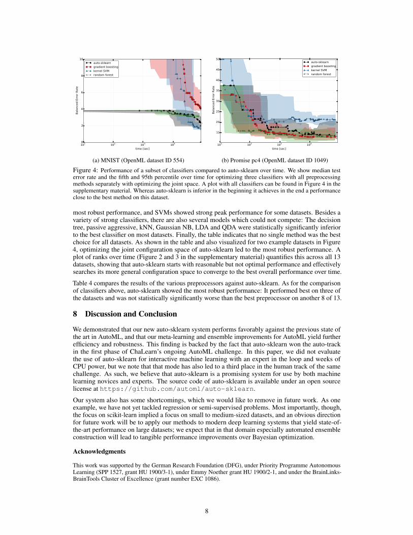
Figure 4: Performance of a subset of classifiers compared to auto-sklearn over time. We show median testerror rate and the fifth and 95th percentile over time for optimizing three classifiers with all preprocessingmethods separately with optimizing the joint space. A plot with all classifiers can be found in Figure 4 in thesupplementary material. Whereas auto-sklearn is inferior in the beginning it achieves in the end a performanceclose to the best method on this dataset.

most robust performance, and SVMs showed strong peak performance for some datasets. Besides avariety of strong classifiers, there are also several models which could not compete: The decisiontree, passive aggressive, kNN, Gaussian NB, LDA and QDA were statistically significantly inferiorto the best classifier on most datasets. Finally, the table indicates that no single method was the bestchoice for all datasets. As shown in the table and also visualized for two example datasets in Figure4, optimizing the joint configuration space of auto-sklearn led to the most robust performance. Aplot of ranks over time (Figure 2 and 3 in the supplementary material) quantifies this across all 13datasets, showing that auto-sklearn starts with reasonable but not optimal performance and effectivelysearches its more general configuration space to converge to the best overall performance over time.

Table 4 compares the results of the various preprocessors against auto-sklearn. As for the comparisonof classifiers above, auto-sklearn showed the most robust performance: It performed best on three ofthe datasets and was not statistically significantly worse than the best preprocessor on another 8 of 13.

8 Discussion and Conclusion

We demonstrated that our new auto-sklearn system performs favorably against the previous state ofthe art in AutoML, and that our meta-learning and ensemble improvements for AutoML yield furtherefficiency and robustness. This finding is backed by the fact that auto-sklearn won the auto-trackin the first phase of ChaLearn’s ongoing AutoML challenge. In this paper, we did not evaluatethe use of auto-sklearn for interactive machine learning with an expert in the loop and weeks ofCPU power, but we note that that mode has also led to a third place in the human track of the samechallenge. As such, we believe that auto-sklearn is a promising system for use by both machinelearning novices and experts. The source code of auto-sklearn is available under an open sourcelicense at https://github.com/automl/auto-sklearn.

Our system also has some shortcomings, which we would like to remove in future work. As oneexample, we have not yet tackled regression or semi-supervised problems. Most importantly, though,the focus on scikit-learn implied a focus on small to medium-sized datasets, and an obvious directionfor future work will be to apply our methods to modern deep learning systems that yield state-of-the-art performance on large datasets; we expect that in that domain especially automated ensembleconstruction will lead to tangible performance improvements over Bayesian optimization.

Acknowledgments

This work was supported by the German Research Foundation (DFG), under Priority Programme AutonomousLearning (SPP 1527, grant HU 1900/3-1), under Emmy Noether grant HU 1900/2-1, and under the BrainLinks-BrainTools Cluster of Excellence (grant number EXC 1086).

8

References

[1] I. Guyon, K. Bennett, G. Cawley, H. Escalante, S. Escalera, T. Ho, N.Macia, B. Ray, M. Saeed, A. Statnikov,and E. Viegas. Design of the 2015 ChaLearn AutoML Challenge. In Proc. of IJCNN’15, 2015.

[2] C. Thornton, F. Hutter, H. Hoos, and K. Leyton-Brown. Auto-WEKA: combined selection and hyperpa-rameter optimization of classification algorithms. In Proc. of KDD’13, pages 847–855, 2013.

[3] M. Hall, E. Frank, G. Holmes, B. Pfahringer, P. Reutemann, and I. Witten. The WEKA data miningsoftware: An update. SIGKDD, 11(1):10–18, 2009.

[4] E. Brochu, V. Cora, and N. de Freitas. A tutorial on Bayesian optimization of expensive cost functions,with application to active user modeling and hierarchical reinforcement learning. CoRR, abs/1012.2599,2010.

[5] M. Feurer, J. Springenberg, and F. Hutter. Initializing Bayesian hyperparameter optimization via meta-learning. In Proc. of AAAI’15, pages 1128–1135, 2015.

[6] Reif M, F. Shafait, and A. Dengel. Meta-learning for evolutionary parameter optimization of classifiers.Machine Learning, 87:357–380, 2012.

[7] T. Gomes, R. Prudencio, C. Soares, A. Rossi, and A. Carvalho. Combining meta-learning and searchtechniques to select parameters for support vector machines. Neurocomputing, 75(1):3–13, 2012.

[8] F. Pedregosa, G. Varoquaux, A. Gramfort, V. Michel, B. Thirion, O. Grisel, M. Blondel, P. Prettenhofer,R. Weiss, V. Dubourg, J. Vanderplas, A. Passos, D. Cournapeau, M. Brucher, M. Perrot, and E. Duchesnay.Scikit-learn: Machine learning in Python. JMLR, 12:2825–2830, 2011.

[9] F. Hutter, H. Hoos, and K. Leyton-Brown. Sequential model-based optimization for general algorithmconfiguration. In Proc. of LION’11, pages 507–523, 2011.

[10] J. Bergstra, R. Bardenet, Y. Bengio, and B. Kegl. Algorithms for hyper-parameter optimization. In Proc.of NIPS’11, pages 2546–2554, 2011.

[11] J. Snoek, H. Larochelle, and R. P. Adams. Practical Bayesian optimization of machine learning algorithms.In Proc. of NIPS’12, pages 2960–2968, 2012.

[12] K. Eggensperger, M. Feurer, F. Hutter, J. Bergstra, J. Snoek, H. Hoos, and K. Leyton-Brown. Towardsan empirical foundation for assessing Bayesian optimization of hyperparameters. In NIPS Workshop onBayesian Optimization in Theory and Practice, 2013.

[13] B. Komer, J. Bergstra, and C. Eliasmith. Hyperopt-sklearn: Automatic hyperparameter configuration forscikit-learn. In ICML workshop on AutoML, 2014.

[14] L. Breiman. Random forests. MLJ, 45:5–32, 2001.[15] P. Brazdil, C. Giraud-Carrier, C. Soares, and R. Vilalta. Metalearning: Applications to Data Mining.

Springer, 2009.[16] R. Bardenet, M. Brendel, B. Kegl, and M. Sebag. Collaborative hyperparameter tuning. In Proc. of

ICML’13 [28], pages 199–207.[17] D. Yogatama and G. Mann. Efficient transfer learning method for automatic hyperparameter tuning. In

Proc. of AISTATS’14, pages 1077–1085, 2014.[18] J. Vanschoren, J. van Rijn, B. Bischl, and L. Torgo. OpenML: Networked science in machine learning.

SIGKDD Explorations, 15(2):49–60, 2013.[19] D. Michie, D. Spiegelhalter, C. Taylor, and J. Campbell. Machine Learning, Neural and Statistical

Classification. Ellis Horwood, 1994.[20] A. Kalousis. Algorithm Selection via Meta-Learning. PhD thesis, University of Geneve, 2002.[21] B. Pfahringer, H. Bensusan, and C. Giraud-Carrier. Meta-learning by landmarking various learning

algorithms. In Proc. of (ICML’00), pages 743–750, 2000.[22] I. Guyon, A. Saffari, G. Dror, and G. Cawley. Model selection: Beyond the Bayesian/Frequentist divide.

JMLR, 11:61–87, 2010.[23] A. Lacoste, M. Marchand, F. Laviolette, and H. Larochelle. Agnostic Bayesian learning of ensembles. In

Proc. of ICML’14, pages 611–619, 2014.[24] R. Caruana, A. Niculescu-Mizil, G. Crew, and A. Ksikes. Ensemble selection from libraries of models. In

Proc. of ICML’04, page 18, 2004.[25] R. Caruana, A. Munson, and A. Niculescu-Mizil. Getting the most out of ensemble selection. In Proc. of

ICDM’06, pages 828–833, 2006.[26] D. Wolpert. Stacked generalization. Neural Networks, 5:241–259, 1992.[27] G. Hamerly and C. Elkan. Learning the k in k-means. In Proc. of NIPS’04, pages 281–288, 2004.[28] Proc. of ICML’13, 2014.

9