eet 310 ch6 a ff and state machine intro - old dominion ...rljones/310/homework/chap6/eet...eet 310...
TRANSCRIPT
EET 310 || Digital Design || Chapter 6 Lesson Notes (A) || RL Jones || FF’s and the 2-State Machine 11/19/2011 1 OF 22
Flip-Flops and the
Two-State Machine
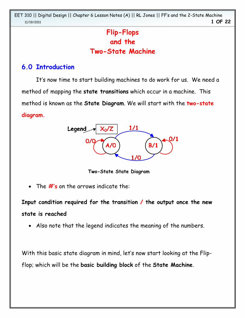
6.0 Introduction
It’s now time to start building machines to do work for us. We need a
method of mapping the state transitions which occur in a machine. This
method is known as the State Diagram. We will start with the two-state
diagram.
The #’s on the arrows indicate the:
Input condition required for the transition / the output once the new
state is reached
Also note that the legend indicates the meaning of the numbers.
With this basic state diagram in mind, let’s now start looking at the Flip-
flop; which will be the basic building block of the State Machine.
Two-State State Diagram

EET 310 || Digital Design || Chapter 6 Lesson Notes (A) || RL Jones || FF’s and the 2-State Machine 11/19/2011 2 OF 22
6.1 The Latch and Flip-Flop in general
Flip-Flops are very important to the construction of counters and state
machines. They generally consist of a clock input, one or two synchronous
control inputs (D, T, or J and K), one or two asynchronous control inputs
(Preset and Clear), and usually two outputs, one the inverse of the other.
The sections to follow will cover the basics of how the Flip-flops are built.
6.1.1 The simple latch
The simplest form of memory device is the latch. The figure below is
an example of a “Permanently Sticking Latch.”
If you power this latch up in a ‘0’ state, the output is ‘0’.
If the input becomes a ‘1’, the output becomes a ‘1’.
If the input goes back to a ‘0’, the output remains at ‘1’.
This is known as the Permanently Sticking Latch.
The Permanently Sticking latch
EET 310 || Digital Design || Chapter 6 Lesson Notes (A) || RL Jones || FF’s and the 2-State Machine 11/19/2011 3 OF 22
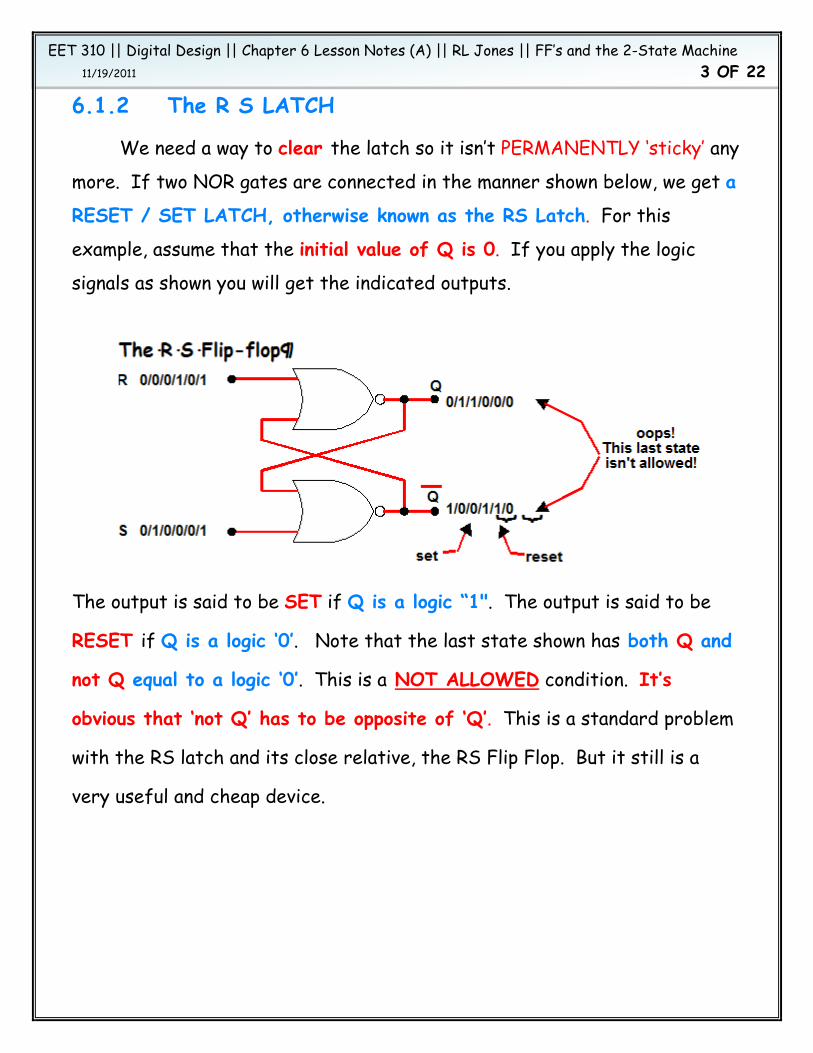
6.1.2 The R S LATCH
We need a way to clear the latch so it isn’t PERMANENTLY ‘sticky’ any
more. If two NOR gates are connected in the manner shown below, we get a
RESET / SET LATCH, otherwise known as the RS Latch. For this
example, assume that the initial value of Q is 0. If you apply the logic
signals as shown you will get the indicated outputs.
The output is said to be SET if Q is a logic “1". The output is said to be
RESET if Q is a logic ‘0’. Note that the last state shown has both Q and
not Q equal to a logic ‘0’. This is a NOT ALLOWED condition. It’s
obvious that ‘not Q’ has to be opposite of ‘Q’. This is a standard problem
with the RS latch and its close relative, the RS Flip Flop. But it still is a
very useful and cheap device.

EET 310 || Digital Design || Chapter 6 Lesson Notes (A) || RL Jones || FF’s and the 2-State Machine 11/19/2011 4 OF 22
6.2 Improving the Latch
A significant problem with latches in general is that the propagation
delays inherent in the latch could be a source of possible error if several of
them were cascaded together. What we need to do is find a way to
synchronize all of the latches so they would all have delays which all start at
the same time.
The best way to accomplish this is to use the “inhibit gate” concept
which you learned about in basic digital. If we use a clock signal as the
switch for the “inhibit gate” we now can block the ‘S’ and ‘R’ signals from
reaching the latch until it is desired to be there (see Figure below). If we
use the same clock signal to all the latches we now have reduced the
possibility of propagation delay problems.
We can also add in an additional input to each NOR gate in order to change
the output states independent of the clock input. Whenever you have
inputs which are independent of the synchronizing effect of a clock input,
those inputs are known as asynchronous inputs. In this case, the inputs are
Preset ‘PRE’ and Clear ‘CLR’ which either SET the Q output to 1 or CLEAR it
to a 0 respectively.
EET 310 || Digital Design || Chapter 6 Lesson Notes (A) || RL Jones || FF’s and the 2-State Machine 11/19/2011 5 OF 22
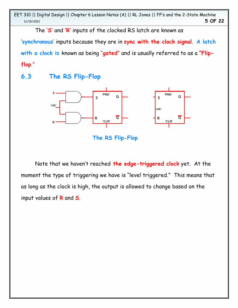
The ‘S’ and ‘R’ inputs of the clocked RS latch are known as
‘synchronous’ inputs because they are in sync with the clock signal. A latch
with a clock is known as being “gated” and is usually referred to as a “Flip-
flop.”
6.3 The RS Flip-Flop
Note that we haven’t reached the edge-triggered clock yet. At the
moment the type of triggering we have is “level triggered.” This means that
as long as the clock is high, the output is allowed to change based on the
input values of R and S.
The RS Flip-Flop

EET 310 || Digital Design || Chapter 6 Lesson Notes (A) || RL Jones || FF’s and the 2-State Machine 11/19/2011 6 OF 22
The timing diagram in Figure
6 demonstrates that
whenever the clock is high, an
action window opens up in
which commands on the R
and/or S inputs are allowed to affect the output. (Note that the timing
diagram shown doesn’t take into account Set-up times, Hold times, or
Propagation Delay times). The transition table which governs how the
output will respond to the RS commands is given in Section 6.3.2.
6.3.1 Present and Next State Definitions:
Before we start looking at transition tables, we need to define two
terms, QP and QN.
QP = Q present = Present state:
The state of the output before the clock signal.
QN = Q next = Next state:
The state the output will attain based on the flip-flop synchronous
inputs after the clock signal occurs. It is a prediction of what will
happen in the FUTURE!
These two definitions are extremely important to your future
understanding of state-machines and how flip-flops act!
Clock
R
S
Q
Figure 66
EET 310 || Digital Design || Chapter 6 Lesson Notes (A) || RL Jones || FF’s and the 2-State Machine 11/19/2011 7 OF 22
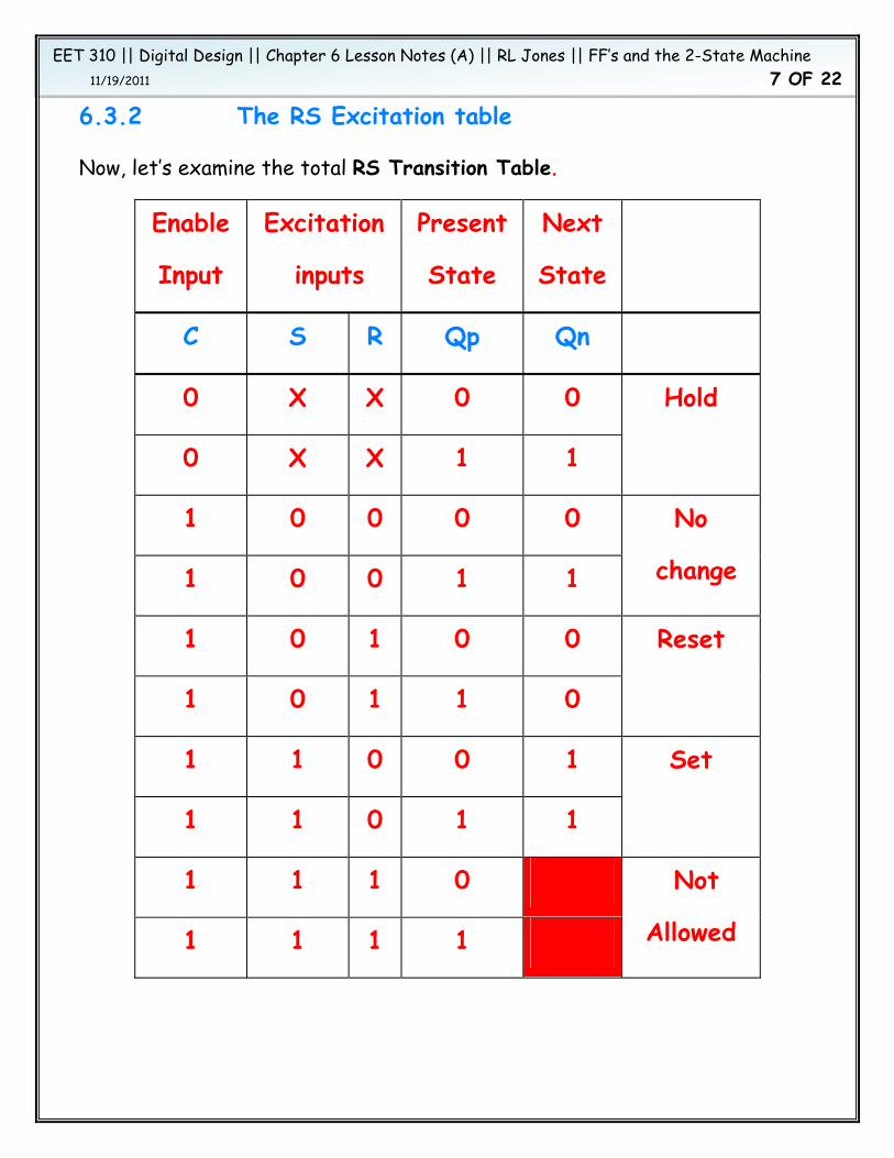
6.3.2 The RS Excitation table
Now, let’s examine the total RS Transition Table.
Enable
Input
Excitation
inputs
Present
State
Next
State
C S R Qp Qn
0 X X 0 0 Hold
0 X X 1 1
1 0 0 0 0 No
change 1 0 0 1 1
1 0 1 0 0 Reset
1 0 1 1 0
1 1 0 0 1 Set
1 1 0 1 1
1 1 1 0 Not
Allowed 1 1 1 1
EET 310 || Digital Design || Chapter 6 Lesson Notes (A) || RL Jones || FF’s and the 2-State Machine 11/19/2011 8 OF 22
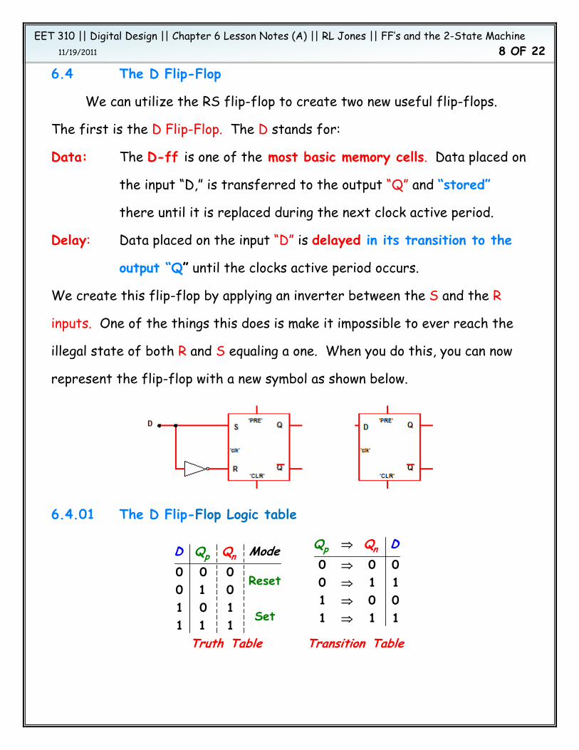
6.4 The D Flip-Flop
We can utilize the RS flip-flop to create two new useful flip-flops.
The first is the D Flip-Flop. The D stands for:
Data: The D-ff is one of the most basic memory cells. Data placed on
the input “D,” is transferred to the output “Q” and “stored”
there until it is replaced during the next clock active period.
Delay: Data placed on the input “D” is delayed in its transition to the
output “Q” until the clocks active period occurs.
We create this flip-flop by applying an inverter between the S and the R
inputs. One of the things this does is make it impossible to ever reach the
illegal state of both R and S equaling a one. When you do this, you can now
represent the flip-flop with a new symbol as shown below.
6.4.01 The D Flip-Flop Logic table
0 0 00 0 00 1 10 1 01 0 0
Reset
S
et1 0 1
1 1 11 1 1
p nnp M QQ
Truth Table Transi
o
tion T
D
ab
eD d
l
Q
e
Q

EET 310 || Digital Design || Chapter 6 Lesson Notes (A) || RL Jones || FF’s and the 2-State Machine 11/19/2011 9 OF 22
6.4.02 Setup and Hold Times
The D flip-flop acts as shown in the timing diagrams below. Note the
concept of Setup and Hold times that you should have learned about in
basic digital and which were discussed earlier in this text. While all FF’s are
affected by the times, for this course, as a general rule, we will assume that
both of these times are equal to 0.

EET 310 || Digital Design || Chapter 6 Lesson Notes (A) || RL Jones || FF’s and the 2-State Machine 11/19/2011 10 OF 22
With the circuit setup the way we have it now, we may see some
unstable behavior. One way to fix this behavior is to create a system known
as Master/Slave circuits. This system creates a buffering arrangement
which eliminates the unstable behavior. However, the master/slave circuit
is going out of style and is for the most part is being replaced by the
edge-triggered f/f.
6.4.1 The Edge-Triggered Clock
In this system we use the circuit below to cause the device to trigger
on the leading or trailing edge of the clock.
This sensitivity to only the edge of the clock pulse eliminates the unstable
transients by drastically reducing the period during which the excitation
signals are applied to the internal latches.
EET 310 || Digital Design || Chapter 6 Lesson Notes (A) || RL Jones || FF’s and the 2-State Machine 11/19/2011 11 OF 22
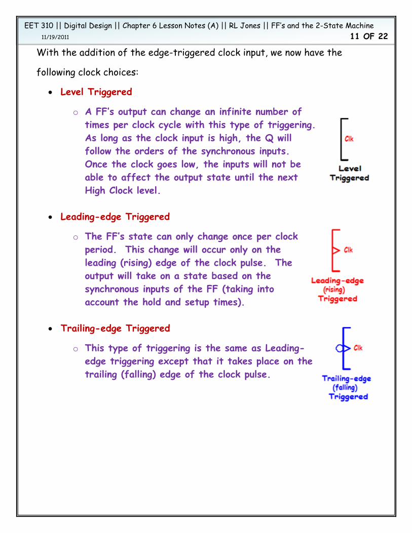
With the addition of the edge-triggered clock input, we now have the
following clock choices:
Level Triggered
o A FF’s output can change an infinite number of times per clock cycle with this type of triggering. As long as the clock input is high, the Q will follow the orders of the synchronous inputs. Once the clock goes low, the inputs will not be able to affect the output state until the next High Clock level.
Leading-edge Triggered
o The FF’s state can only change once per clock period. This change will occur only on the leading (rising) edge of the clock pulse. The output will take on a state based on the synchronous inputs of the FF (taking into account the hold and setup times).
Trailing-edge Triggered
o This type of triggering is the same as Leading-edge triggering except that it takes place on the trailing (falling) edge of the clock pulse.

EET 310 || Digital Design || Chapter 6 Lesson Notes (A) || RL Jones || FF’s and the 2-State Machine 11/19/2011 12 OF 22
6.5 The T-FF
The tables for the T-FF are:
0 0 00 0 00 1 1Hold
Toggle
0 1 11 0 11 0 11 1 01 1 0
pp
nn Mode QQ
Truth Table Transitio
TT
T ble
Q
n a
Q
6.5 The JK FF
By adding a couple of additional gates to the D-FF, we can create a new
circuit building block, the JK-FF.

EET 310 || Digital Design || Chapter 6 Lesson Notes (A) || RL Jones || FF’s and the 2-State Machine 11/19/2011 13 OF 22
J K Qp Qn 0 0 0 0
Hold 0 0 1 1 0 1 0 0
Reset 0 1 1 0 1 0 0 1
Set 1 0 1 1 1 1 0 1
Toggle 1 1 1 0
With this change, we no longer have to worry about the 1/1 input
condition of the RS FF. As a matter of fact, we can pretty well leave the
RS-FF in the ‘dust-bin of technology’ (my opinion).

EET 310 || Digital Design || Chapter 6 Lesson Notes (A) || RL Jones || FF’s and the 2-State Machine 11/19/2011 14 OF 22
6.5.1 The JK used as a T-FF
The table to the right is an excerpt of
the JK truth table above. Note that the 1st
two rows have both JK = 00. In this HOLD
condition, any change in the output is
impossible.
The last two rows in the truth table have both JK = 11 in common. In
this condition, if the Present State is 0, the Next State will be 1, while if
the Present State is a 1, the Next State will be a 0. This is called a
“TOGGLE” condition. Since the JK inputs are the
same in each pair, we can short them together to
create a single input called “T.” This now forms a
“T-ff.”
The T-FF Truth table now looks like the
one to the left.
J K Qp Qn
0 0 0 0 }
Hold 0 0 1 1
1 1 0 1 }
Toggle 1 1 1 0
T Qp Qn
0 0 0 Hold Mode
0 1 1
1 0 1 Toggle Mode 1 1 0

EET 310 || Digital Design || Chapter 6 Lesson Notes (A) || RL Jones || FF’s and the 2-State Machine 11/19/2011 15 OF 22
We can reorganize this table to form
what is known as a “T” Transition Table
as shown here:
6.5.2 The JK used as a D-ff
Again we have an excerpt from the JK truth
table. This time note that in rows three and
four, J and k are opposite values, JK = 01.
This condition mimics the D-ff Reset
condition that we discussed earlier. In this
condition, no matter what the present state
is, the next state will be a 0.
Now note that in rows five and six, J and K are again opposite values,
but this time, JK = 10. This is the “Set” condition which again means that
no matter what the present state is, the next state will be a 1.
In order to implement this flip flop using a JK flip-
flop, an inverter must be placed between the J and
the K inputs to make it impossible for the J and the
K inputs to ever be the same value.
Qp ➔ Qn T
0 ➔ 0 0
0 ➔ 1 1
1 ➔ 0 1
1 ➔ 1 0
J K Qp Qn
0 1 0 0 }
Reset 0 1 1 0
1 0 0 1 }
Set 1 0 1 1

EET 310 || Digital Design || Chapter 6 Lesson Notes (A) || RL Jones || FF’s and the 2-State Machine 11/19/2011 16 OF 22
The truth table for the D-ff now looks like this:
D Qp Qn
0 0 0
0 1 0
1 0 1
1 1 1
We can reorganize this table to form what is known as a “D” transition table
as shown to the right. Note that the D flip flop column is exactly the same
as the Next State column (Qn). In the D flip-flop, D and Next state will
“ALWAYS BE THE SAME!”
Qp ➔ Qn D
0 ➔ 0 0
0 ➔ 1 1
1 ➔ 0 0
1 ➔ 1 1
Note that all three flip-flops discussed have trailing edge clocks and
ACTIVE LOW Preset and Clear inputs. This is by no means the rule; it was
just my choice. No matter what you do, when selecting a flip flop, make sure
you know what type of inputs you are getting.

EET 310 || Digital Design || Chapter 6 Lesson Notes (A) || RL Jones || FF’s and the 2-State Machine 11/19/2011 17 OF 22
6.5.2 The JK used as a JK
Since both the T and the D flip flops have transition tables, it follows that
the JK should as well. Let’s take a second look at the JK truth table.
Note that the other tables had four rows while this one has eight rows. So,
in the process of creating the transition table, it would be nice if the
number of rows in the table could be four as well.
To do this we need to remember the “Don’t Care” condition. In this
case, there are parts of the table where either the state of J or of K
doesn’t matter to the transition of the output from Present state to Next
state.
Row J K Qp Qn
1 0 0 0 0 }
Hold 2 0 0 1 1
3 0 1 0 0 }
Reset 4 0 1 1 0
5 1 0 0 1 }
Set 6 1 0 1 1
7 1 1 0 1 }
Toggle 8 1 1 1 0

EET 310 || Digital Design || Chapter 6 Lesson Notes (A) || RL Jones || FF’s and the 2-State Machine 11/19/2011 18 OF 22
The transition from Qp = 0 to Qn = 0 (rows 1 and 3):
Note in the row 1 & 3 table that in both rows, J = 0, while K takes on
both a 0 and a 1. No matter what K is equal to, if J = 0 and the Present
state is 0, the next state will be reset to a 0. In other words, we “Don’t
Care” what state K is in.
p np n
Q QQ Q
0 00 00
RowRow
1KJ
0
J K0
X1 10
003
The transition from Qp = 0 to Qn = 1 (rows 5 and 7):
Note in the row 5 & 7 table that in both rows, J = 1, while K takes on
both a 0 and a 1. No matter what K is equal to, if J = 1 and the Present
state is 0, the next state will be set to a 1. In other words, we “Don’t
Care” what state K is in.
p np n
Q QQ Q
0 10 10
RowRow
5KJ
1
J K0
X1 21
117
EET 310 || Digital Design || Chapter 6 Lesson Notes (A) || RL Jones || FF’s and the 2-State Machine 11/19/2011 19 OF 22
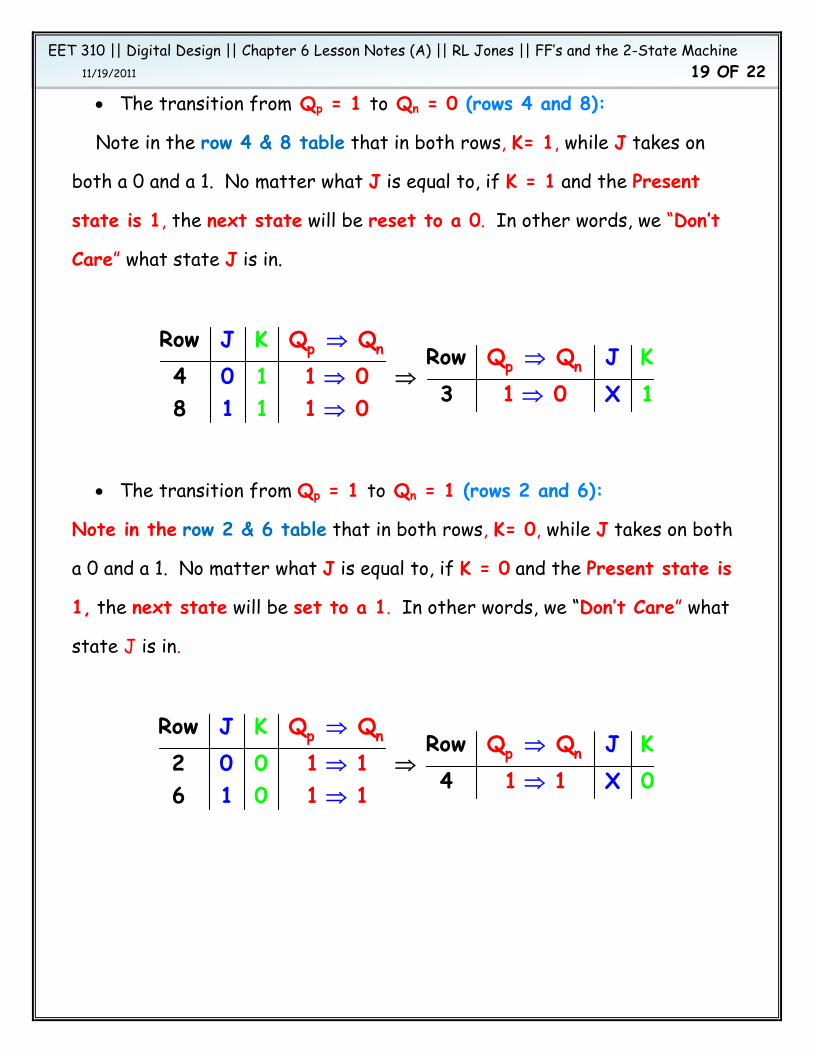
The transition from Qp = 1 to Qn = 0 (rows 4 and 8):
Note in the row 4 & 8 table that in both rows, K= 1, while J takes on
both a 0 and a 1. No matter what J is equal to, if K = 1 and the Present
state is 1, the next state will be reset to a 0. In other words, we “Don’t
Care” what state J is in.
p np n
Q QQ Q
1 01 01
RowRow
4KJ
0
J K1
11 30
X18
The transition from Qp = 1 to Qn = 1 (rows 2 and 6):
Note in the row 2 & 6 table that in both rows, K= 0, while J takes on both
a 0 and a 1. No matter what J is equal to, if K = 0 and the Present state is
1, the next state will be set to a 1. In other words, we “Don’t Care” what
state J is in.
p np n
Q QQ Q
1 11 11
RowRow
2KJ
1
J K0
00 40
X16
EET 310 || Digital Design || Chapter 6 Lesson Notes (A) || RL Jones || FF’s and the 2-State Machine 11/19/2011 20 OF 22
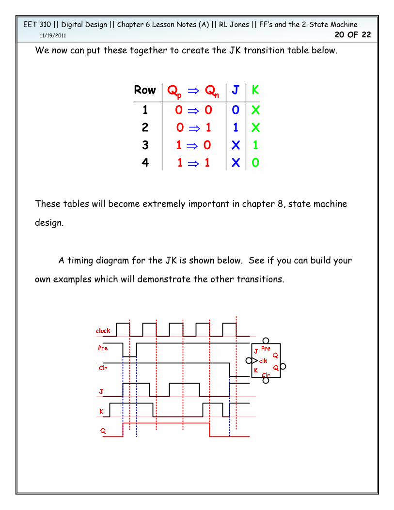
We now can put these together to create the JK transition table below.
p nQ Q0 00
J01
Row123
11 0 X
KXX1
1 X1 04
These tables will become extremely important in chapter 8, state machine
design.
A timing diagram for the JK is shown below. See if you can build your
own examples which will demonstrate the other transitions.

EET 310 || Digital Design || Chapter 6 Lesson Notes (A) || RL Jones || FF’s and the 2-State Machine 11/19/2011 21 OF 22
Let’s take a look at Example 6-1 from the book. The author used a short-hand way of showing the State table and left out the Legend from the state diagram. For these reasons, we will go ahead and work that example here. Prob. Statement: Consider a sequential circuit having one
input (x), two states (y2 and y1), and one output variable (z). (Note: The book got y2 and y1 backwards). Make the indicated state assignments. The initial condition of the machine (yo) is state A.
If the circuit has the following input sequence applied to it: x=0110101100, the following behavior will be observed:
0 1 1 0 1 0 1 1 0 0A D B A D B B A C C C
Trigger 0 1 2 3 4 5 6 7 8 9 10xPSNSz
D B A D B B A C C C0 1 0 0 1 1 0 1 1 1
Next we need to produce the state table from this information. I will start with the larger version, then go to a smaller version (for your information). The two rows in red (x=0, D goes to A and x=1, C goes to D) are unspecified, or “illegal” states and are assigned by the designer (me).
State Assignment
2 1
A 00B 01
State y y
C 10D 11
2 1 2 1x y y z
0 1 D 1
0 0 A 0 1 D 1 00 0 B 1 0 B 1 10 1 C 0 1 C 0 1
1 0 A 0 1 C 0 11 0 B 1 0 A 0
0 A 0 0
1 1 C 0 10
1 1 D 1D 1
1 10
0 B
Y Y

EET 310 || Digital Design || Chapter 6 Lesson Notes (A) || RL Jones || FF’s and the 2-State Machine 11/19/2011 22 OF 22
The larger table can be converted into a short-hand table:
2 1
0 A 0 D / 0 C / 10 B 1 B
PS NS
/ 1 A / 01 C 0 C / 1 D / 01 D 1 A / 0
Xy y / z
X
B 1
0 1
/
/ z
2 1 2 1Y Y Y Y
Now we can create the state diagram:
2 1 2 1x y y z
0 1 D 1
0 0 A 0 1 D 1 00 0 B 1 0 B 1 10 1 C 0 1 C 0 1
1 0 A 0 1 C 0 11 0 B 1 0 A 0
0 A 0 0
1 1 C 0 10
1 1 D 1D 1
1 10
0 B
Y Y