Note Set #17.5• MATLAB Examples• Reading Assignment: MATLAB Tutorial on Course Webpage

EEO 401 Digital Signal Processing

Prof. Mark Fowler

1/24

Type commands here on the Command Line in the Command Window

Workspace shows variables you’ve

created

Command History gives access to your previous

commands

Current folder

name here

Folder Navigation

Contents of Current Folder

Click here to go back to default view

Click here for Help

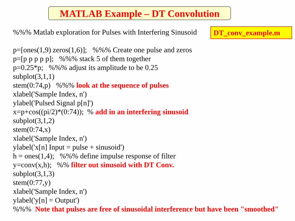
MATLAB Example – DT Convolution

%%% Matlab exploration for Pulses with Interfering Sinusoid

p=[ones(1,9) zeros(1,6)]; %%% Create one pulse and zerosp=[p p p p p]; %%% stack 5 of them togetherp=0.25*p; %%% adjust its amplitude to be 0.25subplot(3,1,1)stem(0:74,p) %%% look at the sequence of pulsesxlabel('Sample Index, n')ylabel('Pulsed Signal p[n]')x=p+cos((pi/2)*(0:74)); % add in an interfering sinusoidsubplot(3,1,2)stem(0:74,x)xlabel('Sample Index, n')ylabel('x[n] Input = pulse + sinusoid')h = ones(1,4); %%% define impulse response of filtery=conv(x,h); %% filter out sinusoid with DT Conv.subplot(3,1,3)stem(0:77,y)xlabel('Sample Index, n')ylabel('y[n] = Output')%%% Note that pulses are free of sinusoidal interference but have been "smoothed"

DT_conv_example.m

-1 -0.8 -0.6 -0.4 -0.2 0 0.2 0.4 0.6 0.8 10

1

2

3

4

Ω/π (normalized radians/sample)

|H( Ω

)|

-1 -0.8 -0.6 -0.4 -0.2 0 0.2 0.4 0.6 0.8 1-4

-2

0

2

4

Ω/π (normalized radians/sample)

<H( Ω

) (r

ad)

-1 -0.5 0 0.5 1

-1

-0.8

-0.6

-0.4

-0.2

0

0.2

0.4

0.6

0.8

1

3

Real Part

Imag

inar

y P

artx=p+cos((pi/2)*(0:74));

h = ones(1,4);

w=-pi:0.001:pi;H=freqz(h,1,w);zplane(h,1)

When computing the DFT (using fft) you get N numbers that tell the values the DFT coefficients have. But you need to know what frequencies they are at…

We’ll assume that you are using fftshift, which moves the DFT coefficients around so they lie in the frequency range -π to π

To plot versus f in Hz:• For N DFT points… the frequency spacing between them is • With fftshift, the frequencies start at –Fs/2• Thus the command that makes these frequency points is

f = ( (-N/2):( (N/2) -1 ) )*Fs/N

sF N

To plot versus Ω in rad/sample:• For N DFT points… the frequency spacing between them is • With fftshift, the frequencies start at -π• Thus the command that makes these frequency points is

omega = ( (-N/2):( (N/2) -1 ) )*2*pi/N

2 Nπ

Example for our N=8 case: omega = (-4:3)*2*pi/8

gives the vector [-pi -3pi/4 -pi/2 –pi/4 0 pi/4 pi/2 3pi/4]

8 pointsStarts at piStops “just shy of pi”

8/20

MATLAB Trick: Create Frequency Vector for DFT Plotting

Imagine you are in a recording studio and recorded what you feel is a “perfect take” of a guitar solo

But some nearby electronic device caused sinusoidal EM radiation that was picked up somewhere in the audio electronics and was recorded on top of the guitar solo.

Rather than try to recreate this “perfect take” you decide that maybe you can design a DT filter to remove it.

To explore this we’ll SIMULATE it in MATLAB!!

Assume the sinusoid has frequency of 10 kHz

MATLAB Demo: FIR Filter Design & Application

FIR_Filter_Demo.m

[x,Fs]=wavread('guitar1.wav');x=x.'; % convert into row vectoromega=2*pi*(10000/Fs); N=length(x);n=0:(N-1);x_10=x+cos(omega*n);t=(0:49999)*(1/Fs);plot(t,x_10(1:50000),'r',t,x(1:50000))

X=fftshift(fft(x(20000+(1:16384)),65536));X_10=fftshift(fft(x_10(20000+(1:16384)),65536));f=(-32768:32767)*Fs/65536;subplot(2,1,1); plot(f/1e3,20*log10(abs(X_10)));subplot(2,1,2); plot(f/1e3,20*log10(abs(X)));

Now… look at DFT to see impact in frequency domain:

Use the “firpmord” and “firpm” commands to design lowpass filter to get:

• 60 dB of attenuation in the stopband for the undesired signal

• 1 dB of passband ripple

• passband edge at 7kHz

• stopband edge at 9 kHz.

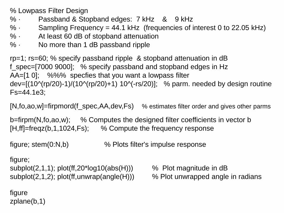
% Lowpass Filter Design% · Passband & Stopband edges: 7 kHz & 9 kHz% · Sampling Frequency = 44.1 kHz (frequencies of interest 0 to 22.05 kHz)% · At least 60 dB of stopband attenuation% · No more than 1 dB passband ripple

rp=1; rs=60; % specify passband ripple & stopband attenuation in dBf_spec=[7000 9000]; % specify passband and stopband edges in HzAA=[1 0]; %%% specfies that you want a lowpass filterdev=[(10^(rp/20)-1)/(10^(rp/20)+1) 10^(-rs/20)]; % parm. needed by design routineFs=44.1e3;

[N,fo,ao,w]=firpmord(f_spec,AA,dev,Fs) % estimates filter order and gives other parms

b=firpm(N,fo,ao,w); % Computes the designed filter coefficients in vector b[H,ff]=freqz(b,1,1024,Fs); % Compute the frequency response

figure; stem(0:N,b) % Plots filter's impulse response

figure; subplot(2,1,1); plot(ff,20*log10(abs(H))) % Plot magnitude in dBsubplot(2,1,2); plot(ff,unwrap(angle(H))) % Plot unwrapped angle in radians

figurezplane(b,1)

-1 -0.5 0 0.5 1

-1

-0.5

0

0.5

1

43

Real Part

Imag

inar

y Pa

rt

Remove Interference with Filter 1. Use the designed filter to remove the interference

− Filter x_10 using the LPF to get x_10_out

y = filter(b,a,x) filters the data in vector x with the filter described by vectors a and b to create the filtered data y.

The vectors a and b come from the coefficients in the difference equation:

∑∑==

−=−ba N

ii

N

ii inxbinya

00][][ a = [a0 a1 a2 … aNa ]

b = [b0 b1 b2 … bNb ]

For an FIR filter like we have here the difference equation is:

∑=

−=N

ii inxbny

0][][ so the “a vector” is a = [a0 ] = 1

2. Assess the performance of the filter:

− Compare x_10_out, x_10, and x in the frequency domain.

− Compare x_10_out, x_10, and x in the time domain.

− Listen to the filtered guitar signal using MATLAB’s sound command.

Remove Interference w/ Filter

x_10_out=filter(b,1,x_10); %%% filter the signal with the designed filter

X_10_out=fftshift(fft(x_10_out(20000+(1:16384)),65536));

figuresubplot(3,1,1); plot(f/1e3,20*log10(abs(X_10))); title('DFT of Signal w/ Interference')

subplot(3,1,2); plot(f/1e3,20*log10(abs(X_10_out))); title('DFT of Filtered Signal')

subplot(3,1,3); plot(f/1e3,20*log10(abs(X))); title('DFT of Original Signal')

figuresubplot(3,1,1); plot(t,x_10(1:50000),'r'); title('Signal w/ Interference')

subplot(3,1,2); plot(t,x(1:50000),'b',t,x_10_out(1:50000),'m--'); title('Filtered Signal and Original')

subplot(3,1,3) %%%%% Make a plot that accounts for the delay in the filtered signal%%% For an odd filter order N the delay is (N-1)/2plot(t,x(1:50000),'b',t,x_10_out(22+(1:50000)),'m--')

Using the same guitar signal…

Suppose we want to design a DT filter that will emphasize the “middle” audio frequencies in that recording… to get a “different sounding” recording…

We’ll explore this in MATLAB!!

MATLAB Demo: IIR Filter “Design” & Application

IIR_Filter_Demo.m

X=fftshift(fft(x(20000+(1:16384)),65536));f=(-32768:32767)*Fs/65536;plot(f/1e3,20*log10(abs(X)));

Now… look at DFT of guitar signal to see it in frequency domain:

DFT of Guitar Signal

Suppose we decide that 1 kHz is the narrow region we want to emphasize

So… what might our frequency response look like?DFT of Guitar Signal

-1 -0.5 0 0.5 1

-1

-0.8

-0.6

-0.4

-0.2

0

0.2

0.4

0.6

0.8

1

Real Part

Imag

inar

y P

art

So… what might our pole-zero plot look like?

-1 -0.5 0 0.5 1

-1

-0.8

-0.6

-0.4

-0.2

0

0.2

0.4

0.6

0.8

1

Real Part

Imag

inar

y P

art

Maybe this would be good….

Ω Needs to correspond to 1000 Hz

0.14 0.14

( 1)( 1)( )( 0.99 )( 0.99 )j j

z zH zz e z e−

+ −=

− −

2 21000 1000 0.1444100sF

π πΩ = = ≈

2

2

11.9606 0.9801

zz z

−=

− +

2

1 2

1( )1 1.9606 0.9801

zH zz z

−

− −

−=

− +

Now… how do we check the actual frequency response?

Omega = -pi:0.001:pi;H=freqz([1 0 -1],[1 -1.9606 0.9801],Omega);f = Omega*Fs/(2*pi);plot(f/1000,20*log10(abs(H)))

2

1 2

1( )1 1.9606 0.9801

zH zz z

−

− −

−=

− +

2

2

1( )1 1.9606 0.9801

j

j jeH

e e

− Ω

− Ω − Ω

−Ω =

− +

-20 -15 -10 -5 0 5 10 15 20

-20

0

20

40

f (kHz)

|H(f

)| (d

B)

Pretty High!!! Gain of 40 dB is 10,000 times more power!!!

Now… apply filter and listen.

H=freqz(0.05*[1 0 -1],[1 -1.9606 0.9801],Omega);plot(f/1000,20*log10(abs(H)))

So… put an overall “gain” term out front…

-20 -15 -10 -5 0 5 10 15 20

-40

-20

0

20

f (kHz)

|H(f

)| (d

B)

g_f=filter(0.05*[1 0 -1],[ 1.0000 -1.9606 0.9801],x);sound(g_f,Fs)

We hear some change… can we take this a bit farther?

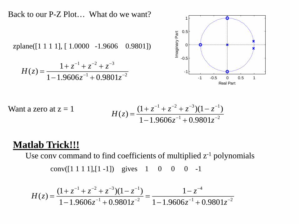
Back to our P-Z Plot… What do we want?

zplane([1 1 1 1], [ 1.0000 -1.9606 0.9801])

1 2 3

1 2

1( )1 1.9606 0.9801

z z zH zz z

− − −

− −

+ + +=

− +

Want a zero at z = 1 1 2 3 1

1 2

(1 )(1 )( )1 1.9606 0.9801

z z z zH zz z

− − − −

− −

+ + + −=

− +

Matlab Trick!!!Use conv command to find coefficients of multiplied z-1 polynomials

conv([1 1 1 1],[1 -1]) gives 1 0 0 0 -1

-1 -0.5 0 0.5 1-1

-0.5

0

0.5

1

Real Part

Imag

inar

y P

art

1 2 3 1 4

1 2 1 2

(1 )(1 ) 1( )1 1.9606 0.9801 1 1.9606 0.9801

z z z z zH zz z z z

− − − − −

− − − −

+ + + − −= =

− + − +

4

1 2

1( )1 1.9606 0.9801

zH zz z

−

− −

−=

− +

zplane([1 0 0 0 -1 ], [ 1.0000 -1.9606 0.9801])

-1 -0.5 0 0.5 1-1

-0.5

0

0.5

1

2

Real Part

Imag

inar

y P

art

Now… an interesting thing comes from exploration of this form with EVEN integer p

1 2

1( )1 1.9606 0.9801

pzH zz z

−

− −

−=

− +

zplane([1 0 0 0 0 0 -1 ], [ 1.0000 -1.9606 0.9801])

zplane([1 zeros(1,5) -1 ], [ 1.0000 -1.9606 0.9801])

-1 -0.5 0 0.5 1-1

-0.5

0

0.5

1

4

Real Part

Imag

inar

y P

art

One last thing… We’d like another zero at z = 1 to push the FR down at low frequencies.

>> conv([1 zeros(1,5) -1],[1 -1])

ans =

1 -1 0 0 0 0 -1 1

zplane([1 -1 zeros(1,4) -1 1 ], [ 1.0000 -1.9606 0.9801])

-1 -0.5 0 0.5 1-1

-0.5

0

0.5

1

25

Real Part

Imag

inar

y P

art

Taking this to an the extreme….

zplane([1 -1 zeros(1,22) -1 1 ], [ 1.0000 -1.9606 0.9801])

-1 -0.5 0 0.5 1-1

-0.5

0

0.5

1

223

Real Part

Imag

inar

y P

art

H = freqz(0.05*[1 -1 zeros(1,22) -1 1 ], [ 1.0000 -1.9606 0.9801],Omega);plot(f/1000,20*log10(abs(H)))

-20 -15 -10 -5 0 5 10 15 20-50

-40

-30

-20

-10

0

10

20

f (kHz)

|H(f

)| (d

B)

g_f=filter(0.05*[1 -1 zeros(1,22) -1 1 ],[ 1.0000 -1.9606 0.9801],x);sound(g_f,Fs)

DFT of Guitar Signal

-20 -15 -10 -5 0 5 10 15 20

-60

-40

-20

0

20

40

60

80

f (kHz)

|DF

T| (

dB)

DFT of Filtered Guitar Signal