Abstract— Fatigue is the most vital factor of road fatalities and one manifestation of fatigue during driving is drowsiness. In this

paper, we propose using deep Q-learning to analyze an electroencephalogram (EEG) dataset captured during a simulated endurance

driving test. By measuring the correlation between drowsiness and driving performance, this experiment represents an important

brain-computer interface (BCI) paradigm especially from an application perspective. We adapt the terminologies in the driving test

to fit the reinforcement learning framework, thus formulate the drowsiness estimation problem as an optimization of a Q-learning

task. By referring to the latest deep Q-Learning technologies and attending to the characteristics of EEG data, we tailor a deep Q-

network for action proposition that can indirectly estimate drowsiness. Our results show that the trained model can trace the

variations of mind state in a satisfactory way against the testing EEG data, which demonstrates the feasibility and practicability of

this new computation paradigm. We also show that our method outperforms the supervised learning counterpart and is superior for

real applications. To the best of our knowledge, we are the first to introduce the deep reinforcement learning method to this BCI

scenario, and our method can be potentially generalized to other BCI cases.

Index Terms— Brain-Computer Interface (BCI), Deep Q-Learning, Driving Safety, Electroencephalogram (EEG), Reinforcement

Learning

I. INTRODUCTION

Fatigue is regarded as the most severe factor causing road fatalities [1]. To understand the correlation between fatigue and

driving performance, both from theory to practice, is of persistent interest for researchers. There have already been many

attempts and much effort spent in understanding the impact of fatigue - like drowsiness on drivers’ response [2], among which

research via EEG is one promising way [5], especially embracing the likelihood that dry sensors are maturing to the stage of

high-quality EEG signal acquisition. Via potential portable EEG device by monitoring brain state, brain can directly

communicate with the driving environment in a spontaneous and passive way to ensure the driving safety.

However, due to the characteristics of brain structures, direct measurement of the mind state, such as drowsy or alert, is

extremely difficult. Hence, the study of driving safety is usually carried out in a lab environment via some approaches

ingeniously designed to indirectly measure the mind state [5]. Based on measured performance indicators such as the response

time (RT) [8], some models have been set up to analyze the signals and deployed for application at a later stage.

Although many conclusions have been reached using traditional machine learning methods especially from the supervised

learning perspective, several drawbacks are still present that unavoidably hinder not only the theoretical analysis but also the

real applications in this field. The first problem is the efficiency of data utilization. Because most supervised learning models,

including deep neural networks (DNN), require the regularised input data to be paired with ground-truth labels for training

purpose, some EEG segmentations are unavoidably discarded if there is no corresponding label information. Second, some

models that require measured information such as RT for performance tuning only work in an offline manner and are unsuitable

or impossible for online application especially from an engineering perspective [5].

In this paper, we introduce deep reinforcement learning, specifically deep Q-learning for analyzing EEG data captured in a

driving safety research experiment [9][10]. One of the eminent characteristics of reinforcement learning is the future reward,

in this paper which is represented by a function of the measured RT in some latency, can be used to assess the current action

to take, given the current EEG data segment which viewed as current state. Another aspect is that for reinforcement learning,

although the training phase requires the costly label information (RT) being obtained for reward calculation, for the testing

stage, an optimal policy is always assumed and exploited for action selection, which means that no further deliberate articulated

measured information is needed. These facts suggest a promising potential for analyzing the EEG signals of similar BCI

scenarios for real applications. To the best of our knowledge, we are the first to assess driving safety via EEG using a

reinforcement learning method.

The rest of this paper is structured as follows. In section II, we describe the problem and the simulated experiment in detail

EEG-based Drowsiness Estimation for Driving

Safety using Deep Q-Learning

Yurui Ming, Dongrui Wu, Yu-Kai Wang, Yuhui Shi, Chin-Teng Lin

to formulate the corresponding reinforcement learning model, followed by section III where the deep Q-network is tailored for

analyzing EEG data captured from the simulated driving safety test. In section IV, by comparing the performance of our method

with that of the corresponding supervised learning model, the practicability of our proposed approach is shown by statistics.

Section V discusses the interesting discovery of using this method from a neurophysiological perspective.

II. PROBLEM DESCRIPTION

A. Driving Safety Research

The investigation of the causality between fatigue and driving performance needs the driver’s implicit mind states and

corresponding reactions. It is more practical to carry out the research in the lab first to simulate the problem, exploring potential

solutions, and assessing the proposed method, etc., for later generalization to real applications. Thus, a simulated environment

is built to mimic the endurance driving scenario to conduct the research.

The experiment is designed as recruited drivers performing an endurance driving along the simulated highway lasting 90

minutes in general, during which the subjects’ physiological state is postulated to be hardly maintained at the same condition.

The experiment was approved by the Institutional Review Board of the Taipei Veterans General Hospital (PN: 101W963,

VGHIRB No.: 2012-08-019BCY), and the voluntary, fully informed consent of the subjects participated in this research was

obtained as required the by accompanying regulations handled for ethical committee review (IRB -TPEVGH SOP 05). Fig. 1

(A) illustrates the driving scenario on a four-lane highway. The horizon for the driver is projected on a large chained screen.

To simulate different driving conditions on the road, a real car is converted and installed on a maneuverable platform with six-

degree freedom to guarantee sufficient flexibility as shown in Fig. 1 (B).

The procedures of the experiment are as follows: the driver operates the car cruising on one lane of the highway. Random

turbulence is deliberately introduced to the car to cause it to deviate from the original cruising lane (event onset). The driver is

instructed on observation to quickly turn the steering wheel (response onset) for compensation to move the car back to the

original lane. Once the car returns to its original cruising state (response offset), the trial is complete. Notably, fatigue can be

attributed to many factors. In this work, our consideration is mainly from drowsiness perspective. To correlate drowsiness with

driving performance, the driver only needs to operate the steering wheel and is freed from brake and petrol panels controlling.

Because fatigue cannot be directly measured, an indirect indicator, aka RT is introduced for this purpose. In detail, the

duration between the event onset to the response onset is termed RT. It measures how quickly the subject reacts to a stimulus.

The period before event onset is called baseline region, the duration of which depends on the setup of trial interval (minimum

5 seconds), and EEG data from this region are nominated for brain dynamic analysis and machine learning application. We

Fig. 1 Simulated driving setup: (A) the mimicking highway scenario; (B) the maneuvering platform with installed converted car.

Fig. 2 Illustration of the experimental scenario. A trial launches from the event onset and extends to the response offset. A session is constituted by repetitive trials.

illustrate the corresponding terminologies which are key to understanding the experiment in Fig. 2. The specifications of the

setup, procedures of the experiment and EEG data acquisition can also be found in [8].

Usually, the number of times for subjects participating in the experiment is not mandatory in order to encourage voluntary

dedication although all subjects are paid. For a certain subject who participated in the experiment, the EEG data captured during

the whole process are called session data. The number of session data for each subject depends on the subject’s participations.

Each session data contains numerous trial data. The interval between consecutive trials is usually randomly 5 to 10 seconds.

The number of trial data in different sessions is highly depending the situation when subjects participated in the experiment, so

it varies as well.

It is emphasized that although there lacks an explicit formula linking RT with the mind state, it is postulated that they are

positively correlated. The correlation can be estimated from the corresponding EEG data captured during the experiment. RT

is sufficient from the application perspective, because by setting a reasonable RT threshold, any RT value above it indicates a

poor control of the car, and a warning should be raised to prevent potential accidents be led.

B. Reinforcement Learning Proposition

Reinforcement learning is inspired by human’s learning process, which is to interact with the environment ℇ by balancing

between the exploration and exploitation of the action 𝑎 at each step for a maximum return 𝐺 in the long run. It requires such

a sequential decision-making process in accordance with the Markov decision process (MDP) for mathematical rigour, which

backs the convergence of the usual iterative optimization process for different reinforcement learning methods [9]. To evaluate

different policies, the state function 𝑉 and value function 𝑄 are defined such that they obey the renowned Bellman equations.

The key terminologies in reinforcement learning are the state 𝑠𝑡, action 𝑎𝑡, reward 𝑟𝑡 and policy 𝜋(∙ |𝑠), etc. For Q-learning, it

is specifically governed by the optimization of (1) in the following:

𝐿𝑡(𝜃𝑡) = 𝔼𝑠,𝑎~𝜌(∙) [(𝑦𝑡 − 𝑄(𝑠, 𝑎; 𝜃𝑡))2

] ()

𝑦𝑡 = 𝔼𝑠′~ℇ [𝑟 + 𝛾 max𝑎′

𝑄(𝑠′, 𝑎′; 𝜃𝑡−1)] ()

where 𝑄 is the value function parameterised by 𝜃. 𝜌(∙) indicates the trajectory distribution, and ℇ indicates the state distribution

in a certain environment [10].

To adjust the driving safety problem resulting in a solution from reinforcement learning algorithms, a retrospect of supervised

learning is presented to highlight the challenges. For supervised learning, the EEG data in the baseline region are extracted and

coupled with the measured RT for training and testing. Exemplified by the work in [5][8], in Fig. 3, only EEG signals covered

by the blue masks are utilized during the analyzing procedures because it is ideal to extract brain dynamic there [6]. Most EEG

data covered by green masks are discarded due to the lack of label or RT information, which means insufficient data utilisation.

A consequent problem is, when deploying the trained supervised learning model for application, the captured EEG data are

continuously input for inference, without distinguishing where the EEG data reside. Such a wider generalisation scope probably

Fig. 3 Data utilisation paradigm of supervised learning. Only EEG data under the blue mask are made use of during training and validation.

Fig. 4 Reinforcement learning paradigm for RT estimation (A) training stage; (B) test stage.

incurs poor performance due to the discrepancy in the distributions among EEG data for training and for application

respectively.

The paradigm of reinforcement learning requires abstraction and instantiation of the agent, environment, state, action and

reward to target a specific problem, which is assumed to comply with MDP. The critic for driving safety is the good estimation

of RT, based on which subsequent actions can be taken. The criterion for preference of estimated RT is that by comparing with

the actual measured RT, the smaller difference the better. Therefore, we need a mechanism to maintain the estimated RT in

order to compare with the measured RT when appropriate (i.e., where there exists measured RT for the current state). To

summarise, the environment can be designed as comprising the captured EEG data and an internal RT tracer. The actions are

issued by the agent to manipulate the tracer to estimate RT. This strategy leads to the design of a reinforcement learning

architecture in Fig. 4.

An instantiation of the reinforcement learning process based on the above depiction is illustrated in Fig. 5. The components

of reinforcement learning are dissected into a concrete representation in the context of session data captured in one experiment.

As shown in Fig. 5, the state 𝑠𝑡 is one piece of the continuously segmented session data, and the action 𝑎𝑡 indicates how to

operate the internal tracer. To fabricate a reward at every time step, the following strategy is taken: if the duration of state 𝑠𝑡

covers a measured RT, 𝑟𝑡 is equal to the negative of the absolute difference between the measured RT and traced RT; otherwise,

the reward 𝑟𝑡 is equal to 0. Note that we take the negative of the absolute value because the optimization targets a maximum

return. Since we focus on Q-learning, the operation to the internal tracer is specially designed to allow only discrete operations.

As shown in Fig. 5, an exemplified action can be chosen to maintain the current traced RT, increase or decrease RT by a certain

unit such as 0.5s.

It is pointed out here although the actions designed above are self-evident from the illustrative perspective, upon

implementation, we use a mechanism called RT proposition. The problem for the action paradigm in Fig. 5 is that the final

estimated RT by tracing is history-dependent. Although it is a more general case than Markov-dependent, it might not be

flexible enough. Actually, it can be postulated that mind state at 𝑡 + 1 only depends on its predecessor at 𝑡. Our empirical

experience can justify this: supposing that we are sleepy at time step 𝑡, we can either feel sleepy or experience sudden alertness

at 𝑡 + 1. Either way, it is not necessary to check the mind state at 𝑡 − 1. This argument leads to the formulation of the up-to-

date traced RT value as follows:

𝑡𝑅𝑇𝑡 = 𝛽 ∙ 𝑡𝑅𝑇𝑡−1 + (1 − 𝛽) ∙ 𝑝𝑅𝑇𝑡 ()

In (3), 𝑡𝑅𝑇 denotes the traced RT; 𝑝𝑅𝑇 denotes the proposed RT at the current time step and can only have discrete values

such as 1.2s, 2.5s, etc., because we consider Q-learning in this paper. 𝛽 is termed the transition weight. Because traced RT is

termed from the illustrative dynamic decision-making perspective, so we use it interchangeably with the term predicted RT.

Notably, compared with supervised learning, which focuses on trial data, reinforcement learning in our design works directly

with session data. To the best of our knowledge, we are the first to introduce reinforcement learning in this field. It is mentioned

that the currently available dataset might pose a challenge for our proposed method, because session data are not abundant due

to the original experiment design. However, as long as the practicability can be demonstrated via the current dataset, it still

indicates a promising beginning for subsequent research. Another point is our design is from prototyping perspective, might

lack the rigor from the field-engineering perspective. For example, the state in our design is the non-overlap EEG segment in

3 seconds. The treatment is just derived from lab convention and might not be the optimal choice.

III. MODEL DESIGN

DeepMind has performed revolutionary work in revising conventional reinforcement learning methods, such as Q-Learning.

They devised deep Q-learning, or deep Q-network (DQN) if the underlying DNN for the Q-function estimation needs to be

Fig. 5 Instantiation of concepts in reinforcement learning in the context of driving safety research.

emphasized [10], which was originally thought to be impractical due to several constraints. They are the first to introduce

several tricks such as temporarily fixed target network parameters during training, experience replay, etc., all of which pave

the way for successfully applying DQN in different fields. They also enhanced DQN by incorporating more techniques from

traditional reinforcement learning and proposed new architectures such as double DQN and duelling DQN [11][12]. Our work

adopts the same tricks during the utilization of DQN and makes some modifications to the experience replay part to achieve

more efficienct computation. As shown in Fig. 6, we add a batch buffer that actually refers to the frames in the replay queue to

avoid unnecessary copying operations. We add a sequence number which in theory can wrap back to 0 for each frame, to adjust

the sample selection.

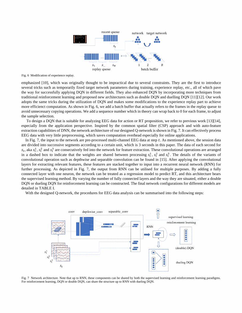
To design a DQN that is suitable for analyzing EEG data for action or RT proposition, we refer to previous work [13][14],

especially from the application perspective. Inspired by the common spatial filter (CSP) approach and with auto-feature

extraction capabilities of DNN, the network architecture of our designed Q-network is shown in Fig. 7. It can effectively process

EEG data with very little preprocessing, which saves computation overhead especially for online applications.

In Fig. 7, the input to the network are pre-processed multi-channel EEG data at step 𝑡. As mentioned above, the session data

are divided into successive segments according to a certain unit, which is 3 seconds in this paper. The data of each second for

𝑠𝑡, aka 𝑠𝑡1, 𝑠𝑡

2 and 𝑠𝑡3 are consecutively fed into the network for feature extraction. These convolutional operations are arranged

in a dashed box to indicate that the weights are shared between processing 𝑠𝑡1 , 𝑠𝑡

2 and 𝑠𝑡3 . The details of the variants of

convolutional operation such as depthwise and separable convolution can be found in [15]. After applying the convolutional

layers for extracting relevant features, these features are stacked together to input into a recurrent neural network (RNN) for

further processing. As depicted in Fig. 7, the output from RNN can be utilised for multiple purposes. By adding a fully

connected layer with one neuron, the network can be treated as a regression model to predict RT, and this architecture bears

the supervised learning method. By varying the number of fully connected layers and the way they are situated, either a double

DQN or dueling DQN for reinforcement learning can be constructed. The final network configurations for different models are

detailed in TABLE I.

With the designed Q-network, the procedures for EEG data analysis can be summarised into the following steps:

Fig. 7 Network architecture. Note that up to RNN, these components can be shared by both the supervised learning and reinforcement learning paradigms. For reinforcement learning, DQN or double DQN, can share the structure up to RNN with dueling DQN.

Fig. 6 Modification of experience replay.

IV. EXPERIMENT

We use the EEG data captured during the simulated driving experiment described above to evaluate our proposed method.

One of the traits for EEG data that might affect the performance is the intra- and cross-subject variance due to numerous factors.

For the experiment, we consider the single-subject case and the multi-subject case separately in the following sections. Because

we are the first to initiate DQN for driving safety research especially from an application perspective, the discrete action space

requires limited RT resolution (due to discrete actions) to approach the measured RT, which in theory is a real number. This

restriction causes difficulty in competing with the previous results achieved by different network structures especially due to

quantization error in this circumstance. In addition, our preprocessing of the EEG data is intended to be lightweight, hence our

main consideration here is not to seek the best network structure to compete with state-of-the-art results, but rather to

demonstrate the feasibility and practicability of this new application oriented computation paradigm for driving safety research

by comparing with supervised learning that has almost the same network structure as shown in Fig. 7.

In general, although EEG signals are complicated due to signal distortion, artefact pending, etc., in this work only limited

preprocessing is applied to the data and measured RT. For EEG signals, a band-pass filter with a range 0.5 to 50 Hz is

introduced, followed by downsampling to 128 Hz from the original sampling rate of 500 Hz. For RT, the values are clipped

into the range 0.5 to 8 second (s), with a moving average within 90 seconds [16]. Finally, the post preprocessed continuous

signals are segmented into consecutive sections with a unit of 3s as shown in Fig. 5.

A. Single-subject Case

Stemming from the fact that the variance of the statistical distributions for EEG data of a single subject is not as severe as

that of multiple subjects, we first consider the single subject case to verify the performance of the proposed model. We choose

subjects of the same gender who had participated in the experiment at least three times. For some sessions, the experiment was

configured to issue warnings upon event onsets, to inspect the influence of explicit arousal on driving performance. We omit

these sessions for consistent experimental scenarios. The subjects who merit the above criteria are S01(4)(1410), S09(3)(704)

and S41(3)(1405). The number in the first parentheses indicates number of session data, aka how many times the subject

participated in the experiment. The number in the second parentheses indicates total trials of all sessions. For each subject, the

data from the first two sessions are for training and the remaining one for testing. One session data of S01 is used for validation

to decide total number of iterations which is applied for model training on all subjects’ data.

We take the dueling DQN architecture due to its performance and train the model for 2000 iterations or episodes with similar

hyperparameters adopted from [10]. The transition weight 𝛽 is set to 0.75. To monitor the convergence of the training process

of our proposed model, two indicators are employed for inspection: the episode return and the average return. The episode

return is the summation of rewards at each step when processing session data. It is a direct measurement of episodic gain but

tends to be noisy. By introducing the average return over episodes, the trend for convergence is relatively more clear; however,

Carry out the experiment to obtain session data

Establish the measured information for reward calculation

Setup parameters like segment length and input the data into the model for training

Test the performance of the model for application

TABLE I NETWORK ARCHITECTURE CONFIGURATION

Model Layer ID Layer Type Filters Size Act. Pad. Comment

CNN

1 Conv2D 32 (1, 64) - Same

2 Depthwise-Conv2D 1 (30, 1) tanh Valid Weight clipping

AvgPool2D - (2, 2) Same

3 Separable-Conv2D 32 (1, 16) tanh Same

AvgPool2D (2, 2) Same

RNN 4 Conv2D 4*3*32 (1, 8) - Same 2D LSTM

Gate-depended activation

Supervised Linear - 512 id L2 Regularization

Linear 1

(Double) DQN Linear - 512 id L2 Regularization

Linear #actions

Dueling DQN

state Linear - 512 id L2 Regularization

Linear 1

state-action Linear - 512 id L2 Regularization

Linear #actions

due to the accumulation effect, there might be a latency of reflection for overfitting. Nevertheless, by combining the two

indicators, the training process can be well monitored. We randomly switch between the data of two sessions during the training

process, and Fig. 8 illustrates the corresponding episode return and average return. The trained model is applied to the test

session data to predict RT in a consecutive way.

As for the benchmarking method, we use the same network structure to construct the regressor and train in supervised

learning, according to Fig. 7 and TABLE I. The preprocessing of EEG data is the same as that for reinforcement learning, then

EEG signals lasting for 3 seconds in the baseline region together with measured RT are grouped to represent the corresponding

trial, as illustrated in Fig. 3. To be consistent with reinforcement learning treatment, trial data constituted the first two sessions

are for training. Trial data of one session of S01 are for validation to decide the total number of iterations for training. The

model is trained with learning rate 0.0001 for 600 iterations for each subject. The trained model is tested on trial data to predict

RT and also made inference on the test session in a consecutive way as the case of reinforcement learning.

To quantitively assess the performance of reinforcement learning and supervised learning in this case, first, only segments

of the test session data where measured RTs exists are considered. We calculate the rooted mean square errors (RMSE) between

the measured RT and the predicted RT for the reinforcement learning model and the supervised learning model respectively.

Second, to investigate the overall consistency between measured RT and predicted RT, we interpolate all segments of test data

Fig. 9 Measured RT vs predicted RT for single-subject test (A) measured RT; (B) supervised learning case; (C) reinforcement learning case.

Fig. 8 Convergence indicators: (A) the episode return (B) the average return.

based on the measured RT using spline functions and calculate the correlation with predicted RTs for each model. Fig. 9

illustrates the test cases for involved subjects, and TABLE II shows the corresponding statistics.

From TABLE II, it is manifest that with almost the same network architectures but different learning paradigms,

reinforcement learning potentially outperforms supervised learning in most cases. For S01 and S09, reinforcement learning has

lower RMSEs but higher correlations. For S41, although the RMSE for reinforcement learning is not as good as that of

supervised learning, it still gets a higher correlation coefficient.

The underperformance of the reinforcement learning model on S41 leads us to further investigate the characteristics of the

training set to comprehend this behavior. The RT distributions for the data of two sessions involve in training are in Fig 10.

It is noticed that the RT distribution of the session in Fig. 10 (A) is eminently different from that in Fig. 10 (B). Most RT

values in Fig. 10 (A) are less than 2s. It is well known that one issue for Q-learning is the overestimated to underestimated

values, especially when deterministic policy is adopted [11][17]. During the training process, high chances of encountering

small RTs will certainly drive the network to prefer small RT estimations, and this behavior will unavoidably migrate to test

stage. That explains the great discrepancy exists between measured RTs and predicted RTs, as observed from the bottom right

image of Fig. 9. This discrepancy indicates that one future work for us is to consider more tactics to mitigate the tendency of

high variance for reinforcement learning.

B. Cross-subject Case

For cross-subject performance assessment, we consider subjects who meet the same requirements as for the single-subject

case but participated in the experiment one or two times. The subjects who satisfy these criteria are S48(1)(350), S49(2)(705),

S50(1)(361), S52(1)(239), and S53(2)(754). The numbers in the parentheses are of the same meanings as in the single-subject

case. We take a leave-out testing paradigm here. In detail, we aggregate one session data from all subjects except a specific

subject for training, and use the session data from the given subject for testing. The session data for validation are chosen only

from the subjects who had participated in the experiments two times, and one of these two session data are aggregated for

validation.

Usually the validation set shares an identical statistical distribution as the training set, although this property cannot be

strictly satisfied here. This convention encourages us to use data from S49 and S53 for training and validation only. For

convenience, we use data from S48, S50 and S53 for testing. For example, if the one session data of S48 is used for test, then

one session from S49, S50, S52 and S53 is collected for training. The left one session from S49 and S53 respectively are

collected for validation, typically to decide the training iterations.

Furthermore, in addition to the very basic preprocessing of EEG data, no normalization or other tricks are adopted to mitigate

the impact of cross-subject variance. To reduce the potential risk of overfitting and guarantee good generalization, we use the

double Q-network to analyze data from multiple subjects, because compared with the dueling Q-network, double Q-network

has less parameters.

Following similar procedures and adopting the same hyperparameters as those for the single-subject case (for subject S50,

we reduce the transition weight from 0.75 to 0.6), TABEL III shows the resulting statistics for both supervised learning and

reinforcement learning, and Fig. 11 shows the predicted and measured RT of the test data.

From TABLE III, the RMSE of the prediction of supervised learning is better than that of those for reinforcement learning.

Fig. 10 RT distributions of two sessions (A) and (B).

TABLE II RMSE AND CORRELATIONS OF RL AND SL FOR THE SINGLE-SUBJECT CASE (UNIT: SECOND)

Subjects S01 S09 S41

RMSE SL 1.26 1.68 1.87

RL 1.19 1.50 2.29

Correlation SL 0.50 0.26 0.20

RL 0.62 0.55 0.35 SL: supervised learning; RL: reinforcement learning

However, as mentioned before, the discrepancy in distribution between the test data from training data makes the generalization

a challenging task for supervised learning, as reflected by the correlation coefficients, of which reinforcement learning is always

the best. This means that the model tries to trace the alteration of RT in an overall effective way, which is more significant

from an application perspective.

The above results, especially the high correlation coefficients, demonstrate the effectiveness of introducing deep Q-network

for EEG data analysis from the session level. If calibration is not a problem, our method can be a suitable candidate for BCI

application especially for the single-subject case. In addition, we postulate that if the experiment is redesigned from the

multiple-session perspective to have more session data to train the network, the results can be further enhanced.

One trait of the predicted RT of reinforcement learning in Fig. 9 and Fig. 11 is the variance of prediction, which is more

obvious than that of the supervised learning counterpart. This is due to a known effect of the deterministic policy gradient [18],

which is a limited case of the stochastic policy gradient, providing the variance parameter 𝜎 = 0. However, 𝜎 greater than zero

is quite common in practice, which leads to high variance when approximating the optimal policy. How to reduce the variance

is another direction to improve the performance of our proposed model in future work.

V. DISCUSSION

Although research has clearly revealed the positive correlation between mind state and RT [5][6], there is no explicit formula

Fig. 11 Measured RT vs predicted RT for the cross-subject test: (A) measured RT; (B) supervised learning case; (C) reinforcement learning case.

TABLE III RMSE AND CORRELATIONS OF RL AND SL FOR CROSS-SUBJECT CASE (UNIT: SECOND)

Subjects S48 S50 S52

RMSE SL 1.31 1.10 1.19

RL 1.57 1.16 1.21

Correlation SL 0.39 0.07 0.16

RL 0.48 0.45 0.33 SL: supervised learning; RL: reinforcement learning

to express the relation between the two. Even if this formula exists, due to the current unmeasurable mind state, the correctness

of such a formula would be under dispute. However, if some findings in previous work could be consolidated with the research

in this paper, the outcomes would be interesting and beneficial.

In [19], the authors indicated that the distinguishable change in mind state will be beyond 4 minutes. Referring to the

transition weight 𝛽 in (3), to catch the alteration of RT, our initial setting of 𝛽 is 0.2, to merit the proposed RT based on the

current state (EEG data). As revealed in TABLE IV, poor performance seems indicate a false impression that reinforcement

learning might not work. However, a review of the related research urges us to try greater 𝛽 values. The current network

structure indicates that 𝛽 = 0.75 is a preferred value, which is a good balance between the RMSE and correlation coefficient,

even if we are not sure it is the optimal value when we model the mind state transition as in (3).

Any value of 𝛽 larger than 0.5 can be regarded that the network favours the maintained historic RT over the new proposed

RT. Although the measured RT tends to be problematic and noisy, it is still a good indicator of the procedural mind state

alterations. By aligning RT with EEG data via our model, it consolidates the conclusion that mind state changes in a procedural

way [19][20], which can guide the design of a better apparatus for driving safety. For example, if the current mind state is

regarded as alert, a sudden prolonged predicted RT should not incur some warning, because it tends to be a false alarm.

VI. CONCLUSION

In this paper, we introduced deep reinforcement learning specifically deep Q-learning for fatigue estimation to target driving

safety. We constructed the variants of the deep Q-network and used them to carry out the experiment for evaluating our

methodology. The results manifested the practicality via high correlation coefficients between measured RT and predicted RT

in both the single-subject case and cross-subject case. Due to reinforcement learning’s low dependency on the quality of the

label information and high efficiency of data utilization, our work indicates potential research to systematically consider

reinforcement learning in BCI for different applications.

ACKNOWLEDGEMENT

This work was supported in part by the Australian Research Council (ARC) under discovery grant DP180100670 and

DP180100656; NSW Defense Innovation Network and NSW State Government of Australia under the grant DINPP2019 S1-

03/09; Office of Naval Research Global, US under Cooperative Agreement Number ONRG-NICOP-N62909-19-1-2058.

REFERENCES

[1] http://www.who.int/violence_injury_prevention/publications/road_traffic/world_report/chapter3.pdf?ua=1

[2] Zhang Guangnan, Yau Kelvin K.W., Zhang Xun, and Li Yanyan, “Traffic accidents involving fatigue driving and their extent of casualties”, Accident Analysis and Prevention, vol. 87, pp. 34-42, Feb. 2016.

[3] Li Du-Hou, Liu Qun, Yuan Wei, and Liu Hao-Xue, “Relationship between fatigue driving and traffic accident,” Journal of Traffic and Transportation

Engineering, vol. 10(2), pp. 104-109, Mar 2010. [4] Li Zhen Long, Jin Xue, Wang Bao Ju, and Zhao Xiao Hua, “Study of Steering Wheel Movement under Fatigue Driving and Drunk Driving Based on

Sample Entropy,” Applied Mechanics and Materials, vol. 744, pp. 2001-2005, 2015.

[5] Yu-Ting Liu, Yang-Yin Lin, Shang-Lin Wu, Chun-Hsiang Chuang, and Chin-Teng Lin, "Brain Dynamics in Predicting Driving Fatigue Using a Recurrent

Self-Evolving Fuzzy Neural Network," IEEE transactions on neural networks and learning systems, vol. 27, no. 2, pp. 347-360, 2016.

[6] Chun-Hsiang Chuang, Zehong Cao1, Jung-Tai King, Bing-Syun Wu, Yu-Kai Wang and Chin-Teng Lin, "Brain Electrodynamic and Hemodynamic

Signatures Against Fatigue During Driving," Frontiers in Neuroscience, vol. 12, pp. 1-12, 2018. [7] Hongtao Wang, Andrei Dragomir, Nida Itrat Abbasi, Junhua Li, Nitish V. Thakor, and Anastasios Bezerianos, "A novel real-time driving fatigue detection

system based on wireless dry EEG," Cognitive Neurodynamics, vol. 12, pp. 365-376, 2018.

[8] Ming Yurui, Wang Yu-Kai, Prasad Mukesh, Wu Dongrui, and Lin Chin-Teng, "Sustained Attention Driving Task Analysis based on Recurrent Residual Neural Network using EEG Data," IEEE International Conference on Fuzzy Systems, July 2018.

[9] Richard S. Sutton and Andrew G. Barto, Reinforcement Learning An Introduction, 2nd Edtion, MIT Press, 2018.

[10] Volodymyr Mnih, Koray Kavukcuoglu, David Silver, Alex Graves, Ioannis Antonoglou, Daan Wierstra, and Martin Riedmiller, "Playing Atari with Deep Reinforcement Learning," Proceedings of Neural Information Processing Systems, 2013.

[11] Hado van Hasselt, Arthur Guez, and David Silver, "Deep Reinforcement Learning with Double Q-learning", Proceedings of the Thirtieth AAAI

Conference on Artificial Intelligence, 2016. [12] Ziyu Wang, Tom Schaul, Matteo Hessel, Hado van Hasselt, Marc Lanctot, and Nando de Freitas, "Dueling Network Architectures for Deep

Reinforcement Learning," arXiv:1511.06581v3 [cs.LG], 2016.

TABLE IV RMSE AND CORRELATIONS FOR DIFFERENT TRANSITION WEIGHT VALUES

𝜷 0.2 0.4 0.6 0.75 0.8 RMSE 1.63 1.28 1.20 1.19 1.15

Correlation 0.40 0.61 0.62 0.62 0.60

[13] Vernon J. Lawhern, Amelia J. Solon, etc., "EEGNet: A Compact Convolutional Network for EEG-based Brain-Computer Interfaces,"

arXiv:1611.08024v4 [cs.LG], 2016.

[14] Pouya Bashivan, Irina Rish, Mohammed Yeasin, and Noel Codella, "Learning representations from EEG with deep recurrent-convolutional neural

networks," ICLR, 2016. [15] Jianbo Guo, Yuxi Li, Weiyao Lin, Yurong Chen, and Jianguo Li, "Network Decoupling: From Regular to Depthwise Separable Convolutions,"

arXiv:1808.05517v1 [cs.CV], 2018.

[16] Dongrui Wu, Vernon J. Lawhern, Stephen Gordon, Brent J. Lance, and Chin-Teng Lin, "Driver Drowsiness Estimation from EEG Signals Using Online Weighted Adaptation Regularization for Regression (OwARR)," IEEE Transactions on Fuzzy Systems, vol: 25, pp: 1522-1535, 2017.

[17] C. J. C. H. Watkins, Learning from delayed rewards, PhD thesis, University of Cambridge England, 1989.

[18] David Silver, Guy Lever, Nicolas Heess, Thomas Degris, Daan Wierstra, and Martin Riedmiller, "Deterministic Policy Gradient Algorithms," International Conference on Machine Learning, 2014.

[19] S. Makeig and M. Inlow, “Lapses in alertness: Coherence of fluctuations in performance and EEG spectrum,” Electroencephalogr. Clin.

Neurophysiol., vol. 86, pp. 23–35, 1993.

[20] Tzyy-Ping Jung, Makeig S., Stensmo M. and Sejnowski T.J., "Estimating alertness from the EEG power spectrum," IEEE Transactions on Biomedical

Engineering, vol.44(1), pp:60-69, 1997.

[21] Andrea Banino, Caswell Barry, et al., "Vector-based navigation using grid-like representations in artificial agents," Nature, vol. 557, pp. 429–433,

2018.