eedings o universi eminar on polution and water …
TRANSCRIPT

PROCEEDINGS OF
UNIVERSITY SEMINAR ON
POLLUTION AND WATER RESOURCES
COLUMBIA UNIVERSITY
Volume VI 1972-1975
NEW JERSEY GEOLOGICAL SURVEY

PROCEEDINGS OF
UNIVERSITY SEMINAR ONPOLLUTION AND WATER RESOURCES
Volume VI 1972-1975
by
George J. Halasi-Kun, Editor in Chiefand
George W. Whetstone, Assistant Editor
COLUMBIA UNIVERSITY
in cooperation with
U.S. DEPARTMENT OF THE INTERIOR
GEOLOGICAL SURVEY
The New Jersey Department ofEnvironmental Protection
Bureau of Geology & Topography
BULLETIN 72 - E
NEW JERSEY GEOLOGICAL SURVEY

CONTENTS
Page
Introduction by Halasi-Kun, G ......................................... v
Kovacs, G.I
Hydrological Investigation of the Unsaturated Zone ................ A(I-46)
Claus, G., Bolander, K. and Madri, P. P.
Model Ecosytem Studies: Models of What? .......................... B(I-30)
Domokos, M.
The Utilization of Information about Concomitance of Water
Resources and Demands in Water Resources Decision Making .......... C(I-35)
Philip, J.
A Physical Approach to Hydrologic Problems ........................ D(I-12
Hordon, R.
Factor Analysis of Water Quality Data in New Jersey: Evaluationof Alternative Rotations .......................................... E(I-14
Ripman, H.
Pollution Crunch in Japan ......................................... F(I-10)
Goodman, A.
Simulation Modeling of Streams for Water Quality Studies .......... G (1-16)
Szebenyi, A.
Micropollution in Organism ........................................ H(I-30)
Ealasi-Kun, G.
Extreme Runoffs in Regions of Volcanic Rocks in Central Europeand in Northeastern U.S.A ......................................... I(i-9)
Lo Pinto, R., Mattson, C. and Lo Pinto, J.
Hackensack River--Determination of Tertiary Sewage Treatment
Requirements for Waste Water Discharge ............................ J(l-17)
Appendix: Members of the Seminar in 1973-1975
iii
NEW JERSEY GEOLOGICAL SURVEY

INTRODUCTION
Water problems are centuries old, and problems of industrial pollution
date back to the beginning of the industrial revolution. Expanding popula-
tion and industry, together with increasing abuse of water resources, onlyaccentuated the seriousness of the problems.
The sixth volume of the Proceedings is concerned about the impact of the
water quality on the environment and the availability of water resources to
the increasing needs. The "Annual December Meeting in Washington, D.C." with
the World Bank as host became a traditional review of the world situation in
water resources distribution in the past three academic years.
On December 4-8, 1972 in Mexico City the International Symposium on Water
Resources Planning was held and four papers were delivered by our Seminarmembers.
In June 1973 in Madrid the Symposium on the Design of Water Resources
Projects with Inadequate Data was organized by UNESCO, WMO and IAHS. The
Seminar participated with two papers. Similarly, on March 4-8, 1974 one
paper represented the Seminar in the UNESCO sponsored International Symposium
on Hydrology of Volcanic Rocks, Canary Islands.
On July 30-August 2, 1974 IFIP Conference on Modeling and Simulation of
Water Resources at Ghent University, Belgium, a report on the water resources
data bank (LORDS) of New Jersey was presented by the Seminar.
The editors of the Proceedings wish to express their gratitude to all
members contributing articles and lectures to foster the Seminar. The publi-
cation was made possible only by the generous help and cooperation of the
U.S. Department of the Interior, Geological Survey and the State of New
Jersey, Department of Environmental Protection in the series of U.S.
Geological Survey--Water Resources Investigation.
George J. Halasi-Kun
Chairman of the Univesity
Seminar on Pollution and
Water Resources
Columbia University
v
NEW JERSEY GEOLOGICAL SURVEY

HYDROLOGICAL INVESTIGATION
OF THE UNSATURATED ZONE
by
Dr. G. KOVACS
Deputy Director, Research Institute of Water
Resources Development
Secretary General, International Associationof Hydrological Sciences
A-I
NEW JERSEY GEOLOGICAL SURVEY

According to the terms and definitions generally accepted throughout the
world, the water stored below the surface of the Earth is divided into two
basicly different parts. Ground water is the larger part and completely
fills all pores, hollows, fissures and fractures of the crust below acontinuous water surface called water table. Above this level only a part of
pores is occupied by water and the other part is filled with air. The
relatively very thin layer between the surface and the water table is called,
therefore, unsaturated zone or the zone of aeration. The second type ofsubsurface water is soil moisture stored in this zone.
Although the thickness of _he unsaturated zone (a few meters, sometimes
several decimeters) is negligible compared to the thousands of meters of
thickness of the crust, its importance is not proportlonal to this ratio.This zone forms the surface of the Earth and includes the arable topsoil.
Thus the result of any agricultural activity is not only closely connected to
but basically determined by the behavior of the unsaturated zone. In this
role of the unsaturated zone the importance of water is predominant, because lit is well known that a sufficient ratio of water to air in the pores is a
precondition of agricultural production. For this reason the investigation
of water movement in the pores of soil has great practical importance.
From a purely hydrological standpoint as well, the processes occurring in
the unsaturated zone have important roles. This is the zone of contact
between the two terrestrial branches of the hydrological cycle (i.e., between
surface and ground water), and together with vegetation governs evaporation
and transpiration from the continents, and influences interchange between
terrestrial and the atmospheric sections of the cycle as well. Surface run-
off depends on infiltration, local storage, and evaporation, and these param-eters are basically affected by the condition and behavior of the unsaturated
zone. Ground water is recharged mostly through overlying layers and a
considerable proportion of drainage interchanged between saturated and unsat-
urated zones. Evaporation and transpiration are always functions of actualmoisture content of the soil and the latter depends on the storage capacity
of the layers above the water table. Thus the effect of the unsaturated zone
on some hydrological and hydrometeorological processes is also evident.
The central role of the unsaturated zone in the hydrological cycle proves
the importance Of investigations of processes occurring in the layers near
the surface. The high number of the influencing factors inherent in thisrole causes, however, difficulties at the same time. Although any type of
hydrological study has to be carried out considering the largest possible
field of the hydrological cycle as a unit, in this case the investigation hasto be limited to a relatively small prism of the unsaturated zone and theexternal effects have to be substituted as inputs and outputs of the system.
Even after this restriction of the analysis there are problems remaining
which hinder the correct study of the unsaturated zone. When applying water
balance equations, a basic requirement is to measure all components separ-
ately and to use the equations in a form reduced to zero. In this case the
measuring errors are combined as the closing errors of the equations. If one
of the components is not measurable and is eliminated from the water balance
equation, all measuring errors are included with this amount and its relia-
bility is questionable. In the case of the present investigation, because of
the high number of phenomena occurring in the unsaturated zone and alsobecause of their interwoven character, water balance equations can only be
A-2
NEW JERSEY GEOLOGICAL SURVEY

applied in the incorrect form mentioned. It is necessary, therefore, to
raise the accuracy of the observations and to develop special measuring
equipment (lysimeters combined with soil moisture measurements). Theoretical
investigations concerning storage capacity of and water movement through theunsaturated zone can also decrease the uncertainties in the hydrological
description of layers above the water table.
According to aspects explained in the previous paragraph, the summariza-
tion of hydrological investigations concerning the unsaturated zone can be
divided into three parts. The first chapter includes the detailed descrip-
tion of hydrological phenomena and their interactions together with the
evaluation of data collected with lysimeters. The second part deals with the
theoretical analysis of the pF curve, which is an important aid for the char-
acterization of storage capacity in the unsaturated zone. Finally, the
investigations of hydraulic resistivity of porous media can be extended to
cases in which pores are only partly filled with water, containing also air.
The physical relationships used in description of vertical water movement in
the unsaturated layer can give important information for the analysis of the
process of infiltration as it is summarized in Chapter 3.
i. HYDROLOGICAL PROCESSES OCCURRING IN THE
UNSATURATED ZONE
The investigation of these processes is a boundary field of surface water
hydrology, ground water hydrology (hydrogeology), and pedology (soil science
and agronomy). Because of this interdisciplinary character and partly
because of the very many influencing phenomena and factors, the collected
data and the results of basic research concerning the unsaturated zone are
not yet sufficient to describe correctly and completely these processes,
although the solution of many practical problems requires the synthesis of awell founded mathematical model.
For clarification of hydrological phenomena occurring in the unsaturated
zone and their interaction, a physical model of this zone was established to
indicate all acting effects. As shown schematically in fig. I, the physical
model does not include only the unsaturated zone but also the zone of plants
covering it, as well as a part of the gravitational ground water space, which
is the lower boundary of the zone of aeration. The path of water within or
through the unsaturated zone can be easily followed in this model.
The physical model can be regarded also as the vertical section of a
lysimeter. It can be used, therefore, for detailed analysis of the reliabil-
ity of this very important measuring instrument and for evaluation of data
collected by lysimeters (Kov_cs and P_czely, 1973).
i. Analysis of relevant hydrological processes
Regarding the model as a closed system, the water amounts moving through
the boundaries of the selected column are the inputs and the outputs of the
system, and are indicated by arrows in fig. i. The investigated prism is
divided into three subsystems: zone of plants, zone of aeration, and zone of
saturation. The water exchange between the subsystems can also be represent-
ed by arrows. The surface has a special role in the system, being the border
between the zone of plants and the unsaturated zone, although the roots are
A-3
NEW JERSEY GEOLOGICAL SURVEY

crossing it. _t the same time, a part of precipitation reaching the surface
is turned back Jut< the zone of plants by evaporation. The sur- face could
be regarded, tnere_'_re, as a fourth subsystem, the special effect of which is
indicated by dotted arrows.
Apart from inputs and outputs a system is characterized by the operations
within the system itself. Storage within the zone of plants and aeration as
well as the fluctuation of the water table (which represents the storage in
the zone of saturation) is indicated in the figure as such internal opera-
tions. Some characteristic values governing the operation of the system are
also mentioned (such as: pF curve, moisture distribution).
For better understanding of the hydrological phenomena and their inter-
actions, it is useful to group and classify the various processes influencing
water movement through and within the unsaturated zone. For this grouping
the physical model sketched in fig. I. can be used.
The investigated column is in connection at its upper boundary with the
atmosphere. The input through this surface is precipitation, either liquid
or solid, while the outputs are combined under the term of actual evapo-
transpiration.
Along the vertical faces the model is bordered by the same zones as are
in the prism, i.e., zone of plants above the surface, unsaturated zone
between the surface and the water table, and finally gravitational ground
water space below the water table. The lower horizontal boundary of the
column is similar to the lower part of the vertical face; it is in contact
with the saturated zone. By separating the model from its surroundings, a
discontinuity is caused along the listed boundaries, which has to be replaced
by inputs and outputs acting on and originating from the system respec-
tively. Such replacing factors are:
- Horizontal vapor movement in the zone of plants;
Horizontal moisture movement in the unsaturated zone;
- Surface runoff into and out of the prism; and ground water flow.
The listed types of water movement may be either inputs or outputs of the
system depending on the direction of the flow (whether it is directed into or
out of the investigated prism).
Further groupings of actingprocesses can be distinguished according to
the subsystems mentioned previously. Storage in the zone of plants and the
evaporation of the water stored here may be combined into the investigation
of interception. Storage on the surface and the direct evaporation from here
are closely related to the former group, although these processes already
belong to the next subsystem (i.e., the surface itself), which is character-
ized by surface runoff as one of its inputs (inflow on the surface to the
investigated space), and also as the output of this subsystem (outflow on the
surface). The water exchange between the zones of plants and aeration is the
resultant of infiltration through the surface as well as the evaporation and
transpiration from soil moisture. The two draining processes mentioned
(evaporation and transpiration) are only a part of the actual evapo-
transpiration, because the latter includes the direct evaporation from the
surface of both plants and earth. The next subsystem is the unsaturated
A-4
NEW JERSEY GEOLOGICAL SURVEY
zone, where the storage process is governed by infiltration, direct evapora-
tion from soil moisture, transpiration of plants from the root zone, and
water holding capacity of the unsaturated soil, which can be characterized by
the pF curve or by the gravitational pore space compared to the actualmoisture content of the layer. The final group of phenomena is water
exchange between the saturated and unsaturated zone, composed of the vertical
recharge and drainage of ground water and influenced by the change of the
stored amount of the latter indicated by the fluctuation of the water table.
Surveying the processes listed, those can be selected which are most closely
related to the hydrological investigations of the unsaturated zone.
The distribution of precipitation in time and space is investigated
appropriately by hydrometeorologists. Equipment and methods are mostly
standardized or standardization is in progress. The same is true for meteor-
ological measurements which may be used for establishing relationships
suitable for calculation of some unmeasurable processes (e.g., temperature,
radiation, potential evaporation, wind velocity, sunshine hours, etc).
There are factors which affect the water balance of the investigated
prim only very slightly. These are horizontal vapor and moisture move-
ments. It is assumed, therefor_, that the further investigation of these
phenomena can be neglected.
The measurement of surface runoff and ground water fluctuation is a
common practice in operational hydrology. The determination of ground water
flow belongs to operational hydrology as well, although this measuring prob-
lem is not yet completely solved.
Actual evapotranspiration, interception, and evaporation from the surface
of both plants and soil are phenomena closely related to the hydrology of the
zone of aeration, but occurring outside the unsaturated layer (only a part of
actual evapotranspiration originates from there). The measuring techniques
(i.e., the use of lysimeters for the quantitative characterization of the
processes listed) create, however, very close links between the investigation
of both the zone of plants and the unsaturated layer.
The processes not yet listed are those which are most closely related tothe unsaturated zone:
- Infiltration through the surface;
Evapotranspiration from soil moisture;
Storage in the unsaturated layer; and
Water exchange between soil moisture and ground water.
Among problems influenced by the four topics mentioned, there are some
which can be investigated separately, using special measurements and observa-
tion (e.g., infiltration through the surface, relationship between storage
capacity and the physical characteristics of the soil layer, etc.). The
complete understanding and the comprehensive description of hydrological
phenomena occurring in the zone of aeration, however, can only be given by
evaluation of lysimeter data combined with observation of changes of soil
A-5
NEW JERSEY GEOLOGICAL SURVEY

moisture. This type of data can assist also with the better explanation ofthe special problems mentioned previously.
This is the reason why the remaining objective of the first chapter of
the paper is to classify the types of lysimeters and methods of measure-
ments. This is to make the collected data comparable and has the long rangeaim of standardization of equipment.
1.2 Classification of lysimeters
According to the most simple and very general definition, lysimeters aresoil columns separated from thei_ surroundings in which some of the compo-
nents of water balance in the unsaturated layer are m_asurable. There are
many possible solutions for construction of such a closed space in the soil.
Lysimeters may differ not only in their size (depth, surface area) but also
in their construction and operation. Variable aspects include: type of sur-
face (bare or covered with vegetation); type of soil (homogeneous or layered,
cohesive or cohesionless material), position of the water table; recharge of
water (natural, or artificial, in the second case recharged through the sur-face, or by ensuring water supply in the gravitational ground water space);
measuring techniques of various components of the water balance; etc.
The constructional and operational aspects influence not only the relia-
bility and correctness of measurements but they determine at the same time
what combination of the phenomena or which group of components are included
in the data measured by the lysimeter. This is the reason data obtained
using different equipment are not comparable.
It is not possible, however, to give preference to one type of construc-
tion or operation over the others because there is no way to measure all
components separately. Only a combined or summarized effect of a group of
phenomena can be observed. The purposes served by the lysimeter determine,
therefore, which group should be measured and thus which type of construction
should be chosen. In other cases the comparison of data of two different
lysimeters allows characterization of a special component, which is included
in one group only while other components measured with the two lysimeters are
identical. Thus the difference of the observed data describes the phenomenon
in question.
Considering the facts explained previously, there is no possibility for
complete standardization of lysimeters. Nevertheless the data can be made
comparable by classification of the equipment used and by determination of
which components are measured with a given type of lysimeter. The proposedsteps of this indirect standardization are as follows:
- To classify the types of lysimeters;
To determine the components measured either separately or in groups by
the various types (qualification);
To investigate which type of lysimeter can measure a given component
or group of components (evaluation);
A-6
NEW JERSEY GEOLOGICAL SURVEY

To propose standardization of a set of equipment suitable to provide
research-workers with reliable information on all acting phenomena;
- To collect standard sets of compared data measured with the various
types of lysimeter proposed to be included into the unified system of equip-ment.
The proposed classification is based on 21 members divided among 7 groups
each composed of 3 members. Each group describes a special character of the
lysimeter using three figures which can be any integer between 1 and 9. Thus
the character in question is given by three data each classified at most into
nine categories. Indicating the members of the basic figure of classifica-
tion by letters it has the following form:
abc def ghi klm nop rst uvz.
The meaning of the groups and the special characteristics indicated by
each of the letters are listed below, while the categories belonging to the
various letters are given in Table i.
A(abc) description of the container
a - surface area
b - depthc - material of the container
B(def) composition of the soil column investigated
d - soil layers
e - effective diameter of the basic layer
f - porosity of the basic layer
C (ghi) location of the lysimeter
g - related to the surface of the surroundings
h - related to the vegetation of the surroundings
i - related to the surrounding layers
D(klm) composition (formation) of the lysimeter surface
k - slope of surface
1 - type of vegetation
m - depth of the root-zone
E(nop) water balance of the lysimetern - surface runoff
o - water table
p - recharge of the soil column
F(rst) methods of basic measurements
r - method of measuring the stored amount of waters - methods of soil moisture measurements
t - period of basic measurements
G(uvz) supplementary measurements
u - meteorological measurements
v - agronomical measurements
z - other measurements
Some of the features listed do not influence the character of the meas-
ured data but others determine basically the type of data obtained by a given
lysimeter. A detailed investigation can be carried out to select those
parameters influencing the character of the measured data and the lysimeters
can be classified into four main groups.
A-7
NEW JERSEY GEOLOGICAL SURVEY

LA bare lysimeter without groundwater;
LB bare lysimeter with groundwater;
LC lysimeter covered by vegetation without groundwater;
LD lysimeter covered by vegetation with groundwater.
The various possible types within each main group can be evaluated con-
sidering the number and reliability of the data collected by different con-structions (Table 2.).
1.3. Evaluation of the various types of lysimeters
On the basis of analysis of various types of lysimeters mentioned in the
previous chapter it can be determined which constructions provide the most
detailed information on the hydrological phenomena occurring in the
unsaturated zone and which types of lysimeters are suitable, therefore, for
general use and for standardization in the future within the different main
groups. There are some statements which can be drawn up directly from the
analysis. These are as follows:
- The two basic types (i.e. bare lysimeters and those covered by vegeta-
tion) investigate different phenomena. It is impossible to give preference
to either of them. The type used should be chosen according to the purposeof the investigation.
- Lysimeter with watertable always gives more information than a dry
lysimeter. The application of the latter may be justified only in the case
of very deep watertable, when the construction of lysimeter including ground-
water would be difficult and costly. (It has to be considered that dry
lysimeters deform the natural conditions, because drying influences the soil
column from both the upper and the lower end, and, therefore, the dynamic
balance of moisture distribution in dry lysimeters differs from the pF curve.)
The correct application of water balance equations requires the form
reduced to zero (measuring all components separately). The separate observa-
tion of all parameters is not possible in lysimeters. Some components have
to be calculated from water balance equations. It has to be taken into con-
sideration, therefore, that these calculated components include all measuringerrors.
There are three methods of measuring the components of water balance:
i.e. weighing; weighing together with the determination of the amount of
recharged or drained water; and measuring only the recharged or drained
water. The second solution (weighing and measuring outflow and inflow) gives
the most complete information. The application of weighing without observing
recharge and drainage is not justified, because the execution of these meas-
urements does not solve any special technical problem. The reliability of
weighing is expressed always in percentage of the total weight. There are
cases, therefore, when the probable error in weighing is higher than the
value to be observed. In these cases the construction of very expensive
lysimeters capable of weighing is not reasonable, and preference should be
given to the third solution (observation only of recharge and drainage);
Soil moisture measurements always gives important supplementary infor-
mation. In some cases it is the only way to separate components measured
A-8
NEW JERSEY GEOLOGICAL SURVEY

only as a group by lysimeters. It is always advisable to apply this observa-
tion in lysimeters.
- Hydrological phenomena in lysimeters covered by vegetation are always
strongly influenced by the type and the grade of development of the plants
used. Detailed agronomical observations are necessary, therefore, for theevaluation of data in this case. It is advisable to include the measurement
of the total dry material of plants in this group of observations as well.
Considering the aspects listed previously some constructions can be
selected from each main group which might be proposed for general use in the
future and probably for standardization. (The symbols used there are identi-
cal with those in Table 2.)
LA bare lysimeter without @roundwater
The most complete information can be collected by lysimeters which weigh
as well as measure the drained water and soil moisture (LA4) . It is notreasonable to construct a lysimeter capable of weighing and neglect the
measurement of drained water. LA 1 and LA 2 types should be excluded from
the possible variations (this remark refers to all types with index i. and 2.
and, therefore, they will not be mentioned again). Data provided by LA 5
are insufficient. The components measured by LA 6 are the same as by
LA 4. The advantage of LA 4 is the greater accuracy of data and the con-trol of storage in the unsaturated zone. At the same time the construction
of LA 6 is considerably cheaper than that of LA4, especially in the caseof a thick soil column. It has to be considered, however, that the applica-
tion of lysimeters without groundwater is basically a rough approximation
acceptable only when water table is very deep. In this case the depth of the
lysimeter is not determined by any factor to be simulated in the lysimeter.
The thickness of the layer investigated can be chosen, therefore, according
to the requirements of weighing (the error of measurements should be smaller
than the components observed). Thus the final recommendations is to acce_)t
type LA 4 as the generally used bare l_simeter without @roundwater and to
apply type LA6 only as members of larger networks when cheaper constructionallows a greater number of lysimeters.
LB bare iysimeter with 9roundwater
As before the lysimeter capable of weighing as well as measuring
recharge, drainage and soil-moisture (LB4) provides the largest amount of
information. Equipment capable only of weighing (LB 1 and LB2) or unable
to measure soil moisture (LB 3, LB 4 and LBs) may be excluded from theadvisable constructions. A special problem is to determine how to control
the water table. There are two possible ways:
To drain and recharge the groundwater with a given amount of water
(which can be constant or changing according to a seasonal program) and leave
the water table to develop freely as a result of natural and artificialeffects, or
To keep the water table at a determined level (which can be constant
or fluctuating according to seasons) and to ensure the recharge or drainage
necessary for maintenance of this level.
A-9
NEW JERSEY GEOLOGICAL SURVEY
The most perfect solution would be to keep the water table within the
lysimeter at the same level as in the surroundings and to measure recharge or
drainage necessary for this operation. The techhical solution of this con-
struction raises difficulties, and therefore, either the maintenance of
constant waterlevel (LB4 and LB62 ) or the application of constant
recharge or drainage (LB61) are the generally accepted measuring methods.The latter type (constant drainage or recharge) can hardly be constructed
with capability of weighing, because the fluctuation of the water table
requires a deep lysimeter and in this case the accuracy of weighing is gener-ally lower than the amounts to be measured. This is also the reason why
weighing cannot be used for investigation of a thick unsaturated zone. It is
necessary to note, that the maintenance of a constant water table or
recharging (draining) a constant amount of water creates unnatural conditions
(conditions different from the ground water regime in the surrounding areas)
and, therefore, a group of such lysimeters has to be constructed. In this
way a suitable model of the surroundings can be selected from the group in
all periods of the year. As a final summary of the evaluation of this group
it can be stated, that the construction of LB4 t_rpe is advisable only in
the case of a shallow water table. In other cases type LB6 is the suitableconstruction. This gives almost the same amount of information (except
interception). Within the latter type LB61 operates with a fluctuating
water table and constant recharge or drainage, while in LB62 the level ofground water is constant. The complete investigation of the unsaturated zone
requires the construction of a group of such lysimeters in the same area (in
the case of LB61 with different constant discharges and LB62 with differ-ent constant levels).
LC lysimeter covered by vegetation without 9roundwater
Following the same reasoning as in the case of type LA, the lysimeter
capable of weighing and measuring discharge as well as soil moisture can be
brought into the limelight as the best construction. It can be stated,
therefore, that type LB 4 should be the @enerally used lysimeter and type
LB 6 can be applied only as a member of large networks.
LD lysimeter covered by ve@etation, with groundwater
As in the case of LC lysimeters, it is not necessary to repeat the rea-
soning given in connection with the bare lysimeters. The final conclusions
can be applied for lysimeters covered by vegetation as well. Thus the con-
struction of LD4 type is advisable only in the case of shallow water
table. If the unsaturated zone is thick or the purpose is the modeling of
groundwater fluctuation, type LD6 is the proposed construction either with
constant recharge-drainage (LD61) , or with constant level (LD62) .
2. THEORETICAL ANALYSIS OF THE pF CURVE
It was already mentioned in Chapter i, that some theoretical investiga-
tions could help the evaluation of the measured data and the clarification of
the influence of some hydrological processes on the water balance in the
unsaturated zone. Storage in this layer was mentioned as an example.
A-IO
NEW JERSEY GEOLOGICAL SURVEY

It is well known that there are physical parameters used in soil science
and soil mechanics for describing both the actual water content and the stor-
age capacity of a sample. In the present investigation, however, the charac-
terization of the whole system is the problem to be solved. It is necessary,therefore, to enlarge the methods established for point measurements and to
construct a combination of these parameters suitable for description of thebalanced condition along a vertical profile of the soil between the surfaceand the watertable.
As will be proven in this chapter, theoretical analysis gives the solu-
tion of the problem. Before discussing the application of the pF curve for
the investigation of storage in the unsaturated zone, it is necessary to sum-
marize same elementary knowledge concerning the measurement of water content.
2.1 Determination of water content of soil samples
Water content of a sample is either the weight or the volume of water in
the pores related to the total dry weight of the sample and its volume re-
spectively. The water is bound to the grains with adhesion increasing with
the decrease of distance between the investigated water molecule and the
grain surface. It is necessary, therefore, to have some standard method to
determine the extent to which water should be drained from the sample.
Drying the sample at 105oC until its weight_ became constant was chosen as
reference level. This definition summarizes the classical way of measuring
soil moisture: weighing moist sample (G) and its weight after drying (Go)
at 105Oc. The difference between the wet and oven dry weight related tothe latter gives the water content expressed as ratio of weights:
G - Go
w = G ; i.o
The same parameter related to volumes can be calculated knowing the
specific weight of the dry sample (qo) and of water (unity) using the
dimension of P/cm 3 or mP/m3 (_v=l) :
G - G G G- G
W = o : o = o _ = w _" 2.
qv qo GoVo Uo
This way of measuring requires removal of a sample and excludes both
repetition of the investigation at the same point and continuous observation
of the change of soil moisture. There is equipment for non-disruptive meas-
urement of soil moisture based on electric resistivity or capacity (e.g.gypsum block); on absorbtion of radioactive rays by hydrogen atoms (neutron
probe) and on infrared photography. None of these can be regarded as a final
solution. Electric measurements are disturbed by the change of temperature
and chemical composition of water. Neutron probe measures hydrogen ions and
thus the results are influenced by the organic content of soil especially in
the root-zone. Quantitative evaluation of infrared air photography is notyet perfected. It can be stated, however, that these methods indicate veryimportant developments in continuous observation of soil moisture and ingeneral characterization of large areas.
A-II
NEW JERSEY GEOLOGICAL SURVEY

Discussion of methods for measuring soil moisture would lead, however,
far from the original topic, which is the hydrological investigation of theunsaturated zone. It is necessary, therefore, to turn back and continue the
physical interpretation of water content. The water content determined inthe way explained is an instantaneous value describing the momentary state of
the investigated sample, point or section (vertical line) without giving anyinformation on the behaviour of the soil containing the measured amount ofwater.
It is obvious that the same water content can saturate one sample, but
leave considerable open pore space in another sample of greater porosity.
The coefficient of saturation, (the quotient of the volumetric water content
and porosity) gives, therefore, very important supplementary information
Ws =-- ; 3.
n
showing the saturated ratio of the pores. (s=l if the sample is saturated;
s=0 in the case of completely dry sample. It may have any value between the
two limits given).
One can easily argue that the knowledge of the ratio of saturation is
still insufficient information to judge the expected behaviour of the soil
because a change of saturation in sand does not involve considerable modifi-
cation as may be caused in a clay soil. Measuring water content at a given
state of the sample gives guidance for complete understanding the effects ofthe actual or instantaneous soil moisture on the investigated soil. Knowing
these specific values of water content of the soil in question and comparingthe actual soil moisture to them the behaviour of the soil can be estimated.
When selecting the specific parameters, the most important requirement is
that the state described by them should be characteristic and easily repeat-
I able. From this aspect the parameters of plasticity used in soil physics arewell determined values, although they belong to arbitrarily chosen states of
the sample (WL liquid limit is a water content described by Casagrande and
Wp limit of plasticity is moisture content, when a string of 3 mm can berolled from the sample). The index of consistency, which is the ratio of two
differences (that between liquid limit and instantaneous water content
related to the difference of WL and Wp)
WL - WK = 4.
l WL - Wp'
is a good example of how actual water content is compared to selected limitvalues.
Although the specific soil moisture values used generally in soil science
as parameters belong to more natural conditions than the physical parameters
of soils, their reproduction causes, however, some difficulties, because theconditions described are not determined precisely enough. E.g. field capa-
city (WFc) indicates the water amount retained in the sample against
gravity. This is a very important parameter, but it is influenced by numer-ous undetermined factors (e.g. temperature, relative humidity of air, etc.
Among these the position of the investigated point related to the actual
A-12
NEW JERSEY GEOLOGICAL SURVEY

water table is perhaps the most important as will be demonstrated later).
Therefore, field capacity can hardly be reproduced or physically interpret-
ed. The same statement can be made of wilting point (Wwp) as well, becausethe suction of the roots differs from plant to plant.
The most stable and repeatable parameters describing specific moisture
contents used in soil science are various measures of hygroscopic moisture
content (or hygroscopicity) which measure the water content retained by the
sample in closed space in the presence of sulfuric acid. Thus Mitscherlich's
hygroscopicity (WHy) is determined with 10% concentration of the acid while
Kuron's hygroscopicity (Why) is measured with sulphuric acid of 50% concen-tration (Mitscherlich, 1932; Kuron, 1932). Because of the high stability of
these parameters it is reasonable to accept their general use in the future
and to regard the others only as rough approximations which can be estimated
as functions of hygroscopicity using linear relationships. There are many of
such equations proposed in the literature (M_dos 1939; 1941; Juh_sz 1967). A
few of these are listed here:
wFC = 4 Why + 12;
WWp = 4 Why + 2 ;
w L =2,0 wHy + 12;
Wp =1,7 wHy +6,5; 5.
Why =0,45 wHy.
2.2 Interpretation of field capacity and 9ravitational porosity
As was already mentioned, the water holding capacity of a soil cube
depends on the position of the investigated sample (whether it is a sample
separated from its surroundings or is in a soil profile and in the latter
case what is its elevation above the water table). The reliability of this
statement can be easily understood. In the case of an isolated sample the
effect of gravity is expressed by the weight of the water contained in the
pores. If the soil cube (the water holding capacity of which is investigat-
ed) is part of a continuous soil profile, the sample is fitted into a space
of gravitational potential, the datum (reference level) of which is the water
table where the surplus pressure is zero (the gravitational potential is zero
at this level). Everywhere in this space the effect of gravity should be
expressed with respect to this datum. Thus above the reference level gravity
causes a suction proportional to the height of the investigated point above
the water table. Physically this process can be explained by imagining that
the continuous chain of water films composes a closed system in which the
pressure on a water particle (in this case negative pressure i.e. suction
because the particle is above the water table with zero pressure) is propor-
tional to the weight of a straight water column between the particle and the
reference level, independent of the form of the container (the form of the
chain composed of the water films). This is the reason field capacity will
be larger near the water table, where the suction caused by gravity is
smaller, than at a higher point of the profile, and why water holding
A-13
NEW JERSEY GEOLOGICAL SURVEY

capacity measured in a separated sample can be regarded as a meaningless
parameter.
There is another parameter used generally in the investigation of the
unsaturated zone which becomes questionable if one accepts the interpretation
of field capacity given previously and determines the field capacity as afunction of the elevation above the water table. This parameter is the free
or gravitational porosity (generally indicated with the symbol of /!o), theclassical definition of which tells that this is a part of total porosity, in
which the water is not bound to grains by adhesion and moves, therefore,
freely affected by gravity. IZ is proposed consequently, that gravitational
porosity should be calculated as the difference between total porosity and
water holding capacity. Accepting the concept of field capacity as a
function of the position of the investigated point, it must be stated that
the gravitational porosity can be expressed only as the function of elevationabove the watertable.
In all types of soil profile a line could be determined which divides the
total porosity into two parts one is field capacity and the other one is
gravitational porosity. It is evident, that field capacity is relatively
larger near the water table and its value decreases going upwards in the pro-
file, while gravitational porosity changes inversely. It is also obvious
that the sum of the two parameters at a given elevation is equal to the total
porosity, and the sum is constant if porosity does not change in the profile
(Fig. 2.).
There is a further condition which can be considered as well when deter-
mining the position of this dividing line in the soil profile. If that part
of porosity covered by field capacity is filled with water and the remaining
part is occupied by air, soil moisture is in a dynamic equilibrium in the
profile. There is water movement only if an external force (e.g. evaporation
from or infiltration to the top soil: raising of watertable; etc.) induces
it. The dynamic equilibrium can develop only when the acting internal forcesbalance each other. In an unsaturated soil profile the internal forces are
the tension on the surface of water films and gravity. Their balanced state
can be expressed by equaling the total hydraulic gradient to zero both inhorizontal and vertical direction. Investigating the process in a horisontal
plane, this condition requires that the vertical moisture distribution should
be identical at each profile in a homogeneous medium while in vertical direc-
tion the condition gives relationship between tension and gravity
d(h + "_1 d_ i d_ dW 6.
I ..... 1 = 1 = O.dx _ dx. _ dW dx
From this equation field capacity (water content belonging to the state of
dyaamic equilibrium at different elevations in the profile) can be calculated
as a function of the height of the investigated point above watertable (h) if
the relationship between tension and moisture content is known. The equationof
Wfc = f(h), 7.
A-14
NEW JERSEY GEOLOGICAL SURVEY

achieved as final result describes the position of the dividing line of
Fig. 2.
A further consequence must be deduced from the conditions explained. It
was already mentioned that the water content does not give sufficient infor-
mation on the behaviour of the soil. It is necessary to compare these data
to parameters belonging to special conditions of the sample. This restric-
tion should be enlarged. Point measurements, even compared to such specific
characteristics as hygroscopic moisture content, liquid limit or limit of
plasticity are insufficient to describe field conditions. The complete ver-
tical distribution of moisture content must always be determined in a profile
and the result must be compared to soil moisture distribution belonging to
the dynamic equilibrium. Only the differences between the actual distribu-
tion and the matching curve shows where water deficit or surplus exists in
the profile. This indicates also the possible vertical water movement either
upwards or downwards. The total hydraulic gradient can be calculated from
the curves and the existence of a gradient not equal to zero is the precondi-tion of movement.
The only remaining problem is the determination of the equation of the
line dividing field capacity and gravitational porosity, which describes the
state of equilibrium of soil moisture in a profile, as was proved earlier.
It was also shown that in homogeneous media this problem can be reduced to
the investigation of the relationship between tension and watercontent. This
condition immediately suggests that the pF curve could be used for determina-
tion of or can be identical with the desired matching curve, since, according
to its definition, the pF curve represents the relationship mentioned, being
the tension in the height of the water column plotting on a logarithmic
scale. This is the reason the physical interpretation of the pF curve isdealt with in detail in the next section.
2.3 Construction and calculation of pF curves
The usually accepted way for the determination of a pF curve is to apply
various suctions on the investigated sample and to measure retained soil
moisture. After plotting the points with suction - which is supposed to be
equal with the tension on the surface of water films - as the logarithm of
the height of the equivalent water column and water content as an arithmetic
value, the pF curve can be easily constructed (Fig. 3.). Various methods are
used to create suction on the sample. The choice of method depends mostly onthe range of suctions to be applied.
Most commonly pF curves are composed of three clearly recognizable
sections (Fig. 4-a) (Kov_cs, 1968). The upper part of the curve is almost
vertical and is followed by a nearly horizontal section. The curves are com-
pleted by a vertical line at a moisture content equal to the porosity (W n; s
i). There are only a few exceptions, always in the case of very fine
materials, when the first two stretches are replaced by a curved line of
moronically decreasing slope as water-content increases (Fig. 4-b).
This character of the pF curve can be easily explained considering that
in the unsaturated zone gravity is balanced by two different intermolecular
forces, i.e.: adhesion and capillarity.
A-15
NEW JERSEY GEOLOGICAL SURVEY

At the upper part of the pF curve, far from the water table, the watercovers grains in the form of a thin film. The force keeping the water here
against gravity is adhesion. Without investigating the character of thisforce in detail, its existence can be explained as the attraction between
solids and water molecules created by the electrostatic charges of grains and
the orientation of dipolar water molecules (Van der Waals force). This type
of force is generally approximated in theoretical physics by relating thetension at the surface of the water film (W) to the thickness of the film (_)
in the form of a hyperbola of sixth order
6
=(8) 8It is quite evident, that the thickness of the water film is closely cor-
related with the water content of the sample. Using some approximations this
relationship can be determined:
W : 4n _-- (i - ); s : --
where _o is the average diameter of the pores, or that of a model pipehydraulically equivalent to the network of channels composed of the pores.
The correctness of Eqs. 8 and 9 was proved by comparing calculated and
measured parameters of numerous samples (Kov_cs, 1972. Fig. 5.).
As was already mentioned, in the state of dynamic equilibrium the tensionon the surface of the water film balances the effect of gravity which is pro-
portional to the elevation of the point investigated above water table:
: 10.Substituting this value together with Eq.9 into Eq.8 the vertical distribu-
tion of soil moisture at equilibrium (WB or SB) can be determined
A 4n |i - 1 A |W B
- i do [ T (h )i/G];(h q) /6 o
A 4 1 1 ASB = 1 do d 1
(h /6. o (h ,'() /G(It is necessary to note, that accepting Eq. i0. as a basic principle, anykind of _ = f (W) function will obviously satisfy the condition given in Eq.
6. This equation cannot serve, therefore, as a control, and the reliability
of the proposed relationship between tension and water content must bechecked by measurements as was already referred in connection with Eq.9).
Continuing the theoretical analysis, the constant of Eq. 8 can be
expressed as the function of the soil physical parameters Dh (effective
diameter), _(shape coefficient of grains) and n (porosity). This theoretical
relationship is in a good accordance with the empirical result gained from
measurements (Fig. 5) except the power of Dh/_ , which is 1 in theory.
A-16
NEW JERSEY GEOLOGICAL SURVEY

Experiments give a value of 0.8. The theoretical and empirical formulae tobe c_pared are as follows:
1/6
theoretical: W _)i- n = C1 _h°L (i C2 0_ ) ;_i/6 D h
C2 0_-- < 0.5;
validity zone _i/6 Dh 12a.
1/6
empirical W [_ - 0 75.10-3 (0()0.8,__ .1 - n " %
_ >10 4 ;validity zone Dh
1/6
empirical W1 _)- n = 1,5.10-3 (D_h(X)0"8 (i - 5.10 -5 Dh(X> ;
104 > _ >102 ;validity zone 12b.
1/60.8
empirical W_I - n = 1'5"10-3 (D_)
validity zone 102 > _ ;Dh
or using a unified formulae in the whole zone important from practical pointof view.
empirical 1/6
approximation W _ - 2.5.10 -3 O< 2/3
3.- n Dh 12c.
validity 2.104 > _ > 5. iO 1zone Dh
(In the empirical formulae the factors and the limits of the validity zonehave dimensions. The effective diameter has to be substituted, therefore, inCm-s) .
On the basis of the equations given the position of the upper part of thepF curve can be determined from the physical parameters of the soil sample or
these parameters can be calculated from the measured upper section of the
curve. As two unknown parameters (n and Dh/(x) have to be determined, it issufficient to have two measured points. Having three, there is a possibility
A-17
NEW JERSEY GEOLOGICAL SURVEY

of control as well. The number of necessary measurements raises possibility
of using Kuron's and Mitscherlich's hygroscopic moisture contents for charac-
terization of the upper part of pF curves. Knowing that the suctions created
by sulphuric acid in a concentration of i0 and 50 percents are pF=4.62 and
pF=6.16 respectively, and the measurement of water content associated with
these values accurate and well repeatable, the curve and the characteristic
soil-physical parameters can be measured with simple instruments. Forcontrol the use of concentration of 20 or 30 percent can also be used which
give points at pF=5.28 or 5.62 values (P_czely, and Zotter 1973).
There are some few cases, when the curve described by the equations
listed previously remains valfd in the whole zone of 0< W< n. These are very
fine grained soils having a pF curve without break-(see Fig. 4-b). Theintersection of _=f(W) curve with the vertical W=n indicates the limit value
of tension (_n) and if the suction caused by gravity (h_) is smaller
than _)n the sample remains saturated, because the tension, even in thecentre of the pores, greater than the suction:
_n = 4 doo ( 1 do _nl-_-_> ; 13.
or considering that this case is characteristic in the zone of very fine
grains, and using the empirical relationships mentioned
_n = [(nl_ - i) O.75.10 -.3 (D)O'8 I 6;
or 14.
Us--I( 1 -1)2.5.10 -3 (5)2/316 )
In a layer composed of coarser grains (generally the characteristic con-
dition) complete saturation can occur in the presence of suction greater than
the limit mentioned in the previous paragraph because there is another molec-
ular force acting against gravity, i.e. capillarity. The character of thisforce is well known. There is attraction between water molecules, which in
the interior of the medium is balanced, because the same forces act on a
molecule from each direction. At the surface of water, however, the assymet-rical and thus unbalanced condition creates stress, which becomes observable
in the form of curved surface, where the water surface contacts the solid
wall. Generally speaking the same phenomenon occurs at the boundary of twodifferent fluids or that of a liquid and a gaseous medium. If the container
of the water is _all enough, it can be observed that the total stresses
around the wall can act against gravity raising the water above the water
table of zero pressure.
For numerical characterization of capillary force this capillary height
is generally used. It is proportional to the linear capillary tension (0_)
and inversely proportional to the horizontal area of the capillary pore (inthe case of a circular cross-section of its diameter). Both capillary ten-
sion and the coefficient of proportionality depend on the contacting materi-als. Thus in the case of the contact of quartz, water and air as solid,
A-18
NEW JERSEY GEOLOGICAL SURVEY

liquid and gaseous media respectively (and this is the general case ofsoils), the capillary height in a tube of d diameter can be calculated from
the following simple equation:
hk Ecm] = q-d4_ 0.30-- ] is
On the basis of former investigations a method can be proposed for the
calculation of the probable average (do), minimum (dl) add maximum (d2)diameter of the pores using the physical parameters of soils as independentvariables (Kov&cs, 1972):
do = 4 n Dh do 16.l-n _-; dl= _.5; d2=1"25 do; d2=1'86 d I"
The formulae were derived by determining a model pipe, the hydraulic
resistivity of which was equal to that of the channels composed of the
pores. It was, however, proved by comparing the results to Stakman's (1966)air-bubbling measurements, that the two extreme diameters can be regarded as
the probable maximum and minimum pore sizes.
Substituting dI and d2 into Eq.15. the minimum and maximum of theexpected capillary height can be calculated
height of the closed height of the open
capillary zone: capillary zone:
O. 3O
_ 0.30 hk min dl ; 17.hk min d2 ; =
which determines the two ends of the nearly vertical section of the pF curves.
The size of the pores can be considered as a random value, a given proba-
bility can be attached, therefore, to both dI and d2, while the ratio ofthe various pore sizes can be characterized by a probability distribution
curve. The pF curve describes the relationship between suction and water
content, thus in the open capillary zone (between hk rain and hk max) itshows which part of the pores can be saturated at an elevation of h in
question (when hk max>h>hk rain) by capillarity, viz. which is the ratioof pores having a capillary height equal to or greater than h. ConsideringEq.15. this ratio depends only on pore diameter, and therefore, this section
of pF curve can also be approximated by a probability distribution function(Rethazl, 1960).
The network of pores is, however, a system of channels with changing
cross-section and not straight pipes with constant diameters. The capillary
height is influenced, therefore, not only by the distribution of the poresizes in a horizontal section but by the vertical change of the diameters as
well. This is the reason, why some pores are not saturated when the dry
sample is wetted from the direction of the water table, while the same porescan keep capillary water when the process starts with the complete saturation
A-19
NEW JERSEY GEOLOGICAL SURVEY

of the sample and the dynamic equilibrium is achieved by drainage. This phe-
nomenon accounts for the hysteresis of the pF curve (the nearly horizontal
section of the curve has a lower position if it is determined by wetting and
a higher in the case of drainage) which has to be considered in the develop-
ment of a method suitable for characterization of the pF curve in the open
capillary zone by a well fitting probability distribution function.
The random character of pore diameters explains the form of the closing
section of the pF curve as well. Theoretically all pores are completely
saturated in the close capillary zone (below hk min) thus the second sec-
tion runs to the point_=Th k min; W=-n, and the curve is closed here by a
vertical line. It was, however, proved, that the pores could only be partly
saturated below this level. R_th_ti (1960) found, that the degree of satura-
tion (which is s=0.85-i.0) depends on the uniformity of grain size distribu-
tion and the initial water content of the sample, but it is independent of
both grain diameter and porosity. The incomplete saturation can be caused
partly by air bubbles closed in the pores and partly by large pores the
occurrence of which has very low probability. If a given probability of d 2
diameter (and thus that of hk rain value) is used for the calculation of the
parameters of the probability distribution function describing the second
section of the pF curve and it is determined by considering the expected rate
of saturation, the actual form of the closing section of the pF curve can be
well approximated at the same time. Thus finally the whole curve can be com-
posed of two parts, viz. the hyperbole for the zone of adhesion and the prob-
ability distribution function in the open and closed capillary zones.
3. INFILTRATION THROUGH THE SURFACE INTO THE
UNSATURATED ZONE
Similarly to the process of storage, infiltration from the surface into
the unsaturated layer can be investigated theoretically. The better under-
standing of this phenomenon provides a check on the reliability of lysimeter
measurements. A further purpose of this type of investigation is to deter-
mine a method for numerical characterization of infiltration, the result of
which could help the generalization of lysimeter measurements for largecatchments.
The first attempt, and the most practical one, for determination of
infiltration as a function of time was the construction of various infiltrom-
eters which made actual infiltration measurable in the field. From the
measurements different approximate functions were derived, the constants of
which could be determined in each case at the spot at which infiltration had
to be calculated. An obvious advantage of these methods is that the param-
eters express the actual local conditions. At the same time the inhomogenity
of soils, the relatively limited size of the equipment and hydraulic uncer-tainties of the measurements can cause considerable errors.
Infiltration through the surface is only a boundary condition of a more
complex process, the change of moisture content of the unsaturated zone in
time and space. Theoretically the solution of a system of two differential.
equations _i.e. continuity and equation of movement) gives the control of any
kind of infiltration function. This solution, however, requires the applica-
tion of some simplifying hypothesis, which may make the results sometimes
questionable.
A-20
NEW JERSEY GEOLOGICAL SURVEY

There are quite recent investigations concerning the hydraulic conductiv-
ity of fine materials, in which movement is influenced by adhesion between
grains and water as well. This study was extended to include the investiga-tion of unsaturated media. Using the results of this analysis a further step
can be made toward the theoretical explanation of the infiltration process.
3.1. Short summary of classical investigation ofinfiltration
Two different ways of investigations were mentioned in the introduction
for the characterization of infiltration, the practical and the theoretical.
Measuring actual infiltration on the investigated area is an essential
part of the practical methods. For this purpose various equipment (so called
infiltrometers) were constructed. The common basis of their operation is the
attempt to create vertical (or nearly vertical) water movement in the unsatu-rated zone and measure the discharge of this flow. The surface of the soil
is covered with water having a relatively shallow depth (ho) and a constant
level maintained by adding measured amounts of water. It is supposed thatthis amount is moving downwards with a constant horizontal cross-section sim-
ilar to movement in a vertical tube. A further hypothesis is that above the
water front moving downwards the soil is completely saturated and hydraulic
conductivity is constant while moisture content is not influenced below thislevel.
It is evident that according to the suppositions listed the discharge
decreases gradually and tends to a constant value. The area (A) and hydrau-
lic conductivity (k) are constant, the gradient calculated as the ratio of
pressure head (ho); depth of seepage (z); and capillary suction (hk) to
the depth of seepage becomes unity if ho and hk are negligible comparedto z (Fig. 6.):
h + z + hk h + z + h kO_t> = A k o o .z ; I = z '
18.
dz _Id-_ = Veff = ; and I--l; if z-_;
The Q(t) function can be determined from this relationship.
The supposed approximations can hardly be acceptable in the case of field
measurements. The biggest problem is raised by the nonvertical character of
the movement, viz. a part of the discharge is used for saturation of the
layer around the theoretically supposed vertical tube. Most of the differ-
ences between the proposed equipment are caused by special solutions, the
purpose of which is to decrease the effect of the lateral saturation on the
measurements (application of double cylinders, measuring the discharge onlyin the internal one, while the water in the external cylinder supplies the
horizontal flow; or the use of relatively large wetted surface to decrease
the ratio of lateral flow compared to the vertical water movement; etc.).
The suction at the water front can only be roughly approximated with cap-illary height. It is obvious that the error decreases with increasing
A-21
NEW JERSEY GEOLOGICAL SURVEY
seepage depth, but it may be considerable at the beginning of the measure-ments. This error during the first phase of the movement can also be
decreased by applying deeper water cover on the surface. The constant water
cover, however, creates unnatural conditions and, therefore, the sprinkling
type of water supply is proposed in some cases. This solution, however,causes further uncertainties, because this way of recharge does not saturate
the layer and thus hydraulic conductivity remains a varying factor dependingon the degree of saturation.
Eq.18. itself is very uncertain, because the seepage of water along cer-
tain channels of pores can be observed instead of the develo_ent of a wetted
front. The oorrect measurement requires, therefore, .the observation of
moisture content along the entire profile during the recharge period. This
is the reason why there are only very rare cases in which the complete inves-
tigation of the infiltration process (the determination of soil moisture in
time and space between surface and water table) was the purpose of measure-
ments. In many cases the determination of one boundary condition (recharge
at the surface) was regarded as sufficient information. There are always
many local factors (root zone, secondary porosity, layered unsaturated zoneand other inhomogenities, etc.) influencing and disturbing the process of
infiltration. This is the reason, why the most simple mathematical formulae
are used in the practice instead of Eq.18. for describing infiltration as the
function of time. The single requirement is that the curve representing the
relationship should be monotonically decreasing and tends to a horizontal
asymptote. The usually applied form is the exponential equation (Horton'sformula) :
q = <fc-fo> exp C-at> + fo; 19.
where q is the specific infiltration (recharge through a unit area);
fc is the initial and fo the final value of infiltration; anda is a parameter of the relationship depending on the type and the
actual condition of the soil.
There are further proposals as well, using hyperbole or other simple
mathematical formulae satisfying the basic requirements mentioned previously,
the parameters of which can be determined with local measurements in asimilar manner as in Horton's equation.
In contrast to practical methods, which describe only infiltration
through the surface, the purpose of the theoretical investigations is thedetermination of W(x,t) through the entire zone of aeration. The best known
and usually accepted and applied solution is the Philip's equation (Philip1957). The basis of this method is a generalized form of the Fokker-Planck
equation. Its final form describes the vertical isothermal water transportthrough a homogeneous porous medium under the potential gradient arising from
capillarity and gravity.
8W_ _ (O _W 8K 20.t _---X _ ) - _---_;
A-22
NEW JERSEY GEOLOGICAL SURVEY

subject to the conditions
W=WI; t = O; x>O; 21.
W=Wo; x = O; t_O;
and where D and K are both single-valued functions of W. Using approxima-
tions this partial differential equation is reduced to the numerical solu-tion of a set of ordinary differential equations.
Although the results of this method--as Philip has indicated--agree with
experimental measurements and provide important improvements in the
understanding of the phenomenon of infiltration, it is necessary to continue
the theoretical investigations taking into consideration the known physicalrelationships between water content on the one hand and hydraulic conductiv-
ity and gradient of the total hydraulic potential respectively on the other.
One of the starting points of the analysis is the equation describing thetension at the surface of water films as a function of water content
(Eq.12). The other essential formula is provided by the hydraulic investiga-
tion of seepage through unsaturated porous media, the results of which aresummarized in the following section.
3.2 Seepage through unsaturated layer
A series of papers was presented at the 13th Congress of _AHR in 1969.
The first of these papers gives the general dynamic interpretation of the
various types of seepage, and--on the basis of the classification--the zones
of validity of the types discussed (Kov_cs, 1969 a). The classification
includes only the investigation of seepage through saturated porous media.
The second and third paper supplement the first one, giving detailed inter-
pretation and proposing practical methods for describing seepage with lower
velocity than that in the validity zone of Darcy's law (microseepage)
(Kov_cs, 1969 b) and with high velocity (transition and turbulent zones)
(Kov_cs, 1969 c).
Apart from dynamic interpretation, the use of a physical model con-
structed from straight pipes with varying diameter instead of the actualchannels of pores in the porous medium was the common basis of the previously
mentioned investigations. The pipe model is the same as was used for
deriving the pF curve and of which the diameters are given in Eq.16. The
correctness of Kozeny-Carman's equation for calculation of the coefficient of
permeability in the Darcy-zone can be proved by this physical model and
practical modification of this formula can be justified. Thus the use of the
model created a common theoretical basis for the characterization of seepagewithin the entire range of flow in saturated porous media.
Summarizing the results of the investigation, the final formulae for
calculation of hydraulic conductivity (k) in the linear relationship between
seepage velocity (v) and hydraulic gradient (1)
v = kI 22.
can be listed. (It is necessary to note that Eq.22 remains linear only with-
in the laminar--or Darcy--zone, where k=kD is constant. In other cases the
A-23
NEW JERSEY GEOLOGICAL SURVEY

coefficient of proportionality itself is the function of either velocity or
gradient.) These formulae are:
Dar cy' s coefficient of permeability (KD) which is equal to the
hydraulic conductivity if Rep<10 and I/Io>12:
1 g n3 (D_____i ; 23
(the symbols characterizing the physical parameters of soils were already
explained; %) is the kinematic viscosity;
=vDi_. 4 1Rep
is the Reynolds number calculated for the model pipe; and Io is the thresh-
old gradient indicating the gradient below which gravity is balanced
completely by adhesion and, therefore, lower gradient do not induce flow
through the porous medium).
When adhesion is negligible (in saturated media I/Io>12 is proposed as
the lower limit of this zone) Eq.22 can be transformed to a general form
which is independent of velocity and from which the reciprocal value of the
hydraulic conductivity can be derived:
\3/4 3/414/3r,,-.. ( o0)k1 =L\_D) + nk_D _i v 24.
This generally applicable form can be approximated with more simpleformulae in the different validity zones of seepage, in the laminar zone with
Eq.23, in the zones of higher velocity with the following equations:
in the first transition zone (i0< Rep< i00)
k D
kTl = 0.8+0.02 ReP 25.
in the second transition zone (100< Rep< 1000)
kD
kT2 = 2.0 + 0.008 Re 26.P
A-24
NEW JERSEY GEOLOGICAL SURVEY

in the turbulent zone (i000 < Rep)
kF: kD 1OOR-E";P
When adhesion is oonsiderable (I/Io< 12)
k M = O,714 k D O.1 ;I-I 28.
o
and when adhesion has to be considered in the laminar zone as well
I
kL = k D (i 2 I ) 29.
is the correct form of hydraulic conductivity, which has to be substituted in
Eq. 22.
This series of papers was supplemented later by another study applying
the same physical model for investigation of the unsaturated seepage (Kov_cs,
1971). Dynamically this type of seepage can be characterized by the effects
of gravity and molecular forces as main accelerating forces while the domi-nant resistive forces are friction and adhesion. The process is made more
c_plicated by the fact that there is a possibility of water movement not
only in liquid but also in vapour phase because on the surface of water films
evaporation and condensation can occur. In hydrodynamical investigations
this phenomenon has to be neglected for simplification, treating the water
phase as a closed system without interaction with air.
The thickness of the water film and the tension on its surface vary
continuously in response to water movement. It is very rare therefore, that
steady movement can develop because the difference of tension between two
points is one of the dominant accelerating forces. Thus the supposition of a
steady state is also a simplifying approximation.
It was shown by previous investigations, that the resistance of an
unsaturated layer is higher than that of a saturated medium. The hydraulic
conductivity (kH) is proportional to that in a saturated state. Thecoefficient of proportionality can be expressed as a function of water
content (or degree of saturation) in the sample. The relationship between
the two variables can be given in the form of graphs (K4zdi, 1962), measured
points (Polubarinova Kotchina, 1962) or formulae (Aver_anov, 1949 a; 1949 b;
Irmay, 1945) as is shown in Fig. 7. The common form of Irmay's andAverjanov' s formula is
k H = k ; 30.
where so is the minimum degree of saturation. The power is given by Irmayas B--3.0 and by Averjanov as 8=3.5.
A-25
NEW JERSEY GEOLOGICAL SURVEY

The ratio of the hydraulic conductivities of a sample in unsaturated and
saturated condition was theoretically determined as well, using the physical
model of the channels composed of pores and considering the effect of adhe-sion on the seepage (Kov_cs, 1971). As is shown in Fig. 7, the approxima-
tions proposed by Irmay and Averjanov are in good accordance with both
theoretical results and experimental measurement. It can even be stated that
a value between 3 and 4 is acceptable as the power of Eq.30, and the effectof the minimum degree of saturation (which can hardly be higher than 0.i) is
practically negligible in most cases.
It is evident that when' calculating seepage velocity in an unsaturated
layer a further difference should be considered apart fre_ the modification
of hydraulic conductivity, i.e. the total hydraulic gradient is composed of
the variation of gravitational potential and tension along flow lines:
v = kH d /h+dx 31.
Considering Eq.12, which gives the relationship between tension and satura-
tion, it can be recognized, that the gradient is also a function of satura-
tion and changes along flow lines. Its value cannot be taken into
consideration, therefore, as a constant calculated from the known boundary
conditions at the entry and exit faces of the layer even in the case of con-
stant cross-section of the seepage field when the constancy of the gradientis a correct supposition in saturated media.
Taking into account the approximations mentioned previously (the use of
Eq.30 and the negligible effect of minimum saturation) the final form of
seepage velocity downwards through the unsaturated zone can be given asfollows:
+ i ; because
32.
8_ d_ @s d_ 6A dh-- -- __°
= 7' h = H-x; dx = - I;_x ds 8x ; dss
where s=s(x,t) and the partial differential has to be used when differenti-
ating saturation or tension according to the depth. (More precisely Eq.32
can be used only if the pF curve is described by Eq.12 in the whole zone ofsaturation. It must be supplemented with the consideration of capillaryeffects in other cases.)
3.3 Theoretical investigation of infiltration
It was already mentioned that the theoretical investigation of infiltra-
tion should he based on hydrodynamical derivations and their approximations
related to seepage through unsaturated porous media because in this way allknown and experimentally proved physical relationships can be considered for
the description of this process. The main aspects which have to be takeninto account are as follows:
A-26
NEW JERSEY GEOLOGICAL SURVEY
- The hydraulic conductivity of an unsaturated meditm_ is proportional to
Darcy's coefficient and to the third or fourth power of saturation (Eq.30).
In the unsaturated zone the hydraulic gradient is composed of two mem-
bers. The effect of gravity is expressed with negative units in the case of
a vertical flow directed downwards. The effect of tension differences along
the unit length of a flow line must be added to the former (Eq.32 or its sup-plemented version).
The relationship between the thickness of the water film and the
tension on its surface can be approximated with a hyperbole of the sixth
power. The same formula--after transformation of the constants--can be
related to the dependence of tension on water content or saturation (Eq.12).
This relationship is valid only if the capillary effect is negligible. Inother cases this influence has to be considered as well.
Considering the previous two points the gradient inducing infiltration
can be expressed as a function of the vertical distribution of saturation
(Eq. 32).
- The relationship between water content and tension also determines the
upper section of the pF curve above the open capillary zone, where water
content is not influenced by capillarity. This limit (maximum capillaryheight) can be calculated from Eq.17.
- When there is a dynamic equilibrium between the acting forces (gravity
and tension differences) the vertical distribution of water content in a
homogeneous soil profile is also in a balanced condition. This state can be
described in the form of a function of water content depending on the eleva-
tion of the investigated point above groundwater table. The equation in
question can be derived frc_ the pF curve, and in the upper zone of the
latter is also a hyperbole of sixth power (Eq.ll).
- The pressure of water above the meniscus in a capillary tube is trans-
ferred directly by the water column to the lower end of the tube and, there-
fore, the outflow of the same amount of water (but not the same particles)
starts immediately from the tube into the gravitational water space (Major,1972).
Because of the process mentioned in the previous point the investiga-
tion of infiltration has to be divided into three parts. In the zone of
adhesion (x<H-hkmax) the general description of water transport can be
used, while in the closed capillary zone (where all capillary pores are com-
pletely saturated, x<H-hkmin ) the pressure transfer and not the water
transport is characteristic. In the open capillary zone (between the two
zones mentioned previously; H-hkmax<X<H_hkmin) both phenomena (i.e. watertransport and pressure transfer) are significant. A combined method must be
used for the investigation of mixed processes (Fig. 8).
For the description of water transport through the zone Of adhesion two
basic differential equations can be used. The equation of continuitydescribes the indestructibility of matter.
A-27
NEW JERSEY GEOLOGICAL SURVEY

aW _q ; or n as 0q'_t = 0X _---_= OX ; 33.
where q is the flux (the flow rate through a unit area perpendicular to the
direction of flow). The other relationship is the equation of movement
expressing the conservation of energy which (in the case of negligible capil-
larity) is equal to Eq.32. Because seepage velocity is equal to flux, the
former being the ratio of flow rate to cross-sectional area, Eq.31 can bewritten in the following form:
- q = gx + i = k2 x kDs . 34.
Combining Eqs. 33 and 34 the following partial differential equation can be
achieved as the basis of further investigation:
kDA .ikD_S_-i- n - q q 2 •
The initial condition is described by the pF curve
s(x,t) = sB (x); if t = O and x/>O_ 36.
and the boundary conditions can be determined at two sections, i.e. at the
surface and at the depth were the total pore-space is under the influence of
adhesion (see Eq. 13). (This second condition supposes once again that there
is no capillary effect on the sample, or the section of the pF curve
describing capillary suction is covered by the tension curve.) The boundary
condition at the lower section can be easily determined
s(x,t) = 1 ; if t_>O and x = xn = H - _fl/q 37.
At the same time the boundary condition is more complicated at the surface,where
s (x,t) = sB (0>; if t = 0 and x = O;
SB(O><s(x,t ) = q)_t)<l if tn> t>O and x = O; 38.
s(x,t) = 1 if t>_-t n and x = O;
and tn is known.
To avoid the difficulties caused by the very complex boundary conditions,
it is advisable to choose a fictive starting level at an elevation of xoabove the surface, where a more simple boundary condition can be accepted
s (x,t> = sB (-Xo) if t = O and x = XO. 39.
s (x,t) = 1 ; if t > 0 and x = xO.
A-28
NEW JERSEY GEOLOGICAL SURVEY

This simplification requires the determination of xo as a new parameterfrom the supposition that the function s(x,t)--which is the solution of the
partial differential equation 35--satisfies the conditions summarized as Eq.
28 when substituting X=Xo.
The mathematical solution of the problem can be achieved by reducing the
partial differential equation to an ordinary differential equation. This can
be accomplished by substituting a new variable sufficiently combining the two
original variables x and t [e.g. z = exp (ax-bt)] . The following steps canbe made either numerically or in closed form in some special cases. The
determination of the different variations and the selection of the most con-
venient function among the possible solutions by comparing them to observed
data is under the way now. The result, which can be already drawn up from
the present investigation, is that the process of infiltration is influenced
by the depth of watertable as well, although this parameter was generally
neglected in the past. This statement is quite evident when the thickness of
the unsaturated zone is smaller than the capillary height (even than
hkmax), but it can be proved, also that infiltration is a function of the
position of pF curve which depends on the depth of watertable.
References
Averjanov, S.V.: Relationship of hydraulic conductivity of soils with air
content (in Russian); DAN, Moscow, 1949. a. 2.
Approximate evaluation of the role of seepage in the capillary
fringe (in Russian); DAN, Moscow, 1949. b. 3.
Irmay. S.: On the hydraulic conductivity of unsaturated soils (in English)TAGU, 1954. Vol. 35.
Juh_sz, J.: Hyrdogeology (in Hungarian) Budapest, 1967.
K_zdi, A.: Soil mechanics (in Hungarian) Budapest, 1962.
Kov_cs, G.: Characterization of the molecular forces influencing seepage with
the help of the pF curve (in English) Agrokemia es Talajtan, Budapest,1968. Supplementum.
General characterization of different types of seepage (in English)
13th Congress of IAHR, K_oto, 1969. a.
Seepage law of microseepage (in English) 13th Congress of IAHR, Kyoto,1969. b.
Relationship between velocity of seepage and hydraulic gradient in the
zone of high velocity (in English) 13th Con@ress of IAHR, K_oto, 1969. c.
__ Seepage through saturated and unsaturated layers (in English) Bulletinof IANS, 1971. 2.
__ Hydrological investigation of subsurface water (in English) Manual for
postgraduate course on hydrological methods for developin_ waterresources management, Budapest, 1972.
A-29
NEW JERSEY GEOLOGICAL SURVEY

Kov_cs, G.-P_czely, T.: Hydrological investigation of unsaturated zone (in
English) First Circular of evaluation of IAHS project (Manuscript)Budapest, 1973.
Kuron, H.: Characterization of soil moisture (in German) Zeitschrift fur
Pflanzern, Berlin, 1932.
Mados, L.: Studies related to irrigation and water management in the irriga-
tion scheme at Tiszafdred (in Hungarian) 6nt6z_su@_i K6zlem6nyek,
Budapest, 1939.
Use of soil science related to surface drainage (in Hungarian)
6nt6z_sdgyi K6zlem6nyek, Budapest_ 1941.
Major, P.: Investigation of the parameters of groundwater balance on flat
area. Evaporation and infiltration depending on factors describing
meteorological, soil and plant conditions. (Manuscript in Hungarian)
VITUKI, No: 2152, Budapest, 1972.
Mitscherlich, E.A.: Soil science for agriculture and forestry (in German),
Berlin, 1932.
Peczely, T.-Zotter, K.: Summary of interpretation and measuring methods of pF
curve (in Hungarian) (Manuscript) Budapest, 1973.
Philip, J. R. : The theory of infiltration, i. The infiltration equation and
solution (in English) Soil Science, 83. 1957.
Rethati, L.: Engineering aspects of the capillarity of soils (in Hungarian)
Vizugyi K6zlem4n_ek, Budapest, 1960. i.
A-30
NEW JERSEY GEOLOGICAL SURVEY

Table i. Classification of various types of lysimeters.
Main group "A" Description of the soil container
subgroup "a" surface area of the subgroup "b" depth of the soilcontainer sq.m column in the container m
category Surface Area category Depth
1 A 0,05 1 d 0,50
2 0,051 - 0,30 2 0,51 - 0,80
3 0,31 - 0,80 3 0,81 - 1,00
4 0,81 - 2,00 4 1,01 - 1,50
5 2,01 - 6,00 5 1,51 - 2,00
6 5,01 - 20,00 6 2,01 - 2,50
7 20,01 A. 7 2,51 - 3,008 3,01 d
Subgroup "c" material of thecontainer
category material
1 steel
2 concrete
3 artifical
4 combination of steel andconcrete
5 combination of steel and
artificial
6 other materials
A-31
NEW JERSEY GEOLOGICAL SURVEY
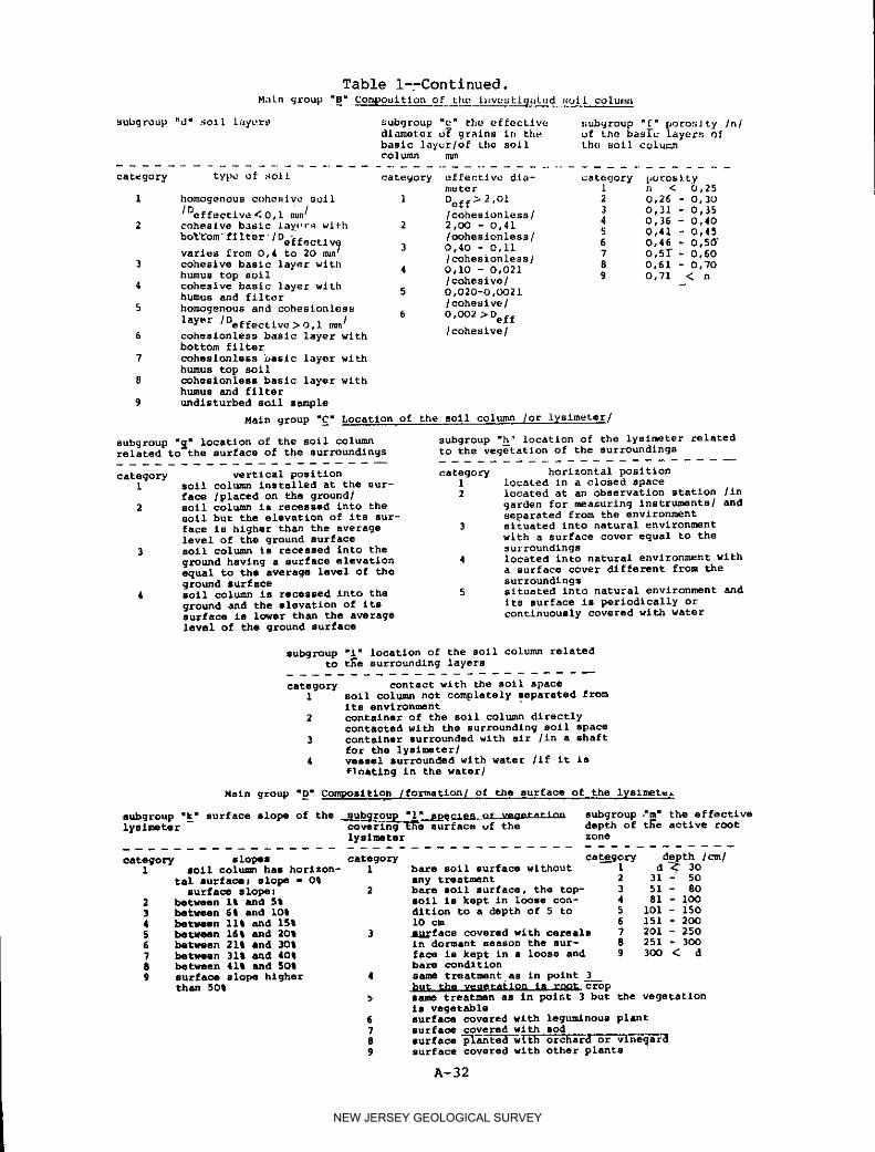
Table l-rContinued.
Mats group "B" Compouitlon of the Invustl_ated soil column
subgroup "d" soll layer_ subgroup "_" thu _flectivc subgroup .f. porosJty /n/
diameter 07 gr_ins in the of the basic layers ofbasic layer/of tho soll the soll columncol tuns m_
........................................................
category type of soll category effective dla- category [Jorosltymuter I n < 0,25
1 homogenous cohesive soll ] Dof f>2'Ol 2 O,26 - 0,303 0,31 - 0,35
/Deffectlva<O,i _/ /coheslonless/ 4 0,36 - 0,402 coheslve basic lay.,.-s with 2 2,OO - O,41 5 O,41 - 0,45
bo_t_m'f_Iter /Perfectly /ooheslonless/
varies from 0,4 to 20 _a? 3 0,40 - O,ii 6 0,46 - 0,5_7 0,5[ - 0,60]cohesionless/3 cohesive basic layer with 4 O,IO - O,O21 8 0,61 - 0,70
humus top soll /cohesive/ 9 O.71 < n4 cohesive basic layer with 5 O,O20-o,OO21humus and filter
5 homogenous and coheslonless /cohesive/
layer /Deffectiv e>O,l mm j 6 0,002 •Deff
6 coheslonless basic layer with ]cohesive/bottom filter
7 coheslonless basic layer with
humus top soil8 coheslonless basic layer with
humus and filter
9 undisturbed sell sample
Main group "C" Location of the sell column /or Iysimeter/
subgroup "_" location of the sell column subgroup "h" location of the lyslmeter relatedrelated to the surface of the surroundings to the veg_tatlon of the surroundings............................................
category vertical position category horizontal position1 soll colum_ installed at the sur- l located in a closed space
face /placed on the ground/ 2 located at an observation station _In2 sell column is recessed into the garOen for measuring instruments] and
sell but the elevation of its sur- separated from the envlron_nt
face is higher than the average 3 situated into natural environmentlevel of the ground surface with a surface cover equal to the
3 sell column is recessed into the surroundings
ground havlng a surface elevation 4 located into natural environment with
equal to the average level of the a surface cover dlfferent from theground surface surroundings
4 soil col_mn is recessed into the 5 situated into natural environment and
ground and the elevation of its its surface is periodically orsurface is lower than the average continuously covered with water
level of the ground surface
subgroup wl" location of the sell colunm relatedto t_e surrounding layers
........................
category contact with the sell space
1 sell column not completely separated fromIts environment
2 container of the soll column directlycontacted with the surrounding sell space
3 container surrounded with air /in a shaft
for the lyslmeter/4 vessel surrounded with water /if it is
F1nating in the water/
Main group "D" Composlklon /formatlon_ of the surface of the Iyslmet_.
subgroup "k" surface elope of the ___sub_qu_ "I_gEA_JL or I_C _e^eln" subgroup ."m" the effectivelyslmeter- coverlng-_e surfac_ uf the depth of t_e active rooh
lyslmeter zone...............................................
oohegors slopes _othgo_ ca_.g_rydd_t_o/_11 IOII COlU=n has horizon- 1 bare sell surface without
tel luffed! slope l O_ any treatment 2 31 - 50surfacesloper 2 ba_e sell surface,the top- 3 51 - 80
2 between It and 5t sell is kept in loose con- 4 81 - IO03 between 6t and IOt dltion to a depth of 5 to 5 I01 - 1504 between llt and 15% I0 cm 6 151 - 2005 between 16t and 20_ l _face covered with cereals 7 201 - 2506 between 2lt and 30t in dormant season the sur- 8 251 - 3007 k_t_en 31% and 40t face Is kept in a loose and 9 300 < d8 between 41t and 501 bar_ condition9 surfaoe elope higher 4 same treatment as in point !_
than 50t but the veue_a_icn is root cropsame treatnmn as in point 3 but the vegetationIs vegetable
6 surface covered with leguminous plant7 surface covered with sod8 surfac.ep--l_nted with orchard or vineyard9 surface covered with other plante
A-32
NEW JERSEY GEOLOGICAL SURVEY

Table 1--Continued.
Muin gruup "_" WJt.,* b,JI.,,,,'cof flit:[_SI[*_C_
subgroup "n" uurfacu runoff subgroup "o" watcrtabl_
category category
I bolh incoming _lr_d uL:t[ l,_|l_y runoif l drained sell colu._ without permanentat,! _xclu,lcd water table
2 incoming rui_off *:; ,:xc]uddd but tb_ 2 regulation of watertJb]e according to
outflowil*9 runoff can occurc and a constant or a defined control programmuasured with a device being' able either to
3 both incoming and outflowing ru*huff dralne or to r_charge a changing amountare m_asured of water. Mod_lllng the ilorlzontal
4 both incoming and outflowlng runoff groundwater flow in the device the
can occurs but not measured depth of _hreatlc surface is measure_3 equlpmen6 w_Ich produces constant water-
table with recharging and dralnaging
changing amount of water4 watertable regulation accordlhg to a
defined program with an equipment
recharging or dralnaglng changing _Untof water
5 equipment for measuring the elevationof water table without influencing th_development of it
subgroup "_" water recharge of the sell coltimn........................
category
l only natural recharging from precipitation2 artificial recharging through the
surface with sprlnklin_ irrlqatlon
3 artificial re.large .of the. sql _ golumnwith flooding
4 recharge of'water artificiallydirectly into the gravitational ground-water space
Main group "_" Methods of basic measurements of l_slmeter
subgroup m[. method Of measuring the sloped subgroup #s" Method Of sell molsturo
amount of water Masuremen_B
oetegory measuring method category meaauring method
i weighlng the sell column by llfting 1 there is no soil moisture measuremmn_the cointalnel-lfrom lta shaft/_wbich at all
has no devlce for water table 2 weighing /the determination of the
regulation difference in welght between an o%_n2 weighing with scales installed on dry and wet soil sample_
the container which Is not supple- 3 measuring the moisture content with
_nted with a _vlce foe the regu- electric resistivityfallen of watertable 4 measuring the moisture co.tent with
] measuring the /liquid/ pressure electric capacitor
change of the hydraulic /Jack/ system 5 MAsurlng the moisture content withsupporting the conrainer which is not n_utron probesupplemented with a device for the 6 measuring the moisture content withrogulatlon of water table the combination of electric
4 _Ighlng method according to point I resistivity and neutron probebut the colntalner is installed with 7 determination of sol1 moisture content
-M0te_ table _9_etinq device , _. with other suitable method5 weighing method according to point 2
but the cointalner is installed withwater table regulating device
6 Weighing method according to point ]but the aolntainer is installed with
water table re_ulatln_ device
? measurlng the water volume recharg-ing and drelnaging the soil columnby estimating the difference betweennatural recharge /precipitation/ and_urfa_ runoff
sUbgroup "t" period of basic measurements".....................
category periodl continuous registration of data2 periodical measurements several
times within an hour3 periodical measurement several
times within a day but not morefrequently than an hour
4 periodical measurement severaltimes within one decade but notmore frequently than one day
5 periodical meas_Iement not more_f[pO_ent|y than ono deck_
6 irregular observations
A-33
NEW JERSEY GEOLOGICAL SURVEY

Table 1--Continued.
Maln group "G" $upplem_ntar_ n_asurem_nts
s_bgroup "_" Neteorological measuremonts subgroup "v" _gronomicel measurement/contlnulty o_ oDservatlons ant] ae tesst /denslty of stand crop WhLCn is _quul to _ne
_y-@e_tlffon o_ measurements is numbed-of plants within a unlt area, supposed tonecessary/ he known/...............................................
category categoryI there Is no meteorological obser o i there is no agronomical n_asuren_nt at
ration at all all
2 _asuren_nt of precipitation 2 weighing the crop only In the final
3 measurement of air temperature phase of growthand precipitation 3 weighing only in the final phase of
4 measurement of relative hum/nidlty growth the dry matter of plants e_rg-of air and precipitation Ing above the ground s_rface
5 measurement of wind velocity and 4 weighing the total dry matter Of pla_t_precipitation only in the final phase of growth
6 measurement of tempezatura and /comprising roots and the part of plan£sre_atlve humidity of air as well emerged above the _surface/
as _reclpltatlon 5 contlnous weighing the dry matter of7 measurement of wind velocity a_d plants emerging above the ground surfac8
_elatlv_ h&_mldlty of air as well 6 continous welghlng the dry _atter andas precipitation the surface area of the leaves of
8 measurement according to point 6 plants emerging above ground surface
completed wlth wlnd velocity 7 contlnous weighing of the total dry
9 m_eomologicsl observations at a matter of plantsI order station /measurements 8 contlnous welghlng of the total drylisted In point 8 supplemented matter plants and the surface area of
wlth water surface evaporation-' leaves-using mA" and GGI 300 type pans-,sunshine duration, soll tempera-
ture of the upperlying layers,radlatlon e.c.t, observations!
subgroup "_" other measurements
category measurementI _epth and surface sree measurement of stagnant
pool8 occurlng on the surface of the investlgate_
Boll _olumn after water recharging processes_nrough the surface8o_1 temperature measurement in the lyslmeter
3 alr temperature measure_nt in the closed shaft
where lysl_eter Is recessed In4 measurlng the chango In po_oslty of the soll column
In • profile
5 Jol_t-mmasurem_nt of factors listed in point I and 26 " • 1,2 and 3
: : : land,8 2 and 39 1,2,3 and 4
A-34
NEW JERSEY GEOLOGICAL SURVEY
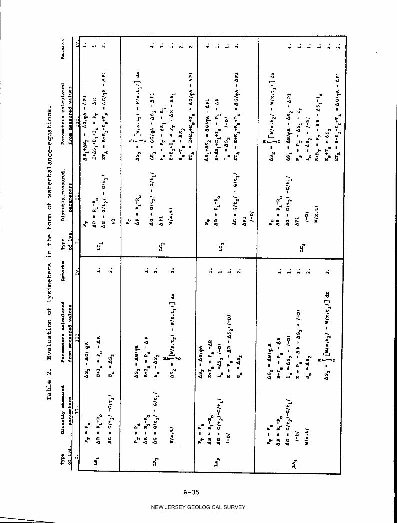
A-35
NEW JERSEY GEOLOGICAL SURVEY

I
I _ II @m
o, g_._, =o, io ,."_2 =o,
li_ll _ .,.i ._.i_ l _ . l I il II II l
c:0
I
oJ,-4,Q
E.., , ,_
_ ,_-o. o. _, % ._ _ '_ I
I i _ I l
_ l,,q ,._ ,_ _I _ _,_ _ _,-i_ r,d
_..,._ , ,.,,o_ I_..-,o._ o _o _ =o "-
.,d ..,I_ 4.1 II S_ .,=I II
I
f f
A-36
NEW JERSEY GEOLOGICAL SURVEY

..... . ....
I I
s I
_'_' % ? _ ,
I I
_,4 _ _ll-i J_14 i_l.l I _-s _ m _Id_.4 ..,lid4_
= .. , ,_.._. _ _ ,=o o . . ,
4J
II
,-,4e_
N A
I _ I IQ
, "2. , 1,.l
, _ _ , -?' < Q' , , . ? , _ ,:, o ,_ , ',.,_ ._
i I
7 3 ,,:o_ _ -" "- ' a
""_g°_,.o- !2 ' =II1= _ II
I i I I i _O_ll. ' I I , . "='"_1 q ' I
A-37
NEW JERSEY GEOLOGICAL SURVEY

•"4 I E,_ I ,_ Li31_'_
•<_ '<1 _ "<1 Id
.I | I II II I
*,'44J
o _ _II
1%1
r-t
, { _ , _
' _ -. -_
I l'_ i O.I I I 0 _l
,_ Id ll, ld Id
- Z gz z '_
N.o. o _ .o_I I I
A-38
NEW JERSEY GEOLOGICAL SURVEY

II
7:/° _
I'o." " • . .
o ° _
__ ,... _ _
Water table V /4 I io 9
Oo oz N
Figure i. Physical model representing hydrological processes occurring inthe unsaturated zone.
A-39
NEW JERSEY GEOLOGICAL SURVEY

Totnl porosit_l
Figure 2. Interpretation of field capacity and gravitational porosity asfunctions of the elevation above the watertable.
A-40
NEW JERSEY GEOLOGICAL SURVEY

pf =/og5
PI
P
3
2
, N.%,
'tt
a
0 lO 20 3oW%_0
Moi_fure in percenf by volumeFigure 3, The general form of a pR curve determined with point measurements,
A-41
NEW JERSEY GEOLOGICAL SURVEY

A-42
NEW JERSEY GEOLOGICAL SURVEY

A-43
NEW JERSEY GEOLOGICAL SURVEY

Supplement_rgrechargefor theexternalspace
Q(t) measuredrechargeof the/ntersalsp_ce
._oublecglmder
Surfoce 'h -:, 0
Figure 6. Hydraulic conductivity of the unsaturated zone, as the function ofsaturation.
A-44
NEW JERSEY GEOLOGICAL SURVEY

o _ _ _
,-4.r=:
_ •
//_z./l/qDazuJada4qDlad,y/ qy o .e_
_ "--..__ -_- _._
,, _ /,¢__ _o
N/I/q/;a/.u,Jad a,_.l;DlaJ>llZly
A-45
NEW JERSEY GEOLOGICAL SURVEY

Figure 8
A-46
NEW JERSEY GEOLOGICAL SURVEY

MODEL ECOSYSTEM STUDIES : MODELS OF WHAT?
by
Drs. GEORGE CLAUS, KAREN BOLANDER and Pml'zR P. MADRI
Columbia University Seminar on Pollution and Water Resources, and
Department of Microbiology, Brunswick Hospital Center
Amityville, New York
B-I
NEW JERSEY GEOLOGICAL SURVEY

The concept that most of the chlorinated hydrocarbon insecticides are
highly resistant to biodegradation and are retained in the environment for
considerable time periods, whereupon they become sequestered in living orga-
nisms and subsequently magnified in both terrestrial and aquatic food chains,
is one which has been so frequently repeated during the last decade that it
appears to have become almost universally accepted. For the most part, this
thesis rests on a large number of correlative field studies, the enumeration
of which is beyond the scope of this paper. However, there have been
attempts to duplicate this phenomenon under controlled laboratory conditions,
mainly through the so-called "model ecosystem" approach. These studies have
been carried out primarily at the University of Illinois by Metcalf and his
coworkers, although some other works relevant to the topic are known (for
instance, Reinert, 1972). In the present review we shall focus on the exper-
iments of the Illinois investigators, reported in the following papers:
Kapoor, Metcalf, Nystrom, and Sangha, 1970; Metcalf, Sangha, and Kapoor,
1971; Kapoor, Metcalf, Hirwe, Lu, Coats, and Nystrom, 1972; Metcalf and
Kapoor, 1972; Kapcor, Metcalf, Hirwe, Coats, and Khalsa, 1973; and Metcalf,
Kapoor, Lu, Schuth, and Sherman, 1973.
The original impetus for undertaking the the model ecosystem experiments
seems to relate to the search for substitute chemicals which would retain the
advantageous residual action against target insect species associated with
DDT and other widely used pesticides of the organochlorine group, but which
would be more "biodegradable"--especially by members of the vertebrate
phylum. During the past few years Metcalf and his coworkers have synthesized
a considerable number of "DDT analogs" and have tested these both for their
insecticidal activity and their biodegradability (Metcalf, 1973). The
behavior of these compounds in the model ecosystem has been compared with
that of such insecticides as DDT, DDD, aldrin, dieldrin, endrin, lindane,
hexochlorobenzene, etc., as well as with non-insecticidal but persistent met-
abolic products such as DDE.
The claims made regarding the efficacy of the model ecosystem as a
screening technique for the evaluation of new pesticides and as a simple,
practical, replicable methodology for determining the environmental effects
of pesticides now registered for use are presented strongly in all of the
publications emerging from the work of Metcalf and his coworkers. Since
these claims appear to have been accepted without critical scrutiny by impor-tant decisionmaking bodies and even by scientists who defend the need for
continued use of the well known chlorinated hydrocarbon insecticides for
increases in food productivity or for disease vector control programs, it was
felt that a critical evaluation of these publications and an attempt to par-
tially replicate the findings of the Illinois group would be fruitful. The
following, then, is a report of a review of the studies, and the results of
our experiments bearing on confirmation. Our evaluation centers broadly on
four topics: (i) the nature of the system, its components, and the tech-
niques employed by Metcalf and his coworkers; (2) results of ouz algal growth
studies; (3) the reported findings per se of the Metcalf group; and (4) theconclusions and claims put forth by the investigators.
The System
The model ecosystem as first described by Kapoor et al. (1970) consisted
of a maall glass aquarium 10 X 12 X 18 in., containing a shelf of 15 kg
B-2
NEW JERSEY GEOLOGICAL SURVEY

washed white quartz sand and 12 1 "standard reference water." The sand is
steeply sloped in such a way as to provide a small above-water portion where
Sorghum halpense can be grown. The Sot@hum seeds are planted on the first
day of the experiment. The following members of the test ecosystem are
introduced into the aquatic portion of the aquarium on the same day: phyto-
and zooplankton from old aquarium water, the filamentous green alga
Oedo_onium cardiacum, Daphnia magna, and Ph[sa sp. snails. The water is con-tinuously aerated with a pump, and the system is kept at 26Oc with 12 hour
exposure to 5000 ft. candles in an environmental plant growth chamber. After
20 days, when the Sorghum reaches about 6 in. height, 5 mg of a radiolabeled
insecticide is applied to the leaves of the plant. Ten larvae of the salt
marsh caterpillar Estigmene acrea are placed in the aerial portion of the
aquarium. The caterpillars completely devour the plants, and their feces--
containing radiolabeled compounds--then contaminate the aquatic part of the
system. After 26 days, 300 Culex quinquefasciatus mosquito larvae are addedto the tank, and after 30 days, three Gambusia affinis fish are placed in the
water. The experiment is terminated after 33 days, at which time weighed
samples of fish, snails, mosquito larvae, algae, and water are removed,
extracted, and assayed for radioactivity by a series of techniques (to be
described later).
In the 1971 publication of Metcalf et al., some further details are given
about the model ecosystem, with two specific changes (quantity of water and
size of aquarium), and certain discrepancies in description. The size of the
aquarium is there said to be 10 X 12 X 20 in. with 180 in.2 surface (sic),and only 7 liters of "standard reference water" are used. It is stated on p.
710 that a plexiglass cover ii X 12 in. is placed over the aquatic portion of
the chamber, and on the following page that ". . . the 4 in. open end of the
aquarium covered (sic) with copper screen to confine the insects" (Metcalf e__tt
al., 1971, p. 711). No explanation is offered as to what might cover the
missing 4 inches (12 + 4 = 16; the total length of the aquarium is stated to
be 20 in.). The sand-water system is equilibrated for one day (day 0) before
the introduction of any organisms. On day i, 50 Sor@hum seeds are planted in
5 rows, and several ml of old aquarium water, a "few" strands of Oedo_onium
cardiacum, 30 Daphnia magna, and 10 Ph[sa snails are added to the water. The
organismic composition of the old aquarium water is reported as follows:
among the identified diatoms are Navicula, Coseinodiscus, Diploness (sic),
and Diatomella. The zooplankton include the protozoa Nuclearia, Coleps,
Vorticella and Paramecium, and the rotifera Asplanchnopus, Notomatta (sic),Euclaris, and Scaridlum.
After 20 days, the Sorghum plants reach 4 in. height and are treated with
5 mg pesticide. The rate of application is said to correspond to about 1
lb./acre. On the same day, 10 5th instar larvae of the salt marsh caterpil-
lar are placed onto the dry sand, with the expectation that they will consume
nearly all of the treated leaves within 3 to 4 days.
After 26 days, when it is expected that the aqueous portion of the
aquarium should be contaminated with the radiolabeled compound through the
caterpillar feces, the leaf frass, and the caterpillar larvae themselves, 300
Culex pipiens quinc/uefasciatus larvae (here correctly named) are added to the
water. Four days later, 50 of the mosquito larvae are removed from the sys-
tem for analysis, at which time 3 Gambusia affinis mosquito fish are placed
in the water. These are expected to eat the remaining 250 mosquito larvae
B-3
NEW JERSEY GEOLOGICAL SURVEY

and the 30 Daphnia. "The experiment is terminated after 33 days, when
weighed samples of the organisms were (sic) examined for radioactivity...
Samples of sand are counted for radioactivity, together with duplicate l-ml
aliquots of water taken from the aquarium at i, 3, 7, 14, and 28 days after
treatment of the Sorghum" (Ibid., p. 711).
There are four problems with this description which are of more import
than the confusing numbers referring to the surface dimensions of the aquar-
ium or the misspellings of generic names and uncorrected grammar. First, ofthe four diatoms supposedly identified, two--Coscinodiscus and Diatomella--
are not fresh water species. One would therefore hardly expect them to bepresent in old aquarium water. Secondly, while it is mentioned in all of the
publications that samples of various organisms and other elements of the
system were weighed, data regarding these weights are not presented.
Calculated distributions of each radiolabeled compound under test, together
with its breakdown products in certain of the organisms and in the water, are
presented in the form of tables but are always expressed in terms of milli-
gram per kilogram, and without information on the absolute quantitiesinvolved, any attempt to scrutinize the investigators' findings is rendered
exceedingly difficult. Thirdly, even though residue values in the sand were
said to have been determined, in none of the publications are those values
reported. Lastly, since both publications describing the operation of the
system state that the experiment is terminated "after 33 days," and since it
is said that approximately 30 Daphnia magna are added to the model ecosystemat the be@inning of the experiment (Metcalf et al., 1971), one is left with
the clear impression that the duration of the entire experiment (from day i)
is 33 days. On the other hand, samples of sand and water are apparently
still being extracted and assayed on days 34 and 48 (14 and 28 days af'ter
treatment of the Sorghum, which takes place on day 20). If the water was notextracted for chemical and radioactive assays on the same day as were the
organisms, conclusions drawn from the experimental results (which are based
on proportions of the investigated compound in water and in the organisms)
would be completely invalid. This dilen_a can only be resolved if one pre-
sumes that what the authors meant to say is that the experiments are termi-
nated 33 days after treatment of the Sot@hum leaves with an insecticide, or,in other terms, that the duration of the entire experiment is actually 53rather than 33 days. Nowhere, however, do they so state.
Chemical and Radioassa[ Techniques
In addition to the model ecosystem studies reported in these publica-
tions, the investigators performed several other experiments in attempts to
elucidate the metabolic pathways of different pesticides in the salt marsh
caterpillar, in houseflies, and in mouse liver homogenates. They also
studied the elimination of the compounds in urine and feces of mice following
oral dosing of the animals. We do not intend to deal with these questions in
the following discussions, except where comparison between the results
reported in different publications are pertinent to evaluating the accuracyof radiotracer methods employed. Otherwise, we shall restrict our remarks to
those topics which bear directly on the model ecosystem studies.
From the scanty descriptions in the several publications of the method-
ologies one arrives at the following rather imprecise understanding of the
chemical and radiotracer analyses used by these investigators (given slight
B-4
NEW JERSEY GEOLOGICAL SURVEY

variations dependent upon whether the starting material was a 14C or a 3H
labeled compound).
i. l-ml aliquots of water were periodically assayed in "cocktail D" (100
g naphthalene and 5 g pPO in dioxane to make 1 liter) by scintillation
counting.
2. Unspecified quantities of the organisms and water in the system were
assayed at the termination of the experiments for quantitative and qualita-
tive determinations of both parent compound and degradation products. All of
the publications refer back to Kapoor et al. (1970) for basic information on
the techniques employed; however, in two other papers there are summaries
given which are at variance with that of Kapoor et al. (1970) and even the
original description is far from being clear. For this reason we cite the
appropriate passages from the three papers in question. After termination of
the experiment " . .weighed samples of fish, snails, mosquito larvae, algae,
and water were removed and assayed to (sic) total radioactivity. These
samples were homogenized and extracted with diethyl ether, and both water and
ether layers examined by TLC to determine the qualitative and quantitative
nature of the degradative (sic) products present, using radioautography and
serial scintillation counting of the areas containing radioactivity" (Ibid.,
p. 1149). One page earlier the reader is informed that " .wherever animal
extracts were investigated, . . . all such extracts were "'cleaned up' before
chromatography by partitioning in acetonitrile petroleum ether 2:1. The
acetonitrile fraction was evaporated and the radiolabeled metabolites taken
up in acetone or ether for application to the TLC plates" (Ibid., p. 1148).
In the publication of the year following, on the other hand, where the
details of the model ecosystem are treated, the chemical methodology is as
follows: ". -- .weighed samples of the organisms were examined for radio-
activity. (There is no mention of the water.) The samples are homogenized
in water and extracted with equal volumes of diethyl ether. Both layers are
examined by TLC to determine the qualitative and quantitative nature of the
radiolabeled products with use of radioautography and scintillation counting
of serial sections (sic)" (Metcalf et al., 1971, p. 711). At this time the
acetonitrile petroleum ether "clean up" procedure is not mentioned, and the
impression is that only aqueous extracts and those obtained with diethyl
ether were assayed. By 1973, the procedure is outlined in an even less
likely fashion: "After 33 days. . .the experiment was terminated, and the
amount and nature of the 14C determined by homogenization of the organisms,
extraction with acetonitrile, TLC autoradiography, and liquid scintillation
counting" (Metcalf et al., 1973, p. 36). From this one would deduce that the
extraction was carried out with acetonitrile, although this is hardly prob-able since the chemical is water miscible.
3. The next step in the procedure seems to be the separation and idenfi-
fication of the parent compound and the different metabol.ites by applying
unspecified quantities of the extracts to (apparently) three sets of silica
gel TLC plates which contained fluorescein (Kapoor et al., 1970), specifi-cally described in a later paper as fluorescent ma---rke--_E. Merck GF-254
(Metcalf et al., 1973). Non-radioactive labeled parent compounds and model
metabolites were cochrematographed with the "unknowns" in the extracts. The
visualization of the spots after the development of the TLC plates in the
appropriate solvents was achieved either through the quenching of fluores-
cence or by spraying with selected chromogenic agents. In order to localize
B-5
NEW JERSEY GEOLOGICAL SURVEY

the unknowns, autoradiography was used by applying No-Screen( R ) X-ray film
(Eastman Kodak) to the plates for unspecified periods of time.
4. After identification of the compounds in the extracts through the
development of the X-rays, the appropriate spots (i cm2 or more) from the
plates were scraped into "cocktail D" for quantitation by liquid scintilla-
tion counting.
Although the determination of total radioactivity in animal tissues was
carried out by Schoniger combustion technique for tritium labeled compounds,
all other aspects of the separation and quantification of the metabolites
were evidently the same as with 14C labeled pesticides. From Kapoor et al.
(1970) it would seem that the tritium labeled compounds were counted, after
TLC separation, in "cocktail D," while "3H cocktail" was used only for the
oxygen combustion procedures. (.3H cocktail" consists of 200 g naphtha-
lene, 10 g PPO, and 0.25 g POPOP in dioxane to make 1 I.) The authors
state: "The relative proportions of various radiolabeled metabolites (from
the previous paragraph, apparently including 3H labeled methiochlor) were
determined by scraping 1 cm2 or other appropriate sections of silica gel
from developed TLC plates into 'cocktail D'" (Kapoor et al., 1970, p. 1148).
From the 1971 Metcalf et al. paper, on the other hand, one is led to under-
stand that the scintillation counting of 3H labeled compounds removed from
TLC plates was carried out in "3H cocktail." Matters are made more con-
fusing since, on the same page, it is stated: "The general methods for
preparation and evaluation of radiolabeled samples have been described in
detail by Kapoor et al. (1970)" (Metcalf et al., 1971, p. 710).
The Food Chains
The food chains involved in this microecosystem are described in two of
the publications (Metcalf et al., 1971; and Metcalf et al., 1973). While at
first perusal the proposed food chains appear similar, there is also an
important discrepancy in these two descriptions. In the 1971 publication,
the food chain pathways are listed as:
" (i) Sorghum _ Estigmene (larva)
(2) Estigmene (excreta) P Odeo_onium (algae)
(3) Odeo_onium P Ph[sa (snail)
(4) Estigmene (excreta) P Diatoms(5) Diatoms _ Plankton
(6) Plankton , Culex (larva)
(7) Culex b Gambusia (fish)"
(Metcalf et al., 1971, p. 711.)
In 1973, however, a modification is instituted which seems to indicate only
two basic aquatic food chains: from Oedo_onium to Ph_sa; and from plankton
to Daphnia to Culex to Gambusia. The later version is rather questionable,since it is highly improbable that mosquito larvae will consume Daphnia.
There is, in addition, one much more important problem with the presumed
food chains in this system. In several of the publications it is stated that
both Daphnia ma@na and Physa snails are introduced on day i, or at the same
time when the "few strands" of Oedo_onium cardiacum and the "few ml" of old
B-6
NEW JERSEY GEOLOGICAL SURVEY
aquarium water are added to the aquatic portion. Under such conditions, it
would seem rather unlikely that the Daphnia would survive, even without the
presence of the pesticide (applied only after day 20), since they, like other
mezoplanktonic forms, require up to five times their body weight in food per
day (Hartman and Claus, 1971), and would certainly not obtain this from a few
ml of old aquarium water containing microzoo- and phytoplankton.
Furthermore, it seems unlikely that any substantial amounts of algae would
grow in the presence of the 10 snails--animals consuming from 2 to 4 times
their body weight in food under optimal conditions. This is particularly the
case if the investigators were indeed working with Oedo_onium cardiacum,
since all members of this green algal genus are relatively slow-growing
forms. In view of the fact that two of the diatoms mentioned as being
present in the old aquarium water were obviously misidentified and also
considering the rather curious fact that only diatoms were described as
present in the water, one might suppose that the investigators were working
with some other filamentous green alga exhibiting a faster growth rate.
Given the voracious appetites of the snails, however, it is questionable that
any filamentous green alga would produce enough biomass in 53 days to permit
proper quantitation of the minor metabolites which they accumulated by theend of the experiment.
These doubts about the viability of the Daphnia and the appropriateness
of the alga--_snail food chain, led us to undertake some experiments designed
to replicate as closely as possible the first aspects of the model ecosystem
studies of Metcalf and his coworkers. These experiments, the results of
which are reported below, tested the simple food chains of microplankton-_
Daphnia and filamentous or coenobial green algae--_Planorbis.
Culture Experiments
The test containers consisted of 10 2 liter cylindrical glass beakers,
Kimax(R) (13 cm diameter, 19 cm height). Carefully washed white quartz
sand (i kg) was placed into each of the beakers, and 1 1 "standard reference
water" of Freeman, as used by Metcalf et al. (1971) was added. (Constituents
in mg/l: MgS04, 36.4; K2S04, 0.135; CaCI2, 14.0; NaHC03, 25.0;
NH4N03, 3.0; K2HPO4, 0.78; CaC03, 57.7; NaSi03, 23.6; FeCI3,
0.81; prepared as 6 stock solutions. Solubilization of CaCO 3 was achieved
by bubbling CO 2 through the stock, which also elevated the pH of the final
"reference water" to 7.9.) After one day of equilibration, the film formed
on the surface of the water was carefully removed with blotting paper. The
water occupied an approximate 8 centimeter height in the beakers above the
sand. These levels were marked and maintained throughout the experiment by
adding "reference water" to compensate for loss by evaporation.
Each beaker was inoculated with 3 ml of "old aquarium water" and also
with a 1 cm2 scraping from the wall of the aquarium, containing periphy-ton. The weight of the microplankton in the aquarium water was established
in the following manner: 10 ml of Millipore(R) (pore size 0.45_ ) filtered
water was weighed in a beaker on a Mettler H30 analytical balance, and
thereafter, 10 ml of aquarium water containing microplankton was filtered
through a preweighed wet Millipore filter, as above, which was then added to
the beaker, followed by another weighing. The weight difference, after sub-
tracting that of the added Millipore filter, was less than 0.01 mg, which
would indicate that in 1 ml of aquarium water, the weight of organisms is
less than 0.001 mg. A quantitative cell count was performed on the aquarium
B-7
NEW JERSEY GEOLOGICAL SURVEY

water, using a Spencer(R) Neubauer Bright-Line hemocytometer, and the total
number of cells per ml was established as ca. 980. Since the calculated
average weight of a planktonic algal cell is about 1 X 10 -9 g, i000
cells/ml would weigh 0.001 rag, a figure in relatively good agreement with
that obtained through the weighing method. The weight of a 1 cm 2 scraping
of periphyton was established as 0.14 rag. Two beakers each were inoculated
with the following green algae: Clado_hora _lomerata, Bydrodic tyon
reticulatum, Mou@otia sp., Odeo_onium fra@ile, and Ulothrix zonata. The
algae were derived from the stocks of Carolina Biological Supply Co.,
Burlington, N.C.
Five of the beakers, each containing a different species of green algae
under test, served as controls, while the other five were designated as the
experimental containers. In the latter, Daphnia pulex and Planorbis sp. were
added on day 1 in order to determine differences in algal productivity in the
presence of grazers.
Clado_hora @lomerata: 20 large branched plants (up to 5 cm in length)harboring heavy growth of epiphytes were selected under a dissecting micro-
scope and transferred into two beakers (i0 in each) holding i0 ml of water,
which had been previously weighed. After reweighing the beakers containing
the plants, the weight of the 10 Clado_hora in the two beakers was estab-
lished as 8.3 and 7.8 mg, respectively. The plantS were then placed into the
experimental end control beakers containing sand, standard reference water,
microplankton, and periphyton.
H_drodictyon reticulatum: 20 nets, approximately 0.5 cm in length were
selected +under a dissecting microscope and 10 each were placed into the
beakers containing the elements described above. The weight of the plants
could not be determined directly; therefore they were calculated on the basis
of average cell dimensions and the number of cells in the coenobium, using
30 _ length, 10 _/ width, and approximately 6,000 cells in each net.
Mou@otia sp.: 20 strands were separated under the dissecting microscope
and the weightS of the plantS were calculated,, using an average length for
the filaments of 10,000 _ and a width of 12 ]/. Ten filaments each were
placed into the beakers as previously described.
The same procedures were carried out with Oedo_onium fragile, where the
average length of the filamentS was established as 20,000 _/ having a width of
10 _ and with Ulothrix zonata, which had an average length of 6,000 _/ and a
width of 8_ .
Thirty Daphnia pulex were transferred into a beaker holding 1 ml of water
which had been weighed. After reweighing the beaker with the Da_hnia the
weight of the cladocerans was established. This procedure was repeated five
times, and the five experimental beakers containing algae and microplankton
were then seeded with 30 Da_hnia each.
Ten Planorbis sp. were placed into a beaker containing i0 ml of water
which had been weighed and the weight of the snails established through
reweighing the container. The snails were selected so that the total weight
of the ten animals should come as close to two grams as possible. Again, the
B-8
NEW JERSEY GEOLOGICAL SURVEY
procedure was repeated five times, and ten snails were placed into each ofthe experimental beakers.
Both the Daphnia and the snails were purchased from a local aquariumsupply store.
A list of the planktonic organisms together with the counts of the domi-
nant forms, as well as lists of the periphytic and epiphytic forms, is given
in Table i. Where obvious periphytic forms were found among the plankton,
they were enumerated only under the heading "periphytes." The zooplankton
were exceedingly sparse, with the following organisms found in small num-
bers: St_lonichia pustulata, Oxytrycha sp., and Holophr_a discolor. Amongthe periphyton, scattered individuals of Vampyrella lateritia, Tokophrya
lemnarum, Vorticella sp., Stentor coeruleus, and Stephanoceros sp. were seen.
The five experimental and five control beakers were placed into a walk-in
incubator kept at 26Oc, and they were exposed to 12 hour illumination
daily, with GroLight(R) fluorescent lamps of 5,000 lux. Each beaker was
covered with an hour glass resting on a wire triangle and aerated with a
Little Giant(R) air pump. From day 20 to the termination of the experimenton day 33, 20 mg daily of TetraMin(R) fish food was added to the water of
both control and experimental beakers in order to simulate the organic
enrichment originating from caterpillar excrement in the model ecosystemstudies.
On the 33rd day, when the experiments were terminated, plankton counts
were performed, and the weight of all surviving animals was either determined
directly or through calculations. Concurrently, the filamentous algae were
counted individually and their weight directly established, or, where they
were too few in number, determined by calculations. After removal of the
macroscopic organisms, the water from each beaker was filtered through a wet,
pre-weighed Millipere(R) filter (0.45 _ pore size) and the weight of theplankton was measured where possible. In those cases where most of the
microplankton had been consumed by the grazers, weights were calculated from
the microscopic counts. The entire internal surface of each beaker was
scraped with separate scalpels and the total weight of periphyton from each
container was established. Since the water-exposed surface of the beakers
could be calculated, the weight of periphyton could also be expressed in
terms of mg/cm2. Table 2 contains both the initial concentrations and
weights of the organisms or groups studied and their concentrations and
weights at the termination of the experiments.
Among the algae tested, only Cladophora yielded a biomas in the gram
range, and that only in the control. In the test series, in the presence of
grazers, neither the phytoplankton-periphyton complex nor the test plant
itself gave yields above the 100 mg range even with Cladophora. In all of
the experimental beakers, it was apparent that the grazers were starving.
Only a few Daphnia survived, and only in those experiments where adequate
epiphytic flora occurred on the test plants (Cladophora, Odeo_onium, and
Ulothrix) to provide nourishment for the cladocerans. Some snail mortality
also took place--probably due to starvation--although it is recognized that
snails are better able to tolerate long periods without adequate food supply
than are the smaller invertebrates. Hydrodictyon had been virtually devoured
by the snails by day 2, and this may account for the fact that the greatest
B-9
NEW JERSEY GEOLOGICAL SURVEY

loss of snails was observed in this experiment. In the Hydrodictyon, the
Oedogonium, and the Mougotia experiments, the periphyton were also almost
completely consumed by the snails. Relatively large numbers of Mougotia fil-
aments were found in the experimental beaker at termination (13,000), perhaps
reflecting the fact that this alga is not a preferred food organism forsnails.
It is well known that small aquatic grazing invertebrates can eat, under
optimal conditions, from 2 to 5 times their own body weight daily (Raymont,
1963). In none of these experiments was there sufficient food to nourish the
animals adequately. The voracious appetite of the grazers was best demon-
strated in the Cladophora experiment, where, at termination, the weight of
the plants was 5,344 mg in the control as compared with 83.6 mg in the exper-
imental beaker. Those Cladophora remaining in the experimental beaker showed
scarce branching in comparison with the controls, having been badly damaged
and partially eaten by the snails; hence their greatly reduced individual
weights.
In the Oedo_onium and the Ulothrix experiments, it seemed likely that thesnails would have consumed all of the filaments before termination had they
been able to locate them, since the animals were clearly without adequate
nourishment. In no experimental series did the snails exhibit the gain in
weight which would be expected after 33 days in an environment with an abun-
dant food supply.
It should also be remarked that although these experiments were initiated
using 10 plants of each test species on the assumption that the imprecise
phrase "a few strands of algae" used by Metcalf and his coworkers should be
interpreted as referring to a relatively small fihite number, there wouldhave been little difference in the quantities of algae obtained in 33 days,
with the snails present from the beginning of the experiment, even had 100filaments been used. The snails would most probably have consumed greater
quantities of the initially added filaments, still leaving only a few plants
able to reproduce during the course of the experimental period.
An additional corment should be made regarding the use of Oedogonium
fragile rather than Oedo_onium cardiacum in our growth experiments. It is
recognized that the latter species is about 5 times as large as Oe. fragile.
A substantial difference, however, between the two forms is that Oe. car-
diacum is a dioecious form, whereas O__ee.fragile is monoecious (Collins,
1928). With monoecious forms fertilization chances are far greater in a
thinly populated culture than are those with dioecious forms under similarconditions. Therefore, differences in final biomass will not differ substan-
tially between the two forms, since the faster sexual reproductive process in
the monoecious form w'll compensate for the larger size of the dioecious
organisms.
Although in the present culturing experiments beakers with only 1 liter
of water were used, instead of aquaria containing 7 liters, this fact will
not change the results with respect to final productivity, since these are
expressed in terms of ratios: milligram of algae, or number of planktonic
cells, per quantity of water.
B-10
NEW JERSEY GEOLOGICAL SURVEY

On the basis of these culturing experiments, it seems rather questionable
that the food chains postulated by Metcalf and his coworkers would be ade-
quately supportive for the members of the higher trophic levels (Daphnia,
Culex. Physa, and Gambusia) employed in their microecosystems. Furthermore,
it seems even less likely that in any of their experiments, adequate quanti-
ties of algae would have been available at the end point of the studies for
the investigators to separate, identify precisely, and quantitate minor meta-
bolic products of the different pesticides. For these reasons, we wish to
further scrutinize the techniques used and the findings reported by the
Illinois group from their various experimental series.
Remarks on Radiotracer Techniques
Since no data are given regarding the efficiency of the scintillation
counts it is necessary to turn to the published literature on radiotracer
methods in order to gain some idea about the appropriateness of the "cock-
tails" used in the counting series and of the efficiencies involved in
scraping portions of thin layer silica gel plates into scintillation vials.
"Cocktail D" is a dioxane-based counting fluid which contains no wave shifter
and no anti-freeze. "3H cocktail" does have a wave shifter (POPOP), but it
is also dioxane-based. Such fluids freeze at 12°C, and it seems therefore
that counting must have been performed at or above this temperature. It is
known that for every 10 degrees of temperature increase over 0Oc an
increase in "background noise level" of approximately a factor of 2 may be
expected (Wang and Willis, 1965). Although the investigators mention the use
of channels ratio technique for quench correction, the relatively high back-
ground noise in samples with low activities (to he discussed later) renders
the accuracy of such quench correction curves questionable.
A second factor to be taken into account is that the silica gel with the
radiolabeled compound adsorbed to it is scraped directly into the scintil-
lation liquid. A nonhomogeneous system will thus be established. There is
no reason to suppose that the parent compound and its metabolites will be
equally solubilized by dioxane. Quite to the contrary, it is almost certain
that only portions of the radiolabeled material will go into solution, while
other portions will remain adsorbed on the solid support. Bransome and
Grower (1970), using various solid supports and employing the channels ratio
technique, demonstrated that ". beta spectra of (14C), as well as
(3H), samples are shifted toward lower energies, and that external standard
channels ratios are completely inadequate for quench correction" (Bransome
and Grower, 1970, p. 404). Furthermore, as far as 3H labeled compounds are
concerned, they write: "Correction by CR for loss of (3H) would obviously
be statistically unreliable" (Ibid., p. 405). Indeed, in their samples, the
severe quenching of the tritium spectru_ caused by the presence of the solidsupport was such that most of their counts were below the detection thresh-
old. In their conclusions they state: "The disappearance of most of the
(3H) spectrum below the detection threshold prevented any reliable quench
correction by means of CR values, and made any assumption of constant effi-ciency very hazardous" (Ibid., p. 407).
McKenzie and Gholson confirmed these results, remarking in their intro-
duction: "Partial and/or variable elution of the labeled material(s) in the
vial can cause differences in the results obtained between duplicates of a
given sample or when comparing chemically different compounds which may
B-II
NEW JERSEY GEOLOGICAL SURVEY

behave differently in the same systems" (McKenzie and Gholson, 1973, pp.
17-18). They tested a counting fluid which was far superior to those used by
Kapoor et al. (1970)--one composed of 4 g PPO, 0.2 g POPOP, 400 ml absolute
ethanol, and 600 ml of toluene per liter--which would not freeze at 0oc and
gives a higher counting efficiency than dioxane due to toluene's 30% greater
excitation energy transfer. In spite of using this better "cocktail," they
did not find the recovery rate of radioactive material from a silica gel sup-
port to be satisfactory. When they used a special formulation referred to as
BBS-3 (Bio-Solv, Beckman Instruments, Inc.) in addition to their cocktail,
they were able to achieve about 90% recovery with 14C, but they still did
not find satisfactory recovery of tritiated compounds under most conditions.
A further element of uncertainty in the experiments of Metcalf and his
coworkers is added by the presence of the fluorescein marker in the silica
gel. The emission wave length of fluorescein is 520 nm, and that of PPO is
380 nm; thus excitation of the fluorescein in the sample may interfere con-
siderably with the final counting rate, acting in a manner similar to a sec-
ondar y fluor.
Summarizing what we have stated concerning the scintillation counting
methodology, the counting efficiency for the 14C labeled samples is
unlikely to be higher than ca. 40%, and that with tritium will certainly be
belGw 10%, when such scintillation fluids as the investigators' "cocktail D"
and "3H cocktail" are employed.
Similar problems would arise if 1 ml aliquots of water were assayed in
either "cocktail D" or "3H cocktail," as was evidently the case in all of
these experiments. The planktonic organimns present in the water will
produce considerable quenching, quite like that introduced by the presence of
a solid support.
An integral part of the radioassay techniques of these studies is the
identification of the metabolic compounds through autoradiography. Knowing
the amount of radioactivity in the starting material and calculating the
equivalent dpm's in the metabolites, it is possible to gain an impression of
the magnitude (or lack thereof) of the activities present. It is recognized
that ". _06 108 beta particles must strike each square centimeter
of X-ray film to produce optimal blackening. ." and further that
"... detectable blackening may occur as a result of 105 106 beta
interactions per square centimeter" (Wang and Willis, 1965, p. 147).
When, for instance, some of the metabolites of methiochlor are represent-
ed (Kapoor et al., 1970), where it is unquestionable that a 3H labeled
compound was under test, it is possible to calculate the approximate exposure
time required to produce even a faint image on the X-ray film. For some
metabolites, necessary exposure is in the range of 700 days. It would be
interesting to know the exposure times in these experiments, since they are
not reported. Granting a two year exposure, the selection of Eastman Kodak's
No-Screen(R) X-ray film still seems to be somewhat less than satisfactory,
as this film has been described as having poor resolution and a high back-
ground sensitivity (Wang and Willis, 1965, p. 146).
B-12
NEW JERSEY GEOLOGICAL SURVEY

The Dieldrin Experiment
Dieldrin has been selected from the 1973 publication of Metcalf et al.,
in which the results of model ecosystem studies of six different chlorinated
hydrocarbon pesticides are reported, for three particular reasons. First,
the specific activity of the original radiolabeled compound is rather
iow--1.03 mCi/mM. Secondly, a detailed list of metabolites in water and in
the test organisms is given in the authors' Table 2. Thirdly, in an unpub-
lished report by Metcalf and Kapoor (1972) treating the fate of aldrin and
dieldrin in the model ecosystem, certain information is supplied which is
missing from all of the published works.
As has been mentioned earlier, since the quantities used for extraction
of water and organisms for further analysis are not specified, it is neces-
sary to make certain assumptions in order to give some absolute value to the
data reported in terms of ppm. It is assomed arbitrarily that 1 1 of water
was used for extraction purposes at the end point of the experiment.
Although it is highly questionable that there could have been more than i0 mg
of Oedo_onium cardiacum present in the tank at termination, for these calcu-
lations we have granted a biomass of i00 mg of algae. We prestige that the
total weight of the snails is 2 g (200 mg each), even though the species is
unidentified, and we further assume that the investigators extracted the
whole 2 g. The average weight of Gambusia affinis is 2.1 g (Culley and
Ferguson, 1969), and we assome that all three fish were hc_ogenized and used;a total of 6 g. With these quantities, the conversion of the ppm values in
Table 2 of Metcalf et al. (1973) to nCi or dpm's is possible. These numbers
are compiled in Table 3. At 100% recovery and counting efficiency, several
of the metabolites in the algae and even in the fish are below detection
levels. Presuming a 40% efficiency, other figures will also represent cpm's
below detection, or would require unrealistically long counting times--in therange of weeks rather than hours (Freedman and Anderson, 1952). The question
must be raised why the investigators attempted to express these minor metabo-
lites in terms suggesting precise quantification, rather than merely indicat-
ing trace amounts when they were counting at levels which were unquantifiable.
At the low specific activity employed, counting of 1 ml aliquots of water
in "cocktail D" is also of questionable meaningfulness. The data from these
periodic counts are not reported in the published papers. However, in the
1972 preliminary note of Metcalf and Kapoor on the aldrin and dieldrin
series, the following sentence appears regarding dieldrin: "The radioactiv-
ity in the water phase rose to a maximt_n of 0.02 ppm by the 5th day and
declined to about 0.005 ppm over the duration of the experiment" (Metcalf and
Kapoor, 1972, p. 2). These values would indicate that on day 5, 54 pCi was
detected and that later (presumably day 15 or day 28), only 13.5 pCi. Con-
sidering the relatively low counting efficiency and the unknown variation in
the numbers of microplankton in 1 ml of water over the course of time,
whether or not these figures have any true meaning cannot be assessed.
Returning to Table 2 of Metcalf et al. (1973), there is one further
puzzle which applies equally to the reporting on the other pesticides tested
in this series. In the aqueous phase, substantial portions of materials
appear as unextractable residues. No methodology is described which would
shed light on how the quantity of this fraction was determined. There is,
B-13
NEW JERSEY GEOLOGICAL SURVEY

however, a strong suggestion that rather than making independent determina-
tions, the stn_ of the values for the parent compound and its metabolites was
simply subtracted from the value given for total 14C.
Concerning the dieldrin experiment, there are two further specific
matters related to the behavior of the organisms for which the authors offer
no explanation. It is stated: "The dieldrin application to the Sorghum was
more toxic than aldrin and the salt marsh caterpillars Estigmene acres, ate
the plants with reluctance" (Metcalf and Kapoor, 1972, p. 2). Were it indeed
the case that the caterpillar's "reluctance" to eat the dieldrin treated
leaves reflected its greater toxicity over that of aldrin, this interesting
observation should have been mentioned in the published version of this work
and elaborated upon, since nothing in the literature suggests that dieldrin
would have a higher toxicity to insects than aldrin. A more important prob-
lem reflecting directly on dieldrin toxicity is the discrepancy between the
findings of the aldrin and the dieldrin series with respect to mosquito
larvae mortality. In the dieldrin series, where its level in the water is
given as 0.0014 ppm, a footnote indicates that all mosquitoes were killed
throughout the experiment. On the other hand, in the aldrin series, where
aldrin's breakdown product dieldrin is given as 0.0047 ppm, the mosquitoes
not only did not die but managed to accumulate i.i ppm dieldrin. It seems
most peculiar that in the aldrin experiment the larvae should have survived
3.3 times higher dieldrin concentrations.
Reproducibilit_
Among the strong claims made by the investigators respecting the value of
their model ecosystem studies is the reproducibility of the results. They
write: "The ultimate purpose of the model ecosystem is to be used as a
single living unit for in-depth studies of environmental degradability. The
question of reproducibility of results is of considerable importance as even
this simple ecosystem is substantially more complex than any single experi-
mental animal or groups of animals. This factor has been evaluated by two
complete individual evaluations of the behavior of 14C-labeled DDT in the
model ecosystem with the results shown in Table II. The two studies gave
remarkably similar results, both as to distribution and accumulation of total
radioactivity in the components of the system and as to the quantitative bio-
degradability of DDT to DDE, DDD, and polar metabolites" (Metcalf et al.,
1971, p. 711). There is absolutely no question that two completely different
DDT model ecosystem studies ware involved, since in Kapoor et al. (1970) the
source of the radiolabeled DDT (specific activity 5.48 mCi/mM) was the World
Health Organization and the volume of water employed in the aquarium was 12
liters; whereas in Metcalf et al. (1971) the 14C-labeled DDT was supplied
by the Radiochemical Centre, Amersham, England (specific activity 5.48
mCi/mM) but the aquarium contained only 7 liters of water. Table II in
Metcalf et al. (1971) shows two separate experiments, with about 100% differ-
ence in total 14C results. However, in Table III of the same publication,
the DDT results clearly originate--not from the replicate experiment dis-
cussed--but rather from the earlier work of Kapoor et al. (1970). To the
reader, this becomes evident only if the two publications are placed side by
side and the figures of Table 6 from Kapoor et al. (1970) and those of Table
3 from Metcalf et al. (1971) are compared. The nlnnbers are identical to the
last decimal point. There seems to be no reason why the Metcalf et al. pub-
lication of 1971 should not contain detailed results of their replicate
B-14
NEW JERSEY GEOLOGICAL SURVEY

experiment, and there is no justification for reprinting the 1970 data in
their Table III, without clearly designating it as such. Any reader looking
only at the 1971 publication of Metcalf et al. would gain the definite
impression that the results on DDT reported in Table III refer to the repli-
cation experiment of 1971. Furthermore, even from the scanty materials
reported in Table II of the second publication, it is possible to question
the authors' claim that the two studies gave "remarkably similar results,"
since in experiment I (1971) the accumulation of total 14C in fish was 20.8
ppm, while in experiment II (1970), it was 54.2 ppm, giving a standard error
of 23.6--weli over 100% of the accumulation in the replicate experiment.
This matter of a 100% difference in the results of these two similar
experiments using the model ecosystem approach to study the environmental
fate of DDT is minor, however, compared with the markedly disparate findings
between the 1970 publication of Kapoor et al. regarding excretion of DDT in
mice (feeding experiments) with those of Kapoor et al. (1972) on the same
subject, employing different radiotracer techniques. In this connection we
cite two passages from the publications in question. In 1970, the authors
write: "DDT is eliminated very slowly (1.02% in the first 24 hr.), while
methiochlor (47.11%) and methoxychlor (98.3%) are eliminated rapidly. The
degree of polarity of the excretory metabolites is indicated by the ratios of
radioactivity in urine/feces which is 0.67 for DDT, 0.13 for methoxychlor,
and 0.19 for methiochlor. Over a period of ii days all of the methoxychlor
and 86.69% of the methiochlor were eliminated, as compared to only 4.3% of
the DDT" (Kapoor et al., 1970, p. 1150). The phraseology of the 1972 paper
is notably similar, but the numbers are remarkably different. Here it is
stated: "DDT was eliminated slowly (7.4% in the first 24 hr.), while methyl-
chlor (43.7%) and ethoxychlor (99.0%) (sic, 69%?) were rapidly eliminated.
However, over a period of ii days, 90.8% DDT had been eliminated compared to
73.7% for methylchlor and 77.5% for ethoxychlor, thus indicating that
although initially DDT has a much slower rate of elimination, it reaches the
level of the other analogs within 6 days. The degree of polarity of the
excretory metabolites is indicated by the urine/feces ratio, which is 0.47
for DDT, 0.69 for ethoxychlor, and 0.12 for methylchlor" (Kapoor et al.,
1972, pp. 3-4).
The most notable numerical discrepancy is that between 4.3% DDT elimina-
tion in 1970 and 90.8% in 1972 after ii days. These differences, which are
undoubtedly due to the use of the "more efficient" 02 flask combustiontechnique and to "N cocktail" (135 ml phenethylamine, 135 ml of methanol, 730
ml of toluene, 5 g of PPO, and 100 mg of POPOP), which is appropriate for
CO 2 absorption and high efficiency liquid scintillation counting, are notemphasized by the authors. The fact remains, however, that the results after
ii days in the 1972 experiment indicate a 2,100% error in the 1970 findings,
which were carried out by direct counting of diluted urine samples andwater-acetone extracted feces in "cocktail D." These extreme differences in
end results should have been pointed out by the authors and the investigators
should have been alerted to the limitations of their earlier radiotracer
techniques. Contrary to expectation, no mention is made of the irreproduc-
ibility of the first mouse excretion study and, in two publications appearing
in 1973 (Metcalf et al., 1973; Kapoor et al., 1973), the techniques used by
Kapoor et al. in 1970 are again described as the basic chemical and radio-
assay methodologies.
B-15
NEW JERSEY GEOLOGICAL SURVEY

The real significance, however, of the 2,100% error in the mouse excre-
tion studies goes beyond these experiments per se. It points to the proba-
bility that the radiotracer techniques applied in all of the model ecosystem
studies--as we have suggested earlier--were highly deficient, and that the
presented results are of doubtful validity. If the possibility of a 2,000%
error is considered and the dieldrin table is reexamined, for instance, all
dpm's which fall below the 10,000 level become questionable. The second
importance of the findings of Kapoor et al., 1972, with respect in particular
to DDT, is that by the llth day after ingestion the results indicate DDT to
have been more completely excreted than methylchlor, ethoxychlor, and methio-
chlor--compounds which the investigators, on the other hand, claim to be more
biodegradable.
(Another indication that the 1972 publication of Kapoor et al. involved
some improved techniques is the description of methods for isolating micro-
somal fractions to investigate enzymatic breakdown of radiolabeled
compounds. In 1970, Kapoor et al. state that microscmal pellets were precip-
itated from fresh Swiss mouse liver at 114,000 - 140,000 X g. Such speeds
are not appropriate for the separation of mlcroscmes° In 1972, Kapoor et al.
write: "The homogenate was centrifuged at 15,000 X g" (p. 3), a speed at
which one might actually expect to find the microsomes still in the super-natant. )
Some Theoretical Concepts: "Bioma@nification," "Ecological Magnification,"
"Bioconcentration," and "Biode_radabilit_ Index"
The terms mentioned in the subtitle have been used on and off since the
first publication of Kapoor et al. in 1970, but only in Metcalf et al., 1973,
the last of the series of publications under discussion, was an attempt made
to delineate these terms. "Ecological magnification" (EM) is the magnifica-
tion of pesticide storage through the ingestion of food chain organisms
containing the pesticide. "Bioconcentration" (BC) is the acct_nulation of
pesticide residues in an aquatic organism through direct uptake from water.
"Biodegradibility index" (BI) is the ratio of polar products to nonpolar
metabolites in the organisms. Unfortunately the attempt to define the terms
does not actually result in a clear picture, especially as regards EM and
bi(mnagnification (BM). It would seem that bianagnification is composed of
two factors, EM plus BC--that is, that a higher aquatic organism acquires its
pesticide body burden both through food chain magnification and through
direct uptake from water, the former being more important. On page 42, the
authors write of "bioconcentration" which seems to refer definitely to direct
uptake from water. On the other hand, in Table 8 on the same page, where
results of studies of direct uptake from water are reported, the table is
headed "biomagnification." In the following, we shall assize that BM indeed
has two components: EM and BC.
The manner of arriving at the BI of any particular compound is clear.
However, the biological significance of this concept is unclear. Supposedly,the smaller is the BI, the less biodegradable the compound. Since it is
recognized that the means of eliminating nonpolar compounds is through trans-
forming them into polar (i.e., water soluble) metabolites which will be
rapidly excreted, it seems contrary to logic to measure the relatively small
amount of polar compounds not yet excreted from an organism against the non-
polar fraction. A more realistic index of biodegradability would be to
B-16
NEW JERSEY GEOLOGICAL SURVEY

compare the nonpolar compounds within the organisms with the sum of the polar
metabolites in their environment. The model ecosystem, however, is inade-
quate for such comparisons, because some of the water soluble metabolites may
become further degraded and escape from the system is CO 2. Since the total
reoovery of radiolabeled materials does not exceed 8% in any of these experi-
ments--a point to which we shall return later--there do seem to be indica-
tions of a number of metabolic routes which remove breakdown products from
the system. Although there is great emphasis placed on the discussion of BI
values for various pesticides in several of the publications, the problem of
its biological meaningfulness is not confronted. A good example of the
discrepancy between real numbers and the results of this calculated index may
be drawn from the mirex data (Metcalf et al., 1973) referring to Ph[sa andGambusia. In snail, the BI for mirex is 0.006; whereas in fish it is
0.0145. This would seem to indicate that in fish mirex is 2.4 times more
biodegradable than it is in snail. On the other hand, it is stated in the
text that mirex was stored as unchanged parent compound in snail at 99.4% and
at 98.6% in the fish, a difference of only 0.8%.
Regarding "bioconcentration," there is only one experiment (Metcalf e__t
a_!l., 1973) which deals specifically with these values. In attempting toasoertain the contribution of direct uptake from water (BC) to biomagnifi-
cation (BM) by aquatic organisms, Daphnia, Culex, and Gambusia were exposed
for from 24 to 72 hours in 1 1 of standard reference water containing approx-
imately from 1 to 3 ppb of radiolabeled pesticides. The results are
presented in the authors' Table 8, where the concentrations of 7 organo-
chlorine compounds are given in ppb and the BC is recorded for each of three
days. As far as Daphnia is concerned, it is remarkable to note that the
authors, when placing the organisms in water containing 2 ppb DDT, still
recovered animals after 3 days, by which time the cladocerans had concen-
trated the pesticide by a factor of 1330, or, in other terms, had accumulated
a total of 2.6 ppm DDT. One gathers that Metcalf and his coworkers regard
Frear and Boyd as authorities on the sensitivity of Daphnia to pesticides,
since they are so cited in Metcalf et al. (1971). They apparently did not
compare their own results, however, with those of Frear and Boyd (1967) who
found, without food and without pesticides, a 40% mortality of Daphnia after
77 hours in standard reference water, and whose data indicate that the LD30
of DDT for Daphnia is 2 ppb at 26 hours exposure. Of course, Metcalf et al.
(1973) do not report either how many Daphnia they started with or how many
they might have lost during this experiment. For all one knows from their
table, the DDT levels on day 3 in this small experiment might have been in
dead Daphnia, which would not be indicative of anything relating to biocon-
centration. The main point of this three day experiment, however, was to
demonstrate that the uptake of pesticide by Gambusia directly from water was
less by factors of from 0.4 to 250 for the different pesticides than that of
fish exposed in the model ecosystem.
By 1972, a number of publications in which various authors claimed that
in aquatic environments direct uptake by organisms from the water plays a
considerably more important role in accumulation of pesticides than does food
chain magnification had appeared (among them: Epifanio, 1972; Reinert, 1972;
Risebrough et al., 1972). Since Metcalf and his coworkers cite Hamelink e__tt
al. (1971) in nearly all of their publications, and the latter authors were
among the first to propose that it is exchange equilibrium between water and
B-17
NEW JERSEY GEOLOGICAL SURVEY

the aquatic organisms which controls the degree of biomagnification of pesti-
cides, it is not entirely clear why Metcalf and his coworkers seem to be
attempting in 1973 to establish that "exposure to levels of pesticide contam-
ination of the same general order of magnitude as found in the model eco-
system experiments does not produce levels of pesticide storage as high as
those from ingestion of food chain organisms containing the pesticide"
(Metcalf et al., 1973, p. 42).
Among the theoretical concepts under discussion, it is clearly the EM
factor to which the most importance is attributed by the Illinois group.
Although it is emphasized that ecological magnification takes place through
the food chain, calculation of EM is defined as "ppm parent compound in
organisms/parent compound in water" (Metcalf et al., 1973, p. 36). When the
parent compound is known to break down rapidly--as is the case with aldrin,
for instance--there seems to be no justification for establishing ratios
between the parent compound in water and that in the organisms. This can be
best illustrated by the differences between the BC of aldrin from water to
algae, where the parent compound calculations show a magnification of 39,000
X, whereas when dieldrin is used as the parent compound, the magnification
from water to algae is only 457 X.
The major problem with these supposed magnifications is the insufficient
supply of food organisms, a fact which has been mentioned earlier. There
does not seem to be any possibility that the snails could accumulate the
quantities reported for any of these pesticides through the food chain; nor
could the Culex derive their pesticide residues from grazing on planktonic
organisms. To specify, using the dieldrin series, the snails are reported to
have accumulated 86.32 ppm of the parent compound by the end of the experi-
ment, presumably by feeding on algae containing 0.64 ppm of dieldrin. If we
assume that the partition between EM and BC is approximately 4:1 in the case
of dieldrin (unfortunately for dieldrin, no data are given for BC, but an
extrapolation may be made between the aldrin and endrin values for an approx-
imation), then ca. 69 ppm of dieldrin in snails should originate from the
consumption of algae. This would correspond to 237.4@ of algae (at the 0.64
ppm dieldrin level) eaten over the 30 day period of pesticide contamination
of the system, or approximately 4 times the body weight for each snail daily,
a figure in agreement with our earlier statement about the food requirement
of grazers. However, since it should by now be clear that under no condi-
tions could even 2 grams of Oedo_onium be produced in 30 days in the presenceof snails, much less 237 grams, and if we accept that the snails did indeed
have the reported pesticide residues at the end point of the experiment, then
we must assume that they ate something other than algae. The only choice
within this limited test system would seem to be the dead caterpillar larvae
and/or the leaf frass of the treated Sor@hum. It should be obvious that were
this the case, the whole presumed food chain from water to alga to snail isuntenable.
Similar problems arise regarding the only other food chain for which at
least some values are given--that is, water--_ plankton (values missing)-_
mosquito larvae--_fish. In the DDT series (Kapoor et al., 1970) 0.00022 ppm
DDT is present in the water at the termination of the experiment. Since no
values are given for microplankton, we presume a i000 fold magnification from
water to the plankton. This can be justified on two bases: (i) that Metcalf
et al. (1973) found the accumulation of various pesticides in algae from
B-18
NEW JERSEY GEOLOGICAL SURVEY

water to be between 400 x to 5000 X, with the higher values associated with
more soluble compounds, and (2) that Sodergren (1968), using similar starting
concentrations in water, could not reach a 1000 fold accumulation of DDT in
single-celled algae. Thus, even assuming a 1000 fold accumulation of the
pesticide, the microplankton could not contain more than 0.22 ppm DDT. The
cumulative value for mosquito larvae is given as 1.8 ppm. One mosquito larva
weighs 1.2 mg (Metcalf and Flint, 1939), and the 300 larvae present in the
system would have a total weight of 360 rag. In order for the 300 larvae to
accumulate the 1.8 ppm body burden through ingesting the microplankton (a
ratio of 90:1 EM:BC emerges from the data of Metcalf et al., 1973 and from
that of Kapoor et al., 1970, therefore direct uptake from water is negli-
gible), they would have to consume a total of 2.95 g of plankton during their
4 days in the aquarium, or 2.4 mg microplankton per mosquito larva per day.
This last figure is exactly twice the body weight of the mosquito larva. On
the other hand, the productivity of the microplankton in the aquarium would
have to be about 100 mg/i/day, in order to sustain the mosquitoes and to per-
mit the accumulation of the reported residues. This corresponds to approxi-
mately 100,000 cells per ml, a productivity level which, given the presence
of 30 Daphnia introduced at the beginning of the experiment and reintroduced
in cases when they died, could not be reached under any of the reportedexperimental conditions. Therefore, either the Culex could not accumulate
the reported quantities or they must have, like the snails, fed on the dis-
integrating caterpillar carcasses.
The next step in the foed chain--from Culex to Gambusia--is even more
problematical, since these fish are not scavengers and their food was said to
have been derived exclusively from mosquito larvae and Daphnia. It has
already been mentioned that the accumulation of DDT in the mosquito larvae is
reported as 1.8 ppm. That in the fish is 18.6 ppm. The EM:BC partition for
fish is given as 250:1, indicating that the contribution from the water is
negligible. The total quantity of radioactive DDT in the 250 mosquito larvae
available for the fish would be 0.54 _g. That in the 30 Daphnia manna (total
weight, after Reinert, 1972, 25 mg), which can accumulate a maximum of 2.6
ppm (Metcalf et al., 1973) would be 0.065_g. The total contribution of
radiolabeled DDT from 250 Culex and 30 Daphnia would thus be 0.605_g. On
the other hand, the 6 grams of fish should have contained 111.6 _ g
radiolabeled DDT. In order for the fish to accumulate this quantity through
the food chain, they would have had to consume--not 250--but 51,666 mosquito
larvae. In the case of the fish, it seems more than p_zzling to establish
where all this radioactivity might have come from.
Similar calculations could be undertaken for all those radiolabeled pes-
ticides tested in the model ecosystem for which specific activities are
given, and although the absolute quantities would be different in each case,
analogous problems in explaining the reported magnification values wouldarise.
EM and Pesticide Solubility
In an attempt to explain differences in ecological magnification among
chlorinated hydrocarbon pesticides, Metcalf et al. (1973) proposed that EM is
inversely related to the solubility of the compound in water: that is, the
less soluble a compound is, the higher will be its EM value. For this pur-
pose the investigators calculated the logarithms of the water solubility of
B-19
NEW JERSEY GEOLOGICAL SURVEY

various compounds (in ppb) and plotted these against the logarithms of the EM
values defined in fish. The line fitted by the least square method through
ii points (one aberrant point for hexochlorobenzene was disregarded) was
claimed to show that the significance of the relationship is p< 0.0005. The
solubility and the EM data for nine of the compounds are listed in Table 7 of
Metcalf et al., 1973 (p. 41), and those for the three other chemicals can be
found in Kapoor et al., 1973, Table 5 (p. 314). For three of the chemicals--
aldrin, dieldrin and methoxychlor--incorrect solubilities were apparently
used in the table. (Aldrin solubility is given as 0.20 ppm, dieldrin as 0.25
ppm, and methoxychlor as 0.62 ppm. According to Park and Bruce (1968) the
solubility of aldrin is 0.027 ppm, that of dieldrin is 0.186 ppm, and of
methoxychlor, 0.1 ppm. ) Disregarding the matter of- the accuracy of
solubilities, however, one may also note that out of the 12 points plotted on
the graph 5 are in the wrong position, even using the data of the investi-
gators. These are: lindane, aldrin, endrin, methylchlor, and DDE. In
Figure i, we have reproduced the plot of Metcalf et al. (1973), adding to it
three points corrected for solubility as well as the five points corrected
from the data in the tables of Metcalf et al. (1973) and Kapoor et al. (1973).
Figure 2 shows the plot with the points corrected for both positions and
solubility. If hexachlorobenzene is retained for the regression line, at the
same time "disregarding" the DDT group as "obviously aberrant," then it may
be seen that a line could be fitted through the remaining 9 points using the
least square technique with a slope opposite to that of the authors, indi-
cating that the more soluble a compound is in water, the greater will be its
ecological magnification. We would not definitely state that this is the
case, but it is difficult to imagine how such a simple problem as plotting 12
points on graph paper could lead to 7 incorrect positionings, which in turn
still yielded a line with a relationship of exceedingly high statistical
significance.
Extrapolations to Nature
In Metcalf et al. (1971) a rather strong claim is put forth regarding the
usefulness of model ecosystem studies for predicting the behavior of pesti-
cides in the natural environment. "Several years of study of the model
ecosystem with a variety of radiolabeled insecticides have shown that this
relatively simple method can be used to investigate the biodegradibility and
ecological fate of candidate new compounds. The results obtained with DDT
after one month in the food chains of the model system show remarkable
approximations to conditions observed after many years in nature. The model
ecosystem technique is precise and permits the observation and study of meta-
bolic transformations of the pesticide in the various elements of the system"
(Metcalf et al., 1971, p. 713, our emphasis) . In view of the previous
discussions, these statements seem to be somewhat exaggerated.
We still wish to make some comments on the claim that the results from
the model ecosystem studies can be extrapolated to conditions in nature.
Scrutiny of the data indicate that overall recovery of radioactivity in the
water and the biomass ranges from less than 1% (methoxychlor) to a maximam of
about 8% for DDT. If 92 - 99% of the originally applied compound disappears
from the system in 33 days either through complete breakdown or through evap-
orative loss due to air bubbling of the water, it is difficult to accept that
the system imitates nature. A further disturbing factor is that purified
B-20
NEW JERSEY GEOLOGICAL SURVEY

sand is used instead of soil. The rationale for this is the following: "The
use of pure sand and water culture is not only much more reproducible than
soil but also eliminates a large amount of organic materials which have
uncertain effects and interfere with extraction and determination of radio-
labeled products" (Ibid., p. 710). In nature, on the other hand, organo-
chlorine pesticides are known to be adsorbed in large proportions to soil and
its organic materials, and it is precisely soils or muds which are the prin-
cipal sites for their bacterial degradation (Menzie, 1966). Cleaned quartz
sand will not act as a good adsorbent, nor will it harbor the appropriate
microbial flora for insecticide breakdown.
Finally, in view of the fact that the food chains described for the model
ecosystem are, to say the least, questionable, extrapolation to conditions
obtaining in nature seems to be rather far fetched.
Summary
An analysis of the reported materials on model ecosystem studies, as
related to pesticides, by Metcalf and his coworkers has been carried out.
Certain questions regarding the appropriateness and precision of the radio-
tracer techniques employed were raised, and it was shown that in at least one
instance the authors themselves admit an error of 2,100% in replicate experi-
ments. Our growth studies performed with different filamentous algae in the
presence of Daphnia pulex and Planorbis sp. showed that in 33 days it is
impossible to obtain quantities of algae sufficient for the food requirementsof the fauna. It was also demonstrated that even without the fauna, with the
exception of Cladophora @lomerata, no filamentous alga tested would produce a
large enough biomass to permit accurate determinations of metabolic products
of radiolabeled pesticides with the techniques employed by Metcalf and his
coworkers. The biomagnification values reported by these authors have been
analyzed and it was concluded that they could not have been due to accumula-
tions of pesticide body burdens through the food chain, since there was
inadequate food within the system for all organisms. Nor could they be
accounted for by direct uptake from water, according to the authors' own
experiments. Total recoveries of radiolabeled compounds have been calculated
and established as ranging from 1 to 8% for the different pesticides. In
view of the methodological difficulties, inappropriate food chains, and
exceedingly low overall recovery rates any attempt to extrapolate the results
of these experiments to natural conditions seems exceedingly tenuous.
References
Bransome, E. D.; Grower, M. F. 1970. Liquid scintillation counting of (3H)
and (14C) on solid supports: A warning. Anal. Biochem., 38: 401-408.
Collins, F. S. 1928. Green Algae of North America. G.E. Stechert & Co.,
New York, pp. 239.
Culley, D. D.; Ferguson, D.E. 1969. Patterns of insecticide resistance in
mosquitofish, Gambusia affinis. J. Fish. Res. Bd. Canada, 26 (9):2395-2401.
Epifanio, C. E. 1972. Effects of dieldrin-contaminated food on the develop-
ment of Leptodius floridanus larvae. Marine Biol. 1_/3:292-297.
B-21
NEW JERSEY GEOLOGICAL SURVEY

Frear, D. E. H.; Boyd, J. E. 1967. Use of Daphnia ma@na for the microbio-assay of pesticides. I. Development of standardized techniques for
rearing Daphnia and preparation of dosage-mortality curves for pesti-
cides. J. Econ. Entom., 6_O0(5): 1228-1236.
Freedman, A. J.; Anderson, E.C. 1952. Low-level counting techniques.
Nucleonics, 10 (8): 57-59.
z Hamelink, J.L.; Waybrant, R. C.; Ball, R.C. 1971. A proposal: exchange
equilibria control the degree chlorinated hydrocarbons are biologically
magnified in lenitic environments. Trans. Amer. Fish. Soc., 100: 207-210.
Hartman, S. A.; Claus, G. 1971. The effects of induced magnetic fields on
the larvae of the American Oyster, Crassostrea vir@inica. Basteria, 35(6): 119-130.
Kapoor, I.P.; Metcalf, R.L.; Hirwe, A. S.; Coats, J. R.; Khalsa, M. S.
1973. Structure activity correlations of biodegradability of DDT
analogs. J. Agr. Food Chem., 2__ii(2): 310-315.
Kapoor, I. P.; Metcalf, R. L.; Hirwe, A. S.; Lu, P-Y.; Coats, J. R.; Nystrom,
R.F. 1972. Comparative metabolism of DDT, methylchlor, and ethoxychlor
in mouse, insects, and in a model ecosystem. J. Agr. Food Chem., 20 (i):1-6.
Kapoor, I. P.; Metcalf, R. L.; Nystrom, R.F.; Sangha, G.K. 1970.
Comparative metabolism of methoxychlor, methiochlor, and DDT in mouse,
insects, and in a model ecosystem. J. Agr. Food Chem., 18 (6): 1145-1152.
McKenzie, R. M.; Gholson, R. K. 1973. Liquid scintillation counting of
14C and 3H-labeled samples on solid supports: A general solution of
the problem. Anal. Biochem., 54: 17-31.
Menzie, C.M. 1966. Metabolism of Pesticides. U.S. Fish Wildlife Serv.
Spec. Sci. Rept. (96): 1-274.
Metcalf, C.L.; Flint, W.P. 1939. Destructive and Useful Insects Their
Habits and Control. McGraw Hill, Inc., New York, London, pp. 981.
Metcalf, R. L. 1973. A century of DDT. J. Agr. Food Chem., 2__! (4): 511-519.
Metcalf, R. L.; Kapoor, I. P. 1972. Model ecosystem evaluation of the envi-
ronmental fate of aldrin and dieldrin. Unpubished report, part of a
cOoperative program with the Illinois Natural History Survey on the fate
of pesticides in the environment, pp. 4.
Metcalf, R. L.; Kapoor, I. P.; Lu, P-Y.; Schuth, C. K.; Sherman, P. 1973.
Model ecosystem studies of the environmental fate of six organochlorine
pesticides. Envir. Health Perspect., 1 (June): 35-44.
Metcalf, R. L.; Sangha, G. K.; Kapoor, I. P. 1971. Model ecosystem for the.
evaluation of pesticide biodegradability and ecological magnification.
Envir. Sci. Technol., 5 (8): 709-713.
B-22
NEW JERSEY GEOLOGICAL SURVEY
Park, K. S.; Bruce, W. N. 1968. The determination of the water solubility of
aldrin, dieldrin, heptachlor, and heptachlorepoxide. J. Econ. Entom., 6."770-774.
Raymont, J. E.G. 1963. Plankton and Productivity in the Oceans. Pergamon
Press, Ltd., London, pp. 660.
Reinert, R. 1972. Accumulation of dieldrin in an alga (Scenedesmus
obliquus), Daphria magna, and the guppy (Poecilia reticulata). J. Fish.Res. Bd. Canada, 29 (10): 1413-1418.
Risebrough, R.W.; Menzel, D. B.; Martin, J. D.; Olcott, H. S. 1972. DDT
residues in Pacific marine fish. Paper submitted for publication inPesticide Monit. J.
Sodergren, A. 1968. Uptake and accumulation of 14C-DDT by Chlorella sp.
(Chlorophyceae). Oikos, i_99(i): 126-138.
Wang, C.N.; Willis, D.L. 1965. Radiotracer Methodology in Biological
Science. Prentice Hall, Inc., Englewood Cliffs, N.J., pp. 382.
Acknowledgement
The authors wish to express their gratitude to Dr. Charles Reimer,
Academy of Natural Sciences, Philadelphia, Pa., for his comments regarding
the growth potentialities of Oedogonium cardiacum (Hass.) Wittrock.
B-23
NEW JERSEY GEOLOGICAL SURVEY

0
0 -_ _ 0o _ _ 0
._ _ _ .s= _ _ _ o0 "o _ _ o
0
<
0
O_ = ._ "_ :n :'_[-_ 0 _ "_
_._ _ _ _ _ ___: _o_._oo _ _o. • o_ -
• _ _ o _ _ o2o:._ _o o_0 0 0
F_
<
_ -
o _ _ o c_ _ e'C
_2 _ u
B-24
NEW JERSEY GEOLOGICAL SURVEY

0
0rj
b_
z _ ..a
_o _ _
_ _ o_ _
_1 ao ao co ._ .._ ¢.o e,1 co eo _ .,_ co oo r..o co
Z
-_ _._°_. oo_o___O
7=
B-25
NEW JERSEY GEOLOGICAL SURVEY

cn i
0c_ b_
Z × E
< _ _ o,o_.,_oo_o o o_ ooo. oo _.o.o _o. o o, oZ o
_0 O0 000
• ,-_cO ,-I Cxl ,-I_
oZ ._ o
0 o
o . _ _ _ _ .
_ ¢_'_-¢_ "_ _'_' _'-,_ _"a "__ _ _ Oo _ _ _o I =o_ '_ ._o
_6o_o _ _ _ o_ o o_ __, _ _ _o_c_ _'_ _ _-_ _'_ '-_ _9 ,-_ 0 -_-_ -_-_ _'_ "_ _ ,_ "_ _,_ "_ ."_ _9 c_l
o ° 0 i _" o o r_ _" 0 "_-n' 0 c_ - 0 r_ _ 0 -_ 0 C_ c0 0 _ 0
B-26
NEW JERSEY GEOLOGICAL SURVEY

Eotm _0_< E 00
._ * oc_ * oo* * * o,_ * oo *
0 o 0 o o 0 c_ o0 .,.-_ 0 o ¢q 0 0 o 0
E
_._ 0 o _o o 00 c_ cxl cD O0 _-_CxlC_ _ C_ tO_
._=
. 0 cO 0 ¢0 0 ¢0 C_ ¢0
o o_ _ o. oo o oo_o ooo. oRo._.o "0 _ _ ooo oooe-o ooc ooo00_ "_
r._ b_ •
< ._ __'_ bE 0 0 ¢0 I 0 ¢0 I 0 0 0 _0 I 0 ¢0 1 0 0 $'_
0
_ _o_®_ _o_ _o_ _
o _-_ o o_ o o _c o °o _ o o o_c )
o o × '' _S _
o _
B-27
NEW JERSEY GEOLOGICAL SURVEY

B _ N_
E_ o. _ _ , "_ _, ,_ o, _ _ 0o
I I
Z _ C co _.o
N ,,
_ _ co l l
o u ,, _ _ q _. o. q 1 1 1 ° o. 1Z _
,_ o m _. _. o. _. t ', i °°. °°. ',
0
O_ 0 Cb ¢b ¢_ Cb C_ 0 C_
_'_
°°°
B-28
NEW JERSEY GEOLOGICAL SURVEY

B-29
NEW JERSEY GEOLOGICAL SURVEY

C _ _
"_.>
O_
o_ [e
_ m
O
I I , I , I ,_) ¢._ _ 0
_¢[cIA,LIqI_IflqosOZH DOq
B-30
NEW JERSEY GEOLOGICAL SURVEY

THE UTILIZATION OF INFORMATION ABOUT
CONCOMITANCE OF WATER RESOURCF_ AND D]_MANDS
IN WATER RESOURCES DECISION MAKING
by
Dr. MIKLOS DOMOKOS
Institute of Water Resources Development, Budapest, Hungary
C-i
NEW JERSEY GEOLOGICAL SURVEY

i. THE PROBLEM
i.i QUALIFICATION OF THE WATER MANAGEMENT BALANCE
The simplest tool of water resources management is the summarizing water
management balance, widely used in Hungary even now. On the basis of this
tool one can judge whether the water management situation of a given area is
satisfactory; or if additional changes in water resources management are
needed (E.C.E. 1972, Domokos 1972).
The basic principle of the summarizing water management balance is as
follows: It is assumed that fluctuations of utilizable water resources can
be characterized by a function R/t/ and the fluctuatfon of water demand can
be characterized by a function D/t/. The domain of the functions R/t/ and
D/t/ is T the reference period of the water balance.
It is assumed furthermore that there is measure ! of water shortage
which:
- Depends on the functions R/t/ and D/t/;
- Can be expressed for T by a single value, failing analogous to a prob-
ability measure between 0 and i;
- Has a monotonically increasing relationship to economic loss caused by
water shortage;
- Is therefore helpful in the qualification of water balance as favor-
able, unfavorable or equilibrium.
Water balance is considered favorable--i.e, no measures to restore water
management equilibrium are necessary--if the condition
_//R/t/, D/t//_ * (i)
is satisfied, where'* is the upper limit of water shortage, or water short-
age tolerance, prescribed on the basis of economic considerations (E.C.E.1972).
If _//R/t/, D/t/_*, the water balance is unfavorable. Water
management interventions--for example, the building of new storage reservoirs
and water transfer facilities, the introduction of water recirculation,
etc.--are needed.
There are several possible definitions of _ (Domokos, 1974). The appro-
priate choice depends primarily on such characteristics of the water users
as, for example, the relationship between water shortage and economic
losses. The most commonly used definitions are:
(a) The ratio of combined lengths of water shortage periods to the
length of the reference period, or: the relative duration of water shorta@e:
C-2
NEW JERSEY GEOLOGICAL SURVEY

I 0tR/¢I < D/t/ ¢2)
t _T
The corresponding water shortage tolerance is _*. In Hungary this index has
been used almost exclusively.
(b) The ratio of water shortage, water volume required during T, or the
average relative water shortage. This can be defined mathematically in twoways:
(
)_ _ 1 F1 -- _R_ d% (3a)¢= TRltl<D/t/
t6T
or
(7 [ Dltl-_iti] _t
x = _Itl< D/t/ ¢3b>Dltlat
T
D/t/=const. (3a) and (3b) are equivalent: _ D= l.x The corresponding
water shortage tolerance indices are l0* and _*. For most water users_0 and__ allow better founded decisions than the former used _ index did.
Thus, their introduction into Hungarian water management is an ur_nt task.
When calculating the indices__, 10 or__, the water demand function isgenerally not used. Rather the equivalent water resource distributionfunction:
F/x/ = P/R/t/<x/ (4)
x/d/, the inverse of the water resources duration function:
d/x/ = 1 - F/x/ = P/R/t/_x/ (5)
is used. In practice it is also generally supposed, that T can be chosen so
that the water demand function, D/t/, is a constant. For example T may behononymous months considered over a series of years.
It can be proved (Domokos, 1974) that knowing the water resources distri-
bution function F/x/, and the water demand value, D=const., water shortage
indices may be calculated from the following formulae_
C-3
NEW JERSEY GEOLOGICAL SURVEY

_--F/D/ (6)
and
Df
_0 = A - --D-I_ F/x/ dx. (v)0
The conditions for a favorable water balance are in this case, according
to (i) :
F/D/L _* (6a )
and
D
1 "" _ (7a)D 1 F/x/ dx z A_
0
condition (6a) is often used in the more easily manageable form:
D&R/I-J*/ (6b)
where R/l-J*/ is the ordinate belonging to the abscisse according to the x/d/
inverse expression of the d/x/ water resources duration function presented in
(5).
The conditions for a favorable water balance are shown in Fi@. i.
1.2 THE PURPOSE OF THIS PAPER
The formulae (6b) and (7a) are simple in themselves, but well-grounded
objections were often made concerning their use. The condition D=const., is
a simplification which can no longer be accepted. According to this assump-
tion, the two arms of water balance, utilizable water resources and water
demands, are independent variables. It is well-known, however, that the
period of lowest water availability often coincides with that of the highestwater demand.
This study is an exploration of features characterizing the concomitance
of water resources and water demand functions and application of these
features to water resources decision making.
2. INTERPRETATION OF THE DEMAND-ARM
OF THE SUMMARIZING WATER BALANCE
When compiling a summarizing water balance the D demand-arm is in actual
practice the sum of the D_ values of all water users in the area.
According to 1.2, each D i is constant. Thus:
C-4
NEW JERSEY GEOLOGICAL SURVEY

m
D = _ D i , (8)
i=l
where m is the number of water users.
This practice is disputable primarily because each D__ value actually is
the critical (e.g. highest) value of the Di/t / functlon. Water users donot work continuously, and the coincidence of their critical demand values
has a probability considerably smaller than I.
As a finer approximation it is suitable to introduce an empirical coinci-
dence factor (like that used in dimensioning municipal water supply
networks). Thus, instead of the sum as per (8), some reduced sum
m
D = km _D i (9)i=l
would be utilized. The value of the coincidence factor km, falling between
0 and i, would depend on the type and number of water users-J-
Obviously, calculation according to (9) is still rough. A better result
might be expected from the following method: Knowing water demand time
functions, some critical value of their sum function
m
D/t/ = _ Di/t/ (i01i=l
should be used as the water demand.
Even this solution is rough, since the effects of synchronous water
intakes at different points of the river basin do not appear at the same time
in the lowest (exit) profile of the basin, to which the water balance is
referred. Rather, the effect of the more distant intake appears later thanthat of the nearer one.
As a second approach, the water demand function, might be characterizedby the "function of sum_larized effects" as follows:
m
D/t/ = _[ D/t- Ati/ (ll)i=l
At_ is the "average marching time," that is, the average time between waterintake and its effect at the balance section. If the fluctuation of realo
marching times around this average value is small, such an approach can be
accepted. Otherwise, the summarization according to (ii) is still rough.
C-5
NEW JERSEY GEOLOGICAL SURVEY

Things are complicated by the fact, that "negative flood waves" caused by
water intakes reach the balance section not only with a certain delay, but
also considerably distorted. It is a general experience that these negative
waves decrease in volume and change their shapes by getting flatter. Because
of these distortions the effect of a continuous, constant water intake far
from the balance section may be impossible to investigate.
In order to take this into account, the following modification of (ii)
may be suggested:
m
D/t/ = _ m i Di/t- Ati/" (12)
i=l
The empirical constants e i (falling between 0 and i) depend on the charac-
teristics of the ith water user on his distance from the balance section,
on the soil features of the river bed and the river basin, etc.
It is easily conceivable that when the effects of the At$ delays are
negligible or they equalize each other, or concrete e i values cannot be
determined, the adoption of (9) may be suitable rathe--{ than (12). When
adopting (9), km would express the resultant of all elementary effects.
Vituki (1972) discusses the interpretation of the demand-arm of water
balance and deals with concomitance and superposition of water consumptions.
Specific values of the coincidence factor, km of (9) are given.
3. GENERALITIES ABOUT HOW TO CHARACTERIZE
THE CONCOMITANCE OF TWO RANDOM VARIABLES
The following ways of characterizing the relation between two random var-
iables X and Y will be considered:
(a) The joint frequency or duration function
(b) The correlation coefficient and the REIMANN index,* both beingmeasures of closeness of stochastic relation
(c) The functional relation x=f/Y/, and a measure of the reliability offunction.
Observed data are XI,X2,...,X s and YI,Y2,...,Ys. Observa-
tions with the same _ index /X__i_iandyi__/form data-pairs.
Using previously introduced symbols, the enumerated ways of characteriz-
ing the relationship between X and Y are as follows:
3.1 THE JOINT FREQUENCY AND DISTRIBUTION FUNCTION
In order to produce the joint frequency table of the random variables
and Y__A,let US divide the intervals [Xo, Xm] and [Yo,Yn], each containing
*After Joseph Reimann, Hungarian mathematician (remark of the editor).
C-6
NEW JERSEY GEOLOGICAL SURVEY

the entire value domain of the variable concerned; thus, _; Xm_max
Xi; Yo _min Yi; Yn %max Yi , equidistantly into a necessary number of [Xo,X--_,
_Xl, x2],...,[xj_..,_[Xm_l,Xm) and [yo,Yl], [yl,Y2],..., [Yk_'
...,[yD_l,Yn ] partzai intervals. Let us make a network (a taDleJ consisting
of m columns and _ rows, the l-th column of which corresponds to the [Xj_l,
_ interval of the X variable, and the k-th row of which corresponds to[Yk-I,Y_ interva_ of the Y variable_ Let us fill in this table so
that into t_e field defined by the i-th column and the k-th row the ajknumber be written defining how many of the observed /Xi,Yi/ data-pairscorrespond to the conditions of the given field:
X. z_ X _ x. (13)j-i- z j
Yk-i _ YiL Yk
/Obviously, .1._ ajk=S'/
The set yf ajk values is called the (joint) frequency function of vari-ables X and _ of the (_oint) frequenc_ table. Its symbol is ho/x,y/. An
example of a joint frequency function is shown in Fi 9. 2.
Let us introduce two other symbols to be used later. The sums of the
single columns and rows:
n
aj = _ ajk (14)k=l
and
m
a k = _ ajk" (15)
j=l
The set of the aj or ak numbers, represents the frequency histogram ofthe X or Y random v--_riabl_V.
From the frequency table one can get the ho,/x,y / joint relative fre-
quency table by changing each ajk value to
(16)
f-kJ = 1 a zs _k -I
C-7
NEW JERSEY GEOLOGICAL SURVEY

_J fjk =I/" Thus,/where r1,k
h/x,y/ = _ h /x,y/. (17)S 0
From the relative frequency table one gets a joint duration table by
ordering to each /xj,yk/ network knot of the former the sum of the fu,v
values written in £ne fields of the rectangle defined by /xj,Yk/ ana/Xo, Yo/:
djk = _ fu,v
l_u_j (18)
I_ v_-k
dmn=u_v f,l:v=l, and d/x,]{/ is a monotonicallyObviously, doo--0 andincreasing function of both x and y.
The joint duration function (also called the joint empirical distribution
function) d/x,y/ is the best estimate of the joint theoretical distribution
function F/x,y/ of the variables X and Y__A,if the conditions of Glivenko'stheorem are satisfied (Domokos, 1970):
d/x ,y/_F/x ,y/ = P/X_ x, Y< y/ (19)
If necessary, a fittin9 function can be produced for the d/x,y/ duration
function. This is often done in practice for univariate distribution func-
tions.
3.2 THE CORRELATION COEFFICIENT AND THE REIMANN INDEX
Among the indices characterizing the closeness of stochastic relationship
by one single number the correlation coefficient _, widely used in hydrologi-
cal practice, is not very useful. The value of this index is 1 only if a
linear relationship exists between the two variables. If there is any other
kind of relationship, the absolute value of the correlation coefficient will
be smaller than I. Of course, if this relationship is known, transformation
may be performed so that the correlation coefficient of the transformed vari-ables will be a correlation coefficient of 0, indicates lack of correlation,
but not necessarily independence_ As a matter of fact, the correlation coef-
ficient is scarcely usable as a measure of the closeness of the stochastic
relationship between two variables because of its small information content.
More useful might be the index
(20)
introduced by J. Reimann. E is entropy, to be defined later. This index has
the advantage being r/X,Y/=I if there is a mutually unambiguous--but not
necessarily linear or quasi-linear--relationship, and r/X,Y/=0, if X and Y
are independent.
C-8
NEW JERSEY GEOLOGICAL SURVEY

Now let us define E/X/, the entropy of the X variable. Let X posit the
XI,X2,... ,Xm values, by turns, with the probabilities
Pl, P2, -••,pm--Or, in approximation : let the X variable fall with Pl
frequency _'nto the [Xo,X 1 interval having the mean value XI, ecc., and
fall with Pm frequency - into the interval [Xm_l,Xm] havin--g the meanvalue Xm, where:
n
pj=7 qk : . (21)k=l
Then, entropy of the distribution of X is:
m 2 m' _ i --_ _ aj log aj. (22)E/X/= - _ ,P3 log pj = log s- s
j=I j=I
E/XIY_/ is, however, the entropy of the X variable conditioned by Y, thatis:
n
k=l
n m m k2/ (23)
jk - _ fjk "l°g fjkk=l j=l j=I
(23) is equivalent to the more easily manageable formula:
y',/ a2- _2 ajk ajk/. (24)lak./ 10gs k=l s k=l j=l
Fi9. 2 shows a numerical example of the calculation of the REIMANN index.
The single disadvanta9e of the information index of REIMANN is its sensi-tive dependence on the way of dividing the value domains of the two vari-
ables. One can always find a method of division, such that none of the a.kvalues will be greater than i. As a consequence, r/X,Y/ will be 0. Th_s
extreme condition does not mar the practical usefulness of r/X,Y/.
The following conclusions may be drawn from the value of r/X,Y/:
(a) If r/X,Y/=0, then X and Y are independent random variables. Thatis, their joint distribution function is the product of the distribution
functions of the single variables: F/x,y/=F/x/.F/y/. In practice, the samecan be said if the value of r/X,Y/ is approximately 0.
C-9
NEW JERSEY GEOLOGICAL SURVEY

(b) If r/X,Y/=I, there is some deterministic functional relationship
between X and Y. This relationship should be looked for and, if found, made
use of in practice. The same can be said, if the value of r/X,Y/ is approxi-
mately i.
(c) If r/X,Y/ falls within the _,i] interval (say between 0.05 and
0.95), the relationship between X and Y can be properly characterized only by
their joint frequency or distribution function.
3.3 DETERMINISTIC FUNCTION
In practice a deterministic functional relationship between the X and
variables is accepted, if a simple Y=f/x/ function can be found such that the
dispersion of data points around this curve is smaller than an empirical
limit value given in advance. This limit value is determined depending on
the purpose for which Y=f/x/ will be used and on the uncertainties of the
observations. The more reliable the observations are, the smaller the devia-
tion allowed.
If the value of the index r/X,Y/ is near 1 (say, it is greater than 0.95)
it is worth looking for a Y=f/x/ function.
4. THE RELATIONSHIP BETWEEN WATER RESOURCES AND
WATER DEMANDS IN A SPECIAL CASE
As an example, the concomitance of natural flow discharges and irrigation
water demands in the Hungarian part of the Tisza river basin will be examined
for June-August of six years (1964-69).
Among water resources data only natural flow discharge, Q is taken into
account. The other quantitative components of utilizable water resources
(additional water from reservoirs, the industrial water consumption, water
withdrawals abroad, etc.) are negligible in this case.
As for water demands, only agricultural irrigation is taken into account
because
- These are the only available data
- It seems very probable that water resources are closely related to
irrigation demands. Both are dependent on climatic factors.
The discharge records of three gauge sections of the Tisza River (Polgar,
Tiszabo and Szeged) are compared with water withdrawals by main irrigation
water users. The major irrigation water intakes on the Hungarian part of the
Tisza River and gauge sections and intakes are shown on Fig. 3. In addition,
water demand curves have been calculated for each of the three sections
according to (i0), (ii) and (12) (Fig. 4). Calculations are shown for theTiszabo section.
4.1 THE INTERPRETATION OF REIMANN INDICES
For each section the concomitance of water resources and demands has been
examined taking into account
C-10
NEW JERSEY GEOLOGICAL SURVEY

(a) the whole data-pair series (6x3 months)
(b) the series representing single months (i month)
(c) individual 3 months periods within each of several years (3 months)and
(d) the sets of hononymous months (6xl months)
For each series the joint frequency table and r/Q,D/ REIMANN index were
calculated. Value domains of both variables were divided into 15 intervals.
Data series and r/Q,D/ indices are presented in Table I. The followingconclusions can be drawn from r/Q,D/ indices:
(a) The values of the 42 r/Q,D/ indices--calculated for 7 differently
combined data series pairs and 6 differently defined periods--fluctuate
between 0.57 and 0.88. Neither can independency be assumed, nor can a D=D/Q/
deterministic relation be hoped for. The concomitance of the examined data
series has a stochastic character and can be characterized satisfactorily
only by a joint frequency or duration function.
(b) Values of r/Q,I/ increase with the size of the area examined, thus
with the number of water users. For a larger river basin than the Tisza, or
for a basin with more water users an acceptable deterministic relation might
be seen. In the case of considerably smaller water users than the irrigation
system furnished by the Hungarian East Canal, a near independence between
water resources and demands may exist.
(c) The tendency for r/Q,D/ to decrease as the period examination
becomes longer, is less marked. This may be noted most sharply by comparing
the r/Q,D/ values for 1 month periods (column 5) with those for 18 month
periods (column 10). It may also be noted that r/Q,D/ values for periods of
6 hononymous months (columns 7-9) always surpass those of continuous three-
months-periods of given years (column 6).
The latter fact supports Hungarian water balance practice, according to
which hononymous months considered over a series of years has been considered
as the reference period of the balance. (Domokos, 1974).
(d) Finally, it can be stated--as could have been anticipated from Fi@.
4--that the effects of ___t marching times and _ "flattening" factors on the
values of r/Q,D/ indices are practically negligible.
4.2 THE SHAPING OF D/Q/ RELATIONS (Fig. 5.)I
An attempt has been made to identify deterministic relationships in a
graphical way for each of the 42 /Q,D/ data-series pairs as per Table I. 6
selected graphs from the 42 are shown in Fi@. 5. The following conclusionscan be drawn from these graphs:
(a) As was already expected from r/Q,D/ values, the observed points are
widely scattered around the smoothing curve D/Q/. The standard deviation
C-II
NEW JERSEY GEOLOGICAL SURVEY

values, [, are rather high: they fall between 0.i and 0.3. The D/Q/ smooth-
ing curves can be taken at best as rough approximations.
(b) Water demand is a monotonically decreasing function of flow dis-
charge, 2-
(c) As noted in the interpretation of r/Q,D/ indices, deviation
increases as the area examined increases. In this case, the relationship is
not so definitive.
(d) Similarly, previously noted in the interpretation of r/Q,D/ indices,
deviation increases with the length of the period examined and is less for
periods consisting of hononymous months considered over a period of years for
three month periods within single years.
5. CALCULATION OF WATER SHORTAGE USING CONCOMITANCE INFORMATION
The utilization of information concerning the concomitance of water
resources and demands in compiling summarizing water balances, depends pri-
marily on whether the concomitance of the R/t/ and D/t/ functions is stochas-
tic or deterministic, that is, whether it can be determined by a joint
frequency or duration function or by a deterministic function.
5.1 STARTING ASSUMPTIONS
Before giving details of the methods proposed, the utilizable water
resources function, R/t/, and the water demand function, D/t/, are assumed to
be known. D/t/ is not taken to be a single "critical" value as has been the
practice until now.
Further, D/t/ is assumed to be a function of effects produced, according
to formula (12). From the water balance functions the distribution functions
F/x/ = P/R <x/ (4)
and
G/y/ = P/D< y/ (25)
can be produced.
Note the following:
(a) The utilizable water resources functions, R/t/, are primarily deter-
mined by Q/t/ flow discharge functions. The latter are generally well known
or can be calculated from hydrometric observations. The R/t/ functions them-
selves can be defined in several ways and are produced from Q/t/ functions bycorrection factors.
(b) The d/Q/ duration curves used for producing d/R/ duration curves or
equivalent F/x/ distribution curves generally can be calculated from hydro-metric measurements.
C-12
NEW JERSEY GEOLOGICAL SURVEY

(c) There are few D/t/ functions available in practice. This is the
reason for the use of D=const. in water balance investigations.
(d) Investigations of irrigation water users (David, 1971) lead to the
conclusion, that their normed values generally have a normal distribution.
According to chapter 3.1, if R/t/ and D/t/ are known, the joint frequency
function of the two balance arms, h/x,y/, can be calculated unambiguously.
It may happen that some deterministic function can be found to relate the
two water balance arms. The existence of such a relation would be indicated
by a value of the REIMANN index.
5.2 STOCHASTIC RELATION BETWEEN WATER RESOURCES AND WATER DEMAND
First let us consider the simpler case: There is no acceptable determi-
nistic relation. The value of r/D,R/ does not approach I. In this case the
concomitance of D and R can be characterized either by the R/t/ and D/t/
curves, or by the joint distribution function produced from these curves.
Water shortage indices can be calculated from either the time functions
or the joint distribution function. The first way is appropriate for com-puter use, the second for hand calculation.
(A) For the direct calculation from time functions definitions (2), (3a)
and (3b) of water shortage indices should be adopted.
Since the R/t/ and D/t/ functions are given in practice not by continu-
ous, but by step functions, the integrals of the last mentioned formulae
become simple sums. Of course, the integrals can be replaced by sums, as an
approach, even when continuous time functions are given.
The calculation of water balance indices directly from time functions by
formulae (2), (3a) and (3b) is an exact and theoretically always possible way
of considering the concomitance of water resources and demands. Its disad-
vantage in laboriousness is practically eliminated by the use of electronic
computers.
(B) The formulae for calculating water shortage from the joint relative
frequency function h/x,y/ are the following:
If
0= P/D<R/ = )I h/x,y/ dx d_ (26)x<y
_ /y--X/ h/x,y/ dx d_ (27)x<,yI=
_y h/x,y/ dx dy0 O
C-13
NEW JERSEY GEOLOGICAL SURVEY
A similar formula for calculating 1 o from h/x,y/ is unknown as yet.
The formulae (26) and (27), however laboriously, are manageable by hand
calculation. Instead of h/x,y/, the equivalent ho/x,y / function is simplerto use in calculations.
5.3 DETERMINISTIC FUNCTIONAL Pd_uATION OF UNKNOWN FORM BUT KNOWN TENDENCY
BETWEEN WATER RESOURCES AND WATER DEMAND
Let us consider the practice of compiling water balances according to
(6b) and let us also assume, logically, that the so-called "critical" D con-
stant on the left side of the formula is rarely surpassed value, that is, a
value of small duration. Let us put for this small duration--with an arbi-
trary, but acceptable approach--the _-- water shortage tolerance. With these
assumptions, the (6b) condition for a favourable water balance might be writ-
ten as follows:
D/o ' R l1 (28)
where DI *i is the ordinate belonging to the abscissa d:_* according to the
D/d/ inverse form of the
d/y/ = 1 - G/y/ (29)
water demand duration function. In other words: D/_*/ is the value of water
demand surpassed with @-- probability.
The assumption according to (28) has been generalized by Kovacs (1963)
and by D_vid (1971), who suggested plotting in a common coordinate system the
water resources duration curve, R/d/ and D/l-d/, the mirror-image of the
water demand duration curve D/d/ From_-v-- _ this picture--called thestochastic water balance by David--one can read, on one hand, the Tcrit
value, "characterizing the relative duration of the event that water
resources are surpassed by water demand." With the symbols used in the
present paper:
(30)
R/t/< D/t/ d/R=D/
On the other hand, the hatched area A in the left lower corner of the
diagram (called "water deficiency; unfavorable water balance") is in direct
proportion to the _ index of the balance. Namely:
I00
A= TR/t/< D/t/ R=D/
C-14
NEW JERSEY GEOLOGICAL SURVEY
At the same time, as per definition:
= Rltl<D/t/ R/tl D/t/A
TT T
(32)
ioo %
= dlR=DI AIoo % ioo %
i li D/d/ _d D/d/ 9d
d=o d=o
Although not explicitly pointed out, Kovacs and David made an assumption
when drawing the curves R/d/ and D/l-d/ in the same coordinate system and
manipulating them in the described way that at an arbitrary moment, towithin the reference period T__t,the relation
d/R/to// = 1-d/D/to// (33)
is valid. That is, a deterministic relation is assumed to exist between R/t/
and D/t/.
Since this deterministic relation is a basic condition for this water
balance, the title "stochastic water balance" is not fortunate at all.
Let us look now at what D/R/ functions satisfy condition (33). Obvi-
ously, each function in which D is a monotonic, non-increasing--function ofdoes so.
According to Fig. 5 a monotonic decreasing tendency generally character-
izes the smoothing curves for the relation between irrigation water demand
and flow discharges. Of course, the question of the acceptable level of
deviation of observations from these curves remains open.
To sum it up: if it is sure that water demand is an acceptable deter-
ministic monotone non-increasing function of water resources, the value of
r/D,R/ being approximately I, but the shape of this function is unknown, thecompilation of water balance arms based on the duration curves of the two
balance arms may be valid, and the water shortage indices _ and _ might becalculated according to (30) and (32). The qualification of the balance as
C-15
NEW JERSEY GEOLOGICAL SURVEY

favorable or unfavorable is obtained by comparing these indices with the tol-
erated limit values, ___*and I*.
The advantage of the method is that it is simple and demonstrative. In
most practical cases it may be helpful. However, before its use, the exist-
ence of a deterministic non-increasing function between the two balance ar_s
must be proved.
5.4 DETERMINISTIC FUNCTION OF KNOWN FORM BETWEEN WATER RESOURCES AND
WATER D_MAND
If there is an acceptable deterministic relationship between the two arms
to be compared in water balance, then formulae can be found for the calcula-
tion of water shortage indices, at least for simpler relationships. Water
shortage index is being calculated by these formulae and the qualification of
water balance consists of the comparison of this actual (or expected) valuewith its tolerated limit value.
Three simple examples will be given. For each of them it will be
assumed, that the distribution function of utilizable water resources and
the _*, _*o and I* tolerance indices are known.
(A) The simplest case of the D=f/R/ relationship is the trivial D=const.
function, generally used in water balances. From this assumption the (6) and
(7) formulae, or the (6a), (6b) and (7a) qualifications of water balance, can
be deduced simply (Fig. i) (Domokos, 1974).
Because it is more logical to use ourselves to a reliably estimated,
"critical" D value, than relatively unreliable D/t/ functions or D/R/ func-
tions, the _se of D=const. is justified until considerable uncertainties are
seen in this relationship.
(B) According to another assumption, a simple reciprocal relationship
exists between the two variables. That is, during a given reference period
the water demand of a water user is inversely proportional to the available
water resources:
a (34)D/t/ = _ ,
where a is a constant, characterizing the water user and the catchment area
furnishing water to the latter.
This assumption may probably be accepted as a good approach for irriga-
tion water users supplied directly by natural water resources for suitably
chosen periods.
If the (34) condition is valid, the _9_water shortage index can be cal-culated by the following formula (Domokos, 1974):
i_ D (35)
io 2 I 2 (- o= a x F/x/ _ = a j x F/x/0 0
C-16
NEW JERSEY GEOLOGICAL SURVEY

where DQ=q_a is the water demand value at the moment when water demand andwater resources are equal.
It also can be shown easily that, in this case, the value of the 0 watershortage is:
0 : F / _I : F/Do/ ¢36)
The water shortage indicator function, u/t/ will be (Domokos, 1974):
u/t/_m
(37)
O r if R/t/_> i,a_
The .__index can be calculated as the expected value of the u/t/ indicatorfunction:
o= u/x/aF/x/: I aS/x/: F/Va) (38)0 0
The 0-based condition (like (6a)) for a favorable water balan_ is:
F/_a/_L 0_F (39)
For example, _*=15%, (39) can be written (patterned after (6b)) in theform:
a_R /85 %/ (40)
On the right is the ordinate of the R/d/ water resources distributionfunction with the abscissa 1-0*=85%.
Thus, if the condition (34) is valid and a _-based water balance is to be
compiled, it can be done formally according to (6b), by substituting Do= _for _D=const. The physical meaning of q_ is the value R/t/ and D/t/ at theirintersection.
(C) Finally, let us assume
D/t/ = a - b R/t/ where (41)
a and _b are non-negative constants. In this case the common value of thetime functions R/t/ and D/t/ at their intersection is:
D,0= a, l+b
Thus, after (40), the condition for a favorable water balance is:
a z_i+b- R/I-_ (42)
C-17
NEW JERSEY GEOLOGICAL SURVEY

In this case no formula analogous to (35) can be deduced for the loindex.
In summary, from (6a), (40) and (42) the following conclusion can be
drawn. If there is a known, deterministic monotonic, non-increasing D/R/
function relating R/t/ and D/t/ and DO is the value at their intersectionthe condition for a favorable _-based wa-a£er balance is:
Do L R/I-_*/. (43)
For certain D/R/ relationships the l o index can be calculated by (3a)or (35).
Formula (43), generalizing (6b), points out, that until the __-based qual-
ification is used exclusively, it will be of no great importance whether the
relationships between water resources and demands are known or not: When
compiling __-based balances, only one selected value of the water demand func-
tion is used--it might be called "critical water demand." No use is made of
any other information included in the D/t/ function. This information would
be used only if the I index--or its generalizations (Domokos, 1974)--were
adop ted.
Obviously, the search for a deterministic relationship between simultane-
ous water resources and demand is justified if both variables strongly depend
on the same factor. This may be characteristic for irrigation, especially if
the area concerned is situated in the upper part of a river basin.
However, Table I and Fig. 5 show that the relationship between waterresources and demand is rather loose even in this most favorable case. A
considerably weaker relationship is to be expected between resources and
demand in the cases of municipal and industrial water intakes.
5.5 OVERVIEW AND SIMPLIFIED EXAMPLE
Conditions and methods of utilization of the methods described in chap-
ters 5.2-5.4 are su_arizxed by Table II. Fig. 7 is an example of the calcu-
lation of water shortage indices where D_0. For simplicity:
(a) The time series are short, concerning only 30 time units, e.g.
days. (In practical cases the number of time units may be greater even by
two or three orders of magnitude.)
(b) The water resources and demand are not given as continuous func-
tions, but by series of daily average values. (As a consequence of the way
of observing water resources and demand data, this is the general way of pre-
senting functions.)
(c) An unambiguous deterministic relationship between water balance arms
has been supposed to exist.
From chapter 5.4 and.Table II. it is obvious that, if there is an accept-
able D/R/ relationship, the simplest way of calculating water shortage
indices is to use formulae, based on D/R/ and the water resources distribu-
tion function. In the example, water shortage indices @, I and _o have
C-18
NEW JERSEY GEOLOGICAL SURVEY

been calculated by each possible method to demonstrate numerical applications
and to compare results obtained by different methods.
Discussing the lettered sections of Fi 9. 7:
(A) All water shortage indices can be calculated, on the basis of their
definitions, directly from water resources and water demand functions. In
this example the aim of these calculations is to produce values which can be
compared with _, I and _o indices obtained by other methods. In the prac-tical case of a longer and more varied time series this method is not suit-
able for hand calculation. However, it is the best method for computer
calculation because of its simplicity.
(B) Instead of the joint relative frequency function, h/x,[/ the
ho/x,y/=s.h/x,y / joint frequency function has been used for practical rea-
sons. Because of the small amount of data used in the example, ho/x,y / has
been calculated not as a set of ajk frequency values ordered to fields, butas a set of ones ordered to discrete /D,R/ table points. The calculation of
water shortage indices by this method has been shown only for the sake of
completeness and comparison. In such a simple example the application of
this method only makes the calculation unnecessarily complicated. In most
practical cases--when the noncomitance of water resources and demand is sto-
chastic--this is the best method for hand calculation.
(C) Shows water balance based on duration curve. Note its descriptive-
ness and the fact, that it can be used not only for D/R/ relationships which
are known, but also for ones of unknown, but monotonically non-increasingform.
(D) Finally, the_and I Q indices of water shortage could be calcu-lated by simple formulae, because of the existence of an unambiguous D/R/
function. Formula (35) for index _Q is valid only for the relationshipD=a/R, according to (34). For the relationship D=(a/R)+b as exists in the
example, it can be applied only as an approximation. Formula (30) for _ ism
exact in the case of this example.
Fi@. 8 shows a numerical example of a stochastic relationship between
water resources and demand. In this case, water shortage indices can be cal-
culated easily by hand only by use of the joint frequency function.
6. SUMMARY
One of the simplest ways of dimensioning and controlling water resources
is by comparison of some water shortage index with an upper limit value,
called water deficiency tolerance and based on economic considerations. The
situation is considered satisfactory if water shortage is smaller than the
limit value. Otherwise the dimensions and operating rules of system-elements
(the volumes of storage reservoirs and water intakes, etc.).
Domokos (1974) showed several indices of water shortage and their calcu-lation when water demand is a constant value and water resources are charac-
terized by a probability distribution function. Tokar (1975) shows methods
for the calculation of water shortage indices in this particular case.
C-19
NEW JERSEY GEOLOGICAL SURVEY

This paper examines indices of water shortage, when water demand is not
constant, but a stochastic or deterministic relation exists between waterdemand and resources.
Indices characterizing the concomitance of two arbitrary random variables
are considered. Flow discharges and water consumptions of the Tisza basin
(Table I, Figures i, 4 and 5.) provide examples of their use.
The calculation of water shortage indices depends on relationship between
resources and demands (Table II):
(a) If the relation between water resources and demand is stochastic,
water shortage indices should be calculated either directly from the time
functions of the two variables (by computer) or from their joint frequency
function, by simple formulae.
(b) If there is a deterministic functional monotonic, non-increasing
relationship of unknown form the water balance may be based on the durationfunctions of the two variables.
(c) Finally, if the relationship between water resources and demand is
known, the water shortage index can be calculated from a simple formula andthe distribution function of water resources.
REFERENCES
David, L.: Characterization of water demand of irrigation systems and its
water management aspects. (In Hungarian with a summary in German.)
Hldrologlal Kozl6ny, 1971/7.
Domokos, M.: Estimations of distribution and density functions and their
applications in the management of water resources. Acta Technica
Academiae Scientiarium Hungaricae; Tomus 69 (3-4). Budapest, 1970.
Domokos, M.: The Water Management Balance. (In Hungarian, with summaries in
English, French, German and Russian.) Publications of the Research
Institute for Water Resources Development (VITUKI), Nr. 37. Budapest,1972.
Domokos, M.: Theory of Water Restriction and Water Deficiency Tolerance.
Publications in Foreign Languages of the Research Institute for Water
Resources Development (VITUKI), Nr. 9. Budapest, 1974.
E.C.E., Economic Commission for Europe, Committee on Water Problems: Manual
for the Compilation of the Balance of Water Resources and Needs. Draft.
Water/R.8. Geneva, 1973.
Kovacs, Gy.: Hydrological aspects of water supply plans. (In Hungarian with
a summary in German.) HidrolOglal K6zlony, 1963/4.
Vituki, Research Institute for Water Resources Development: Concomitance and
superposition of water consumptions. Manuscript. (In Hungarian.) Budapest,1972.
C-20
NEW JERSEY GEOLOGICAL SURVEY

Tokar, J.: Work-helps for the estimation of water restriction indices. IASH
Symposium, Bratislava, 1975. (In preparation)
C-21
NEW JERSEY GEOLOGICAL SURVEY

0 _',_.,_ .__ _,, _ _,,, _ _ _._ _ _
-,-, .s._ -_ ,_- _,- ,_- ,_- _- ,_- ,_-
o _-.- _ _ _ , _ _ _ -_, ,_
,_.,_ _ _ • _
•,_ _ _ _ _ ,'_ _
,_ ._ _4 _'" _
_1_ _ _ _ _ _ "_ _.
•,.4_ _." -.." _ c_ ._ _.. .
"_ _ _ _ ,% _ _. _ _ ,_
C-22
NEW JERSEY GEOLOGICAL SURVEY

a, 0 _ _ _
_ "'_ _ _' _1 _0 _ _ _' % _ , _
_'_ _._ _ _. _ _"'_ _ _ _
_.-_ _ _ _ _ _,_ ._, _ _ _ _ ,
o
.._ -_ _ ._._ _
0 "_ "
_ _ _ , "_o_ _ _ _ _ _ ,0_ ,.
•
C-23
NEW JERSEY GEOLOGICAL SURVEY

_.. _ _ t_l_ o¢a _1
,"4Itl
I -_-I
s/eus'x _suoo._ "-_
• _ 0O_
/'" o_
uo!/oun_ / uo!/,unJ j___///./O!/,WL/JIS!p ._83Jf/O_aJ dalOM / IJo!4odnp saoJnos,gJ
C-24
NEW JERSEY GEOLOGICAL SURVEY

Flowd/schargeat Polga'r,Y=_p, [rn _s]606gz6a_g2100 (k) (n)
20"1
2224 1 1 1 3i 6
1 1 1 1 1 5
#. Za" 030, 0II
0
0
._ 2 1 31 1 1 4
m
"_ 1 1 1 3
..-. a_" 2 2ho(x,u_ a a
0
z z_:zak:=,S'= 31
p(ep,&) =/- E(OpD,)E(ap) =O,ZOen
L(++_,+ =E(aplDz)= se _ log+k) 0,247-- 1_=1
m
/ X % logak=o.eeeE(ap)=logs - _-_,:_
Figure 2. Joint frequency function of water resources and water needs withthe REIMANN index.
C-25
NEW JERSEY GEOLOGICAL SURVEY

IPOLGAR
--.( !/I-- TfSZAB6 ./'J
Sebes-/_
[-/ I)
gougesection
Main wofer infokes ."
f. £osf Conol2. We_tConol3. T/_zo[_red4. Kisk6re
._" 5. Mokkos
} 6 l(S/elek
SZEGED a. Kurca9. Vidre_r
10. C;on_telekfl. Lddv_r
0 I0 20 30 ,_0 50kin 12. A/gy_I J i i _ I
Figure 3. SKetch of the Hungarian part of the Tisza river basin with gaugestations and main water intakes.
C-26
NEW JERSEY GEOLOGICAL SURVEY
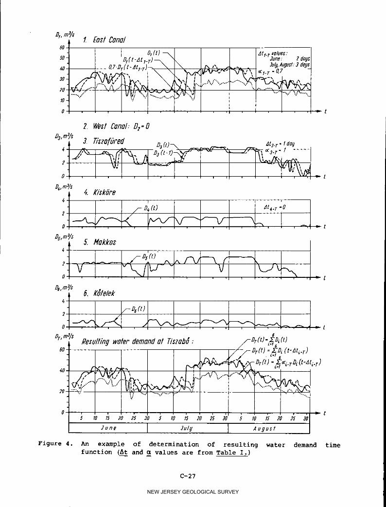
DI,restsI EastCanal
6O
01(t)_ zltFr values."50- D,(t-z]t.,_T) _ "\ June: Zdo#s;Wy,_uyusI.";days40 O'7'Dl(t-Atl-r)_x \\ IN rN ..
,, __"_...,. t\ ,_,,,...,,,...,....._-_,.,,,':"-..¢....'%r_,_'_._ _N "i_-,_'- ""-eo 5 ..... • " V_J"_'-'."""_ _ _..-"V"..vi .........' "
.... .%j. ... "-,:10. ,..[:: "v "".. ,.'.....," "; ": ",1
0 ' , , , , "w"t
Z WestCanal:02=06,m_Is
4._ 3. 1-/szafOred aa0)_ _tj-r" Iday
...... ,u:),,__ _=._c- \ i ,,
O. , , "_'t
G m_/s
4 _ 4. /(iskbPe
- /- & (0 _t4.T-o2.
0. , , _ t
6Yls
4._ 5. HokkosII i
eV "L,,j AI-_ \ "O' , ,; "_t
&mS/*
4-! 5. Kdtelek- /-D8(t)
.--_ _ .,-_.-._.___O" • /"-_/-_'_ , "_ _'_
E
Dr'mJIs Pesultin#waterdemandat T/szab_: /-ar(O-_._,&O)
";" "t' k.""i" .,e ...
20 '. .,"".-%.
June July A uyust
_igure 4. An example of determination of resultlng water demand time£unction (At: and __ values are from Table I.)
C-27
NEW JERSEY GEOLOGICAL SURVEY
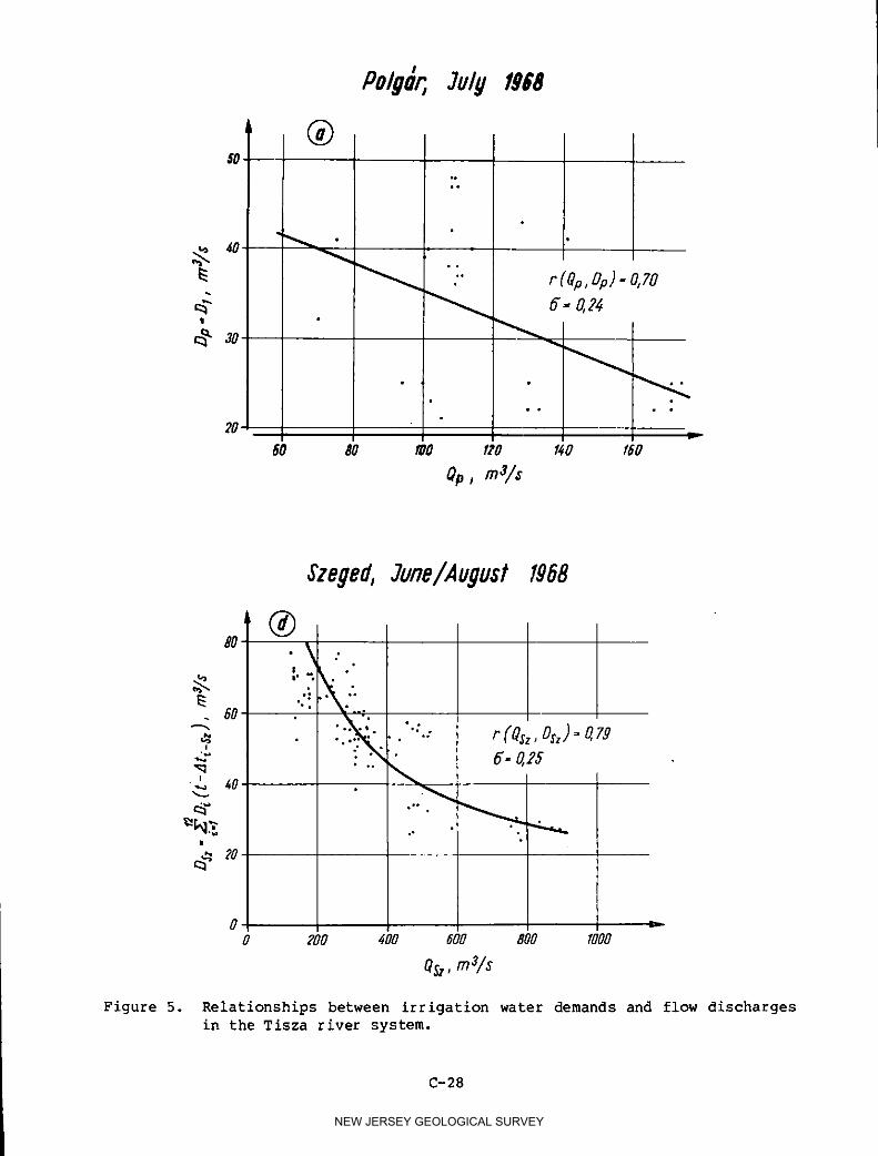
0
I_ _ ":" r(Qp,Dp)-O,70
_30
60 80 t00 f20 140 160
Op , m3/_
Sze#ed,3une/A@ust 1958
®80' _ ;
:'" "_
_ 60 ....
_" "'" "' "':.: r (OSz, OS,) = _79
._ _. 6.0,25.,_" 4o
,_._ ....I
0eoo 400 eoo aoo tooo
Figure 5. Relationships between irrigation water demands and flow dischargesin the Tisza river system•
C-28
NEW JERSEY GEOLOGICAL SURVEY

T#zob_,3u@1968
®7O
_-_ o
_, 60 ;
r(Or,Dr)"0,85I
_
60 80 I00 120 140 160
OT, rn3/s
_zeged,3ul_1964-60
"_':'_",,;...• . . c=o,2s
60 .:
-_ "':'" r( Os,,os_)- 0,82
-._.'... .'......
]
"_ " " _- I B,o._2 " " J
I ,: •
•_ 20 ",
500 I000 1500 2000 2500
Cls_, m%
Figure 5--Continued.
C-29
NEW JERSEY GEOLOGICAL SURVEY

Szeged,3uly IgG8
®gO
80
-_ • r (QSz,Osz)" 0,85
•'_ ._. g. o.og
_k12
.deo
150 200 250 300 350
QSZ, m3/_
Szeged,3une/Augus/ 1#54-69
;,°
• o,_,,,,. ,,°
"-_ ..;..:-'...:,.'......... . r(O,Sz,DSz)'O,,28
_._ "._.!:....:..: .. 6"0,33_, 40 ..-._'...
"'_'..._ :;...'...".._- """_.'!!....'..'.:.'.:;.'".'.i
'_" 0
_,_ ,........._ .• • _ °." ** °• • • ,o • . JJ
• ° ° °: '
g2o , . _ .
° •
500 1000 1500 2000 2500
Os,, m3/s
Figure 5--Continued.
C-30
NEW JERSEY GEOLOGICAL SURVEY
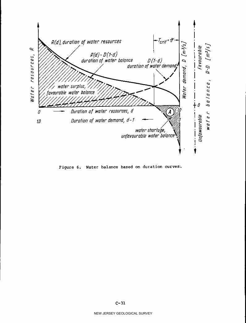
R(d),durationorwaterresources --7-crit=_"- _ _._
dJ Jdurationo[ water be D(1- _ _
_- durat/onof waterdemond/_
t...
_. water surplusj t _._ waterbalance _._ _
0 " Durationof water resources,d
Y,O Durationo/water demand,d-Z _ _ __
unfavourablewater
t
Figure 6. Water balance based on duration curves".
C-31
NEW JERSEY GEOLOGICAL SURVEY
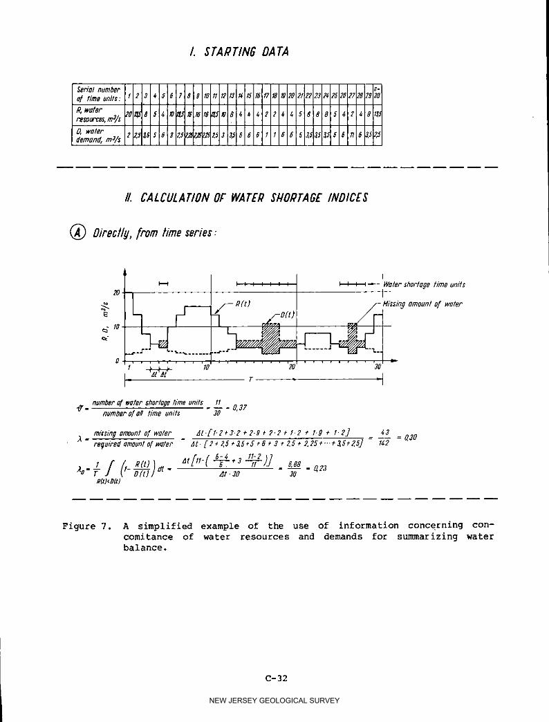
I. ;TAI?TIN6 DATA
t Serinl number s
o[ time units:
remurces,_/s
IL CALCULATIONOF WATERSHORTAGEINDICES
O/recite,Item timeseries:
I: : ', : : : : I I I I_ Woter 5ho/'te_8 t/_778units
D(t)
.__,..TT-:--:-?T,..._ ........." .
_,. numbero[ water shortogetime units = 11_. 0,37numberof e# time units 30
A= m/_slnQomounte[wMer_ _t-[t.2+3-2 �2.#�2.2_ l.2 �l.#+ t.2] 43 O.2Ore_eipBdemounto[wote/_ L1t.[2 3,5+S_5*$t2,5+2,25+..- ,5_1_2
F, / tt-2 }7i r i Rctj_ _tl't-c654-_ t, ,_ _,#8##}<DR)
Figure 7. A simplified example of the use of information concerning con-
comitance of water resources and demands for su_arizing water
balance.
C-32
NEW JERSEY GEOLOGICAL SURVEY

(_ Fromjoin/[requenc# [unction:
#, woler re£ources, m3/_0 fo 15 20
_ % %\ oe ,e _- _ffhoC_,y)_dy-_(3,a),.o,31
% 3 x._#
\ ho(x,#)dxdq_ I0 oo
°3 = (11-2).3+(6-_)._ = 43 =o'aoI'[.3 Œ���V�~�f'3"5_6"3_5���¢�f�_'2142
#
(_ Wi/#/he helpo[ durotioncurves:
_T_it-Q_-
D(l-d) _'= r_#-o,37_o- J I
.. _.___ _. , (_) . 1,4_-o,3oo- d _n(_-d)ad _,_2o,5 _._.j, ..o
D(l-d)-P(d)
Figure 7--Continued.
C-33
NEW JERSEY GEOLOGICAL SURVEY
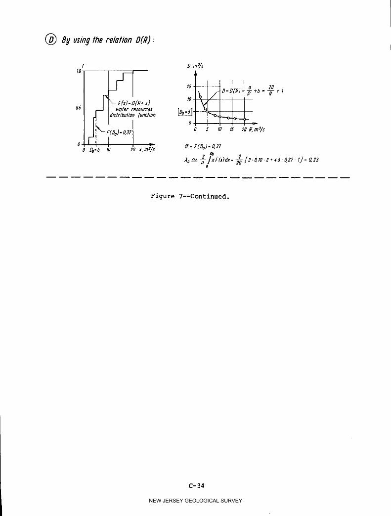
B# usingthe re/o/ionD(#):
F &m3/s
15- D-D(P) = _ $�=20
m"_) 1o / 7- * 1a5 rJ I water resources
Id,.tr,_utio.ru.ct/on _
(#o).o,3z 5 zo 15 2o#,,m31_
ori ] -o L_-_ 1o 2o x,m_/s _"[(#°)'0"37
2_o _._-2 /x F (_)dx- _ [ 3 . 0,f0. 2 �_,5.0,37 . lJ-0,23
o
Figure 7--Continued.
C-34
NEW JERSEY GEOLOGICAL SURVEY

38
g
__// I 57_: ho(x, u) dx dg -- T ZZ_,(,= Ig6 = 0,306yzx _ZYk
I ,_,_ajk(yk_Xj) 1 Y37
2 = x_l = - = O,233
// L s18oI _oo I Z'Z'aj,_IkT -'uh°(x'g')dx'dg -_-,j kO0
Figure 8. An example of the calculation of water shortage index in the case
of stochastic relationship between water resources and demand.
C-35
NEW JERSEY GEOLOGICAL SURVEY

A PHYSICAL APPROACH TO HYDROLOGIC PROBLEMS
by
J. R. PHILIP, B.C.E., D.Sc., F.A.A., F.R.S.
Chief, CSIRO Division of Environmental Mechanics, P.O. Box 821
Canberra City, A.C.T. 2601, Australia
D-I
NEW JERSEY GEOLOGICAL SURVEY

INTRODUCTION
My aim in this talk is to review for you the body of work relevant to
hydrology which has been carried out in our laboratory. This work covers a
time-span of 23 years. The present team includes about ten scientists, and
the average complement over the 23-year period has been, perhaps, six or
seven. During this time we have published well over 300 papers,* of which at
least 200 have implications for hydrology. Obviously I can do no more here
than attempt to convey something of the philosophy and the flavor of the
work, and to identify in a broad way those lines which seem to me to have
been the most important ones.
I must, at the outset, emphasize that our laboratory was not set up to
work specifically on hydrology. We began in 1952 as the Agricultural Physics
Section of the CSIRO Division of Plant Industry. (CSIRO stands for
Commonwealth Scientific and Industrial Research Organization, and is the
Australian Government institution for scientific research: the closest thing
to it in North America is--or, at least, was--the National Research Council
of Canada.) Consistent with the general philosophy of research administra-
tion in CSIRO, the terms of reference of our Agricultural Physics Section
were quite broad: the application of mathematical and physical approaches
and techniques to research problems in agriculture and plant biology. I am
convinced that the fruitfulness of our work has depended quite centrally on
the freedom we have had within CSIRO.
In the event, much of our early work dealt with problems arising in the
context of irrigated agriculture--and this led us straightway into studies of
water: water in the soil, water in plants, and water in the lower atmos-
phere. This early bias has persisted, so that we have contributed pretty
well continuously over the years to studies of the movement of water (and
other entities) through the soil, through vegetation, and through the lower
atmosphere.
In 1971 there were some organizational changes, and our laboratory became
an independent Division of CSIRO, the Division of Environmental Mechanics.
The range of our concerns has thereby been formally extended from agriculture
and plant biology to problems in the (more or less) natural environment as awhole. In fact, the content and character of our work has not really changed
very much, since we had, in any case, been working essentially on the physics
of transport processes in the natural environment.
WATER MOVEMENT IN UNSATURATED SOIL
The first broad area of our work which I shall discuss is that of water
movement in unsaturated soil.
In its natural state the soil is normally unsaturated: that is, it con-
tains both water and air. Most of the water involved in the hydrologic cycle
is located in unsaturated soil between the time of its arrival as rain at the
*The latest publication list (Anonymous, 1975) includes 328 papers and
two books. Copies of the publication list and reprints of many of the papers
are available on request.
D-2
NEW JERSEY GEOLOGICAL SURVEY

soil surface and that of its return to the atmosphere. A small fraction of
the precipitation does not enter the soil, but moves overland directly into
streams or lakes; and a second small fraction percolates downward through the
unsaturated 'zone of aeration' and joins the groundwater, i.e. the water in
the deep, habitually-saturated strata of soil, alluvia, or rocks. In a dry
country such as Australia, as much as 93% of the precipitation enters the
soil; and, of this, 92% returns directly to the atmosphere, only about 1%reaching the groundwater (Nimmo, 1949; Philip, 1954).
The processes of water movement in unsaturated soil thus play a central
part in the scientific study of the terrestrial sector of the hydrologic
cycle and in the related problems of irrigated and dry,land agriculture, of
plant ecology, and of the biology of soil flora and fauna. They are, in
addition, of great significance in connection with the transport through the
soil of materials in solution, such as natural salts, fertilizers, and urban
and industrial wastes and pollutants. Scientific phenomena of great interest
and importance include infiltration (the entry into the soil of water made
available at its surface); drainage and retention of water in the soil
strata; extraction of soil water by plant roots; and evaporation of waterfrom the soil.
Some of these hydrologic processes, of course, do not involve the soil
alone. It will be noted, for example, that the soil, the plant, and the
atmosphere form a thermodynamic continuum for water transport, so that the
proper study of natural evaporation from the earth's surface involves not
only soil physics, but also micrometeorology and, in the case of vegetated
surfaces, plant physiology. I shall say something about the soil-plant-
atmosphere continuum at a later point.
My immediate theme, however, is the mathematical-physical analysis of
water movement in unsaturated soil which has been developed in the last
twenty years or so. Until the late 1950's the various phenomena of water
movement in unsaturated soil tended to be studied separately and empirically
and, it must be said, rather inconclusively. Since then, however, applica-
tion of what is essentially the methodology of classical mathematical physics
has made possible a unified approach: the study of water movement in unsatu-
rated soils is now a reasonably coherent quantitative branch of physicalscience.
There are two basic ingredients in the now, more-or-less classical,
analysis which has emerged.
i. Recognition that the conservative forces governing the equilibrium
and movement of soil-water may be treated in terms of their associated scalar
potentials. We then have, in appropriate units,
= _(8) - z (i)
Here _ is the total potential and W, the moisture potential, is the potential
of the forces arising from local interactions between soil and water: capil-
larity, adsorption, and electrical double layers may be involved. We do not
need to know or to specify these forces in detail. It suffices that the
relation between _ and 8, the volumetric moisture content, can be measured by
well-established soil-physical techniques--so that _ (e) is essentially an
D-3
NEW JERSEY GEOLOGICAL SURVEY

experimentally determinable functional characteristic of any particular soil.z, the gravitational potential, is simply the vertical ordinate, taken posi-tive downward.
2. Recognition that Darcy's law holds for flow in unsaturated soils in a
generalized form in which the permeability (hydraulic conductivity) is afunction of e :
v = - K(e)V_ , (2)
where v is the vector flow velocity, and K is the hydraulic conductivity.
K(@) is then a second experimentally determinable functional characteristic
of the soil; and, as we shall see, the two functions _(e) and K(e) constitute
a necessary and sufficient characterization of the soil for the purpose of
analyzing unsaturated flow phenomena. Typical w(e) and K(e) functions are
shown in Figures 1 and 2.
Combining (i) and (2) and taking the divergence, we obtain the general
partial differential equation describing water movement in unsaturated soil:
De = v. (DYe) - dK . De . (3)St de 8z
Here the moisture diffusivity D = Kd_/de is a strongly varying function of e ;t denotes time. Figure 3 shows the D(e) relation for the soil for which ¥ (e)
and K(e) are given in Figures 1 and 2. It will be seen that D(e) varies
through some four decades over the e-range. The second coefficient in equa-tion (3), dK/de, varies over several more. This very strong nonlinearity is
typical.
It will be understood that the various phenomena mentioned earlier, such
as infiltration, correspond to solutions of equation (3) subject to the
appropriate initial and boundary conditions; so that (3) enables the integra-
tion of a seemingly disparate set of phenomena into one general theoretical
structure. This is, of course, unsurprising to physicists, but was something
of a novelty to soil scientists. Equation (3) is a nonlinear Fokker-Planck
equation. The nonlinearity is very strong and cannot be ignored, so thatprogress with this work has depended quite centrally on the development of
methods of solving (3) in all its nonlinearity. We note in passing that in
horizontal systems and in other cases where gravity may be neglected, (3)reduces to
8e = v. (DYe), (4)
8t
so that we are also concerned with the nonlinear diffusion equation (4).
We have been able to establish a fair body of solutions of (3) and (4)
(e.g., Philip, 1969; 1974); and these describe the experimental data fairly
well (e.g., Philip, 1957; 1969).
Figure 4 shows a typical solution of the flow equation (3) corresponding
to the process of infiltration into our illustrative soil with uniform ini-
tial moisture content 8o 0.2376. The saturation moisture content e10.4950. It will be noted that the early stages are characterized by
D-4
NEW JERSEY GEOLOGICAL SURVEY

similarity behaviour, with the length scale of the wetting profile propor-
tional to t_ . There is then a gradual transition until, for large t, a
wetting front of essentially constant shape advances into the soil at con-
stant velocity.
The present brief account necessarily passes over many complications and
generalizations of this field of work: these include capillary hysteresis,
the effects of entrapped air, water transport in the vapor phase, and temper-
ature effects. Extensions to the work which are being actively pursued in
our laboratory at present include the generalization to soils subject to vol-
ume change (e.g. Philip, 1973) and study of the hydrodynamic stability of
flows in unsaturated soil (Philip, 1975a,b).
TRANSPORT OF WATER AND ENERGY IN THE LOWER ATMOSPHERE
Let me now say a little about our work on the transport of water and
energy in the lower atmosphere.
The evaporation of water involves not only processes of transport of
liquid water to, and of water vapor from, the evaporation site, but also the
supply of energy (latent heat) needed for the phase change. A proper con-
sideration of water transfer in the lower atmosphere therefore requires that
we take cognizance not only of the transfer processes for water, but also for
energy.
We have, in this connection, done a fair amount of work on the turbulent
transport of water vapor and of heat in the lower atmosphere. When condi-
tions are believed to be essentially constant in the horizontal, the problem
may be taken to be one-dimensional and is relatively straight-forward, at
least in the airlayers above any vegetation.
In the real world, however, conditions do not stay conveniently uniform
in the horizontal. Some of the most obvious non-uniformities are due to
man's intervention in the hydrological cycle, such as the development of an
irrigation area, or the storage of water in a reservoir, in an arid region.
In such circumstances we desire to know the answers to questions such as how
evaporation (or evapotranspiration) and the microclimate vary as we move
downwind of a change in surface conditions.
We have studied these questions both theoretically and experimentally.
The theory is based on setting up simultaneous equations for the turbulent
diffusion of water vapor and heat in the lower atmosphere and solving them
subject to appropriate boundary conditions, including the energy balance at
the ground surface. We have found that theory is at least adequate to pre-
dict the order of magnitude of the observed effects (Philip, 1959; Rider,
Philip, and Bradley, 1963).
There are other problems connected with the transport of water vapor and
other entities in the lowest part of the atmosphere: one is that of trans-
port in the air layers within vegetation. In such regions the air flows and
the patterns of turbulence are very complicated and all the surfaces of vege-
tation act quite differently as sources (or sinks) of the various entities of
interest, such as momentum, sensible heat, and water vapor. Some progress
has, however, been made with untangling these matters (e.g. Denmead, 1964;
D-5
NEW JERSEY GEOLOGICAL SURVEY

Philip, 1964) so that progress is being made with the processes of
vegetation-atmosphere interactions.
WATER TRANSPORT IN THE SOIL-PLANT-ATMOSPHERE CONTINUUM
Finally, a word about the matter of the whole continuum of the soil, veg-
etation, and the lower atmosphere as a vehicle for the transport of water.
The system is clearly very complicated, and it might seem to be a hopeless
undertaking to attempt to analyse the process in any detail.
Fortunately, thermodynamics provides a basis for treating the processes
in these various regions in a unified way.
The energy state of water in the soil, the plant, and the atmosphere are
all expressible in terms of a thermodynamic potential (in fact the partial
volumetric Gibbs free energy) and it can be shown that water moves in all
parts of the complicated soil-plant-atmosphere system down the gradient of
this potential (Philip 1957d, 1966).
Water is taken up by the plant roots, and is transferred through the root
tissues to the conducting vessels of the plant, and in these vessels to the
mesophyll tissues of the leaves; it moves through these tissues to the evapo-
ration sites, which are primarily the walls of the substomatal cavities. The
final transfer of water from the substomatal cavities through the stomata of
the leaves is a process of molecular diffusion of water vapor.
Schematically (Figure 5) one can look on the passage of water through the
system as a flow through a sequence of resistances in series down a gradient
of #. This concept gives a useful first picture, but it must be emphasized
that for real plants the three-dimensional disposition of roots, leaves, and
other plant parts makes for a more complicated hydraulic problem.
There is a whole body of work going on, involving soil physicists, micro-
meteorologists, and plant physiologists, devoted to improving methods of
measuring the energy state of water in various parts of the soil-plant-
atmosphere continuum and to measuring the rates of transfer of water through
various parts of the system. Models of the soil-plant-atmosphere are becom-
ing, in consequence, more accurate, more convincing and, one hopes, more use-ful.
REFERENCES
Anonymous (1975). Publications, Environmental Mechanics, CSIRO.
Denmead, O. T. (1964). Evaporation sources and apparent diffusivities in a
forest canopy. J. Appl. Meteorol. 3, 383-389.
Moore, R. E. (1939). Water conduction from shallow water tables. Hil@ardia
12, 383-401.
Nimmo, W. H. R. (1949). The world's water supply and Australia's portion of
it. J. Inst. En@. Aust. 21, 29-34.
D-6
NEW JERSEY GEOLOGICAL SURVEY
Philip, J.R. (1954). Some recent advances in hydrologic physics. J. Inst.
En 9. Aust. 26, 255-259.
Philip, J. R. (1955). The concept of diffusion applied to soil water. Proc.
Nat. Acad. Sci. India, Sect. A 24, 93-104.
Philip, J.R. (1957a). The theory of infiltration: i. The infiltration
equation and its solution. Soil Sci. 83, 345-357.
Philip, J.R. (1957b). The theory of infiltration: 2. The profile atinfinity. Soil Sci. 83, 435-448.
Philip, J. R. (1957_). The theory of infiltration: 3. Moisture profiles and
relation to experiment. Soil Sci. 84, 163-178.
Philip, J. R. (1957d). The physical principles of soil water movement during
irrigation cycle. Proc. Contr. Int. Comm. Irri_. Drain. 3rd (SanFrancisco, 1957). pp. 8.125-154.
Philip, J.R. (1959). The theory of local advection: i. J. Meteorol. 16,535-547.
Philip, J. R. (1964). Sources and transfer processes in the air layers occu-
pied by vegetation. J. Appl. Meteorol. _, 390-395.
Philip, J.R. (1966). Plant water relations: some physical aspects. Annu.
Rev. Plant Physiol. 17, 245-268.
Philip, J.R. (1969). Theory of infiltration. Adv. H_drosci. 5, 215-296.
Philip, J.R. (1973). Flow in porous media. In 'Theoretical and Applied
Mechanics'. (Eds. E. Becket and G. K. Mikhailov.) Proc. 13th Int.
Congr. Theor. and Appl. Mech., Moscow, 1972, pp. 279-294.
(Springer-Verlag: Berlin.)
Philip, J. R. (1974). Recent progress in the solution of nonlinear diffusion
equations. Soil Sci. 117, 257-264.
Philip, J.R. (1975a). Stability analysis of infiltration. Soil Sci. Soc.
Amer. Proc. (in press).
Philip, J.R. (1975b). The growth of disturbances in unstable infiltration
flows. Soil Sci. Soc. Amer. Proc. (in press).
Rider, N. E., Philip, J. R., and Bradley, E. F. (1963). The horizontal trans-
port of heat and moisture--a micrometeorological study. Q.J.R. Meteorol.Soc. 89, 507-531.
D-7
NEW JERSEY GEOLOGICAL SURVEY

-10 5
_104
-103
_102
(m) -10
-1
_10-1
_10-2 I I0 0-1 0.2 0'3 0.4 0"5
6
Figure I. Dependence of moisture potential, _ , on moisture content, e , for
Yolo light clay (Moore, 1939).
D-8
NEW JERSEY GEOLOGICAL SURVEY

12 o
10
8
108 K(m sec-1) 6
/0
/0
0 o C_0_'0°0I I I i I
0"1 0.2 0"3 0.4 0.5
9
Figure 2. Dependence of hydraulic conductivity, K, on moisture content, 8 ,for Yolo light clay (Moore, 1939).
D-9
NEW JERSEY GEOLOGICAL SURVEY
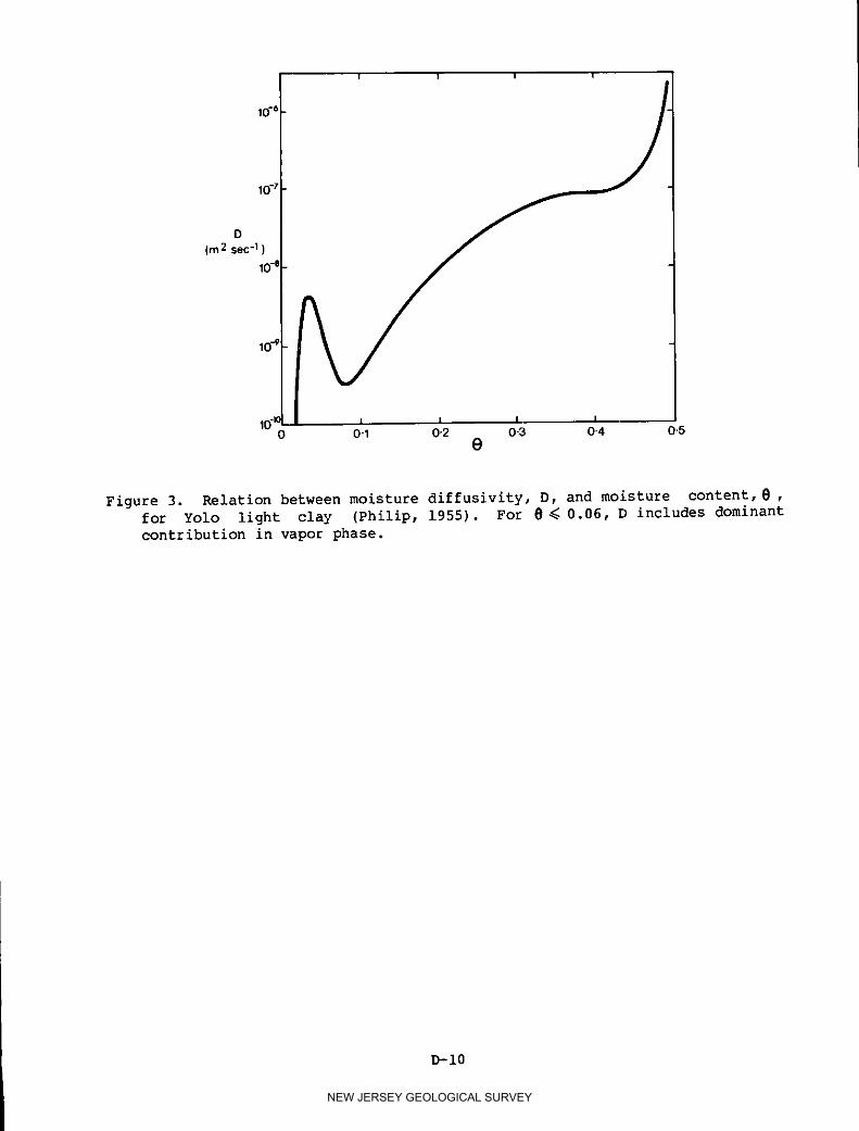
I I I I
10-7
D
(m 2 sec-1)
I I i I0 0"1 0"2 0"3 0"4 0.5
8
Figure 3. Relation between moisture diffusivity, D, and moisture content, e ,
for Yolo light clay (Philip, 1955). For @ _ 0.06, D includes dominant
contribution in vapor phase.
D-10
NEW JERSEY GEOLOGICAL SURVEY

O0° e o_104 I I
O2
2x10 5
0-4
0"6
z 0"8(m)
1.01.5x106
1.2
2x10 6
'1-4
1.6 I 1 ! I
Figure 4. Computed moisture profiles for one-dimensional infiltration in Yolo
light clay (Philip, 1954; 1957a,b). Numerals on each profile represent
value of t (sec) at which profile is realized.
D-II
NEW JERSEY GEOLOGICAL SURVEY

-12000
-I0000 I!
-8000
-6000
-4000
-2000
® .1 8._z(m) -
-400
3-300
-200 2
-100
1
0A B C D E F GH J K L).Soi:-I= Root _-:= Stem _I-_ Leaf ---_--Atmosphore_,_
Figure 5. The soil-plant-atmosphere continuum showing profiles of total
potential 4: (i) during normal transpiration; (2) during temporary wilt-
ing; (3) at permanent wilting. Points of the transpiration path: A,soil (a definite distance from plant root); B, surface of root hairs and
of absorbing epidermal cells; C, cortex; D, endodermis; DE, vessels and
tracheids in xylem; E, leaf veins; F, mesophyll cells; FG, intercellular
space and substomatal cavity; GH, stomatal pore; HJ, laminar sublayer if
present; JK, turbulent boundary layer; KL, free atmosphere; DPD w
denotes #-value at incipient plasmolysis of root cells (after Philip,
1957d).
D-12
NEW JERSEY GEOLOGICAL SURVEY
FACTOR ANALYSIS OF WATER QUALITY DATA IN NEW JERSEY:
EVALUATION OF ALTERNATIVE ROTATIONS
by
Dr. ROBER_ NORDON
Dept. of Geography
Rutgers University
New Brunswick, N. J.
E-I
NEW JERSEY GEOLOGICAL SURVEY

ABSTRACT
A set of water quality data from the Passaic River Basin in New Jersey
was factor analyzed. The data consisted of thirteen variables collected at
semi-monthly to monthly intervals over a twenty-year period (1950-69). Using
an eigenvalue cutoff of unity, varimax rotation resulted in three character-
istic factors: i) a flow-chemical factor (high loadings on discharge, pH,
alkalinity, and chlorides); 2) an oxygen factor (high loadings on DO, satura-
tion, and occasionally temperature); and 3) an appearance factor based on
color and turbidity. To see if alternative rotations would affect factor
structure, the same sets of data were factor analyzed using another type of
orthogonal rotation (quartimax) and four types of oblique rotation (covari-
min, biquartimin, quartimin, and direct quartimin). The results indicate
that alternative rotations had only a minimal effect on factor structure out-
put. The low to moderate factor correlation coefficients on most of the
oblique rotations suggest that the initial choice of the varimax orthogonalsolution was reasonable.
INTRODUCTION
Factor analysis is one form of multivariate analysis wherein a set of
intercorrelated variables are collapsed to form a smaller number of composite
variables, or factors (13, 17). These factors may then be rotated to yield a
set of independent, uncorrelated factors. Thus, factor analysis may assist
in the interpretation of variable relationships.
Although the application of factor analysis to problems in the social and
behavioral sciences is far more extensive than in the field of hydrology, a
fair-sized literature exists. For example, Wallis (19) used factor analysis
in a study of the agents that contribute to soil erosion and stream sedimen-
tation in northern California. Dawdy and Feth (4) applied factor analysis to
results of chemical analyses of ground water samples from the Mohave River
Valley in California. Matalas and Reiher (15) felt that factor analysis was
technically underdeveloped, a view seconded by Wallis (20) who also felt,
however, that the technique was a powerful tool for screening variables.
Rice (16) suggested varimax rotation as an aid in rationally interpreting
factors resulting from a study of hydrologic relationships. Eiselstein (7)
used a principal component regression analysis with varimax rotation of the
factor weight matrix as a means of synthesizing flow records for small
ungaged watersheds. Annual precipitation and runoff data from fourteen
watersheds in Ohio and seven watersheds in Texas were subjected to principal
component and factor analysis by Diaz, Sewell, and Shelton (5) in an attempt
to identify the factors affecting the water yield of the basins. Knisel (14)
used factor analysis on thirteen variables for five reservoirs in Texas to
determine which variables were significant for estimating reservoir losses on
the fissured limestone terrain. Morphometric data consisting of five param-
eters from five landscapes in eastern Australia were factor analyzed by
Abrahams (i) in an attempt to associate departures from topological random-
ness with the evolutionary decline of relief. Jackson (12) used factor anal-
ysis to study the relationship between variations in shoreline physiography
and water level fluctuation as perceived by reservoir recreation users.
E-2
NEW JERSEY GEOLOGICAL SURVEY

The first purpose of this paper is to examine the temporal changes in
water quality in the Passaic River Basin in New Jersey during 1950-69, using
factor analysis as a tool to extract the major sets of information from the
data. The period in question included a major period of suburbanization and,
in turn, a major impact on watershed quality, and periodic events such as the
record drought of 1962-66. It was hoped that the relative effects of these
trends and events could be isolated by factor analysis.
A second purpose is to test the impact of alternative factor analytic
rotations on the information that is extracted from the raw data. The goal
is to see the effect of varying rotations on the factor structure output.
METHODOLOGY
The factor analyses discussed in this paper were calculated with a number
of conservative assumptions regarding the degree of information covariance.
First, the communality was estimated by using the square of the multiple cor-
relation coefficient (R2) between each variable and all other variables in
the data set. These communalities would appear along the principal diagonal
of the correlation matrix. Alternative estimates of the communality could
have been chosen; for example, ones could be inserted in the principal diago-nal. This procedure then assumes that all of the variance of each variable
is related to the common factors of the data set. The true communality pre-
sumably lies between the R2 and unity estimates; thus, the R 2 estimate isprobably more realistic.
The BMDO8M factor analysis program (6) extracts a set of factors by the
principal components method. In order to increase the interpretability of
the resulting factor loading patterns, the unrotated factor loadings are
rotated. The first rotation used was the varimax solution, which involves a
series of orthogonal transformations of factor pairs. The varimax orthogonalroutine is the most commonly used form of rotation.
Another type of orthogonal rotation is the quartimax solution. However,
it is less commonly used, inasmuch as it tends to load more variance on thefirst factor.l
The second conservative assumption followed was that rotations were to be
performed on factors only if the eigenvalues exceeded unity. In almost all
cases, this arbitrary rule ensured that all factors accounted for at least as
much as one of the original variables. In order to maintain uniformity among
factor structures on some data sets, a few analyses were repeated with astipulated number of factors to be rotated.
At this point, a methodological question arises: to what extent are we
producing an artifactual bias in our output by forcing the data to yield a
set of independent, uncorrelated factors? Perhaps data from the real world
are inextricably interrelated, especially as the size of the observation unit
decreases. Two recent studies by Hughes and Carey (10) and Greenberg and
iSee Rummel (Ref. 17, footnote i, pp. 390-91) for a fuller discussion ofthis point.
E-3
NEW JERSEY GEOLOGICAL SURVEY

Hughes (8) discuss the validity of the orthogonal model and the resulting
possibility of biased output.
To help resolve this matter, a variety of oblique rotations can be per-
formed. In addition to the usual output of factor loadings and scores,
oblique rotation yields a set of factor correlations which can indicate the
degree of departure from orthogonality and zero correlation. The oblique
rotations used in this study include the direct quartimin (utilizes a struc-
ture matrix), the quartimin (favors high factor correlations), the covarimin
(favors low factor correlations), and the biquartimin (compromises between
the biases of the quartimin and covarimin).
APPLICATION OF FACTOR ANALYSIS TO WATER QUALITY DATA
PASSAIC RIVER BASIN, NEW JERSEY
The data consist of thirteen water quality variables collected at semi-
monthly to monthly intervals over a twenty-year period from 1950 to 1969 (see
Table i). The sampling site on the main stem of the Passaic River in New
Jersey just above the confluence with the Pompton River is part of a network
of surveillance stations maintained by the Passaic River Water Cormnission at
its own expense. Previous investigation by Carey, et al (3) had indicated
that some of the best water quality information in New Jersey was routinely
collected by large water supply agencies.
The nearly 5,000 pieces of information were grouped into six time periods
(1950-53, 1954-56, 1957-59, 1960-63, 1964-66, and 1967-69) so as to maintain
a favorable ratio of cases to variables. 2 Fortunately, the groupings
tended to coincide with periods of above-normal, normal and below-normal pre-
cipitation totals for northern New Jersey as discussed by Anderson and Faust
(2). This situation is desirable, as precipitation obviously influences dis-
charge which is a very important variable in water quality studies. Thus, a
certain degree of homogeneity within each time period was imparted to the
study.ORTHOGONAL ROTATION
The conservative eigenvalue cutoff of unity resulted in three factors
being rotated for five of the six time periods; the remaining 1957-59 period
was rerun so as to yield three factors. Ranked in order of importance, the
three characteristic factors resulting from varimax rotation were as fol-
lows: i) a flow-chemical factor exemplified by high loadings on discharge,
pH, alkalinity, and chlorides; 2) an oxygen factor (high loadings on DO,
saturation, and occasionally temperature); and 3) an appearance factor based
on color and turbidity.
Somewhat similar results were obtained from the quartimax rotation, but
the structures were not as clear since the solution favors high loadings on
the first factor. In Table 2, which shows the rotated orthogonal factor
2A rough rule of thumb in factor analysis is that the ratio of the num-
ber of cases to variables should be at least 2:1. In this study, the ratio
ranged from 2.8:1 to 5.5:1.
E-4
NEW JERSEY GEOLOGICAL SURVEY

loadings for a sample time period, note how the first factor for the quarti-
max solution accounts for 41.6 percent of the total variance, as compared to
30.0 percent for the varimax solution. Also, although temperature in the
varimax solution is shown to have a high inverse loading with DO and satura-
tion, the relationship is not clear during the other time periods (Table 2).
In particular, the temperature-DO relationship broke down during the 1950's,
as indicated by the two variables not loading highly together in the same
factor. The relationship improved during the three time periods of the1960 's.
The cumulative percentage of total variance explained (which does not
change with the type of rotation) ranged from 57 percent in 1950-53 to 71
percent in 1967-69, averaging 65 percent for the two decades. Surprisingly,
the degree of explanation offered by the factor analytic model was quite sta-
ble during the study period, even rising during 1967-69. This stands in
sharp contrast to similar studies on the Raritan River in New Jersey, wherein
the explanation decreased noticeably during the 1960's (9).
The interbasin differences can be attributed to several factors. First,
the data set for the Raritan consisted of nine water quality variables as
compared to the thirteen available for the Passaic. Second, since the
Raritan data was collected (by the Elizabethtown Water Co., another large
water supply agency) at weekly intervals, the information could be grouped
into an annual series. Thus, the particular assemblage of variables and the
different groupings of time periods could explain part of the interbasin var-
iations in behavior. At any rate, the factor analytic model appears to
detect changes in instream interactions among the variables over time. Per-
haps the secular increase or decrease in the cumulative degree of explanation
can be attributed to perturbations of the steady state caused by land use
changes within the basin and varying effluent loading patterns. At this
point, it is unclear why the explanation should be increasing for the Passaic
basin while the Raritan basin experiences a decline, since both data sets are
internally consistent (i.e., the variables within each set are the same from
time period to time period).
OBLIQUE ROTATION
As previously mentioned, oblique rotation yields a set of correlation
coefficients among the factors. Different factor correlations are obtained
for each of the time periods for each of the four types of oblique rotations(Table 3). As expected, the factor correlations varied from the covarimin
set of low coefficients (averaging .08) to the quartimin set of high coeffi-
cients (averaging .40), with the biquartimin ranging in between (.13). The
direct quartimin coefficients (.15) were similar to those of the biquarti-
min. If we accept the last type of oblique rotation as a compromise solu-
tion, we can then conclude that most factor correlations are below .25; thus,
the orthogonal solution should not be very different from several of theoblique solutions.
This assumption of similar factor structures is borne Out by examiningthe output from the oblique rotations. Three characteristic factors emerge
from all rotations (flow-chemical, oxygen, and appearance), albeit with
slightly different factor loadings (Tables 4 and 5 show the output for a sam-
ple time period). The quartimin rotation presents special problems, inasmuch
E-5
NEW JERSEY GEOLOGICAL SURVEY

as the rotated factor loadings may exceed unity. Indeed, during 1964-66 when
factor correlations averaged .98 (see Table 3), several factor loadings on
the quartimin exceeded 5.0. Obviously, interpretation of the loadings under
these circumstances becomes quite difficult. Note that 1964-66 marked a
drought period of unprecedented severity.
DISCUSSION
The results of this study suggest that the use of alternative rotations
on the water quality data from a downstream station on the Passaic River does
not unduly affect factor structure interpretation. Perhaps this result is
not unexpected, inasmuch as factor correlations were generally moderate.
Thus, the assumption of orthogonality in the factor model is reasonable inthis instance.
Of all the rotations, the varimax orthogonal rotation is probably the
most desirable one to use for the following reasons:
i) The orthogonal solution yields a set of uncorrelated factor scores
which can be later used as independent variables in a multiple regression
problem.
2) Factor structures can be quantitatively compared by using a computer
program called RELATE as long as the data are rotated orthogonally. As dis-
cussed by Veldman (18), the program accepts as input the factor loading ma-
trices that were obtained from an orthogonal factor analysis of identical
sets of variables. The factor axes are then rotated until maximum overlap
between corresponding test vectors in the two structures is attained. The
degree of rotation required is expressed as the cosine of the angle between
the factor axes. These cosines may be interpreted as correlations between
the factor variables, thereby facilitating quantitative factor structure
comparisons.
3) The percent of total variance explained by each rotated factor is
available with orthogonal rotation, whereas only the sum of squares for each
factor can be provided with oblique rotation. Thus, the orthogonal solution
allows one to rank more accurately the rotated factors in terms of statisti-
cal explanation and importance.
Given the advantages of the varimax rotation, one would prefer not to use
the other types of rotation. However, the interpretation of the factor
structure output may be biased unless the extent of departure from orthogo-
nality is assessed. Therefore, the following procedures are recommended for
the analysis of new sets of data.
First, use the biquartimin rotation as a compromise between the high and
low factor correlation biases of the quartimin and covarimin to test for
covariance among the factors. The quartimin should be avoided because it may
yield factor loadings greatly exceeding unity. The output from this study
suggests that the direct quartimin should give results similar to those of
the biquartimin and is therefore redundant.
Second, if the factor correlations from the biquartimin or direct quarti-
min are .25 or less, the factors may be considered operationally independent
and the orthogonal solution may be used. In that case, it is preferable to
E-6
NEW JERSEY GEOLOGICAL SURVEY

use the varimax rotation, since the quartimax orthogonal solution loads most
of the variance on the first factor, an undesirable trait with respect to
clarity of interpretation.
The procedures described above appear to be in accord with the views of
Hunter (ii), who suggests that only method-independent factors be treated as
important substantive findings. A method-independent factor is defined as a
factor which has similar loading patterns in both the orthogonal and oblique
rotations.
CONCLUSIONS
A set of water quality data from the Passaic River Basin of New Jersey
was factor analyzed and then subjected to six different types of rotation.
The data set consisted of thirteen variables collected at semi-monthly to
monthly intervals from 1950 through 1969. The twenty years of record were
divided into six time periods of three to four years each.
Although there was some variation, the two types of orthogonal rotation
(varimax and quartimax) and the four types of oblique rotation (covarimin,
biquartimin, quartimin, and direct quartimin) yielded similar factor struc-
tures for each of the time periods. Using an eigenvalue cutoff of unity for
rotation, three characteristic factors emerged: i) a flow-chemical factor
(high loadings on discharge, pH, alkalinity, and chlorides); 2) an oxygen
factor (high loadings on DO, saturation, and occasionally temperature); and
3) appearance factor based on color and turbidity.
The output from the oblique rotations includes a set of factor correla-
tions which dimension the degree of factor independence. The covarimin and
quartimin rotations are biased towards low and high factor correlations,
respectively, whereas the biquartimin and direct quartimin represent compro-
mise solutions. The factor correlations for the biquartimin and direct
quartimin average .14 in this study. Thus, the assumption of orthogonality
in the factor analytic model is reasonable and the varimax orthogonal solu-
tion, which has many advantages, may be employed with greater confidence.
These findings are important because the orthogonality of the factors sup-
ports the contention that some water quality parameters may be modeled inde-
pendently of the effects of others, while other indicators of water quality
may be used as surrogates for a larger set of interdependent indicators.
REFERENCES
i. Abrahams, A. D., "Factor Analysis of Drainage Basin Properties: Evi-
dence for Stream Abstraction Accompanying the Degradation of Relief,"
Water Resources Research, 8 (1972), 624-33.
2. Anderson, P. W., and Faust, S. D., "Impact of Drought on Quality in a
New Jersey Water Supply System," Water Resources Bulletin, 8 (1972),750-60.
3. Carey, G. W., Zobler, L., Greenberg, M. R., and Hordon, R. M., Urbaniza-
tion, Water Pollution, and Public Policy, Rutgers University: Centerfor Urban Policy Research, 1972.
E-7
NEW JERSEY GEOLOGICAL SURVEY

4. Dawdy, D. R., and Feth, J. H., "Applications of Factor Analysis in Study
of Chemistry of Ground Water Quality," Water Resources Research, 3
(1967), 505-10.
5. Diaz, G., Sewell, J. I., and Shelton, C. H., "An Application of Princi-
pal Component Analysis and Factor Analysis in the Study of Water
Yields," Water Resources Research, 4 (1968), 299-306.
6. Dixon, W. J. (editor), Biomedical Computer Programs, University of
California: Publications in Automatic Computation, No. 3, (1970),90-103.
7. Eiselstein, L. M., "A Principal Component Analysis of Surface Runoff
Data From a New Zealand Alpine Watershed," Proceedings, International
Hydrology Symposium, Fort Collins, Colorado, Vol. i, (1967), 479-89.
8. Greenberg, M. R., and Hughes, J. W., "Analysis of Human Territoriality:
Alternative Factor Analytic Methodologies," New York Statistician, 25(1974), 3-7.
9. Hordon, R. M., "A Factor Analysis of Selected Water Quality Variables in
Central New Jersey During 1960-69," paper presented at the annual meet-
ing of the American Geophysical Union, Washington, D.C., April 1972.
i0. Hughes, J. W., and Carey, G. W., "Factorial Ecologies: Oblique and
Orthogonal Solutions. A Case Study of the New York SMSA," Environment
and Planning, 4 (1972), 147-62.
ii. Hunter, A. A., "Factorial Ecology: A Critique and Some Suggestions,"
Demography, 9 (1972), 107-17.
12. Jackson, R., "Factor Analysis of Shoreline Physiography and Perception
of Water Level Drawdown by Reservoir Shoreline Residents," Water
Resources Research, 9 (1972), 81-92.
13. King, L. J., Statistical Analysis in Geography, Englewood Cliffs, New
Jersey: Prentice Hall, 1969, 165-93.
14. Knisel, W. G., "A Factor Analysis of Reservoir Losses," Water Resources
Research, 6 (1970), 491-98.
15. Matalas, N. C., and Reiher, B. J., "Some Comments on the Use of Factor
Analysis," Water Resources Research, 3 (1967), 213-23.
16. Rice, R. M., "Multivariate Methods Useful in Hydrology," Proceedings,
International Hydrology Symposium, Fort Collins, Colorado, Vol. I,
(1967), 471-78.
17. Eummel, R. J., Applied Factor Analysis, Evanston, Illinois:
Northwestern University Press, 1967.
18. Veldman, D. J., Fortran Programming for the Behavioral Sciences, NewYork: Holt, Rinehart and Winston, 1967, 236-44.
E-8
NEW JERSEY GEOLOGICAL SURVEY

19. Wallis, J. R., "A Factor Analysis of Soil Erosion and Stream Sedimenta-tion in Northern California," Ph.D. thesis, University of California,
Berkeley, 1965.
20. Wallis, J. R., "Factor Analysis in Hydrology--An Agnostic View," Water
Resources Research, 4 (1968), 521-27.
E-9
NEW JERSEY GEOLOGICAL SURVEY

TABLE 1. PVWC - WATERQUALITY SAMPLING VARIABLES.a
I. Stream Discharge
2. Temperature, Water
3. Turbidity
4. Color
5. pH
6. Alkalinity
7. CO 2, Free
8. Chlorides
9. DO Dissolved Oxygen
10. Saturation, Percent
11. BOD - Biochemical Oxygen Demand
12. Bacteria Plate Count on Agar at 35.5 C
13. Coliforms - MPN/100 ml
a PVWC - PassaicValley Water Commission
E-IO
NEW JERSEY GEOLOGICAL SURVEY

TABLE2. ROTATED ORTHOGONAL FACTOR LOADINGS, 1967-69 a,b
Varlmax Quartlmax1 2 3 I 2 3
1. Discharge -64 43 13 (-76) 01 15
2. Temperature -01 (-86) 25 48 (-71) 24
3. Turbidity 04 24 (84) -08 23 (84)
4. Color -19 -18 (88) -04 -25 (88)
5. pH (88) -25 -01 (87) 29 -03
6. Alkalinity (81) -52 03 (96) 02 01
7. CO 2 60 -48 -07 (76) -06 -09
8. Chlorides (94) -15 -07 (86) 40 -10
9. DO -26 (95) 07 (-74) 64 08
10. Saturation -29 (87) 23 (-72) 56 24
1I. BOD (70) 33 03 40 66 02
12. Bacteria 35 -33 19 48 -08 18
13. Call forms 26 -27 29 37 -08 28
Percent TotalVariance 30.0 27.2 13.6 41.6 15.8 13.4
a Decimals omitted from all factor Ioadlngs. All Ioadlngsgreater than or equal to/0.70/ore indicated in parentheses.
b PVWC Station No. 1051.
E-II
NEW JERSEY GEOLOGICAL SURVEY

0 "_" 0 0", _0 0 U-) _0 0 0 0'. 0 _ 0". 0 09 0") 0
0 0 0 0 _ _ 0 "-- 0 0 _" 0 0 0 0 0
0C
r,. 0 --" 0 0 0 _ 0 _ 0 0 0• O0 O0 _0 O0 _0 _o
o 0 0 0 0 o0 0 0 0 0 0
_mo _o _o _-o _o -_o
??_ ?_ _oo_ Too_ ?oo_ ooo_
.E
_0 _0
z _ o o o o o oC _ o o o o o o
E
/
_O _O _O OO _O _O .9_0 _0 _0 _0 _0 _0
d 0 o o o o o o-- 0 0 0 0 0 0
E o
C _
[_ l-- II-- II-- II-- -- =E
_0 O0 _0 O0 _0
_- _ g g g g g
_ &'%l _ _ ¢'_1 (_9 _ (%1 _ "-" f%l (_ '-" _1 _ "(%1(")
0u<u. c,_ ,o o. _ ,o o,
I ! ! i | i
o _ _-.
E-12
NEW JERSEY GEOLOGICAL SURVEY

_ _ _ O QO0 Q_ Q_ _VVl II
N I_,0 _ _ 0 r_ _ o _o (>. o _ "0 (_" I_co l'Xl (o it) u3c_ o_ co (_1 c9 _i "_" i i i i l-o
-- -0('_ (_ 00_ cO (N O_ cO O- ,0,0",000("4(:0OO'',0 (N C9',0 CO CW
i I I _" _ I I _"
..0
Oo.,0I
__ O O ('Xl0 C,,I i)
°_ ° 0
- _,o.-o.o_,o_m_.-*_ o. :;._I I I _ _ I I _ ('3 0 ._
-- O
_ "-_ ,2"Oi _ _ _or_o ,n,_9.co _. o
I _ V , 0 0 0 _ 0 _ E _
'' - _o
• _ o_ __°_, _; _°°-=_1" I v I ! I I v -i-v
; o o.
- "E -o _ .o _ o0 Q;-O :- - -- 0 D
iF;
-_-o__o _E
E-13
NEW JERSEY GEOLOGICAL SURVEY

TABLE5. DIRECTQUARTIMIN ROTATED FACTOR LOADINGS, 1967-69a,b
1 2 3
1. Discharge -64 -30 13
2. Temperature 06 (86) 24
3. Turbidity 06 -30 (84)
4. Color -21 18 (87)
5. pH (90) 05 -01
6. Alkalinity (81) 34 02
7. CO 2 59 35 -08
8. Chlorides (96) -06 -08
9. DO -20 (-91) 08
10. Saturation -25 (-83) 24
11. BOD (75) -50 04
12. Bacteria 34 25 19
13. Collforms 25 20 28
Sumof Squares 4.05 3.06 I .74
a Decimalsomitted from all factor loadings. All Ioadlngsgreater thanor equal to/0.70/are indicated in parentheses.
b PVWC Station No. 1051.
E-14
NEW JERSEY GEOLOGICAL SURVEY

POLLUTION CRUNCH IN JAPAN
by
HUGH B. RIPMAN
Associate Columbia University Seminar onPollution and Water Resources
and Former Director of
Administration World Bank
F-I
NEW JERSEY GEOLOGICAL SURVEY

Ten years ago, no one worried much about pollution or the protection of
the environment in Japan. But public concern has grown steadily since that
time. This is evidenced by the fact that during one month in 1971, one
Japanese newspaper carried no less than 124 articles about various aspects of
the pollution problem. Some sensational incidents have attracted widespread
attention and anxiety. I will mention some of these incidents.
t>l.-wThe Minamata disease. This is a form of methyl mercury poisoning,
which was identified in 1956 in the coastal areas of Minamata Bay and in 1964
along the drainage basin of the Agano River. It is caused by the long-term
consumption of sea-foods with a high content of methyl mercury compounds. Its
symptoms include difficulties in walking and hearing, impairment of speech and
various sensory disturbances. More than 450 victims were found in the
Minamata Bay area, of whom 71 have died. In the Agano River basin more than
300 victims have been found, of whom 13 have died.
2. The Itai-itai disease. This is a form of cadmium poisoning, which
impairs the functioning of the kidneys and softens bone tissue. It was iden-
tified in the Jinzu River basin in Toyama prefecture, where wells and irriga-
tion water for rice paddies had been contaminated by effluents from a mine
belonging to a company of the Mitsui group. More than 120 victims have been
identified, of whom 42 have died. As the result of a suit brought against the
mining company, damages amounting to $450,000 have been awarded to 34 of the
victims. The surviving victims of this disease and of the Minamata disease
are receiving special benefits under the law concerning Special Measures forthe Relief of Pollution-related Patients.
3. Polychlorinated Biphenyls (PCB). In 1968 a number of people in dif- i
ferent parts of Japan suffered attacks of acute poisoning as the result of
eating a brand of rice bran oil. It was discovered that PCB (a chloride used
in heat conductors, condensers, carbonless copy paper and electrical insulat-
ing materials) had been used as a heating medium in manufacturing the rice
bran oil, and had leaked into the oil through a hole in a corroded pipe.
Since then PCBs have also been found in soil, in sea foods, in birds and in
human milk in Western Japan.
4. Pollution of the Seto Inland Sea. The so-called "Red Tide" -- due to
rapid proliferation of plankton which colours the water red -- was twenty
years ago a local phenomenon of limited importance in two small areas, only
sporadically occurring. The incidence of this phenomenon has grown steadily
over the years, and it now affects practically the whole of the Seto Inland
Sea, an area designated in 1934 as a national park, and widely known as a
treasure-house of marine resources. Not only has the scenic beauty of these
waters been marred, but as the result of the red tide the fishing industry has
suffered heavy losses. While scientists do not yet completely understand how
this phenomenon develops, the studies that have been made would seem to _how
that it is the result of the manifold pollutants which flow into the sea,
which include effluents from such industries as paper and pulp mills and vast
quantities of raw sewage. The Inland Sea has also been polluted by oil from
ocean-going ships. Finally, special problems are posed by the dumping of
plastic wastes, which not only affect fishing grounds, but also block up the
engine cooling water intakes of ships.
F-2
NEW JERSEY GEOLOGICAL SURVEY

5. Urban smog. This is the most obvious and most frequently experienced
kind of pollution for the largest number of people. Mount Fuji, which once
could be seen from Tokyo one day in every three, is now visible only one day
in seven. In 1971 nearly 50,000 people in and around the big cities of West-
ern Japan suffered eye, throat or lung irritation from photochemical smog.
Public attention was caught by an incident in July 1970 when 43 girls at a
high school playground in Tokyo suddenly became nauseated and fainted.
All these incidents and developments have been widely reported and aroused
much public concern and anxiety. Thousands of complaints and petitions have
been received from both urban and rural districts in all parts of the
country. The largest proportion of these complaints (over 33%) is concerned
with noise and vibration; offensive odors follow with nearly 24%; third comes
air pollution with about 18%. The total number of such complaints accepted by
regional public bodies in 1971 was more than 75,000.
An idea of the cost of pollution to the nation can be obtained from esti-
mates made for 1970. No attempt was made to quantify the costs of damage to
health, but the loss of production in agriculture and fisheries was estimated
at over 38 billion yen. Domestic expenses, such as additional laundry costs
and new paint, were estimated to be over 410 billion yen. Costs incurred by
industry for pollution prevention and control were 780 billion yen. (Large
scale industry has recently been spending about 10% of its total investment
funds on pollution control.) Government spending for protection of the envi-
ronment totaled over 300 billion yen. The total cost per citizen had risen
from 2,000 yen in 1960 to 4,500 yen in 1965 and 15,000 yen in 1970 - almost 8
times in i0 years.
Appropriations by ministries and agencies for pollution control and con-
servation of the natural environment rose from iii billion yen in 1971 to 169
billion yen in 1972 and 273 billion yen in 1973. Treasury investment and
loans relating to pollution control increased from 170 billion yen in 1971 to
263 billion yen in 1972 and 430 billion yen in 1973.
The foregoing paragraphs give a general idea of the magnitude of the pol-
lution problem in Japan, and of its serious effects on the citizen and the
economy. It may now be interesting to consider how the problem has arisen,and what has been done about it.
Japan's drive to modernize its economy dates from the beginning of the
Meiji era in 1868. Economic development has been rapid, and the pace of
development has accelerated very much since the end of the second world war.
As the result, Japan is today one of the leading industrial countries of the
world. However, investment in social capital has lagged behind. For example,
in 1965 only 15% of the population was served by sewer systems, and by 1971
the proportion had only risen to 22%. This compares with 90% in England(1963) and 71% in the U. S. A. (1968).
Moreover, the Japanese economy is so structured that it tends to produce
more pollution than the type of economic structure in other industrialized
countries. For instance, a French type of economic structure would generate.
about 40% less sulphur oxides, an American type 20% less and an English or
West German type 10% less. The same kind of pattern applies to BOD, particu-lates and industrial waste.
F-3
NEW JERSEY GEOLOGICAL SURVEY

The spectacular Japanese economic development .took place in a country
where population and industrial density have now almost reached an upper
limit. Annual production valued at $200 billion must be supported by only
10,000 km 2 of level land. Already twenty years ago gross national product
per equal area of level land was more than twice as much in Japan as in the
U. S. A. Today it is more than eleven times as much. The visitor to Japan is
struck by the fact that wherever he travels in the country, he is never out of
sight of the mountains -- but this reflects the fact that there is only 30
m2 of level land per person -- and this exiguous amount of level land
includes the roads, the railroads and the rice paddies. No wonder that ter-
raced fields ascend every little mountain valley and cover every side of many
hills. New steel plants and many other new industrial facilities have to be
constructed on land reclaimed from the sea.
The number of automobiles in use has increased dramatically. Between 1959
and 1969 the number of automobiles per 1,000 hectares of level land rose ten
times, from 130 to 1,300. This means that in 1969 the number of automobiles
per hectare of level land was no less than 8 times the corresponding figure
for the U. S. A. in that year, and that on the average in Japan more than oneautomobile was driven within each hectare of level land. It is clear, there-
fore, that air pollution from exhaust gas, noise and vibration have a much
greater impact in Japan than in other countries.
Pollution problems are aggravated because population and industry are con-centrated in a few areas. Two of these -- the so-called Pacific Belt and the
northern part of Kyushu -- cover only about one quarter of the land area, but
in 1964 they were responsible for 75% of the biochemical oxygen demand and for
nearly 70% of the total emission of sulphur oxides.
Pollution of rivers and streams flowing through urban areas is acute and
becoming worse rapidly, on account of the increase in untreated domestic sew-
age. The problem of garbage disposal is a serious one -- the total output of
garbage in 1970 was 35 million tons. Traffic congestion, with its accompany-
ing noise, vibration and air pollution is universal in all the crowded urbanand suburban areas.
Part of the pollution problem flows from the fact that industrial growth
has been concentrated in such industries as electric power, iron and steel,
paper and pulp, chemicals and ceramics. In 1970 these industries accounted
for over 80% of sulphur discharge. Paper and pulp, food industries, chemicals
and textiles were responsible for over 95% of the biochemical oxygen demand in
the same year.
Energy consumption per hectare of level land in 1969 was ten times that in
the U. S. A. World energy consumption just about doubled in the years from
1955 to 1970, while in the same period in Japan per capita energy consumption
increased more than 200% and absolute energy consumption 250%. Moreover, dur-
ing the last twenty years there has been a remarkable change in the sources
I fr_ which Japan obtains its energy. In 1955 thermal plants produced 25.7% of
all electricity. By 1970 the proportion had risen to 76.4% of a very much
larger total. Thermal plants burn mostly oil imported from the Near and Mid-
dle East, with a large sulphur content, which aggravates the air pollution
problem.
F-4
NEW JERSEY GEOLOGICAL SURVEY

Industrial water usage has also increased rapidly. In 1962 it accounted
for only 35% of total water usage; by 1969 it was already more than half total
usage. The three largest producers of biochemical oxygen demand load -- paper
and pulp, food industries and chemicals -- used 60% of total industrial
water. The paper and pulp industry has expanded at a particularly rapid rate
-- the Japanese people are almost 100% literate and voracious readers -- and
was responsible in 1970 for almost 50% of the biochemical oxygen demand load.
During the last twenty years, while total industrial production has grown
at a spectacular rate, the share of basic production goods has steadily
increased, and that of basic consumption goods has decreased. This partly
reflects the continuing and increasing investment in c_pital equipment and
construction and partly the need to increase exports to pay for imported raw
materials and fuel, which coincided with a very strong world demand for chemi-
cal products and for steel.
The economy has however grown so fast that even though the share of con-
sumption goods in total production has lagged behind that of production goods,
there has been a very large absolute increase in the production of consumption
goods, and especially in that of durable consumption goods. Parallel with
this goes an increasing problem in the disposal of discarded products of thiskind.
For instance, ownership of television sets skyrocketed in a few years. In
1958 only about 14% of the population owned a television set; five years later
the figure was over 90%. Less than 10% owned a refrigerator in 1958; ten
years later the figure was over 80%. Ownership of cars, air conditioners and
color television sets have all been rising rapidly. The use of disposable
packaging (non-returnable containers and plastic packaging) aggravates the
problem of solid waste disposal. Plastic waste disposal poses a special prob-
lem. Production shot up from about 10,000 tons in 1960 to 5 million tons in
1970. Plastic waste material was reported to be 1 to 3 million tons in 1970.
One result of these developments is that solid refuse collected in Tokyo has
been increasing about twice as fast as the population of the city.
Although the ownership of automobiles has risen rapidly -- from 1.5 mil-lion in 1955 to 19 million in 1970 -- the rise has been so recent that the
problem of disposal of junked automobiles is not yet serious, though it cer-
tainly will be in the future. The air pollution problem from automobile
exhaust, on the other hand, is already very serious. In Tokyo alone -- the
most recent figures available are for 1967 -- exhaust gases released 850,000
tons of carbon monoxide, 170,000 tons of hydrocarbons and 3,500 tons of nitro-
gen oxides into the air.
The various sensational incidents, the consequent public concern, the
ubiquitous evidence of pollution and the volume of complaints received have
all combined to make the protection of the environment an urgent political
issue. In consequence, many laws have been passed and many regulations
imposed to cope with the many different aspects of the problem.
A basic Law of Environmental Pollution Control was passed in 1967. This
law was strengthened in 1970. The budget for expenditures for environment
protection increased nearly five times from 1967 to 1972, and the figure for1973 is more than 50% above the 1972 level.
F-5
NEW JERSEY GEOLOGICAL SURVEY

Expenditure on research has grown rapidly and in 1972 the environmental
agency decided to coordinate the research activities of all other government
agencies in the field of environmental preservation, and to unify budget
expenditures for testing and research institutes belonging to other government
agencies, and for contracts with private organizations that are mainly devoted
to pollution control. In 1972 this unified budget for testing amounted to
2,300 million yen. In addition about 6,400 million yen was appropriated for
research and surveys by government agencies relating to pollutioncountermeasures.
It is interesting to compare these figures with the more than $300 million
spent in 1970 by the U. S. Government for pollution control research. How-
ever, Japanese industry -- especially paper and pulp, iron and steel, elec-
tricity and automobiles - stimulated by emission and effluent standard targets
established by government, is making a major effort to develop pollution con-
trol technology. The automobile industry, for instance, spent almost $100
million for this kind of research in 1972. But for industry as a whole,
expenditure for pollution control research and development is still less than
10% of total research expenditures.
An important step was taken by the government in 1971, when the Environ-
ment Agency was established and made responsible for laying down standards and
for coordinating action over the whole field of environment protection. The
following paragraphs give a general idea of the action taken to cope with the
most important threats to the environment.
Air Pollution
As of March 1973 environmental standards have been established with
respect to sulphur oxides, carbon monoxide and suspended particulate matter.
Similar standards for lead and nitrogen oxides are being considered. Air pol-
lution controls have been extended over the whole country. Emission standards
for soot and dust have been applied in 29 designated areas. Uniform emission
standards for the whole country have been fixed for cadmium, chlorine, hydro-
gen chloride, fluoride and silicon fluoride and lead. Emergency measures are
in force for special meteorological conditions.
Automobile exhaust standards have been established. The maximum permis-
sible amount of lead in gasoline has been laid down. Steps have been taken to
reduce the sulphur content of heavy oil and stack smoke.
A national Air Pollution Monitoring Network has been constructed with 15
stations. Some of these stations, in the Tokyo and Osaka areas, are linked by
telemetric information exchange systems. The 1973 budget included funds for
construction of an additional two stations.
Water Pollution
Environmental standards were established in 1970, covering over 500 dif-
ferent types of production, with penalties for violation of effluent stand-
ards. A special Water Pollution Control Law was passed in 1971. Strict
control has been established over effluents from mines and smelting plants.
F-6
NEW JERSEY GEOLOGICAL SURVEY

A new sewerage law became effective in 1971, and a third five year sewer-
age plan, beginning in that year, is designed to increase the proportion of
urban areas served by sewer systems from 22.8% (of 5,945 rm2) in 1970 to 38%
(of 8,490 rm2) in 1975. This would allow the proportion of urban populationserved to rise from 34.7% (of 62.8 million) in 1970 to 55% (of 75.4 million)
in 1975. This program will involve a total investment of 2,600 billion yen,
and in view of the urgency of the situation, expenditure is proceeding ahead
of the original schedule.
Dams are being built to reduce fluctuations in river flow, which otherwise
may be very marked in a country where rivers are relatively short and rapid.
A system of monitoring the condition of public waters is being installed.
A Marine Pollution Control Law was passed in 1970, which regulates the
drainage of oil and waste products from ships. Waste oil disposal facilities
are being constructed in port areas. High speed patrol boats and helicopters
are being used to maintain a system of marine surveillance.
Human Health
Areas in which the air is highly polluted have been designated as eligible
for aid under the 1969 law concerning Special Measures for the Relief of
Pollution-related Patients. By the end of March 1973 over 8,700 patients
affected by air pollution had been found eligible to receive financial aid to
meet their medical expenses. They were suffering from chronic bronchitis
(22.9%), bronchial asthma (34.8%), asthmic bronchitis (41%) and emphysema
(1.3%). Half of these patients were children under 9 years old; 20% were over60 years old.
Similar aid was being given to victims of the Minamata and Itai-itai dis-
eases and to victims of PCB poisoning.
Nature Conservation
Various areas of natural beauty, green belts on the border of urban areas,
etc. have been protected by making any proposed alteration to the state of
nature subject to special permission.
It is interesting to note that 13.5% of the total land surface of Japanconsists of publicly-owned parks. In these areas there is strict control of
trees and gravel mining.
These parks were visited by nearly 540 million people during 1971, an
increase of 60% over the 330 million visitors in 1966. Now public facilities
are being constructed to handle the garbage problem caused by the large number
of visitors, which seems likely to continue to grow.
Noise and Vibration
Standards were established in 1971 to cover noise and vibration caused by
factories, at construction sites, and by traffic on highways, super-express
trains and jet aircraft. Take-offs and landings of jet aircraft at Tokyo and
Osaka airports have been restricted within designated hours of the day.
F-7
NEW JERSEY GEOLOGICAL SURVEY

Offensive Odors
An Offensive Odor Control Law, which became effective in 1972, has given
prefectural governors the responsibility and authority to control the emission
by industry of substances causing offensive odors.
Polychlorinated Biphenyls
The manufacture of PCB's, the production of which had grown from 5,000
tons in 1968 to 11,000 tons in 1970, decreased from then on and completely
stopped in 1972. In September of that year practically all importation of
PCB's was forbidden. In August 1972 provisional permissible levels were laiddown for PCB content of human and animal food.
Agricultural Chemicals
An Agricultural Chemical Control Law was passed in 1970, resulting in a
complete ban on the use of DDT and similar compounds and the strict regulation
of the use of many other agricultural chemicals. Standards of Safe Use havebeen established.
Administration
The Environment Agency was established in 1971 to formulate the basic
principles for the conservation of the environment and to coordinate measures
taken by the various ministries and agencies active in the field. In that
year nine ministries and six agencies received appropriations for environmen-tal control and research.
The Environment Agency issues guidelines for pollution control programs,
and all proposed programs must be submitted to it for approval. It estab-lishes environmental and emission standards. It enforces the various pol-
lution control laws and supervises the work of the Environment Pollution
Control Service Corporation. It initiates and controls research programs and
studies.
Pollution Control Programs are being worked out for strategic areas.
A Central Board and various Prefectural Commissions have been established
to deal with pollution-related disputes.
Many prefectures and municipalities have established special pollution
control sections. By the end of 1971 there were over 1,300 such sections in
the country.
Financing Pollution Prevention Works
Loans are available from the Environmental Pollution Control Service Cor-
poration for the installation of anti-pollution facilities. The amount avail-
able for such loans increased from 45 billion yen in 1972 to 55 billion yen in
1973. The Japan Development Bank also makes loans for such purposes; 35 bil-
lion yen was available in 1972 and 65 billion yen in 1973.
F-8
NEW JERSEY GEOLOGICAL SURVEY

Investment in pollution control facilities benefits from special tax pro-
vision. Owners of pollution control equipment are permitted to write off 50%
of the cost in the first year. A special depreciation system allows one-third
of the cost of pollution-free manufacturing equipment to be written off for
tax purposes in the initial year. Similar arrangements reduce the impact oflocal taxes.
The Small Business Finance Corporation and The People's Finance Corpora-
tion also lend money for pollution control for facilitating changes from pol-
luting industries to non-polluting ones and for relocation of industries away
from over-congested areas.
Settlement of Pollution-Based Disputes
A law concerning the Settlement of Environmental Pollution Disputes was
enacted in 1970, providing for government intervention to mediate and arbi-
trate such disputes. Late in 1970 a Central Pollution-based Disputes Examina-
tion Board was established, and Local Pollution-based Disputes Examination
Colmnissions have been set up in the prefectures. Grievance counselors are
stationed in large cities and in each of the prefectures to deal with com-
plaints, to mediate between parties where possible, and to advise the compe-
tent offices of complaints received. By July 1972 there were over 2,300 of
these counselors.
The Central Board has since been replaced by a Pollution Coordination Com-
mittee, and now the plaintiff in a dispute may have recourse to any of the
different types of semi-judicial administrative relief as an alternative to
seeking help in the complaints. These four are:
(i) Arbritration by the Pollution Coordination Committee.
(2) Mediation by the same committee.
(3) Mediation by the Prefectural Pollution Examination Board, and
(4) Reconciliation by that Board.
The Outlook
A recent study by the Economic Planning Agency of the government concludes
that if the present rate of migration from the rural areas to the cities were
to be maintained, living conditions would become intolerable by 1985. By that
year, Tokyo would have about 38 million inhabitants, and the Nagoya-Osaka area
about 30 million. Monumental traffic jams would be chronic. Garbage would
pile up in the streets with no way of disposal. The demand for housing,
schools and transportation could probably not be met. Water supply would fall
short of demand by about four billion tons a year. There would be no prospect
of sufficient electricity on present estimates. It would be impossible to
supply so many people with perishable food-stuffs. City life would simply
collapse.
Faced with this appalling prospect within twelve years, the study con-
cludes that the only way to guarantee decent urban living conditions would be
F-9
NEW JERSEY GEOLOGICAL SURVEY

not just to halt the migration from rural to urban areas, but actively to
reverse the flow of population.
The government intends to formulate by 1975 a new land use and development
policy which hopefully will carry the nation through at least till the end of
the century.
Source: The Environment Agency, Tokyo.
F-IO
NEW JERSEY GEOLOGICAL SURVEY
SIMULATION MODELING OF STREAMS FOR
WATER QUALITY STUDIES1
by
Dr. ALVIN S. GOODMAN
Professor of Civil Engineering
Polytechnic Institute of New York
ipresented at Seminar on Pollution and Water Resources, Col_bia Uni-
versity, October 16, 1974.
G-I
NEW JERSEY GEOLOGICAL SURVEY

INTRODUCTION
The planning methodologies discussed in this paper concern the problems
of water quality in the stream environment. The stream's physical, chemical,
and bacteriological characteristics are modified by waste water discharges,
diversions, in situ uses, and natural runoff. To meet requirements for water
quality, it is necessary to determine the stream's natural purification capa-
bilities, and to limit the organic loadings on the stream resulting from
man's activities. The elements of the stream system are shown schematically
in the following figure.
RESERVOIRS ]
1
Ii. HCRITERIA ]ESTUARY NETWORK DISCHARGES
!OUTLET TO SEA
The water quality of the stream and estuary network is affected by the
discharges of treated and untreated waste water to the receiving waters. The
water quality is compared with specified water quality criteria, or is made
to conform to these criteria by changing the levels of waste water treat-
ment. The flows in the streams may be unregulated, or they may be modified
by the operations of one or more upstream reservoirs. The flow pattern may
be assumed to be a repetition of historical events, or the investigator may
generate synthetic hydrology. The system may be studied for one or more
critical low flow high temperature periods, or wide ranges of operation may
be considered in which attention is directed to the stochastic nature of
input and/or output data.
Mathematical models are used to describe the systems to be investigated,
and the simulation is progra_ned for processing data with the aid of a com-
puter. Both steady--state and time--variable models have been studied for a
variety of problems including:
(i) Determination of reservoir releases to maintain specified water
quality.
(2) Determination of optimum set of treatment plants (usually least-cost
system) to maintain specified water quality.
(3) Estimate of allowable organic loadings to stream reaches, consistent
with specified water quality.
(4) Investigation of the sensitivity of stream parameters.
STEADY STATE MODEL OF STREAM SYSTEM
A configuration based on the Buffalo River Basin in New York State, with
hypothetical locations for water-based recreation, water supply and treated
G-2
NEW JERSEY GEOLOGICAL SURVEY

sewage discharge, is shown on Figure i. The following flow and water qualitycharacteristics were evaluated for this model.
(i) Stream flow, mgd
(2) Time of travel from upstream location, days
(3) BOD, ppm (mg/l)
(4) Dissolved oxygen deficit, ppm
(5) Coliform count, MPN/100 ml.
(6) Chlorides, ppm
(7) Water quality index for water supply
(8) Water quality index for recreation
The water quality indexes (items (7) and (8)) were based on weightings of
various water quality parameters. A portion of the results for one simula-
tion is shown for Buffalo Creek on Figure 2. Straight lines are used in this
figure to connect the values that were computed.
DISSOLVED OXYGEN VARIATIONS
The most important water quality parameter in these studies is dissolved
oxygen, Or dissolved oxygen deficit related to the saturation value. Factors
causing variations in dissolved oxygen include the following:
(i) Organic (BOD) loadings from communities, industries, and agricul-tural activities
(2) Stream flow
(3) Temperature
(4) Deoxygenation rate
(5) Reaeration rate
(6) Settling and resuspension of BOD
(7) Benthal demands on oxygen resources
(8) Algal activity
(9) Sunlight, nutrients (potassium, nitrates, and phosphates), and pos-
sibly other environmental parameters affecting algal activity.
Most of the factors are included in the following expanded forms of the
Streeter-Phelps formulas for changes of BOD and Dissolved Oxygen Deficit in astream reach between locations "a" and "b".
G-3
NEW JERSEY GEOLOGICAL SURVEY
I ] p= _ p 10-(k1+k3 ) t + 2"3(kl+k3)Lb La 2.3(k1+k3)
in which La and Lb are BOD's (ppm)
t is the time of flow (days)
kI is the deoxygenation rate constant (days-l)
k3 is the rate constant for settling out of BOD to bottomdeposits (days-l)
p is the rate of addition of BOD to the overlying water from
bottom deposits (ppm per day)
D b - L a -...
k I [ P a ] (l_10_k2t).+ Da.10_k2 tk 2 2-3(kl+k 3) 2.3k 1
in which Da and Db are DO deficits (ppm)
k2 is the atmospheric reaeration rate constant (days-l)
a is the rate of production of DO by algae through
photosynthesis (ppm per day)
In the above formulas, the parameters may be determined by laboratory
testing methods, equations of various investigators, or fitting of computed
and observed BOD and DO profiles.
WASTEWATER TREATMENT OPTIMIZATION
Optimization techniques for steady state assumptions were developed usinga 50 mile reach of the Merrimack River in Massachusetts as a basis. Nine
conununities with 300,000 persons would theoretically use the river reach for
water supply, wastewater disposal, and recreation. Parameters in the formu-las for BOD and DO deficit were estimated by Federal and State agencies. The
computerized simulation provided output on 8 flow and quality characteristics
for each of 62 river sections, and 31 water related characteristics for each
of the 9 communities. For the community and river model, as a whole, the sim-
ulation determined the total investment and annual costs for water treatment,
sewage treatment, and recreation facilities, and the total annual benefitsfrom these facilities.
Graphed river characteristics for three different flow patterns, with
secondary treatment employed by all sewage treatment plants, are shown in
G-4
NEW JERSEY GEOLOGICAL SURVEY

Figure 3. Note that the DO deficit for the basic design flow (solid line)
ranges from 3 ppm to 0 ppm.
An optimizing routine was developed utilizing the operations research
technique of "steepest ascent," by which successive computer cycles made
efficient changes in treatment plant levels (in terms of BOD removal) to meet
specified DO deficits at minimum cost. For assumptions that the maximum DO
deficit is 3 ppm and that levels of sewage treatment are permitted to range
from primary to tertiary treatment, the results of the optimization are shown
on Figure 4. In 1965 dollars, the optimum treatment and all secondary treat-
ment alternatives would involve investment costs in sewage treatment programs
of $34.5 million and $61.0 million, respectively.
Current Federal regulations require a minimum of secondary treatment but,
conceptually, the optimizing routine can handle problems with treatment lev-
els ranging upwards from secondary treatment. It is noted that other methods
have also been utilized to determine optimum sewage treatment programs. In
addition to simulation, operations research techniques for this purpose have
included linear programming and dynamic programming. These techniques have
also been used to plan wastewater collection systems, components of waste-
water treatment plants, and construction programs.
ALLOWABLE ORGANIC LOADINGS
In 1973 and 1974, the author assisted a firm of consulting engineers in a
study of the Chemung River Basin in New York. The program of investigations
included both field surveys and data analyses. There were two periods of
field work. October 8-19 and November 8-16, 1973. The total length ofstream studied was 102 miles.
The following were the principal elements of the field surveys:
(i) Field reconnaissance and selection of stations for field measure-
ments and for taking samples. Samples were collected at all significantdomestic and industrial wastewater outlets and at observation stations on thestreams.
(2) Selection of times for field measurements and sampling, prior to
each day's work. Progress of biochemical oxygen demand and dissolved oxygen
(DO) in each stream reach was based on one-dimensional, slug flow, and steadystate assumptions.
(3) Field determinations of flow, temperature, pH and DO. Collection of
2-hour composite samples for laboratory testing. Testing to determine diur-
nal variations in DO due to photosynthetic oxygen production and algal respi-ration.
(4) Laboratory determinations of pH, COD, BOD, phosphates, chlorides,
turbidity, alkalinity, and nitrogen forms (ammonia, nitrite, nitrate, andKjeldahl) .
(5) Examination of BOD 5 and DO results after completion of Survey i.
This assisted in determining the program for Survey 2, including the selec-
tion of portions of the streams that could be omitted from further studybecause they were unpollu£ed.
G-5
NEW JERSEY GEOLOGICAL SURVEY

The following were the elements of data analyses:
(i) Selection of appropriate formulas for stream purification dynamics,
and refinement of a computerized mathematical model for the stream reaches
studied.
(2) Determination of laboratory deoxygenation constants and first-stage
(carbonaceous) BOD's. Interpretation of these estimates and laboratory
results to determine the general nature of the wastewaters and stream reaches
involved.
(3) Reproduction of BOD and DO sag curves for Surveys 1 and 2, consist-
ent with stream quality data and estimates of deoxygenation and reaerationconstants.
(4) Prediction of DO conditions for MA7CDIOYR conditions with existing
waste loads.
(5) Examination of State standards for water quality in reaches studied
and develpment of methodology for determining allowable waste loading in
pounds of BOD 5 per day.
(6) Determination of allowable waste loads in terms of pounds/day of
BODs, and comparisons with existing and known potential waste loads.
(7) Sensitivity analyses to determine water quality estimates with dif-
ferent deoxygenation and reaeration constants.
(8) Studies of nitrogenous and total oxygen demands, and nutrients.
(9) Recommendations for additional surveys and analyses, and monitoring.
The analyses of field data were made for the purpose of obtaining esti-
mates of deoxygenation and reaeration for predictive purposes, that is for
minimum average 7 day continuous discharge with 10 year return interval and
maximum BOD loading consistent with specified water quality. In this work,
it is desirable to perform the field work when stream conditions are near to
design conditions. Because this was not possible for this study, the field
data analyses were hampered by the following:
(i) Temperatures during the surveys, particularly Survey 2, were much
lower than expected MA7CDIOYR values;
(2) Heavy rainfall between Surveys 1 and 2 resulted in flooding that
affected stream conditions to such an extent that it was not feasible to cor-
relate the results of the two surveys;
(3) Stream flows during the surveys were very much higher than MA7CDIOYR
values, in fact from 5 to 9 times these values; and
(4) Diurnal variations in DO, particularly during Survey I, were very
large compared to the variations measured or estimated to have occurred from
oxygen sags due to pollution. Diurnal variations in one stream reach that
was unusually affected by algae activity are shown on Figure 5.
G-6
NEW JERSEY GEOLOGICAL SURVEY

For this work, the original simple forms of the Streeter-Phelps formulas
were used, as follows:
•10 - kltLb=La
klLa[ klt I k2tThe values of kI were determined to be appropriate for reproducing the
BOD profiles observed in the field. The k2 values were_ determined by usingTsivoglou's formula, as follows:
_h
K2 = c ---_--
In this formula, _h is the drop in water surface elevation (feet) in time
t (hours) and c is a constant selected in accordance with the recommendations
of Tsivoglou.
Tsivoglou recommends the use of the following "escape coefficient" c
values for 25Oc.
High pollution BOD = 30 mg/l, c = .030
Average pollution BOD = 15 mg/l, c = .054
Low pollution BOD = 2 mg/l, c = .085
The K2 values are for base e computations. For base 10 computations
with k2, K2 is divided by 2.3 and adjusted for days -I units.
With the kI and k2 values determined, and with upstream BOD and DOdeficit known, the profile of the dissolved oxygen profile was computed.
Measured values of dissolved oxygen were compared with the DO profile ("sag
curve") and the profile was accepted if the measured values were within the
ranges indicated by the diurnal DO variations.
To determine the allowable organic load in terms of BOD for a reach, var-
ious values of this load were assumed and the oxygen sag curves were computed
until the load caused a critical sag meeting the specifications for minimum
dissolved oxygen.
SENSITIVITY ANALYSIS
Of particular interest is the effect of stream purification parameter in
determining the results of the analysis. For example, for the Chemung River
Survey discussed above, Figure 6 shows that for an organic loading determined
for a design kI from Survey 1 and a design k2 from Tsivoglou's formula,the minimum DO would be 3 mg/l corresponding to the State specification. For
other values of kI and k2, the resulting minimum DO's would range aboveand below the 3 mg/l value. The implications in terms of unacceptable water
quality or uneconomic sewage treatment plant construction are obvious.
G-7
NEW JERSEY GEOLOGICAL SURVEY

With respect to the latter concept, the following table shows the range
of investment costs in 1965 dollars required depending upon the stream param-
eter values chosen for the Merrimack River, discussed earlier.
Range of Investment Costs
Parameter Million $ % of $33.1 Million % of Difference
k I 30.5-39.5 92-120 8-20
k 2 30.5-36.5 92-110 8- I0
k 3 32.4-35.6 98-108 2-8
p 33.1-36.0 100-109 0-9
a 30.5-43.0 92-130 8-30
TIME VARIABLE MODELS
For important streams with existing or potential trouble areas with
respect to water quality, a model based on the steady state may not provide a
sufficiently adequate simulation of conditions when stream flow and environ-
mental factors vary substantially over a period of operation.
A stream reach may have a number of designated stations where qualitydeterminations are to be made. The modeling consists of two principal steps.
In the first step, the flows are routed to completely define the time-
variable flow regimen of the stream. The quality in terms of BOD, DO, coli-
forms, and chlorides are then mapped to yield a record of these parameters at
any specified station in the stream. Principal factors affecting the quality
characteristics are water temperature, solar radiation, and stream flow.
Figure 7 shows these input factors varying with time, while the output water
quality characteristics are obtained.
Unsteady state models can be used to investigate the effectiveness of an
assumed configuration of treatment plants, in terms of compliance with stream
quality criteria, while a stream's assimilative capacity changes with dis-
tance and time. A simulation showing the variation of quality with distance
and time can also be used to study the suitability of the stream for fish
propagation or other specific purpose.
CLOSING REMARKS
This paper has shown a number of different ways in which steady-state and
time-variable simulations can be used in a water quality management program.
Considering the informal nature of the Colm, bia seminar setting and the liml-
tations of time, this paper has not provided any working details of the meth-
odologies presented. The references following this paper are selected from
publications of the author, but acknowledgment should be made of the otherinvestigators in this field.
G-8
NEW JERSEY GEOLOGICAL SURVEY

REFERENCES
i. "Mathematical Model for Water Pollution Control Studies," Proc. No. 5031,
J. San Eng. Div., Am. Soc. of Civil Engineers, December 1966.
2. "Use of Mathematical Models in Water Quality Control Studies," Research
Report ORD-6, U.S. Dept. of Interior, FWPCA, July 1969.
3. "Stream Routing for Water Pollution Studies," Water Research, V. 5, pp.565-574, 1971.
4. "Time Varying Mathematical Model for Water Quality," Water Research, V.
5, pp. 227-241, 1971.
5. "Estimates of Allowable Wastewater Discharges," Int. Water ResourcesAssn., Chicago, June 1974.
G-9
NEW JERSEY GEOLOGICAL SURVEY

"rATION I
COMMUNIT Y 3
S,rAT ION IOI
¢_ _ COMMUNITY COMMUNITY "7 CO/V_MUN|,rY 9
COMMUNITY |O
COMMUNITY 8 COMMU NITer' II
_1 _ RE C ¢;E.ATIO N CENTER
O wA-r E_ 5u Pc>LY
_} r_ SEWAGE DISCH A I:_G F'--
/ g_lE
Figure 1. Configuration based on Buffalo River System in New York State.
G-IO
NEW JERSEY GEOLOGICAL SURVEY

O
i
t
$00_
1'
O.
:o 3b ' 2_ " 2"o z lb '"5'
Figure 2. Results of one simulation for Buffalo Creek.
_'k G-II
NEW JERSEY GEOLOGICAL SURVEY

iI_ :l: ,,_ I-- 1-|, lot.............
.,_ 'orp__...-..J
i.°,l :-........I0 • .... ,-J ........ 1""....... a'-''* _ .-- ......... J.... . ..... J" _1
c
-- 3000
:E ZOO0
._o_iooo
0 ILP =_- ..__._-_L_• __ "7"'- J'r---_" " i
_'°F l-'-]_ _,L-.._ 1•".._: / ...... " ..... - ....... . /a I- ....... '..... ......... :" " - _I
-, 20
• p* i
_ ,o[ -'"'""l,._ iol- ........ _._
" o_ ............ .j15001" .. . .,.._
:'.0 t,o _o _o _ o
RIVER M_.[_
A
G-12
NEW JERSEY GEOLOGICAL SURVEY

i! 03
a: =)_
; 2O
(_a, i0 I_" 0 ®
3000 _
4-)2000 * '
:' \t _ s
o _
ok i
ii it_ _
o _
_. 500
0
RIVEIq I41Lf._
G-13
NEW JERSEY GEOLOGICAL SURVEY

.u_-I \
o S,tTu_ATIort_ i
_4
.8
8 tO /Z _ 4 _ ....
(_) e¢oo_v CPM)TIM_ OF O_Y
Figure 5. Canacadea Creek (Cehmung River) diurnal variations in DO at twostations.
G-14
NEW JERSEY GEOLOGICAL SURVEY

_l-D
NEW JERSEY GEOLOGICAL SURVEY

9I-5
NEW JERSEY GEOLOGICAL SURVEY
MICRO-POLLUTION IN ORGANISM
by
Dr. E. S. SZEBENYI
Chairman Department of Biology
Fairleigh Dickinson University
Rutherford, New Jersey
B-i
NEW JERSEY GEOLOGICAL SURVEY

FOREWORD
What is the real meaning of "water pollution?" This is a very complex
question which hardly can be answered by a single sentence. Maybe a simpli-
fied explanation is the following:
The polluted water can cause damage or fatal effect on the fauna and
flora, including the lowest level of life. The effect may not necessarily be
uniform for every living organism.
During the human history there were temporary water contamination which
was able to cause great disaster to the human population, and it was well
known from the middle ages on. The polluted water was able to cause communi-
cable diseases such as, cholera, typhus, malaria, dysentery, etc. Sometimes
the situation was so bad that certain people changed their drinking habit to
avoid disaster. For example; in China tea was established as the drink among
the wealthy, but the poor took only water to drink, and they avoided major
disasters from the infected waters for thousands of years. In Europe, in the
15th and 16th centuries the name for typhus was "Morbus Hungaricus," because
the bacterial contamination of the water was general in this country. Some
changes occurred in the 18th and 19th centuries when the Industrial Revolu-
tion evolved. With the development of technical and scientific knowledge,
they soon found out the cause of these rare diseases and curbed it to a mini-
mum. The industrial and capitalist nations established financial laws which
regulated the market and money exchange to make the industrial life more
prosperous and financial life safer. To produce cheaper than the competitor
was the practice and this part of the industrial development passed
unchecked. For the cheaper product, the manufacturers dumped the disposal
into the waterways, our lakes and our rivers. Some of this water became so
badly contaminated with chemicals and other poisonous substances that many
rivers and lakes became unsuitable for animal or plant life. Meanwhile the
air became unhealthy.
After the first World War, when the first Communist country developed,
their final target was the industrialization, as quickly as possible, and the
price was not important. They also polluted the water and air in large scale.
Today many people are aware of the harmful effect of pollution, and they
tend to do something about it. However, there is another environment which
is a controlled environment of the living body, the organs and cells, and now
this environment also is endangered. The water which must be used to replace
the natural water loss of the organism is not safe. Our food and drink is
contaminated with so-called safe chemicals; such as, stains, preservatives,
artificial chemicals, medically claimed safe drugs. All find a way into the
uncontrolled environment of the body. Yes, many of these chemicals have been
used for centuries by millions of people and nobody noticed any harmful
effect. This observation was superficial and not thoroughly investigated.
Most of the observation was with adult organisms which were already devel-
oped, and these drugs made little or no harm at all. At the same time nobody
was questioning the reaction of the young undeveloped life, which may be more
sensitive to the exposure of these artificial drugs.
H-2
NEW JERSEY GEOLOGICAL SURVEY

The purpose of this experiment is to make man aware of the sensitiveness
of the unborn animals, especially mammals.
"All things that live, endure for some span: The century-old tree,
the one-day beetle, grow conscious, joy and love, and pass away when
they have reached their own appointed aims. Time does not move.
'Tis only we who change. A hundred years are but as one brief day."
Lucifer, in The Tragedy of ManImre Madach
Experimental teratology and drug testing is an extremely sensitive opera-
tion. Not so long ago, in the early twenties, mammalian experimentation was
unknown, but the malformed, defective human and animal newborns were not. In
this time and a decade later, the general view was that the mammalian embryo
is in the safest place in the world, where no harmful effects can reach it.
Thus, all malformations of the embryos in the maternal womb were blamed on
genetic errors.
In the 1930's Josef Warkany of the Medical School of Cincinnati carried
out animal experimentation on a large scale. His experiments proved that
external factors oould definitely cause malformations in research animals.
This new discovery turned the animal research in 180 degrees.
Congenital malformations are structural defects present at birth. They
may be gross or microscopic; on the surface of the body or within it; fre-
quent or sporadic; hereditary or non-hereditary; single or multiple. It is
necessary to make clear definitions of words like congenital malformations
and teratology because many times the two terms are misused. In short, the
name of this science is congenital malformations. If physiological malfunc-
tions are present it is called congenital anomalies. Teratology is an adjec-
tive related to the science. Teratogenic implies causation or production of
congenital malformations. Although the word "teratogen" is chiefly applied
to environmental causes of congenital malformations such as drugs, chemicals,
and viruses, it is obvious that abnormal genes and chromosomes can also beter atogenic.
Animal experimentation can be very useful for the interests of human
evaluation. However, there are certain serious difficulties that do not per-
mit the application of animal experimental results to the human level. Some
of the difficulties are the following:
i) The reaction to a teratogen may vary greatly according to the route
of administration. Oral administration to the mother may be harmless,
whereas intravenous or intraperitoneal injection may easily reach the embryo
and destroy it.
2) There exist differential susceptibilities to drugs at different
ages. The effects of a drug differ greatly before, during, and after organo-
genesis.
H-3
NEW JERSEY GEOLOGICAL SURVEY

3) Animals that carry more than one offspring demonstrate that a terato-
gen administered to the mother may produce different types of malformations
in different numbers in a litter. Some of the embryos may be affected by thedrug and others may not.
4) The time of administration does not always determine the morphologicchanges in the embryos. The offspring can be genetically different.
Although they may have been formed correctly they can still be deformed bysecondary destructive forces so that malformations can arise after the organ-
ogenic period.
5) The reactions to a teratogen vary greatly from species to species.
There are teratogens, including drugs, which regularly affect rats but notmice and vice versa.
6) Effective doses sometimes vary greatly in different species even when
adjusted to the weight of the test animal.
These well established facts imply that animal experiment results, which
can vary from one species to another, are not necessarily applicable to human
beings. Even within a species a drug may have varying teratogenic effects on
the embryo of different strains. This has beer* shown clearly by the effectsof cortisone on different strains of mice.
Failure to observe offspring with congenital malformations may be due
also to drug effects that are serious as to cause death of the embryo in
utero before they are born. Since such embryos can be reabsorbed in some
species, teratogenic effects will go undetected unless a special search ismade for deformed embryos at early stages.
These are some of the facts, which explain the limited value of tests
performed on animals in predicting effects of drugs on human embryos. Tera-
tologic experiments on animals can only suggest similar effects in man but
never prove them.
The experimenters in this research paper followed precisely the "Teratol-
ogist's Creed," the so-called "TrDS" which stands for: i) appropriate Time,
2) appropriate Treatment, 3) appropriate Dose, and 4) appropriate Suscepti-
bility (Fraser 1964). The fact that the teratologists creed was followed as
closely and accurately as possible, makes the experimental results for the
animal used as a parallel, more valid. The results of this experimentation
cannot be applied to human beings. It is only a warning that the chemicals
used may be harmful to humans. Much human experimentation and observationare necessary before this data can be related to the human being.
In this laboratory teratogenic effects have been studied since 1971. At
that time the model animal was the amphibian Rana pipiens. Lysergic Acid
Diethylamide (LSD; granted by the H E W) and caffeine were investigated.
Rana pipiens was chosen for many reasons. For example, it has external fer-
tilization and the day by day development can be observed without diffi-
culty. Also, the fertilization time can be precisely pinpointed by means ofinduced ovulation and artificial fertilization.
H-4
NEW JERSEY GEOLOGICAL SURVEY

In the cases of both drugs and the human lethal dose was used as a guide-
line and was broken down according to body weight of the frog. This cer-
tainly was a violation of the "TTD6" and the principles of teratologists,
because data from one species was applied to another without an experimental
approach. By this method the researcher was not able to determine whether
the dose was too high or too low for the amphibians. 0.1 micrograms of LSD
was injected into the dorsal lymph sac of female frogs concurrently with the
induction of ovulation. Twenty-four hours later ovulation started. The con-
trol group received the same amount of pond water. The results were strik-
ing. The control group averaged about 93.1% fertilization. Two thousand
eggs were involved in the fertilization process and only 0.4% developed to
the tail bud stage. Many of the tadpoles had severe damage to the central
nervous system, some developed as a "belly" embryo, missing the head and cen-
tral nervous system.
Frogs treated with 0.1rag of caffeine averaged only 12.5% fertilization.
When an additional 1.5mg of caffeine was added to the eggs of the treated
females fertilization dropped to 4.4%. These experiments were not without
criticism but they dramatically demonstrated a point.
In this laboratory in 1973/74, with Lambert and Restaino, investigated
the effects of caffeine and aspirin, the most commonly used human drugs, on
Rana pipiens. To avoid the former mistake, the lethal dosage was not
directly transferred from human data but experimentally determined for the
frog. The results showed that Rana pipiens was 25% more sensitive to caf-
feine and aspirin than rats and humans. Using 15-25% of the lethal dose of
aspirin the fertilization rate dropped drastically from 70% to 6%. Another
group of frogs, given 2.5% and 7.5% of the lethal dose of caffeine, reached
fertilization rates of 80% and 59% respectively.
In 1975 with Restaino and Vacante set to the task of using mammalian mod-
els for their investigations. They encountered certain difficulties using
laboratory rats as models. They were:
i) Pinpointing ovulation time.
2) Introducing the drug.
3) Determining the time when the fetal development must be observed.
4) Determining the lethal dose.
The vaginal smears of mated females were checked every morning for the
presence of sperm. If sperm were found it was considered the zero day of
development. Then the drug was administered via the stomach of the female.
After the threshold dosage of each drug was determined, 25% of this dose was
used for administration. Interestingly this experiment showed major malfor-
mations in 12 day old fetuses of these female rats; especially in the central
nervous system.
The researchers used caffeine labeled with C14 and traced the drug 6
hours and 12 hours after the injection. The labeled caffeine showed the
highest level of concentration in the uterus, ovary, oviduct, brain, spleen,
H-5
NEW JERSEY GEOLOGICAL SURVEY

and liver with the lowest concentration. This did not explain why the caf-
feine accumulated at such a high in the genital system and such a low level
in the liver and brain. The question remained open.
In the next year, 1976, with Smith and Vacate, further investigated these
drug effects. The researchers first changed the method of administration of
the drug. The intraperitoneal injection had two weaknesses. Both drugs in
humans are taken by mouth, and are never taken by intraperitoneal injection.
A gavage needle was devised which guided the drug directly to the stomach.
Thus, there was no chance of making contact with the urogenital system first
as it could with the intraperitoneal injection. This way the drug had to go
through the regular route of metabolism of food particles; intestine, hepatic
portal, posterior vena-cava, heart, and different parts of the body.
In those experiments 12% of the lethal doses were used in both drugs.
Most of the offspring had abnormalities in the nervous system and limb devel-
opment. Labeled caffeine and labeled aspirin were used for tracing. In both
cases again the ovary, oviduct and uterus were the sites of the highest con-
centration of the drugs. In the case of the caffeine the oviduct had 18
times higher readings than in the liver.
Histological methods were also used to demonstrate the deformities
encountered. Dead implantation sites were removed from the uterus of drug
injected females on the twelfth day of pregnancy. Cross sections of thesesites showed evidence that these sites were reabsorbed, because the syncytio-
trophoblast cells reversed themself and invaded the deciduous now attached to
the embryo. The cells phagocytized the embryo until it was completely reab-sor bed.
MATERIALS AND METHODS
Animals Used
The animals used were Rattus norvegicus albicans, the common laboratory
white rat. The Sprague-Dawley (S/D) strain was selected for uniformity. The
animals were purchased from the "Sunrise Farms" in New Jersey. The female
rats' body weight ranged from 200 to 250 grams and the male rats' body weight
ranged from 250 to 300 grams. All of the animals were in good condition and
their health excellent. The rats were kept in the animal room where they
received the necessary care.
Matin@
To introduce the drug into the female rat as soon after mating as pos-
sible it was important that the mating time be known. Therefore, an artifi-
cial day and night sequence was established in the animal room. It is known
that the mating of rats usually occurs in the early hours of the morning
while it is still dark under natural conditions. In our animal room darkness
was set to start at two o'clock in the morning. This was important for two
reasons. First, the sperm can be found in the vaginal nears which indicates
mating. Second, the drug could be administered only a few hours after mat-
ing. (In our estimations about six hours after mating). When administration
took place the zygote was still in the one cell stage. The day on which
sperm were found in the vaginal smears was the zero day.
H-6
NEW JERSEY GEOLOGICAL SURVEY

Chemicals Used
Labeled caffeine and aspirin were purchased from New England Nuclear,
Boston, Massachusetts.
Anesthesia
All pregnant female rats were sacrificed. First the female rat was put
under deep anesthesia by ethyl ether and then killed by cardiac puncture
after opening the abdomen. The anesthetized rat was placed on a small
operating table and the abdomen opened along the linea alba. Then the
xiphoid process was held up with a pair of forceps and the diaphragm cut to
open the thoracic cavity. Finally the ascending aorta and the anterior vena
cava were severed with a pair of scissors.
B. Administration of the Dru@s to the Mated Female
The determination of the effects of a precisely controlled amount of drug
on an animal's system is more accurate if the drug is introduced directly
into the stomach. The gavage method was selected. The garage needle was
made by Clay Adams Company. It was custom made for rats; was a 16 gauge,
four inch long gavage needle with a small metal ball at the end to avoid
injuries when inserted into the pharynx and esophagus. The needle was
attached to a three cm3 syringe for measuring the exact amount of drug.
Anesthesia was not required for the administration of the drug into the
stomach of the female, because of the quickness and painlessness of the
method. Also it was necessary for the rat to be in an awakened state to be
sure the drug entered the stomach and not the lungs. One researcher held the
rat immobilized and the head was at a 45o angle to the stomach. Usually,
in this position the rat opened its mouth and no force was required to insert
the gavage needle. The researcher could then insert the needle with a free
hand. Care was taken to follow the curvature of the mouth and pharynx with
the bulb of the needle before entering the esophagus. A small force was
necessary to push the instrument through the isthmus of the nasopharynx.
C. Threshold-Lethal Dosa@e Determination
It is important to follow the teratologist's creed. The appropriate time
was determined by the workers, one cell stage zygote. The appropriate treat-
ment was established also and the drug was sent through the regular metabolic
pathway; through the stomach and liver.
It was necessary to determine the appropriate dosage by establishing the
lethal threshold of caffeine and aspirin. The lethal threshold is the dose
at which 50% of the rats die within 24 hours, but others survive. First, a
very large dose was given, 200rag in the case of caffeine and ig in the case
of aspirin. All of the rats died. The dosages were cut in half, 100rag of
caffeine, 500mg of aspirin and the results were the same; all of the animals
died. In the third trial the dosages were cut in half again, 50rag of caf-
feine and 250mg of aspirin. The animals which were given the 50rag of caf-
feine all survived the 24 hour period but in a very weak condition. Some of
the rats given the 250mg of aspirin died in the first 24 hours but others
H-7
NEW JERSEY GEOLOGICAL SURVEY

survived. The lethal dose of caffeine was established as 60mg and the lethal
dose of aspirin as 250mg.
It is just as important to determine the lowest dosage threshold which isnot harmful to the animals. The dose was measured.
Results From the Caffeine Administration
Control group was established. The rats received only saline through the
stomach, the same amount of liquid which will be administered in the rats.
After 12 days the pregnant control female rats were sacrificed and the
uterus exposed. Each horn contained 7 implantation sites. The vasculariza-
tion was excellent,the color light, not dark. The implantation site in the
uterine horn measured 5minx 10ram. Then, the embzyos were operated out from
the uterus and measured and examined gross anatomically. The crown to rump
(CR) measurements were 5rmn per embryo.
Two control rats were examined and only one partially absorbed embryonic
site was found of the 28 implantation site which is only 3.57%.
It is necessary to explain the entire evaluation procedure which was fol-
lowed through this experiment. The rats which were killed by cardiac punc-
ture, were then removed of all the viscera from the abdomen, except the
urogenitals. First the uterine horns are layed down to investigate the
implantation sites. The uniformity of the sites, the vascularization, and
the color were registered, also the number of the embryonic sites and the
distances from each other. The reasons for this data collecting are the fol-
lowing: i) Uniformity is checked for retardation or dead sites. 2) Vascu-
larization is checked for the sufficient blood supply from the uterine
artery. If branches supply the uterine horn well, where no implantation site
is visible, there is good reason that was an early dead embryo, and the site
is already reabsorbed, only the vessels indicate the former place of the
embryo. 3) Number of site is noted and also the number of the corpus lutea
in each ovary. 4) Color was important for determining the living shade ofthe site.
When the general appearance of the uterine horn and the ovary were regis-
tered, the embryo was removed from the uterine horn.
With two watch maker forceps the uterine wall was torn over the implanta-
tion site. It needed a steady hand to separate the amnion from the chorion
and the placenta.
Upon tearing the uterine wall the stressed amnion emerged from the uter-
ine wall, naturally enclosed the embryo.
Then the embryo with the amniotic sac will be worked out from the uterus
with watch maker forceps. Dexterity and care are needed for this because of
the thin layer of the amniotic sac. When it is out, with the aid of a micro-
spatula this embryo will be placed in warm (38oc) physiological saline(.9%) in a petri dish and examined under the dissecting microscope for fur-
ther inspection and observation.
H-8
NEW JERSEY GEOLOGICAL SURVEY

The observation must be done quickly and accurately; even the embryo's
heart was still beating about 1.5 hours after the maternal death. (Picture I)
The embryo in the amnion was transferred under a zoom dissecting micro-
scope to see if there were any abnormalities which could be determined with
the amnion intact. Gross deformities could be seen through the amniotic mem-
brane which proved that the observed deformity was not caused by the removal
of the membrane or secondary injury during the operation.
When the membrane is removed the final gross phenotypic examination
occurred. If the embryo was a subject for abnormalities, but it was not
observable to the phenotype, serial cross sections were made.
Caffeine I
A 13% solution of the lethal dosage was made in solution, 160mg of pow-
dered caffeine was dissolved in 40cm3 of water and containing 4mg per
cm3. On each occasion 2cm3 of solution or 8mg caffeine was administered
which was equivalent to 13% of the lethal dosage (lethal dosage 60mg) .
Gavaged 2 rats with 13% of caffeine, and sacrificed at the 12th day of gesta-
tion, we had the following results.
The uterus was almost empty only one reabsorbed site can be seen close to
the junction of the two uterine horns, but the uterine horn in the whole
length was thicker than normal. The ovary showed good size of the corpus
luterum, which indicated the pregnancy.
It was interesting to know if the 13% of caffeine was evenly distributed
to the 12 days of pregnancy, would it make any difference in the development
of the embryo; or in other words giving 1% of the drug daily. Two rats were
involved in this experiment. In both cases the diagnosis was the same.
Vascularization is good, ovaries have corpus lutea. There were no reab-
sorption sites, the left horn had 5 sites and the right had 9 sites. In the
other rat the right horn had 8 sites, and the left 6. The implantation sites
were not uniform but alive. Embryos from the right horn showed slight retar-
dation in size, more severe retardation was found in embryos coming from theleft horn.
Final experiment in the 13% group was to introduce 13% of caffeine at the
6th day of gestation. In this experiment only 1 rat was used with the fol-
lowing results: General condition of the uterus and the implantation sites
were good and they were well vascularized. The right horn contained 6 sites;
the left horn also 6 sites. The sizes of the implantation sites were
uneven. Counting from the ovary the first and second sites were smaller than
the others but they were alive. In the left horn also the ist site was
smaller. The other sites were unevenly placed. Checking the corpus lutea in
the left ovary disclosed that there were originally 8 developing embryos.
It was clear that 13% injection of caffeine administered at 0 day of
pregnancy can cause serious damage in the developing embryos, so they die
before they reach the 12th day of gestation. It is also clear that the same
dosage given evenly divided in 12 cause little or no visible damage. If the
whole dosage were administered at the 6th day of gestation, same site were
H-9
NEW JERSEY GEOLOGICAL SURVEY

found reabsorbed, but it can not prove it was caused by the drug. To follow
the appropriate time, the rat embryos are the most sensitive to the drug if
it was administered at the 0 day.
The next group of pregnant rats received only 6.5% of the lethal dosage.
The results were mixed, only one specimen of the 6 females used in this part
of the experiment had fatal reabsorbance.
It is demonstrated that 3 slightly enlarged uterine segments can be
seen. The uterine horn with one of these segments was cut out for further
physiological examination.
The next female had good vascularization. The sites were evenly spaced
in the right uterine horn. The 6 implantation sites were differently devel-
oped from each other. Counting from the ovary the first site was only
5x6mm. The second CR measurement was 4ram., which shows poor development, and
the third site was almost normal measuring 5x9mm. The other sites were under
reabsorption. (Picture 2)
A histological section of this site going through reabsorption, only the
placenta and the lumen with the embryonic remnant was found. (Picture 3)
In higher magnification (X100) the embryonic remnant can be seen better
in the small lumen. Surrounded by large invading syncytiotrophoblast cells
and the outer layer consisting only of cytotrophoblastic cells.
In x1000 magnification is shown the large syncytiotrophoblast cells. The
third female had ii implantation sites; 5 in the right horn and 6 in the
left. (Picture 4)
In this left horn the first two sites were reabsorbed.
The fourth specimen had excellent vascularization, none of the sites
showed the state of reabsorption, all were alive, with their hearts palpitat-
ing. The size of the embryos were different, some were very small and
retarded.
Here two embryos are being compared; one is normal and the other is
retarded. (Picture 5) Even in the retarded embryo the blood in its heart
and some of its blood vessels can still be observed. But it is small and
monstrous in appearance. The telencephalon is underdeveloped, there is a
notch in the metencephalon area just behind the isthmus. The mesencephalon
is severely retarded and the mandibular arch is widely separated from the
maxillary process, the front leg looks larger then in the normal embryo but
the hind leg can barely be seen. In the cross section, the lens is not
detached from the ectoderm and the sensory retina lies closely on the
developing lens; in other words, the vitrous humor chamber is not developed
at all. This specimen had 9 embryos in the right horn and 7 in the left.
The fifth female in this series had 7 embryos in the left horn and 8 in the
right uterine horn.
The general conclusion of the 6.5% group is that many malformalities
occurred, as well as reabsorption. The 6.5% is administered to the pregnant
rat on the zero day, with the being very critical, but variable. In the last
H-10
NEW JERSEY GEOLOGICAL SURVEY
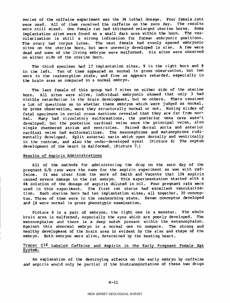
series of the caffeine experiment was the 3% lethal dosage. Four female rats
were used. All of them received the caffeine on the zero day. The results
were still mixed. One female rat had thickened enlarged uterine horns. Some
implantation sites were found as a small dark area within the horn. The vas-
cularization is still a strong indication for former embryonic positions.
The ovary had corpus lutea. The next female had evenly spaced embryonicsites on the uterine horn, but were unevenly developed in size. A few were
dead and some of the living embryos were malformed. Six sites were observed
on either side of the uterine horn.
The third specimen had 17 implantation sites, 9 in the right horn and 8
in the left. Ten of them appeared as normal in gross _bservation, but two
were in the reabsorption state, and five as appears retarded, especially in
the brain area as compared to a normal embryo.
The last female of this group had 7 sites on either side of the uterine
horn. All sites were alive, individual embryonic showed that only 3 had
visible retardation in the brain development, but no others. There remained
a lot of questions as to whether these embryos which were judged as normal,
by gross observation, were they structurally normal or not. Making slides of
fetal specimens in serial cross sections revealed that they are far from nor-
mal. Many had circulatory malformations, the posterior vena cava wasn't
developed, but the posterior cardinal veins were the principal veins, also
single chambered atrium end ventricles. Paired dorsal aorta and anterior
cardinal veins had malformalities. The mesonephrose and metanephrose rudi-
mentally developed. Split external naris which open dorsally and ventrically
in the rostrum, and also the under-developed eyes! (Picture 6) The septum
development of the heart is malformed. Picture 7.)
Results of Aspirin Administrations
All of the methods for administering the drug on the zero day of the
pregnant S/D rats were the same for the aspirin experiment as was with caf-
feine. It was clear from the work of Smith and Vacante that 12% aspirin
caused severe damage to the rat embryo. This experimentation started with a
6% solution of the dosage of aspirin diluted in oil. Four pregnant rats were
used in this experiment. The first rat uterus had excellent vasculariza-
tion. Each uterine horn had ten implantation sites, all together, 20 concep-
tus. Three of them were in the reabsorbing state. Seven conceptus developed
and i0 were normal in gross phenotypic examination.
Picture 8 is a pair of embryos, the right one is a monster. The whole
brain area is malformed, especially the eyes which are poorly developed. The
mesencephalon and there is a deep notch present within the metencephalon.
Against this abnormal embryo is a normal one to compare. The strong and
healthy development of the brain area is evident by the size and shape of the
embryo. Both embryos were alive, determined by the beating heart.
Tracer C14 Labeled Caffeine and Aspirin in the Earl[ Pregnant Female Rat
S[stem.
An explanation of the destroying effects on the early embryo by caffeine
and aspirin would only be partial if the biotransportation of these two drugs
H-II
NEW JERSEY GEOLOGICAL SURVEY

was not investigated. It was planned that radioactive labeled aspirin andcaffeine would be tested.
The drugs were administered by the gavage needle; four rats received caf-
feine, and four received aspirin. The rats were sacrificed 18, 24, and 48
hours after administering the labeled drug. The fourth rat was injected on
the eighth day of pregnancy and sacrificed 6 hours later. We used these
times since Smith and Vacante, 1976, used the 6, 12, and 24 hour timing; we
wanted to compare our results to make them conclusive, while also receiving
new pertinent information about the pathway of these two drugs.
From the sacrificed rats, six organs were remo-od and prepared for radio-
active readings. The brain was selected since both drugs affect the brain
which receives substantial vascularization. The second organ is the liver.
This organ was selected for the reason that any substance absorbed into the
blood stream must enter into the liver via the hepatic-portal system, also
the liver is the first and major filter of the body against all harmful drugs
and chemicals. The third choice was the kidney because the blood is filtered
there, where toxic wastes are removed and the kidney is of mesodermal ori-
gin. The remaining three organs are the ovaries, oviducts, and uterus. The
purpose was to see if the drugs were absorbed by these organs and to what
extent. All organs were prepared for the radioactive reading in the same
manner. For the labeled caffeine study, each rat received .04mg and .05mci
of radioactive drug; for the labeled aspirin study each received .04mg and
.05mci. The metabolic breakdown of aspirin or salicylic acid occurs in three
steps:
COOH
/OCOCH 3
i) salycilovic acid, 2) Ether or salycilate (Phinolic glucuramide) and
3) Ester of salycilate (Acylglucuramide). Part of the metabolic product is
oxidized to geutisic acid, the metabolites found in urine. Salicylates are
excreted by the kidney, and only a small portion leaves the body as a metabo-
lite, staying in the body for one or two days.
Caffeine is a methylated purine which has stimulating effect on the cen-
tral nervous system. Its structure is:
0 ICH3II N
N, .H
i N
CH3
The caffeine is also a weak stimuli for gastric secretions.
H-12
NEW JERSEY GEOLOGICAL SURVEY

At this time we were interested to know with the aspirin and caffeine,
when administered into the stomach and had gone through the metabolism, did
they reach the target organ? In what dosage? Also, what" concentration was
present after a specific time? The C14 labeled caffeine and aspirin werepurchased from New England Nuclear (NEN) .
In 1976, Szebenyi, Smith and Vacante used C14 labeled aspirin and caf-feine in the body, introducing the drug into the system and sacrificing 6,
12, and 24 hours later. They used the following list of tissues: brain,
liver, spleen, ovaries, oviducts, and uterus. According to their experiment
the highest reading for aspirin after 6 hours was in the ovaries at 148, ovi-
duct next at 92, uterus 38, spleen 16, liver 6, and brain 2. After 12 hours
the highest reading was in the uterus at 362, and after 24 hours the highest
reading was still in the uterus but in a lower concentration at 60.
The labeled caffeine after 6 hours was read and found to he the highest
in the oviduct at a reading of 198, next the ovaries at 168, uterus 66,
spleen 12, brain 10 and liver 7. At 12 hours after administration the ovi-
duct had a reading of 312, ovaries 202, uterus 90, spleen 14, brain 8, and
liver 2. Finally at 24 hours the ovaries again had the highest reading of
126, then the oviduct at 106, uterus 36, spleen and brain 4, and liver 2.
This data suggest that the highest concentration of the labeled drugs accu-mulated in the genital system.
Szebenyi, Smith and Vacante used only non-pregnant females in the radio-
tracing experiment. In this years' experiment, we decided to check the accu-
mulations of the two labeled drugs in fertilized females at 18 hours, 24
hours, 48 hours, and also a pregnant rat on the eighth day of pregnancy and
gavaged 6 hours before it was sacrificed as mentioned earlier.
In this year's research a different technique was used from the 1976
experiment for radioactive reading. After removing the organs we chose from
the pregnant rat, they were homogenized and mixed with .9% sodi_ chloride to
a fixed value. Tables III and IV. At St. Mary's Hospital, under the super-
vision of Dr. Hordynsky, the samples were centrifuged at 2200 rpm for ten
minutes. One millimeter of the supernatant was removed and then was mixed
with either 5 or i0 cm3 of a phosphorous cocktail solution. We read the
emission for one half a rain, in a machine designed to count C14 radiation
in solutions. This technique appeared more accurate than last year's ashing
technique because some of the C14 radiation could escape as a volatile
hydrocarbon, thus influencing the reading unless very strict procedures were
followed. After computing the readings to counts per minute per gram of the
tissue and percentage present in comparison to the oviduct, we got the fol-lowing results. In the labeled aspirin experiment, the 18 hr. rat had the
highest concentration in the oviduct at 600, next the uterus at 440, ovaries
400, kidney 156.5, brain 75, and the liver the lowest at 17.2. The 24 hr.
rat had the highest readings in the uterus at 1200, next the oviduct and the
ovary with 1000, the brain 153.8, kidney 75 and the liver with the lowest
reading at 21.6. The 48 hr. rat had the highest reading in the oviduct with
2000, ovaries 400, uterus 200, brain 81.1, liver 66.6 and kidney with 6.6.
The 8 day rat had its highest reading in the oviduct with 2800, uterus
1946.7, ovaries 1733, kidney 1109, brain 191, and liver 107. (See table Ill.)
H-13
NEW JERSEY GEOLOGICAL SURVEY

In the labeled caffeine experiment the following results were observed.
The 18 hour rat had the reading in the oviduct at 8000, ovaries 2400, uterus
1120, kidney 360, brain 185, and liver 158. The 24 hour rat we had to leave
out because we had a large % error and we felt that it made this data
invalid. Se Table I and II for absolute reading of labeled aspirin and caf-
feine experiments. The 48 hour rat again had the highest concentration in
the oviduct at 1400, ovaries 800, uterus 333, brain 188, liver 140, kidney
107. The 8 day pregnant rat, after administration of the labeled caffeine
was found to have the highest ooncentration in the brain at 2957, uterus
2733, ovaries 2300, oviduct 2000, kidney 463, and liver with 372. (See Table
IV). To summarize the results of the labeled caffeine and aspirin experi-
ment, the readings were calculated into a percentage where the oviduct read-
ing was equivalent with 100 percent. In the labeled caffeine experiment,
Table IV, it is clear that of the organs examined the oviduct, ovaries, and
uterus showed the highest readings among all the organs consistently. Spe-
cial attention can be given to the 8 day old pregnant which was at 38% of her
gestation time, more than 1/3, and here the uterus with the implanted embryo
had the highest reading with 2733 counts per gram. At this point mention
must be noted that it wasn't investigated which, the uterine wall, the pla-
centa, of the embryo of these absorbed the drug and it wasn't investigated if
these embryos are affected at this point of development if the drug is admin-
istered this late time of pregnancy.
In the labeled aspirin experiment, Table III, that out of the organs
examined the oviduct, ovaries and uterus again had the highest readings and
the oviduct was the highest except in the 24 hour reading where the uterus
was found with a reading 20% in excess of the oviduct.
The dosages of 6% and 3% were used in this experiment. These were calcu-
lated from the lethal dosage and at this amount it is considered low. Fur-
ther experimentation with labeled drugs can also give light whether the
males' genital organs collect higher concentrations of salicilates and caf-
feine. If it does, maybe the pathways and reasons for high concentration in
these organs can be seen more clearly.
"Earth engendered the members most grotesque;
Monsters, half-man-half-woman, footless and
handless, void of mouth or eye ....
Nature checked their vile growths ....
Hence, doubtless, many a tribe has
sunk suppressed, powerless its kind to breed.--
Einpedocles 495-435 B.C.
DISCUSSION
In the issue of Science November 26, 1976, was an editorial "Irrational
Drug Prescribing and Birth Defect." The article is an important one and itstates:
H-14
NEW JERSEY GEOLOGICAL SURVEY

"Few physicians receive formal training in the correct use of drugs,
but the average practitioner writes 7,934 prescriptions each year.
Many of these prescriptions are irrational in the sense that the drug
has not been shown to be effective for the purpose for which it has
been prescribed, many are completely inappropriate because they rep-
resent a substantial hazard to the patient without any compensatingbenefits."
This article is an argument against the unnecessary drug uses by the physi-
cians. The drugs are used frequently and some times with no experimentation
against side effects. Therefore this makes more important, the animal exper-
imentations which were introduced by Hale and then in larger scale by
Warkany. By 1961 it was known to the teratologist that many drugs, including
salicylates are teratogens when given at the right time, in the right dose to
the right animals. In recent times caffeine came into the focus of the tera-
togenic research, which now strangely suspects that the caffeine had terato-
genic effects in the human. This experimentation deals with the two most
commonly used human drugs, caffeine and aspirin, to prove they have terato-
genic effects on animal models. In 1970 Bartholomew reported that the caf-
feine has positive mutagenic effects. The most dangerous among the many
mutagenic drugs are these which can cross the placenta as free drugs. Among
those are the salicylates and the caffeine. Evans states that (1975) -
Probably the most critical factor involved in drug-induced teratogenesis is
in the utero age of the developing fetus. In a figure they show the adult
female to have teratogenic susceptibility. In this chart they believe that
the first 20 days of human development, the so-called "pre-differentiation"
period is usually not susceptible to teratogenesis. They also stated, Organ-
ogenesis in humans begin about the twentieth day of gestation (the first
somite stage) and continues for the most part through the third month. The
risk of morphologic analysis is therefore greater during the first trimester
(day 20-day 90) cie. during the period of the greatest organ development.
Harbijou and Becker 1972 used DPH in the rat. If the drugs were administered
during early gestation (day 7-10), hydronephrosis was the prominent morpho-
logical observation. However, administration on days 10 through 14 resulted
in cleft palate formation. This categorical determination that the early
embryonic life, (before the first somite) is not sensitive for the terato-
genic effect of a drug is not an overall truth. It can be certainly true for
the drug DPH, but not so for other drugs. It must be recalled the experiment
with the rats, when the drug was administered on the zero day of pregnancy,
its effects were more damaging when the drugs were administered through the
half time of the pregnancy.
In this paper the embryos were in the earliest stage possible, there was
no connection at this time with the maternal blood supply, it was possible to
be able to enter in the upper third of the oviduct of the mother. Then an
important question arises, how can the administered drug influence the early
one cell stage preimplantation embryo? The possible answer may be from the
results obtained by the radioactive labeled drugs. Why were both the caf-
feine and aspirin accumulating around the ovary, oviduct, and the uterus in
the highest level; why are they not neutralized by the liver for excretion?
When the drug administration occurred, the zygote still was covered with the
corona radiata, and the follicular cells. It is possible that the follicular
cells transported the chemical into the zygote? Certainly not is the
answer: the follicular cells are separated from the maternal organism just
H-15
NEW JERSEY GEOLOGICAL SURVEY
like the zygote itself. But the tubat fluid is labeled the zygote with the
surrounding corona radiata and this way maybe the follicular cells can pick
up some of the part of the drugs. It is not proven yet but this can be the
project to the next experiment to establish the route of the drug to the pre-
implantation embryo.
This experiment has the conclusions only for the Rattus norvegicus albi-
cans and not in any way to apply for the human population. Many reasons canbe listed which make the animal results not suitable for human condition.
First the greater degree of inbreeding in any strains of laboratory animals
than in the man, for example, the different metabolism of drugs in man com-
pared to other mammals. The possible protective effect of the larger size
and larger gestational period of the human fetus.
A one-day exposure to a drug, for instance, affects about 1/21st of the
embryonic period of a mouse but only about 1/26th of the comparable period in
the human. On the other hand, malformations of the human fetus might pos-
sibly result from massive doses of certain drugs given during a major part of
the embryonic period, which fortunately are rarely administered to pregnant
women in that fashion. If the reader agrees with Irvin Emanuel (1976) then a
question arises in this experiment.
The preimplantation periods are similar in the mouse, rat, rabbit, in man
and many other mammals. These 5 days of development are the same, and five
days in some animals as development are concerned with be equivalent with 5
days in the other animals. During this time there is no organ differentia-
tions, the five day term and in all of the cases with the development of the
blastocyst stage. (Picture 9). this shows the four day old preimplantation
embryo in the rats. This picture was taken in this laboratory, can be com-
pared with any human embryology book development stage the hour day old human
blastocyst stage confusingly similar. This also means that during this four
day journey before the implantation is true in all mammals and can he com-
pared on a day to day basis.
But to compare the drug effect is certainly not in the scope of this
paper.
AC_O_EOGEMENT
My thankful appreciation to my many students who helped to carry out this
chain of experiments since 1971. Without their enthusiastic and responsible
work, the results could not be reached.
BIBLIOGRAPHY
Carr, D.H. Chromosomal Anamolies as a Cause of Spontaneous Abortion Am.J.
Obstet. Gyn. 97:676-682. 1962.
Daniel, J.C. ed. Methods in Mammalian Embryolo@y (San Francisco: W.H.
Freeman and Company) 1971.
H-16
NEW JERSEY GEOLOGICAL SURVEY

Fraser. Experimental Teratogenesis in Relation to Congenital Malformation in
Man. In Second International Conference of Con@enital Malformations. M.
Fischbein, ed. (New York: The International Medical Congress Ltd.)1964.
Goodman and Gilman. Pharmacological Basis of Therapeutics. (New York: TheMacmillan Co.) 1975.
Hamburger, V. A Manual of Experimental Embryology. (Chicago: TheUniversity of Chigago Press) 1962.
Inborn, S.L. Chromosomal Studies of Spontaneous H_an Abortions. Advanced
Teratology. D.H.M. Woollam, ed. (New York: Academic Press) 2: 37-39.1967.
Kallen, B. Early Morphogenesis and Pattern Formation in the Central Nervous
System. Organogenesis. R.L. Dehaan and H. Ursprung, eds. (New York: Holt,
Rinehart and Winston) 1965.
Kappas, A. and A.P. Alvares, How the Liver Metabolizes Foreign Substance
Scientific American. 232:22-31. June, 1975.
Mann, L. et al. Thalidomide in Rabbit Semen. Nature 214:1018-1020. 1967.
Moore, L.E. The Developing Human (Philadelphia: W.B. Saunders Co.) 1973.
Saxen, L. and J. Rapola. Con@enital Defects. (New York: Holt, Rinehart andWinston Inc.) 1969.
Thompson, J. and M. Thompson. Genetics in Medicine. (Philadelphia: W.B.
Saunders Co.) p. 249-250. 1973.
Warkany, J. Congenital Malformations. (Chicago: Year Book Medical Publisher)1971.
H-17
NEW JERSEY GEOLOGICAL SURVEY

coIf_ kD D-
O ° O _S O• 04 04 ,-t •
+_ ," OO _ OoD O • O.i-
IEI.,-I
_ O f'_ PJ r--I O
•. oo - o. - o . ooID H r-_ CO O Oh ,-_ '.D O _:# (klO _ rHOJ
U
6,, ° ,_ o O.--_ ,, ORO O ,' Ot, D
0 iN)
-,_ _ ',D OJ O,_ t_ O ,-I O ¢,n
I1; _' O'_D " O00 ,' O _ OkO_i CO r-I Lr_ O CO ,-'t 0,10 _ _-IO Lr_ OJr-I
4J
0 i _ o o
m _-I 0 • 0 co,_ ',D • .-4 _•_ OkO ,--I O O O O.I O _" O Oq
Lr_ f,_ O ,-I I.rx OJ C_ ,--I Lr_o ,--t Lr_ _--I
4_
O _ '..O -_ O
•1:_ ,--I 0 ,-I O
_ ,--I r--t CO-P OJ 0-_ 0 Lr_Ro 0 ,' 0 0'_
I O o•el .rt
H _ +_
F_ m t_ _ m m_ _ m m 0 m m 0
a_
H-18
NEW JERSEY GEOLOGICAL SURVEY

• ° o43 0J O OJ OJ
0¢J O_ OOJ _ 0 • 0 0 kD 0I_ r'-I O_r-I OJ Oq_O Oq Cq Oq eq
'H
¢;
X
% 0
p_ GO O • Oq O O Ox O Lr', O,--t ,--IMD O3 r-'! OJ OJ r--I Oq r-t
'<
O,-4
o _; o g 20 • _,_ 0 0 00 ,--I r-I .._ O.I HCO (M ,--I Oq ,--I
,H
I_ 0 0
• ,-4 OOJ OO b-- O O+_ _-I r-{CM C_I r-I r-I OJ _-I I ('I r-I I
O
,-'I e-t 0 r-I H0 O "
•._ _ O O O.::t _5) O 04 OE-_ ,-I Lt'_.-_r OJ Lrx,-I OJ Lrx I eq LP_ I
0
i "_:) O0J O_ L_O3 Lrx O ,-q OI H rl _-I _-_ _-I r-I .I OJ _1 I _ r-I I
H O 0 0 0
_ ,_o _,_o _ _o _ ,_o
-,-I.H _ , .Pl .H O] , ._I-H * .,-I._
_ "_ _.._=_ _ "_ _ "_"_• o ._ o o O.H o o 0 .H • 0-_
H-19
NEW JERSEY GEOLOGICAL SURVEY

,H
_ O_ kidkO b'_ _D 0
kid _ o_ ,--4 O_(M I_- _-- _D _ O_
_ 0 0 0
_ 0 0 0
O_
_ -_ 0 0 0 0
°° i•_ 0 0 0 0
i0 _ _ _ _
m_°_
O0 "_ _ " _ _ °
_ •
_ o _ o _ o _ o
_._ _._ _._ _-_
_00 _ _00 _ _00 _ _00
H-20
NEW JERSEY GEOLOGICAL SURVEY

_N
_ 0 0 0%_ 0 0 0O_ 0 _ 0
o _ I I M I _ I
O_
_ 0 0 0 _O_ _ 0 0 _ _
0
°_
_°H 0 _
0
_0 _ _ 0 _0 _ _ _ _
_0
O0 _ ° _ _ _ _
_ •
_ 0 _ _I 0 _ 0
_ 0 _ _1 _ 0 _ _ 0
H-21
NEW JERSEY GEOLOGICAL SURVEY

NEW JERSEY GEOLOGICAL SURVEY

NEW JERSEY GEOLOGICAL SURVEY

NEW JERSEY GEOLOGICAL SURVEY

NEW JERSEY GEOLOGICAL SURVEY

NEW JERSEY GEOLOGICAL SURVEY
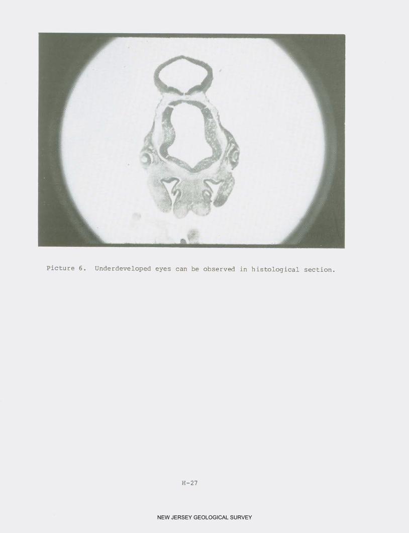
NEW JERSEY GEOLOGICAL SURVEY

NEW JERSEY GEOLOGICAL SURVEY

NEW JERSEY GEOLOGICAL SURVEY

NEW JERSEY GEOLOGICAL SURVEY

EXTREME RUNOFFS IN REGIONS OF VOLCANIC ROCKS IN CENTRAL EUROPE
AND IN NORTHEASTE_ U.S.A.*
by
Dr. GEORGE J. HALASI-KUN
Chairman, Columbia University Seminar on Pollution and Water Resources
*Presented in the International Symposium on Hydrology of Volcanic Rocks,Lanzarote, Canary Islands, Spain, March 1974 as a contribution of Columbia
University Seminar on Pollution and Water Resources, New York City.
I-i
NEW JERSEY GEOLOGICAL SURVEY

(i) INTRODUCTION
Generally, it is accepted that--especially in smaller watersheds (up to
350 km2) and at similar climatic conditions--the extreme surface flows
(100-year maxima and minima) are depending mainly on the permeability of the
soil and the geologic subsurface including their saturation, the topographic
conditions (slopes) and the size of the watershed. As secondary factors for
peak runoffs are the yearly rainfall with its distribution, the point rain-
fall intensity, the storm characteristics, the retardation effect of the veg-
etative oover, the lake and swamp area and finally the roughness of the
surface.
The above factors are the most important elements governing the peak
flows. The coefficients of the lowest flows are slightly different. They
are depending also on permeability of the geologic subsurface and the size of
the watershed, but to a greater extent on the evapotranspiration than on the
slope characteristics (topographic conditions). The length of the drought,
the frequency and the amount of rain, the retardative effect of forest and
lake and finally the relative elevation of the watershed to the adjacent
region are the additional factors modifying the minimum flows.
Based on these principles, they were two areas investigated in the 1960's
and 1970's: East-Czechoslovakia in Central Europe and New Jersey in North-
eastern U.S.A. (i) and (2). In both cases, the above listed principles were
confirmed and extreme flow equations were established in accordance with the
various geologic formations. Since in both areas are geologic formations of
volcanic or plutonic origin, it has merit to describe the findings.
(2) HYDROGEOLOGIC DESCRIPTION OF THE VOLCANIC ROCKS IN THE CARPATHIAN BASIN
(EAST-CZECHOSLOVAKIA) AND IN NEW JERSEY, U.S.A.
In East-Czechoslovakia, the Central Slovak Carpathians mostly Paleozoic
Crystalline formations, Granite, Gabbro, Sandstones in the North and Mesozoic
Basalt, Andesite and Tuff in the South interwoven and surrounded mainly in an
arc form from West to East can be found. The general layout of volcanic
rocks of the area together with the geologic pattern of the adjacent region
is given in Fig. i. The yearly average rainfall varies from 750 mm in theSouth to 2100 mm in the North. The peak floods are caused either by trans-
continental cyclones or by local torrential rains. The point rainfall inten-
sity reaches 125 mm per day value. The recorded storm pattern is an
ellypsoid 15 km by 50 km, with the highest intensity in its focus (3). The
valleys' elevation is 400-700 m and the peaks of the mountains reach in theNorth 2600 m and in the South 1300 m elevation. Vegetative cover (forest) is
40%, the lake and swamp area is insignificant. Evapotranspiration amounts to
40% in the South and to 35% in the North of the yearly rainfall values.
The area can be divided into three hydrogeologic regions (4). The coarse
grained Granite and Gneiss, some times with Porphyry, Diabase and Trachytehave few local springs with a limited capacity up to 1 i/sec. On the other
hand, the Porphyritic Basalt and Andesite region is characterized by numerous
springs of little capacity up to 2 i/sec. The increased voids in this region
are only near to the surface, therefore, these springs of low yield can befound on various elevation and their location is quite scattered which makes
any substantial concentration of water supply extremely difficult. Water can
I-2
NEW JERSEY GEOLOGICAL SURVEY

be found mainly along contact lines of the various formations. Geologically
in some areas the Basalt and Andesite are mixed with Trachyte. The third
hydrogeologic region can be called the fine grained Andesite interwoven with
Tuff including some agglomerates etc. (Ryholite, Trachyte, Dacite etc.) and
Tuffite. The weather-beaten Granite and Gneiss areas chiefly on the southern
more fractured slopes and more exposed side of the formations and in areas of
accumulated piles of debris caused by weathering and erosion belong also to
this hydrogeologic region where the springs are generally in the lower part
of the depressions similar to the previous region: along contact lines of
the formations with a capacity up to 4 i/sec.
In New Jersey, U.S.A., there are two areas where rocks of volcanic or
plutonic origin can be detected (5). The bulk of the Appalachian Highland
Province in the North is formed by Precambrian Gneiss, Granite and Gabbro.
The Highlands are characterized by the flat-topped ridges which have an aver-
age elevation of 300 m above sea level. These are cut by narrow, steep-sided
valleys 60 to 240 m below the summit level. Between the Highlands and the
Coastal Plains, the Piedmont Province is comprising the central part of the
State and has in Northwestern part extrusive Triassic Basalt (Watchung Basalt
lava flows at some points accumulated to a total thickness of 240 m). Along
the Hudson River intrusive Triassic Diabase sill (300 m thick) is dominant
which reappears in the Southwestern part of the Piedmont. The ridges have a
200 m elevation and the valleys are at 50 m above sea level. Fig. 2 gives
information about the igneous rocks and other geologic formations of New
Jersey. The yearly average rainfall is 1125 mm. The peak runoffs are caused
by local thunderstorms, cyclonic continental storms or extratropical storms
(hurricanes). The point rainfall intensity reaches 250 ram/day value. The
recorded storm pattern area is 30 km by 105 km. The vegetative cover (for-
est) is 47%; the lake and swamp area is in general 2% and reaches up to 17%
in some areas. Evapotranspiration amounts to 45% of the yearly rainfall (500
ram) (6).
The volcanic formations in New Jersey have also three hydrogeologic
regions but less differentiable than those in East-Czechoslovakia. The
groundwater is available only to a depth of 180 m below the surface. Boring
tests proved that below that level there is a very marked decrease in frac-tures and fissures from which water can be obtained. There is also evidence,
of course, that certain fracture zones may give abundant water at great
depth, but these fractures are those such as the Precambrian-Triassic border
fault or others that have been mapped for years. The coarse grained Granite,
Gneiss and Gabbro area can be divided into two hydrogeologic regions. The
whole area is distinguished by rugged topography with numerous springs and
shallow wells of various capacity from less then 1 i/sec up to 4 i/sec which
can be even increased by widespread stratified deposits of glacial origin.
It must be pointed out that the uneven surface weathering divides this geo-
logic province into two hydrologic regions in the area of the Precambrian
formations: one with very limited amount of voids where springs and wells
have a capacity only less than 1 i/sec; the other one with substantially more
interstices and fractures where springs and wells reach the capacity up to 4
i/sec. The first region, therefore, can be described as poor in voids and
fractures, consequently poor in water. The Biotite Gneiss, Amphibolite,
Pyroxene Granite and Skarn are the most distinctive formations. The other
region is the area of the weathered igneous rocks of the same formations and
I-3
NEW JERSEY GEOLOGICAL SURVEY
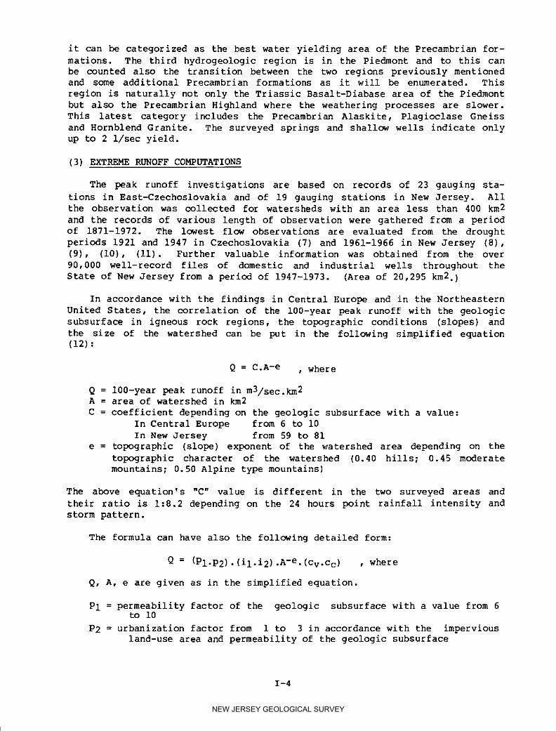
it can be categorized as the best water yielding area of the Precambrian for-
mations. The third hydrogeologic region is in the Piedmont and to this can
be counted also the transition between the two regions previously mentionedand some additional Precambrian formations as it will be enumerated. This
region is naturally not only the Triassic Basalt-Diabase area of the Piedmont
but also the Precambrian Highland where the weathering processes are slower.
This latest category includes the Precambrian Alaskite, Plagioclase Gneiss
and Hornblend Granite. The surveyed springs and shallow wells indicate only
up to 2 i/sec yield.
(3) EXTREME RUNOFF COMPUTATIONS
The peak runoff investigations are based on records of 23 gauging sta-
tions in East-Czechoslovakia and of 19 gauging stations in New Jersey. All
the observation was collected for watersheds with an area less than 400 kin2
and the records of various length of observation were gathered from a period
of 1871-1972. The lowest flow observations are evaluated from the drought
periods 1921 and 1947 in Czechoslovakia (7) and 1961-1966 in New Jersey (8),
(9), (i0), (ii). Further valuable information was obtained from the over
90,000 well-record files of domestic and industrial wells throughout the
State of New Jersey from a period of 1947-1973. (Area of 20,295 km2.)
In accordance with the findings in Central Europe and in the Northeastern
United States, the correlation of the 100-year peak runoff with the geologic
subsurface in igneous rock regions, the topographic conditions (slopes) and
the size of the watershed can be put in the following simplified equation(12) :
Q = C.A-e , where
Q = 100-year peak runoff in m3/sec.km2A = area of watershed in km2
C = coefficient depending on the geologic subsurface with a value:
In Central Europe from 6 to 10
In New Jersey from 59 to 81
e = topographic (slope) exponent of the watershed area depending on the
topographic character of the watershed (0.40 hills; 0.45 moderate
mountains; 0.50 Alpine type mountains)
The above equation's "C" value is different in the two surveyed areas and
their ratio is 1:8.2 depending on the 24 hours point rainfall intensity and
storm pattern.
The formula can have also the following detailed form:
Q = (Pl.P2).(il.i2).A-e.(cv.Cc;) , where
Q, A, e are given as in the simplified equation.
Pl = permeability factor of the geologic subsurface with a value from 6to 10
P2 = urbanization factor from 1 to 3 in accordance with the impervious
land-use area and permeability of the geologic subsurface
I-4
NEW JERSEY GEOLOGICAL SURVEY

iI = twenty-four hours point rainfall intensity coefficient from 0.5 to
2.0 (0.5 for 35 mm/day; 1.0 for 125 mm/day; 2.0 for 250 mm/day)
i2 = storm characteristic with a value from 1 to 4.1 depending on the
size and pattern of the extreme storms and on the wind velocity
cv = coefficient of the vegetative cover from 0.95 to 1.05 (from 40% to70% forested of the watershed)
ce = concentration coefficient from 0.90 to 1.05 (0.90 for elongatedshape or at least 1:5; 0.95 for horseshoe shape and 1.05 for
fan-shaped watersheds)
The roughness of the surface and its retardation effect-on the flow is not
treated separately because this phenomenon is bound on the geological forma-
tion. Therefore, this effect is part of the geological runoff coefficient
"C" in the simplified equation and of permeability factor "PI" in the
detailed formula. Both basic equations are developed for Central Europe when
the parameters have a unit value (i.0) except coefficient "C" and exponent
"e". The values of coefficient "C" in volcanic formations of the both areas
are given in Fig. 3.
The lowest runoff formula has a similar form
Q = C.A-e , where
Q = lowest runoff (50-year runoff ?) value in i/sec.km2A = area of watershed in km2
C = coefficient depending on the geological subsurface with a value from
0 to 2 (Fig. 4):
In Central Europe from 0-i.i to 2
In New Jersey from 0-1.7 to 0.9
e = 0.065--the exponent indicates an almost even distribution of the low-
est runoff regardless of the size of watershed and the available data
and values were not sufficient evidence to evaluate the influence of
slopes and topographic configuration of the drainage basins in fur-ther details.
On the other hand, the constant value of the exponent "e" and the different
values of the coefficient "C" in the two surveyed areas indicate that the
lowest runoff is more depending on the e_apotranspiration effect (% of yearly
rainfall) than on the slope characteristics since the minima occur at the end
of the drought period when the stored groundwater is less bound on the topo-
graphic characteristics of the watershed than on the evapotranspirationeffect.
(4) CONCLUSION
The developed equation for peak runoff in smaller watershed with an area
less than 300 km2 can be considered for computations of 100-year peak run-offs. The formula of lowest runoff can be used for areas less than 50-100
km2 and only for a 50-year lowest flow value because of insufficient lengthof observation further details and refinements of the formula could not be
achieved.
I-5
NEW JERSEY GEOLOGICAL SURVEY
BIBLIOGRAPHY
i. Balasi-Kun, G. J. (1968) . Die Ermittlung yon H6chstabfldssen fur
Einzugsgebiete kleiner als 300 kin2 in Bereich der Slcwakei--Methoden
und Verfahren, Braunschweig, Technische Univer sitat--Leichtweiss-Institut.
2. Halasi-Kun, G. J. (1972). "Data Collecting on Water Resources and Com-
putations of Maximum Flood for Smaller Watersheds," Simposio Inter-nacional Sobre la Planificaci6n de Recursos Hidraulicos--Ponencias,
Volume I, Mexico, Secretaria de Recursos Hidraulicos.
3. Halasi-Kun, G. J. (1949). Hydrologia, [(o_ice.
%, V
4. Hynie, O. (1961). Hydrogeologie CSSR, Prague, Nakladatelstvi Cs.Akademie Ved.
5. Widmer, K. (1964). The Geology and Geography of New Jersey, Princeton,D. Van Nostrand.
6. Climatological Data of New Jersey (1971) . Washington, D.C., U.S.
Department of Commerce, National Oceanic and Atmospheric Administration,Environmental Data Service.
7. Dub, O. (1957) . Bydr ologia, hydrografia, hydrometr ia, Prague-Br atislava, SVTL.
8. Kasabach, H. F. (1966). Geology and Ground Water Resources of Hunterdon
County, Special Report 24, Trenton, State of New Jersey.
9. Miller, J. (1973). Geology and Ground Water Resources of Sussex
County .... , Geol. Bulletin 73, Trenton, State of New Jersey.
10. Widmer, K. (1965). Geology of the Ground Water Resources of Mercer
County, Geol. Report 7, Trenton, State of New Jersey.
ii. Water Resources Data for New Jersey" 1961-1973, Part i: Surface Water
Records (1962-1974). Trenton, U.S.G.S.
12. Halasi-Kun, G. J. (1974). "Computation of Extreme Flow and Ground Water
Capacity with Inadequate Hydrologic Data in New Jersey," Proceedings of
University Seminar on Pollution and Water Resources, Volume V, 1971-1972, New York--Trenton, Columbia University.
I-6
NEW JERSEY GEOLOGICAL SURVEY

I-7
NEW JERSEY GEOLOGICAL SURVEY

I ,J _ GEOLOGIC MAP
• ' _r OFNEW JERSEY
DE LAWARE 1959BAY
Figure 2. Igneous Rocks of New Jersey (1959)
I-8
NEW JERSEY GEOLOGICAL SURVEY

Hydrologic Regions: Peak Runoff Coefficient in m3/sec.km2(formations) in Central Europe: in Northeastern U.S.:
(i) Granite, Gneiss 10 81
(2) Basalt-Andesite
(Central Europe) 8Basalt-Diabase
(Northeastern U.S.) 70
(3) Weathered Igneous Rock
(Tuff with agglomerates) 6 59
Figure 3. Peak Runoff Coefficient in Volcanic Rocks
Hydrogeologic Regions: Lowest Runoff Coefficient in i/sec.km2
(formations) in Central Europe: in Northeastern U.S.
(I) Granite, Gneiss less than 0.7* less than 0.4
(0 to i.i_ (0 to 1.7)
(2) Basal t-Andesite 1
(Central Europe) (0.5 to 1.5)
Basalt-Diabase) 0.6
(Northeastern U.S.) (0.17 to 0.0)
(3) Weathered IgneousRock (Tuff with
agglomerates) 2 0.9
*Alpine type areas (frozen most of the year) are excluded.
Figure 4. Lowest Runoff Coefficient in Volcanic Rocks
I-9
NEW JERSEY GEOLOGICAL SURVEY

HACKENSACK RIVER
DETERMINATION OF TERTIARY SE_%GE TREATMENT
REQUIREMENTS FOR _STE _TER DISCHARGE
by
Dr. RICHARD W. LO PINTO,* CHESTER P. MATrSON,** and JOANNE D. LO PINTO ***
*Dept. of Biology, Fairleigh Dickinson University, Rutherford, New Jersey07070.
**Hackensack Meadowlands Development Commission, 1099 Wall St. West,
Lyndhurst, New Jersey 07071.***Lo Pinto AssOciates, Inc., 88 Willow Avenue, Hackensack, New Jersey
07601.
J-i
NEW JERSEY GEOLOGICAL SURVEY

INTRODUCTION
The addition of phytoplankton stimulating nutrients into any body ofwater, via domestic waste water effluents, has the potential of significantly
reducing dissolved oxygen levels in the water. This, in turn, brings about a
reduction in the number and diversity of desirable life forms and creates an
environment which favors the proliferation of biological and chemicalpathogens.
The value of removing specific algae promoting nutrients from sewage has
increasingly become recognized, especially as we experience an increased vol-ume of waste water flow into rivers, lakes and estuaries, and as a favorable
ecological balance in these areas declines. However, enthusiasm for achiev-
ing "total effluent purity" must be tempered by an understanding of which
nutrients and other effluent components in fact damage the environment and to
what degree natural and economic resources are affected. This is implied in
the Federal Water Pollution Control Act of 1972 which admonishes that any
proposed method of sewage treatment be environmentally sound and cost effec-
tive. Direct and indirect costs are a major consideration because the con-
struction and operation of a waste treatment facility may result in changes
in air quality, land use planning and energy utilization.
This report deals with the necessity for constructing a tertiary sewage
treatment plant on an area of the Hackensack River near Secaucus, New Jersey,
by analyzing the effect of two chemical nutrients, nitrogen and phosphorous,
which have been shown in other bodies of water to be responsible for eutrO-
phication and which can be removed from domestic waste water by tertiary
treatment. It is important to note that individual eco-systems respond in
different ways to these elements. For example, a nutrient such as phospho-
rous which causes excess algal growth in one of the Great Lakes has littleeffect in areas of Long Island Sound, where it is nitrogen that is responsi-
ble for eutrophication.
It is evident then that chemicals that are potentially stimulatory to
algal growth must be investigated on an area basis. Differences in response
of each area to specific chemical agents can he attributed to environmental
modification by industrial waste, landfills, sewage outfalls, microbial popu-
lations and the fauna and vegetation of adjacent terrestrial, marsh and
aquatic areas.
The economic benefits of determining and removing eutrophicating agents
from sewage treatment effluent are evident. Recreational utilization of
receiving waters are safeguarded, and adequate water quality is maintained to
accomodate commercially valuable marine fish that utilize marshes as nursery
grounds.
The economic advantage associated with determining that tertiary treat-
ment is not necessary is more directly apparent. The millions of construc-tion and maintenance dollars necessary to support such a facility can be
saved while at the same time retaining recreational and asthetic benefits.
J-2
NEW JERSEY GEOLOGICAL SURVEY

MATERIALS, METHODS & DISCUSSION
Water samples used in the eutrophication analysis were collected in chem-
ically clean containers and refrigerated prior to being processed. All sam-ples were collected from the Hackensack River in Northern New Jersey near the
base of the Erie Lackawanna Railroad Bridge and this study and its evaluationis indicative of conditions in this limited area.
A portion of the water sample was filtered thru a 0.45 micron milliporefilter. To this were added the chemicals, individually or in combination,
that were under investigation as potential limiting factors. The enriched
and unenriched water samples were then inoculated with phytoplankton indige-nous to the area from which the sample water was obtained.
Experimental and control cultures was then incubated until phytoplankton
growth levels were sufficient to permit a meaningful evaluation of the
results. A significant stimulation of phytoplankton growth above control
levels caused by chemical enrichment of the water indicates that the chemical
used is a limiting factor. A failure to stimulate growth significantly
beyond the level of the control indicates that the chemical being tested is
not limiting and therefore, that its addition to the river water, as a compo-
nent of a sewage treatment discharge, will not stimulate excessive phyto-
plankton reproduction.
Tests for limiting factors were conducted throughout the year, rather
then just in the warmer months, because in shallow waters growth may never be
seriously limited by reduced solar radiation (Riley, 1969).
Ammonium, nitrate and phosphate were analyzed as suppliers of nitrogen
and phosphorous because they have been identified as being responsible foreutrophication in other bodies of water (Ryther & Dunstan, 1971) and because
of their known significance in estuarine algal physiology (Lo Pinto, 1972).
A broad spectrum of meadowlands phytoplenkton was utilized in each anal-
ysis. In this way, the interrelationships among the diverse populations are
not artificially eliminated. Provasoli (1963) has demonstrated that many
algae produce antibiotic substances which are capable of inhibiting the
reproduction of other algal species. An experimental system designed to
determine the presence of a limiting factor that selects against these inter-
actions by utilizing uni algal cultures may not accurately reflect environ-
mental conditions. Because interactions do occur in natural ecosystems, asystem of analysis for limiting factors in which phytoplankton populationsare tested in mixed culture insures a more accurate reflection of in situbiological responses.
Another refinement of our analysis is designed to avoid possible mis-
interpretation of nitrogen data. Ammonim, nitrogen has been shown to be toxic
to some phytoplankton even at very low levels but stimulatory to otherspecies at very high concentrations (McLaughlin, 1957) . Lo Pinto and
McLaughlin (1974) have shown that high concentrations stimulate the veryabundant estuarine chrysomonad, Micromonas.
In order to assure a correct interpretation of our nitrogen analysis,
ammonimn nitrogen was added in a broad range of concentrations so that any
J-3
NEW JERSEY GEOLOGICAL SURVEY

ammonium toxicity would be apparent. As an additional safeguard, nitrogen
was supplied as nitrate. Thus any significant stimulation of primary produc-
tivity by nitrogen would be readily recognized.
RESULTS AND DISCUSSION
The water quality analysis oonducted from March thru December 1976 in thearea of the Hackensack River previously mentioned, is presented in the
enclosed tables and figures.
Table I presents the effect on primary production of several concentra-
tions of phosphate and nitrogen compounds. The figures_reflect the potential
of these compounds to stimulate algal growth throughout most of the year.
The effect on primary production is recorded as a percentage of production in
the control, i.e. unenriched waters (primary production equivalent to that inthe control is indicated as 100% of the control).
Figure I and table I show that throughout most of the year exogenously
supplied phosphate concentrations of 0.1, 0.5 and 1.0 rag% do not stimulate
phytoplankton growth beyond that shown in the control. Samples collected in
late June, early July and August do show an increasing stimulation of phyto-
plankton growth in response to the lower levels of phosphate supplied (fig. 2- 4).
Figure 5 and table I reveal a relatively uniform response throughout the
sampling period to nitrate as a nitrogen source. No significant stimulation
or inhibition was apparent.
A review of figure 6 and table I reveals that low levels of ammonium show
a mild stimulatory trend in samples V, VI, and VII (see figs. 2 - 4).
Figure 7 and Table II, which consolidate the data on seasonal trends of
stimulation by phosphorous and nitrogen sources illustrate more clearly thetrend towards increased productivity between June, July and August in phos-
phate and ammonium enriched cultures.
It should be emphasized, however, that neither the nitrogen or phosphate
sources supplied individually to the organisms in the water samples analyzed
during the simmer months when water temperatures are relatively high (table
III) or at any time throughout the sampling period causes an excessive
increase in primary production. In all cases, production in nutrient
enriched samples remains well below a two fold (200%) increase over the con-trol. This represents but a fraction of the 1100 to 3600% stimulation that
has been reported in other areas. In addition, it is important to note that
no synergistic stimulation results from combining ammonium and phosphate(table I) at any time of the year.
The minor trend toward increased primary production that is seen in sum-
mer samples when araaonium and phosphate are supplied in vitro (fig. i), prob-
ably reflects an increased depletion of these nutrients in the HackensackRiver at the site studied, by phytoplankton and adjacent marsh vegetation.
It may also indicate reduced inorganic regeneration rates, or both these fac-
J-4
NEW JERSEY GEOLOGICAL SURVEY

tors may be contributory. During the remainder of the sampling period physi-
ologically available phosphorous and nitrogen are apparently received by or
regenerated in the river at a rate which exceeds demand by autotrophs.
It is evident from our analysis that the decrease in eutrophication
potential that would be achieved by even total nitrogen and phosphorous
removal from any industrial or municipal waste water trea_ent facility,
intended to discharge in the Hackensack River in the area studied would pro-
vide no ecological advantage.
Indeed, the economic, energy and natural resource expenditures that would
be required to construct and maintain such a plant would represent a disCservice to the Hackensack River estuary.
In view of the results and conclusions expressed herein, it is evident
that the 1984 EPA goal of "zero pollutant discharge" may well be worthy of
reconsideration, at least for parts of the Hackensack River estuary. Fur-
thermore, it is also important to mention, in view of the increasingly popu-
lar utilization of mathematical models to predict the effects of pollutants,
that data of the type generated for this report need be included in the cal-culations that balance the benefits and risks of constructing waste watertreatment facilities. If this is not done it is conceivable that in some
circumstances natural and economic resources could unjustifiably be expended
in order to gain environmental goals which do not reflect the needs of the
particular ecosystem being considered.
BIBLIOGRAPHY
Lo Pinto, R.W. (1972) Physiological studies of axenic algal populations
isolated from a eutrophic biotope. Ph.D. Dissertation, Fordham Univer-sity, Bronx, New York
Lo Pinto, R. W. and J.J.A. McLaughlin (1974) Nutrition and physiology of a
gall marine Chrysomonad. J. Protozcology, 21, (3) 419.
Mattson, C., R. Trattner, J. Teal and I. Valiela (1975) Nitrogen import and
uptake measured on marshes of the Hackensack River in New Jersey. Paper
presented at the 38th Ann. Meet. Amer. Soc. Limnol. Oceanogr., Halifax,Nova Scotia.
McLaughlin, J.J.A. (1958) Euryhaline Chrysomonads: Nutrition and Toxigene-
sis in Prymnesiam parvam with notes on Isochr_sis @albana and Monochrllsislutheri. J. Protozcology, 5: 75-81.
Provasoli, L. (1963) Organic regulation of phytoplankton fertility. In M.
N. Hill (ed.) The Sea, Vol 2. Interscience Publishers, Inc. New York.pp. 165-219.
Riley, G. A. (1969) Seasonal fluctuations of the phytoplankton populations
in New England Coastal Waters. In D. J. Reisch (ed.) Biology of theOceans. Dickinson Publishing Co., Inc., California. pp. 68-78.
J-5
NEW JERSEY GEOLOGICAL SURVEY

Ryther, J. H. and W. Dunstan (1971) Nitrogen, phosphorous and eutrophicationin the coastal marine environment. Science 171 : 1008-1013.
Valiela, I. S. Vince and J. M. Teal (1975) Assimilation of sewage by wet-lands. Contribution No. from the Woods Hole Oceanographic
Institution. Unpublished manuscript.
J-6
NEW JERSEY GEOLOGICAL SURVEY

0 • b--
C_ 0 I,-_
_IC _4
_0 _
_l oJ_ c_
o§
oa_" oa
,5.
J-lO
NEW JERSEY GEOLOGICAL SURVEY

O_ OJ 0
_._ kO Lr_
_ 0
oJ <
m
Pt
0
o_ o_
_ 0 _) r'l
J-9
NEW JERSEY GEOLOGICAL SURVEY

H 0 _ _Y_ 0"I r-_ 0_) 0 _ 0
_ o_ o _ _ _ _ o _ o00
X
0
%
_ _ o o m rn on ,m _o
I_ _"_ _ ,--I ,-4 _-t e'4 ,"4 e-t
oH 0 _ e_l U_ 0 OJ iv') 0 CO O_
t_ _ O_ CO 0 kO OJ 0 0 OJ
0OJ
bO _9
0 _
J-7
NEW JERSEY GEOLOGICAL SURVEY

0 0 0
H ,-I
H
cO
0
H _-- ko Cd _
0
cO oOH 0 _D oO
04 u't _ ¢0
v_j v
_w
J-8
NEW JERSEY GEOLOGICAL SURVEY

ISO
150
• %%%......./'...... tI00 \ "'" ""'"'" _ /"
PRIMARY _ ", _,.f. "PRODUCTION t -. -.... ........
AS% """ ...,OF CONTROL / ,_ ,,
O
SAMPLE: I II Ill IV V VI VII VIII IX X XI Xll
O. Img%O.Smg% ....PHOSPHATEI.Omg% -. ............
( PO4 ) 5.0mg% .........
PRIMARY PRODUCTION AT ALL PO4 CONCENTRATIONS
Fig. I
J-ll
NEW JERSEY GEOLOGICAL SURVEY

180/
//
//,//
//
//
l/
////
//
I00 ////
PRIMARY / /PRODUCTION
AS% / /OF CONTROL / /
/ /
//
50. I///
//
//
/ /
//
//
0 //o b c d
CONCENTRATIONSAMPLE V
Fig. 2
CONCENTRATIONS (rag%)
PO4 N% N.4
Co lEtCode
0 0.1 0.5 0.5
b 0.5 1.0 I .0
c I .0 5.0 5.0
d 5.0 I0.0 I0.0
EXPLANATION OF FIG. 2
J-12
NEW JERSEY GEOLOGICAL SURVEY

180.
150
I00
PRIMARYPRODUCTION
AS %OF CONTROL
5O
o b c d
CONCENTRATIONSAMPLE VI
8
CONCENTRATIONS (rag%)
PO4 NO3 NH4
Code
" 0.1 0.5 0.5
b 0.8 1.0 1.0
c I .0 5.0 5.0
d 5. 0 I0.0 I0.0
EXPLANATION OF FIG. 3
J-13
NEW JERSEY GEOLOGICAL SURVEY

180.
150
I00.PRIMARY
PRODUCTIONAS%
OF CONTROL
50
0a b c d
CONCENTRATIONSAMPLE VII
Fig. 4
CONCENTRATIONS (rag%)
PO4 NO3 NH4
co:. 0.I 0.5 0.5
b O. 5 I .0 I .0
c I .0 5.0 5.0
d 5.0 I0.0 I0.0
EXPLANATION OF FIG. 4
J-14
NEW JERSEY GEOLOGICAL SURVEY

180
150
I" \I00 r _., .. _.
PRIMARY _..__/, / '.,.._ _./.." _-'_ _,._PRODUCTION _ "" "AS %
OF CONTROL
50
0
SAMPLE: I II III IV V VI VII VIII IX X Xl Xll
0.5rag%I .Omg%
N I TRATE 5. Omg% ..............
(NO 3) IO.Omg% .........
PRIMARY PRODUCTION AT ALL NO3 CONCENTRATIONS
Fig. 5
J-15
NEW JERSEY GEOLOGICAL SURVEY

180
150
II
I00 / \ ""'"" "" ""," / " '_ \
i ,,PRIMARY \ / " _"_
PRODUCTION _ /AS % /
OF CONTROL _ /2 "°° ".. _o
• -..°°°,° ,,... ',
50 "_
0SAMPLE: I II III IV V VI VII VIII IX X Xl Xll
0.5rag%I .Omg%
AMMONIUM 5.0rag% ..............(NH4) IO.Omg% .........
PRIMARY PRODUCTIONAT ALL NH4 CONCENTRATIONS
Fig. 6
J-16
NEW JERSEY GEOLOGICAL SURVEY

180r
150
"_ . . ...........'..,,,,I00 '_'
PRIMARY "'-_ // "\ / _I _PRODUCT,ON : %
AS % '..OF CONTROL ""..
50
0
SAMPLE: I II III IV V VI VII VIII IX X Xl X,I
PO4NO3 _
NH4 ..............
AVERAGE OF PRIMARY PRODUCT,ON ATGENER_.LY,ON,N,mITORYCOECENTRAT'ONS
OF PO4,NO3,AND NH4
Fig. 7
J-17
NEW JERSEY GEOLOGICAL SURVEY

MEMBERS OF THE SEMINAR, 1973-1975
Chairman of the Seminar:
George J. Halasi-Kun
Hydrologist
Columbia University
Steerin 9 Committee:
Charles H. Behre Jr.
Professor Emeritus of Geology
Columbia University
Wesley J. Hennessy
Courtney C. Brown Dean of School of Engineering
Professor Emeritus of Business and Applied Sciences
Columbia University Columbia University
Laszlo Czirjak Kemble Widmer
International Financial Research State Geologist of New Jersey
633 W 115 St., New York City Trenton, New Jersey
Members:
Thad P. Alton Jeanette A. Behre
International Financial Research Retired Asst. Professor of
633 W 115 St., New York City Biochemistry
Columbia UniversityCharles G. Amato
Nuclear Engineer of Dames & Moore Chaba Benedek
Consultants, Cranford, New Jersey Chief Engineer
Swindell-Dressler Pan American Co.
Conrad M. Arensberg Washington, D.C.
Professor of Anthropology
Columbia University Paul Bock
Professor of Hydrology
Armando Balloffet, Consultant University of Connecticut
Tippetts-Abbett-McCarthy-Stratton
Engineers & Architects, New York D. Joseph BollykyPollution Control Industries
Joseph Barnea Stamford, Conn. 06902
Director, Department of Economics
& Social Affairs, Resources & Stephen K. Breslauer
Transportation Division, NUS Corp. Environmental Safeguard Div.
United Nations Rockville, Md. 20850
New York CityWallace S. Broecker
Byron Beattie Professor of Geology
Expert on Forest & Columbia University
Watershed Management
United Nations, Manila, Philippines
Appendix-i
NEW JERSEY GEOLOGICAL SURVEY

Joseph H. Butler Robert D. Gerard
Professor of Geography Research Associate in Physical
State University of New York Oceanography
at Binghamton Columbia University
David L. Campbell Samuel Gofseyeff
Asst. Professor of Mining Civil Engineer
Columbia University White Stone, New York
George Claus Alvin S. Goodman
University of Vienna, Austria Professor of_Civil Engineering
Faculty of Medicine Polytechnic Institute of New York
Bertrand H. Chatel Harry P. Gregor
United Nations, New York City Professor of Chemical EngineeringColumbia University
Joseph S. Cragwall Jr.
Chief Hydrologist M. Grant Gross
U.S. Department of the Interior Professor of Oceanography
Geological Survey, Reston, Va. The Johns Hopkins University
Donald V. Dunlap Isadore S. Grossman
State Meteorologist of New Jersey Board of Water Supply of
New Brunswick, N.J. New York City
Augustine O. Esogbue William A. Bance
Professor of Industrial & Professor of Geography
System Eng. Columbia University
Georgia Institute of Technology
John E. Harrison
John T. Egan Environmental Quality
Water Quality Control Depar_ent of Health,
Depar_ent of Water Resources of New York StateNew York
Steve Bar_an
John Fabianek Biologist Consultant
Professor of Life Sciences Sea Cliff, New York
New York Institute of Technology
Ernest LeRoy Hendricks
Rhodes W. Fairbridge Retired Chief Hydrologist
Professor of Geology U.S. Department of the Interior
Columbia University Geological Survey, Reston, Va.
Ella F. Filippone Colin High
Environmental Research Association Asst. Professor of Geography
Basking Ridge, New Jersey Columbia University
James J. Geraghty Allan Hirsch
Groundwater Geologist U.S. Department of the Interior
Port Washington, New York Fish & Wildlife Service
Washington, D.C.
Appendix-2
NEW JERSEY GEOLOGICAL SURVEY

Raphael Hurwitz Ulrich A. Maniak
Board of Water Supply of Professor of Hydrology
New York City Techn. University of Brunswick
F.R. Germany
William Jamieson
Consultant Everett L. McLeman
Amityville, New York Public Health Service
U.S. Department of Health,
John A. Jones Education & Welfare
Professor of Earth Sciences New York City
Miami-Dade Junior College
Vincent E. McKelvey
William C. Kennard Director of U.S. Geological Survey
Director, Institute of Water U.S. Department of the Interior
Resources Research Washington, D.C.
University of Connecticut
Seymour L. Meisel
Walter Kiechel Jr. Vice-President
Deputy Asst. Attorney General Mobil Research and DevelopmentLand & Natural Resources Division Corp.
U.S. Department of Justice New York City
Washington, D.C.David Miller
Jack Koczan Groundwater Geologist
Consultant, Dames & Moore Port Washington, New York
Cranford, New Jersey
Francis C. Monastero
Adolfo Korn Oceanographer
Mining & Mechanical Engineer U.S. Department of the Interior,
United Nations, New York City Bureau of Land Management
Washington, D.C.
Martin Lang
First Deputy Administrator Norbert Psuty
Environmental Protection Agency Director, Marine Sciences Center
New York City Rutgers University
Gregory Lazarcik Habib S. Rahme
Professor of Economics Consultant
State University of Syosset, New YorkNew York at Genesee
George Redey
Robert A. Lewis Civil Engineer
Professor of Geography Englewood, New JerseyColumbia University
Peter P. Remec
Richard Lo Pinto Professor of Political Sciences
Director, Marine Biology Program Fordham University
Fairleigh Dickinson University
Roland Renne
Daniel P. Loucks Associate Dean
Professor of Water Resources Eng. University of Illinois
Cornell University
Appendix-3
NEW JERSEY GEOLOGICAL SURVEY

Hugh B. Ripman Michael A. Tirabassi
Director of Administration Asst. Professor of OperationsInternational Bank for Research
Reconstruction and Development Stevens Institute of TechnologyWashington, D.C.
John Volkert
Gerald W. Robin Associate in Geography
State University of New York Barnard College
Stony Brook, New York
Grant F. Walton
Oswald A. Roels Professor of Environmental Science
St. Researcher in Marine Biology Rutgers UniversityColumbia University
Leon Weinberger
Virginia Scrocco Vice President
Orange, New Jersey Environmental Control Management
Rockville, Md.
Harold R. Shipman
Head of Water Supply Division Gordon W. WhetstoneInternational Bank for Asst. Chief Hydrologist
Reconstruction and Development U.S. Department of the Interior
Washington, D.C. Geological Survey, Reston, Va.
Gordon R. Williams
H. James Simpson Professor Emeritus of
Asst. Professor of Geology Civil Engineering MIT
Columbia University c/o Tippetts-Abbett-McCarthy-Stratton
Richard Skalak Engineers & Architects
Professor of Civil Engineering New York CityColumbia University
Lamar J. Worzel
Lawrence Slote Professor of Geology
Consultant Columbia University
Kings Point, New YorkAkhtar Yaseen
Chief of Laboratories
Victor T. Stringfield New York Medical CollegeU.S.G.S. Water Resources Division
U.S. Depar_ent of the Interior Warren E. Yasso
Washington, D.C. Professor of Natural Sciences
Columbia University
Nicolay P. Timofeeff
Professor of Geography Leonard B. Zobler
State University of New York at Professor of Geology and Geography
Binghamton Columbia University
Appendix-4
NEW JERSEY GEOLOGICAL SURVEY

Recordin 9 Member:
Elisabeth Sorad H.-K.
Consultant
Pennington, New Jersey
Guest Members:
Frank Basile Nicolas Domokos
Bureau of Land Management of Water Resources Management
U.S. Department of the Interior Budapest, Hungary
New York CityMichael J. Passow
E. L. Bourodimos Asst. Professor of Geology
Professor of Civil Engineering Fairleigh Dickinson University
Rutgers UniversityCharles Szesztay
Gerardo Cruickshank United Nations
Undersecretary of Water Resources New York City
Government of Mexico, Mexico CityEdith B. Weiss
Nicholas de Kun Asst. Professor of Engineering &
Consultant Pol. Sciences
Bruxelles, Belgium Princeton University
Junior Members:
from Columbia University Frank Pecenka
(also New York University)
Lawrence A. Buck
Charles Szilagyi
David Harperfrom City University of New York
(also Rutgers Univ.)
Michael Dicken (Queens College)Kathy Hartman
(also New York University) Richard Krauser (Queens College)
Peter P. Madri from Fairleigh Dickinson University(also University of London)
William Rittschoff
Yeshwant K. Purandare (also
State University of New York) Michael Lynch-Blosse
Appendix-5
_U.S. GOV£RNM_NT _INTING OFFICE: I_90--_1-_9/33
NEW JERSEY GEOLOGICAL SURVEY