e⁄ect of quantitative easing on the indian economy: a...
TRANSCRIPT

Effect of Quantitative Easing on the Indian Economy: A Dynamic
Stochastic General Equilibrium Perspective∗
Shesadri Banerjee
NCAER, India
Parantap Basu
Durham University, UK
June 1, 2015
Abstract
The effect of external Quantitative Easing (QE) on a small open economy such as India is
analyzed using a dynamic stochastic general equilibrium (DSGE) model. The modelling is mo-
tivated by some broad empirical regularities of the Indian economy during the pre and post QE
periods. QE is modelled as a negative foreign interest rate shock with a mean reverting pattern.
The mean reversion reflects the phasing out of the QE operation. In addition, we analyze the
"news" effect of the tapering out phase of QE. Our model has standard frictions which include
limited asset market participation of agents, home bias in consumption and nominal frictions in
terms of staggered price settings. Monetary policy is modelled by the forward looking inflation
targeting Taylor rule. The model explores a novel transmission channel of QE via the terms
of trade measured by the ratio of import to export prices. We show that the impact and news
effects of QE work through the terms of trade via the uncovered interest parity condition. Our
model reproduces two prominent features of the Indian data: (i) initial decline of the terms of
trade followed by a sharp reversal, and (ii) divergent behaviour of foreign and domestic interest
rates. The model is broadly consistent with other empirical regularities including a deflationary
spell in the Indian economy after 2012.
∗This work is an extension of the NCAER project (working paper no 109) generously funded by the Think TankInitiative of the Canadian International Development Research Center. Yongdae Lee is gratefully acknowledged forhis competent and timely research assistance.
1
1 Introduction
The world economy went through major upheavals since the outbreak of the global financial crisis
(2007-09). Given the scale and depth of this crisis experienced by different parts of the world,
unprecedented policy interventions were triggered by the central banks (CB) of advanced countries
led by the US Federal Reserve. Due to severe liquidity shortages faced by the banks, the US Federal
Reserve Board resorted to the unconventional measures to inject liquidity involving non-traditional
asset purchases which is widely known as Quantitative Easing (QE hereafter). These assets largely
consisted of agency debt, mortgage-backed securities and Treasury securities. The end result of
this operation was a sharp decline in the nominal interest rate in the US nearly hitting the zero
lower bound.
In the US, the QE was launched in three phases. Following the collapse of Lehman Brothers in
September 2008, during the first phase large-scale asset purchases (LSAP) of agency debt, mortgage-
backed securities and Treasury securities were undertaken. The second phase which started from
October 2010 experienced massive purchases of Treasury securities. The third phase of QE that
started from September 2011 involved the sterilized acquisition of long term bonds financed by
selling some its short term bonds accompanied by LSAP.1 The trend of QE was interrupted in
May 2013 when the Fed signaled its intention to unwind its unconventional monetary policy. On
May 22, 2013, Chairman Ben Bernanke first spoke of the possibility of the Fed tapering off its
security purchases. The US quantitative easing is now ending while the European Central Bank
has launched a new programme of quantitative easing since 22 January, 2015.
The impacts of quantitative easing on emerging market economies (EME) have become increas-
ingly controversial in recent years. Mishra et al.(2014) argue that QE set off a global search for
yield by investors herding into the emerging markets which contributed to mispricing of domestic
assets. An influential strand of literature views that the phasing out of QE would be detrimental
for the EMEs and could lead to major economic downturn (Rajan, 2014, Basu et al., 2014, Eichen-
green and Gupta, 2014) due to macroeconomic imbalances and weak financial sector. Emerging
1By the end of phase 1 of QE, the Fed had injected $2.1 trillion into the US economy. During November 2010, theFed started the second round with purchase of $600 billion worth of Treasury securities along with an added investmentof $250-300 billion in treasuries from the profits of the previous investments. In phase 3, the initial budget was $40billion/month, which got raised to $85 billion by December 2012. Source : www.macroeconomicanalysis.com.
2

economies are concerned about its negative spillover effects on their capital flows, exchange rates,
and asset prices. Raghuram Rajan, the governor of the Reserve Bank of India argued that this
phasing out may give rise to unnecessary volatility in the global financial markets and could lead
to harmful spillover effects (Rajan, 2014). While it is generally accepted in the literature that
QE was effective in lowering US long-term yield rates and stimulating economic activity (Lavigne,
et al., 2014), evidence on their international spillover effects are rather sparse. There is a strand
of empirical literature which has investigated the spillover effects using mostly the event study
methodology (Mishra, et al., 2014; Basu, et al, 2014, Rai and Suchanek, 2014), counterfactual
experiments (Barosso, et al., 2013), and VAR and VECM approaches (Tillmann, 2014).
Indian economy witnessed many changes during the QE period although it is not clear whether
these changes were necessarily the consequences of QE. Figure 1 provides a snapshot of the economy
covering the pre and post QE periods. With the onset of QE, real GDP growth rate rose and then
decelerated, the exchange rate sharply depreciated against key currency such as US dollar. CPI
inflation rate also showed a spurt followed by a subsequent decline. On the external front the net
export steadily declined accompanied by a decrease in the terms of trade defined as the ratio of
import to export prices until the end of 2011. The terms of trade abruptly reversed its pattern
since 2012 with a spike. This was followed by an upward swing in net export which continued until
2013. This is also the time when the QE taper talk started gathering momentum.2
2Data for all the relevant macroeconomic variables came from Datastream. All series are available at a quarterlyfrequency except the terms of trade. The annual series for terms trade were interpolated to obtain the quarterlyseries. Nominal series were converted to real using the CPI deflator.
3

0.6
0.8
1.0
1.2
1.4
1.6
1.8
2007 2008 2009 2010 2011 2012 2013 2014
GDP Growth
0.6
0.8
1.0
1.2
1.4
1.6
2007 2008 2009 2010 2011 2012 2013 2014
INFL
35
40
45
50
55
60
65
2007 2008 2009 2010 2011 2012 2013 2014
INR per USD
250
200
150
100
50
0
2007 2008 2009 2010 2011 2012 2013 2014
Real Net Export
.010
.011
.012
.013
.014
.015
.016
.017
2007 2008 2009 2010 2011 2012 2013 2014
Import Price/Export Price
Figure 1: Indian Economy during the QE period
On the monetary policy front, some puzzling developments occurred. With the onset of QE,
both the US Federal Funds rate and Indian Repo rate went down and moved in unison. While
the US rate approached the zero lower bound, the Indian Repo rate started rising from year 2010.
These divergent paths of interest rates seem puzzling. One may argue that the Reserve Bank of
India (RBI) possibly changed its policy priority. Initially it was following the interest rate paths of
the major players such as the Federal Reserve and the ECB, and subsequently the policy became
more inward by focusing on inflation targeting. While this could be a plausible explanation for the
divergent paths of Repo and Federal Funds rates, interestingly this has not received much attention
in the policy frontier.
4

0
1
2
3
4
5
6
4
5
6
7
8
9
10
2007 2008 2009 2010 2011 2012 2013 2014
US Federal Funds RateRBI Repo Rate
Figure 2: Indian Repo Rate and US Federal Funds Rate
Although, the current policy debates are pivoting around the effects of QE and its phasing
out on the EMEs, hardly any effort is made in the literature to model the same in a dynamic
stochastic general equilibrium (DSGE) framework with an open economy perspective. Our paper
precisely aims to do this. In this paper, we set up a small open economy DSGE model with an aim to
understand the effect of QE on an emerging market economy like India. QE is modeled as a negative
shock to the foreign interest rate which shows a mean reverting pattern. The mean reversion is
the tapering out phase of QE. Bulk of the existing literature has provided explanations for the
effect of QE through the movement of capital flow across the border and via the macroprudential
linkages with emphasis on banking frictions. In contrast, we argue that the transmission channel
of such QE shock on the EME works primarily through the terms of trade. The terms of trade
channel is motivated by the observed behaviour of terms of trade in India during the QE period
as seen in Figure 1. It declined with the advent of QE and then it showed a major reversal from
late 2012. Our model predicts that the terms of trade would decline following a negative foreign
interest rate shock accompanied by a home currency depreciation. When the market receives early
taper news, it will reverse its pattern which would also give rise to some deflationary effects on the
home economy as seen broadly in the Indian data.
5

Our model builds on Basu and Thoenissen (2011) where the home country is linked to the rest
of the world through tradeable intermediate goods. The model has standard frictions typical of
small open economy like India which include: (i) aggregate habit persistence as in (Abel, 1990),
(ii) investment adjustment cost as in Christiano et al. (2005), (iii) home bias in consumption and
investment as in (Backus et al., 1994), (iv) imperfect capital mobility in terms of transaction cost
of foreign asset holding (as in Benigno, 2009), and (v) nominal frictions in terms of staggered price
setting as in Calvo (1983), (vi) financial frictions in terms of the existence of "rule of thumb"
consumers. Monetary policy is modelled by the forward looking inflation targeting Taylor rule.
We incorporate both domestic and foreign shocks in our model. The former includes total factor
productivity and investment specific technology, monetary policy and fiscal policy shocks. The
foreign interest rate shock is the only external shock in our model which we perceive as a QE
shock.
The basic transmission channel of a QE shock works as follows in our model. A lower foreign
interest rate makes the home currency depreciate via the uncovered interest parity condition. This is
very much in line with the stylized facts reported in Figure 1. Since the home country sets its export
price in foreign currency due to the widespread use of pricing-to-market, home intermediate goods
producers experience an increase in its cash flow and find it profitable to supply more exportables
in the international market. This increase in intermediate goods production drives up the real
marginal cost. Since the home intermediate goods producers use a staggered pricing rule, this rise
in marginal cost translates into a higher relative price of home produced intermediate goods with
respect to CPI. This immediately results in a lower terms of trade via the composite CPI which
is a weighted average of prices of home and foreign produced intermediate goods. This favourable
tilt in the terms of trade lowers our net export as seen in Figure 1. Higher real marginal cost also
heightens domestic inflation to which the home Central Bank responds positively by raising the
interest rate via a Taylor rule. This explains why the home interest rate moves in the opposite
direction of the foreign rate as seen in Figure 2. A higher real marginal cost drives up the real wage
and rental price of capital which promote labour supply and investment.
We also analyze the macroeconomic effects of a taper talk of QE. The QE taper is modelled as
a "news" effect of a future rise in foreign interest rate. Such a "news" is perceived by the market as
6

a future appreciation of the home currency which lowers the expected relative price of exportables
because the price of exportable is set in foreign currency. This encourages the home producers
initially cut back export giving rise to a large drop in net export. As home producers lower the
production of exportable, it drives down the real marginal cost which feeds into a deflationary spell
via the home price setting function. The CB cuts interest rate to respond to low inflation which
makes the home currency appreciation materialize as broadly seen in Figure 1 after 2013. The
terms of trade first declines and then rises as the QE taper materializes reflecting the observed
pattern.
The impulse responses of a QE shock and also a news shock of QE tapering based on our stylized
DSGE model accords reasonably well with the key macroeconomic data: GDP rises, inflation
gathers momentum and in response to this the CB raises the interest rate. This explains why the
home policy rate and foreign policy rate move in opposite directions. Due to a favourable terms of
trade effect, the current account deteriorates which means net capital outflow. Then a subsequent
taper talk of QE reverses the courses of the terms of trade, inflation, the net export which are
broadly consistent with the post QE experience in India.
The plan of the paper is as follows. In the following section, we lay out the model. Section 3
reports the model simulation results. Section 4 concludes.
2 The model
The model environment is similar to Basu and Thoenissen (2011), and Banerjee and Basu (2014).
Consider a small open economy with incomplete financial markets. Each country produces one
tradable intermediate good that is used in the home and foreign consumption and investment
goods baskets. Similar specification of consumption and investment goods is found in Heathcote and
Perri (2002), Backus et al. (1994) and Thoenissen (2008), Basu and Thoenissen (2012). To address
the business cycle features of the emerging market or developing economy like India, this model
incorporates various frictions and shocks, as proposed in Kollmann (2002), Smets and Wouters
(2003), Christiano, Eichenbaum and Evans (2005). We consider frictions in the form of external
habit formation in consumption, investment adjustment costs, transaction cost of foreign bond
holding and staggered price setting of the intermediate goods producing firms. The model dynamics
7

are driven by five shocks, namely, total factor productivity (TFP), investment specific technology
(IST), monetary and fiscal policy shocks, foreign interest rate shocks.
2.1 Description of the Economy
Representative household owns the physical capital stock, supplies labour and rents capital to
the intermediate goods firms. At date t, household receives its proceeds from wage income,
rental income, profit from the ownership of firms and interest income from domestic and foreign
bond holding. The household uses its income at date t by consuming final consumption goods,
investing in physical capital, buying new bonds (domestic as well as foreign). There are two
kinds of firms, final goods and intermediate goods. Final goods firms produce two types of goods,
namely, consumption goods and investment goods which are not internationally traded. On the
other hand, intermediate goods firms produce goods which can be used for processing consumption
and investment goods and these intermediate goods are also tradeable. We assume that these
intermediate goods firms produce differentiated variety of goods and as a result each producer has
some monopoly power of price setting. The nexus of producing firms is similar to Kollmann (2002)
and Basu and Thoenissen (2011). There is a government in charge of fiscal spending. Government
spending is in the form of final goods consumption and is financed by taxes and domestic borrowing.
The Central Bank follows a forward looking Taylor type interest rate to respond to inflation and
business cycle conditions.
2.2 Representative Household
There are continuum of agents in the home economy in unit interval. A fraction λ of consumers
(with suffi x 1) are forward looking and the remaining fraction (1− λ) are rule of thumb consumers
(with suffi x 2). Forward looking consumers maximize the following present value of its lifetime
expected utility subject to standard flow budget constraints.
E0
∞∑t=0
βtV [(C1t − γcCt−1), L1t )] (1)
8
where E0 denotes the conditional expectation at date t, β is the intertemporal discount factor, with
0 < β < 1. There is aggregate habit formation which means that the consumer receives utility from
current consumption, Ct after adjusting for the previous period’s aggregate level of consumption,
Ct−1 and suffers disutility from supplying labour, Lt. Utility function is additively separable in
consumption and labour and specify as follows:
V (.) =
[1
1− σc(C1t − γcCt−1
)1−σc − 1
1 + σl
(L1t)1+σl] (2)
where σc denotes the inverse of the elasticity of substitution in consumption and σl is inversely
proportional to the Frisch labour supply elasticity.
Home residents trade two nominal riskless bonds of one period maturity denominated in the
domestic and foreign currency respectively. Residents in both countries issue these bonds to finance
their consumption expenditures. We follow Benigno (2009) by assuming that home bonds are only
traded nationally while foreign residents allocate their wealth in foreign bonds denominated in the
foreign currency. This asymmetry in the financial market structure is reflecting the stark nature
of capital control facing a developing country like India. The international financial market is
thus incomplete because only a riskless foreign currency deaminated bond is internationally traded.
There is a transaction cost facing the home households when they take a position in the foreign
bond market. As in Benigno (2009) this cost depends on the net foreign asset position of the home
economy.
The forward looking household also purchases investment goods (Xt) at a price Px,t to undertake
capital accumulation using the investment technology:
Kt+1 = (1− δ)Kt + [1− S(Xt/Xt−1)]Xt (3)
where δ is the rate of depreciation of the capital stock and S(.) captures investment adjustment
costs as proposed by Christiano et al. (2005). We make standard assumption that S(1) = S′(1) = 0
and S′′(1) = κ > 0. The implication is that adjustment cost disappears in the long run.,
The representative home consumer thus faces the following budget constraint:
9

PtC1t +Px,tXt +
BH,t(1 + it)
+ξtBF,t
(1 + i∗t ) Θ(ξtBFtPt
) = WtLt +Rk,tKt +BH,t−1 + ξtBF,t−1 + Ωdt −T t (4)
where BH,t and BF,t are the individual’s holdings of domestic and foreign nominal riskless bonds
denominated in the local currency, it is the home country nominal interest rate, i∗t is the foreign
country nominal interest rate, ξt is the nominal exchange rate expressed as the price of one unit of
foreign currency in terms of home currency, Pt is the consumer price level and Wt is the nominal
wage. The representative home household supplies labour and rents capital to the domestic inter-
mediate goods firms which explains the remaining wage and rental income terms, WtLt, Rk,tKt in
the household’s flow budget constraint. In addition, Ωd,jt is the profit income of the household from
the domestic intermediate goods firms. Home agents own all domestic intermediate firms and the
equity holding within these firms is evenly divided between domestic agents.3
The cost function Θ(.) drives a wedge between the returns on foreign and home bonds. Benigno
(2009) ascribes this cost to the existence of foreign-owned intermediaries in the foreign asset market
who apply a spread over the risk-free rate of interest when borrowing or lending to home agents in
foreign currency. The implication is that the home country borrows from the foreign country at a
premium but lends at a discount. The spread between the borrowing and lending rates depends on
the net foreign asset position of the home economy. Profits from this activity in the foreign asset
market are distributed equally among foreign residents. In the steady state this spread is zero. The
cost function Θ (.) is unity only when the net foreign asset position is at its steady state level, i.e.
BF,t = B, and is a differentiable decreasing function in the neighbourhood of B.
Household’s first order conditions are
C1t : (C1t − γcCt−1)−σc − λtPt = 0 (5)
L1t : −L1σLt + λtPt(Wt/Pt) = 0 (6)
Kt+1 : −µt + Etµt+1(1− δ) + Etλt+1Pt+1(Rkt+1/Pt+1) = 0 (7)
3Note that positive profit arises from the ownership of monopolistic intermediate goods firms only because retailfirms are all competitive.
10

Xjt : µt
[(1− s(Xt/Xt−1))− s′(Xt/Xt−1)(Xt/Xt−1)
]+Etµt+1s
′(Xt+1/Xt)(Xt+1/Xt)2−λtPt(Pxt/Pt) = 0
(8)
BjH,t+1 : −λt.
1
1 + it+ Etλt+1 = 0 (9)
BF,t+1 :−ξtλt
(1 + i∗t ) Θ
(ξtB
jF,t
Pt
) + Etξt+1λt+1 = 0 (10)
where λt and µt are the Lagarange multipliers associated with the nominal flow budget constraint
(4) and the capital accumulation technology (3) respectively.
Next, note that the Tobin’s q (the opportunity cost of investment in terms of foregoing con-
sumption) is defined as:
qt =µtPtλt
Using this definition of q the Euler equation (8) can be rewritten as:
qt[(1− s(Xt/Xt−1))− s′(Xt/Xt−1)(Xt/Xt−1)
]+ Etqt+1s
′(Xt+1/Xt)(Xt+1/Xt)2mt+1 = Pxt/Pt
(11)
where mt+1 is the stochastic discount factor equal to β(C1t+1 − γcCt)−σc/(C1t − γcCt−1)−σc and
equation (7) can be written as:
qt = Etqt+1(1− δ)mt+1 + Etmt+1(Rkt+1/Pt+1) (12)
As in Benigno (2009), all individuals belonging to the same country have the same level of initial
wealth. This assumption, along with the fact that all individuals face the same labour demand
and own an equal share of all firms, implies that within the same country all individuals face the
same budget constraint. Thus they choose identical paths for consumption. For this reasons of
symmetry, hereafter we drop the suffi x j.
2.3 Rule-of-thumb Consumers
As in Gali et al. (2005), we bring limited asset market participation by introducing a fraction
(1− λ) of rule-of-thumb households who do not have any access to asset markets and thus are not
11

forward looking. Their first order condition only satisfies the static effi ciency condition as follows:
L2σL
t = (C2t − γcCt−1)−σc(Wt/Pt)
They also consume their current income and do not save or invest. In other words,
C2t =Wt
Pt.L2t
The aggregate consumption demand is given by:
Ct = λC1t + (1− λ)C2t
The aggregate labour supply given by
Lt = λL1t + (1− λ)L2t
2.4 Final Goods Producing Firms
2.4.1 Consumption Goods Sector
There are competitive distributors who package home and foreign intermediate consumption goods
(CH,t and CF,t) to deliver final consumption goods (Ct) to the household. While packaging these
two goods, they use the following CES technology.
Ct =
[v1θC
θ−1θ
H,t + (1− v)1θC
θ−1θ
F,t
] θθ−1
(13)
where θ is the elasticity of intra-temporal elasticity of substitution between home and foreign-
produced consumption goods and v is the home bias in consumption.
Both home and foreign consumption goods consist of a continuum of intermediate goods in the
unit interval based on the following CES technology:
CH,t =
[∫ 1
0Cε−1ε
H,t (i)di
] εε−1
(14)
12
CF,t =
[∫ 1
0Cε−1ε
F,t (i)di
] εε−1
(15)
Cost minimization by final consumption goods producers yields the following input demand
functions for the home economy (similar conditions hold for foreign producers).
CH,t(i) =
(PH,t(i)
PH,t
)−εv
(PH,tPt
)−θCt
CF,t(i) =
(PF,t(i)
PF,t
)−ε(1− v)
(PF,tPt
)−θCt (16)
The consumer price index (CPI) that corresponds to the previous demand function is defined
as:
Pt = [vP 1−θH,t + (1− v)P 1−θF t ]1/(1−θ) (17)
while
PH,t =
[∫ 1
0P 1−εH,t (i)di
] 11−ε
(18)
and
PF,t =
[∫ 1
0P 1−εF,t (i)di
] 11−ε
(19)
PH,t and PF,t will be determined by price setting behaviour of domestic intermediate goods firms
and foreign owned intermediate goods importing firms which will be specified later.
2.4.2 Investment Goods Sector
Final investment goods (Xt) are produced by combining home and foreign-produced intermediate
goods (XH,t and XF,t) in an analogous manner:
Xt = Zx,t
[ϕ1τX
τ−1τ
H,t + (1− ϕ)1τX
τ−1τ
F,t
] ττ−1
(20)
where ϕ is the home bias in investment and τ is the elasticity of substitution between home and
foreign intermediate inputs and Zx,t is investment specific technology shock (IST) and it appears
13
in the investment goods production function as a total factor productivity (TFP) term as in Basu
and Thoenissen (2011).
XH,t =
[∫ 1
0X
ε−1ε
H,t (i)di
] εε−1
(21)
XF,t =
[∫ 1
0X
ε−1ε
F,t (i)di
] εε−1
(22)
Cost minimization by these investment goods firms yields the following demand functions:
XH,t(i) =
(PH,t(i)
PH,t
)−εϕ
(PH,tPx,t
)−τXt (23)
XF,t(i) =
(PF,t(i)
PF,t
)−ε(1− ϕ)
(PF,tPx,t
)−τXt (24)
where the investment goods price index (or the producer price index, PPI) is given by:
Px,t =[ϕP 1−τH,t + (1− ϕ)P 1−τF,t
]1/(1−τ)(25)
The PPI is a function of the price of home and foreign-produced intermediate goods prices. It
differs from the CPI due to different substitution elasticities, different degrees of consumption and
investment home biases.
2.4.3 Completing the Price Nexus
The price indices for consumption and investment goods are given by:
Pt = PH,t
[ν + (1− ν)(PF,t/PH,t)
1−θ]1/(1−θ)
(26)
Pxt = PH,t[ϕ+ (1− ϕ)(PF,t/PH,t)
1−τ ]1/(1−τ) (1/Zxt)
Thus, the relative price of investment is:
Px,tPt
=
[ϕ+ (1− ϕ)(PF,t/PH,t)
1−τ ]1/(1−τ)[ν + (1− ν)(PF,t/PH,t)1−θ]
1/(1−θ) .1
Zxt(27)
14

As in Basu and Thoenissen (2011), the terms of trade PF,t/PH,t can create a wedge between the
relative price of investment (Px,t/Pt) and the IST shock, Zxt.
2.5 Intermediate Goods Producing Firms
As in Kollmann (2002) intermediate goods firms produce tradeable intermediate goods which can be
used for consumption and investment by both home and foreign countries. These firms rent capital
and hire labour from home households using the following constant returns to scale production
function:
Yt (i) = AtKαt (i)L1−αt (i) (28)
where At is total factor productivity (TFP). Cost minimization means
Kt (i)
Lt (i)= (1− α)α−1
Wt
Rk,t(29)
where Wt and Rk,t are the nominal wage and nominal rental price plus depreciation cost. It is
straightforward to verify that the nominal marginal cost is:
MCt =1
AtRαk,tW
1−αt α−α(1− α)α−1 (30)
The real marginal cost (denoted as mct) looks symmetric as (30) and can be written as:
mct =1
Atrαk,tw
1−αt α−α(1− α)α−1 (31)
where rk,t and wt are real rental price and real wage.
2.6 Home and Foreign Demands
The aggregate home and foreign demands for home tradeable intermediate goods are given by:
YH,t = CH,t +XH,t (32)
Y ∗H,t = C∗H,t +X∗H,t (33)
15
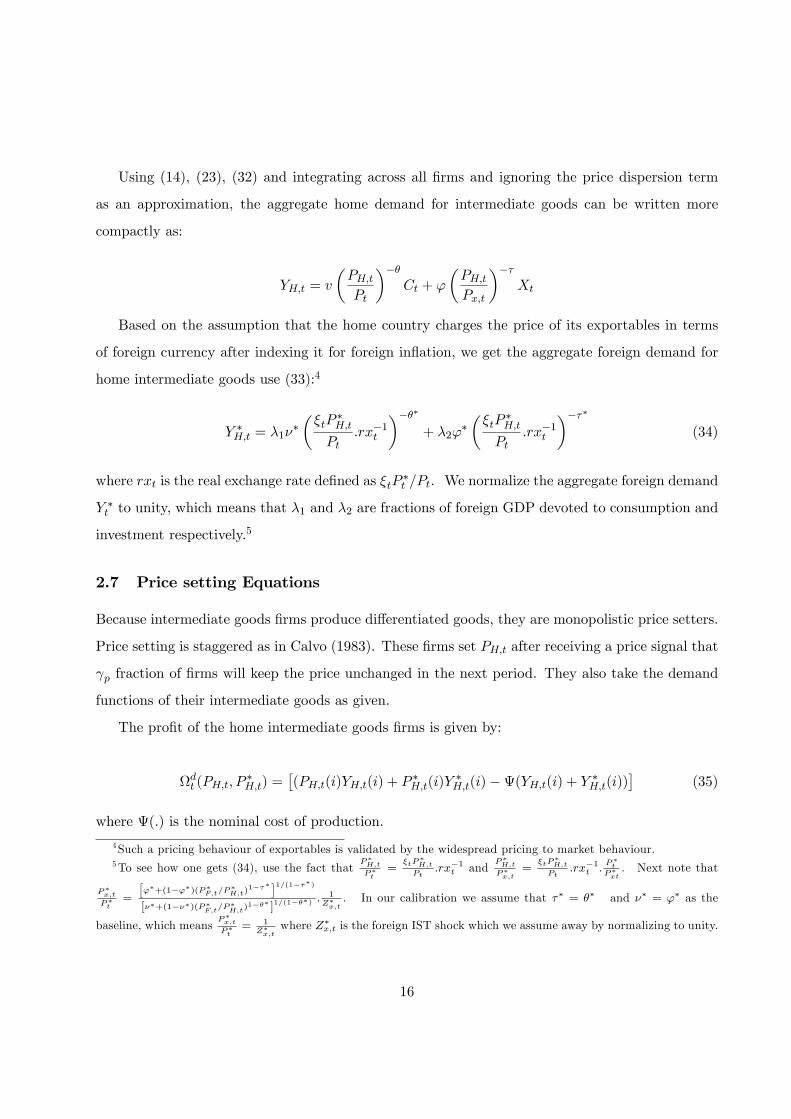
Using (14), (23), (32) and integrating across all firms and ignoring the price dispersion term
as an approximation, the aggregate home demand for intermediate goods can be written more
compactly as:
YH,t = v
(PH,tPt
)−θCt + ϕ
(PH,tPx,t
)−τXt
Based on the assumption that the home country charges the price of its exportables in terms
of foreign currency after indexing it for foreign inflation, we get the aggregate foreign demand for
home intermediate goods use (33):4
Y ∗H,t = λ1ν∗(ξtP
∗H,t
Pt.rx−1t
)−θ∗+ λ2ϕ
∗(ξtP
∗H,t
Pt.rx−1t
)−τ∗(34)
where rxt is the real exchange rate defined as ξtP∗t /Pt. We normalize the aggregate foreign demand
Y ∗t to unity, which means that λ1 and λ2 are fractions of foreign GDP devoted to consumption and
investment respectively.5
2.7 Price setting Equations
Because intermediate goods firms produce differentiated goods, they are monopolistic price setters.
Price setting is staggered as in Calvo (1983). These firms set PH,t after receiving a price signal that
γp fraction of firms will keep the price unchanged in the next period. They also take the demand
functions of their intermediate goods as given.
The profit of the home intermediate goods firms is given by:
Ωdt (PH,t, P
∗H,t) =
[(PH,t(i)YH,t(i) + P ∗H,t(i)Y
∗H,t(i)−Ψ(YH,t(i) + Y ∗H,t(i))
](35)
where Ψ(.) is the nominal cost of production.
4Such a pricing behaviour of exportables is validated by the widespread pricing to market behaviour.5To see how one gets (34), use the fact that
P∗H,tP∗t
=ξtP
∗H,t
Pt.rx−1t and
P∗H,tP∗x,t
=ξtP
∗H,t
Pt.rx−1t .
P∗tP∗xt. Next note that
P∗x,tP∗t
=
[ϕ∗+(1−ϕ∗)(P∗F,t/P
∗H,t)
1−τ∗]1/(1−τ∗)
[ν∗+(1−ν∗)(P∗F,t/P∗H,t
)1−θ∗ ]1/(1−θ∗) .
1Z∗x,t
. In our calibration we assume that τ∗ = θ∗ and ν∗ = ϕ∗ as the
baseline, which meansP∗x,tP∗t
= 1Z∗x,t
where Z∗x,t is the foreign IST shock which we assume away by normalizing to unity.
16
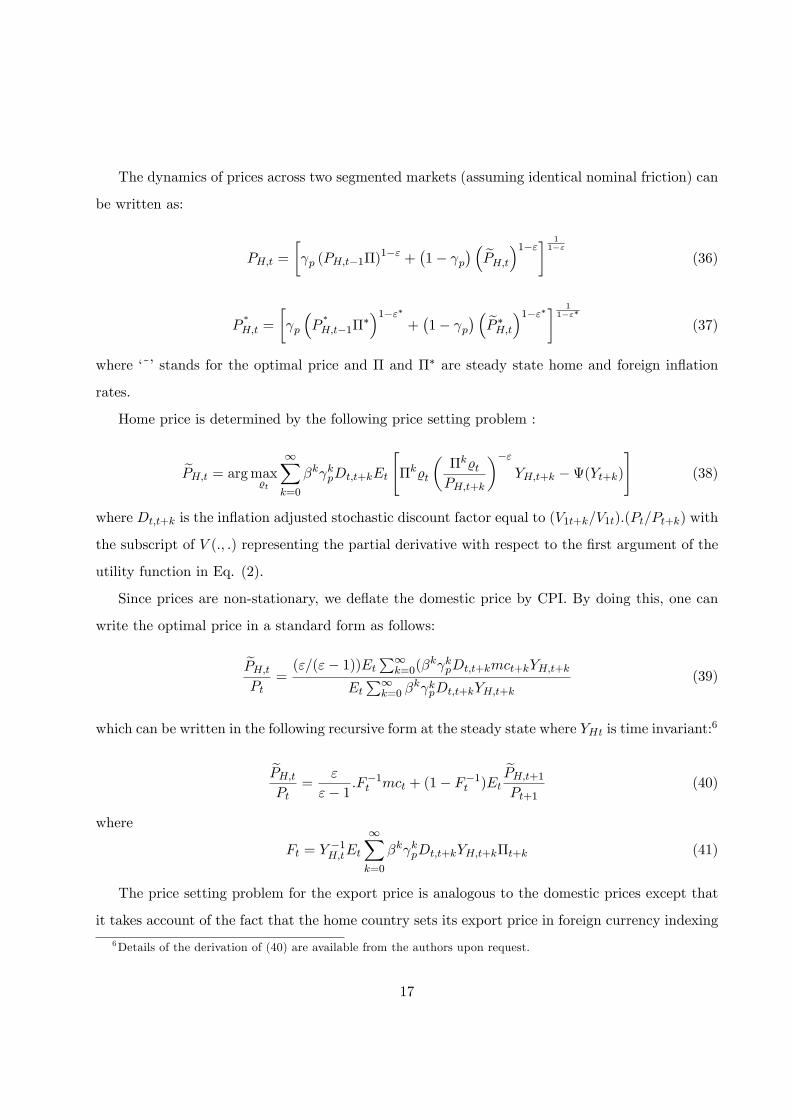
The dynamics of prices across two segmented markets (assuming identical nominal friction) can
be written as:
PH,t =
[γp (PH,t−1Π)1−ε +
(1− γp
) (PH,t
)1−ε] 11−ε
(36)
P∗H,t =
[γp
(P∗H,t−1Π
∗)1−ε∗
+(1− γp
) (P ∗H,t
)1−ε∗] 11−ε∗
(37)
where ‘ ’stands for the optimal price and Π and Π∗ are steady state home and foreign inflation
rates.
Home price is determined by the following price setting problem :
PH,t = arg max%t
∞∑k=0
βkγkpDt,t+kEt
[Πk%t
(Πk%tPH,t+k
)−εYH,t+k −Ψ(Yt+k)
](38)
where Dt,t+k is the inflation adjusted stochastic discount factor equal to (V1t+k/V1t).(Pt/Pt+k) with
the subscript of V (., .) representing the partial derivative with respect to the first argument of the
utility function in Eq. (2).
Since prices are non-stationary, we deflate the domestic price by CPI. By doing this, one can
write the optimal price in a standard form as follows:
PH,tPt
=(ε/(ε− 1))Et
∑∞k=0(β
kγkpDt,t+kmct+kYH,t+k
Et∑∞
k=0 βkγkpDt,t+kYH,t+k
(39)
which can be written in the following recursive form at the steady state where YHt is time invariant:6
PH,tPt
=ε
ε− 1.F−1t mct + (1− F−1t )Et
PH,t+1Pt+1
(40)
where
Ft = Y −1H,tEt
∞∑k=0
βkγkpDt,t+kYH,t+kΠt+k (41)
The price setting problem for the export price is analogous to the domestic prices except that
it takes account of the fact that the home country sets its export price in foreign currency indexing
6Details of the derivation of (40) are available from the authors upon request.
17

it against foreign steady state inflation rate Π∗ as in Kollmann (2002). It is given by:7
P ∗H,t = arg maxκt
∞∑k=0
βkγkpDt,t+kEt
ξt+kΠ∗kκt(κtΠ∗
k
Pt+k
)−ε∗Y ∗H,t+k −Ψ(Yt+k)
(42)
The optimal export price can be written analogously as:8
ξtP∗H,t
Pt=
(ε∗/(ε∗ − 1))Et∑∞
k=0 βkγkpDt,t+kmct+kY
∗H,t+kΠt+k
Et∑∞
k=0(γpΠ∗−ε∗)kDt,t+kY
∗H,t+kΠt+k
(43)
which gives rise to the following recursive representation of the relative export price with respect
to the home CPI:
P ∗H,tξtPt
=ε∗
ε∗ − 1F ∗−1t mct + Π∗ε
∗(1− F ∗−1t )Et
P ∗H,t+1ξt+1Pt+1
(44)
where
F ∗t = Y ∗−1H,t Et
∞∑k=0
βkγkpΠ∗−kε∗Dt,t+kY
∗H,t+kΠt+k (45)
Not surprisingly, the relative domestic and export prices (40) and (44) depend positively on the
current and anticipated real marginal cost via the staggered price setting rules.
2.8 Fiscal Policy
The home government consumes Gt of final consumption goods and finances this by lump sum
taxes Tt and borrowing. The government issues bonds which are domestically held. In other words,
the government budget constraint is:
PtGt − Tt =BHt+11 + it
−BHt (46)
7 In a world of law of one price (LOOP) , the foreign terms of trade is identical to home terms of trade and thus theexport price setting equation becomes redundant. However, we do not assume LOOP in our model as in Kollmann(2002).
8The details of the derivation of (44) are available upon request from the authors.
18
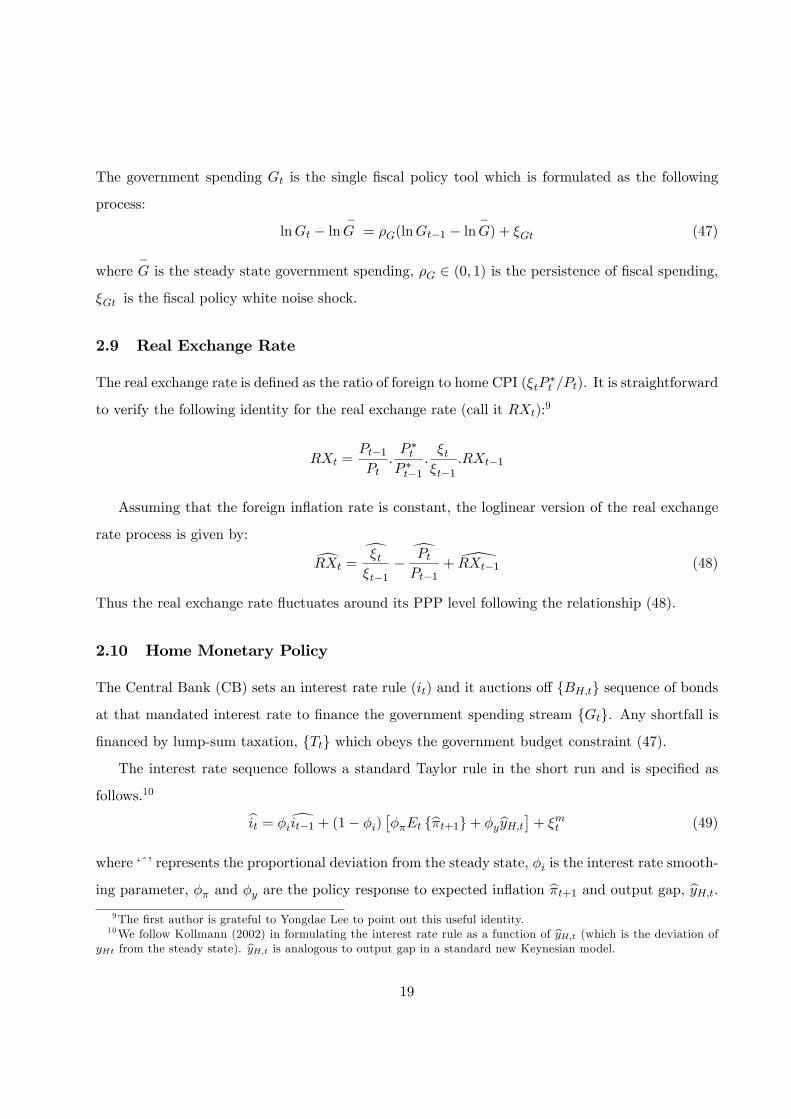
The government spending Gt is the single fiscal policy tool which is formulated as the following
process:
lnGt − ln−G = ρG(lnGt−1 − ln
−G) + ξGt (47)
where−G is the steady state government spending, ρG ∈ (0, 1) is the persistence of fiscal spending,
ξGt is the fiscal policy white noise shock.
2.9 Real Exchange Rate
The real exchange rate is defined as the ratio of foreign to home CPI (ξtP∗t /Pt). It is straightforward
to verify the following identity for the real exchange rate (call it RXt):9
RXt =Pt−1Pt
.P ∗tP ∗t−1
.ξtξt−1
.RXt−1
Assuming that the foreign inflation rate is constant, the loglinear version of the real exchange
rate process is given by:
RXt =ξtξt−1
− PtPt−1
+ RXt−1 (48)
Thus the real exchange rate fluctuates around its PPP level following the relationship (48).
2.10 Home Monetary Policy
The Central Bank (CB) sets an interest rate rule (it) and it auctions off BH,t sequence of bonds
at that mandated interest rate to finance the government spending stream Gt. Any shortfall is
financed by lump-sum taxation, Tt which obeys the government budget constraint (47).
The interest rate sequence follows a standard Taylor rule in the short run and is specified as
follows.10
it = φiit−1 + (1− φi)[φπEt πt+1+ φyyH,t
]+ ξmt (49)
where ‘ ’represents the proportional deviation from the steady state, φi is the interest rate smooth-
ing parameter, φπ and φy are the policy response to expected inflation πt+1 and output gap, yH,t.
9The first author is grateful to Yongdae Lee to point out this useful identity.10We follow Kollmann (2002) in formulating the interest rate rule as a function of yH,t (which is the deviation of
yHt from the steady state). yH,t is analogous to output gap in a standard new Keynesian model.
19

We assume that the home monetary authority is solely concerned about the domestic inflation and
output fluctuations in designing its own monetary policy.11
2.11 Market Equilibrium
The solution to our model satisfies the following market equilibrium conditions must hold for the
home and foreign country:
1. Home-produced intermediate goods market clears:
Yt = YH,t + Y ∗H,t (50)
2. Foreign-produced intermediate goods market clears:
Y ∗t
= YF,t + Y ∗F,t (51)
3. Bond Market clears:
ξtBF,t
Pt(1 + i∗t )Θ(ξtBF,tPt
) − ξtBF,t−1Pt
=ξtP
∗H,t
PtY ∗H,t −
PF,tPt
YFt (52)
4. BHt follows the government budget constraint (46).
Note that the first equality in (52) shows the current account balance. The right hand side is
home country’s net export.
11One may debate whether during the QE phase, the RBI explicitly followed the lead given by the major playersuch as Federal Reserve or ECB in formulating its own monetary policy. There is no clear such evidence that it wasthe case. In fact the data (as seen Figure 2) suggest that the Indian Repo rate diverged from the US Federal Fundsrate since 2009 which is contrary to such posited leader-follower relationship. We thus assume that the home CentralBank basically follows a traditional forward looking Taylor rule.
20

2.12 National Income Accounting
It is straightforward to verify that the Walras law holds for the aggregate economy. Aggregate the
flow budget constraints of all home households to get:
PtCt + Px,tXt +BH,t+1(1 + it)
+ξtBF,t
(1 + i∗t )Θ(ξtBF,tPt
)= BH,t + ξtBF,t−1 +WtLt +Rk,tKt + Ωd
t − Tt
Then substitute the bond market clearing condition (52) to get:
PtCt + Px,tXt +BHt+1(1 + it)
−BHt + P ∗H,tξtY∗H,t − PF,tYF,t = WtLt +Rk,tKt + Ωd
t − Tt (53)
However the aggregate profit is given by:
Ωdt = PH,tYt −WtLt −Rk,tKt (54)
which after plugging into (53) yields
PtCt + PxtXt +BHt+1(1 + it)
−BHt + P ∗H,tξtY∗H,t − PF,t(CF,t +XFt) = PH,tYt − Tt (55)
Finally substitute the government budget constraint to get rid of the tax term yields
PtCt + PxtXt + PtGt + P ∗H,tξtY∗H,t − PF,tYFt = PH,tYt (56)
Note that (P ∗H,tξtY∗H,t−PF,tYFt) is home country’s net export. Thus we verify the national income
identity.
2.13 Modified Uncovered Interest Parity Condition
From (9) and (10),1 + it1 + i∗t
= Etξt+1ξt
.Θ(ξtBFtPt
) (57)
The bond holding cost function Θ(.) drives wedge between home and foreign bond returns.
21

3 Modelling Quantitative Easing
Motivated by a persistent decline in the US federal funds rate during the QE era, we model the
quantitative easing shock as a negative shock in the foreign interest rate with a slow recovery. A
positive eight quarter ahead "news" shock is added to the foreign interest rate to represent the
"taper talk." 12In other words, the foreign interest is modelled as:
i∗t = φ∗i i∗t−1 − (ξ∗mt − ξ∗mt−8) (58)
where φ∗i is the phasing our parameter and ξ∗mt is a white noise. The baseline parameterization of
the model is shown in Table 1. There are four additional shocks in the model namely, TFP (At),
IST (Zxt ), fiscal spending (Gt), and home monetary policy (it). Since the centre of attention in this
paper is the QE shock, we set the serial correlation parameters for all the remaining shocks to zero.
Most of the baseline parameters are close to the values chosen in Banerjee and Basu (2015). We
assume a higher home bias in investment than consumption on par with Banerjee and Basu (2015).
The rationale for choosing a low value for the nominal rigidity parameter γp in the context of India
is also explained in Banerjee and Basu (2015). The steady state inflation rates for home and foreign
countries are fixed at 3% to 2% respectively which means a steady state depreciation rate of 1% for
the home currency.13 The phasing out parameter φ∗i is fixed at 0.86 based on an AR(1) estimation
of the historical annual federal funds rate for the period 1956-2012. The risk aversion parameter σc
is fixed at 2 which is in line with the estimate of Levine and Pearlman(2011). There is no readily
available estimate of the proportion of rule-of-thumb consumers (1 − λ) for the Indian economy.
Gali et al. (2005) use λ = 0.5. Given the existence of a vast informal sector in India, we set a
greater value of 1-λ equal to 0.7. Changing λ in this vicinity has nearly no effect on the impulse
response analysis that we report later.
12An eight quarter lag is arbitrarily chosen assuming that the market foresees the tapering of QE about two yearsahead. Changing this lag to four quarters makes no difference to the impulse response analysis except that the actualtaper materializes after four quarters instead of eight quarters.13Setting a higher steady state inflation rate for the home country does not change the impulse response properties
of the model.
22

Table 1: Baseline Parameterizationβ σc σL γc γp ε ε∗ θ ν ϕ ν∗ ϕ∗ τ α
0.98 2 0 0.6 0.22 6 6 2 0.7 0.8 0.8 0.8 2 0.3
Table 2: Baseline Parameterization (Contd)
δ S”(1) φi φπ φy φ∗i Θ′(−bf ).
−c λ1 λ2 Π Π∗
0.1 2.5 0.81 1.64 0.5 0.86 0.001 0.67 0.24 1.03 1.02
Figure 3 plots the impulse responses of the relevant macroeconomic aggregates followed by one
standard deviation negative shock in the foreign interest rate from a steady state value. This
decline in foreign interest rate is motivated by the sharp drop in the US federal funds rate from
its baseline value of 5% since 2007 (Figure 2). Given the domestic interest rate, such a decline
in foreign interest rate makes the home currency depreciate via the UIP condition (57). Since
home producers of intermediate goods set the export price in foreign currency, the depreciation of
home currency raises the optimal relative price of exportables (P ∗H,tξt/Pt) in (44). Intermediate
goods producers, therefore, experience a rise in export revenue from the sale of intermediate goods
abroad. This encourages them to expand the intermediate goods output for the export market. The
immediate effect of this output expansion is a rise in the real marginal cost mct in eq (44) which in
turn boosts the optimal relative home price of tradeable (PH,t/Pt ) via the price setting rule (40).
This rise in PH,t/Pt fuels domestic inflation via the price aggregator (36). The home Central Bank
reacts to it by raising the nominal interest rate based on the Taylor rule (49). Thus home interest
rate moves in the opposite direction to the change in the foreign rate which is consistent with the
stylized facts reported earlier.
23

0 20 40210
i*
0 20 400
0.05Exchange rate
0 20 400.05
00.05
yh
0 20 400
0.010.02
mc
0 20 400
0.010.02Optimal ξPh*/P
0 20 400
0.010.02
Optimal Ph/P
0 20 400.040.02
0Pf/Ph
0 20 400.05
00.05
GDP
0 20 40024
x 103Px/P
0 20 400
0.05Inflation
0 20 400.05
00.05
i
0 20 400.2
00.2
NX
0 20 400.01
00.01
q
0 20 400
0.010.02
C
0 20 400.05
00.05
X
0 20 400.05
00.05
L
0 20 400.02
00.02
K
0 20 400.0050.01
0.015w
0 20 400.02
00.02
rk
0 20 400.2
00.2
RX
Figure 3: Effect of a QE Shock
Higher real marginal cost translates into a higher real wage and rental price of capital via (31).
Agents respond to this by supply more labour and investing more in physical capital which raises
the Tobin’s q. Higher wage and rental income create positive income effect which boosts household
consumption. The overall impact effect of a QE on GDP is positive which reflects the spurt in
home intermediate goods production but it is rather small because of the decline in net export.
3.1 Effect of a QE Taper Talk
Figure 2 plots the impulse response of a "news" that QE will be phased out. We model this as
an expected rise in foreign interest rate eight quarters ahead which means a positive shock to
ξt−8. Market anticipates an appreciation of home currency which translates into a lower expected
relative price of exportable via the price setting function. The real effect of such taper talk works
opposite to the effect a negative QE shock discussed in the earlier section. Intermediate goods
producers react to this news about QE phase out by cutting back tradeable intermediate goods
24

production (YHt). This lowers the real marginal cost, mc and it then translates into a lower inflation
immediately via the price aggregator. The CB lowers interest rate in response to low inflation via
the Taylor rule before the exchange rate actually appreciates. The anticipation of appreciation of
home currency becomes a reality after eight quarters via the uncovered interest parity condition.
However, following this monetary appreciation episode, home currency depreciates again as foreign
interest rate reverts to its mean.
Given that the nominal exchange rate is not altered for eight quarters, lower domestic inflation
raises the real exchange rate (RX) which translates into a higher optimal export price (ξtP∗Ht/Pt).
This boosts the real marginal cost and it raises PH/P. The terms of trade PF /PH moves in the
opposite direction to PH/P following the price aggregator (26). Higher relative price of home goods
shows up as an increase in GDP (see eq. 56)). The current account shows swings in response to this
news effect due to conflicting movement of different relative prices. Not surprisingly, the Tobin’s q
mimics the pattern of the real marginal cost. The rest of the effects are similar as before.
The bottom-line of this impulse responses to QE taper news is that there are sudden reversal in
the behaviour of some key macroeconomic aggregates such as the nominal exchange rate, net export
and Tobin’s q due to the expectations effect. For example, the terms of trade initially declines but
then as soon as the tapering is realized after eight quarters, it reverses its course. The same also
happens for the CPI inflation. There is initial deflation and then inflation picks up its momentum.
The financial market summarized by the Tobin’s q shows similar reversal.. Taper talk thus possibly
gives rise to more volatility in these key macroeconomic aggregates.14
14We use the term volatility in the sense of sudden change in the track. Evidently, we are not addressing issueof volatility spillover which requires serious modelling of the second order effects of QE shocks. This is beyond thescope of this paper.
25

0 20 40101
i*
0 20 400.05
00.05
Exchange rate
0 20 400.05
00.05
yh
0 20 400.01
00.01
mc
0 20 400.01
00.01
Optimal ξPh*/P
0 20 400.01
00.01
Optimal Ph/P
0 20 400.05
00.05
Pf/Ph
0 20 400.05
00.05
GDP
0 20 40505
x 103Px/P
0 20 400.1
00.1
Inflation
0 20 400.05
00.05
i
0 20 400.2
00.2
NX
0 20 400.01
00.01
q
0 20 400.01
00.01
C
0 20 400.05
00.05
X
0 20 400.05
00.05
L
0 20 400.05
00.05
K
0 20 400.01
00.01
w
0 20 400.02
00.02
rk
0 20 400.2
00.2
RX
Figure 4: Effect of a QE Taper Talk
4 Conclusion
The aim of this paper is to develop a stylized DSGE framework to understand the effect of QE in
a small open economy like India. This exercise is motivated by some broad stylized facts about the
behaviour of key macroeconomic aggregates. What is novel in this paper is to highlight the effect of
QE on the macroeconomy via the external terms of trade channel. Our model predicts that the QE
innovation raises the real marginal cost of production in the home country because intermediate
goods producers experience a favourable terms of trade effect and step up their production. This
higher real marginal cost translates into inflation through the standard new Keynesian Phillips curve
channel. The home Central Bank raises interest rate to respond to this inflation which explains the
pervasive stylized fact that the home and foreign interest rates move in opposite directions after a
few periods of QE innovation. We also model the QE taper talk as a "news" about future increase
in foreign interest rate. Such a news effect creates market expectation about future appreciation of
26
home nominal interest rate which impacts the terms of trade positively as observed in the data. Our
DSGE model predicts that such "news" would give rise to greater volatility in key macroeconomic
aggregates in terms of a sudden change in their time paths.
The issue still remains whether the QE had any real macroeconomic effects on the Indian
economy. Our impulse response analysis suggests that the effect of QE shock in the real GDP
is rather minimal. It is still diffi cult to draw any definitive conclusion from the present model
due to its highly stylized nature and the non-availability of high frequency data for real economic
aggregates. In a companion paper (Banerjeee and Basu, 2015) we find that the aggregate effect
of foreign interest rate shock is minimal and the aggregate fluctuations are more governed by the
investment specific technology shocks during the post liberalization period. Our present model also
abstracts from many complications such as tax distortions, informal labour market, banking and
credit market frictions. We also believe that banking frictions as in Gertler and Karadi (2012)
are less important for India because of its highly regulated banking industry and this is why we
assumed it away in our model. Credit market frictions in terms of a lending-borrowing spread
and informal labour market can be introduced but it is unlikely to alter the main punchline of the
paper.
27

References
[1] Abel, A. B.(1990) "Asset Prices under Habit Formation and Catching up with the Joneses"
American Economic Review, Vol. 80, No. 2, May.
[2] Anand, Rahul, and Peiris, Shanaka, and Saxegaard, Magnus (2010) "An Estimated Model
with Macrofinancial Linkages for India", IMF Working Paper Series, WP/10/21.
[3] Banerjee S and P Basu (2014) "A Dynamic Stochastic General Equilibrium Model for India,"
working paper no 109, NCAER.
[4] Banerjee S and P Basu (2015) "Technology Shocks and Business Cycles in India: Role of Home
Bias in Consumption," working paper.
[5] Backus, D., Kehoe, P. and Kydland, F. (1994) "Dynamics of the trade balance and the terms
of trade: the J -curve" American Economic Review 84, pp 84-103.
[6] Barroso, J., Pereira Da Silva, L., Sales, A. (2013) "Quantitative easing and related capital flows
into Brazil: Measuring its effects and transmission channels through a rigorous counterfactual
evaluation. Banco Central Do Brasil", Working Paper Series 313, July.
[7] Basu, K., Eichengreen, B., and Gupta, P.(2014) "From Tapering to Tightening: The Impact
of the Fed’s Exit on India", India Policy Forum
[8] Basu, P and C. Thoenissen (2011) "International Business Cycles and the Relative Price of
Investment", Canadian Journal of Economics, (2011), 44, 2. pp 586-606
[9] Benigno, P. (2009). Price stability with imperfect financial integration. Journal of Money,
Credit and Banking, Vol. 41, Issue s1, pp. 121 —149, (2009).
[10] Bhattacharya Rudrani and Patnaik Ila (2013) Credit constraints, productivity shocks and
consumption volatility in emerging economies," IMF Working Paper No. WP/13/120.
[11] Christiano, Lawrence J., Eichenbaum, Martin and Evans, Charles L. (2005) "Nominal Rigidi-
ties and the Dynamic Effects of a Shock to Monetary Policy," Journal of Political Economy,
University of Chicago Press, University of Chicago Press, vol. 113(1), pages 1-45, February.
28

[12] Eichengreen, B., and Gupta, P., 2014. Tapering talk: The impact of expectations of reduced
Federal Reserve security purchases on Emerging Markets. Policy Research Working Paper
Series 6754, The World Bank.
[13] Gali, J, J.D. Lopez-Salido and J. Valles (2005), "Understanding the Effects of Government
Spending on Consumption," working paper.
[14] Gertler, M and P. Karadi (2011), "A model of unconventional monetray policy" Journal of
Monetary Economics, 56, pp. 17-34.
[15] Heathcote, J. and Perri, F. (2002). Financial autrarky and international business cycles. Jour-
nal of Monetary Economics, vol. 49, pp 601-27.
[16] Hodrick, R J. & Prescott, E.C., (1997). "Postwar U.S. Business Cycles: An Empirical Investi-
gation," Journal of Money, Credit and Banking, Blackwell Publishing, vol. 29(1), pages 1-16,
February.
[17] Kollmann, R (2002), Monetary Policy Rules in the Open Economy: Effects on Welfare and
Business Cycles, Journal of Monetary Economics, pp 989-1015.
[18] Lavigne, R., Sarker, S., and Vasishtha, G., 2014. Spillover effects of quantitative easing on
Emerging Market Economies. Bank of Canada Review, Autumn.
[19] Levine, Paul and Pearlman, Joseph (2011). “Monetary and Fiscal Policy in a DSGE Model of
India”, Working Papers, National Institute of Public Finance and Policy, 11/96.
[20] Mishra, P., Moriyama, K., N’Diaye, P., and Nguyen, L., 2014. Impact of Fed Tapering an-
nouncements on Emerging Markets. International Monetary Fund Working Paper, June.
[21] Parente, S and E.C. Prescott, Barriers to Riches, MIT Press, August 2000.
[22] Rai, V., and Suchanek, L., 2014. The effect of the Federal Reserve’s tapering announcements
on Emerging Markets, Bank of Canada Working Paper 2014-50, November.
29

[23] Rajan, R. G., (2014). Concerns about Competitive Monetary Easing, Policy Panel Discussion,
Conference on Monetary Policy in a Post-Financial Crisis Era, Institute of Monetary and
Economic Studies, Bank of Japan in Tokyo on May 28, 2014.
[24] Tillmann, P., 2014. Unconventional monetary policy shocks and the spillovers to Emerging
Markets, Honkong Institute for Monetary Research Working Paper 18/2014, August.
30