EECS730: Introduction to Bioinformatics

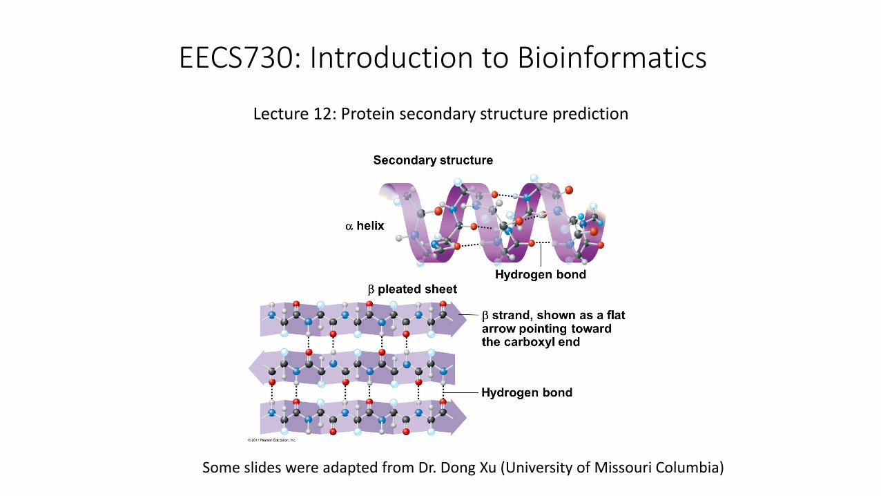
Lecture 12: Protein secondary structure prediction

Some slides were adapted from Dr. Dong Xu (University of Missouri Columbia)

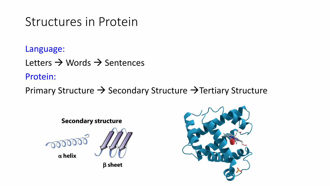
Structures in Protein

Language:

Letters Words Sentences

Protein:

Primary Structure Secondary Structure Tertiary Structure

Protein side chains

https://s-media-cache-ak0.pinimg.com/originals/ed/c0/ca/edc0ca6e8323df7bce06fd72ab5eca80.gif

a helix

Single protein chain (local)

Shape maintained byintramolecular H bondingbetween -C=O and H-N-

b sheet

Several protein chains

Shape maintained byintramolecular H bondingbetween chains

Non-local on protein sequence

b -sheet (parallel, anti-parallel)

Random coil

“A random coil is a polymer conformation where the monomer subunits are oriented randomly while still being bonded to adjacent units.” - Wikipedia

http://www.pnas.org/content/101/34/12497/F3.large.jpghttps://getrevising.co.uk/revision-cards/biology_asf212ocr_specification_and_answers

Classification of secondary structure

• Defining features• Dihedral angles

• Hydrogen bonds

• Geometry

• Assigned manually by experimentalists

• Automatic• DSSP (Kabsch & Sander,1983)

• STRIDE (Frishman & Argos, 1995)

• Continuum (Andersen et al.)

Classification

• Eight states from DSSP H: a-helix

G: 310 helix

I: p-helix

E: b-strand

B: bridge

T: b-turn

S: bend

C: coil

• CASP Standard H = (H, G, I), E = (E, B), C = (C, T, S)

24 26 E H < S+ 0 0 132

25 27 R H < S+ 0 0 125

26 28 N < 0 0 41

27 29 K 0 0 197

28 ! 0 0 0

29 34 C 0 0 73

30 35 I E -cd 58 89B 9

31 36 L E -cd 59 90B 2

32 37 V E -cd 60 91B 0

33 38 G E -cd 61 92B 0

Dihedral angles

Ramachandran plot (alpha)

Ramachandran plot (beta)

Protein secondary structure prediction

Given a protein sequence (primary structure)

GHWIATRGQLIREAYEDYRHFSSECPFIP

Predict its secondary structure content

(C=Coils H=Alpha Helix E=Beta Strands)

CEEEEECHHHHHHHHHHHCCCHHCCCCCC

Protein secondary structure prediction

• An easier problem than 3D structure prediction (more than 40 years of history).

• Accurate secondary structure prediction can be an important information for the tertiary structure prediction

• Protein function prediction

• Protein classification

• Predicting structural change

Naïve way

• You can always predict protein secondary structure by pairwise sequence alignment

• Similar to the non-coding RNA sequence-structure alignment

• We are going to focus on scenarios where no homology can be detected (no good alignment can be computed)

• De novo prediction

Summary of methods

Statistical methodChou-Fasman method, GOR I-IV

Nearest neighborsNNSSP, SSPAL

Neural networkPHD, Psi-Pred, J-Pred

Support vector machine (SVM)

HMM

Measure

Three-state prediction accuracy: Q3

correctly predicted residues

number of residues3Q

A prediction of all loop: Q3 ~ 40%

Accuracy

1974 Chou & Fasman ~50-53%1978 Garnier 63%1987 Zvelebil 66%1988 Qian & Sejnowski 64.3%1993 Rost & Sander 70.8-72.0%1997 Frishman & Argos <75%1999 Cuff & Barton 72.9%1999 Jones 76.5%2000 Petersen et al. 77.9%

0

5

10

15

20

25

30 40 50 60 70 80 90 100

PSIPRED

SSpro

PROF

PHDpsi

JPred2

PHD

Perc

enta

ge o

f al

l 15

0 pr

otei

ns

Percentage correctly predicted residues per protein

Assumptions

• The entire information for forming secondary structure is contained in the primary sequence.

• Side groups of residues will determine structure.

• Examining windows of 13 - 17 residues is sufficient to predict structure.

• Basis for window size selection:

• a-helices 5 – 40 residues long

• b-strands 5 – 10 residues long

Chou-Fasman Method

From PDB database, calculate the propensity for a

given amino acid to adopt a certain ss-type

( | ) ( , )

( ) ( ) ( )

i i i

i

P aa p aaP

p p p aaa

a a

a a

Example:

#Ala=2,000, #residues=20,000, #helix=4,000, #Ala in helix=500

P(a,aai) = 500/20,000, p(a) 4,000/20,000, p(aai) = 2,000/20,000

P = 500 / (4,000/10) = 1.25

Chou-Fasman Method

Chou-Fasman Method

Helix, Strand1. Scan for window of 6 residues where average score > 1 (4 residues

for helix and 3 residues for strand)

2. Propagate in both directions until 4 (or 3) residue window with mean propensity < 1

3. Move forward and repeat

Conflict solutionAny region containing overlapping alpha-helical and beta-strand assignments are taken to be helical if the average P(helix) > P(strand). It is a beta strand if the average P(strand) > P(helix).

Accuracy: ~50% ~60%

GHWIATRGQLIREAYEDYRHFSSECPFIP

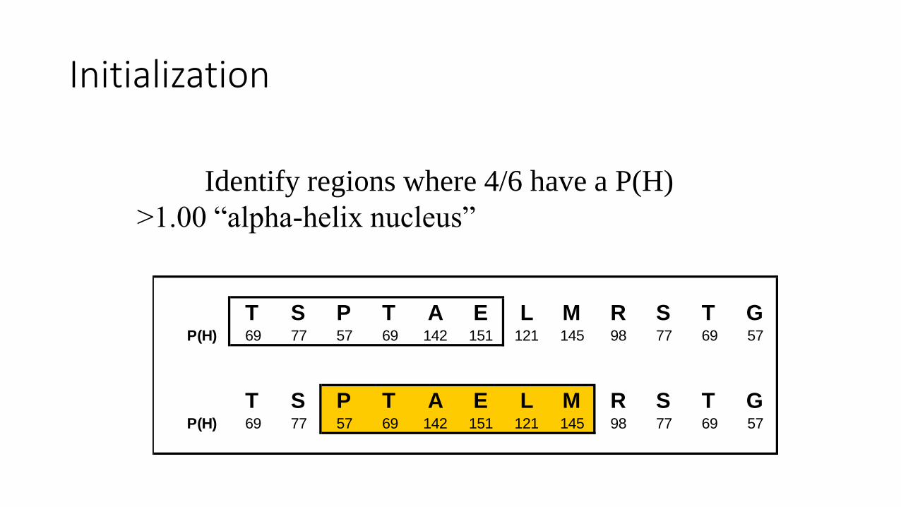
Initialization

T S P T A E L M R S T GP(H) 69 77 57 69 142 151 121 145 98 77 69 57

T S P T A E L M R S T GP(H) 69 77 57 69 142 151 121 145 98 77 69 57

Identify regions where 4/6 have a P(H)

>1.00 “alpha-helix nucleus”

Extension

T S P T A E L M R S T GP(H) 69 77 57 69 142 151 121 145 98 77 69 57

Extend helix in both directions until a set

of four residues have an average P(H) <1.00.

Nearest Neighbor Method

o Predict secondary structure of the central residue of a given segment from homologous segments (neighbors)

(i) From database, find some number of the closest sequences to a subsequence defined by a window around the central residue

(ii) Compute K best non-intersecting local alignments of a query sequence with each sequence.

o Use max (na, nb, nc) for neighbor consensus or max(sa, sb, sc) for consensus sequence hits

Environment preference score

Each amino acid has a preference to a specific structural environments.

Structural variables:

secondary structure, solvent accessibility

Non-redundant protein structure database: FSSP

( | ) ( , )( , ) log log

( ) ( ) ( )

i j i j

i i j

p aa E p aa ES i j

p aa p aa p E

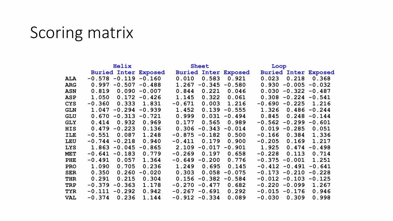
Scoring matrix

Helix Sheet LoopBuried Inter Exposed Buried Inter Exposed Buried Inter Exposed

ALA -0.578 -0.119 -0.160 0.010 0.583 0.921 0.023 0.218 0.368ARG 0.997 -0.507 -0.488 1.267 -0.345 -0.580 0.930 -0.005 -0.032ASN 0.819 0.090 -0.007 0.844 0.221 0.046 0.030 -0.322 -0.487ASP 1.050 0.172 -0.426 1.145 0.322 0.061 0.308 -0.224 -0.541CYS -0.360 0.333 1.831 -0.671 0.003 1.216 -0.690 -0.225 1.216GLN 1.047 -0.294 -0.939 1.452 0.139 -0.555 1.326 0.486 -0.244GLU 0.670 -0.313 -0.721 0.999 0.031 -0.494 0.845 0.248 -0.144GLY 0.414 0.932 0.969 0.177 0.565 0.989 -0.562 -0.299 -0.601HIS 0.479 -0.223 0.136 0.306 -0.343 -0.014 0.019 -0.285 0.051ILE -0.551 0.087 1.248 -0.875 -0.182 0.500 -0.166 0.384 1.336LEU -0.744 -0.218 0.940 -0.411 0.179 0.900 -0.205 0.169 1.217LYS 1.863 -0.045 -0.865 2.109 -0.017 -0.901 1.925 0.474 -0.498MET -0.641 -0.183 0.779 -0.269 0.197 0.658 -0.228 0.113 0.714PHE -0.491 0.057 1.364 -0.649 -0.200 0.776 -0.375 -0.001 1.251PRO 1.090 0.705 0.236 1.249 0.695 0.145 -0.412 -0.491 -0.641SER 0.350 0.260 -0.020 0.303 0.058 -0.075 -0.173 -0.210 -0.228THR 0.291 0.215 0.304 0.156 -0.382 -0.584 -0.012 -0.103 -0.125TRP -0.379 -0.363 1.178 -0.270 -0.477 0.682 -0.220 -0.099 1.267TYR -0.111 -0.292 0.942 -0.267 -0.691 0.292 -0.015 -0.176 0.946VAL -0.374 0.236 1.144 -0.912 -0.334 0.089 -0.030 0.309 0.998

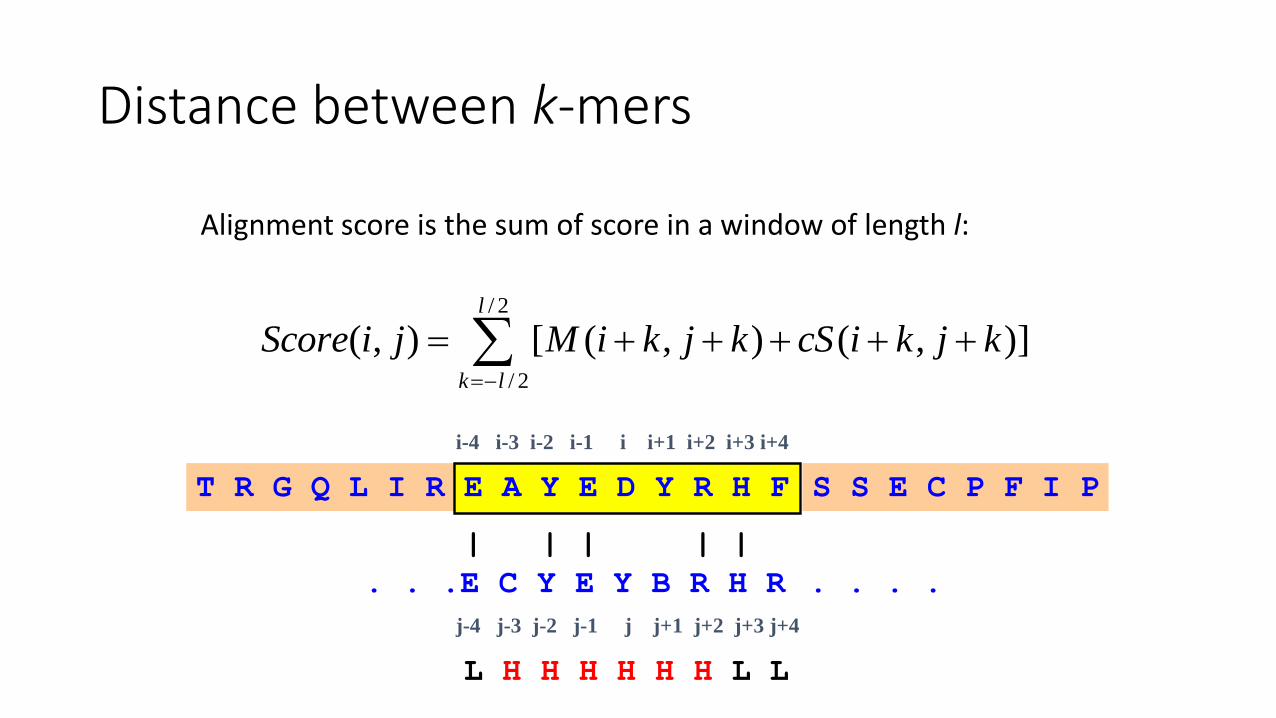
Distance between k-mers

Alignment score is the sum of score in a window of length l:

/ 2

/ 2

( , ) [ ( , ) ( , )]l

k l

Score i j M i k j k cS i k j k-

T R G Q L I R

i-4 i-3 i-2 i-1 i i+1 i+2 i+3 i+4

E A Y E D Y R H F S S E C P F I P

. . .E C Y E Y B R H R . . . .

j-4 j-3 j-2 j-1 j j+1 j+2 j+3 j+4

| | | | |

L H H H H H H L L

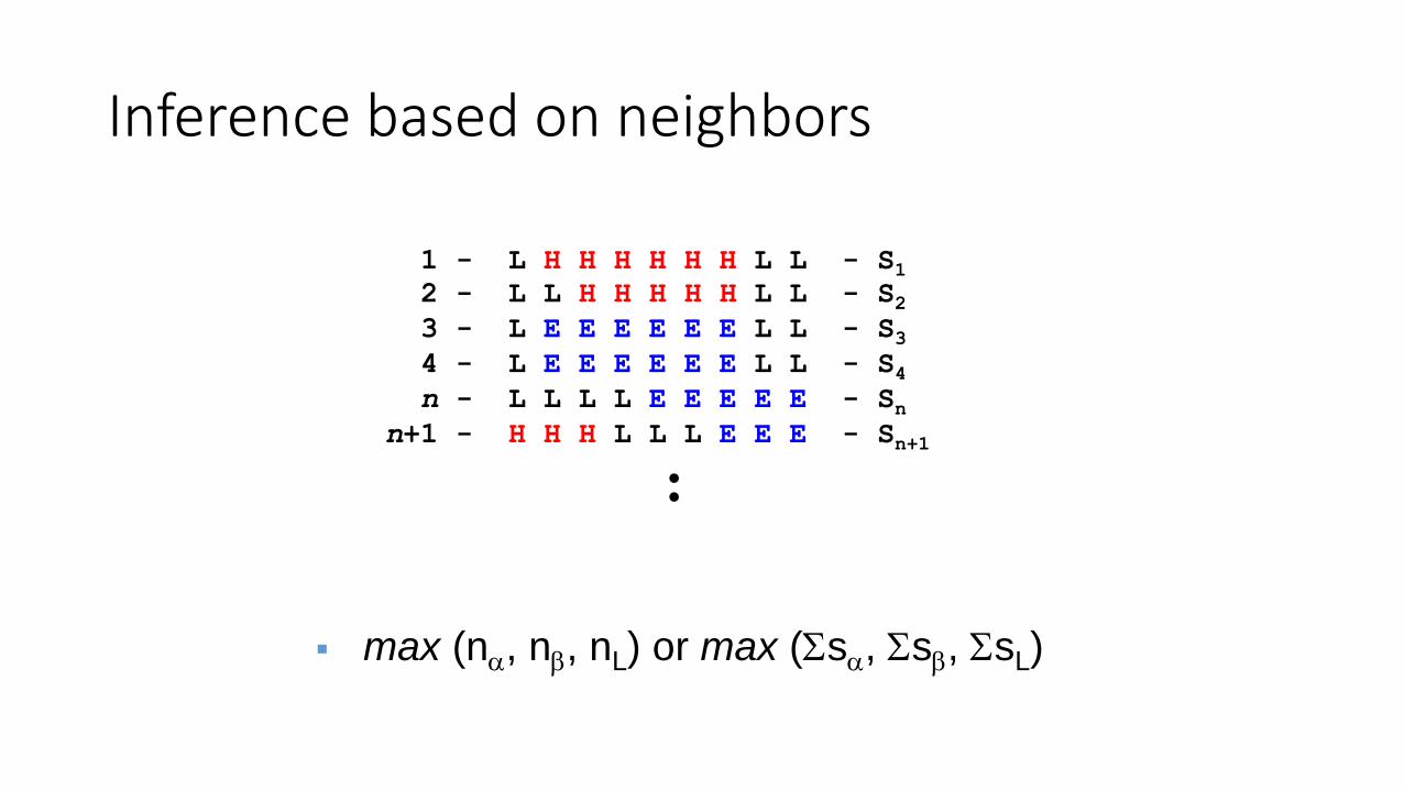
Inference based on neighbors

1 - L H H H H H H L L - S12 - L L H H H H H L L - S23 - L E E E E E E L L - S34 - L E E E E E E L L - S4n - L L L L E E E E E - Sn

n+1 - H H H L L L E E E - Sn+1

:

max (na, nb, nL) or max (Ssa, Ssb, SsL)

Incorporating evolutionary information

“All naturally evolved proteins with more than 35% pairwise identical residues over more than 100 aligned residues have similar structures.”

Stability of structure w.r.t. sequence divergence (<12% difference in secondary structure).

Position-specific sequence profile, containing crucial information on evolution of protein family, can help secondary structure prediction (increase information content).

Gaps rarely occur in helix and strand.

~1.4%/year increase in Q3 due to database growth at the beginning.

Evolution information

Sequence-profile alignment.

Compare a sequence against protein family.

More specific.

BLAST vs. PSI-BLAST.

Look up PSSM instead of PAM or BLOSUM.

/ 2

/ 2

( , ) [ ( , ) ( , )]l

k l

Score i j PSSM j k i k cS i k j k-

Achieved accuracy ~75%

PSIPRED (Neuron networks)

D. Jones, J. Mol. Boil. 292, 195 (1999).

Method : Neural network

Input data : PSSM generated by PSI-BLAST

Bigger and better sequence database

Combining several database and data filtering

Training and test sets preparation

No sequence & structural homologues between training and test sets by PSI-BLAST (mimicking realistic situation).

PSIPRED

• PSI-BLAST (iterative sequence-profile alignment)

• Searching the target sequencing against protein database and generates profile

• The profile contains evolutionary information

• Use profile of proteins with known secondary structure as training for neuron network

PSIPRED

• A window of 15 amino acid residues was found to be optimal.

• The first input layer comprises 315 input units, divided into 15 groups of 21 units. The extra unit per amino acid is used to indicate where the window spans either the N or C terminus of the protein chain.

• A large hidden layer of 75 units was used for the first network, with another three units making the output layer where the units represent the three-states of secondary structure (helix, strand or coil).

• A second network has an input layer comprising just 60 input units, divided into 15 groups of four. Again the extra input in each group is used to indicate that the window spans a chain terminus.

• A smaller hidden layer of 60 units was used for the second network.

PSIPRED

Window size = 15

Two networks

Accuracy ~76%

D. Jones, J. Mol. Boil. 292, 195 (1999).

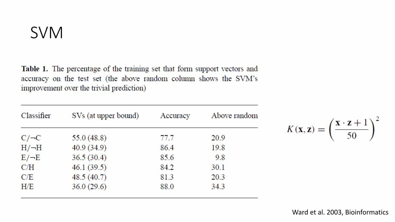
SVM

Ward et al. 2003, Bioinformatics

SVM

• The inputs from each sequence appear in the form of a 20 ×M position-specific scoring matrix from three iterations of a PSI-BLAST search, where M is the length of the target sequence. The scoring matrix for a window of 15 positions, centered on the target residue, is used as the input to the SVM.

• In cases where the window extends beyond the protein termini, ‘empty’ attributes are filled with zeros

Ward et al. 2003, Bioinformatics

SVM cont.

Ward et al. 2003, Bioinformatics

Performance ~77%

Sequence features other than PSSM

Atchley et al., 2005, PNAS

Deep learning network

Spencer et al. 2015, ACM TCBB

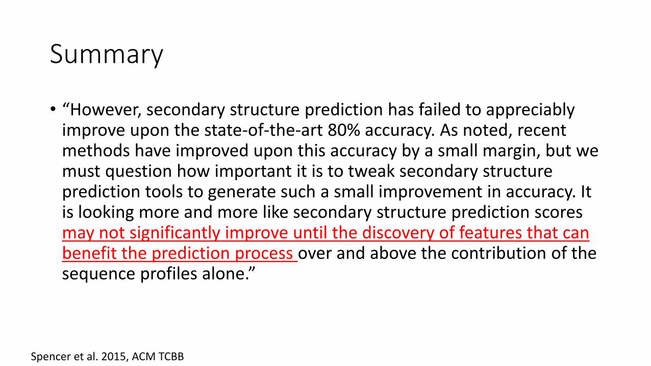
Summary

• “However, secondary structure prediction has failed to appreciably improve upon the state-of-the-art 80% accuracy. As noted, recent methods have improved upon this accuracy by a small margin, but we must question how important it is to tweak secondary structure prediction tools to generate such a small improvement in accuracy. It is looking more and more like secondary structure prediction scores may not significantly improve until the discovery of features that can benefit the prediction process over and above the contribution of the sequence profiles alone.”

Spencer et al. 2015, ACM TCBB