eecs 555: digital communication theory · 2005-01-04 · 1-2 chapter1. introduction 1....
TRANSCRIPT

EECS 555: Digital Communication Theory
Wayne E. Stark
Copyright c�
Wayne E. Stark, 2005

0-2
Contents
1 Introduction 1-11. Communication System Coat of Arms . . . . . . . . . . . . . . . . . . . . . . . . . . . . . . . . 1-2
2 Optimum Receiver Principles 2-11. Detection Theory . . . . . . . . . . . . . . . . . . . . . . . . . . . . . . . . . . . . . . . . . . . 2-1
1. Binary Detection . . . . . . . . . . . . . . . . . . . . . . . . . . . . . . . . . . . . . . . 2-12. Sufficient Statistic . . . . . . . . . . . . . . . . . . . . . . . . . . . . . . . . . . . . . . 2-53. M-ary Detection Problem . . . . . . . . . . . . . . . . . . . . . . . . . . . . . . . . . . 2-6
2. Likelihood Ratio for Random Processes . . . . . . . . . . . . . . . . . . . . . . . . . . . . . . . 2-71. Example . . . . . . . . . . . . . . . . . . . . . . . . . . . . . . . . . . . . . . . . . . . 2-7
3. Detection with Unwanted Parameters . . . . . . . . . . . . . . . . . . . . . . . . . . . . . . . . . 2-104. Likelihood Ratio for Real Signals . . . . . . . . . . . . . . . . . . . . . . . . . . . . . . . . . . 2-115. Likelihood Ratio for Complex Signals . . . . . . . . . . . . . . . . . . . . . . . . . . . . . . . . 2-146. Example: M orthogonal signals in additive white Gaussian noise . . . . . . . . . . . . . . . . . . 2-157. Problems . . . . . . . . . . . . . . . . . . . . . . . . . . . . . . . . . . . . . . . . . . . . . . . 2-16
3 Error Probability for M Signals 3-11. Error Probability for Orthogonal Signals . . . . . . . . . . . . . . . . . . . . . . . . . . . . . . . 3-22. Gallager Bound . . . . . . . . . . . . . . . . . . . . . . . . . . . . . . . . . . . . . . . . . . . . 3-4
1. Example of Gallager bound for M-ary orthogonal signals in AWGN. . . . . . . . . . . . . 3-53. Bit error probability . . . . . . . . . . . . . . . . . . . . . . . . . . . . . . . . . . . . . . . . . . 3-74. Union Bound . . . . . . . . . . . . . . . . . . . . . . . . . . . . . . . . . . . . . . . . . . . . . 3-85. Random Coding . . . . . . . . . . . . . . . . . . . . . . . . . . . . . . . . . . . . . . . . . . . . 3-10
1. Example of Gallager bound for M-ary signals in AWGN. . . . . . . . . . . . . . . . . . . 3-146. Problems . . . . . . . . . . . . . . . . . . . . . . . . . . . . . . . . . . . . . . . . . . . . . . . 3-15
4 Asymptotic Performance 4-11. Capacity Theorem . . . . . . . . . . . . . . . . . . . . . . . . . . . . . . . . . . . . . . . . . . . 4-12. Capacity of Discrete Memoryless Channels: . . . . . . . . . . . . . . . . . . . . . . . . . . . . . 4-153. Summary of Channel Models, Capacity and Cutoff Rate . . . . . . . . . . . . . . . . . . . . . . 4-17
1. Capacity of nonwhite channels . . . . . . . . . . . . . . . . . . . . . . . . . . . . . . . . 4-182. Comments . . . . . . . . . . . . . . . . . . . . . . . . . . . . . . . . . . . . . . . . . . 4-20
4. Bandwidth, Time and Dimensionality . . . . . . . . . . . . . . . . . . . . . . . . . . . . . . . . 4-215. Fundamental limits with nonzero error probability . . . . . . . . . . . . . . . . . . . . . . . . . . 4-216. Problems . . . . . . . . . . . . . . . . . . . . . . . . . . . . . . . . . . . . . . . . . . . . . . . 4-22
5 Noncoherent Receivers 5-11. Optimal Receiver in AGN . . . . . . . . . . . . . . . . . . . . . . . . . . . . . . . . . . . . . . . 5-12. Performance of Binary Signals in AWGN . . . . . . . . . . . . . . . . . . . . . . . . . . . . . . 5-43. Error Probability for M-orthogonal Signals in AWGN . . . . . . . . . . . . . . . . . . . . . . . . 5-64. Error Estimates for Repetition Codes with Noncoherent Reception . . . . . . . . . . . . . . . . . 5-95. Primer on sums of squares of Gaussian random variables . . . . . . . . . . . . . . . . . . . . . . 5-12
0-3

0-4 CONTENTS
6. Frequency Shift Keying (FSK) . . . . . . . . . . . . . . . . . . . . . . . . . . . . . . . . . . . . 5-167. Differential Phase Shift Keying (DPSK) . . . . . . . . . . . . . . . . . . . . . . . . . . . . . . . 5-198. Problems . . . . . . . . . . . . . . . . . . . . . . . . . . . . . . . . . . . . . . . . . . . . . . . 5-22
6 Basic Modulation Schemes 6-11. Binary Phase Shift Keying (BPSK) . . . . . . . . . . . . . . . . . . . . . . . . . . . . . . . . . . 6-1
1. Effect of Filtering and Nonlinear Amplification on a BPSK waveform . . . . . . . . . . . 6-52. Quaternary Phase Shift Keying (QPSK) . . . . . . . . . . . . . . . . . . . . . . . . . . . . . . . 6-53. Offset Quaternary Phase Shift Keying (OQPSK) . . . . . . . . . . . . . . . . . . . . . . . . . . . 6-164. Minimum Shift Keying (MSK) . . . . . . . . . . . . . . . . . . . . . . . . . . . . . . . . . . . . 6-185. Gaussian Minimum Shift Keying . . . . . . . . . . . . . . . . . . . . . . . . . . . . . . . . . . . 6-306. π � 4 QPSK . . . . . . . . . . . . . . . . . . . . . . . . . . . . . . . . . . . . . . . . . . . . . . . 6-307. Orthogonal Signals . . . . . . . . . . . . . . . . . . . . . . . . . . . . . . . . . . . . . . . . . . 6-368. Dimensionality and Time-Bandwidth Product . . . . . . . . . . . . . . . . . . . . . . . . . . . . 6-449. Biorthogonal Signal Set . . . . . . . . . . . . . . . . . . . . . . . . . . . . . . . . . . . . . . . . 6-5010. Simplex Signal Set . . . . . . . . . . . . . . . . . . . . . . . . . . . . . . . . . . . . . . . . . . 6-5211. Multiphase Shift Keying (MPSK) . . . . . . . . . . . . . . . . . . . . . . . . . . . . . . . . . . 6-5212. Quadrature Amplitude Modulation . . . . . . . . . . . . . . . . . . . . . . . . . . . . . . . . . . 6-5313. Bandwidth of Digital Signals: . . . . . . . . . . . . . . . . . . . . . . . . . . . . . . . . . . . . 6-5314. Comparison of Modulation Techniques . . . . . . . . . . . . . . . . . . . . . . . . . . . . . . . . 6-5515. Problems . . . . . . . . . . . . . . . . . . . . . . . . . . . . . . . . . . . . . . . . . . . . . . . 6-56
7 Block Codes 7-11. Bounds on Distance and Rate of Codes . . . . . . . . . . . . . . . . . . . . . . . . . . . . . . . . 7-22. Linear Codes . . . . . . . . . . . . . . . . . . . . . . . . . . . . . . . . . . . . . . . . . . . . . 7-33. Decoding Block Codes . . . . . . . . . . . . . . . . . . . . . . . . . . . . . . . . . . . . . . . . 7-44. Cyclic Codes . . . . . . . . . . . . . . . . . . . . . . . . . . . . . . . . . . . . . . . . . . . . . 7-75. Reed-Solomon codes . . . . . . . . . . . . . . . . . . . . . . . . . . . . . . . . . . . . . . . . . 7-96. Maximal length sequences (m-sequences) . . . . . . . . . . . . . . . . . . . . . . . . . . . . . . 7-117. Nordstrom-Robinson Code . . . . . . . . . . . . . . . . . . . . . . . . . . . . . . . . . . . . . . 7-148. Codes for Multiamplitude signals . . . . . . . . . . . . . . . . . . . . . . . . . . . . . . . . . . . 7-149. Minimum Bit Error Probability Decoding . . . . . . . . . . . . . . . . . . . . . . . . . . . . . . 7-2310. Problems . . . . . . . . . . . . . . . . . . . . . . . . . . . . . . . . . . . . . . . . . . . . . . . 7-27
8 Trellis Codes 8-11. Convolutional Codes . . . . . . . . . . . . . . . . . . . . . . . . . . . . . . . . . . . . . . . . . 8-12. Maximum Likelihood Sequence Detection of States of a Markov Chain . . . . . . . . . . . . . . 8-33. Weight Enumerator for Convolutional Codes . . . . . . . . . . . . . . . . . . . . . . . . . . . . . 8-54. Error Bounds for Convolutional Codes . . . . . . . . . . . . . . . . . . . . . . . . . . . . . . . . 8-8
1. First Event Error . . . . . . . . . . . . . . . . . . . . . . . . . . . . . . . . . . . . . . . 8-82. Bit error probability . . . . . . . . . . . . . . . . . . . . . . . . . . . . . . . . . . . . . 8-9
5. Dual-k Convolutional Codes . . . . . . . . . . . . . . . . . . . . . . . . . . . . . . . . . . . . . 8-141. Example . . . . . . . . . . . . . . . . . . . . . . . . . . . . . . . . . . . . . . . . . . . 8-17
6. Minimum Bit Error Probability Decoding . . . . . . . . . . . . . . . . . . . . . . . . . . . . . . 8-187. Trellis Representation of Block Codes . . . . . . . . . . . . . . . . . . . . . . . . . . . . . . . . 8-25
9 Comparison of Coding and Modulation Schemes 9-1
10 Intersymbol Interference 10-11. Optimum Demodulation . . . . . . . . . . . . . . . . . . . . . . . . . . . . . . . . . . . . . . . 10-12. Error Probability . . . . . . . . . . . . . . . . . . . . . . . . . . . . . . . . . . . . . . . . . . . 10-63. Signal Design for Filtered Channels . . . . . . . . . . . . . . . . . . . . . . . . . . . . . . . . . 10-9
1. Intersymbol-Interference Free Pulse Shapes . . . . . . . . . . . . . . . . . . . . . . . . . 10-122. Controlled Intersymbol Interference: Partial-Response . . . . . . . . . . . . . . . . . . . 10-21

CONTENTS 0-5
11 Fading Channels 11-11. Channel Models . . . . . . . . . . . . . . . . . . . . . . . . . . . . . . . . . . . . . . . . . . . . 11-1
1. Free Space Propagation . . . . . . . . . . . . . . . . . . . . . . . . . . . . . . . . . . . . 11-92. GSM Model . . . . . . . . . . . . . . . . . . . . . . . . . . . . . . . . . . . . . . . . . . . . . . 11-93. Performance with (Time and Frequency) Nonselective Fading . . . . . . . . . . . . . . . . . . . 11-10
1. Coherent Reception, Binary Phase Shift Keying . . . . . . . . . . . . . . . . . . . . . . . 11-102. BPSK with Diversity . . . . . . . . . . . . . . . . . . . . . . . . . . . . . . . . . . . . . 11-123. Fundamental Limits . . . . . . . . . . . . . . . . . . . . . . . . . . . . . . . . . . . . . 11-134. Noncoherent Demodulation . . . . . . . . . . . . . . . . . . . . . . . . . . . . . . . . . 11-175. M-ary Orthogonal Modulation . . . . . . . . . . . . . . . . . . . . . . . . . . . . . . . . 11-186. Rician Fading . . . . . . . . . . . . . . . . . . . . . . . . . . . . . . . . . . . . . . . . . 11-227. BFSK with Diversity and Rayleigh Fading . . . . . . . . . . . . . . . . . . . . . . . . . 11-23
4. Problems . . . . . . . . . . . . . . . . . . . . . . . . . . . . . . . . . . . . . . . . . . . . . . . 11-29
12 Frequency-Hopped Spread-Spectrum 12-11. Introduction . . . . . . . . . . . . . . . . . . . . . . . . . . . . . . . . . . . . . . . . . . . . . . 12-12. Frequency Hopping with Jamming . . . . . . . . . . . . . . . . . . . . . . . . . . . . . . . . . . 12-23. Multiple-Access Capability . . . . . . . . . . . . . . . . . . . . . . . . . . . . . . . . . . . . . . 12-15
13 Direct-Sequence Spread-Spectrum 13-11. Introduction . . . . . . . . . . . . . . . . . . . . . . . . . . . . . . . . . . . . . . . . . . . . . . 13-12. Direct-Sequence Spread-Spectrum with Tone Interference . . . . . . . . . . . . . . . . . . . . . . 13-63. Direct-Sequence Spread-Spectrum with Multipath Interference . . . . . . . . . . . . . . . . . . . 13-8
1. Performance with a Rake Receiver . . . . . . . . . . . . . . . . . . . . . . . . . . . . . . 13-104. Direct-Sequence Spread-Spectrum Multiple-Access (DS-SSMA) . . . . . . . . . . . . . . . . . . 13-135. Optimal Multiuser Detection . . . . . . . . . . . . . . . . . . . . . . . . . . . . . . . . . . . . . 13-176. Problems . . . . . . . . . . . . . . . . . . . . . . . . . . . . . . . . . . . . . . . . . . . . . . . 13-19
14 Applications 14-11. Wireless Communication Systems . . . . . . . . . . . . . . . . . . . . . . . . . . . . . . . . . . 14-1
1. Digital Cellular Communications . . . . . . . . . . . . . . . . . . . . . . . . . . . . . . 14-62. European Mobile Communication System
Global System for Mobile Communications (GSM) . . . . . . . . . . . . . . . . . . . . . . . . . 14-183. IS-54/136 . . . . . . . . . . . . . . . . . . . . . . . . . . . . . . . . . . . . . . . . . . . . . . . 14-20
A Probability, Random Variables and Random Processes 1-11. Probability and Random Variables . . . . . . . . . . . . . . . . . . . . . . . . . . . . . . . . . . 1-12. Random Processes . . . . . . . . . . . . . . . . . . . . . . . . . . . . . . . . . . . . . . . . . . 1-6
B Functions and Expansions 2-1
C Representation of Bandpass Signals 3-11. Problems . . . . . . . . . . . . . . . . . . . . . . . . . . . . . . . . . . . . . . . . . . . . . . . 3-11
D Integrals 4-1

0-6 CONTENTS
Chapter 1
Introduction
The goal of communication systems is to reliably transmit information from one location to another. This can bedone in various ways and depends on certain resources. These resources include the energy, and the bandwidth ofthe channel. However, the channel impairments and limitations on complexity of the design limit the capabilitiesto reliably transmit information. Below we discuss various parameters and the effect on reliable communications.
� Power or Energy: Clearly the more power available the more reliable communication is possible. However,the goal is to achieve reliable communication with the minimum required transmission power. For cellphones this maximizes the talk time.
� Data Rate: The goal is large data rates. However, for a fixed amount of power as the data rate increases theenergy transmitted per bit will decrease because of decreased transmission time for each bit. In addition, ifthe data rate increases then the amount of intersymbol interference will increase. A wireless channel typicallyhas an impulse response with some delay spread. That is, the received signal is delayed by different amountson different paths. The signal corresponding to a particular bit received with the longest delay with interferewith the signal corresponding to a different bit with the shortest delay. The larger the number bits that areinterfered with the more difficult it is to correct for this interference.
� Bandwidth: This is the amount of frequency spectrum available for use. Generally the FCC allocatesspectrum and provides some type of mask for which the radios emissions must fall within. The larger thebandwidth the more indendent fades accross frequencies and thus better averaging is possible.
� Probability of Error: Usually the probability of bit error is the performance measure of interest althoughprobability of packet error is of interest in some systems. Clearly data communications requires low errorprobabilities than voice, but also allows more delay.
� Delay Spread (Coherence Bandwidth): The delay spread of a channel measures the differential delaybetween the longest significant path and the shortest significant path in a channel. The delay spread isinversely related to the coherence bandwidth which indicates the minimun frequency separation such thatthe response at the two different frequencies is independent.
� Coherence Time (Doppler Spread): This is related to the vehicular speed. The correlation time measureshow fast the channel is changing. If the channel changes quickly it is hard to estimate the channel response.However a quickly changing channel also ensures that a deep fade does not last too long. The Doppler spreadis the frequency characteristics of the channel impulse response and it is inversely related to the correlationtime.
� Delay Requirment: Larger delay requirements allow for larger number of fades to be averaged out.
� Complexity: More complexity usually implies better performance. The trick is to get the best for less.
The overall design of a communication system depends on the relative importance of different parameters(energy, delay, etc.). The goal of this book is to understand the tradeoff possible in designing a communicationsystem between these parameters.
1-1

1-2 CHAPTER 1. INTRODUCTION
1. Communication System Coat of Arms
There are many different functions in a digital communication system. These are represented in the block diagramshown below.
SourceSource
EncoderEncryption
Channel
Encoder
M odulator Channel Dem odulator
Channel
DecoderDecryption
Source
Decoder
"SuperChannel"
Figure 1.1: Block Diagram of a Digital Communication System
� Source Encoder: Removes redundancy from the source data such that the output of the source encoder is asequence of symbols from a finite alphabet. If the source produces symbols from an infinite alphabet thansome distortion must be incurred in representing the source with a finite alphabet. If the rate at which thesource produces symbols is below the ”entropy” of the source than distortion must be incurred.
� Encryption Device Transforms input sequence�Wk � into an output sequence
�Zn � such that knowledge of�
Zn � alone (without a key) makes calculation of�Wl � extremely difficult (many years of CPU time on a fast
computer).
� Channel Encoder: Introduces redundancy into data such that if there are some errors made over the channelthey can be corrected.
Note: The source encoder removes unstructured redundancy from the source data and may cause distortionor errors in a controlled fashion. The channel encoder adds redundancy in a structured fashion so that thechannel decoder can correct some errors caused by the channel.
� Modulator: Maps a finite number of messages into a set of distinguishable signals so that at the channeloutput it is possible to determine which signal in the set was transmitted.
� Channel: Medium by which signal propagates from transmitter to receiver
Examples of communication channels:
Noiseless channel (very good, but not interesting).
Additive white Gaussian noise channel (classical, for example the deep space channel is essential an AWGNchannel).
Intersymbol interference channel (e.g. the telephone channel)
Fading channel (mobile communication system when transmitters are behind buildings, Satellite systemswhen there is rain on the earth).
Multiple-access interference (when several users access the same frequency at the same time).
Hostile interference (jamming signals).
Semiconductor memories (RAM’s, errors due to alpha particle decay in packaging).
Magnetic and Optical disks (Compact digital disks for audio and for read only memories, errors due toscratches and dust).
� Demodulator: Processes the channel output and produces an estimate of the message that caused theoutput.

1. 1-3
� Channel Decoder: Reverses the operation of the channel encoder in the absence of any channel noise.When the channel causes some errors to be made in the estimates of the transmitted messages the decodercorrects these errors.
� Decryption Device: With the aid of a secret key reverses the operation of the encryption device. Withprivate key cryptography the key determines the method of encryption which is easily invertible to obtainthe decryption. With public key cryptography there is a key which is made public. This key allows anyoneto encrypt a message. However, even knowing this key it is not possible to reverse this operation (at leastnot easily) and recover the message from the encrypted message. There are some special properties of theencryption algorithm known only to the decryption device which makes this operation easy. This is knownas a trap door. Since the encryption key need not be kept secret for the message to be kept secret this iscalled public key cryptography.
� Source Decoder: Reverse the operation of the source encoder to determine the most probable sequence thatcould have caused the output.
Often the modulator-channel-demodulator are thought of as a super channel with a finite number of inputsand a finite or infinite number of outputs.
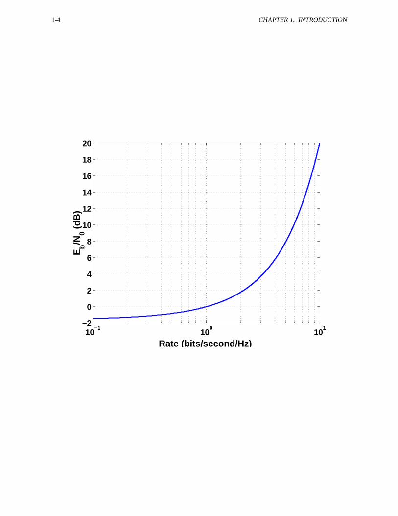
More than 50 years ago Claude Shannon (U of M EE/Math graduate) determined the tradeoff between datarate, bandwidth, signal power and noise power for reliable communications for an additive white Gaussian noisechannel. Let W be the bandwidth (in Hz), R be the data rate (in bits per second), P be the received signal power (inwatts) and N0 � 2 the noise power spectral density (in watts/Hz) then reliable communication is possible provided
R � W log2�1 � P
N0W
���
Let Eb be the energy transmitted per bit of information. Then
Eb � P � R or P � EbR�
Using this relation we can express the capacity formula as
R � W � log2�1 � Eb
N0
RW
���
Inverting this we obtain
Eb � N0 � 2R W 1R � W
�
The interpretation is that reliable communication is possible with bandwidth efficiency R � W provided that thesignal-to-noise ratio Eb � N0 is larger than the right hand side of the above equation. Usually energy or power ratiosare expressed in dB’s. The conversion is
Eb � N0�dB
� � 10log10�Eb � N0
���
The capacity formula only provides a tradeoff between energy efficiency and bandwidth efficiency. Complexityis essentially infinite, as is delay. The model of the channel is rather benign in that no signal fading is assumed tooccur.
1-4 CHAPTER 1. INTRODUCTION
10−1
100
101
−2
0
2
4
6
8
10
12
14
16
18
20
Rate (bits/second/Hz)
Eb/N
0 (d
B)
Chapter 2
Optimum Receiver Principles
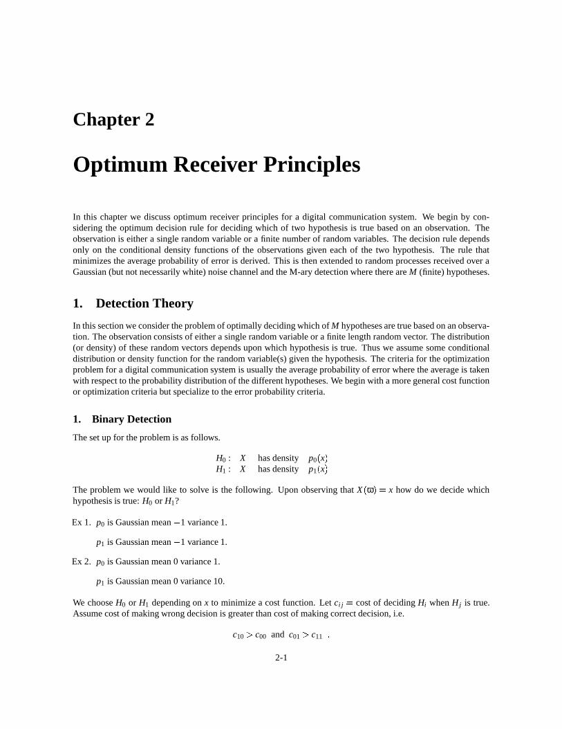
In this chapter we discuss optimum receiver principles for a digital communication system. We begin by con-sidering the optimum decision rule for deciding which of two hypothesis is true based on an observation. Theobservation is either a single random variable or a finite number of random variables. The decision rule dependsonly on the conditional density functions of the observations given each of the two hypothesis. The rule thatminimizes the average probability of error is derived. This is then extended to random processes received over aGaussian (but not necessarily white) noise channel and the M-ary detection where there are M (finite) hypotheses.
1. Detection Theory
In this section we consider the problem of optimally deciding which of M hypotheses are true based on an observa-tion. The observation consists of either a single random variable or a finite length random vector. The distribution(or density) of these random vectors depends upon which hypothesis is true. Thus we assume some conditionaldistribution or density function for the random variable(s) given the hypothesis. The criteria for the optimizationproblem for a digital communication system is usually the average probability of error where the average is takenwith respect to the probability distribution of the different hypotheses. We begin with a more general cost functionor optimization criteria but specialize to the error probability criteria.
1. Binary Detection
The set up for the problem is as follows.
H0 : X has density p0�x�
H1 : X has density p1�x�
The problem we would like to solve is the following. Upon observing that X�ω� � x how do we decide which
hypothesis is true: H0 or H1?
Ex 1. p0 is Gaussian mean 1 variance 1.
p1 is Gaussian mean � 1 variance 1.
Ex 2. p0 is Gaussian mean 0 variance 1.
p1 is Gaussian mean 0 variance 10.
We choose H0 or H1 depending on x to minimize a cost function. Let ci j � cost of deciding Hi when H j is true.Assume cost of making wrong decision is greater than cost of making correct decision, i.e.
c10 � c00 and c01 � c11�
2-1

2-2 CHAPTER 2. OPTIMUM RECEIVER PRINCIPLES
Let
π0 � probability that H0 is true�
π1 � probability that H1 is true�
Let C � cost of decision. Then
E � C � �1
∑i � 0
1
∑j � 0
ci jP�decide Hi � H j true � P
�H j �
� c00 P�decide H0 � H0 � P
�H0 �
� c01 P�decide H0 � H1 � P
�H1 �
� c10 P�decide H1 � H0 � P
�H0 �
� c11 P�decide H1 � H1 � P
�H1 � �
Let PF denote the probability of deciding H1 when actually H0 is true. This is usually called the probability of falsealarm. Let PD be the probability of deciding H1 is true when H1 is true. This is called the probability of detection.Let PM be the probability of deciding H0 is true when H1 is true. This is called the probability of miss.
PF � P�decide H1 � H0 � � 1 P
�decide H0 � H0 �
PD � P�decide H1 � H1 � � 1 P
�decide H0 � H1 � �
The average cost can be written in terms of the probability of false alarm and the probability of detection as follows.
E � C � � c00 � 1 PF � π0 � c01 � 1 PD � π1 � c10 � PF � π0 � c11PDπ1
� c00π0 � c01π1 � �c10
c00�π0 PF � �
c01 c11
�PDπ1
�
The term c00π0 � c01π0 represents a fixed cost that does not depend on what the decision made is nor does it dependon what the observation X is. Each of the last two terms are nonnegative.
Let R0 � the region of real line such that if X�ω� � x � R0 then the decision H0 is made. Similarly let R1 �
the region of real line such that if X�ω� � x � R1 then the decision H1 is made. We now write the false alarm and
detection probabilities in terms of these regions.
PF ��
R1
p0�x�dx � PD �
�R1
p1�x�dx
�
The average cost can now be written as
E � C � � c00π0 � c01π1 ��
R1
� � c10 c00
�π0 p0
�x� �
c01 c11
�π1 p1
�x� � dx
�
We wish to minimize the average cost. The expected cost as seen above is a constant c00π0 � c01π1 (independentof the decision region) plus an integral over the region R1 of a function depending on the densities of the observationgiven each hypothesis.
x
�c10
c00�π0 p0
�x� �
c01 c11
�π1 p1
�x� �

1. 2-3
We can minimize the average cost by choosing the decision region R1 to be that region for which the integrandis negative. Thus the optimal decision rule is to decide H1 if X � x and
�c10
c00�π0 p0
�x� �
c01 c11
�π1 p1
�x� � 0
�
Let
Λ�x� � p1
�x�
p0�x� �
The optimal decision rule can be rewritten as
Decide H1 if Λ�X� �
�c10
c00�π0�
c01 c11
�π1
Decide H0 if Λ�X� �
�c10
c00�π1�
c01 c11
�π0
�
Equivalently
�X� H1��
H0
�c01
c11�π0�
c10 c00
�π1
�
Λ�X�
is called the likelihood ratio. This is Bayes solution if π0 � π1 are known to the person designing the test.If we assign costs so that the performance measure is the average error probability (c0 � 1 � c1 � 0 � 1 � c0 � 0 �
c1 � 1 � 0) then the likelihood ratio test has the form
Λ�X� � p1
�X�
p0�X�
H1� �H0
π0
π1
p1�X�π1
H1� �H0
p0�X�π0
Decision rule is choose i so that pi�x�πi � p j
�x�π j
�j �� i. Equivalently the optimal decision rule can be described
as choose i so that p�i � x � � p
�j � x � �
j �� i where p�i � x � is the aposteriori probability of hypothesis i given the
observation x. The decision rule is thus to choose the hypothesis that maximizes the aposteriori probability. Thisis called the maximum aposteriori probability rule or MAP rule.Example 1:
p0�x� � ae � ax �
p1�x� � be � bx �
where a � b. The likelihood ratio for this test is
Λ�x� � p1
�x�
p0�x� � be � bx
ae � ax � ba
exp�x�a b
� �H1��H0
�c10
c00�π0�
c01 c11
�π1
∆� γ
ba
ex � a � b �H1� �H0
γ
ex � a � b �H1� �H0
aγb
x�a b
� H1� �H0
lnaγb
xH1� �H0
ln�aγ � b
��a b
� �

2-4 CHAPTER 2. OPTIMUM RECEIVER PRINCIPLES
The probability of false alarm and detection for the optimal decision rule can be determined as follows.
PF � P�Λ�X� � γ � H0 � � P
�X � ln
�aγ � b
��a b
� � H0 �
�� ∞
ln � aγ � b �� a � b � ae � axdx � e � ax
����� ∞ln � aγ � b �� a � b �� e � a ln � aγ � b �� a � b � �
PD � P�Λ�X� � γ � H1 � � P
�X � ln
�aγ � b
�a b � H1 �
� ∞
ln � aγ � b �a � b
be � bx � e � bx
����� ∞ln � aγ � b �� a � b �� exp
� b ln
�aγ � b
��a b
��� �
E � C � � � c00 � �c10
c00�PF � π0 � � c11
�c01
c11�PD � π1
�
For error probability criterion c00 � c11 � 0 c01 � c10 � 1�
Example 2:
H0 : X � �00000000
� � �0��
N
H1 : X � �11111111
� � �1��
N
where N � �N1 � � � � NL
�is a random noise vector with each component being 0 or 1 with P
�N1 � 0 � � 1
ρ � P�N1 � 1 � � ρ. Also N1 � � � � � NL is an i.i.d. sequence. The likelihood ratio for the observation X can be
determined as follows.
P�X � x � H0 � � ρ j � 1 ρ
� L � j wH�x� � j
P�X � x � H1 � � ρL � j � 1 ρ
� j wH�x� � j
Λ�j� � P
�X has j ones � H1 �
P�X has j ones � H0 � � L
L � j � ρL � j � 1 ρ� j
Lj � ρ j�1 ρ
�L � j�
ρ1 ρ L � 2 j H1� �
H01
�L 2 j
�log � ρ � �
1 ρ� �
H1� �H0
0�
Assume ρ � 1 � 2 � ρ � �1 ρ
� � 1 � log�ρ � �
1 ρ� � � 0. Thus the likelihood ratio test becomes
j
H1��H0
L2
�
If j � L � 2 then flip a coin. (This is obvious rule!)Example 3:
H0 : Xi � ni i � 0 � 1 � 2 � � � � � NH1 : Xi � si � ni i � 0 � 1 � 2 � � � � � L
� ni i � L � 1 � � � � � N

1. 2-5
where ni � 0 � i � N is sequence of i.i.d. Gaussian random variables mean 0 variance σ2.
p0�x� �
N
∏i � 0
p0�xi� �
N
∏i � 0
1�2πσ
e � � x2i 2σ2 �
� 1� �2πσ
�N
exp
� N
∑i � 0
x2i � 2σ2 �
p1�x� �
N
∏i � 0
p1�xi� �
L
∏i � 0
1�2πσ
e � � � xi � si � 2 2σ2 � N
∏i � L � 1
1�2πσ
e � x2i 2σ2
� 1� �2πσ
�N
exp
� 1
2σ2 � L
∑i � 0
�xi
si� 2 �
N
∑i � L � 1
x2i � �
p1�x�
p0�x� � exp
� 1
2σ2 � L
∑i � 0
�xi
si� 2 x2
i � �� exp
� 1
2σ2
L
∑i � 0
x2i 2xisi � s2
i x2
i�
� exp
� 1
2σ2
L
∑i � 0
s2i 2xisi
� H1��H0
γ
12σ2
L
∑i � 0
2xisi s2
i
H1��H0
lnγ
L
∑i � 0
xisi
H1��H0
12 � 2σ2 lnγ �
L
∑i � 0
s2i � �
2. Sufficient Statistic
In deciding which of two (or more) hypothesis is true based on a set of observations X1 � � � � � Xn in many cases thelikelihood ratio depends not on each individual Xi but on some function of the observations. For example, in thelast example of the previous subsection the likelihood ratio depended only on
S�x� �
L
∑i � 0
xisi
So if we do not know the individual values of x1 � � � � � xL but know S�x�
then that is sufficient information to makethe optimal decision about which hypothesis is true.Definition: Let X be a random variable (vector) whose distribution depends on a parameter θ � Θ (e.g. Θ � �
0 � 1 � ).A function S
�x�
is said to be sufficient for θ if the conditional distribution of X given S � s is independent of θ.
pθ�x � s � � p
�x � s � � θ � Θ pθ
�x� � gθ
�s�x� �
h�x�
θ � Θ�
(See Ferguson, pg. 115).Example:
Consider the repetition code example 2 above where
P�Xi � 1 � θ � 0 � � ρ
P�Xi � 0 � θ � 0 � � 1 ρ
P�Xi � 1 � θ � 1 � � 1 ρ
P�Xi � 0 � θ � 1 � � ρ

2-6 CHAPTER 2. OPTIMUM RECEIVER PRINCIPLES
and�Xi; i � 1 � � � � � L 1 � are conditionally independent (given θ). The sufficient statistic in this case is S � ∑L � 1
i � 0 Xi.To see this consider P
�X0 � x0 � � � � � XL � 1 � xL � 1 � S � l � θ � k � for k � 0 � 1
P�X0 � x0 � � � � � XL � 1 � xL � 1 � S � l � θ � k � � P
�X0 � x0 � � � � � XL � 1 � xL � 1 � S � l � θ � k �
P�S � l � θ � k �
P�X0 � x0 � � � � � XL � 1 � xL � 1 � S � l � θ � k � ���� � 0 � l �� ∑L � 1
i � 0 xi
pl � 1 p� L � l � k � 0 � l � ∑L � 1
i � 0 xi
pL � l � 1 p� l � k � 1 � l � ∑L � 1
i � 0 xi
P�S � l � θ � k � �
� Ll � pl � 1 p� L � l � k � 0 Ll � pL � l � 1 p
� l � k � 1�
Thus
P�X0 � x0 � � � � � XL � 1 � xL � 1 � S � l � θ � k � �
�0 � l �� ∑L � 1
i � 0 xi
Ll � � 1 � l � ∑L � 1i � 0 xi
Thus P�X0 � x0 � � � � � XL � 1 � xL � 1 � S � l � θ � k � does not depend on k so S is a sufficient statistic.
3. M-ary Detection Problem
Now consider the problem of deciding which of M hypothesis is true based on observing a random variable. Forthis case we restrict the performance criteria to be the average error probability. First we write the symbol errorprobability Pe � s in terms of the conditional density functions of the observations as follows.
Pe � s � E � C � �M � 1
∑i � 0
� ∑j �� i
P�decide H j � Hi true � � πi
�M � 1
∑i � 0
� 1 P�decide Hi � Hi true � � πi
�M � 1
∑i � 0
πi M � 1
∑i � 0
�Ri
pi�x�πidx
� 1 M � 1
∑i � 0
�Ri
pi�x�πidx
�
We conclude that the decision rule that minimizes average cost assigns x to Ri if pi�x�πi � max
0 � j � M � 1p j
�x�π j.
Thus for M hypotheses the decision rule that minimizes average error probability is to choose i so that pi�x�πi �
p j�x�π j � �
j �� i. Let
Λi � j � pi�x�
p j�x�
where i � 0 � 1 � � � � � M 1, j � 0 � 1 � � � � � M 1. Then the optimal decision rule is:
Choose i if Λi � j � π j
πifor all j �� i
�
We will usually assume πi � 1M
�i. (If not we should do source encoding to reduce the entropy (rate)). For this
case the optimal decision rule is
Choose i if Λi � j � 1�
j �� i�

2. 2-7
2. Likelihood Ratio for Random Processes
In this section we explore the extension of the detection process to waveforms (as opposed to finite dimensionalrandom vectors). Consider the simple binary detection problem
H0 : x�t� � x0
�t�
H1 : x�t� � x1
�t�
where x0�t� � x1
�t�
are random processes with presumably different statistics. For example, x0�t�
could be a (de-terministic) signal s0
�t�
plus additive white Gaussian noise while x1�t�
could be a signal s1�t�
plus additive whiteGaussian noise. The goal is to determine a decision rule based on observing x
�t�
to decide if H0 or H1 is true. Theidea is to represent the observation (a random process) using the Karhunen-Loeve transform as an infinite sequenceof independent random variables.
H0 : x�t� � ∑∞
l � 0 xlφl�t�
xl has density p0�xl�
H1 : x�t� � ∑∞
l � 0 xlφl�t�
xl has density p1�xl���
Here the random variables xl have different density functions depending on which hypothesis is true. Since theKarhunen-Loeve transform represents the random process by a infinite sequence of independent random variablesthe likelihoods for a finite set of these random variables is a product of the individual conditional density functionsfor these variables. So consider the likelihood of a finite number of these random variables:
p � N �0
�x� �
N
∏l � 0
p0�xl���
If we let N become large then the likelihood goes to zero. However if we first normalize the product by anotherdensity function, say p � N � � x � which also goes to zero and is the same for each hypothesis we can obtain somethingmeaningful when we take the limit of N � ∞. This is illustrated in the following example.
1. Example
Three signals in additive white Gaussian noise For additive white Gaussian noise K�s � t � � N0
2 δ�t s
�. Let�
ϕi�t� � ∞
i � 0 be any complete orthonormal set on � 0 � T � . Consider the case of 3 signals. Find the decision ruleto minimize average error probability. First expand the noise using orthonormal set of functions and randomvariables.
n�t� �
∞
∑i � 0
niϕi�t�
where E � ni � � 0 and Var � ni � � N0 � 2 and�ni � ∞
i � 0 is an independent identically distributed (i.i.d.) sequence ofrandom variables with Gaussian density functions.
Let
s0�t� � ϕ0
�t� � 2ϕ1
�t�
s1�t� � 2ϕ0
�t� � ϕ1
�t�
s2�t� � ϕ0
�t� 2ϕ1
�t�
Note that the energy of each of the three signals is the same, i.e.� T
0 s2i
�t�dt � � � si � � 2 � 5. Then we have a three
hypothesis testing problem.
H0 : r�t� � s0
�t� � n
�t� �
∞
∑i � 0
�s0 � i � ni
�ϕi
�t�
H1 : r�t� � s1
�t� � n
�t� �
∞
∑i � 0
�s1 � i � ni
�ϕi
�t�
H2 : r�t� � s2
�t� � n
�t� �
∞
∑i � 0
�s2 � i � ni
�ϕi
�t�
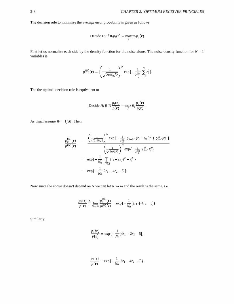
2-8 CHAPTER 2. OPTIMUM RECEIVER PRINCIPLES
The decision rule to minimize the average error probability is given as follows
Decide Hi if πi pi�r� � max
jπ j p j
�r�
First let us normalize each side by the density function for the noise alone. The noise density function for N � 1variables is
p � N � � r � � � 1�2πN0 � 2
� N
exp� 1
2 N02
N
∑i � 0
r2i �
The the optimal decision rule is equivalent to
Decide Hi if πipi
�r�
p�r� � max
jπ j
p j�r�
p�r� �
As usual assume πi � 1 � M. Then
p � N �0
�r�
p � N � � r � �
�1�
2πN0 2 N
exp� 1
2N02
� ∑i � 0 � 1�ri
s0 � i� 2 � ∑N
i � 3 r2i � ��
1�2πN0 2 N
exp� 1
2N02
∑Ni � 0 r2
i �
� exp� 1
N0� ∑i � 0 � 1
�ri
s0 � i� 2 r2
i � �
� exp� � 1
N0� 2r1 � 4r2
5 � � �
Now since the above doesn’t depend on N we can let N � ∞ and the result is the same, i.e.
p0�r�
p�r� ∆� lim
N � ∞
p � N �0
�r�
p � N � � r � � exp� � 1
N0� 2r1 � 4r2
5 � � �
Similarly
p1�r�
p�r� � exp
� � 1N0
� 4r1 � 2r2 5 � �
p2�r�
p�r� � exp
� � 1N0
� 2r1 4r2
5 � � �

2. 2-9
s0�t�
s1�t�
s2�t�
φ1�t�
φ2�t�
The decision regions are illustrated in the above figure. Note that the decision rule does not depend on thevalues of r3 � r4 � � � � . These variables are irrelevant when it comes to making an optimal decision. The optimaldecision rule is to compute r1 and r2 and then find the maximum of r1 � 2r2, 2r1 � r2, r1
2r2 and then decideH0 H1 or H2 depending on which one is largest. The overall receiver is then shown in the below figure. Thereare clearly many implicit assumptions in this receiver diagram. One of these assumptions is that we are able tosyncronize the correlating waveforms φl
�t�
to the incoming signal. Another of these is perfect integration over thetime span of the waveform. An alternate implementation whereby the multiplier and integrator are replaced with amatched filter is also possible.
r�t�
�
�
φ1�t�
φ2�t�
� ��� �dt
� ��� �dt
� ��� �dt
Chooselargestr1 � 2r2
2r1 � r2
r1 2r2
r1
r2
Figure 2.1: Optimum Receiver

2-10 CHAPTER 2. OPTIMUM RECEIVER PRINCIPLES
3. Detection with Unwanted Parameters
In this section we consider the problem of detection with unwanted parameters. To illustrate consider the problemof minimizing the bit error probability in an M-ary orthogonal signal set.
Let s0�t� � � � � � sM � 1
�t�
be orthogonal signals.
s0�t� �
�Eφ0
�t�
s1�t� �
�Eφ1
�t�
� �� �� �
sM � 1�t� �
�EφM � 1
�t�
Let b0 � � � � � bk � 1 be the sequence of bits determining which of the M signals is transmitted. Assume the bits areindependent and equally likely.
The receiver consists of a bank of matched filters (correlators) that generate a sufficient statistic. If signal s j istransmitted then
r0 � δ�j � 0 � �
E � η0
r1 � δ�j � 1 � �
E � η1� �� �� �� �
rM � 1 � δ�j � M 1
� �E � ηM � 1
Consider the detection of data bit b0. That is, we are interested in minimizing the probability of error for data bitb0. Let H0 be the event that b0 � 0 and H1 be the event that b0 � 1. Let r � �
r0 � r1 � � � � rM � 1�. Then the optimal
receiver must compare the two aposteriori probabilities
p�r � H0
�π0
H0��H1
p�r � H1
�π1
To calculate p�r � H0
�we proceed as follows.
p�r � H0
�π0 � p
�r � b0 � 0
�π0
� π0 ∑b1 � � � � � bk � 1
p�r � b0 � 0 � b1 � � � � bk � 1
�p�b1
�p�b2
� �����p�bk
�
� 2 � k ∑b1 � � � � � bk � 1
� 1�2πσ
� M exp� 1
2σ2
M � 1
∑l � 0
�rl
s�b� � 2 �
� 2 � kM 2
∑m � 0
� 1�2πσ
� M exp� 1
2σ2
M � 1
∑l � 0
�rl
δ�l � m � �
E� 2 �
� 2 � k � 1�2πσ
� MM 2
∑m � 0
exp� 1
2σ2
M � 1
∑l � 0
�rl
δ�l � m � �
E� 2 �
� 2 � k � 1�2πσ
� MM 2
∑m � 0
exp� 1
2σ2
M � 1
∑l � 0
�r2
l 2rlδ
�l � m � �
E � δ�l � m �
E �

4. 2-11
� 2 � k � 1�2πσ
� M exp� 1
2σ2
M � 1
∑l � 0
r2l � exp
� E � 2σ2 �M 2
∑m � 0
exp� 1
σ2
M � 1
∑l � 0
�rlδ
�l � m � �
E �
� 2 � k � 1�2πσ
� M exp� 1
2σ2
M � 1
∑l � 0
r2l � exp
� E � 2σ2 �M 2
∑m � 0
exp� rm
�E
σ2 �
Similarly
p�r � H1
�π1 � p
�r � b0 � 1
�π1
� 2 � k � 1�2πσ
� M exp� 1
2σ2
M � 1
∑l � 0
r2l � exp
� E � 2σ2 �M � 1
∑m � M 2 � 1
exp� rm
�E
σ2 �
Notice that many of the factors in p�r � H1
�π1 and p
�r � H1
�π1 are the same. Thus the likelihood ratio for bit b0 is
p�r � H1
�π1
p�r � H0
�π0
�∑M � 1
m � M 2 � 1 exp� rm
�E
σ2 �∑M 2
m � 0 exp� rm
�E
σ2 �The log-likelihood ratio is
log� p
�r � H1
�π1
p�r � H0
�π0
� � log� M � 1
∑m � M 2 � 1
exp� rm
�E
σ2 � � log� M 2
∑m � 0
exp� rm
�E
σ2 � �
This can be approximated by
log� p
�r � H1
�π1
p�r � H0
�π0
��� M � 1max
m � M 2 � 1
�rm
�E � σ2 � M 2
maxm � 0
�rm
�E � σ2 �
4. Likelihood Ratio for Real Signals
In this section we consider the general binary problem of detecting one of two real signals in additive Gaussiannoise.
H0 : r�t� � s0
�t� � n
�t�
H1 : r�t� � s1
�t� � n
�t�
Let n�t�
have covariance K�s � t � with eigenfunction ϕi
�t�
and eigenvalues λi�n�t�
is also zero mean Gaussian).
By K L expansion n�t� �
∞
∑i � 1
niϕi�t�
where ni is a Gaussian random variable with mean 0 variance λi and
E � nin j � � 0 � ni � n j independent�n�t�
is real). Since ϕi�t�
are a complete orthonormal set and we assume s j�t�
has finite energy we have s j�t� �
∞
∑i � 0
s j � iϕi�t�. Thus
H j : r�t� �
∞
∑i � 0
�s j � i � ni
�ϕi
�t�
ri � s j � i � ni � i � 1 � 2 � � � �
Define
Λ j � i�N� ∆� p j
�r1 � r2 � � � � � rN
�pi�r1 � r2 � � � � � rN
� �
Λ j � i�r�t� � ∆� lim
N � ∞Λ ji
�N�
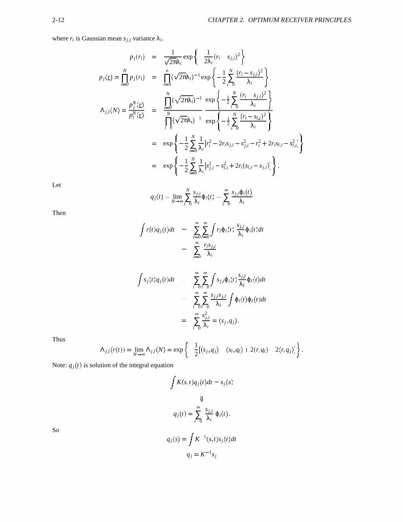
2-12 CHAPTER 2. OPTIMUM RECEIVER PRINCIPLES
where ri is Gaussian mean s j � i variance λi.
p j�ri� � 1�
2πλiexp
� 1
2λi
�ri
s j � i� 2 �
p j�r� �
N
∏i � 0
p j�ri� �
n
∏i � 0
� �2πλi
� � 1 exp
� 1
2
N
∑i � 0
�ri
s j � i� 2
λi
�Λ j � l
�N� �
pNj
�r�
pNl
�r� �
N
∏i � 0
� �2πλi
� � 1
N
∏i � 0
� �2πλi
� � 1
exp
� 1
2
N
∑i � 0
�ri
s j � i� 2
λi
�exp
� 1
2
N
∑i � 0
�ri
sl � i� 2
λi
�� exp
� 1
2
N
∑i � 0
1λi
� r2i 2ris j � i � s2
j � i r2i � 2risl � i s2
l � i � �� exp
� 1
2
N
∑i � 0
1λi
� s2j � i s2
l � i � 2ri�sl � i s j � i
� � � �
Let
q j�t� � lim
N � ∞
N
∑i � 0
s j � iλi
ϕi�t� �
∞
∑i � 0
s j � iϕi�t�
λi
Then�
r�t�q j
�t�dt �
∞
∑i � 0
∞
∑l � 0
�rlϕl
�t� s j � i
λiϕi
�t�dt
�∞
∑i � 0
ris j � iλi
�s j
�t�q j
�t�dt �
∞
∑i � 0
∞
∑l � 0
�s j � iϕi
�t� s j � l
λlϕl
�t�dt
�∞
∑i � 0
∞
∑l � 0
s j � is j � lλl
�ϕi
�t�ϕl
�t�dt
�∞
∑i � 0
s2j � i
λi� �
s j � q j���
Thus
Λ j � l�r�t� � � lim
N � ∞Λ j � l
�N� � exp
� 1
2� � s j � q j
� �sl � ql
� � 2�r� ql
� 2�r� q j
� � � �
Note: q j�t�
is solution of the integral equation�
K�s � t � q j
�t�dt � s j
�s�
�
q j�t� �
∞
∑i � 0
s j � iλi
ϕi�t���
Soq j
�s� �
�K � 1 � s � t � s j
�t�dt
q j � K � 1s j
4. 2-13
If the noise is white, then the noise power in each direction is constant (say λ) and thus
q j�t� �
∞
∑i � 0
s j � iλ
ϕi�t� � 1
λs j
�t���
The optimal receiver then becomes
Λ j � l�r�t� � � exp
� 1
2λ� � s j � s j
� �sl � sl
� � 2�r� sl
� 2�r� s j
� � � �
or equivalently
Λ j � l�r�t� � � exp
� 1
2λ� � � s j � � 2 � � sl � � 2 � 2
�r� sl
s j� � � �
For equal energy signals this amounts to picking the signal with the largest correlation with the received signal.
The optimal receiver in nonwhite Gaussian noise can be implemented in a similar fashion as shown below.
�s j � q j
� � �s j � K � 1s j
� � �K � 1 2s j � K � 1 2s j
� ��� K1 2s j � 2�r� q j
� � �r� K � 1s j
� � �K � 1 2r� K � 1 2s j
�
Thus
Λ j � l�r�t� � � exp
� 1
2� � � K � 1 2s j � � 2 � � K � 1 2sl � � 2 � 2
�K � 1 2r� K � 1 2 � sl
s j� � � � �
It is clear then that this is just the optimal filter for signals K � 1 2s j when received in additive white Gaussian noise.This approach is called “whitening” because K � 1 2n will be a white Gaussian noise process.

2-14 CHAPTER 2. OPTIMUM RECEIVER PRINCIPLES
5. Likelihood Ratio for Complex Signals
In this section we rederive the likelihood ratios for complex signals received in complex noise. We assume thatthe signals are the lowpass representation of bandpass signal and the noise is the lowpass representation of anarrowband random process. Let
H0 : r�t� � s0
�t� � n
�t�
H1 : r�t� � s1
�t� � n
�t�
where n�t�
has covariance K�s � t � , with eigenfunctions ϕi
�t�, eigenvalues λi. Using K L expansion we have
Hi : r�t� �
∞
∑j � 0
�si � j � n j
�ϕ j
�t�
r j � si � j � n j�
p j�r1 � � � � � rn
�pi�r1 � � � � � rn
� �∏n
l � 01
πλle � ��� rl � s j � l � 2 � λl
∏nl � 0
1πλl
e � ��� rl � si � l � 2 � λl
�n
∏l � 0
exp� � � rl
s j � l � 2 � rl sil � 2 � � λl �
� exp
� n
∑l � 0
� � rl s j � l � 2 � rl
si � l � 2 � � λl�
� exp
� n
∑l � 0
� rl � 2 � � s j � l � 2 2 Re�rls � j � l
� � rl � 2 � si � l � 2 � 2 Re�rls �i � l
�λl
�� exp
� n
∑l � 0
� s j � l � 2 � si � l � 2 � 2Re � rl�si � l s j � l
�� �
λl
� �
Let q j�t� �
∞
∑i � 0
s ji
λiϕi
�t�
then
�q j
�t� � s j
�t� � �
� b
a
∞
∑l � 0
s j � lλl
ϕl�t� ∞
∑k � 0
s � j � kϕ �k�t�dt
�∞
∑l � 0
� s j � l � 2 � λl � �s j
�t� � q j
�t� �
�r�t� � q j
�t� � �
� b
a
∞
∑l � 0
rlϕl�t� ∞
∑k � 0
s � j � kλk
ϕ �k�t�dt
�∞
∑l � 0
rls � j � lλl
�
So
Λ ji�r�t� � � lim
H � ∞Λ � n �
ji
�r�t� � � p j
�r1 � � � � � rn
�pi�r1 � � � � � rn
�� exp
� � � s j � q j� �
si � qi� � 2 Re
�r�t� � qi
�t� q j
�t� � �
Note: Since we are dealing with noise that is derived from a narrowband random process we can not use the resultsderived for real random processes we must use the likelihood ratio for complex random process given above.

6. 2-15
For real random process the likelihood ratio is
Λ ji�N� � exp
� 12
� � s j � q j� �
si � qi� � 2
�r� qi
q j� � � �
For additive white Gaussian noise (real)
qi�t� �
∞
∑j � 1
si � jϕ j�t�
λ j� 2
N0
∞
∑j � 1
si � jϕ j�t�
� 2N0
si�t�
So the likelihood ratio (for real signals) becomes
Λ j � l � limN � ∞
p j�r1 � � � � � rN
�pl
�r1 � � � � � rN
� � exp
� 1
2 � 2N0
� �s j � s j
� �sl � sl
� � � 2� 2N0
�r� sl
s j� � �
� exp
� 1
N0� � s j � 2 2
�r� s j
� � r � 2 � � sl � 2 2�r� sl
� � r � 2 � � �� exp
� 1
N0� � s j
r � 2 � sl r � 2 � � H j��
Hl
1�
Assume π j � 1M j � 1 � 2 � � � � � M. Then α � 1. An equivalent decision rule then is
� s j r � 2 � sl
r � 2Hl��H j
0
� s j r � 2
Hl��H j� sl
r � 2 �
The optimum decision rule for additive white Gaussian noise is then to choose i if
� si r � 2 � min
1 � j � M � s j r � 2 �
6. Example: M orthogonal signals in additive white Gaussian noise
In this section we consider the optimum receiver for M-ary orthogonal signals and the associated error probaib-lity. Assume the M signals are equienergy signals and equiprobable. The decision rule derived previously forAWGN is
Decide Hi if � � si r � � 2 � min
1 � j � M � � s j r � � 2 �
Now since the M signals are orthogonal and equienergy we can write this as
� � s j r � � 2 � � � s j � � 2 2
�s j � r � � � � r � � 2 �
The first term above is constant for each j as is the last term. Thus finding the minimum is equivalent to findingthe maximum of �
s j � r ���
Thus the receiver should compute the inner product between the M different signals and find the largest suchcorrelation. If the signals are all of duration T , i.e. zero outside the interval � 0 � T � then this is also equivalent tofiltering the received signal with a filter with impluse response s j
�T t
�, sampling the output of the filter at time
T and choosing the largest as shown below.

2-16 CHAPTER 2. OPTIMUM RECEIVER PRINCIPLES
7. Problems
1. (a) Consider any two binary signals s0�t� � s1
�t�
with Ei � � si�t� � 2 the energy of signal si
�t�
and
ρ � �s0 � s1
� � E
��
s0�t�s1
�t�dt � E
where E � �E0 � E1
� � 2 . Assume that signal s0�t�
is transmitted with probability π0 and signal s1�t�
istransmitted with probability π1 with π0 � π1 � 1. The received signal is the transmitted signal plus additivewhite Gaussian noise with two-sided power spectral density N0 � 2.
(a) Find the optimum receiver. (Do not assume that π0 � π1).
(b) Find the average error probability of the optimum receiver.
(c) If now π0 � π1 find the value of ρ that minimizes the error probability. (Note that by Schwarz’ inequality 1 � ρ � 1).
2. Consider the following hypothesis testing problem
H0 : X p0�x� � 1�
2πexp � �
x 1� 2 � 2 �
H1 : X p1�x� � 1�
2πexp � �
x � 1� 2 � 2 �
(a) Find the test that minimizes the average cost.
(b) If c00 � c11 � 0 and c01 � c10 � 1 and π0 � π1 what is the (minimum average cost) test?
3. Consider a hypothesis testing problem with three alternatives H0 � H1 � and H2. With ci j representing the costof deciding Hi is true when H j is true, find a test(s) that minimizes the average cost. (Let πi i � 0 � 1 � 2 be theprobability that Hi is true).
4. Find the test (decision rule) that minimizes average error probability for the following detection theoryproblem. Assume σ1 � σ0 and π0 � π1 � 1 � 2.
H0 : X p0�x� � 1�
2πσ0exp � x2 � �
2σ20� �
H1 : X p1�x� � 1�
2πσ1exp � x2 � �
2σ21� �
5. For the seven-signal set shown, transmitted over the additive white Gaussian noise (AWGN) channel, withequal a priori probabilities (πi � 1 � 7) and equal energies (for the six nonzero signals).
(a) Determine the optimum decision regions.
(b) Show that Pm � probability of error given signal m transmitted is upper bounded by the probability thatthe norm of the two dimensional noise vector is greater than
�E � 2.
(c) Using (b) find an upper bound on the average probability of error.
7. 2-17
�
�
�� �E
�E
�� �
� �
� �
6. A certain digital communication system transmits one of two signals s0, and s1 in additive (not necessarilywhite) Gaussian noise with covariance function K
�s � t � . Let φi be the eigenfunctions of K
�s � t � and let λi be
the corresponding eigenvalues.
(a) If s0�t� � A0φ0
�t�
and s1�t� � A1φ1
�t�
find the optimal receiver for minimizing the average error proba-bility.
(b) If the two signals are equally probable find the average error probability.
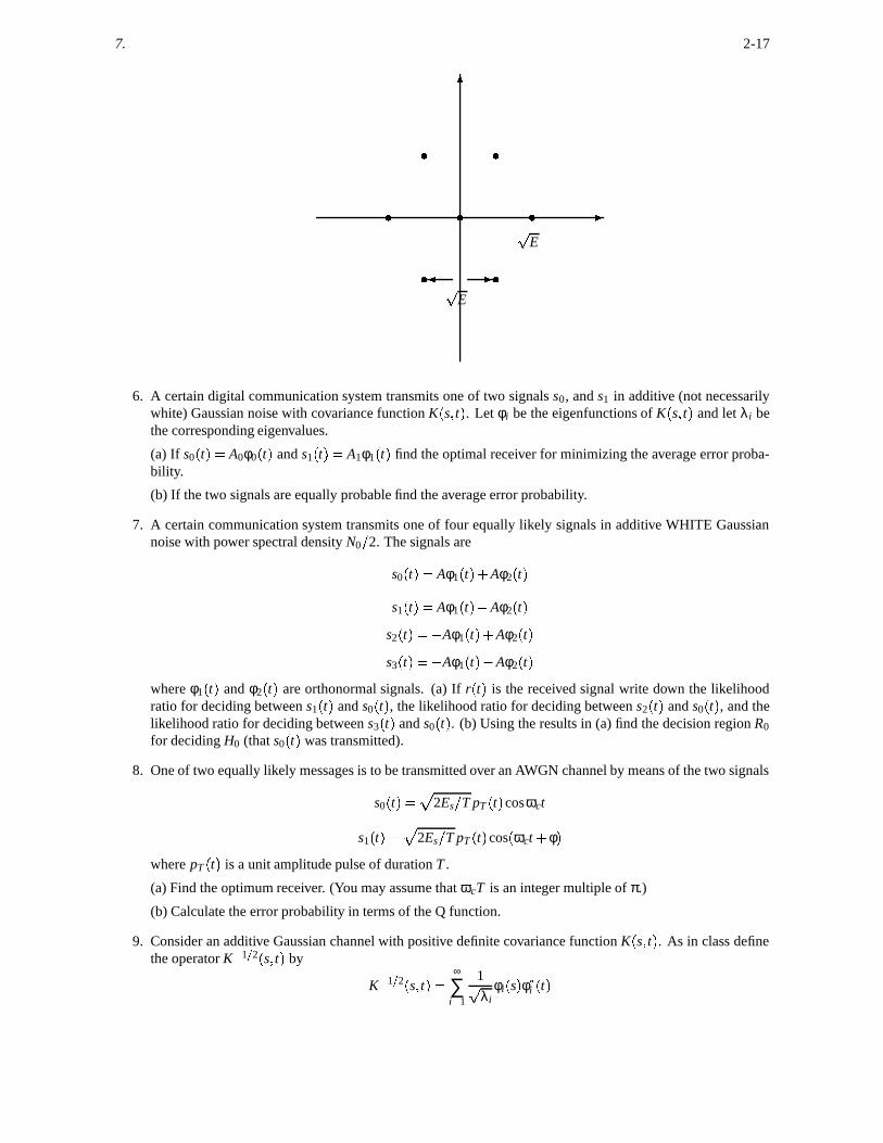
7. A certain communication system transmits one of four equally likely signals in additive WHITE Gaussiannoise with power spectral density N0 � 2. The signals are
s0�t� � Aφ1
�t� � Aφ2
�t�
s1�t� � Aφ1
�t� Aφ2
�t�
s2�t� � Aφ1
�t� � Aφ2
�t�
s3�t� � Aφ1
�t� Aφ2
�t�
where φ1�t�
and φ2�t�
are orthonormal signals. (a) If r�t�
is the received signal write down the likelihoodratio for deciding between s1
�t�
and s0�t�, the likelihood ratio for deciding between s2
�t�
and s0�t�, and the
likelihood ratio for deciding between s3�t�
and s0�t�. (b) Using the results in (a) find the decision region R0
for deciding H0 (that s0�t�
was transmitted).
8. One of two equally likely messages is to be transmitted over an AWGN channel by means of the two signals
s0�t� �
�2Es � T pT
�t�cosωct
s1�t� �
�2Es � T pT
�t�cos
�ωct � φ
�
where pT�t�
is a unit amplitude pulse of duration T .
(a) Find the optimum receiver. (You may assume that ωcT is an integer multiple of π.)
(b) Calculate the error probability in terms of the Q function.
9. Consider an additive Gaussian channel with positive definite covariance function K�s � t � . As in class define
the operator K � 1 2 � s � t � by
K � 1 2 � s � t � �∞
∑i � 1
1�λi
φi�s�φ �i
�t�

2-18 CHAPTER 2. OPTIMUM RECEIVER PRINCIPLES
(a) Show that for any two functions x�t� � y
�t�
(in L2 � a � b � ) that
�x � K � 1y
� � �K � 1 2x � K � 1 2y
�
(b) Consider a signal set�s j : j � 0 � 1 � � � � � M 1 � . Let s j � K � 1 2s j , j � 0 � 1 � � � � � M 1 and let r � K � 1 2r.
Consider the receiver which decides hypothesis Hi if
� � si r � � � min
0 � j � M � 1� � s j
r � �Using (a) (or otherwise) show that the above receiver is optimal for equiprobable signals.
10. Consider the binary symmetric channel with crossover probability p � 1 � 2. The input and output alphabetfor this channel is
�0 � 1 � . Consider a signal set
�si : 0 � i � M 1 � in n dimensions for this channel with
each coefficient (component) being 0 or 1, i.e. consider the signal as a vector of length n. Assume that allsignals are equally likely. Let r � �
r1 � � � � � rn�
be the received vector with ri � �0 � 1 � . For any two binary
vectors x and y let dH�x � y � = number of places where x and y differ.
(a) Show that the optimal receiver for minimizing average error probability is to chose that signal for whichdiffers from r in the fewest places i.e. decide hypothesis Hi if
dH�r � si
� � min0 � j � M � 1
dH�r � s j
�
(b) For any such signal set determine the union-Bhattacharrya bound for the optimal receiver. Your answershould depend on the distance between signals.
11. Consider a digital communication system that transmits one of two equally likely signals over a discrete timeadditive channel with nonwhite Gaussian noise. The two signals transmitted are
s0 � �1 � 1 � 1
�
ands1 � �
1 � 1 � 1 ���The noise added to each component of the signal is Gaussian but not independent nor identically distributed.The noise vector n � �
n0 � n1 � n2�
has zero mean and covariance matrix.
K ���
3 2 0 2 3 00 0 5
��
The covariance matrix has eigenvalues, λ1 � 5, λ2 � 5 and λ3 � 1 with corresponding (orthonormal) eigen-vectors
φ1 � � 1 ��
2 � 1 ��
2 � 0 � �φ2 � �
0 � 0 � 1 � �φ3 � �
1 ��
2 � 1 ��
2 � 0 ���
(a) Find the optimal receiver for minimizing the error probability between the two signals.
(b) Find the error probability for the optimal receiver.
12. Consider the following detection problem. Under hypothesis H0, X is zero mean Gaussian with variance σ2.Under hypothesis H1 is a mixture of two Gaussians with means +1 and -1, each with variance σ2 and themixture is uniform. That is under H1, X � α � η where α is a random variable equally likely to be � 1 andη is a zero mean Gaussian random variable. Find the optimal decision region for deciding which of the twoequally likely hypothesis is true in order to minimize the error probability.