eece 460 : control system design - siso pole placement · polynomial pole placement the diophantine...
TRANSCRIPT

EECE 460 : Control System DesignSISO Pole Placement
Guy A. Dumont
UBC EECE
January 2011
Guy A. Dumont (UBC EECE) EECE 460: Pole Placement January 2011 1 / 29

Contents
1 Preview
2 Polynomial Pole Placement
3 Constraining the Solution
4 PID Design
5 Smith Predictor
Guy A. Dumont (UBC EECE) EECE 460: Pole Placement January 2011 2 / 29

Preview
Preview
Formal control design method
The key synthesis question is:
Given a model, can one systematically synthesize a controller such that theclosed-loop poles are in predefined locations?
This is indeed possible through pole assignment
In EECE360, we saw a method for assigning closed-loop poles throughstate feedback (see review notes)
Here we shall see a polynomial approach based on transfer functions
This material is covered in Chapter 7 of the textbook
Guy A. Dumont (UBC EECE) EECE 460: Pole Placement January 2011 3 / 29
Polynomial Pole Placement
Polynomial Pole Placement
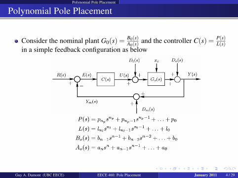
Consider the nominal plant G0(s) = B0(s)A0(s)
and the controller C(s) = P(s)L(s)
in a simple feedback configuration as below
Guy A. Dumont (UBC EECE) EECE 460: Pole Placement January 2011 4 / 29
Polynomial Pole Placement
The Design Objective
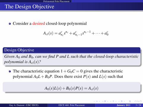
Consider a desired closed-loop polynomial
Acl(s) = acnc
snc +acnc−1snc−1 + · · ·+ac
0
Design ObjectiveGiven A0 and B0, can we find P and L such that the closed-loop characteristicpolynomial is Acl(s)?
The characteristic equation 1+G0C = 0 gives the characteristicpolynomial A0L+B0P. Does there exist P(s) and L(s) such that
A0(s)L(s)+B0(s)P(s) = Acl(s)
Guy A. Dumont (UBC EECE) EECE 460: Pole Placement January 2011 5 / 29
Polynomial Pole Placement
A Simple Example
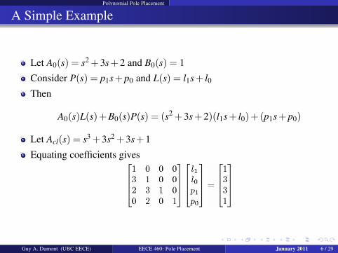
Let A0(s) = s2 +3s+2 and B0(s) = 1
Consider P(s) = p1s+p0 and L(s) = l1s+ l0Then
A0(s)L(s)+B0(s)P(s) = (s2 +3s+2)(l1s+ l0)+(p1s+p0)
Let Acl(s) = s3 +3s2 +3s+1
Equating coefficients gives
Guy A. Dumont (UBC EECE) EECE 460: Pole Placement January 2011 6 / 29

Polynomial Pole Placement
A Simple Example
The above 4×4 matrix is non-singular, hence it can be inverted and wecan solve for p0, p1, l0 and l1Doing so, we find l0 = 0, l1 = 1, p0 = 1 and p1 = 1
Hence the desired characteristic polynomial is achieved by the controller
C(s) =P(s)L(s)
=s+1
s
Note that this is a PI controller!
Note that in order to solve for the controller, a particular matrix has to benon-singular
This matrix is known as the Sylvester matrix
Guy A. Dumont (UBC EECE) EECE 460: Pole Placement January 2011 7 / 29
Polynomial Pole Placement
Sylvester’s Theorem
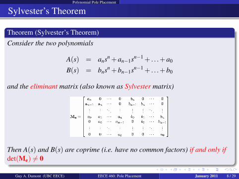
Theorem (Sylvester’s Theorem)Consider the two polynomials
A(s) = ansn +an−1sn−1 + . . .+a0
B(s) = bnsn +bn−1sn−1 + . . .+b0
and the eliminant matrix (also known as Sylvester matrix)
Then A(s) and B(s) are coprime (i.e. have no common factors) if and only ifdet(Me) 6= 0
Guy A. Dumont (UBC EECE) EECE 460: Pole Placement January 2011 8 / 29
Polynomial Pole Placement
Pole Placement Design
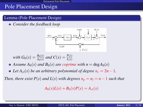
Lemma (Pole Placement Design)Consider the feedback loop
with G0(s) = B0(s)A0(s)
and C(s) = P(s)L(s)
Assume A0(s) and B0(s) are coprime with n = degA0(s)Let Acl(s) be an arbitrary polynomial of degree nc = 2n−1.
Then, there exist P(s) and L(s) with degrees np = nl = n−1 such that
A0(s)L(s)+B0(s)P(s) = Acl(s)
Guy A. Dumont (UBC EECE) EECE 460: Pole Placement January 2011 9 / 29

Polynomial Pole Placement
The Diophantine Equation
The equationA0(s)L(s)+B0(s)L(s) = Acl(s)
is called Diophantine equation after Greek mathematician Diophantus1.
In its matrix form, it is also referred to as the Bezout Identity. It plays acentral role in modern control theory.
The previous Lemma presents the solution for the minimal complexitycontroller.
The controller is said to be biproper, i.e. degP(s) = degL(s)Usually, the polynomials A0(s), L(s) and Acl(s) are monic i.e. coefficientof highest power of s is unity.
1Diophantus, often known as the ’father of algebra’, is best known for his Arithmetica, awork on the solution of algebraic equations and on the theory of numbers. However, essentiallynothing is known of his life and there has been much debate regarding the date at which helived.
Guy A. Dumont (UBC EECE) EECE 460: Pole Placement January 2011 10 / 29

Constraining the Solution
Forcing Integration
As seen before, it is very common to force the controller to contain anintegrator
To achieve this, we need to rewrite the denominator of the controller as
L(s) = sL(s)
The Diophantine equation
A0(s)L(s)+B0(s)P(s) = Acl(s)A0(s)sL(s)+B0(s)P(s) = Acl(s)
can then be rewritten as
Forcing Integration
A0(s)L(s)+B0(s)P(s) = Acl(s) with A0(s) = sA0(s)
Guy A. Dumont (UBC EECE) EECE 460: Pole Placement January 2011 11 / 29

Constraining the Solution
Forcing Integration
Note that because we have increased the degree of the l.h.s. by 1, nowwe have degAcl = 2n and need to add a closed-loop pole.
Also, since degL = deg L+1, to keep a bi-proper controller, we shouldhave degP = degL = deg L+1
Guy A. Dumont (UBC EECE) EECE 460: Pole Placement January 2011 12 / 29
Constraining the Solution
Forcing Pole/Zero Cancellation
Sometimes it is desirable to force the controller to cancel a subset ofstable poles or zeros of the plant model
Say we want to cancel a process pole at −p, i.e. the factor (s+p) in A0,then P(s) must contain (s+p) as a factor.
Then the Diophantine equation has a solution if and only if (s+p) is alsoa factor of Acl
To solve the resulting Diophantine equation, the factor (s+p) is simplyremoved from both sides
Guy A. Dumont (UBC EECE) EECE 460: Pole Placement January 2011 13 / 29
Constraining the Solution
Example 1
Consider the system
G0(s) =3
(s+1)(s+3)
The unconstrained problem calls for degAcl = 2n−1 = 3. ChooseAcl(s) = (s2 +5s+16)(s+40). The polynomials P and L are of degree1. The Diophantine equation is
(s+1)(s+3)(s+ l0)+3(p1s+p0) = (s2 +5s+16)(s+40)
which yields l0 = 41, p1 = 49/3 and p0 = 517/3 and the controller C(s)is
C(s) =49s+5173(s+41)
Guy A. Dumont (UBC EECE) EECE 460: Pole Placement January 2011 14 / 29
Constraining the Solution
Example 1
Consider now the constrained case where we want the controller tocontain integration. We need to add a closed-loop pole. Let us say thatwe want the controller to cancel the process pole at −1. The Diophantineequation then becomes
(s+1)(s+3)s(s+ l0)+3(s+1)(p1s+p0) = (s+1)(s2 +5s+16)(s+40)
which after eliminating the common factor (s+1) yields l0 = 42,p1 = 30 and p0 = 640/3 and the controller C(s) is
C(s) =(s+1)(90s+640)
3s(s+42)
Guy A. Dumont (UBC EECE) EECE 460: Pole Placement January 2011 15 / 29
Constraining the Solution
Example 2
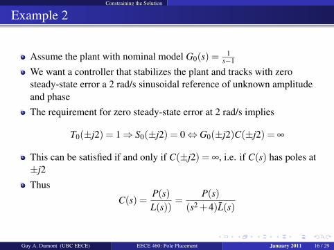
Assume the plant with nominal model G0(s) = 1s−1
We want a controller that stabilizes the plant and tracks with zerosteady-state error a 2 rad/s sinusoidal reference of unknown amplitudeand phase
The requirement for zero steady-state error at 2 rad/s implies
T0(±j2) = 1⇒ S0(±j2) = 0⇔ G0(±j2)C(±j2) = ∞
This can be satisfied if and only if C(±j2) = ∞, i.e. if C(s) has poles at±j2
Thus
C(s) =P(s)L(s))
=P(s)
(s2 +4)L(s)
Guy A. Dumont (UBC EECE) EECE 460: Pole Placement January 2011 16 / 29
Constraining the Solution
Example 2
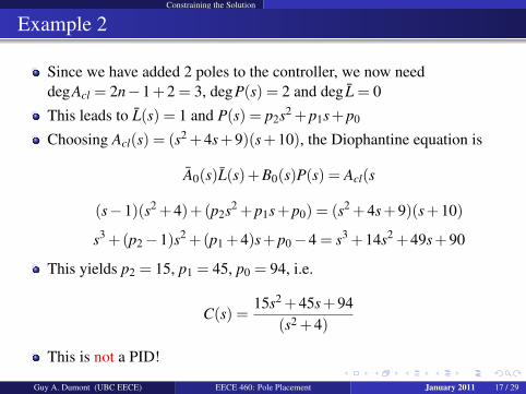
Since we have added 2 poles to the controller, we now needdegAcl = 2n−1+2 = 3, degP(s) = 2 and deg L = 0
This leads to L(s) = 1 and P(s) = p2s2 +p1s+p0
Choosing Acl(s) = (s2 +4s+9)(s+10), the Diophantine equation is
A0(s)L(s)+B0(s)P(s) = Acl(s
(s−1)(s2 +4)+(p2s2 +p1s+p0) = (s2 +4s+9)(s+10)
s3 +(p2−1)s2 +(p1 +4)s+p0−4 = s3 +14s2 +49s+90
This yields p2 = 15, p1 = 45, p0 = 94, i.e.
C(s) =15s2 +45s+94
(s2 +4)
This is not a PID!
Guy A. Dumont (UBC EECE) EECE 460: Pole Placement January 2011 17 / 29
PID Design
Pole-Placement PID Design
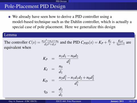
We already have seen how to derive a PID controller using amodel-based technique such as the Dahlin controller, which is actually aspecial case of pole placement. Here we generalize this design
Lemma
The controller C(s) = n2s2+n1s+n0d2s2+d1s and the PID CPID(s) = KP + KI
s + KDsτDs+1 are
equivalent when
KP =n1d1−n0d2
d21
KI =n0
d1
KD =n2d2
1−n1d1d2 +n0d22
d31
τD =d2
d1
Guy A. Dumont (UBC EECE) EECE 460: Pole Placement January 2011 18 / 29

PID Design
Pole-Placement PID Design
To obtain a PID controller, we then need to use a delay-free second-ordernominal model for the plant and design a controller forcing integration
We thus choose
degA0(s) = 2
degB0(s) ≤ 1
deg L(s) = 1
degP(s) = 2
degAcl = 4
Guy A. Dumont (UBC EECE) EECE 460: Pole Placement January 2011 19 / 29
PID Design
Example 3
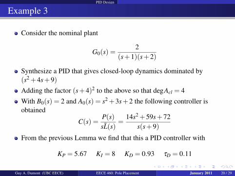
Consider the nominal plant
G0(s) =2
(s+1)(s+2)
Synthesize a PID that gives closed-loop dynamics dominated by(s2 +4s+9)Adding the factor (s+4)2 to the above so that degAcl = 4
With B0(s) = 2 and A0(s) = s2 +3s+2 the following controller isobtained
C(s) =P(s)sL(s)
=14s2 +59s+72
s(s+9)
From the previous Lemma we find that this a PID controller with
KP = 5.67 KI = 8 KD = 0.93 τD = 0.11
Guy A. Dumont (UBC EECE) EECE 460: Pole Placement January 2011 20 / 29

PID Design
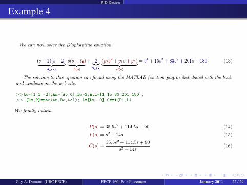
Example 4
Guy A. Dumont (UBC EECE) EECE 460: Pole Placement January 2011 21 / 29
PID Design
Example 4
Guy A. Dumont (UBC EECE) EECE 460: Pole Placement January 2011 22 / 29
Smith Predictor
The Smith Predictor
Of course, in general pole placement design will not yield a PID
This is particularly the case when the plant model contains time delay
Time delays are common in many applications, particularly in processcontrol applications
For such cases, the PID controller is far from optimal
For the case of open-loop stable plants with delay, the Smith predictorprovides a useful control strategy
Guy A. Dumont (UBC EECE) EECE 460: Pole Placement January 2011 23 / 29
Smith Predictor
Handling Time Delay
Consider a delay-free model G0(s) with a controller C(s)The complementary sensitivity function is then
T =G0C
1+ G0C
Assume we now have the plant
G0(s) = e−τsG0(s)
How can we get a controller C(s) for G0(s) from C(s)?
Guy A. Dumont (UBC EECE) EECE 460: Pole Placement January 2011 24 / 29
Smith Predictor
Handling Time Delay
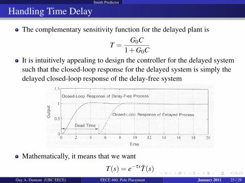
The complementary sensitivity function for the delayed plant is
T =G0C
1+G0CIt is intuitively appealing to design the controller for the delayed systemsuch that the closed-loop response for the delayed system is simply thedelayed closed-loop response of the delay-free system
Mathematically, it means that we want
T(s) = e−τsT(s)Guy A. Dumont (UBC EECE) EECE 460: Pole Placement January 2011 25 / 29

Smith Predictor
The Smith Predictor
The previous relationship between the two complementary sensitivitiesmeans
G0C1+G0C
= e−τs G0C1+ G0C
i.e.e−τsG0C
1+ e−τsG0C= e−τs G0C
1+ G0C
Solving for C yields
The Smith Predictor
C(s) =C
1+ G0C(1− e−τs)
Guy A. Dumont (UBC EECE) EECE 460: Pole Placement January 2011 26 / 29

Smith Predictor
The Smith Predictor
The Smith predictor corresponds to the structure below
Guy A. Dumont (UBC EECE) EECE 460: Pole Placement January 2011 27 / 29

Smith Predictor
The Smith Predictor
One cannot use the above architecture when the open loop plant isunstable. In the latter case, more sophisticated ideas are necessary.
There are significant robustness issues associated with this architecture.These will be discussed later.
Although the scheme appears somewhat ad-hoc, its structure is afundamental one, relating to the set of all possible stabilizing controllersfor the nominal system.
We will generalize this structure when covering the so-called Youlaparametrization or Q-design.
Guy A. Dumont (UBC EECE) EECE 460: Pole Placement January 2011 28 / 29
Smith Predictor
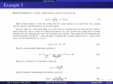
Example 5
Guy A. Dumont (UBC EECE) EECE 460: Pole Placement January 2011 29 / 29