ee578/4 #1spring 2008 © 2000-2008, richard a. stanley ece578: cryptography 4: more information...

EE578/4 #1Spring 2008© 2000-2008, Richard A. Stanley

ECE578: Cryptography

4: More Information Theory;

Linear Feedback Shift Registers

Professor Richard A. Stanley


Summary of last class...

• Probability plays an important role in cryptography, both in design and analysis

• Perfect secrecy can be achieved, but at great cost in key management– As a result, it is rarely attempted

• Using Shannon’s concept of entropy, we can provide an objective measure of information “leakage” through encryption

EE578/4 #3

Information Theory Revisited

• Shannon got his start in cryptography during World War II

• He applied much of what he had learned there to developing a mathematical model of communications, published soon after the war

• Most crypto information from WW II remained classified for many years

EE578/4 #4

Shannon’s Model of a Communications System

EE578/4 #5

Practical Considerations

EE578/4 #6

A Compression/Crypto Problem

EE578/4 #7

How About Now?

EE578/4 #8

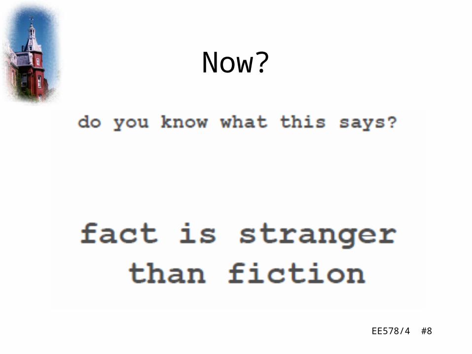
Now?

EE578/4 #9

Redundancy

• The sentence just presented is a very good example of what we mean by redundancy

• We are able to get the same information across to the audience without all of the letters and spaces in the sentence

• In our heads we can reconstruct the sentence• We have removed much redundancy

– This is akin to cryptography• Of course, there is a limit to what can be

removed ……

EE578/4 #10

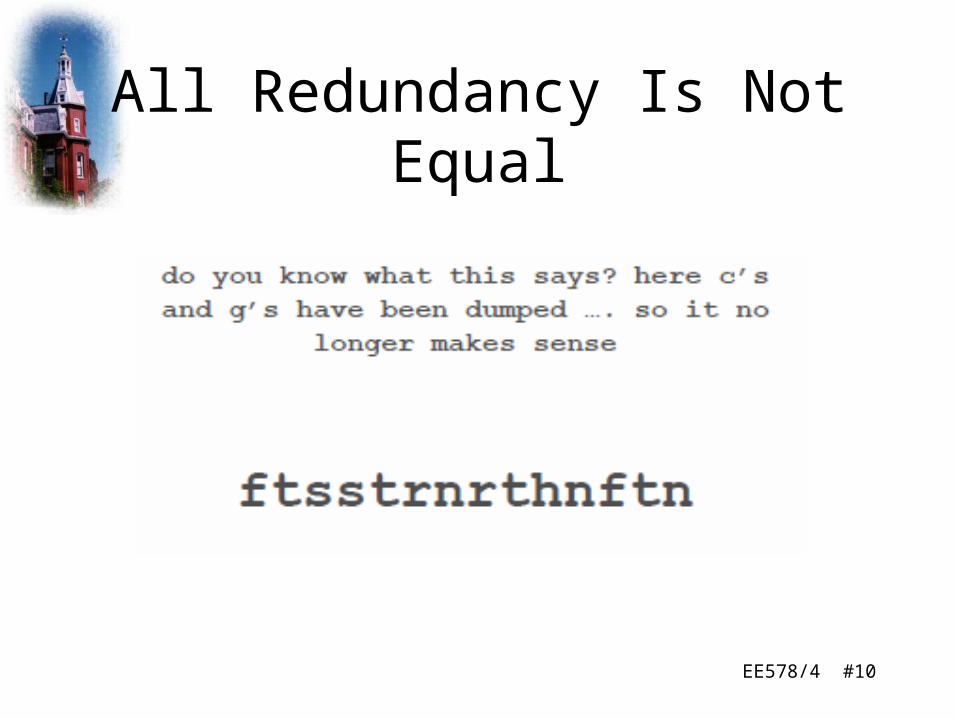
All Redundancy Is Not Equal

EE578/4 #11

Two Basic Questions

• What is the limit on how much compression can be applied while still being able to reconstruct the signal at the receiver?

• What is the maximum capacity of the channel in terms of information?

EE578/4 #12

Information Theory

EE578/4 #13

Information Theory

• We need to develop ideas about how to measure information to be able to answer the two questions set out above (how far can we compress something and how much information fits in the channel?)

• This is where information theory comes in– Information theory is a very general subject and not

just useful for mobile and wireless communications– Information theory grows from studies in

cryptography, and so applies there, too

EE578/4 #14

Essential Concepts

• Entropy

• Conditional Entropy

• Mutual Information

These concepts are fundamentalin information theory and will be used

in answering the two questions mentionedearlier.

EE578/4 #15

Uncertainty & Information

• Suppose we have a device that can produce 2 symbols, A, or B. As we wait for the next symbol, we are uncertain as to which symbol it will produce. How should uncertainty be measured? The simplest way would be to say that we have an “uncertainty of 2 symbols”.

• This would work well until we begin to watch a second device at the same time, which, let us imagine, produces 4 symbols *,~,% and &. The second device gives us an “uncertainty of 4 symbols” using the metric above.

• If we combine the devices into one device, there are eight possibilities, A*, A~, A%, A&, B*, B~, B% and B&. Using our metric this device has an “uncertainty of 8 symbols”.

EE578/4 #16

But…

• While it can be argued that this is a valid way of expressing the uncertainty it would be useful to be able to have a metric that was additive.

• We can think about measuring uncertainty as the log of the number of symbols, i.e. log (symbols)

• Logarithms have the kind of additive properties we are interested in.

EE578/4 #17

If We Think Logarithmically…

• We work in base two: log2 (symbols) as it is convenient for the digital world of 1’s and 0’s but would work in any base.

• So if the device produces 1 symbol we are uncertain by log2(1)=0

– i.e. we are not uncertain at all; we know what that symbol will be, because there is only one possibility

EE578/4 #18

Continuing…

• Using this notation we can say for device 1 (the device that produces A and B) we have an uncertainty of log2(2) = one bit.

• THINK DIGITAL: A may be represented by ‘1’ and B by ‘0’.

• We need only one bit to represent each symbol and our uncertainty as we wait for the symbol would be of the order 1 bit.

EE578/4 #19

If We Asked Binary Questions

• How many binary questions would we have to ask?

• The answer is 1– If we ask ‘is it 1?’ and the answer is

“yes” then it is a 1

– If the answer is “no” it is a 0

EE578/4 #20

Moving Right Along

• Using the logarithmic approach the uncertainty for device 2 is log2(4) = 2 bits.

• This makes some kind of intuitive sense, as we can represent our list of symbols *,~,%,& by 00,01,10,11 for example and as we wait for each symbol to arrive we have an uncertainty of two bits.

EE578/4 #21

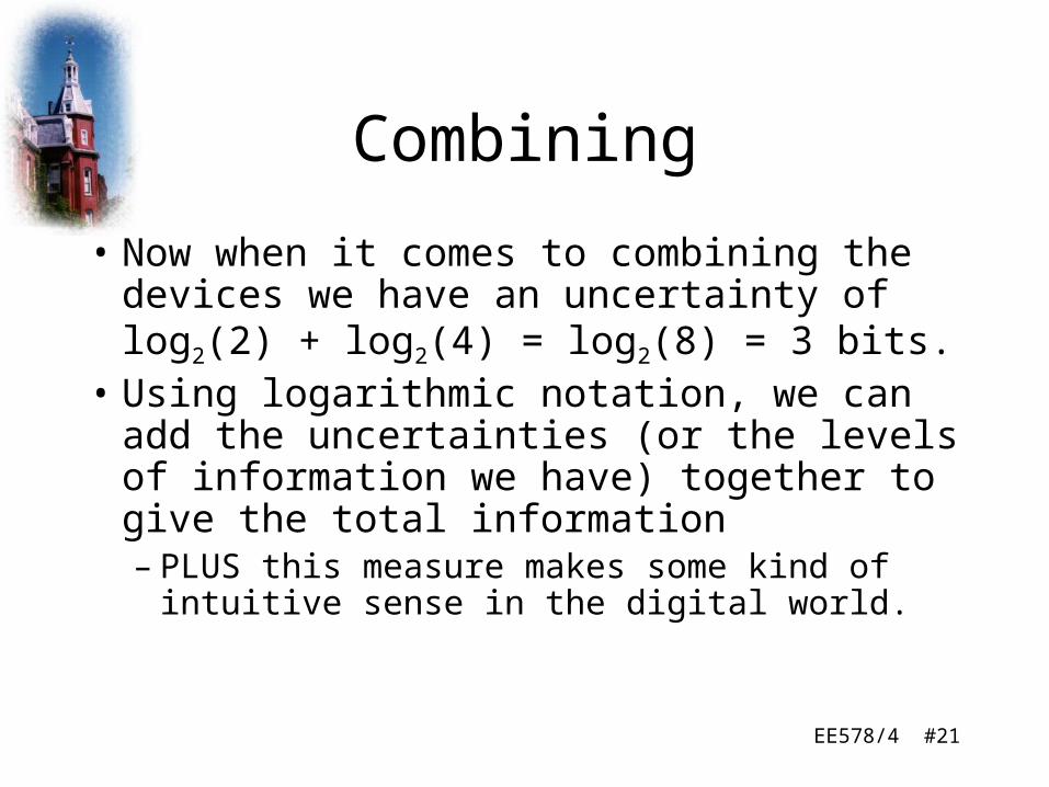
Combining

• Now when it comes to combining the devices we have an uncertainty of log2(2) + log2(4) = log2(8) = 3 bits.

• Using logarithmic notation, we can add the uncertainties (or the levels of information we have) together to give the total information– PLUS this measure makes some kind of

intuitive sense in the digital world.

EE578/4 #22

Moving Things Around

• So far we have used log2(symbols)– Let’s write this as log2(M) where M is the number of symbols– Assume each symbol is equiprobable (e.g. crypto)

• If we now rearrange our formula as follows• Uncertainty is now expressed in terms of P, the probability

that the symbol appears

EE578/4 #23

Back To the Two Devices

• We can use our simple devices to see that this is so

• Device 1 will output a random sequence of A’s and B’s

• It will produce A with a probability of 0.5 and B with a probability of 0.5 – as both are equally likely in a random sequence

• The uncertainty at the output of the device is given by –log2(0.5) = 1 bit as before

EE578/4 #24

Combinations of Devices

• The combined device produces a random sequence of 8 symbols, all equally likely.

• Hence each symbol has a probability of 1/8th and hence the uncertainty is given by –log2(0.125) which is 3 bits, as before

EE578/4 #25

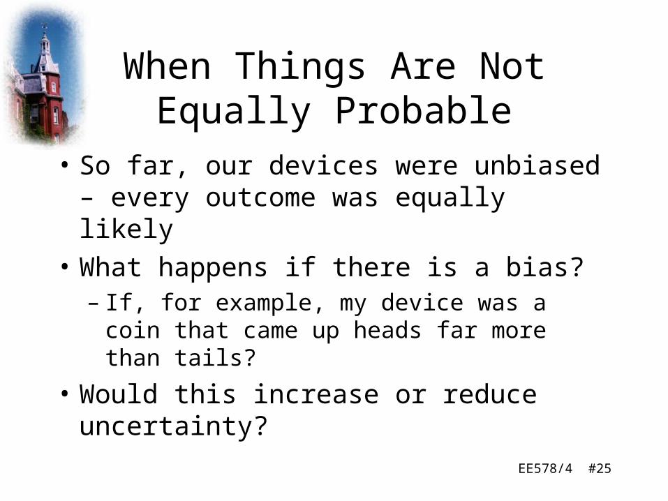
When Things Are Not Equally Probable

• So far, our devices were unbiased – every outcome was equally likely

• What happens if there is a bias?– If, for example, my device was a coin that came

up heads far more than tails?

• Would this increase or reduce uncertainty?

EE578/4 #26

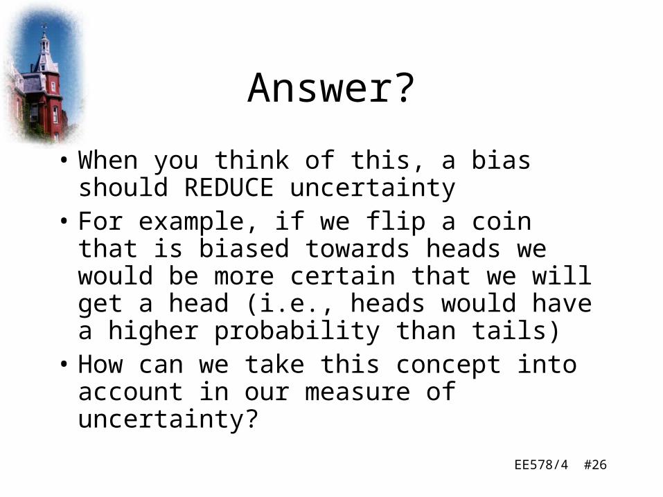
Answer?

• When you think of this, a bias should REDUCE uncertainty

• For example, if we flip a coin that is biased towards heads we would be more certain that we will get a head (i.e., heads would have a higher probability than tails)

• How can we take this concept into account in our measure of uncertainty?

EE578/4 #27

For Unequal Symbol Probabilities

• To get a measure of the uncertainty associated with the output of the device we need to sum the different uncertainties associated with each symbol, given that they are no longer equally probable

• We take a weighted sum of those uncertainties, the weights depending on the probability of each of the symbols

where Pi is the probability of the ith symbol from the alphabet of M symbols

EE578/4 #28

Thoughts

• The probabilities of each of the M symbols sum to 1– In other words, something must be sent

• If all symbols are equiprobable, this summation reduces to the simpler form we had earlier

EE578/4 #29

Shannon’s Entropy Equation

• The weighted sum of uncertainties over the alphabet of symbols is actually Shannon’s famous general formula for uncertainty.

• He used the term entropy to define this entity. It has the symbol H and we will use that from here on

• He came to this formula in a more rigorous manner – what we have done here is to more intuitively define the concept of entropy.

EE578/4 #30

Getting More Rigorous

• We will also now be more rigorous in our notation.

• X is a discrete random variable• X follows a probability distribution function P(x),

where x are the individual values in X, i.e., xX• We will speak of entropy H(X) – i.e. the entropy

of a discrete random variable• The random variable can the output of the devices

we spoke about earlier or any other random process we care to focus on

EE578/4 #31

Formal Definition• Let X be a discrete random variable which

takes on values from the finite set X. Then the entropy of random variable X is defined as the quantity

• Another logarithm base could be used; the adjustment is merely a constant factor

H(X) = – P[x] log2 P[x]xX

EE578/4 #32

Thinking About Entropy

• The entropy is a measure of the average uncertainty in the random variable

• It is the number of bits, on average, required to describe the random variable

• The entropy H of a random variable is a lower bound on the average length of the shortest description of the random variable – we have not shown this yet but this is one of Shannon’s famous deductions

EE578/4 #33

Sample Calculation 1

EE578/4 #34

Sample Calculation 2

EE578/4 #35

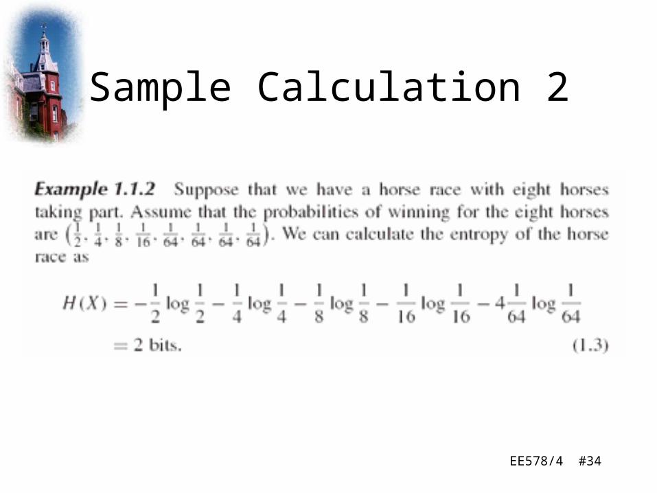
How Can It Be Only 2 Bits?

• If we go back to the idea that somehow the entropy gives a measure of the number of bits needed to represent the random variable how can we get two bits if there are eight entities in the race?

• If there are eight horses wouldn’t we need 3 bits per horse????

EE578/4 #36

Answer

• It is the average number of bits that the equation for entropy tells us

• So some random variables (horses in this case) can be represented by fewer than 3 bits while others can be represented by more than 3 bits

• The average turns out to be two

EE578/4 #37

More Details

• Suppose that we wish to send a message indicating which horse won the race

• One alternative is to send the index of the winning horse

• This description requires 3 bits for any of the horses

EE578/4 #38

But…

• The win probabilities are not uniform• It therefore makes sense to use shorter

descriptions for the more probable horses and longer descriptions for the less probable ones, so that we achieve a lower average description length.

• For example, we could use the following set of bit strings to represent the eight horses: 0, 10, 110, 1110, 111100, 111101, 111110, 111111

• The average description length in this case is 2 bits, as opposed to 3 bits for the uniform code

EE578/4 #39

A Graph of Entropy

EE578/4 #40

A Graph of Entropy - 2

EE578/4 #41

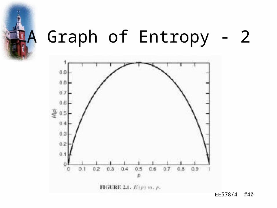
What Does This Tell Us?

• We get the sense the entropy relates to the information needed to convey the discrete random variable and that more information is needed when there is greater amounts of uncertainty

• Entropy is therefore a way of measuring information content

• In a two-symbol alphabet, maximum entropy occurs when the symbols are equiprobable

EE578/4 #42

So What?

• In channel coding, entropy gives a lower bound to the code length to represent symbols

• This, in turn, can be used to develop efficient codes, such as Huffman Codes– Entropy encoding algorithm for lossless data

compression

– Minimum redundancy code

– Based on probability of symbol occurrence

EE578/4 #43

Huffman Coding Example

• Designing a Huffman Code for the entire alphabet is not difficult, but it is tedious

• For illustration, we will only encode the 7 letters at left

Character Hexadecimal

Number of Occurences

(n) Percentage (p)

e 65 3320 30.5119

h 68 1458 13.3995

l 6C 1067 9.8061

o 6F 1749 16.0739

p 70 547 5.0271

t 74 2474 22.7369

w 77 266 2.4446

Total: 10881 100

EE578/4 #44

Huffman Coding Tree

Character Binary Code

e 0

h 11

l 110

o 10

p 1110

t 10

w 1111

EE578/4 #45

Entropy & Huffman Coding

• Entropy value gives a good estimate to the average length Huffman encoding, and vice versa

• Thus, the concept of entropy is not limited to cryptography, even though it began there


Some More Results From Information Theory

• Levels of Security– A cryptosystem is unconditionally secure if it cannot be

broken even with infinite computational resources

– A system is computationally secure if the best possible algorithm for breaking it requires N operations, where N is very large and known

– A system is relatively secure if its security relies on a well studied, very hard problem

• Example: A system S is secure as long as factoring of large integers is hard (this is believed to be true for RSA).


General Model of DES


Feistel Network in DES


Cryptography and Coding

• There are three basic forms of coding in modern communication systems: – source coding– channel coding– encryption

• From an information theoretical and practical point of view, the three forms of coding should be applied as shown on the next slide


Communication Coding System Model


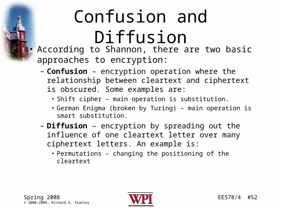
Confusion and Diffusion• According to Shannon, there are two basic approaches

to encryption:– Confusion – encryption operation where the relationship

between cleartext and ciphertext is obscured. Some examples are:

• Shift cipher – main operation is substitution.

• German Enigma (broken by Turing) – main operation is smart substitution.

– Diffusion – encryption by spreading out the influence of one cleartext letter over many ciphertext letters. An example is:

• Permutations – changing the positioning of the cleartext


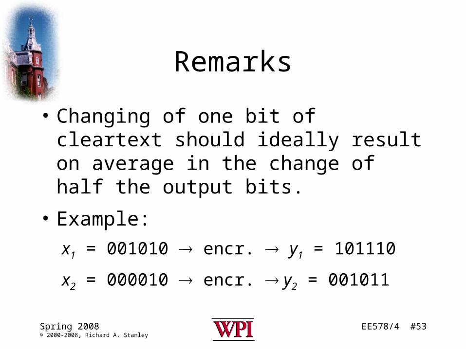
Remarks

• Changing of one bit of cleartext should ideally result on average in the change of half the output bits.

• Example:

x1 = 001010 encr. y1 = 101110

x2 = 000010 encr. y2 = 001011


Confusion + Diffusion

• Combining confusion with diffusion is a common practice for obtaining a secure scheme.

• The Data Encryption Standard (DES) is a good example of that

EE578/4 #55

Creating Keys

• For symmetric cryptosystems, we have seen that the ideal key is a random number string

• We have also seen that the logistics of providing such a key – especially with stream ciphers – are daunting

• Is there another way to produce the keys that is perhaps nearly as good as random numbers and that would simplify the logistics?

EE578/4 #56

D Flip-Flops

Input Outputs

S R D > Q Q'

0 1 X X 0 1

1 0 X X 1 0

1 1 X X 1 1

Output takes the value of the D input or Data input, and Delays it by maximum of

one clock pulse duration

EE578/4 #57

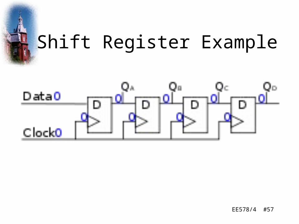
Shift Register Example


Linear Feedback Shift Registers (LFSR)

• An LFSR consists of m storage elements (flip-flops) and a feedback network. The feedback network computes the input for the “last” flip-flop as the XOR-sum of certain flip-flops in the shift register.– i.e. the input bit is a linear function of its

previous state• Example: We consider an LFSR of degree m = 3

with flip-flops K2, K1, K0, and a feedback path as shown on the next slide.


Why Do We Care?

• LFSR’s are used widely in cryptographic equipment to generate keys, and also to shift bits in the cryptographic algorithm

• Implementing these functions efficiently can have a considerable effect on the performance of the cryptographic engine


Linear Feedback Shift Register (LFSR) Example


LFSR Example Truth Table


LFSR Mathematics

• Mathematical description for keystream bits zi with z0, z1, z2 as initial settings:

z3 = z1 + z0 mod 2

z4 = z2 + z1 mod 2

z5 = z3 + z2 mod 2

• General case: zi+3 = zi+1 + zi mod 2 i = 0, 1, 2,...


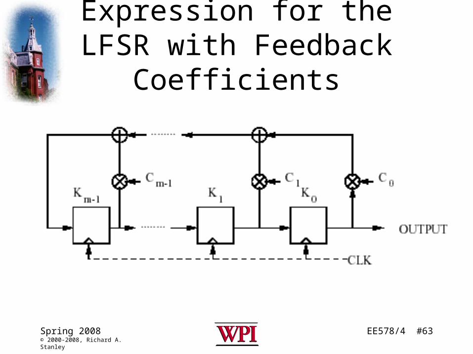
Expression for the LFSR with Feedback Coefficients


Feedback Coefficients

• C0, C1,..., Cm-1 are the feedback coefficients.

– Ci = 0 denotes an open switch (no connection)

– Ci = 1 denotes a closed switch (connection)

• zi+m = Cj zi+j mod 2; Cj {0,1}; i=0,1,2,...j=0

m-1


Key• The entire key consists of:

k= {(C0; C1; : : :; Cm-1),(z0,z1,...zm-1),m}

• Example: k={(1,1,0),(0,0,1),3}

• Theorem: The maximum sequence length generated by the LFSR is 2m-1– Proof: There are only 2 different states (k0...km) possible.

Since only the current state is known to the LFSR, after 2m clock cycles a repetition must occur. The all-zero state must be excluded since it repeats itself immediately.


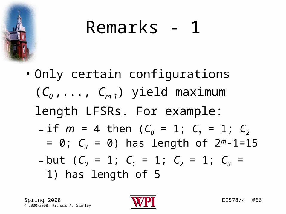
Remarks - 1

• Only certain configurations (C0 ,..., Cm-1)

yield maximum length LFSRs. For

example:

– if m = 4 then (C0 = 1; C1 = 1; C2 = 0; C3 = 0) has length of 2m-1=15

– but (C0 = 1; C1 = 1; C2 = 1; C3 = 1) has length of 5


Remarks - 2

• LFSRs are sometimes specified by polynomials such that P(x) = xm + Cm-1 xm-1 +...+ C1 x + C0

• Maximum length LFSRs have primitive polynomials

• These polynomials can be easily obtained from literature, for example(Co=1, C1=1, C2=0, C3=0,) P(x) = 1+x+x4


Primitive Polynomial

• Primitive polynomial of degree n:– Irreducible polynomial that

• divides x2n-1 +1

• does not divide xd+1 for any d that divides 2n-1

• No easy way to generate primitive polynomials mod 2– Easiest to generate polynomial and test it if is

primitive

EE578/4 #69

Some Polynomials for Maximal Length LFSRs

Fall 2008© 2000-2008, Richard A. Stanley

BitsFeedback polynomial

Period

n 2n − 1

4 x4 + x3 + 1 15

5 x5 + x3 + 1 31

6 x6 + x5 + 1 63

7 x7 + x6 + 1 127

8 x8 + x6 + x5 + x4 + 1 255

9 x9 + x5 + 1 511

10 x10 + x7 + 1 1023

11 x11 + x9 + 1 2047


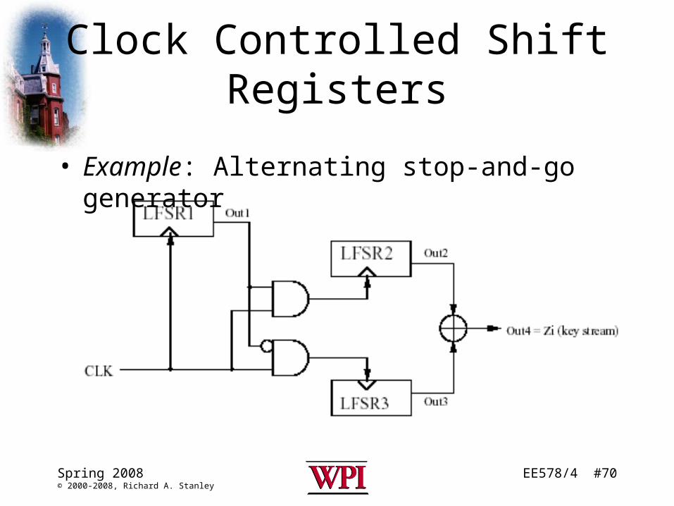
Clock Controlled Shift Registers

• Example: Alternating stop-and-go generator


Basic Operation

• When Out1 = 1 then LFSR2 is clocked; otherwise LFSR3 is clocked.

• Out4 serves as the keystream and is a bitwise XOR of the results from LFSR2 and LFSR3.


Security of the generator

• All three LFSRs should have maximum length conguration.

• If the sequence lengths of all LFSRs are relatively prime to each other, then the sequence length of the generator is the product of all three sequence lengths, i.e.,

L = L1 L2 L3


Security of the generator

• A secure generator should have LFSRs of roughly equal lengths and the length should be at least 128: m1 m2 m3 128

• Now, how could we attack the generator?


Known Plaintext Attack Against LFSRs

• For a known plaintext attack, we have to assume that m is known

• This attack is based on the knowledge of some plaintext and its corresponding ciphertext

– Known plaintext x0 , x1,..., x2m-1

– Observed ciphertext y0 , y1,..., y2m-1

– Construct keystream bits zi = xi + yi mod 2


Goal of the Attack

• To find the feedback coefficients Ci,by using the LFSR equation to find the Ci coefficients:


Solving the Equation



• Rewriting the equation in matrix form, we get:



• Solving for the Ci coefficients, we get


Attack Summary

• By observing 2m output bits of an LFSR of degree m and matching them to the known plaintext bits, the Ci coefficients can exactly be constructed by solving a system of linear equations of degree m

• LFSRs by themselves are extremely un-secure! – However, combinations of them such as the

alternating stop-and-go generator can be secure.

EE578/4 #80

Applications

• Very fast generation of a pseudo-random sequence, e.g. spread-spectrum comm.

• Counters

• PRNGs in cryptographic settings

• Digital communications, e.g. to prevent short repeating sequences (e.g., runs of 0's or 1's) from forming spectral lines

Spring 2008© 2000-2008, Richard A. Stanley


Summary

• Information theory provides important quantitative tools to measure effectiveness of cryptosystems

• LFSR’s are important components, widely used for key generation

• LFSR’s by themselves are not secure; however, combinations of LFSR’s can be made very secure


Homework

• Read Stinson, Chapter 1.2.5; reread Chapter 2• Problem 1: What is the pseudorandom sequence

generated by the linear shift feedback register (LFSR) characterized by (c2 = 1; c1 = 0; c0 = 1) starting with the initialization vector (z2 = 1; z1 = 0; z0 = 0)? What is the sequence generated from the initialization vector (z2 = 0; z1 = 1; z0 = 1). How are the two sequences related?


Problem 2• In this problem we will study LFSRs in somewhat more detail. LFSRs come in three

flavors– LFSRs which generate a maximum-length sequence. These LFSRs are based on primitive

• polynomials.– LFSRs which do not generate a maximum-length sequence but whose sequence length is

independent of the initial value of the register. These LFSRs are based on irreducible polynomials which are not primitive. Note that all primitive polynomials are also irreducible.

– LFSRs which do not generate a maximum-length sequence and whose sequence length depends on the initial values of the register. These LFSRs are based on reducible polynomials.

• We will study examples in the following. Determine all sequences generated by(a) x4 + x + 1(b) x4 + x2 + 1(c) x4 + x3 + x2 + x + 1

• Remember: The 1 coefficients of a polynomial give the feedback locations of the LFSR. Draw the corresponding LFSR for each of the three polynomials. Which of the polynomials is primitive, which is only irreducible, and which one is reducible? Note that the lengths of all sequences generated by a given LFSR should add up to 2m - 1.

ee578/4 #1spring 2008 © 2000-2008, richard a. stanley ece578: cryptography 4: more information...

Documents

information theory slide

uncertainty information

stanley slide

terms of information

crypto information

information fits

encryption slide

equal slide