ee571 digital communications i - kfupm
TRANSCRIPT

1/30/2014
1
EE571 Digital Communications I
Proakis Chapter 2Deterministic and Random Signal Analysis
Dr. Samir Alghadhban
1
Digital Communications System
2

1/30/2014
2
Why are Random Processes important?
• Random Variables and Processes let us talk about quantities and signals which are unknown in advance:
• The data sent through a communication system is modeled as random
• The noise, interference, and fading introduced by the channel can all be modeled as random processes
• Even the measure of performance (Probability of Bit Error) is expressed in terms of a probability.
3
Random Events
• When we conduct a random experiment, we can use set notation to describe possible outcomes.
• Example: Roll a six‐sided die.Possible Outcomes: S={1,2,3,4,5,6}
• An event is any subset of possible outcomes: A={1,2}
• The complementary event: • The set of all outcomes is the certain event: S• The null event: • Transmitting a data bit is also an experiment
4
A S A {3,4,5,6}

1/30/2014
3
Probability
• The probability P(A) is a number which measures the likelihood of the event A.
Axioms of Probability:
• No event has probability less than zero:
• Also and
• Let A and B be two events such that:
Then:
• All other laws of probability follow from these axioms
5
P(A) 0P(A) 1 P(A) 1 A S
A B P(A B) P(A) P(B)
Relationships Between Random Events
• Joint Probability: – Probability that both A and B occur
• Conditional Probability:
– Probability that A will occur given that B has occurred
• Statistical Independence:– Events A and B are statistically independent if:
– If A and B are independent then:
6
P(A, B) P(A B)
P(A B) P(A, B)
P(B)
P(A, B) P(A) P(B)
P(A B) P(A) and P(B A) P(B)

1/30/2014
4
Random Variables
• A random variable X(s) is a real‐valued function of the underlying event space:
• A random variable may be:– Discrete‐valued: range is finite (e.g. {0,1}) or countablyinfinite ( e.g., {1,2,3,...})
– Continuous‐valued ‐ range is uncountably infinite (e.g. )
• A random variable may be described by:– A name: X– It’s range: – A description of its distribution
7
X
s S
Probability Distribution Function (PDF)
8

1/30/2014
5
Probability Density Function (pdf)
9
Expected Values
10
1/30/2014
6
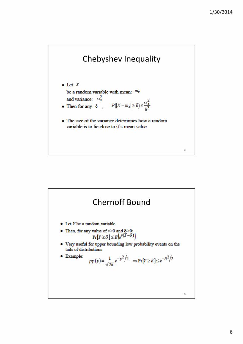
Chebyshev Inequality
11
Chernoff Bound
12

1/30/2014
7
Example #1: Uniform pdf
13
Example #1 (Find the mean and the variance)
14

1/30/2014
8
Example #2: Gaussian pdf
15
A Communication System with Gaussian Noise
16

1/30/2014
9
The Q‐function
17
The Q‐function and its Approximation
18

1/30/2014
10
Example #3 ‐ Rayleigh pdf
19
Rayleigh pdf
20

1/30/2014
11
Probability Mass Functions (pmf)
21
Example #1: Binary Distribution
22

1/30/2014
12
Example #2: Binomial Distribution
23
Example #2 (continued)
24

1/30/2014
13
Central Limit Theorem
25
Example of Central Limit Theorem:
26

1/30/2014
14
Random Processes
27
Terminology Describing Random Processes
28
1/30/2014
15
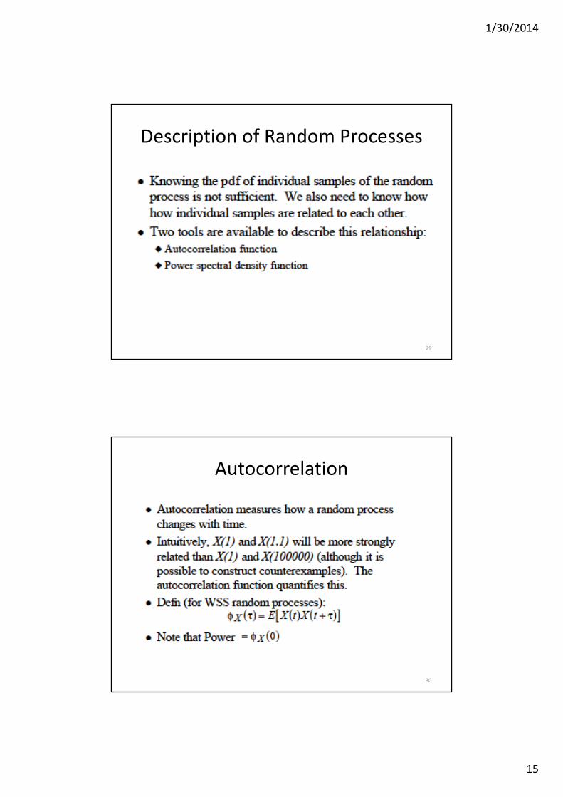
Description of Random Processes
29
Autocorrelation
30

1/30/2014
16
Power Spectral Density
31
Gaussian Random Processes
32
1/30/2014
17
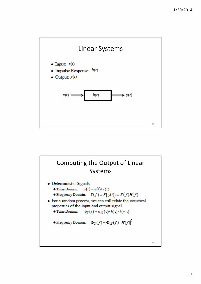
Linear Systems
33
Computing the Output of Linear Systems
34

1/30/2014
18
Gaussian Process
• Suppose that we observe a random process X(t) for an interval that starts at time t=0 and lasts until t=T.
• Suppose also that we weight the random process X(t) by some function g(t) and then integrate the product g(t)X(t) over this observation interval
• Thereby obtaining a random variable Y defined by:
• Y is a linear function of X(t)
35
Y g(t)X(t)o
T
dt
Gaussian Process
• If the mean‐square value of the random variable Y is finite and if the random variable Y is a Gaussian‐distributed random variable for every g(t) in this class of functions,
• Then the process X(t) is a Gaussian process
• In other words, the process X(t) is Gaussian process if every linear function of X(t) is a Gaussian random variable.
• For example,
36
Y ai Xii1
N

1/30/2014
19
Gaussian Process
• The random variable Y has a Gaussian distribution if its pdf is:
37
Where μY is the mean and σ2Y is the variance
The normalized Gaussian random variable Y has a zero mean (μY =0) and unit variance (σ
2Y =1) :
Normalized Gaussian distribution
38

1/30/2014
20
Gaussian Process
• A Gaussian process has two main virtues:
1‐ the Gaussian process has many properties that make analytic results possible
2‐ By experimental verifications, physical phenomena usually follow a Gaussian model.
39
Central Limit Theorem• The central limit theorem provides the mathematical justification for using a Gaussian process as a model for a large number of different physical phenomena in which the observed random variable, at a particular instant of time. is the result of a large number of individual random events.
• To formulate this important theorem, let Xi , i = 1, 2, . . . , N be a set of random variables that satisfies the following requirements:
1. The Xi are statistically independent.
2. The Xi have the same probability distribution with mean μX and variance σ
2X. 40

1/30/2014
21
Central Limit Theorem
• The Xi so described are said to constitute a set of independently and identically distributed (i.i.d.) random variables.
• Let these random variables be normalized as follows:
41
So that we have And
Define the new random variable
Central Limit Theorem
• The central limit theorem states that the probability distribution of VN approaches a normalized Gaussian distribution N(0, 1) in the limit as the number of random variables N approaches infinity.
42

1/30/2014
22
Properties of a Gaussian Process
Property 1:
• If a Gaussian process X(t) is applied to a stable linear filter, then the random process Y(t) developed at the output of the filet is also Gaussian.
43
Properties of a Gaussian Process
Property 2:• Consider the set of random variables or samples X(t1), X(t2), . .
., X(tn), obtained by observing a random process X(t) at times t1, t2, . . ., tn. If the process X(t) is Gaussian, then this set of random variables is jointly Gaussian for any n, with their n‐fold joint probability density function being completely determined by specifying
1‐ the set of means
2‐ and the set of covariance functions
44
1/30/2014
23
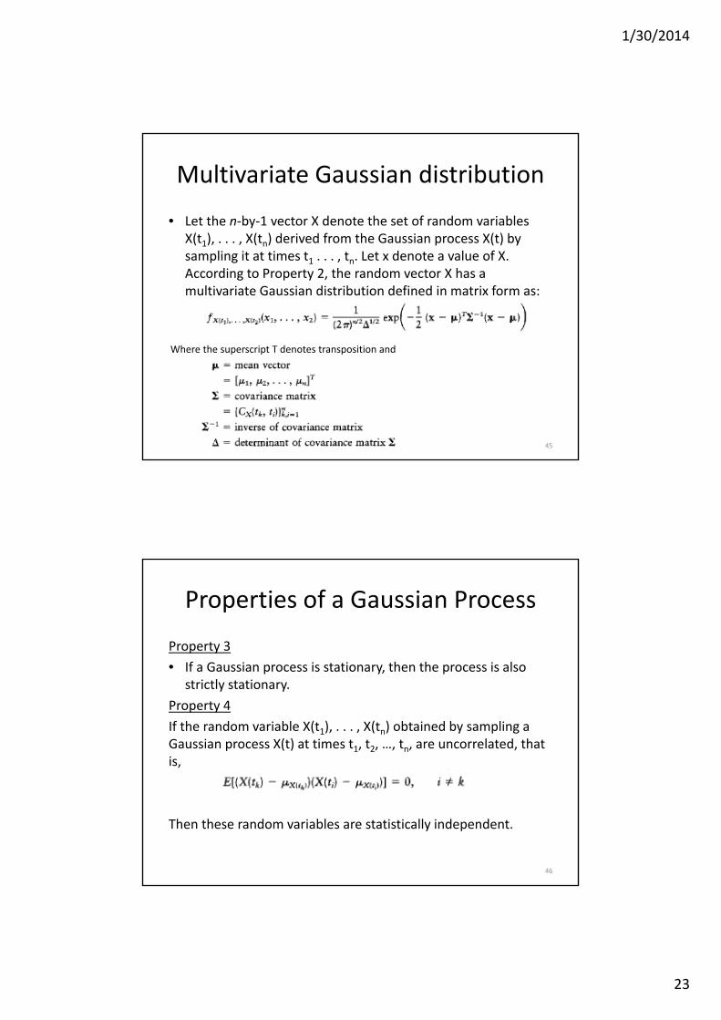
Multivariate Gaussian distribution
• Let the n‐by‐1 vector X denote the set of random variables X(t1), . . . , X(tn) derived from the Gaussian process X(t) by sampling it at times t1 . . . , tn. Let x denote a value of X. According to Property 2, the random vector X has a multivariate Gaussian distribution defined in matrix form as:
45
Where the superscript T denotes transposition and
Properties of a Gaussian Process
Property 3
• If a Gaussian process is stationary, then the process is also strictly stationary.
Property 4
If the random variable X(t1), . . . , X(tn) obtained by sampling a Gaussian process X(t) at times t1, t2, …, tn, are uncorrelated, that is,
Then these random variables are statistically independent.
46
1/30/2014
24
Properties of a Gaussian Process
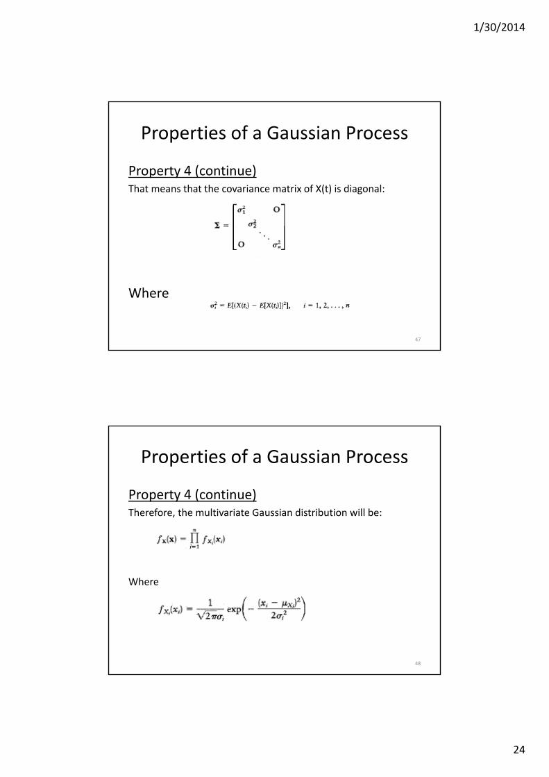
Property 4 (continue)That means that the covariance matrix of X(t) is diagonal:
Where
47
Properties of a Gaussian Process
Property 4 (continue)Therefore, the multivariate Gaussian distribution will be:
Where
48

1/30/2014
25
Properties of a Gaussian Process
Property 4 (continue)
In words, if the Gaussian random variables X(tl), . . ., X(tn) are uncorrelated., then they are statistically independent, which, in turn, means that the joint probability density function of this set of random variables can be expressed as the product of the probability density functions of the individual random variables in the set.
49
Noise
What do we mean by noise? From where does it come from? • The term noise is used customarily to designate unwanted signals that
tend to disturb the transmission and processing of signals in communication systems and over which we have incomplete control.
• There are many potential sources of noise in a communication system. – external to the system (e.g., atmospheric noise, galactic noise, man‐made
noise)– internal to the system, such as the noise that arises from spontaneous
fluctuations of current or voltage in electrical circuits. This type of noise represents a basic limitation on the transmission or detection of signals in communication systems involving the use of electronic devices.
• The two most common examples of spontaneous fluctuations in electrical circuits are shot noise anti thermal noise.
• White noise is an idealized form of noise used in communication systems analysis.
50

1/30/2014
26
Shot Noise
• Shot noise arises in electronic devices such as diodes and transistors because of the discrete nature of current flow in these devices.
• For example, in a photodetector circuit a current pulse is generated every time an electron is emitted by the cathode due to incident fight from a source of constant intensity.
• The electrons are naturally emitted at random timesdenoted by τk where ‐∞<k<∞
51
Shot Noise
• Thus, the total current flowing through the photo‐detector may be modeled as an infinite sum of current pulses as:
Where h(t‐ τk) is the current pulse generated at time τk
52

1/30/2014
27
Shot Noise
• The number of electrons, N(t), emitted in the time interval [0, t]constitutes a discrete stochastic process, the value of which increases by one each time an electron is emitted.
53
the mean value of the number of electrons, v, emitted between times t and t + ta is:
The parameter λ is a constant called the rate of the process. The total number of electronsemitted in the interval [t, t + t0] is:
Which follows a Poisson distribution with a mean value equal to
Shot Noise
The probability that k electrons are emitted in the interval [t, t + t0] is defined by:
54

1/30/2014
28
Thermal Noise
Thermal noise is the name given to the electrical noise arising from the random motion of electrons in a conductor.
The mean‐square value of the thermal noise voltage VTN appearing across the terminals of a resistor, measured in a bandwidth of ΔfHertz, is given by:
55
where k is Boltzmann's constant equal to 1.38 X 10‐23 joules per degree KelvinT is the absolute temperature in degrees Kelvin and R is the resistance in ohms
Noise Power
White Noise
• The noise analysis of communication systems is customarily based on an idealized form of noise called white noise, the power spectral density of which is independent of the operating frequency.
• The adjective white is used in the sense that white light contains equal amounts of all frequencies within the visible band of electromagnetic radiation.
• We express the power spectral density of white noise, with a sample function denoted by w(t), as
56

1/30/2014
29
White Noise
• The dimensions of N0 are in watts per Hertz.
• The parameter N0 is usually referenced to the input stage of the receiver of a communication system. It may be expressed as:
N0 = kTewhere k is Boltzmann's constant and Te is the equivalent noise temperature of the receiver
• The equivalent noise temperature of a system is defined as
the temperature at which a noisy resistor has to be maintained such that, by connecting the resistor to the input of a noiseless version of the system, it produces the same available noise power at the output of the system as that produced by all the sources of noise in the actual system
57
White Noise
Since the autocorrelation function is the inverse Fourier transform of the power spectral density, it follows that for white noise:
58
Strictly speaking, white noise has infinite average power and, as such, it is not physically realizable. Nevertheless, white noise has simple mathematical properties which make it useful in statistical system analysis.