ee-sunn chia p f p u c d p - princeton...
TRANSCRIPT
A CHEMICAL REACTION ENGINEERING PERSPECTIVE
OF POLYMER ELECTROLYTE MEMBRANE FUEL CELLS
Ee-Sunn Chia
A DISSERTATION
PRESENTED TO THE FACULTY
OF PRINCETON UNIVERSITY
IN CANDIDACY FOR THE DEGREE
OF DOCTOR OF PHILOSOPHY
2006

© Copyright by Ee-Sunn Chia, 2006.
All Rights Reserved
ii

iii
Acknowledgments I am tremendously grateful for the unsurpassable guidance I have received
throughout my entire graduate career from both my advisors Yannis and Jay. They have
continually guided me to be the engineer that I am today. The opportunity to work with
them simultaneously has been an invaluable learning experience.
My years in Princeton have flown by in the blink of the eye with friends that have
unfaltering energy to encourage and have fun. I’ll treasure the lunches, the dinners, the
game cube duels, our road trips, and the izakaya hopping. Many thanks to my closest
friends: Kat, Scott, Wanwipa, Phil, Daniel, Seachol, Sonia, Jason, and Mahdi. I’m also
thankful for wonderful labmates – both former and current Kevrekidis and Benziger
group members.
I am forever grateful for the support and motivation from my family. Although
hundreds and thousands of miles away, they were and are always just a phone call or an
email away. I owe it all to mom, dad, my brother Jason, and my sister Janice, for
inspiring me to get to where I am today.
Most importantly, I thank Lawrence for encouraging me throughout my academic
life from Virginia to Princeton. I am often in awe when I think about the confidence he
has instilled in me. Lawrence, thanks for being the patient listener, the exceptional
friend, and the caring husband.
Abstract
Polymer electrolyte membrane (PEM) fuel cells that are modeled and constructed
as a differential reactor enable an examination of the kinetics and dynamics associated
with the operating fuel cell. The differential reactor bypasses more complex two- and
three-dimensional integral reactors and simplifies the fuel cell to a one dimensional
system where spatial gradients are removed. The balance between water production and
water removal in the differential reactor gives rise to ignition/extinction phenomena and
multiple steady states. This phenomenon is a direct result of the polymer electrolyte
membrane’s role as a reservoir for water. A remarkable analogy between water balance
in the differential fuel PEM fuel cell and the energy balance in the classical exothermic
stirred tank reactor can be established.
In the initial chapters of this thesis, the rationale behind the design of the PEM
fuel cell as a differential reactor is described. A mathematical model of the PEM fuel cell
as a stirred tank which incorporates four of the key operating parameters: load resistance,
fuel cell temperature, inlet hydrogen flow rate, and inlet oxygen flow rate, successfully
captures the ignition/extinction phenomena. Changes in the water inventory as a result of
a change in any operating parameter will alter the membrane resistance. This affects the
rate of water production and ultimately will affect ignition/extinction.
In the later chapters of this thesis, the differential reactor is used as a building
block to model the integral type fuel cell reactors. The segmented anode parallel channel
PEM fuel cell was developed to provide insight into the inner workings of the fuel cell.
Specifically, this version of the fuel cell enabled individual current measurements within
iv

v
each segment which led to a spatial observation of the ignition front. A model of this
segmented anode parallel channel fuel cell based on coupled stirred tanks in series is also
presented at the end. In addition to the effects of the operating parameters on the fuel cell
operation, flow effects (co- and counter-current), and also configuration effects were
studied.

Contents
Abstract .............................................................................................................................. iv
1. Introduction and Overview ........................................................................................... 1
1.1 Obstacles to Fuel Cell Development..................................................................... 2
1.1.1 Hydrogen Production ................................................................................. 2
1.1.2 Hydrogen Storage ...................................................................................... 5
1.1.3 Cost ............................................................................................................ 6
1.1.4 Better Performance Fuel Cells ................................................................... 6
1.2 Our approach to PEM Fuel Cells .......................................................................... 7
2. A Brief Background of PEM Fuel Cells ..................................................................... 11
2.1 The Polymer Electrolyte Membrane (PEM) ....................................................... 11
2.2 The PEM Fuel Cell and its Components............................................................. 13
2.3 PEM Fuel Cell Modeling Efforts........................................................................ 17
3. The Differential PEM Fuel Cell.................................................................................. 22
3.1 The Stirred Tank Reactor PEM Fuel Cell........................................................... 22
3.2 Experimental Setup............................................................................................. 26
vi
3.3 System Variables and Parameters....................................................................... 28
3.4 Experimental Results .......................................................................................... 31
3.4.1 Fuel Cell Startup ...................................................................................... 31
3.4.2 Response to Changes in Operating Parameters ....................................... 36
3.4.3 Characteristic Times ................................................................................ 44
3.4.4 Polarization Curves.................................................................................. 45
3.4.5 Autonomous Oscillations......................................................................... 45
3.5 Summary ............................................................................................................. 47
4. Modeling Water Balance and Steady State Multiplicity in a STR-PEM fuel cell...... 50
4.1 Steady State Multiplicity..................................................................................... 51
4.2 The Simplified Stirred Tank Reactor PEM Model ............................................. 55
4.3 A Computational Parametric Study .................................................................... 67
4.4 Summary ............................................................................................................. 71
5. The STR-PEM Fuel Cell as a Reactor Building Block............................................... 73
5.1 Tanks in Series.................................................................................................... 73
5.2 The Segmented Anode Parallel Channel Fuel Cell............................................. 74
5.3 Current Evolution................................................................................................ 80
5.3.1 Ignition Fronts and Propagation............................................................... 82
5.3.2 Extinction Fronts...................................................................................... 87
5.4 Extended Operation Results................................................................................ 89
5.4.1 Polarization Curves.................................................................................. 89
5.4.2 Hydrogen Crossover Effect...................................................................... 93
5.4.3 Current Oscillations ................................................................................. 97
vii

5.5 Summary ............................................................................................................. 99
6. Modeling the Tanks in Series Fuel Cell.................................................................... 101
6.1 The Modified Stirred Tank Reactor PEM Model ............................................. 101
6.2 Flooding Effects at the Cathode........................................................................ 105
6.3 Mass Balances for the Stirred Tank Reactor PEM ........................................... 108
6.4 The Tanks in Series Model ............................................................................... 112
6.5 Results............................................................................................................... 113
6.5.1 The Single Stirred Tank Reactor........................................................... 113
6.5.2 Multiple STR-PEM fuel cells in series .................................................. 119
6.5.3 Computational Ignition Fronts............................................................... 123
6.6 Summary ........................................................................................................... 126
7. Conclusion ................................................................................................................ 128
References....................................................................................................................... 134
Appendix......................................................................................................................... 145
viii

List of Figures
1.0 Our PEM fuel cell research pathway ....................................................................... 3
2.1 The chemical structure of Nafion .......................................................................... 14
2.2 Schematic diagram of a typical PEM fuel cell....................................................... 14
2.3 Effect of low CO levels in the anode at T = 800C ................................................. 16
2.4 Schematic diagram of a gas diffusion electrode .................................................... 19
3.1 Visualizing the differential PEM fuel cell as a differential element from a
serpentine gas flow channel PEM fuel cell............................................................ 24
3.2 Comparing the serpentine flow channel to the mixed tank flow channel.............. 25
3.3 A schematic of the STR-PEM fuel cell experimental setup .................................. 27
3.4 Conceptual reactor coupling in the STR-PEM fuel cell ........................................ 30
3.5 Equivalent electrical circuit for the PEM fuel cell................................................. 32
3.6 Fuel cell startup from different initial water contents............................................ 34
3.7 Fuel cell startup with different load resistances..................................................... 35
3.8 Startup from different humidifier temperatures..................................................... 37
3.9 Fuel cell response to a step increase in temperature from 70°C to 90°C............... 38
ix

3.10 Fuel cell response to cooling from 90°C to 70°C .................................................. 40
3.11 Dynamic response to an increase in the external
load resistance from 20 Ω to 7 Ω ......................................................................... 41
3.12 Dynamic response to a change in the hydrogen feed
flow rate from 1 to 10 mL/min .............................................................................. 43
3.13 Polarization curves taken after the fuel cell was equilibrated at 80°C .................. 46
3.14 Autonomous oscillations observed in the STR-PEM fuel cell .............................. 48
3.15 Membrane swelling and relaxation are the likely
cause of the sustained oscillations ......................................................................... 48
4.1 Conductivity of a Nafion 115 membrane............................................................... 52
4.2 Steady state multiplicity in the STR-PEM fuel cell is analogous to the
classic steady state multiplicity in the exothermic CSTR...................................... 54
4.3 Humidification effect on the water balance in an STR-PEM fuel cell .................. 56
4.4 PEM fuel cell model .............................................................................................. 58
4.5 Predicting fuel cell startup with the simplified STR-PEM model ......................... 63
4.6 Water management and steady state multiplicity in a PEM fuel cell .................... 64
4.7 The Nafion 115 membrane resistance.................................................................... 66
4.8 Two-parameter bifurcation diagram in T and RL ................................................. 68
4.9 Two-parameter bifurcation diagram (a) T and nH2in (b) nO2
in and nH2in ................. 70
5.1 Schematic representation of several stirred tanks in series.................................... 75
5.2 The segmented anode parallel channel fuel cell .................................................... 77
5.3 Equivalent electrical circuit for the segmented anode fuel cell ............................. 79
5.4 The segmented anode fuel cell configuration ........................................................ 79
x

5.5 Current profiles in each segment over time for the fuel cell
equilibrated at room temperature ........................................................................... 81
5.6 Ignition fronts for a horizontally oriented flow channel fuel cell .......................... 84
5.7 Ignition fronts for the vertically oriented flow channel fuel cell ........................... 84
5.8 Total current profiles during ignition for the vertically oriented
fuel cell with reactants fed in: (a) counter-current; (b) co-current......................... 88
5.9 Extinction fronts..................................................................................................... 90
5.10a Overall power performance curve for the fuel cell ................................................ 92
5.10b Polarization curves for all six segments................................................................. 92
5.11 The external load resistance effect on current ....................................................... 95
5.12 The effect of decreasing the external load resistance on
the segmented anode fuel cell ................................................................................ 96
5.13 Autonomous oscillations observed for the horizontally
oriented parallel channel fuel cell with co-current flows....................................... 98
6.1 Water Transport Processes................................................................................... 103
6.2 Cathode GDL mass transfer................................................................................. 109
6.3 Building blocks .................................................................................................... 114
6.4 Flooding effects in the cathode ............................................................................ 116
6.5 Two-parameter bifurcation diagrams for the single
STR-PEM fuel cell with GDL flooding in: (a) T and RL; (b) T and FAin ........... 117
6.6 Two parameter bifurcation diagram for the single
STR-PEM fuel cell with GDL flooding in FAin and FC
in...................................... 118
6.7 Flooding Regions in Parameter Space ................................................................. 118
xi

6.8 Flow pattern effect on ignition for two STR-PEM fuel cells in series ................ 120
6.9 Transient current profiles for six tanks in co-current flow.................................. 122
6.10 Transient current profiles for six tanks in counter-current flow ......................... 122
6.11 Computed ignition fronts in a segmented anode
PEM fuel cell for co-current and counter-current flow ....................................... 124
xii

xiii
List of Tables
3.1 Relevant system variables and system parameters for
the STR-PEM the fuel cell. ...................................................................................... 32
3.2 Characteristic time constants that are associated with
various physical processes occurring in the PEM fuel cell...................................... 46
6.1 Relevant transport processes in the updated STR-PEM fuel cell model ............... 106

Chapter 1
Introduction and Overview
Although polymer electrolyte membrane (PEM) fuel cells have recently garnered
widespread attention as an alternative power source, they were actually developed over
forty years ago (Fuel Cell Handbook, 2000). In the early 1960s, PEM fuel cells devel-
oped by General Electric (GE) were used as a primary power source in Gemini space-
crafts. Unfortunately, both the lifetime and performance of PEM fuel cells were unsatis-
factory until DuPont introduced a perfluorosulfonic-acid membrane with a Teflon back-
bone, named Nafion™, in 1968. With the introduction of Nafion, cell performance im-
proved dramatically with power densities reaching 100 W/ft2 in 1970 and observed life-
times on the order of 103 hours (Watkins, 1993).
After the dramatic improvement brought forth by Nafion, other companies and
federal agencies such as United Technologies Corporation (UTC), Ballard Power Sys-
tems and Los Alamos National Laboratory (LANL) continued research in PEM fuel cells.
However, breakthroughs in PEM fuel cells were difficult due to the unreasonably high
costs associated with the catalyst and the membrane. Therefore, PEM fuel cells remained
1

largely unnoticed until Raistrick and his group at LANL discovered a method to impreg-
nate the gas diffusion electrodes with Nafion before hot pressing the electrodes onto the
membrane itself (Raistrick, 1986). This method led to a dramatic reduction in catalyst
requirements from 4 mg/cm2 of platinum to to 0.05 mg/cm2. This breakthrough in cata-
lyst reduction paved the way for more recent research in PEM fuel cells.
1.1 Obstacles to Fuel Cell Development
PEM fuel cells are extensively pursued for both mobile and stationary power ap-
plications (Fuel Cell Handbook, 2000; Acres, 2001; Perry and Fuller, 2002). More re-
cently, PEM fuel cells have become particularly attractive for automobile and mobile
electronic applications due to their relatively lightweight and compact construction in ad-
dition to their low operating temperature. However, researchers will need to address sev-
eral key issues in PEM fuel cell development before they will be able to mass produce
and market PEM fuel cells as a consumer product. Four main concerns in PEM fuel cell
development are discussed in what follows and are summarized in Figure 1.
1.1.1 Hydrogen Production
Concerns about the increased dependence on energy and exhausting the natural
nonrenewable fossil-fuels spurred interests in using hydrogen as a nonpolluting alterna-
tive. In 1973, Gregory presented a case to divert all energy sources towards hydrogen
production but research efforts in this area continue until today (Gregory, 1973). Hydro-
gen seems like a suitable fuel alternative since it is the most abundant element on earth
2

Figure 1: Our PEM fuel cell research pathway. We address the issue of PEM fuel cell performance by introducing a differential PEM fuel cell which enables us to focus on wa-ter management in the cell. In the later chapters, we will see that water is a variable that gives rise to complex nonlinear dynamical behavior reminiscent of classical exothermic stirred tank reactor dynamics. Through both experimental and modeling efforts, we iden-tify parameters that help us operate and optimize the fuel cell performance.
3

with an excellent energy density per weight. However, it is unfortunate that pure hydro-
gen sources are scarce; hydrogen is largely available in water and hydrocarbons.
The simplest method of hydrogen production is the electrolysis of water but the
electricity requirements make this an expensive route. A more common method of hy-
drogen production is steam reforming of natural gas which is followed by the water gas
shift reaction to remove carbon monoxide.
4 2 2
2 2
3CH H O H CO
CO H O H CO
+ → +
+ → + 2
Most of the hydrogen produced today is used for mainly two chemical processes:
ammonia production and fuel hydrocracking. Existing hydrogen production methods will
not generate enough hydrogen to meet the demands of a hydrogen economy. In a com-
mentary on hydrogen, Grant (Grant, 2003) estimates that 230,000 tonnes of hydrogen
need to be produced daily to sustain an economy dependent on fuel cell surface transpor-
tation. Grant also draws to attention the enormous number of new power plants required
to meet this requirement: 800 natural gas plants generating 500 MW which is equivalent
to 500 coal fired units (800 MW) or 200 Hoover Dams that generate 2 GW each. The
cost associated with constructing these new plants is undoubtedly a huge barrier. Some
also argue that splitting water to produce hydrogen creates as much greenhouse gas as
petroleum fuels (Grant, 2003; Washington, 2003).
In order to meet forecasted levels of hydrogen usage, newer methods of hydrogen
production are necessary. One such method is the autothermal reforming of ethanol to
produce hydrogen developed by Deluga et al. (Deluga et al., 2004). Hydrogen produc-
4

tion, directly or even indirectly, from biomass will aid in reducing greenhouse emissions
as well.
1.1.2 Hydrogen Storage
A breakthrough in hydrogen production will pave the way to a more realistic hy-
drogen economy but overcoming the hydrogen production problem alone is insufficient
because hydrogen storage remains an issue. Conventional storage methods in
tanks/cylinders are difficult to implement for gaseous hydrogen due to the extremely
large volume that gaseous hydrogen occupies. One solution is to pressurize the gas and
store it in specially designed tanks reinforced with carbon fibers. However, there are also
concerns that gaseous hydrogen is light enough to result in leakage from its storage me-
dium.
Another alternative is to liquefy the gaseous hydrogen and store it in insulated
double-walled vessels (Wolf, 2002). Since cryogenic liquid hydrogen boils at -252°C,
precautionary measures to minimize boil-off are necessary. The vessels used to store liq-
uid hydrogen are thus insulated with several layers. Newer methods of hydrogen storage
which are actively pursued include using various carbon forms: carbon nanotubes, inter-
calated plates, and carbon fibers (Baughman et al., 2002; Chambers et al., 1998; Dillon et
al., 1997; Liu et al., 1999). Crystalline metal organic frameworks that contain uniform
internal structure and size have also been suggested as possible media for hydrogen stor-
age (Rosi et al., 2003). Researchers have also used metals and alloys that can reversibly
absorb hydrogen, resulting in metal hydrides (Bogdanovic et al., 2000; Schlapbach and
Zuttel, 2001; Zaluski et al., 1997).
5

1.1.3 Cost
Most PEM fuel cells use a form of perfluorosulfonated acid membrane such as
Nafion (produced by DuPont). Unfortunately, the large cost of Nafion membranes is an-
other major impediment for commercial fuel cells. Therefore, alternative proton conduct-
ing membranes such as composite membranes (Liu et al., 2003; Nakajima and Honma,
2002; Yang, 2003) and hydrocarbon polymers are being developed (Kreuer, 2001; Riku-
kawa and Sanui, 2000). Aside from membrane cost alone, efforts to develop better and
cheaper electrodes also exist (Ralph et al., 1997). Further decrease in the platinum cata-
lyst loading requirements would help as well.
With any new technology, cost concerns are inevitable when it comes to develop-
ing a new hydrogen infrastructure to support the anticipated hydrogen demands for fuel
cells. As mentioned previously, hydrogen production and storage methods need to be
improved significantly before they are economically viable. For hydrogen production, a
suitable feedstock and production method will need to be discovered before hydrogen
becomes a competitive alternative to gasoline (Agrawal et al., 2005).
1.1.4 Better Performance Fuel Cells
Fuel cells for mobile applications will necessarily adjust to various non-steady
state requirements such as variable loads in power plants, climate effects on temperature
and humidity, and fast changes such as vehicle acceleration. The fuel cell performance
will need to be optimized for maximum power output under such changes. To develop
optimized fuel cells, three main issues need to be addressed: water management, heat
management, and catalyst poisoning.
6

Water management is a vital concern in PEM fuel cells because an optimum level
of water is necessary for the fuel cell to function. The membrane can only conduct the
protons if it is sufficiently humidified. However, too much water will result in flooding
that will create additional mass transport resistances for the reactants that are trying to
reach the catalyst.
Individual PEM fuel cells do not generate enough power for commercial applica-
tions. PEM fuel cells in practical applications will be produced in the form of fuel cell
stacks that will generate enough power (Amphlett et al., 1994; Chu and Jiang, 1999;
Hamelin et al., 2001; Lee and Lalk, 1998). Heat management is important when we con-
sider the heat dissipation from the fuel cell stacks.
Hydrogen sources that are reformed from hydrocarbon fuels often contain traces
of carbon monoxide that can poison the catalyst. Since current catalysts have very low
carbon monoxide tolerances, more robust catalysts need to be developed to withstand
such poisoning. Methods to generate cleaner hydrogen feeds must also be introduced.
1.2 Our Approach to PEM Fuel Cells
Before PEM fuel cells become a commercially viable alternative power source, it
is critical that predictive models of fuel cell performance for realistic operating conditions
are developed. Many PEM models attempt to capture the internal workings of an operat-
ing fuel cell (Bernardi and Verbrugge, 1992; Fuller and Newman, 1993; Janssen, 2001;
Pisani et al., 2002; Springer et al., 1991). However, such models often include intricate
details that create additional complexity. Predictive models of fuel cell performance that
7

correctly incorporate the transient interplay of reaction and transport processes are there-
fore critical.
Out of the four concerns highlighted above, we focus our research efforts in opti-
mizing the PEM fuel cell performance via a better understanding of what we believe is
the most interesting and controlling factor: water management. In this dissertation, we
apply fundamental reaction engineering knowledge to study a novel PEM fuel cell that
enables us to observe the effects of water on the fuel cell operation. We first review the
PEM fuel cell, its components, and provide an overview of PEM fuel cell modeling ef-
forts in Chapter 2.
In Chapter 3, we present the rationale behind our differential PEM fuel cell reac-
tor that was designed and constructed to examine kinetics and dynamics (Benziger et al.,
2005a; Benziger et al., submitted; Benziger et al., 2004; Benziger et al., 2005d). We
show that this differential reactor design, which bypasses the additional complexity of
two- and three-dimensional integral reactors (Bernardi and Verbrugge, 1992; Fuller and
Newman, 1993; Janssen, 2001; Springer et al., 1991) focuses on reaction/transport dy-
namic coupling under well-defined conditions. The differential PEM fuel cell (stirred
tank reactor (STR) PEM fuel cell) response is experimentally tracked as a function of the
controllable operating parameters: temperature, external load resistance, or hydrogen and
oxygen feed flow rates. Here, we also establish that the membrane functions as a reser-
voir for water in the fuel cell. This will be closely tied to the ignition/extinction phenom-
ena and multiple steady states that were reproducibly demonstrated by Moxley et al.
(Moxley et al., 2003). The experiments suggested that the proton transport dependence
on water activity in the PEM membrane underpins the observed dynamical phenomena.
8
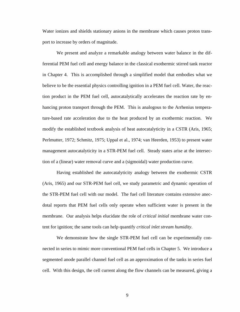
Water ionizes and shields stationary anions in the membrane which causes proton trans-
port to increase by orders of magnitude.
We present and analyze a remarkable analogy between water balance in the dif-
ferential PEM fuel cell and energy balance in the classical exothermic stirred tank reactor
in Chapter 4. This is accomplished through a simplified model that embodies what we
believe to be the essential physics controlling ignition in a PEM fuel cell. Water, the reac-
tion product in the PEM fuel cell, autocatalytically accelerates the reaction rate by en-
hancing proton transport through the PEM. This is analogous to the Arrhenius tempera-
ture-based rate acceleration due to the heat produced by an exothermic reaction. We
modify the established textbook analysis of heat autocatalyticity in a CSTR (Aris, 1965;
Perlmutter, 1972; Schmitz, 1975; Uppal et al., 1974; van Heerden, 1953) to present water
management autocatalyticity in a STR-PEM fuel cell. Steady states arise at the intersec-
tion of a (linear) water removal curve and a (sigmoidal) water production curve.
Having established the autocatalyticity analogy between the exothermic CSTR
(Aris, 1965) and our STR-PEM fuel cell, we study parametric and dynamic operation of
the STR-PEM fuel cell with our model. The fuel cell literature contains extensive anec-
dotal reports that PEM fuel cells only operate when sufficient water is present in the
membrane. Our analysis helps elucidate the role of critical initial membrane water con-
tent for ignition; the same tools can help quantify critical inlet stream humidity.
We demonstrate how the single STR-PEM fuel cell can be experimentally con-
nected in series to mimic more conventional PEM fuel cells in Chapter 5. We introduce a
segmented anode parallel channel fuel cell as an approximation of the tanks in series fuel
cell. With this design, the cell current along the flow channels can be measured, giving a
9

10
better idea of which portions of the fuel cell generate more current while allowing us to
observe ignition fronts in the cell.
In Chapter 6, we present a modified version of our initial STR-PEM fuel cell
model that incorporates key mass transport processes to capture flooding effects in the
cathode side catalyst/gas diffusion layer. We have employed our one-dimensional stirred
tank reactor model as a building block to model more complex flow geometries via a
“tanks-in-series” approach. This methodology provides a simplified straightforward ap-
proach to examine dynamics of PEM fuel cells. We have bypassed the more complex gas
diffusion layer models to be able to handle dynamics (Jeng et al., 2004; Lin et al., 2004;
Pasaogullari and Wang, 2004).

Chapter 2
A Brief Background of PEM Fuel Cells Ever since the introduction of the polymer electrolyte membrane (PEM) fuel cell by Wil-
liam Grubb (Grubb and Niedrach, 1960), researchers have been striving to incorporate
the PEM fuel cell technology into newer applications. This chapter begins with an over-
view of the PEM, followed by a brief background on PEM fuel cells. A description of
current fuel cell modeling efforts is presented at the end of this chapter.
2.1 The Polymer Electrolyte Membrane (PEM)
The PEM is a low density material with a relatively high mechanical strength,
making it suitable as an ion conductive gas barrier in fuel cells. The PEM exhibits desir-
able levels of oxygen solubility and proton conductivity while maintaining chemical sta-
bility (Srinivasan et al., 1993). PEMs have to operate at low temperatures to prevent
membrane dehydration since dry membranes exhibit decreased conductivity (Thampan et
al., 2000; Yang, 2003; Yang et al., 2004). Although there is interest in developing thin-
ner membranes for improved cell performance, this benefit is offset by the increased like-
11

lihood of reactant gas cross diffusion (Watkins, 1993) in addition to a loss of mechanical
strength.
DuPont’s introduction of a perfluorosulfonic-acid membrane known as Nafion
provided a significant improvement to previous hydrocarbon based membranes. Early
membranes consisted of polystyrene-divinylbenzene sulfonic acid crosslinked with an
inert fluorocarbon film. The C-H bonds in these early membranes had a tendency to de-
grade oxidatively, shortening the polymer lifetime in an operating fuel cell (Perry and
Fuller, 2002). As illustrated in Figure 2.1, Nafion differs from other membranes because
of its Teflon-like backbone. Nafion's inert properties in harsh conditions such as strong
acids or bases make it a suitable membrane in most applications. In a PEM fuel cell, the
Nafion membrane acts as a barrier to anions, allowing only the transport of cations (pro-
tons).
There are two well known models of the Nafion structure, one by Gierke and an-
other by Yeager. In the Gierke model, the ionic groups in Nafion aggregate and form
spherical clusters (connected by channels) that can swell with water (Eisenberg, 1970;
Gierke et al., 1981; Hsu and Gierke, 1982). Yeager offers a different view, suggesting
that Nafion consists of three different regions: a fluorocarbon phase, interfacial regions,
and ionic clusters (Yeager and Steck, 1981). Both models support the existence of ionic
clusters that have been shown to play an important role in the membrane water uptake.
Zawodzinski et al. showed that the membrane water uptake depends on the drying
method due to the ionic cluster reorganization during drying (Zawodzinski et al., 1993).
The membrane’s ability to absorb water is critical because proton conduction can
only occur when percolation pathways through the membrane are established. Therefore,
12
as mentioned previously, operating a PEM fuel cell at elevated temperatures will dry out
the membrane and result in decreased proton conductivity.
2.2 The PEM Fuel Cell and its Components
A typical PEM fuel cell consists of the anode, cathode, and the membrane electro-
lyte. Both electrodes contain platinum deposits to catalyze the reactions. Hydrogen fed
into the anode compartment is broken down into protons and electrons. The protons are
transported across the membrane to the cathode side, while the electrons travel via an ex-
ternal electrical circuit to the cathode. At the cathode, hydrogen and oxygen react to
form water. A schematic of the PEM fuel cell is shown in Figure 2.2.
Several factors that limit fuel cell performance include mass transfer limitations,
CO poisoning, and catalyst type. Mass transfer limitations arise from the transport of re-
actants to the electrodes in addition to the transport of protons across the membrane. Pro-
ton transport is only feasible when the membrane is sufficiently hydrated. As stated pre-
viously, a thinner membrane or a more ion-conductive membrane will enhance proton
transport into the cathode compartment.
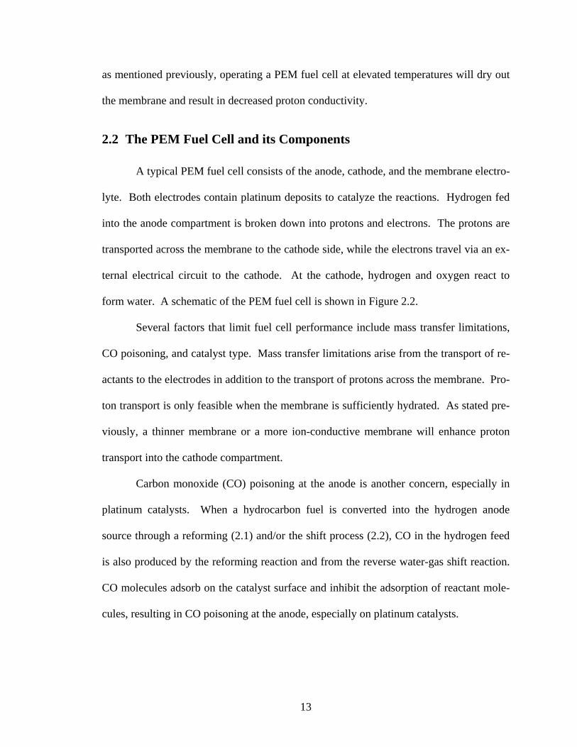
Carbon monoxide (CO) poisoning at the anode is another concern, especially in
platinum catalysts. When a hydrocarbon fuel is converted into the hydrogen anode
source through a reforming (2.1) and/or the shift process (2.2), CO in the hydrogen feed
is also produced by the reforming reaction and from the reverse water-gas shift reaction.
CO molecules adsorb on the catalyst surface and inhibit the adsorption of reactant mole-
cules, resulting in CO poisoning at the anode, especially on platinum catalysts.
13

Figure 2.1: The chemical structure of Nafion.
Inlet hydrogen
Anodeflow
channel
Cathodeflow
channel
H2O
H+
H+
(H2O)
(H2O)
Inlet oxygen
(H2O)H+
H2O
+→2H 2H+
=
=
→+ →
2
2
O 2OO 2H H O
Exit hydrogen Exit oxygen
Anode reactionCathode reaction
Inlet hydrogen
Anodeflow
channel
Cathodeflow
channel
H2O
(H2O)
(H2O)
H+
H+
Inlet oxygen
(H2O)H+
H2O
+→2H 2H+
=
=
→+ →
2
2
O 2OO 2H H O
Exit hydrogen Exit oxygen
Anode reactionCathode reaction
Figure 2.2: Schematic diagram of a typical PEM fuel cell. The membrane must remain sufficiently hydrated for proton transport.
14
(2.2)
(2.1) 3
222
224
HCOOHCO
HCOOHCH
+↔+
+↔+
Polarization effects (the loss of cell voltage due to current) are manifest in plots of cell
voltage as a function of current density. The polarization curves in Figure 2.3 depict the
effect of low CO levels in a PEM fuel cell at 800C as presented by Gottesfeld (Gottesfeld
and Pafford, 1988). Even low levels of CO significantly decrease the cell voltage, result-
ing in a smaller power output at a given current density; the presence of CO strongly in-
hibits fuel cell performance. Fortunately, CO levels may be reduced by injecting low
amounts of oxygen into the hydrogen anode feed stream. The added oxygen oxidizes the
adsorbed CO to CO2. However, a direct reaction between hydrogen and oxygen may also
occur, leading to a loss of fuel conversion (on the order of several percent).
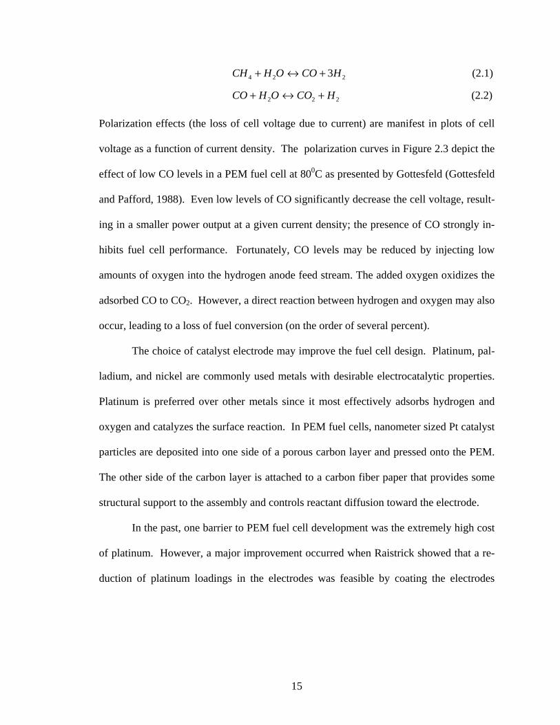
The choice of catalyst electrode may improve the fuel cell design. Platinum, pal-
ladium, and nickel are commonly used metals with desirable electrocatalytic properties.
Platinum is preferred over other metals since it most effectively adsorbs hydrogen and
oxygen and catalyzes the surface reaction. In PEM fuel cells, nanometer sized Pt catalyst
particles are deposited into one side of a porous carbon layer and pressed onto the PEM.
The other side of the carbon layer is attached to a carbon fiber paper that provides some
structural support to the assembly and controls reactant diffusion toward the electrode.
In the past, one barrier to PEM fuel cell development was the extremely high cost
of platinum. However, a major improvement occurred when Raistrick showed that a re-
duction of platinum loadings in the electrodes was feasible by coating the electrodes
15

Figure 2.3 Effect of low CO levels in the anode at T = 800C. Even ppm levels of CO significantly decrease the cell volt-age and result in a smaller power output at a given current density (Gottesfeld and Pafford, 1988).
16

with the perfluorinated ionomers in a liquid form (Raistrick, 1986). This step resulted in
an increased interfacial area since it created a thin layer of the polymer on the catalyst
before the hot pressing step. Since Raistrick’s important discovery, further refinements
in the area of membrane electrode assembly (MEA) preparation followed (Wilson et al.,
1993; Wilson and Gottesfeld, 1992). Flooding, which arises due to water condensation in
the pores can inhibit reactant diffusion toward the catalyst. The electrode contacting wa-
ter may be treated with a hydrophobic substance such as Teflon to prevent pore flooding
and wetting (Uchida et al., 1995).
2.3 PEM Fuel Cell Modeling Efforts
A fuel cell model is essential in optimizing fuel cell performance. An accurate
model will enable predictions of the cell performance under varied operating conditions.
Numerical and analytical fuel cell models that incorporate various aspects of heat, mass,
and momentum transport characteristics have been proposed in the past. Most modeling
efforts have focused on the various parts of the PEM fuel cell which include the gas dif-
fusion layer / gas flow channel (reactant transport), the polymer electrolyte membrane
(proton and water transport), and the catalyst layer (reaction site). Typical PEM fuel cell
models consist of transport equations for these respective parts and may include water
transport and heat effects.
Bernardi and Verbrugge initially developed a half-cell one-dimensional model of a
cathode gas diffusion electrode bonded to a fully hydrated polymer electrolyte membrane
under isothermal conditions (Bernardi and Verbrugge, 1991). As depicted in Figure 2.4,
the modeled system consists of the membrane region, an active catalyst layer, and a gas
17

diffusion layer. Corresponding transport equations were written for each respective layer.
Bernardi and Verbrugge later extended this model to a complete PEM fuel cell model
where they addressed limiting cell performance factors and mechanisms of species trans-
port within the PEM fuel cell (Bernardi and Verbrugge, 1992). Their work showed that
the membrane thickness and oxygen transport through the cathode to reaction sites affect
cell performance. Lower cell potentials were measured for thicker membranes while
higher limiting currents were obtained for more porous cathode electrodes. Prior to the
published work by Bernardi and Verbrugge mentioned above, Bernardi also proposed a
PEM fuel cell model based on gas phase transport which identified operating conditions
to ensure a water balance in the cell (Bernardi, 1990).
Elsewhere, Springer et al. presented a one dimensional steady-state model for a
complete PEM fuel cell with a Nafion membrane (Springer et al., 1991). This model was
used to address the issues of transport through porous electrodes and transport through
the membrane electrolyte by using calculated diffusivities (corrected for porosity) and
experimentally determined transport parameters. The model proposed by Springer et al.
does not require a fully hydrated membrane and thus differs from Bernardi and Ver-
brugge’s model.
When the protons migrate toward the cathode, water molecules are dragged by
osmotic action which creates a gradient in water concentration within the membrane, de-
pleting the anode side of water. Typically, water produced in the cathode reaction dif-
fuses back to the anode and the membrane remains hydrated. However, at high current
densities, water drag is more severe and it complicates the PEM fuel cell operation. In
the Springer model, water distribution in the fuel cell at steady-state is calculated by
18

Figure 2.4: Schematic diagram of a gas diffusion electrode. The modeled system consists of the membrane region, an ac-tive catalyst layer, and a gas diffusion layer (Bernardi and Ver-brugge, 1992).
19

accounting for water flow in the electrodes, membrane, and reactant inlets. Further re-
finements to incorporate interfacial kinetics at the catalyst/membrane interface, gas trans-
port, and conductivity issues were later proposed (Springer et al., 1993).
Two dimensional models of PEM fuel cells that address water management issues
have also been developed by several groups (Fuller and Newman, 1993; Gurau et al.,
1998; Hsing and Futerko, 2000; Nguyen and White, 1993). Fuller and Newman used
concentrated solution theory to model water transport and heat management in a two-
dimensional membrane electrode assembly (Fuller and Newman, 1993). Nguyen and
White focused on heat and mass transport along the gas flow channel while accounting
for water evaporation and condensation (Nguyen and White, 1993). In this work, they
obtained the temperature, water, gas and current density distribution in the gas flow
channels. This model did not account for the water variation across the membrane. The
parameters were determined from the anode side water content.
Gurau’s group sectioned the PEM fuel cell into three domains according to the
phases of the fluid (Gurau et al., 1998). The model was developed to closely describe the
species concentration distribution along the gas channel-gas diffusion-catalyst layer do-
main. This could only be accomplished by introducing two dimensional momentum
equations in the coupled domain. The transport, electrochemical, and current density
equations were then solved numerically to obtain polarization curves under various oper-
ating conditions. Hsing and Futerko presented a finite-element based model of coupled
fluid flow, mass transport, and electrochemistry (Hsing and Futerko, 2000). This model
was developed to operate without prior external humidification of the reactant gas. In a
later study, Gurau derived an analytical solution of a half-cell model for PEM fuel cells.
20

21
The ability to identify trends through functions instead of sets of numerical data was a
main incentive for developing the one-dimensional analytical model (Gurau et al., 2000).
Besides the transport models described above, electrochemical PEM fuel cell
models have been proposed. Mann et al. focused on developing a generalized steady-
state electrochemical model for a PEM fuel cell (Mann et al., 2000). Previous fuel cell
models were not applicable to cells with varying characteristics and dimensions. There-
fore, Mann's group developed a generic model that accepted operating variables and cell
parameters such as active area and membrane thickness. To account for the decrease in
the membrane's water-carrying capacity over time, the model also included a membrane
aging term. The model was only capable of predicting cell performance for an idealized
PEM cell utilizing Nafion.
In addition to other complete fuel cell models (Bevers et al., 1997; Pisani et al.,
2002; Springer et al., 2001; Standaert et al., 1996; Thirumalai and White, 1997), there
also exists a number of models that focus on water/proton transport within the membrane
(Janssen, 2001; Okada et al., 1998; Paddison, 2001), membrane/catalyst layer interface
(Eikerling and Kornyshev, 1998; Lin et al., 2004), and fuel cell stacks/systems (Amphlett
et al., 1994; Amphlett et al., 1998). Although many proposed models are capable of pre-
dicting experimental fuel cell performance, they are either too complicated or oversimpli-
fied. Most models can only predict the cell performance over limited operating condi-
tions. Therefore, the models do not yield an adequate fit of experimental data over all
conditions. Many models concentrate on either the entire cell or a half-cell that encom-
passes the membrane layer through the gas channel. Focusing on such a large region
makes it difficult to model the effects of various parameters within each layer.

Chapter 3
The Differential PEM Fuel Cell
Experimentally constructing and modeling the PEM fuel cell as a differential reactor al-
lows us to avoid the intricate details of water and proton transport through the PEM, elec-
tron transfer reactions at the electrodes, and transport through various layers of the fuel
cell. Most importantly, spatial and temporal variations are uncoupled in a differential
PEM fuel cell, enabling us to study the dynamics. We propose here a reaction engineer-
ing perspective of the PEM fuel cell as a differential reactor and describe the rationale
behind its design.
3.1 The Stirred Tank Reactor PEM Fuel Cell
PEM fuel cells consist of two graphite flow channels that sandwich a membrane
electrode assembly (MEA). Reactant gases are fed into the graphite flow channels, better
known as serpentine flow channels, typically contain tortuous pathways. Due to these
zigzag pathways, gradients in reactant concentration in both the anode and cathode flow
channels arise, causing a non-uniform current distribution over the membrane. While it
22

is feasible to track the current evolution over the membrane in both space and time, it
would be easier if one can focus on a differential element as illustrated in Figure 3.1.
Concentrating on such a small element allows one to assume that the reactant concentra-
tions are uniform in the anode and cathode chambers and that the only composition gra-
dient is transverse to the membrane. These well mixed chambers are the basis of the
stirred tank reactor (STR) PEM fuel cell (Benziger et al., 2004).
The characteristic dispersion number, a ratio of diffusive transport to convective
transport, provides a measure of mixing inside the flow channels. A characteristic dis-
persion number (D/uL) much larger than 1 indicates that diffusive transport dominates
and the gas phase is homogenous. Here, D is the diffusivity, L is the flow channel length
and u is the gas velocity. The GlobeTech serpentine flow field shown in Figure 3.2 con-
tains channels that are 100 mm in length with a cross sectional flow channel area of 1
mm2 over an MEA area of 5 cm2. In contrast, the flow channels in the STR-PEM fuel
cell are 14 mm in length with a cross section of 4 mm2 over a much smaller MEA area of
1 cm2. The dispersion number for the GlobeTech fuel cell producing 1.4 A/cm2 at 100%
H2 utilization with flow rates of 50 mL/min is less than 0.2. In comparison, for the STR-
PEM fuel cell producing the same current density with flow rates of 10 mL/min or less,
the dispersion number is greater than 1. Convective mixing in the serpentine flow field
thus creates compositional gradients along the flow channels.
Unlike typical PEM fuel cells, the STR-PEM fuel cell does not contain the tortu-
ous serpentine flow channels and it is operated at flow rates such that the gas phases in
the anode and cathode chambers remain well mixed (long residence times). The ho-
mogenous gas phase in the anode and cathode reduces the fuel cell to a one-dimensional
23

Figure 3.1: Visualizing the differential PEM fuel cell as a differential element from a serpentine gas flow channel PEM fuel cell. The schematic on the right is a blow up of the boxed element. In a serpentine type PEM fuel cell, variations in current density occur over the membrane. However, only gradients transverse to the membrane occur in a dif-ferential fuel cell.
24
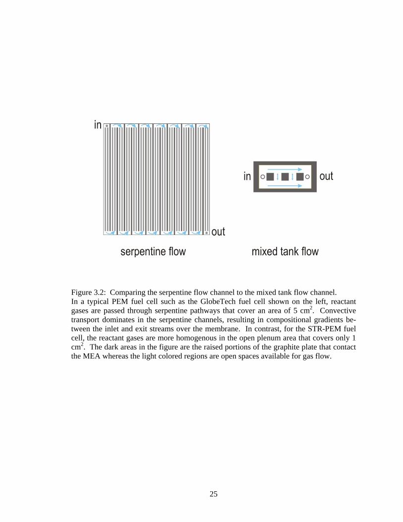
Figure 3.2: Comparing the serpentine flow channel to the mixed tank flow channel. In a typical PEM fuel cell such as the GlobeTech fuel cell shown on the left, reactant gases are passed through serpentine pathways that cover an area of 5 cm2. Convective transport dominates in the serpentine channels, resulting in compositional gradients be-tween the inlet and exit streams over the membrane. In contrast, for the STR-PEM fuel cell, the reactant gases are more homogenous in the open plenum area that covers only 1 cm2. The dark areas in the figure are the raised portions of the graphite plate that contact the MEA whereas the light colored regions are open spaces available for gas flow.
25

system which also significantly simplifies the data analysis. This unique chemical engi-
neering perspective of the PEM fuel cell as a stirred tank offers an important advantage in
studying the dynamics. We can address issues of fuel cell startup from different initial
conditions and whether or not the system parameters affect the fuel cell startup. Also, we
can study how the fuel cell responds to changes in the system parameters such as the load,
temperature, or reactant flow rates.
3.2 Experimental Setup
The first one-dimensional STR-PEM fuel cell system was constructed by previous
group members (Moxley et al., 2003) and we have also developed a mathematical model
of it (presented in the following chapter). There are four main parameters which an op-
erator can control: heat input to the cell (temperature), the variable external load resis-
tance, hydrogen flow rate into the anode, and oxygen flow rate into the cathode. The
STR-PEM fuel cell is connected to the variable load resistance. The current through and
the voltage drop across this load are measured. The experimental setup is schematically
illustrated in Figure 3.3.
The graphite plates with gas plenum volumes (V) of 0.2 mL contain machined pil-
lars that are matched between the two plates to ensure that pressure is applied uniformly
to the MEA. Hydrogen and oxygen gases are controlled through mass flow controllers
and fed at flow rates (Fin) between 1 and 10 mL/min. The residence times (V/Fin) of 1.2
to 12 s are longer than the characteristic diffusion times (V2/3/D) of 0.3 to 1 s. As men-
tioned previously, the residence times in the anode and cathode chambers are sufficiently
long so that the reactant gases remain well mixed.
26

Figure 3.3: A schematic of the STR-PEM fuel cell experimental setup. The STR-PEM fuel cell consists of two graphite plates that are sandwiching a membrane electrode assembly. The gas volumes above (anode chamber) and below the membrane (cathode chamber) are well mixed. The controllable parameters include the temperature, variable load resistance, and inlet reactant flow rates.
27
The MEA consists of a Nafion 115 membrane with an area of 1 cm2 that is hot
pressed between 2 E-tek electrodes with a catalyst loading of 0.4 mg Pt/cm2. The E-tek
electrodes are carbon cloths that come coated with a Pt/C catalyst. The electrodes are
impregnated with a 5% Nafion solution to a loading of 0.6 mg/cm2 before hot pressing
with a 2200 lbf (9.77 kN) at 130°C. The MEA is then placed between two silicon rubber
gaskets before it is sandwiched between the graphite plates. Copper sheets are pressed
against the graphite plates with wires that attach to the external variable load resistor.
The graphite plates are placed in between aluminum blocks that are fitted with cartridge
heaters connected to a temperature controller.
A 10 turn 0 to 20 Ω potentiometer is used as the variable external load resistor.
Current through the load resistor is also passed through a 0.2 Ω sensing resistor and an
instrumentation amplifier (Analog Devices AMP02) amplifies the differential voltage
across the sensing resistor by a factor of 100. The current is read directly by a data ac-
quisition board.
3.3 System Variables and Parameters
It is important to identify the system variables from the system parameters before
proceeding to the experimental results. The system variables in the STR-PEM fuel cell
system are quantities that describe the local state of the fuel cell and these quantities can-
not be directly controlled. However, the system parameters are quantities that an opera-
tor can manually change based on his/her discretion. For instance, one can regulate the
amount of water fed into the fuel cell but the membrane water content is a measurable
quantity that cannot be directly controlled. The membrane water content (as indicated by
28

the membrane water activity aw) depends on many factors including the rate of water
production (as indicated by the current), the inlet water content (water fed), and exiting
water content (water removed), as well as the cell temperature. Since the operator cannot
directly fix the membrane water content, it is an example of a system variable. We will
later show that the membrane water content is an important variable that is responsible
for the unique dynamics characteristic of the STR-PEM fuel cell.
We have chosen to operate the STR-PEM fuel cell under a fixed external load re-
sistance (a system parameter) and we let the voltage and the current evolve. The voltage
and the current are system variables that depend on the membrane water content. Since
we neither fix the voltage nor the current, the STR-PEM fuel cell is not potentiostatically
or galvanostatically regulated. We have chosen to operate the fuel cell this way so that
we may study the autonomous response to the four operating parameters. If we choose to
control the voltage or current, implementing a potentiostatic or galvanostatic control loop
on the fuel cell system would prevent us from extracting information pertaining to the
kinetics of the operating fuel cell.
The STR-PEM fuel cell can be schematically depicted as two reactors (anode and
cathode) that are connected by two valves as shown in Figure 3.4. The two valves repre-
sent the external load resistance (RL, a system parameter) that regulates the electron flow
across the external circuit and the membrane resistance (RM, a system variable) that regu-
lates the proton flow across the membrane. RM is not directly controllable because it has
been shown to be strongly dependent on the water content in the membrane (membrane
water activity) (Yang, 2003). In addition to RL, inputs to the fuel cell such as the feed
composition and feed flow rates are system parameters. On the other hand, the
29

Figure 3.4: Conceptual reactor coupling in the STR-PEM fuel cell. Inputs that lie out-side of the dashed box are directly controllable operating parameters. The external load resistance and the membrane resistance act as valves that regulate the electron flow across the external circuit and the proton flow across the membrane respectively.
30

exiting flow rates and effluent composition are system variables since these quantities
depend on the mass balance between reaction and production in the fuel cell. An opera-
tor can only control the parameters that lie outside of the dashed box which represents the
physical boundary of the fuel cell. Note that the two regulators are connected in series,
indicating that the total resistance is the sum of both resistances.
From the electrical circuit equivalent of the fuel cell as shown in Figure 3.5, the
current is defined according to Ohm’s law as:
M L
ViR R
=+
(3.1)
Therefore any increase in RM or RL will result in a lower overall current. A list of the sys-
tem parameters and variables is shown in Table 3.1.
3.4 Experimental Results
3.4.1 Fuel Cell Startup We are particularly interested in the fuel cell startup behavior from different ini-
tial conditions. In a previous experiment, the importance of an optimum level of water in
the fuel cell was illustrated (Benziger et al., 2004). The membrane was first dried by
flowing dry nitrogen gas through the anode chamber and dry oxygen gas through the
cathode chamber at flow rates of 100 mL/min for 12 hrs while maintaining the cell tem-
perature at 60°C. The membrane was then preconditioned to a fixed humidification level
by shutting off the oxygen flow to the cathode and passing 10 mL/min of nitrogen gas
through a water bubbler (equilibrated at room temperature) before it was fed into the an-
ode chamber. The anode effluent relative humidity was measured as a function of time to
31

Figure 3.5: Equivalent electrical circuit for the PEM fuel cell. Both resistances are connected electrically in series so that any increase in either resistance will lead to a decreased cell current. The membrane resistance is a strong function of the membrane water content (activ-ity).
System Variables System Parameters Effluent flow rates Reactant feed flow rates Effluent composition Reactant feed composition Gas relative humidity Membrane material Cell temperature Heat Input Cell voltage Cell construction Cell current Electrode structure Membrane water content External Load Resistance
Table 3.1: Relevant system variables and system parame-ters for the STR-PEM the fuel cell.
32
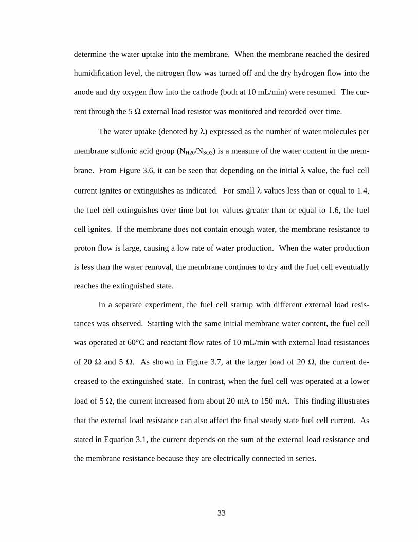
determine the water uptake into the membrane. When the membrane reached the desired
humidification level, the nitrogen flow was turned off and the dry hydrogen flow into the
anode and dry oxygen flow into the cathode (both at 10 mL/min) were resumed. The cur-
rent through the 5 Ω external load resistor was monitored and recorded over time.
The water uptake (denoted by λ) expressed as the number of water molecules per
membrane sulfonic acid group (NH20/NSO3) is a measure of the water content in the mem-
brane. From Figure 3.6, it can be seen that depending on the initial λ value, the fuel cell
current ignites or extinguishes as indicated. For small λ values less than or equal to 1.4,
the fuel cell extinguishes over time but for values greater than or equal to 1.6, the fuel
cell ignites. If the membrane does not contain enough water, the membrane resistance to
proton flow is large, causing a low rate of water production. When the water production
is less than the water removal, the membrane continues to dry and the fuel cell eventually
reaches the extinguished state.
In a separate experiment, the fuel cell startup with different external load resis-
tances was observed. Starting with the same initial membrane water content, the fuel cell
was operated at 60°C and reactant flow rates of 10 mL/min with external load resistances
of 20 Ω and 5 Ω. As shown in Figure 3.7, at the larger load of 20 Ω, the current de-
creased to the extinguished state. In contrast, when the fuel cell was operated at a lower
load of 5 Ω, the current increased from about 20 mA to 150 mA. This finding illustrates
that the external load resistance can also affect the final steady state fuel cell current. As
stated in Equation 3.1, the current depends on the sum of the external load resistance and
the membrane resistance because they are electrically connected in series.
33
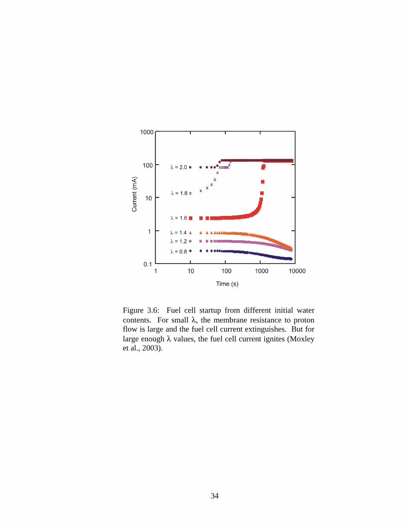
Figure 3.6: Fuel cell startup from different initial water contents. For small λ, the membrane resistance to proton flow is large and the fuel cell current extinguishes. But for large enough λ values, the fuel cell current ignites (Moxley et al., 2003).
34

Figure 3.7: Fuel cell startup with different load resistances. The larger external load resistance of 30 Ω suppresses the water production rates, resulting in a drier membrane which eventually leads to the current extinguishing. In contrast, the fuel cell starting up from 5 Ω is able to balance the water removal and water production rates and ultimately reaches the ignited current steady state (Benziger et al., 2004).
35

Besides the initial membrane water content and external load resistance, the inlet
reactant humidification levels also affect startup. To test the humidification effects, the
membrane was first dehydrated by flowing dry gases into the anode and cathode for 12
hours at 60°C. A dry oxygen supply was then fed to the cathode while the hydrogen feed
was passed through a bubbler operating at 25°C. Both reactant feeds were set to 10
mL/min. Figure 3.8 shows that increasing the humidifier temperature from 25°C to 30°C
led to the fuel cell current igniting to about 80 mA after 1000 s. When the anode stream
was further humidified by increasing the bubbler temperature to 35°C, ignition occurred
even earlier and the high current steady state was reached after about only 300 s. From
this result, we see that while the feed humidification levels affect the time to ignition, the
final steady state current depends predominantly on the membrane water content.
3.4.2 Response to Changes in Operating Parameters
A real fuel cell operating in practical applications will necessarily respond to
various heating conditions, external load demands, and fuel supply limitations. As an
initial step, the fuel cell response to changes in several operating parameters was studied
to get a better insight of the fuel cell dynamics. The fuel cell response to a change in the
cell temperature, external load resistance, and hydrogen flow rate was monitored.
In one experiment, the reactant flow rates and the external load were held at 10
mL/min and 2 Ω respectively and the voltage, current, and effluent relative humidity re-
sponse to an increase in the fuel cell temperature from 70°C to 90°C were observed. The
cell temperature reached 90°C in about 200 s but the cell current took slightly longer to
equilibrate. The current response as depicted in Figure 3.9 is seen to initially decrease
36

Figure 3.8: Startup from different humidifier temperatures. While feeding a dry oxygen supply to the cathode, the hydrogen feed was passed through a bubbler (held at different temperatures) before be-ing fed into the anode. Heating the bubbler temperature to 30°C in-creased the water content in the anode feed, leading to the current igniting. Further humidification (bubbler temperature at 35°C) shortened the ignition time.
37

Figure 3.9: Fuel cell response to a step increase in temperature from 70°C to 90°C with the external load resistance at 2 Ω and reactant feed flow rates of 10 mL/min. A decrease in fuel cell current was observed as a result of the larger rate of water removal.
38
with heating from 78 mA to 45 mA but subsequently equilibrates at 65 mA. The heating
process increased the water vapor pressure which resulted in a greater rate of water re-
moval. The early decline in current is thus attributed to the water evaporation from the
membrane which was initially faster than the diffusion of water in the membrane. Over
time, water in the membrane and water in the membrane-electrode interfaces equilibrate
and a final steady state is reached. The effluent cathode and anode relative humidities
decrease with the higher temperature as well.
Cooling the fuel cell from 90°C to 70°C was accompanied by an increase in cell
current from 61 mA to 83 mA as shown in Figure 3.10. Note that the cooling process
took longer than the heating since it is a passive process. Both the cathode and anode
relative humidities increased with the temperature drop, indicating that less water is re-
moved due to a decrease in water vapor pressure. The lower rate of water removal led to
an increased membrane water activity. As mentioned previously, the membrane resis-
tance is lower at a larger membrane water activity, resulting in a larger fuel cell current.
For both the heating and cooling processes, the complex coupling between the water pro-
duction at the cathode and water transport across the membrane results in differences in
the anode and cathode relative humidity responses.
The fuel cell response to a change in the external load resistance was observed by
decreasing the external load resistance from 20 Ω to 7 Ω. Prior to this change, the fuel
cell was set to operate at 80°C with 5 mL/min of H2 flow to the anode and 10 mL/min of
O2 flow to the cathode. From Figure 3.11, it can be seen that the dynamic response to the
decrease in the load resistance was rather unusual. The cell current immediately in-
creased from 25 mA to about 76 mA before it gradually decayed to 65 mA. Despite
39

Figure 3.10: Fuel cell response to cooling from 90°C to 70°C with the external load resistance at 2 Ω and reactant feed flow rates of 10 mL/min. Less water is removed at the lower temperature, leading to a lower membrane resistance which resulted in an increase in the cell current.
40

Figure 3.11: Dynamic response to an increase in the external load resistance from 20 Ω to 7 Ω at a fixed temperature of 80°C with 5 mL/min of H2 flow to the anode and 10 mL/min of O2 flow to the cathode. The cell current first rises rapidly before reaching a pla-teau at 65 mA but subsequently makes another jump to 84 mA after 1500 s. The cathode relative humidity tracks the current while the anode relative humidity lags that of the cathode.
41

leveling out at 65 mA, the cell current subsequently jumped to 84 mA after 1500 s (with-
out any change in the operating parameters). The anode relative humidity response is
seen to lag that of the cathode relative humidity response by about 100 s.
To observe the dynamic response to a change in the hydrogen feed, the fuel cell
was first operated at 80°C and 2 Ω with 10 mL/min of O2 flow to the cathode and 1
mL/min of H2 flow to the anode for 12 hours. The H2 flow was then increased up to 10
mL/min and the current, voltage, and effluent relative humidity responses were tracked.
Immediately following the change in H2 flow, as shown in Figure 3.12, the current in-
creased from 3 to 80 mA over 10 s. The current kept increasing but at a slower rate to
100 mA, and subsequently jumped to 145 mA after 650 s.
The initial increase in current is caused by the sudden increase in the hydrogen
supply. After that initial response, the fuel cell took some time to adjust to the increased
water production rates and equilibrated to the plateau. The surprising jump in current is
most likely the result of the balance between water transport in the membrane and the
mechanical stress relaxation. We believe that the membrane swells with the increased
water production and improves the membrane electrode contact, thereby resulting in a
sudden jump in the current.
The cathode relative humidity is seen to track the current (by about 10 seconds)
while the anode relative humidity tracks the cathode relative humidity. As the current
increased slowly to 100 mA, the cathode relative humidity increased significantly as well
from 45% to 85% but slowed down when then current jumped. The anode relative hu-
midity increased by 10% from 35%. These increased effluent relative humidities are the
result of the increased water production rates.
42

Figure 3.12: Dynamic response to a change in the hydrogen feed flow rate from 1 to 10 mL/min for a fuel cell equilibrated at 80°C, 2 Ω external load, 10 mL/min of oxygen fed to the cath-ode, and 1 mL/min of hydrogen supplied to the anode. Follow-ing the initial increase in current, the fuel cell equilibrated to the new conditions over 600 seconds.
3.4.3
43

Characteristic Times From the observed responses to changes in operating parameters, it is evident that
there are characteristic times associated with physical processes in the fuel cell. Contrary
to the common assumption that PEM fuel cell response times are almost instantaneous,
we have shown that the response times can take as long as hundreds of seconds. Several
characteristic time constants can be derived for the fuel cell and they are listed in Table
3.2 along with order of magnitude estimates based on approximate values for the physical
parameters. These time constants include the characteristic reaction time τ1, the time for
gas phase transport across the diffusion layer to the membrane electrode interface τ2, the
time for water produced in the cathode side to diffuse across the membrane to the anode
side τ3, and the time it takes the membrane to absorb the water produced τ4.
From the fuel cell response to a change in load alone, the 100 s lag in the anode
relative humidity response after the cathode relative humidity is representative of τ3. It
takes on the order of 100 s for water produced in the cathode side to travel across the
membrane to the anode and exit with the anode effluent. The characteristic time for wa-
ter absorption into the membrane is also on the order of 100 s as estimated by the time it
takes to saturate a dry membrane with a fuel cell operating at 1 A/cm2. The time con-
stants and fuel cell response strongly suggest that the membrane is acting as a reservoir
for water.
3.4.4
44

Polarization Curves Polarization curves were recorded for the fuel cell equilibrated at 80°C and 10
mL/min of reactant flow rates under two different load resistances, 0.2 Ω and 20 Ω re-
spectively. The load resistance was later swept from 0.2 Ω to 20 Ω over a period of 100 s
while the current and voltage were recorded and plotted as shown in Figure 3.13. This
clearly illustrates that preconditioning the fuel cell under the two load resistances leads to
different polarization behavior (attributed to a difference in membrane water activity).
The polarization curve for the 20 Ω load represents the low membrane water activity case
while that of the 0.2 Ω load represents the high membrane water activity case. A lower
activation polarization is observed for the latter since the voltage is larger for smaller cur-
rents. However, at larger currents, the lower voltage suggests that water inhibits the
transport of oxygen to the cathode and mass transport resistance is dominant. In contrast,
for the low membrane water activity case, the mass transport resistance is not as signifi-
cant.
3.4.5 Autonomous Oscillations
By far the most surprising experimental result is the occurrence of autonomous
oscillations in voltage and current for the STR-PEM fuel cell operating under fixed pa-
rameters. Despite maintaining the operating temperature, reactant flow rates, and the ex-
ternal load resistance fixed, the cell current oscillated continuously over a day. Even the
cathode and anode relative humidities oscillated regularly and in phase with the current.
These oscillations were observed under a variety of operating parameters. An example of
45

Time Description Approximate value
τ C
01 haracteristic reaction time .1 s
τ Cg
02 haracteristic diffusion time across the as diffusion layer
.1 s
τ Cp
13 haracteristic diffusion time for water roduced to cross the membrane
00 s
τ Ct
14 haracteristic time for water absorp-ion in the membrane
00 s
Table 3.2: Characteristic time constants that are associated with various physical processes occurring in the PEM fuel cell
Figure 3.13: Polarization curves taken after the fuel cell was equilibrated at 80°C with reactant feed flow rates of 10 mL/min and load resistances of 20 Ω and 0.2 Ω respectively. Preconditioning the fuel cell under different external loads results in different polarization behavior. This is attributed to differences in the membrane water activity.
46

these autonomous oscillations is shown in Figure 3.14 for a fuel cell operating at 90°C, 0
Ω, 10 mL/min of oxygen, and 5 mL/min of hydrogen.
Changes in the membrane water activity most likely resulted in a mechanical re-
laxation of the polymer membrane. The oscillations are thus attributed to a strong cou-
pling between the polymer membrane relaxation and membrane electrode interfacial re-
sistance. The sharp jumps in current are brought about by the increased contact between
the membrane and the catalyst particles as illustrated in Figure 3.15. The repeated swell-
ing and relaxation give rise to the sustained oscillations. We believe that these unique
oscillations are captured in the STR-PEM fuel cell because the spatial variations have
been uncoupled from the temporal ones through this novel stirred tank design.
3.5 Summary
We have shown that the reaction engineering perspective of the PEM fuel cell as a
stirred tank reactor has led to the discovery of complex fuel cell dynamics, some aspects
of which remain to be fully understood. It is the differential view that simplifies the fuel
cell to a one dimensional system such that there are no spatial gradients. We have also
established that the membrane is a reservoir for water. When any operating parameter is
changed, the balance of water produced by the fuel cell and water removed by the efflu-
ent gases is disrupted. This subsequently causes a change in the membrane water content
which affects whether or not the fuel cell eventually ignites or extinguishes. Changes in
the water inventory will result in a change in the membrane resistance. As the fuel cell
equilibrates to the new conditions, the cell current is seen to change as well. The results
also indicate that the coupling of transport and reaction give rise to response times that
47

Figure 3.14: Autonomous oscillations observed in the STR-PEM fuel cell operating with 5 mL/min of hydrogen, 10 mL/min oxygen, 90°C, and 0 Ω external load resistance. Note that although the operating parameters re-mained fixed, regular oscillations in current and effluent relative humidities persisted for almost one day.
Figure 3.15: Membrane swelling and relaxation are the likely cause of the sustained os-cillations. (a) The membrane is in contact with the catalyst support particles. (b) Applied pressure enhances the membrane/catalyst contact. (c) Additional pressure further in-creases the membrane/catalyst contact.
mem
bran
e
Carbon support
48

49
can be as long as hundreds of seconds. Finally, the interesting sustained oscillations are a
testament to the complex and rich dynamics that remain to be explored in the STR-PEM
fuel cell.
Chapter 4
Modeling Water Balance and Steady State Multiplicity in a STR-PEM fuel cell
In this chapter, we revisit steady state multiplicity in the exothermic CSTR and describe
the analogy between heat autocatalyticity in an exothermic CSTR and the autocatalyticity
observed in the STR-PEM fuel cell. We further develop a mathematical model of the
STR-PEM fuel cell which captures the essential physics that control the igni-
tion/extinction phenomena. We also explore the dynamic and parametric operation of an
STR-PEM fuel cell with modeling tools for the dynamic/parametric analysis of chemical
reactors (continuation, singularity theory, numerical stability and bifurcation analysis) to
explore the STR-PEM dynamic and parametric operation (Balakotaiah and Luss, 1982a;
Balakotaiah and Luss, 1982b; Doedel, 1981; Farr and Aris, 1986).
50

4.1 Steady State Multiplicity
Membrane water content plays a major role in both the dynamics and the steady
state behavior of the cell. Excess water or too little water will hamper the fuel cell per-
formance. Although an optimum level of water is desirable, as previously established,
the membrane water content is a dynamic variable that changes with parameters.
The classic chemical engineering ignition/extinction phenomena are caused by the
Arrhenius temperature-based rate acceleration due to the heat produced by an exothermic
reaction. The heat produced as an exothermic reaction progresses increases the tempera-
ture and further accelerates the reaction. The analogy of a positive feedback holds true in
both the exothermic CSTR and the STR-PEM fuel cell. In the fuel cell, as water is pro-
duced, the membrane conductivity increases, and the reaction accelerates. In the same
way that the reaction rate depends on temperature exponentially, the membrane conduc-
tivity too depends on the water content exponentially, as depicted in Figure 4.1. It is in-
teresting to see that conductivity data measured at several temperatures show that the
membrane conductivity is only a weak function of the fuel cell temperature. Therefore
an empirical fit of the membrane conductivity valid over the measured range of tempera-
tures can be obtained (Yang, 2003).
Referring back to the classic CSTR, combined energy and mass balance equations
yield expressions for the heat production and heat removal. When plotted as functions of
temperature, intersections of the heat removal line and heat production curve represent
the steady states. In the STR-PEM fuel cell, since we are concerned with the balance be-
tween water removal and water production, plots of water removal and water production
51

Figure 4.1: Conductivity of a Nafion 115 membrane. The conductivity de-pends strongly on the relative humidity but is only weakly dependent on tem-perature. This strong coupling is responsible for the autocatalytic nature of the fuel cell reaction. As the fuel cell reaction progresses, water that is produced further humidifies the membrane and the conductivity increases; easing proton transport across the membrane. A positive feedback loop on the transport drives the reaction even further (Yang, 2003).
52

as functions of the membrane water content will yield similar intersections (see Figure
4.2). The sigmoidal water production curve results from the strong dependence of con-
ductivity on the water content.
Out of the three intersections, the middle steady state (marked 2) is unstable while
the other two steady states (extinguished state 1 and ignited state 3) remain stable. From
steady state 2, a fluctuation to the right would result in the water production rate exceed-
ing the water removal rate. This would increase the overall water content in the fuel cell
and drive the steady state towards 3. A fluctuation to the left of 2 also drives the system
away from 2 but towards the extinguished state 1. This results from the larger water re-
moval rate over the water production rate with the fluctuation to the left which dries out
the fuel cell and extinguishes the current.
We have previously mentioned that the operating parameters also affect the fuel
cell operation. In Figure 4.2, we illustrate how an increase in the load resistance and
temperature can affect the steady states. We intuitively expect that a lower current would
result from a larger load resistance. We see that this arises because the larger load essen-
tially distorts the water production curve downward (while the water removal remains
unchanged) and shifts the locations of the intersections. With an increase in RL, the ig-
nited state 3 appears at a lower membrane water content. For even larger RL, steady state
3 disappears altogether. Altering the cell temperature changes the slope of the water re-
moval line which also results in different steady states.
In Chapter 3, we presented data of the fuel cell startup with several feed humidifi-
cation levels (as determined by the humidifier temperatures). For higher humidifier tem-
peratures, the larger vapor pressure results in greater humidification of the feed
53

Figure 4.2: Steady state multiplicity in the STR-PEM fuel cell is analogous to the classic steady state multiplicity in the exothermic CSTR. In the STR-PEM fuel cell, the steady state multiplicity is characterized by a balance between wa-ter produced (sigmoidal curves) and water removed (straight lines) from the cell. Changing the controllable parameters will affect the intersections of the water production and water removal curves, thereby shifting the steady states. The stable steady states are marked as 1 (extinguished) and 3 (ignited) with the unstable steady state 2 in the middle.
Wat
er re
mov
al/p
rodu
ced
Membrane water content
3
1
2
3
1
2
Ignitedstate
Extinguishedstate
Ignitedstate
Extinguishedstate
Increasing TIncreasing T
Increasing RLIncreasing RL
54

streams. Recall that for sufficiently humidified hydrogen feed streams, the fuel cell cur-
rent ignited. Changing the feed humidification in the STR-PEM fuel cell is analogous to
changing the feed temperature in the exothermic CSTR. For the CSTR, the heat removal
line shifts to the left or right with different feed temperatures. In a similar way, the dif-
ferent feed humidification shifts the water removal line as depicted in Figure 4.3. An in-
crease in humidification shifts the water removal line to the right, resulting in only one
intersection at the high membrane water content which corresponds to the ignited current
state.
4.2 The Simplified Stirred Tank Reactor PEM Model
A schematic of the hydrogen-oxygen STR-PEM fuel cell is shown in Figure 4.4 (a)
with hydrogen and oxygen gases fed into the anode and cathode chambers at inlet molar
rates of 2
inHn and (mol/s) respectively. Hydrogen molecules are dissociatively ad-
sorbed at the anode and oxidized to protons. Protons diffuse through the PEM under an
electrochemical gradient to the cathode while electrons travel across an external load re-
sistance RL, (Ω). Oxygen molecules adsorbed at the cathode are reduced by the electrons
and react with the protons to produce water.
2
inOn
Our version of the STR-PEM fuel cell model is an autohumidified one where no
water vapor is contained in the feed gases and the membrane is humidified by the water
produced. The anode and cathode chambers are modeled as two stirred tank reactors
sandwiching the PEM. Figure 4.4 (b) is a simplified electrical circuit representation of
55

Membrane water content
Wat
er re
mov
al /
prod
uced
3
1
2
Increasing inlet humidification
Figure 4.3: Humidification effect on the water balance in an STR-PEM fuel cell. The inlet humidification is analogous to the feed temperature in the exo-thermic CSTR. Humidifying the feed streams will shift the water removal line towards the right, resulting in a change in the water production and water re-moval intersections.
56

the fuel cell model where RM (Ω) denotes the membrane resistance to proton transport
and V (Volts) is the voltage associated with the chemical potential difference across the
membrane. The operating parameters are the fuel cell temperature T (K), external load
resistance RL, and inlet molar rates 2
inHn and . The rate of water production in the fuel
cell is expressed through the cell current i (Amps).
2
inOn
The polymer electrolyte membrane serves as the medium for proton transport. A
NafionTM membrane, which is a partially substituted perfluoro-sulfonic acid ionomer is
used. Water absorbed into the membrane ionizes the sulfonic acid groups, and facilitates
proton transport via a hopping mechanism between fixed ions. Membrane humidification
is essential since proton conductivity increases exponentially with membrane water con-
tent (Eikerling et al., 1997; Hsu and Gierke, 1982; Paddison, 2001; Thampan et al., 2000).
Our model is centered on the water balance in the cell, expressed in terms of a
single dynamic variable: the dimensionless water activity in the membrane, aw. At this
level of modeling, this activity is assumed uniform over the membrane. This activity is
defined as the gas partial pressure of water Pw, at equilibrium with the membrane divided
by the vapor pressure of water at the cell temperature Pwo (T). This single dynamic vari-
able determines the cell dynamics through the water content in the membrane λ (aw), and
the membrane resistance to proton transport RM (aw).
The membrane water content λ expressed in terms of water molecules per mem-
brane sulfonic acid group, has been correlated experimentally by Yang (Yang et al., 2004)
to a multilayer BET model (Thampan et al., 2000). Here λm represents the monolayer
57

(a) (b)2
AA H w
Hydrogen & water exitF , P , P O2
CC w
Oxygen & water exitF , P , P
O
inn2
Oxygen feed
H
inn2
Hydrogen feed
(a) (b)2
AA H w
Hydrogen & water exitF , P , P O2
CC w
Oxygen & water exitF , P , P
O
inn2
Oxygen feed
H
inn2
Hydrogen feed
Figure 4.4: PEM fuel cell model. (a) The anode and cathode chambers in the PEM fuel cell are modeled as two stirred tank reactors in series. Non-humidified hydrogen and oxygen are fed into the reactor while the unreacted gases and product water exit from each chamber. (b) An electrical circuit equivalent of the PEM fuel cell model.
58

coverage of water on the sulfonic acid groups, nL is the number of layers that can be ad-
sorbed, and c depends on the chemical potential change due to water adsorption.
12
13
[ ][1 ( 1)( ] [; (1 )[1 ( 1) ] [ ]
2; 9.2; 35
L L
L
n nw L w L w
m nw w w
m L
ca n a n a H Oa c a ca SO
n c
λ λ
λ
+
+ −
− + +=− + − −
= = =
]
5wa
(4.1)
We use a simple polynomial fit to Yang’s data to obtain the following expression for the
water uptake λ:
2 3 414.9 44.7 70.0 26.5 0.446λ = − + − −w w w wa a a a (4.2)
Based on conductivity data, the membrane resistance to proton transport has been
experimentally determined to have negligible temperature dependence. Therefore, the
resistivity changes by less than a factor of 2 between 80-140°C, compared to a factor of
106 as the water activity varies between 0 and 1 (Yang et al., 2004). For a membrane of
thickness l cm and area A cm2, the membrane resistance decreases exponentially with the
membrane water content and has been correlated as follows for an unconfined membrane
(a membrane that is outside of the fuel cell; we address the confined membrane later in
this chapter).
7 0.( ) 10 exp( 14 )= −M w wlR a aA
2 [Ω] (4.3)
From the electrical circuit representation of the fuel cell in Figure 4.4 (b), we can express
the cell current (reaction rate) as
( )
=+M w L
ViR a R
[A] (4.4)
The current depends on the sum of both the external load resistance and the membrane
resistance. We see that the membrane water activity aw affects the cell current through
59

the membrane resistance. The cell potential V is almost independent of reactant concen-
tration as long as the reactant utilization is less than ~80%.
We neglect, for the moment, kinetic limitations for the transport of water between
the membrane and the gas phase in the anode and cathode chambers, and assume that the
water vapor pressure Pw is at equilibrium with the membrane water activity. The partial
pressure of water in the two chambers is the product of the water vapor pressure at the
cell temperature and the membrane water activity Pw = Pwo(T) aw. Experimental observa-
tions of comparable water outflows from both the anode and cathode chambers support
this initial simplification. The cell mass balance for water is shown below in Equation
4.5, where F is Faraday’s constant (96,500 C/mol), while gAV and g
CV (L) represent the
volume of gas in the anode and cathode chamber respectively. The accumulation of wa-
ter in the membrane depends on the water uptake by the membrane itself and water in the
gas phase. Water removal from the fuel cell depends on the exiting flow rates from each
chamber.
3
( ) ( )( ) 0.5 ( )
og g ow w w w
SO A C A C ww
water in the membrane water in the gas phase water production water removal
d a P da i a aN V V F Fda RT dt RTλ⎡ ⎤
+ + = − +⎢ ⎥⎣ ⎦ F
wP (4.5)
Mass transfer coefficients will be required at a subsequent level of modeling to
quantify mass transfer rates between the membrane and the gas phase; water transport
across the membrane will also result in differences in the water activity at the anode and
cathode. We assume constant pressure operation (Ptot =1 bar, same in both chambers). In
a further simplification, one may consider that the reactants enter the cell at dilute con-
centrations, so that the molar flow rate can be considered constant. We will also consider
60

the case where the reactant feeds are pure components. In this case, the exit flow rates FA
and FC in the above equation are determined by the inlet molar flow rates, 2
inHn for the
anode and for the cathode, the operating pressure Ptot and the reaction rate. Given
our gas-membrane equilibrium assumption for water, which equipartitions the water pro-
duced between the two chambers, FC is independent of the water activity, while, for the
anode, FA will now depend on aw.
2
inOn
2=inO
Ctot
n RTF
P [L/s] (4.6)
2
( )0.25in wA H
tot
i aRTF nP
⎡ ⎤= −⎢ ⎥⎣ ⎦F [L/s] (4.7)
The water balance expressed in Equation 4.5, either with the flow rates FA and FC con-
stant, or alternatively given by the expressions above is our initial working model. For
pure feed operation, the gas phase pressure variation of hydrogen in the anode and oxy-
gen in the cathode directly follow:
2 2
2
( )0.5H Hin wH AA
g
dP P i aRT n Fdt V RT
⎡ ⎤= − −⎢ ⎥
⎣ ⎦F (4.8)
2 2
2
( )0.25O Oin wO CC
g
dP P i aRT n Fdt V RT
⎡ ⎤= − −⎢ ⎥
⎣ ⎦F (4.9)
In the previous chapter, we presented experimental evidence that the initial mem-
brane water content can either ignite or extinguish the fuel cell current. Here, we show
that our model is capable of capturing the startup dynamics from different initial mem-
brane water contents. In Figure 4.5, for low water contents (as indicated by λ), the fuel
cell current extinguishes. Beyond a critical value of λ, the current increases up to the ig-
61
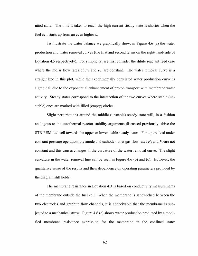
nited state. The time it takes to reach the high current steady state is shorter when the
fuel cell starts up from an even higher λ.
To illustrate the water balance we graphically show, in Figure 4.6 (a) the water
production and water removal curves (the first and second terms on the right-hand-side of
Equation 4.5 respectively). For simplicity, we first consider the dilute reactant feed case
where the molar flow rates of FA and FC are constant. The water removal curve is a
straight line in this plot, while the experimentally correlated water production curve is
sigmoidal, due to the exponential enhancement of proton transport with membrane water
activity. Steady states correspond to the intersection of the two curves where stable (un-
stable) ones are marked with filled (empty) circles.
Slight perturbations around the middle (unstable) steady state will, in a fashion
analogous to the autothermal reactor stability arguments discussed previously, drive the
STR-PEM fuel cell towards the upper or lower stable steady states. For a pure feed under
constant pressure operation, the anode and cathode outlet gas flow rates FA and FC are not
constant and this causes changes in the curvature of the water removal curve. The slight
curvature in the water removal line can be seen in Figure 4.6 (b) and (c). However, the
qualitative sense of the results and their dependence on operating parameters provided by
the diagram still holds.
The membrane resistance in Equation 4.3 is based on conductivity measurements
of the membrane outside the fuel cell. When the membrane is sandwiched between the
two electrodes and graphite flow channels, it is conceivable that the membrane is sub-
jected to a mechanical stress. Figure 4.6 (c) shows water production predicted by a modi-
fied membrane resistance expression for the membrane in the confined state:
62

Time [s]
10 10 10 10 102 3 4 5 62 3 4 5 60
50
100
150
200
250
300
350
400
0
50
100
150
200
250
300
350
400
Cur
rent
[mA
]
λ = 3.1
λ = 4.0
λ = 1.2
λ = 2.2
λ = 6.0
λ = 5.0
λ = 3.1
λ = 4.0
λ = 1.2
λ = 2.2
λ = 6.0
λ = 5.0
Figure 4.5: Predicting fuel cell startup with the simplified STR-PEM model. The STR-PEM model successfully captures the experimen-tally observed fuel cell startup behavior. For different initial mem-brane water contents as indicated by λ, the fuel cell current will ignite or extinguish.
63

Figure 4.6: Water management and steady state multiplicity in a PEM fuel cell. Water production (solid curve) and removal (dashed curve) are illustrated as functions of the membrane water activity, aw. The filled (empty) circles denote stable (unstable) steady states. (a) Dilute reactant feed with T = 298 K, RL = 1.2 Ω, FA = FC = 1.42x10⁻⁶ m3/s; (b) Pure reactant feed with T = 353 K, RL = 1.2 Ω, PT = 105Pa, nH2
in = nO2in = 5.7 x 10⁻⁶ mol/s (c) Pure reactant feed with a modi-
fied membrane resistance expression that gives rise to the occurrence of five steady states; three of which are stable. T = 353 K, RL = 1.2 Ω, PT = 105Pa, nH2
in = nO2
in = 5.7 x 10⁻⁶ mol/s.
64

2
7 0.2( ) 10 exp( 14 ) exp 2/ 2
w cM w w o
a x lR a a yw Aw
μπ
⎧ ⎫⎡ ⎤⎡ ⎤−⎪ ⎪⎛ ⎞= − − + −⎢ ⎥⎢⎨ ⎬⎜ ⎟⎝ ⎠⎢ ⎥⎢ ⎥⎪ ⎪⎣ ⎦⎣ ⎦⎩ ⎭
⎥ (10)
This expression (with μ = 76, yo = 0.01, w = 0.07, xc = 0.08) attempts to capture the ex-
perimental observation of “pinning” of the membrane resistance over certain intermediate
ranges of water activity. We believe that this pinning, which causes the membrane resis-
tance to vary in a stepwise fashion as depicted in Figure 4.7, arises from the mechanical
constraints the electrode assembly imposes on the swelling membrane. As Figure 4.6 (c)
shows, this can lead to five total (three stable) steady states, consistent with experimental
observations (Moxley et al., 2003).
The water balance diagrams in Figure 4.6 can be used to explore the dependence
of cell ignition on operating parameters. Temperature mainly affects water removal
through the water vapor pressure since higher temperatures are expected to increase the
slope of the water removal curve. The load resistance, on the other hand alters water
production such that increasing RL depresses the water production curve, especially at
high water activities. Higher reactant flow rates tilt the water removal curve higher. It is
interesting to observe that prehumidification of the reactant feeds translates the water re-
moval line/curve to the right. These considerations elucidate the way steady state multi-
plicity depends on parameters. Before a more systematic presentation of these results, a
caveat: the validity of both the data and the model predictions is limited to water activi-
ties less than (possibly approaching) one. Predictions of our simplified model beyond
this limit are invalid; they signal conditions under which condensation of liquid water
will occur (something experimentally observed). An extension to a two-phase model will
be required to quantify such operation.
65

4.3 Figure 4.7: The membrane resistance based on conductivity measurements on an unconfined Nafion 115 membrane exponentially decreases with the membrane water activity. A membrane sandwiched in between the electrodes and graphite plates is subjected to an additional mechanical stress which gives rise to the pla-teau observed in the membrane resistance. The five steady states observed in an STR-PEM fuel cell are attributed to this membrane pinning phenomena.
66
A Computational Parametric Study
We use continuation/numerical bifurcation techniques implemented in the soft-
ware AUTO to identify regions in parameter space where steady state multiplicity exists
(Doedel, 1981). The four experimentally controllable parameters, T, RL, 2
inHn , and are
varied in our computations. Since we assume that water in the membrane and water in
the vapor phase are in equilibrium, constant pressure operation at 1 bar indirectly estab-
lishes a maximum temperature of 373 K that is allowable in the fuel cell.
The continuation results are organized in terms of three two-parameter bifurcation
diagrams: T and RL in Figure 4.8; T and
2
inOn
2
inHn in Figure 4.9 (a); and
2
inOn
2
inHn in Figure 4.9
(b). Regions of one, three, and five steady states are marked I, III and V respectively.
Blowups of the first two diagrams are included as insets, to provide a better feeling of
steady state multiplicity over larger parameter ranges. Representative one-parameter cuts,
marked on the two-parameter diagrams by α and β, are included to illustrate the various
ignition-extinction transitions involved. The ordinate of the one-parameter diagrams
show the steady state cell current density which reflects water production in the fuel cell.
Ignited branches are characterized by high current densities whereas extinguished
branches are represented by lower current densities. Solid curves in the one-parameter
bifurcation diagrams denote stable steady states while dashed curves correspond to un-
stable ones.
67

Load
Res
ista
nce
[Ω]
Temperature [K]320
10
330 340 350 360 3700
1
2
3
4
5
6
7
8
9
I
Load
Res
ista
nce
[Ω]
Temperature [K]320
10
9
8I
7
6
5
4
3
2
1
0330 340 350 360 370
Figure 4.8: Two-parameter bifurcation diagram in T and RL for nH2in = nO2
in = 5.7 x 10⁻⁶ mol/s. Regions of one, three, and five steady states are marked by I, III, and V. Corresponding one-parameter continuation diagrams with respect to temperature and load resistance are shown in (α1)-(α3) and (β1)-(β3) respec-tively. The solid (dashed) curves denote stable (unstable) steady states.
68

Figure 4.8 depicts a two-parameter bifurcation diagram in the load resistance -
temperature plane with inlet gas rates of 5.7 x 10⁻⁶ mol/s (10 mL/min). Figure 4.8 (α1)-
(α3) constitute representative one-parameter diagrams with respect to temperature at load
resistance values of 15 Ω, 2.5 Ω, and 1.0 Ω respectively. For all these resistances, going
below a temperature of about 325 K will cause an ignition. At these low temperatures the
vapor pressure of water is so low that water is not convected away by the gas and builds
up in the membrane, resulting in ignition. Although five steady states (of which three are
stable) are observed for the 2.5 Ω and 1.0 Ω load resistances, only a maximum of three
steady states (with two stable) is attainable for the large load resistance of 15 Ω (α1). In
addition, the cell current density at the ignited state is significantly lower compared to
current densities obtained for smaller load resistances.
Similar one-parameter continuation diagrams in the load resistance at different
temperatures are shown in Figure 4.8 (β1)-(β3) for temperatures of 322 K, 350 K, and 356
K respectively. From the cut at β1, which intersects regions with one and three steady
states, we see that the multiplicity region at 322 K spans the largest range of load resis-
tances even though the current is lower. These one parameter cuts in temperature also
indicate that for all temperatures, the fuel cell current extinguishes above a critical load
resistance.
A two-parameter continuation of turning points in the hydrogen feed and tempera-
ture plane is shown in Figure 4.9 (a). Note that the dotted curve in Figure 4.9 has been
shifted a little to the right to increase visibility of the two smaller three steady state
69

1
2
3
4
5
6
0
Inle
t hyd
roge
n m
ol/s
]
Temperature [K]
320 330 340 350 360 370310300
x10-5
1.0
1.5
0
0.5
Inle
t hyd
roge
n [m
ol/s
]
Inlet oxygen [mol/s]1.0 1.50.50
x10-5
x10-5
nH2 nH2
1
2
3
4
5
6
0
Inle
t hyd
roge
n m
ol/s
]
Temperature [K]
320 330 340 350 360 370310300
x10-5
1.0
1.5
0
0.5
Inle
t hyd
roge
n [m
ol/s
]
Inlet oxygen [mol/s]1.0 1.50.50
x10-5
x10-5
nH2 nH2
Figure 4.9: Two-parameter bifurcation diagram (a) T and nH2
in for RL=1.2 Ω , nO2in = 5.7 x 10⁻⁶ mol/s (b) nO2
in and nH2in for
T=353 K, RL=1.2 Ω. Corresponding one-parameter continuation with respect to temperature and to hydrogen feed are shown in (α1)-(α2) and (β1)-(β2) respec-tively.
70

regions. Representative one-parameter continuation diagrams with respect to temperature
are shown at constant hydrogen feed rates of 5.7 x 10⁻⁶ mol/s (α1) and 4.0 x 10⁻⁵ mol/s
(α2). Corresponding one-parameter diagrams with respect to hydrogen feed are depicted
for fixed temperatures of 330 K (β1) and 353 K (β2).
Increasing the hydrogen feed convects the water product out faster, resulting in a
drier membrane. Therefore, a comparison of the one parameter cuts in α1 and α2 indicate
that the multiplicity region shifts towards lower temperatures when the hydrogen feed
flow rate is increased. Since the vapor pressure of water increases with higher tempera-
tures, from the one parameter cuts at β1 and β2, the final extinction is observed at lower
hydrogen flow rates. In the one-parameter continuation with respect to temperature
shown in Figure 4.9 (α1)-(α2), the most noticeable feature is the proximity of the two ig-
nition points apparent in each. Cusp points and double-limit points (suggestive of a swal-
lowtail organizing center) appear in our study (Guckenheimer and Holmes, 1983). No
codimension two bifurcations were visible in the two-parameter diagram in the inlet hy-
drogen and inlet oxygen feed rate planes in the region covered in Figure 4.9 (b).
4.4 Summary
We have demonstrated, through a simplified but physically reasonable model of
an STR-PEM, the occurrence of steady state multiplicity in PEM fuel cells. The steady
state multiplicity is caused by the autocatalytic nature of the interplay between water that
is produced in the fuel cell and the reaction rate itself, which is enhanced through mem-
brane humidification. This creates a succinct analogy with the energy balance of an
71

72
autocatalytic CSTR: water activity in the STR-PEM corresponds to temperature in the
CSTR.
Water production and removal are analogous to heat production and removal, and
the corresponding straight removal line and sigmoidal production curve remarkably per-
sist in the analogy. Inlet feed humidification in the STR-PEM is analogous to inlet feed
temperature for a CSTR while the load resistance in the STR-PEM is analogous to reac-
tion enthalpy in a CSTR. Another similarity is that the feed flow rates convect away the
reaction product in both cases. Membrane swelling against mechanical constraints adds a
five steady state “twist” to the STR-PEM dynamics, reminiscent of the richness of dy-
namics of exothermic reactions in series in a CSTR.
We have shown preliminary experimental results of sustained periodic and even
chaotic oscillations in the differential STR-PEM fuel cell. In an integral PEM fuel cell
reactor there is evidence of high-current, high local water content “wet spots,” clearly
analogous to tubular reactor “hot spots.” The CSTR model presented here can be ex-
tended and effectively employed as “tanks in series” models of complex fuel cell geome-
tries. Effective control for fuel cell vehicles will not be possible until the physical
mechanisms and time scales of these complicated dynamics are understood.

Chapter 5
The STR-PEM Fuel Cell as a Reactor Building Block In this chapter, we explore how the STR-PEM fuel cell (a differential reactor) can serve
as a building block to approximate the more common integral type PEM fuel cells that
contain more complicated flow channels. The approximation consists of connecting sev-
eral of the STR-PEM fuel cells physically in series to each other. Here, we describe the
rationale behind using the STR-PEM fuel cell as a reactor building block and present re-
sults that illustrate the existence of a water front within the fuel cell.
5.1 Tanks in Series
We have previously established that the STR-PEM fuel cell is a differential reac-
tor which contains well mixed reactants and products throughout the anode and cathode
chambers. Having a STR-PEM fuel cell simplified the experimental and modeling ef-
forts since the spatial variations in concentration within the fuel cell was effectively re-
moved. Recall that the only concentration gradient is transverse to the membrane in a
STR-PEM fuel cell and it is effectively one dimensional. Because the STR-PEM fuel
73
cell is a differential reactor, we can connect several of these fuel cells physically in series
to mimic the integral type PEM fuel cells (two dimensional PEM fuel cells) that contain
spatial variations in current along the membrane. The concept of connecting STR-PEM
fuel cells stems from the classic chemical engineering example of chemical reactors in
series; CSTRs have routinely been linked in series to mimic plug flow reactors (PFRs)
(Aris, 1965; Froment and Bischoff, 1979).
The STR-PEM fuel cells are connected such that the exiting flow streams from
one tank become the inlet streams to the subsequent tank as depicted in Figure 5.1. The
reactants can be fed into the tanks in a co-current flow scheme or they can be fed into the
first and last tank such that the anode and cathode flows are counter-current to each other.
Physically connecting the STR-PEM fuel cells in series enables us to monitor the changes
in reactant and product concentration between the feed and exit streams which result in
current variations along the membrane surface. Depending on the adopted flow pattern,
flow rates, operating temperature, and external load resistance, in addition to the fuel cell
orientation (vertical or horizontal), concentrations from tank to tank differ.
5.2 The Segmented Anode Parallel Channel Fuel Cell
Instead of physically connecting several individual STR-PEM fuel cells to model
the integral reactor, we designed the tanks in series fuel cell as one unit as shown in Fig-
ure 5.2 (a). The membrane electrode assembly (MEA) is sandwiched between two Tef-
lon blocks that contain graphite inserts. The Teflon blocks are placed between two alu-
minum blocks that were heated with stainless steel sheath cartridge heaters. A CN9000A
Omega Engineering autotune temperature controller was used to monitor and control the
74

membrane
Figure 5.1: Schematic representation of several stirred tanks in series shown here with the inlet feeds to the same tank (co-current flow). Tran-sport through the membrane is coupled from tank to tank.
75

fuel cell temperature. Reactant gases were fed from the same end into the anode and
cathode flow channels (co-current) or fed from opposite ends of the fuel cell (counter-
current). Exit flows from the fuel cell were fed into two graduated flow channels that
contained water to prevent reactant backflow into the flow channels. Omega FMA
A2400 mass flow controllers for hydrogen and oxygen were used to control reactant flow
rates into the fuel cell between 1 and 10 mL/min.
The fuel cell was constructed with graphite flow channels that are 2 mm x 2 mm x
30 mm. Three of these flow channels were machined in parallel on the graphite which
was inserted into a supporting Teflon block. The anode side, more appropriately referred
to as the segmented anode, consisted of six individual graphite pieces separated by Teflon
spacers as shown in Figure 5.2 (b). Each of these graphite segments effectively acted as
an individual stirred tank reactor. The remaining reactant gases and product flows that
exit from each segment become the inlet flow to the subsequent segment. The MEA con-
sisted of two E-TEK electrodes that were hot pressed onto a Nafion 115 membrane. The
membranes were coated with a platinum catalyst loading of 0.6 mg/cm2 before hot press-
ing at 130°C and 1000 kg force for 90 seconds.
Copper sheets were placed on the back of the graphite pieces and lead wires were
soldered onto these sheets. The wires extended from the copper sheet through the Teflon
and aluminum blocks and were each connected to a 0.2 Ω sensing resistor. All six wires
were then connected together with the common lead connected to a 10 turn 0 to 20 Ω po-
tentiomenter (external load resistance). The circuit was connected to a CYDAS
1001DAP data acquisition board with 8 differential inputs to record the current measure-
ments for each segment. We utilized separate graphite pieces for the anode because
76
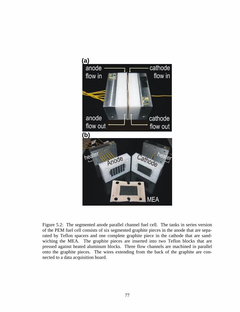
(a)
Figure 5.2: The segmented anode parallel channel fuel cell. The tanks in series version of the PEM fuel cell consists of six segmented graphite pieces in the anode that are sepa-rated by Teflon spacers and one complete graphite piece in the cathode that are sand-wiching the MEA. The graphite pieces are inserted into two Teflon blocks that are pressed against heated aluminum blocks. Three flow channels are machined in parallel onto the graphite pieces. The wires extending from the back of the graphite are con-nected to a data acquisition board.
(b)
77

we needed to keep them electrically disconnected to obtain individual current measure-
ments through each of the anode segments and voltage across the external load. The cur-
rent measurements provided an indication of the amount of water produced in each seg-
ment and the current profile downstream from the anode inlet.
Although these segments are physically connected in series, they are electrically
connected in parallel to each other as illustrated in Figure 5.3 (a) where iMR represents
the membrane resistance associated with each tank. One can visualize the tanks (seg-
ments) in series as one large resistor with an equivalent resistance calculated according to
resistances in parallel such that
1
11
eqM N
ii M
R
R=
=∑
(5.1)
The external load resistance RL can be seen to be electrically in series with the equivalent
resistance eqMR in Figure 5.3 (b). The current passing through the external load resistance
is the sum of the currents from each tank.
The segmented anode fuel cell could be positioned with the gas flow channels in a
horizontal or vertical orientation as illustrated in Figure 5.4 with reactant flows through
the fuel cell in a co-current or counter-current scheme. When the flow channels were ori-
ented vertically, both reactants were fed from the top in the co-current scheme but the
feed into the anode was fed from the bottom in the counter-current flow scheme. Feed
flow into the cathode remained from the top to bottom in both flow schemes to ease
78

Figure 5.3: Equivalent electrical circuit for the segmented anode fuel cell. (a) Each segment is associated with an internal membrane resistance which is electrically connected in parallel to other segments (b) The equivalent re-sistance for these six segments is electrically in series with the external load resistance.
Figure 5.4: The segmented anode fuel cell configuration. The flow channels can be oriented (a) horizontally or (b) vertically. The fuel cell configuration is an important consideration when there is liquid water formation.
79

transport of liquid water out of the fuel cell. Under conditions where liquid water forma-
tion occurred, we found that the gas flow channel orientation was an important considera-
tion. The segments are numbered from 1 thru 6 beginning with the segment closest to the
anode inlet.
5.3 Current Evolution
We first monitored the current evolution in the segmented anode parallel channel
fuel cell in a horizontal position (see Figure 5.5) and as expected, found measurable dif-
ferences in currents downstream from the anode inlet. The MEA was equilibrated at
room temperature conditions before it was assembled into the segmented anode fuel cell.
Upon assembling the fuel cell, hydrogen and oxygen flows were started at 5 mL/min and
fed co-current to the fuel cell with the external load resistance fixed at 3.5 Ω. For this
initial run, the fuel cell was not heated. The membrane was sufficiently hydrated at the
start so that we were able to measure a current as soon as we began operating the fuel cell.
Over the first several hours, the fuel cell equilibrated slowly to the new operating
conditions and the currents in each segment were observed to reach a slight plateau. Dur-
ing this time, the current in the second segment was largest at 41 mA while the current in
the last tank was the lowest at about 20 mA. This type of current distribution is expected
for a fuel cell operating with co-current flows because more reactant reaches the front
portion of the fuel cell (the part that is closer to the anode inlet). Since the initial mem-
brane water content is uniform throughout the entire fuel cell, the initial current produc-
tion is dependent on the amount of reactant reaching the electrodes within each segment.
80

Figure 5.5: Current profiles in each segment over time for the fuel cell equilibrated at room temperature with reactant flow rates of 5 mL/min fed in co-current configuration and an external load resistance of 3.5 Ω. The gas flow channels were oriented horizontally.
81

Despite maintaining fixed operating conditions, the currents in each segment are ob-
served to change somewhat dramatically after 10 hrs. We observed a rather sharp decline
in the current in the second and fifth segments which was accompanied by an increase in
current for the third and sixth segments. We believe that this change in current is attrib-
utable to a shift in the membrane water content downstream. With the larger initial cur-
rent in the second segment, more water was produced in this segment resulting in a wetter
portion of the membrane. Over time, the portion of the membrane in the second segment
becomes saturated with water. Eventually, the water content in the neighboring portion
of the membrane, the third segment, will also experience an increase in water content.
This autocatalytically drives the reaction further and results in the increased current pro-
duction there in the third segment. The decrease and increase in current observed for the
fifth and sixth segments respectively are attributed to a similar effect of water transport in
the portion of the membrane from the fifth to the sixth segment. The total current over
the 24 hr period increased from 166 mA to 182 mA.
5.3.1 Ignition Fronts and Propagation
We studied ignition fronts for the fuel cell in both the horizontal and vertical flow
channel configurations under both co- and counter-current reactant flows. The fuel cell
was started up from an extinguished current state and the current profiles were monitored
over time. The fuel cell was equilibrated with a hydrogen flow rate of 4 mL/min and an
oxygen flow rate of 6 mL/min.
In the first study, the fuel cell current was previously extinguished at 75°C with
reactants in counter-current flow. After extinguishing the current, the fuel cell tempera-
ture was lowered to room temperature while the load resistance was set to 20 Ω (to pre-
82

vent the cell from igniting during cooling). When the cell had reached room temperature,
the external load resistance was set to a low load of 0.25 Ω to facilitate ignition. A color
plot of the current profile downstream from the anode inlet as a function of time is pre-
sented in Figure 5.6 (a). From this plot, we observe that the fuel cell remained extin-
guished for some time and eventually started to ignite from the middle of the fuel cell.
The sudden increase in current first occurred in the third segment and propagated out-
wards to the front (anode inlet) and back (anode exit). The darker red regions in the plot
represent regions of high current and are wet spots in our fuel cell that are reminiscent of
hot spots in the classic textbook examples of plug flow reactors (Aris, 1965; Froment and
Bischoff, 1979). These wet spots are observed to move across the fuel cell over time.
After the current in segment three reaches a maximum of 100 mA, the current production
there begins to decline, while the current production increases downstream. The current
profile across the fuel cell continues to evolve as the fuel cell strives to maintain a suit-
able balance between water production and water removal.
For the co-current operation under hydrogen and oxygen flow rates of 6 mL/min
and 4 mL/min, ignition was recorded for the fuel cell equilibrated at a higher temperature
of 60°C. Under the co-current flow scheme, the fuel cell was observed to ignite nearer to
the anode exit in comparison to counter-current flow. As shown in Figure 5.6 (b) ignition
was first observed in segment 5 and the current then propagated out towards the front and
end of the fuel cell. Segment 4 ignited later than expected and the current in this segment
was lower than the currents recorded for the neighboring segments 3 and 5.
Note that in Figure 5.6 (b), the red colored region appears divided by the low cur-
rent in segment 4. The low current recorded for segment 4 is attributed to a reduced
83

(a) (b)
Figure 5.6: Ignition fronts for a horizontally oriented flow channel fuel cell with hydrogen and oxygen flow rates of 4 mL/min and 6 mL/min respectively. The colors represent the dif-ferent intensities in cell current (mA). The cell current in each segment is plotted downstream from the anode inlet as a function of time: (a) Counter-current flows at 25°C. The current in segment 3 is the earliest to ignite and the front propagates to the edges; (b) Co-current flows at 60°C. Ignition first occurred in segment 5.
(a) (b)
Figure 5.7: Ignition fronts for the vertically oriented flow channel with equal hydrogen and oxygen flow rates of 3.5 mL/min at 25°C: (a) Counter-current flow; (b) Co-current flow.
84

contact between the anode graphite insert and copper sheets. Note that the graphite and
Teflon inserts are pushed into the Teflon backing, which sandwiches the MEA with the
cathode piece. Wires were soldered onto the copper sheets so that the wire contacts the
graphite insert. Both the anode and cathode blocks are fastened on each side with 6 nuts.
If a portion of the fuel cell is slightly loose, the anode graphite insert at this loose portion
will be slightly raised from the copper sheet, reducing contact with the wire.
In addition, operating the fuel cell with the gas flow channels configured horizon-
tally was not optimal since liquid water could accumulate in the lowest flow channel, pre-
venting the transport of reactants to available reaction sites there. As a result of the unde-
sirable water build-up in the lower channels, we operated the fuel cell with the gas flow
channels oriented vertically. In this configuration, any liquid water formed in the cathode
compartment would drain downwards. In addition, the oxygen supply was fed into the
cathode from the top to aid water removal by pushing the liquid down. We also recorded
ignition effects in this configuration for both the counter-current and co-current flow
scheme. The fuel cell was first extinguished with a high external load resistance of 20 Ω
(to mimic open circuit conditions) at a high temperature of 75°C with hydrogen and oxy-
gen flow rates of 10 mL/min into the fuel cell.
To observe ignition, the fuel cell was first cooled to room temperature. After the
fuel cell was maintained at 25°C, the external load resistance was lowered back to 0.25 Ω
with hydrogen and oxygen flows of 3.5 mL/min in counter-current. Ignition in the verti-
cally oriented flow channels with counter-current gas flows occurred after an induction
period of about several hours as shown in Figure 5.7 (a). Similar to the previous example
of counter-current ignition in the horizontally oriented gas flow channels, we again ob-
85

serve that the fuel cell current first ignited in the third segment. The current then fanned
out to the front end and the back end of the cell. However, in comparison to the horizon-
tally oriented segmented anode fuel cell, the current generated in the vertical configura-
tion was significantly larger. Focusing on the third segment alone, we see that a maxi-
mum current of 200 mA is produced in comparison to the 100 mA obtained from the
horizontally oriented fuel cell.
By comparing the color plots in Figures 5.6 (a) and 5.7 (a) and considering the
different range in current intensities (as indicated by the color bar to the right of each
plot), the current generated in all the ignited segments of the vertically oriented fuel cell
is larger than that produced in the horizontally oriented fuel cell. Since we operated the
fuel cell at room temperature, it is conceivable that liquid water formed in the fuel cell.
Figure 5.7 (a) indicates that the currents in the portion of the fuel cell closer to the anode
inlet remained higher, suggesting that liquid water formed in the cell indeed accumulated
near the bottom of the cell and hindered reactant mass transfer there (as suggested by the
lower currents in the segments nearer to the anode exit). In addition, the larger current
regions remained relatively fixed around the second and third segments.
Ignition fronts for the vertically configured flow channels with co-current reactant
flows were also recorded. The fuel cell was extinguished with the same pre-treatment
described for the counter-current fuel cell in the vertical configuration. We later cooled
the fuel cell to 25°C, lowered the external load resistance to 0.25 Ω, and supplied hydro-
gen and oxygen gases at 3.5 mL/min to the anode and cathode in co-current. Both feeds
were supplied from the top of the fuel cell. Unlike ignition fronts observed for the
counter-current flow scheme, here we see that ignition first occurred in the segment far-
86

thest away from the anode inlet in segment 6 and propagated towards the inlet as shown
in Figure 5.7 (b).
The wet spots that initially appear in the back portion of the fuel cell also propa-
gate towards the front of the cell. The starkly different ignition fronts for the two differ-
ent flow schemes are not surprising. In the co-current flow, it is easier for the portion of
the membrane associated with segments that are farther away from the inlet streams to
accumulate enough water for ignition since the flow is downwards from the top. Recall
that the segments are numbered starting from the anode inlet. However, once the differ-
ent segments have ignited, current production is higher for segments that are closer to the
inlet streams. This increased current production near the inlet can be attributed to:
(i) liquid water accumulation in the gas channels of segments closer to the bot-
tom of the fuel cell hinders mass transport of the reactants to the electrodes.
(ii) more reactant reaching and consumed in the front portion of the cell
When the fuel cell has equilibrated to the operating conditions after ignition, the co-
current flow fuel cell produces a total current of 360 mA; much smaller than the total cur-
rent produced in the counter-current flow fuel cell of about 620 mA in the same vertical
configuration (see Figure 5.8). If one were to only measure the total current produced,
ignition fronts in the segmented anode fuel cell would be overlooked as well as the dif-
ferences in current downstream from the anode inlet.
5.3.2 Extinction Fronts
In addition to the ignition fronts, extinction fronts for the fuel cell were recorded
for the horizontally oriented flow channel fuel cell with counter-current flows and the
87

Figure 5.8: Total current profiles during ignition for the vertically ori-ented fuel cell with reactants fed in: (a) counter-current; (b) co-current. The total current generated for the counter-current flow fuel cell is higher than that generated in the co-current fuel cell under identical op-erating conditions.
88

the vertically oriented fuel cell with co-current flows. The extinction front in Figure 5.9
(a) was observed for the horizontally oriented fuel cell with counter-current flows of
equal hydrogen and oxygen flow rates of 5.4 mL/min. The fuel cell was previously
equilibrated at 60°C with an external load resistance of 10 Ω. Keeping the external load
and flow rates fixed, the temperature was increased to 80°C to extinguish the current. By
increasing the fuel cell temperature, we increased the water vapor pressure, resulting in
more water flow out of the fuel cell. From Figure 5.9 (a), the current extinguished first in
the segment closest to the anode inlet after 3 hours and the extinction propagated towards
the back. Segments that produced less current at the start were the first to extinguish.
The extinction front shown in Figure 5.9 (b) was observed for the fuel cell con-
figured vertically with co-current flows. The fuel cell was operated overnight at 70°C
with reactant flow rates of 10 mL/min and an external load resistance of 2 Ω. The fuel
cell currents were observed to be declining when the external load resistance was lowered
to 0.25 Ω. The color plot in Figure 5.9 (b) depicts the fuel cell current extinction shortly
after lowering the load resistance to 0.25 Ω. Despite lowering the external load resis-
tance, the current production was not sufficiently large to prevent the fuel cell from ex-
tinguishing.
5.4 Extended Operation Results
5.4.1 Polarization Curves
Polarization curves for the segmented anode fuel cell were obtained by varying
the load resistance from 0 Ω to 20 Ω over a period of about 100 seconds. Since the load
89

(a) (b)
Figure 5.9: Extinction fronts: (a) Horizontally oriented flow channel fuel cell with counter-current reactant flow rates of 5.4 mL/min at 10 Ω and 80°C; (b) Vertically oriented fuel cell with co-current reactant flow rates of 10 mL/min at 0.1 Ω and 70°C.
90

resistance was changed over this relatively short time period, the obtained polarization
curve is referred to as an instantaneous polarization curve where the membrane water
content is expected to remain unchanged. Benziger et al. have shown that plotting the
power produced by the fuel cell as a function of the load resistance is a more insightful
representation of the polarization data (Benziger et al., in press). The power in the fuel
cell can be expressed as
22
L LeqM L
VP I R RR R
⎛ ⎞= = ⎜ ⎟+⎝ ⎠
.
At the maximum power, we find that the load resistance associated with the peak power
in the power performance curve is equal to the equivalent fuel cell membrane resistance.
In this case, eqMR represents the equivalent membrane resistance for all six segments that
are electrically connected in parallel.
( )2 2
32 L
eq eqL M L M L
dP V V RdR R R R R
⎛ ⎞= −⎜ ⎟+⎝ ⎠ +
0 eqM L
L
dP R RdR
= → =
A plot of the power performance as a function of the external load resistance is provided
in Figure 5.10 (a) for the vertically configured segmented anode fuel cell previously
equilibrated at 50°C and 4 Ω external load resistance with counter-current flows of hy-
drogen and oxygen at 10 mL/min and 5 mL/min respectively. From the plot, the equiva-
lent membrane resistance is relatively small, at about 0.6 Ω. A more conventional polari-
zation plot of voltage versus current is shown in Figure 5.10 (b). The different slopes
91

Figure 5.10: (a) Overall power performance curve for the fuel cell. The load resistance at peak power is equal to the equivalent membrane resistance for all six electrically parallel segments.
Figure 5.10: (b) Polarization curves for all six segments taken after equilibration at 50°C and 4 Ω with 10 mL/min of hydro-gen and 5 mL/min of oxygen in counter-current flow. The dif-ferent slopes indicate that each segment is associated with a different membrane resistance.
92
observed for each line indicates that the membrane resistance is slightly different within
each segment.
5.4.2 Hydrogen Crossover Effect
In addition to observing ignition/extinction fronts in the segmented anode fuel cell,
the fuel cell response to changes in other operating parameters such as the flow rates,
temperature, and the external load resistance were monitored. Although it is a combina-
tion of the operating parameters that affect the membrane water content, we can general-
ize that it is optimal to operate under moderate flow rates and temperatures to prevent
membrane dehydration. We were unable to sustain the fuel cell current when the reactant
flow rates were too large because the increased reactant flow through the channels re-
sulted in a greater rate of water removal, thereby drying the membrane more rapidly. We
have also shown that increasing the fuel cell temperature can sometimes lead to the cur-
rent extinguishing.
In one experiment, the segmented anode fuel cell was equilibrated to an increase
in the load resistance after every hour and the current evolution in each segment was re-
corded as shown in Figure 5.11. Reactant flow rates of 5 mL/min to the anode and cath-
ode were fed in counter-current flow. The fuel cell was oriented horizontally with the
operating temperature set to 60°C. In general, the fuel cell current in each segment de-
creased with the higher load for the first five hours. However, negative currents were
surprisingly measured in the last two segments of the fuel cell (segments 5 and 6). Fol-
lowing the start of these negative currents, subsequent increases in the load resistance did
not result in any substantial change in the currents in each segment. When the load resis-
93

tance was changed to 20 Ω a little after 9 hours, the currents changed very slightly. Sev-
eral autonomous steps in the current were observed at 11 hrs, 14.5 hr, and 21 hours.
Puzzled by these observed negative currents, we proceeded to decrease the load
resistance in a similar stepwise fashion as shown in Figure 5.12. As we decreased the
load, the negative currents in segments 5 and 6 became less negative. When the load re-
sistance was lowered to 4 Ω, the current in segment 5 jumped up to 10 mA. The remain-
ing negative current in segment 6 became positive when the load was further decreased to
0 Ω after 6 hours. At that same point in time, a slight decline in current was observed
following the sharp increase in current for all segments. Several other autonomous
changes in current were observed over time despite fixing all other operating parameters.
We observed negative currents for several other conditions and were rather per-
plexed by this phenomenon. However, we now believe that the negative currents arise
due to hydrogen crossover from the anode to the cathode. Crossover is not a new occur-
rence and has been observed in direct methanol fuel cells with thin membranes (Heinzel
and Barragan, 1999; Ren et al., 2000a; Ren et al., 2000b). Hydrogen crossover causes a
decrease in the open circuit voltage for the PEM fuel cell. Hydrogen crossover in seg-
ments 5 and 6 of our segmented anode fuel cell brings excess hydrogen to the cathode
which is unreacted with the oxygen at the cathode. The hydrogen is then oxidized and
driven backwards across the membrane, resulting in the negative currents. Note that
crossover is undesirable because it bypasses the electrical circuit, its normal reaction path,
to produce water directly at the cathode and therefore does not produce usable power.
94

Figure 5.11: The external load resistance effect on current. For a fuel cell with counter-current reactant flow rates of 5 mL/min at 60°C, the external load resistance was manually increased af-ter each hour. We discovered the occurrence of negative cur-rents in the last two segments of the fuel cell.
95

Figure 5.12: The effect of decreasing the external load resistance on the segmented anode fuel cell. Under the same operating con-ditions (60°C, 5 mL/min reactants) in counter-current flow, the external load resistance was decreased in a stepwise fashion from 20 Ω to 0 Ω. The fuel cell current in segments five and six be-came less negative with the increasing load resistance and eventu-ally returned to positive at 4 Ω.
96
As we increased the external load resistance, the current production in each segment de-
creased, and we inadvertently promoted hydrogen crossover due to the unused hydrogen
available in the anode flow channel. Therefore, in the latter experiment where we de-
creased the external load resistance, we increased hydrogen consumption, reduced hydro-
gen crossover and returned the fuel cell to its normal state.
5.4.3 Current Oscillations
After tracking the fuel cell response to step changes in the load resistance as de-
scribed above, we resumed studying the fuel cell extinction front. For the fuel cell with
the flow channels in the horizontal orientation, the cell temperature and external load re-
sistance were increased to 75°C and 20 Ω while the hydrogen and oxygen flow rates were
5.2 mL/min and 6 mL/min respectively in co-current scheme. Instead of observing an
extinction front, negative currents in tanks 5 and 6 were recorded along with autonomous
oscillations in the fuel cell current as shown in Figure 5.13. None of the operating pa-
rameters were changed during the duration in which the oscillations were observed. The
current oscillations were rather regular with a period of about two hours.
Since the oscillations in current were observed for the horizontally oriented fuel
cell, we believe that they arise due to liquid water flowing out of the fuel cell. As men-
tioned previously, when the flow channels are horizontal, some liquid water might accu-
mulate in the lowest flow channel, creating additional mass transport limitations. During
the experiment, plugs of water were observed to periodically flow out of the effluent
tubes of the fuel cell. When the plugs of water successfully exit the cell, a rise in the fuel
cell current is observed since the mass transport resistance for the reactant is decreased.
97

Figure 5.13: Autonomous oscillations observed for the horizontally oriented parallel channel fuel cell with co-current reactant flow rates of 5.2 mL/min of hydrogen and 6.0 mL/min of oxygen. The fuel cell temperature and external load resistance were set to 75°C and 20 Ω.
98

5.5 Summary
We have introduced here a unique version of the PEM fuel cell which utilizes the
features of an STR-PEM fuel cell as an initial approximation of the more common two
dimensional serpentine type fuel cells that frequently contain concentration variations
over the membrane. By constructing and operating the segmented anode parallel channel
fuel cell, we successfully captured the current variations downstream from the anode inlet.
This was possible because the segmented graphite pieces in the anode were electrically
connected in parallel to each other. Individual measurements of the current in each seg-
ment enabled us to observe the power production from the various segments.
From the color plots of current production across the different segments over
time, we observed the existence of wet spots (corresponding to regions of large current)
in the fuel cell that are analogous to hot spots in the familiar tubular reactor. The seg-
mented anode fuel cell has also provided an exclusive view of the ignition and extinction
fronts within the fuel cell. Differences in these fronts depend on the operating conditions
(flow rates, operating temperature, external load resistance), the adopted flow pattern (co-
or counter-current), as well as the flow channel configuration (horizontally or vertically
oriented flow channels).
We have also found that pre-equilibration conditions can affect the ignition pro-
file. While we were often able to extinguish the fuel cell by increasing the temperature,
we were not always successful in getting the fuel cell to reignite by lowering the operat-
ing temperature. This is attributed to the differences in water content that arise when the
fuel cell membrane equilibrates at various operating conditions. Recall that the mem-
brane acts as a reservoir for water and for some instances the membrane water content is
99
100
insufficient for ignition to occur. The segmented anode parallel channel fuel cell is ad-
vantageous because it enables us to pinpoint which segments are first to ignite and extin-
guish.
The segmented anode parallel channel fuel cell has provided a remarkable insight
into the polymer electrode membrane fuel cell which will aid in efforts to identify opti-
mal operating parameters. Individual current measurements in each segment led to the
discovery of negative currents within the fuel cell that are believed to result from hydro-
gen crossover. If we had only measured the total current, which remained positive during
the changes in external load resistance, we would have overlooked this crossover effect
inside the fuel cell. Understanding ignition/extinction as well as how the fronts move
will enable us to improve the existing fuel cell design. Potential modifications include a
distributed feed design where the reactants are fed along different segments of the fuel
cell to optimize the utilization.

Chapter 6
Modeling the Tanks in Series Fuel Cell We have used the single stirred tank PEM fuel cell as a building block to approximate
more conventional integral (plug flow) type fuel cell reactors. By connecting several
STR-PEM fuel cells in series, the effects of the four operating parameters (temperature,
external load resistance, inlet hydrogen and oxygen flow rates) on the current evolution in
each tank can be monitored. In the previous chapter, we introduced the segmented anode
parallel channel fuel cell as an approximation to the stirred tanks in series PEM fuel cell.
Here, we develop the tanks in series (segmented anode parallel channel) model based on
a modified version of the existing single stirred tank reactor model presented in Chapter 4.
6.1 The Modified Stirred Tank Reactor PEM Model
Recall that the flow channels are modeled as stirred tank reactors to which hydro-
gen and oxygen are fed at fixed flow rates of inAF and . These inlet flow rates along
with both the external load resistance RL and the fuel cell temperature T are controllable
inCF
101

quantities which appear as operating parameters in our model.∗ While the current
through and the voltage drop across the external load resistance are directly measurable
quantities, the membrane resistance RM is not directly measurable. The membrane resis-
tance represents the resistance to proton transport and is a strong function of water but
only weakly dependent on temperature (Eikerling et al., 1997; Hsu and Gierke, 1982;
Paddison, 2001; Thampan et al., 2000; Yang, 2003; Yang et al., 2004).
In the modified STR-PEM fuel cell model proposed here, we develop a more de-
tailed view of the cathode so that we may incorporate mass transfer effects there. Spe-
cifically, we have focused on modeling four regions within the PEM fuel cell as illus-
trated in Figure 6.1. This diagram highlights the important mass transport processes oc-
curring within the anode flow channel, membrane, cathode side catalyst/gas diffusion
layer, and the cathode flow channel. The variables within each region include the hydro-
gen and water partial pressures in the anode flow channel, 2HP and A
wP
CwP
(Pa), the mem-
brane water activity aw, the moles of water in gas diffusion layer nw,gdl (mol), and the par-
tial pressures of oxygen and water in the cathode flow channel, and (Pa). 2OP
The anode catalyst/gas diffusion layer mass transport effects are lumped into the
effective mass transfer coefficient k (1.3 x 10⁻² mol/m2-s) that governs the rate of water
transport between the membrane and the anode flow channel. This rate of water transport
is determined by the gradient in water activity as expressed by
( − )Aw wkA a a (6.1)
where is the membrane water activity and wa Awa is the anode flow channel water activity.
∗ For the single fuel cell models, the temperature gradients are small. The assumption of constant tempera-ture must be relaxed for fuel cell stacks.
102

Figure 6.1: Water Transport Processes. The model consists of four regions with water being produced in the cathode catalyst layer (effectively part of the cathode GDL). The anode GDL is ignored here since in these studies the fuel cell operates under dry anode conditions.
103
The anode flow channel water activity is expressed as the ratio of the water partial pres-
sure in the anode flow channel AwP to the water vapor pressure at the fuel cell temperature
as woP
/=A Aw w wa P P o (6.2)
The model also includes an electro-osmotic drag of water from the anode flow channel
through the term F
eow
ik . The electro-osmotic mass transfer coefficient depends on the
water activity in the anode flow as
42( ) 2( / )= =eo A Aw w w wk a P P 4
o
)
(6.3)
We will refer to the cathode catalyst/gas diffusion layer as the cathode GDL. Wa-
ter produced at the cathode catalyst (effectively part of the GDL), can enter the mem-
brane or the cathode flow channel. The rate of water transport between the cathode GDL
and the membrane depends on the gradient in water activity between the GDL and the
membrane as described by
( wgdlk'A a - a (6.4)
where gdla is the GDL water activity and k' (5.6 x 10⁻² mol/m2-s) is the effective mass
transfer coefficient for water transport between the GDL and the membrane. Similarly,
water from the GDL is transported to the cathode flow channel at a rate
(6.5) ( Cwgdlk"A a - a )
where (1.6 x 10⁻² mol/m2-s) is the corresponding mass transfer coefficient. This rate
depends on the difference between GDL water activity and cathode flow channel water
k"
104

activity, . The latter can be expressed in terms of the water partial pressure in the
cathode flow channel as
Cwa
/=C Cw w wa P P o (6.6)
Transport between the four respective regions is summarized in Table 6.1 below.
6.2 Flooding Effects at the Cathode
The mass transfer coefficients that govern the rate of hydrogen transport to the
anode catalyst and oxygen transport to the cathode catalyst are kA (5.8 x 10⁻⁶ mol/m2-s-Pa)
and kC (mol/m2-s-Pa) respectively. At steady state the rate of mass transfer to the catalyst
must equal the rate of reaction occurring at the catalyst surface; the reactant partial pres-
sures at the electrode/electrolyte interface 2
catHP and (Pa) are reduced from those in
the flow channels due to mass transfer across the GDL and can be expressed as
2
catOP
2 2
catH H
A
iP = P -2 k AF
(6.7)
2 2
catO O
C
iP = P -4 k AF
(6.8)
where F represents Faraday’s constant (96,500 C/mol).
Water is produced on the cathode side; we limit our model to conditions where
there is no liquid water in the flow channels at the anode side, so that kA remains constant.
At the cathode, our model allows for liquid water to accumulate within the catalyst layer,
creating an additional mass transport resistance for O2. We modeled the decrease in the
mass transfer coefficient by assuming that the pores in the cathode GDL will be uni-
formly filled with water. The oxygen goes through the cathode GDL pores which are
105

Rate of Transport Expression
Water transport between the membrane and the anode flow channel
( )− Aw wkA a a
Electro-osmotic drag of water from the anode flow channel
4 4)eowoP2( ) 2( /= =A A
w w wk a P
Water transport between the cathode GDL and the membrane
( )wgdlk'A a - a
Water transport from the GDL to the cathode flow channel
( )Cwgdlk"A a - a
Hydrogen transport to the anode cata-lyst
( )2 2
catA eff H Hk A P - P
Oxygen transport to the cathode cata-lyst
( )2 2
catC eff O Ok A P - P
Table 6.1: Relevant transport processes in the updated STR-PEM fuel cell model. The model consists of four regions with water being produced in the cathode catalyst layer (effectively part of the cathode GDL). The anode GDL is ignored since the fuel cell operates under dry anode conditions.
106

filled sequentially with water from the electrode/electrolyte interface to the cathode GDL
flow channel interface.
Without liquid water, the mass transfer of oxygen to the catalyst kC is at the
maximum possible rate of (5.8 x 10⁻⁷ mol/m2-s-Pa). However, kC decreases signifi-
cantly at the onset of liquid water formation at the cathode GDL and approaches a mini-
mum rate of (5.8 x 10⁻¹⁰ mol/m2-s-Pa) when the GDL is completely filled with liq-
uid water at (8.3 x 10⁻⁴ mol). Here, the maximum moles of water in the gaseous
phase is expressed as where Vgdl is the GDL volume (7.5 x 10⁻⁸ m3).
Therefore, kC is expressed as a function of the moles of liquid water present in the GDL
(mol) and has values between and as depicted schematically in Figure 6.2.
maxCk
axw wn P=
minCk
maxwn
,m /Go gdlV R
minCk
T
Lwn max
Ck
max
max min
max min1
cC L
w c c
w c
kkn k k
n k
=⎛ ⎞−+ ⎜ ⎟⎝ ⎠
(6.9)
The battery voltage Vb depends on the thermodynamic potential at standard condi-
tions Vo (1.23 V), the compositions in both the anode and cathode, and the total pressure
in each flow channel PT (105 Pa). The electron transfer reactions at the anode and cath-
ode are equivalent to chemical diodes which capture the typical Butler-Volmer kinetics.
From the equivalent electrical circuit, the diode effect is captured in the second term in
the following equation (where VT =0.05 V is the diode threshold voltage while Io = 0.002
A is the diode saturation current). The effective fuel cell voltage VFC (Volt) is derived
electrically as
⎛⎜⎝ ⎠FC b T
O
iV = V -V ln 1+ ⎞⎟I (6.10)
107

where the battery voltage is expressed as
( ) ( )( )
, ,
F2 2
2cat catH anode T O cathode T
b o 2
gdl
P P P PRTV = V + ln4 a
(6.11)
6.3 Mass Balances for the Stirred Tank Reactor PEM
Previously we have shown that the membrane resistance depends strongly on the
membrane water activity (Yang, 2003). For a membrane with thickness l (1.27 x 10⁻⁴ m)
and area A (1.5 x 10⁻⁴ m2) the membrane resistance is correlated as
5 0.2M w w
lR (a )= 10 exp(-14a )A
(6.12)
Electrically, the fuel cell current (based on Ohm’s law) is expressed as
FC
M w L
Vi =R (a )+ R
(6.13)
Writing the mass balances for relevant species in each respective region, we obtain the
following set of equations. Equations (6.16) and (6.17) describe the balance of hydrogen
in the anode and oxygen in the cathode while equations (6.18) and (6.19) describe the
inventory of water in the membrane and GDL respectively.
When there is only water vapor present in the GDL, the water activity is the ratio
of the partial pressure of water in the GDL to the water vapor pressure,
gdlw wgdla = P /P o (6.14)
108

aGDL
Figure 6.2: Cathode GDL mass transfer. Oxygen mass transport to the cathode electrode decreases rapidly after the onset of liquid water forma-tion. When liquid water appears within the layer (so that agdl is 1), kC will start decreasing and eventually will approach . min
Ck
1
nw,gdl 0 ,maxG
wn
vapor liquid
kC
0
maxck
minck
nw,gdl ,maxG
wn
0
maxwn
Lwn
109

The partial pressure of water in the GDL can be related to the moles of water in the GDL
(nw,gdl) such that the activity can be expressed as
( ) ( wogdl w,gdl gdla = n RT / V P ) (6.15)
The GDL water activity is equal to 1 when there is liquid water present (see Figure 6.2).
In the following equations, is the moles of sulfonic acid groups in the membrane
(3.5 x 10⁻⁵ mol), λ is the membrane water content defined as the number of water mole-
cules per sulfonic acid group (Yang, 2003), while
3SON
AgV and C
gV are the anode and cathode
flow channel volumes (2 x 10⁻⁷ m3).
F2 2 2
inAH H Hg in
A A
dP P PV i= F - F -RT dt RT RT 2
(6.16)
F2 2 2
inCO O Og in
C C
dP P PV i= F - F - RT dt RT RT 4
(6.17)
λ ⎛ ⎞⎜⎝ ⎠
3
Aw
SO w wgdlw w
da PdN = k'A(a - a ) - kA a -da dt P ⎟
w
o
(6.18)
C
F F⎛ ⎞⎜ ⎟⎝ ⎠
w,gdl eowwgdl gdl
wo
dn Pi i= - k'A(a - a )- k"A a - +kdt 2 P w (6.19)
Our estimates of the mass transfer coefficients are determined from fitting auto-
humidified stirred tank reactor PEM fuel cell data (Moxley et al., 2003). Based on resis-
tances in series, the expressions for the fluxes of water out from the cathode (NwC) and
anode (NwA) can be written as
"( )
' ( )'
GDL C Cw w w
GDL A Aw w
k a a Nkk a a N
k k
− =
− =+ w
(6.20)
110

We assumed that liquid water is present in the cathode GDL such that the water activity
there is equal to 1. From the experimental data, k” and the lumped mass transfer coeffi-
cient for k and k’ were determined to be on order of 10-6 mol/cm2-s. This was consistent
with the data from Moxley which indicated that the water produced in the fuel cell was
equipartitioned between the anode and the cathode.
We will consider the case of constant pressure operation in each flow channel (PT
=105 Pa) with pure reactant inlet flow rates specified by inAF and . Therefore, the par-
tial pressures of water in the anode and cathode can be expressed as
inCF
2
Aw T HP = P - P (6.20)
2
Cw T OP = P - P (6.21)
The exit flow rates on both the anode and cathode sides are FA and FC (m3/s). In the an-
ode, the respective terms in the expression for FA represent the moles of hydrogen enter-
ing the fuel cell, the rate of water transferred between the membrane and the anode flow
channel, the rate of water electro-osmotically dragged away from the anode, and the rate
of water production. Similarly, FC in the cathode depends on the moles of oxygen enter-
ing the cathode flow channel, the rate of water transferred between the cathode GDL and
the cathode flow channel, in addition to the rate of oxygen consumption.
( )0
0.5F
⎡ ⎤⎛ ⎞= + − − +⎢ ⎥⎜ ⎟
⎝ ⎠⎣ ⎦
Ain eowT
A A w win w T
PP iF F kA a k RTRT P P
(6.22)
0.25F
⎡ ⎤⎛ ⎞= + −⎢ ⎜ ⎟⎢ ⎥⎝ ⎠⎣ ⎦
Cin wT
C C gdlin wo T
PP i RTF F k"A a -RT P P⎥ (6.23)
111
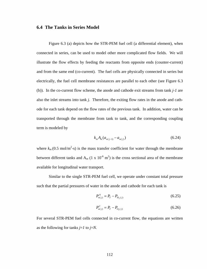
6.4 The Tanks in Series Model
Figure 6.3 (a) depicts how the STR-PEM fuel cell (a differential element), when
connected in series, can be used to model other more complicated flow fields. We will
illustrate the flow effects by feeding the reactants from opposite ends (counter-current)
and from the same end (co-current). The fuel cells are physically connected in series but
electrically, the fuel cell membrane resistances are parallel to each other (see Figure 6.3
(b)). In the co-current flow scheme, the anode and cathode exit streams from tank j-1 are
also the inlet streams into tank j. Therefore, the exiting flow rates in the anode and cath-
ode for each tank depend on the flow rates of the previous tank. In addition, water can be
transported through the membrane from tank to tank, and the corresponding coupling
term is modeled by
(6.24) ( 1) ( )(m m w j w jk A a a− − )
where km (0.5 mol/m2-s) is the mass transfer coefficient for water through the membrane
between different tanks and Am (1 x 10⁻⁶ m2) is the cross sectional area of the membrane
available for longitudinal water transport.
Similar to the single STR-PEM fuel cell, we operate under constant total pressure
such that the partial pressures of water in the anode and cathode for each tank is
(6.25) 2( ) ( )= −A
w j T H jP P P
(6.26) 2( ) ( )= −C
w j T O jP P P
For several STR-PEM fuel cells connected in co-current flow, the equations are written
as the following for tanks j=1 to j=N.
112

2 2 2( ) ( 1) ( ) ( )( 1) ( ) 2F
−−= −
AH j H j H jg
A j A j
dP P PVF F
RT dt RT RT− ji
(6.27)
2 2 2( ) ( 1) ( ) ( )( 1) ( ) 4F
−−= −O j O j O j jC
C j C j
dP P P iVF F
RT dt RT RT− (6.28)
3
( ) ( )( ) ( ) ( ) ( 1) ( ) ( ) ( 1)
( ) 0
( ) ( ) (λ− +
⎛ ⎞= − − − + − − −⎜ ⎟
⎝ ⎠
w j wA jSO gdl j w j w j m w j w j m w j w j
w j w
da PdN k'A a a kA a k A a a k A a ada dt P
) (6.29)
( ) ( ) ( ) ( )( ) ( ) ( )( )
0
( )2F F
⎛ ⎞= − − − − +⎜ ⎟
⎝ ⎠
gdl j j wC j jeogdl j w gdl j w jj
w
dn i P ik'A a a k"A a k
dt P (6.30)
( )( ) ( )( ) ( 1) ( ) ( )
0
0.5F−
⎡ ⎤⎛ ⎞= + − − +⎢ ⎥⎜ ⎟⎜ ⎟⎢ ⎥⎝ ⎠⎣ ⎦
Aw j j eoT
A j A j w j w jw T
P iP RTF F kA a kRT P P
(6.31)
( ) ( )( ) ( 1) ( )
0
0.25F−
⎡ ⎤⎛ ⎞= + − −⎢ ⎥⎜ ⎟⎜ ⎟⎢ ⎥⎝ ⎠⎣ ⎦
Cw j jT
C j C j gdl jw T
P iP RTF F k"A aRT P P
(6.32)
( ) ( )( )
2 2
2
( ) ( ) ( )( ) 2
( )
ln ln 14F
⎛= + − +⎜⎝ ⎠
cat catH j T O j T j
FC j o To
gdl j
P P P PRT iV V V Ia⎞⎟ (6.33)
( )( )
( )
−
= FC jj
M j
Vi
RV
(6.34)
( )1=
= ∑N
L jj
V R i (6.35)
6.5 Results
6.5.1 The Single Stirred Tank Reactor
The STR-PEM fuel cell will equilibrate to different steady states depending on
the operating conditions. Increasing the temperature would increase the rate of water re-
moval while increasing the load resistance would decrease the rate of water production.
113

Figure 6.3: Building blocks. (a) Several STR-PEM fuel cells can be connected in se-ries to approximate more complicated, spatially distributed, flow schemes; (b) STR-PEM fuel cell electrical circuit equivalent, with the fuel cell membrane resistances electrically connected in parallel to one another.
114

In Figure 6.4, we study a single STR-PEM fuel cell, which has initially been equilibrated
to a steady state membrane water content of aw = 0.1. The fuel cell was then set to oper-
ate at 353 K with 8.33 x 10⁻⁸ m3/s reactant feed flow rates for two different load resis-
tances: 5 Ω and 3 Ω. As shown in Figure 6.4(c), a lower steady state current is achieved
when operating the fuel cell at RL=5 Ω in comparison to RL=3 Ω. Although the 3 Ω case
yields a larger steady state current, partial flooding effects in the cathode GDL impede
oxygen transfer to the catalyst surface. The onset of liquid water formation as depicted in
Figure 6.4(a) is accompanied by a distinct drop in in Figure 6.4(b). 2
catOP
From continuation techniques in the software AUTO, we determined regions of
multiplicity in parameter space (the four controllable parameters T, RL, inAF , ). The
results are presented in three two-parameter bifurcation diagrams (T and RL in Figure 6.5
(a), T and
inCF
inAF in Figure 6.5 (b), andin
CF inAF in Figure 6.6 (a)). Regions of three steady
states are marked by III while regions with only one steady state are indicated by I. Bi-
furcation results from the current model (solid lines) are plotted in comparison to the re-
sults from the initial model (dotted line) (Chia et al., 2004). The multiplicity regions
from the current, augmented model correspond more closely to experimentally observed
regions in parameter space, suggesting an improvement from previous work.
Selected parameter cuts across the two-parameter diagrams, illustrating the igni-
tion-extinction transitions, are included in Figures 6.5 (c) and 6.6 (b). The solid curves in
the one parameter cuts represent stable steady states while the dashed curves represent
unstable steady states. For low temperatures or low inlet oxygen flow rates, the current
in the upper stable branch is observed to decrease due to the flooding in the cathode GDL.
Since the stable steady states can be determined experimentally, one could generate the
115

Figure 6.4: Flooding effects in the cathode. The transient fuel cell behavior at RL=5 Ω (dry cathode) and RL=3 Ω (wet cathode); T=353 K; FA
in=FCin=8.33 x10⁻⁸ m3/s. For
the 3 Ω case: (a) The onset of liquid water formation; (b) The presence of liquid water leads to a drop in ; (c) The current decreases due to the limited oxygen reaching the catalyst surface.
2
catOP
116

Figure 6.5: Two-parameter bifurcation diagrams for the single STR-PEM fuel cell with GDL flooding. (a) T and RL [FA
in = 1.67 x10⁻⁷ m3/s, FCin = 2.5 x10⁻⁷
m3/s]; (b) T and FAin [FC
in = 2.5 x10⁻⁷ m3/s, RL = 5 Ω]; (c) Corresponding one parameter continuation for RL = 5 Ω, marked in panel (a) [FA
in =1.67 x10⁻⁷ m3/s, FC
in = 2.5 x10⁻⁷ m3/s]. Solid (dashed) curves denote stable (unstable) steady states.
117

Figure 6.6: Two parameter bifurcation diagram for the single STR-PEM fuel cell with GDL flooding. (a) FA
in and FCin [T=353 K, RL = 5 Ω]; the region of steady state multi-
plicity lies between the curve pairs (curves of saddle-node bifurcations); (b) Represen-tative one parameter continuation in FC
in for FAin=1.67 x10⁻⁷ m3/s as marked in (a)
where solid (dashed) curves denote stable (unstable) steady states.
Figure 6.7: Flooding Regions in Parameter Space. (a) T and RL [FA
in=1.67 x10⁻⁷ m3/s] (b) FAin and FC
in [RL = 5 Ω]
(a) (b)
118

stable branches of these one parameter cuts by manually changing one of the controllable
parameters slowly. The fuel cell would then be allowed to equilibrate to the new control-
lable parameter before the current is recorded.
We have also identified regions in parameter space where flooding occurs via
continuation. In Figure 6.7, the lines represent the onset of flooding boundary and corre-
spond to conditions where the water activity in the cathode GDL, agdl is equal to 1. From
Figure 6.7 (a), we observe that we can avoid flooding by operating the fuel cell with lar-
ger inlet oxygen flow rates . From Figure 6.7 (b), we see that the flooded region de-
creases significantly when the fuel cell temperature is increased. These diagrams indicate
that both higher operating temperatures and larger flow rates facilitate water removal,
thereby reducing the flooded region. Overall, the continuation results obtained based on
the model are important in helping us determine suitable experimental operating condi-
tions for the fuel cell
inCF
6.5.2 Multiple STR-PEM fuel cells in series
In the case of several connected STR-PEM fuel cells, the flow pattern alone can
change the current profiles in the tanks. In Figure 6.8, we present data for two STR-PEM
fuel cells connected in series operating under co-current flow and counter-current flow.
The fuel cells have been pre-equilibrated to a membrane water content of aw = 0.1 before
operating at T=353 K, RL=5 Ω, inAF = =1.67 x 10⁻⁷ m3/s. Under these conditions, al-
though both flow patterns lead to the same total current (155 mA), the current profiles
differ significantly. For the co-current flow, the current in the second tank evolves to a
much larger current (124 mA) in comparison to the current in the first tank (31.2 mA)
inCF
119
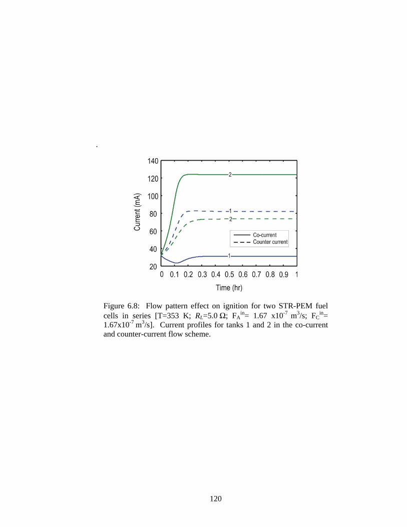
.
Figure 6.8: Flow pattern effect on ignition for two STR-PEM fuel cells in series [T=353 K; RL=5.0 Ω; FA
in= 1.67 x10⁻⁷ m3/s; FCin=
1.67x10⁻⁷ m3/s]. Current profiles for tanks 1 and 2 in the co-current and counter-current flow scheme.
120
In contrast, for counter-current flow, the currents in both tanks evolve closer together and
at steady state, the currents in the first and second tanks are 82 mA and 73.4 mA respec-
tively. These effects arise because the flow pattern affects the water content in the mem-
brane. The counter-current flow scheme sustains a higher water content in the fuel cell,
since water produced in tank 2 is brought back into tank 1 and successfully prevents the
current in tank 1 from extinguishing.
Using several STR-PEM fuel cells in series, we demonstrate that we can alter the
ignition locations and form wet spots at different locations in the fuel cell array. For a
series of six STR-PEM fuel cells in co-current flow (at T =338 K, inAF = =1.33 x 10⁻⁷
m3/s), with each tank initially pre-equilibrated at a membrane water content of aw = 0.1,
we observe the current evolution for all six tanks under two different loads, RL=6 Ω and
RL=3 Ω. As expected, a larger total current (325 mA) is observed for the smaller load of
3.0 Ω, in contrast to the total current for 6 Ω (157 mA). However, it is interesting to see
that the current profiles are very different for both load resistance values.
inCF
In Figure 6.9 (a), the steady state current is largest in the last tank and lowest in
the first. In contrast, when the tanks are operating at 3 Ω, the steady state current is
smallest in the last tank and largest in tank 2. The difference in the current profiles is the
result of different membrane water contents along the cell array. The water activities at
the cathode GDL (agdl) are equal to 1 when there is liquid water present in the GDL. At 6
Ω, all six tanks remain dry, but at 3 Ω, partial flooding occurs initially in the last tank, as
indicated by the sudden increase in nw,gdl for tank 6 in Figure 6.9 (c). The increased liq-
uid water level propagates to tank 5 and subsequently even tanks 4 and 3 flood partially.
121

Figure 6.9: Six tanks in co-current flow. Transient current profiles (T=338 FA
in=FCin=1.33 x10⁻⁷ m3/s) in each tank for: (a) RL=6 Ω, all tanks remain
dry; (b) RL=3.0 Ω, current decreases in the end tanks; (c) RL=3 Ω, liquid wa-ter formation occurs initially in the tanks at the outflow end.
K;
(a) (b) (c)
Figure 6.10: Six tanks in counter-current flow. Transient current profiles (T=338 K; FA
in=FCin= 1.33 x10⁻⁷ m3/s) in each tank for (a) RL=6 Ω: all tanks re-
main dry; (b) RL=3 Ω current decreases in the middle tanks; (c) RL=3 Ω: liquid water first forms in the tanks in the middle.
(a) (b) (c)
122

The steady state current in tanks 3, 4, 5, and 6 are much lower in comparison to the
steady state current obtainable from these tanks had they remained dry.
The current evolution also differs between the 6 Ω and 3 Ω cases in a counter-
current scheme with the same initial membrane water content in each tank (aw = 0.1). For
the fuel cell operating at 6 Ω, as shown in Figure 6.10(a), the steady state currents in all
six tanks are smaller in comparison to the currents in Figure 6.10(b). For the lower load
resistance of 3 Ω, the steady state currents in the middle of the array (tanks 3, 4 and 5) are
lower in comparison to the currents in the tanks at the array ends. In the counter-current
scheme, flooding initially occurs in the middle, beginning in tank 4. Although some
tanks are partially flooded, the level of liquid is not enough to completely flood the GDL
and inhibit all oxygen transport to the catalyst (and subsequently extinguish the current).
6.5.3 Computational Ignition Fronts
Figures 6.11(a) and (b) are current profiles for a six cell array segmented anode
parallel channel fuel cell in co-current and counter-current flow based on the model. The
model results were obtained at 328 K and 5 Ω external load, with flow rates of 8.33 x 10⁻⁸
m3/s and 1.17 x 10⁻⁷ m3/s of hydrogen and oxygen respectively. For both flow regimes,
the model successfully captures the ignition point and front propagation. Similar to the
experimentally observed ignition fronts presented in Chapter 5, the model results show
that when the gas flow is co-current, ignition occurs at the outlet of the flow channel. On
the other hand, when the gas flow is counter-current, ignition occurs in the middle of the
cell and propagates sideways.
123

Figure 6.11: The computed ignition fronts in a segmented anode PEM fuel cell for co-current and counter-current flow. In co-current flow the current ignites at the exit to the flow channels and propagates upstream to the flow channel entrance. In counter-current flow ignition occurs at the center of the flow channels.
(a) (b)
124

In co-current flow, the small amount of water produced upstream is conducted
towards the outlet where it slowly accumulates in the membrane. When the water con-
tent increases to the point where the local membrane resistance becomes comparable to
the external load resistance the current increases rapidly, hydrating the membrane and
causing ignition. The water activity in the membrane approaches unity and liquid water
begins to accumulate in the cathode GDL. The water in the membrane moves upstream
through the membrane itself, causing the ignition to propagate upstream. The current
subsequently decreases in the downstream part of the fuel cell because liquid water ac-
cumulates in the cathode GDL causing the current to decrease in the downstream ele-
ments.
When the gases flow in counter-current fashion, the water formed at the cathode
is carried towards the anode inlet in the cathode flow channel. At the same time water
formed at the cathode is transported across the membrane to the anode where it is trans-
ported towards the anode outlet by convection. Water accumulates fastest towards the
middle of the flow channels which results in ignition at the center. Changing the ratio of
the flow rates between the anode and cathode will shift the ignition point; increasing the
anode flow rate relative to the cathode flow rate shifts the ignition point towards the an-
ode outlet. After ignition, water accumulates in the cathode GDL and the membrane.
The transport of water through the membrane from high concentration at the middle of
the flow channel towards the ends results in the ignition fronts fanning out.
The model does not capture all the features of the experiment; in particular the
experiment and model deviate at longer times after ignition. Liquid water was observed
leaving the flow channels 30-40 minutes after ignition. Gravity plays a key role in how
125

the liquid water moves through the flow channels and can alter the results dramatically if
the gas flow in the flow channel is counter to the liquid flow due to gravity. The model
only considers conditions with water vapor up to where the GDL fills with liquid, but wa-
ter does not enter the flow channel. Thus the model can capture the ignition and front
propagation, but the model begins to break down at longer times when liquid water forms
in the flow channels. The model simulations were done at a higher temperature than the
experiment because at 298 K the model could not properly account for the predicted liq-
uid water.
6.6 Summary
Previously (Benziger et al., 2004; Chia et al., 2004) we had shown, through a
simplified yet physically reasonable model of the STR-PEM fuel cell, that steady state
multiplicity occurs in the cell due to the autocatalytic nature of the water transport cou-
pled to the water production. Here, we have extended the model so that it retains the
multiplicity features of the original model while accounting for key transport processes in
the fuel cell. Incorporating mass transport processes in the gas diffusion layer accounts
more realistically for current drops that are a result of an increased mass transport resis-
tance due to flooding. We have also demonstrated (through both the single and multiple
STR-PEM fuel cells in series) that the cathode GDL flooding is marked by an increased
level of liquid water which obstructs the mass transfer of oxygen to the cathode catalyst
surface. Multiple tanks in series studies are able to capture flow pattern effects on the
cell dynamics. Using arrays of several tanks in series, we were able to detect current het-
126

erogeneities along the cell array; regions of higher current correspond to wet spots in the
fuel cell array. Ignition/extinction phenomena as observed through the updated STR-
PEM fuel cell model depend on the controllable parameters (T, RL, inAF , ). Parametric
continuation computations offer insight into suitable operating parameter settings by
identifying the flooding regions in parameter space.
inCF
The water balance in the STR-PEM fuel cell is analogous to the heat balance in
the autocatalytic CSTR. By extending our differential model to the tanks in series
scheme, we are able to mimic the integral reactor; we see that the flow pattern alone is
capable of determining whether or not the fuel cell can sustain a sufficient level of water
to ensure ignition (operation at a high steady state current). We have demonstrated the
occurrence of high water content regions within the STR-PEM fuel cell (wet spots) that
are directly analogous to high temperature regions (hot spots) in the classic tubular reac-
tor. Changing the flow pattern, in addition to manipulating the controllable parameters,
can alter the spatial location of the transient ignitions as well as the ultimate steady state
current pattern in a cell array. Initial experimental observations appear to support these
theoretical predictions (Benziger et al., 2005b).
127

Chapter 7
Conclusion
We have studied the PEM fuel cell from a chemical reaction engineering perspec-
tive and have developed a differential (stirred tank reactor) version of the fuel cell
through both experimental and computational work. The simplicity of the STR-PEM fuel
cell enables us to focus on the essential physics that give rise to rich dynamical behavior
resulting from the balance between water production and water removal in the fuel cell.
This balance is remarkably analogous to the heat balance in the classical exothermic
stirred tank reactor (Aris, 1965; Perlmutter, 1972; Schmitz, 1975; Uppal et al., 1974; van
Heerden, 1953). Water production within the fuel cell improves proton transport through
the membrane and thereby autocatalytically accelerates the reaction. We have shown that
the unique balance between water production and water removal in the STR-PEM fuel
cell gives rise to multiple steady states – as indicated by the intersections of both the wa-
ter removal and water production curves.
The dynamic STR-PEM fuel cell responses to changes in operating parameters
(external load resistance, operating temperature, reactant feed flow rates) are indicative of
128

the membrane’s role as a reservoir for water. Several characteristic times are associated
with the various physical processes in the fuel cell. The characteristic times for water
absorption into the membrane and water produced to cross the membrane are on the order
of hundreds of seconds. These characteristic times are most notable because they are
contrary to the common assumption that PEM fuel cell response times are instantaneous.
The experiments affirm that the balance between water removal and water production are
disrupted when any operating parameter is altered, resulting in a different membrane wa-
ter content – extinction is possible if the membrane water activity is not sufficiently high.
Another remarkable experimental finding is the occurrence of autonomous oscillations
within a range of operating parameters. The oscillations arise due to the interplay be-
tween the polymer membrane relaxation and membrane electrode interfacial resistance.
The novel STR-PEM fuel cell design allows us to observe these oscillations since the
spatial variations are uncoupled from the temporal ones.
As an initial approximation of the conventional serpentine type PEM fuel cell, the
STR-PEM fuel cell was used as a building block in a tanks in series mode to capture cur-
rent variations between tanks (that mimic spatial variations downstream). This was im-
plemented via a segmented anode parallel flow channel fuel cell design. In addition to
the operating conditions, the reactant flow pattern (co- or counter-current) and the flow
channel orientation (horizontal or vertical) were observed to affect the current profiles
and ignition in the fuel cell. The experimental results showed that current variations
downstream from the anode inlet exist and also indicated that the ignition profiles in co-
current and counter-current flows are different. In the co-current scheme, ignition occurs
at the segment farthest away from the reactant inlet and propagates towards the front of
129
the cell. In contrast, in counter-current flow, ignition started from the middle segment
and fanned out towards the sides.
In the modeling aspect of our work, by extending the classic exothermic stirred
tank reactor to one that is based on water production and water removal in the STR-PEM
fuel cell, our mathematical model captured the experimentally observed steady state mul-
tiplicity. A positive feedback on the transport effects in the fuel cell is analogous to the
positive feedback on the reaction kinetics in the exothermic stirred tank reactor. As the
reaction proceeds, the increased water production humidifies the membrane, resulting in
greater proton conductivity which drives the reaction even further. Thus the autocata-
lyticity in the fuel cell model is captured though the strong dependence of the membrane
conductivity on the membrane water content. Regions of multiplicity were identified via
continuation in the operating parameters.
Our initial STR-PEM fuel cell model was later modified to incorporate key mass
transport processes in the cathode side catalyst/gas diffusion layer. Flooding effects were
incorporated based on the assumption that water uniformly fills the pores in the cathode
GDL. In a subsequent extension, the modified model was also employed as a building
block in the tanks in series scheme to mimic the integral type PEM fuel cell.
In comparison to existing gas diffusion layer models (Jeng et al., 2004; Lin et al., 2004;
Pasaogullari and Wang, 2004), our methodology was a simpler and more straightforward
approach which enabled us to study the PEM fuel cell dynamics.
We have demonstrated that the cathode GDL flooding is marked by the increased
level of liquid water which prevents the mass transfer of oxygen to the cathode catalyst
surface. We have also offered more insight into suitable operating parameters by identi-
130

fying the onset of flooding in parameter space. Consistent with the experimental results
from the segmented anode parallel channel fuel cell presented in Chapter 5, high water
content regions in the tanks in series scheme are observed. These high water content re-
gions (wet spots) are directly analogous to high temperature regions (hot spots) in the
classic tubular reactor. One may easily change the flow pattern to alter the ignition loca-
tions.
Once again, it is the strong exponential dependence of the proton conductivity
with membrane water content in the polymer electrolyte membrane in addition to the dy-
namics of water absorption into the membrane itself that successfully captures the igni-
tion and front propagation effects. The model reaffirms that variations in the current den-
sity along the fuel cell flow channels and the local water content in the polymer mem-
brane exist. The model predictions for the effects of reactant flow rates, cell temperature
and load resistance on ignition are qualitatively consistent with the experimental results.
The model is only semi-quantitative because the variability of the membrane-electrode-
assemblies alters the electrode/electrolyte interfacial resistance and gas transport between
the flow channels and the electrode/electrolyte interface. The model also does not ac-
count for liquid water in the flow channels.
Although the segmented anode parallel channel version of the STR-PEM fuel cell
captures the current variations downstream, there are several limitations to the present
design. During the segmented anode operation, we observed plugs of liquid water exiting
in the effluent tubes. When the flow channels were positioned horizontally, it was hard-
est for liquid water accumulated in the lowest channel to flow out of the cell, creating a
region of high oxygen mass transport resistance. This undesirable water accumulation in
131

the lowest channel is largely due to the inlet and outlet tubing being positioned on the
same level as the center flow channel. While switching the flow channel orientation to a
vertical one was a remedy, a future design with a single flow channel would be optimal.
In addition, the fuel cell should be designed with larger aluminum and graphite dimen-
sions so that it is easier to handle. The small graphite inserts in the anode were prone to
chipping and cracking. A systematic study of the operating parameter effects on ignition
and extinction profiles in addition to steady state operation should be conducted for the
newer design.
From a modeling perspective, to make the model another step closer to the ex-
perimentally operated fuel cell, the model should include the fuel cell configuration ef-
fects on the operation. A future modification of the model should incorporate gravita-
tional effects that arise when the flow channel is oriented vertically. The gravitational
term should capture the effects of water flowing out of the fuel cell in the vertical orienta-
tion.
Since the cathode GDL flooding in the current model is based on the assumption
that the GDL pores are uniformly filled with water, it would be interesting to see whether
a different pore filling mechanism would be more appropriate (Benziger et al., 2005a).
For example, the larger pores can be modeled to fill up faster than the smaller pores,
making reactant transport through the smaller pores still feasible. This would account for
the conditions where some pores are partially flooded and other pores remain dry.
Although it would be desirable to incorporate the oscillatory behavior into the
model, a more systematic experimental study of the oscillations is needed. In addition, a
better understanding of membrane swelling and relaxation is necessary before the kinet-
132

133
ics associated with these processes can be extracted. The membrane behavior should be
characterized under similar confined conditions because the actual Nafion membrane in a
fuel cell remains sandwiched between the electrodes and graphite plates. A potential
method would be to use magnetic resonance imaging of an operating fuel cell to specifi-
cally focus on the Nafion membrane.
However, the PEM fuel cell need not be limited to the Nafion membrane alone.
In fact, the STR-PEM fuel cell is versatile enough to accommodate other membrane elec-
trode assemblies. Recent work in our group with composite membranes has shown quite
promising results. Therefore, it would also be interesting to see how the current profiles
along the membrane differ in comparison to the conventional Nafion membrane. In addi-
tion, one can also study whether the autonomous oscillations are observed with compos-
ite membranes.
From both the experimental and modeling efforts for the tanks in series fuel cell,
the ignition locations differed depending on the flow scheme (co- versus counter-current).
In addition to the flow pattern effects, it would be interesting to have a systematic study
of humidification effects on the ignition location. The anode reactant feed (hydrogen)
can be humidified to various levels by passing the reactant into a heated bubbler before it
is fed into the anode.
Although we have used the STR-PEM fuel cell as a tool to observe the rich dy-
namical behavior, the fuel cell can be made applicable to conventional demands. A con-
trol loop can be implemented around the fuel cell to study how the reactant feeds should
be regulated to maintain a desired current (meet a power requirement) (Benziger et al.,
2005b).

References
"EG&G Services, Parsons, Inc," Fuel Cell Handbook (Fifth Edition), U.S Department of
Energy, Morgantown, 2000.
Acres, G. K., "Recent advances in fuel cell technology and its applications," J. of Power
Sources, 100, 60-66, 2001.
Agrawal, R., Offutt, M., and Ramage, M. P., "Hydrogen Economy - An Opportunity for
Chemical Engineers?," AIChE J, 52(6), 1582-1589, 2005.
Amphlett, J. C., Baumert, R. M., Mann, R. F., Peppley, B. A., Roberge, P. R., and
Rodrigues, A., "Parametric Modeling of the Performance of a 5-Kw Proton-
Exchange Membrane Fuel-Cell Stack," J. of Power Sources, 49(1-3), 349-356,
1994.
Amphlett, J. C., Mann, R. F., Peppley, B. A., Roberge, P. R., Rodrigues, A., and
Salvador, J. P., "Simulation of a 250 kW diesel fuel processor PEM fuel cell
system," J. Power Sources, 71(1-2), 179-184, 1998.
Aris, R., Introduction to the Analysis of Chemical Reactors, Prentice-Hall, Englewood
Cliffs, 1965.
134

Balakotaiah, V., and Luss, D., "Exact Steady-State Multiplicity Criteria for Two
Consecutive or Parallel Reactions in Lumped-Parameter Systems," Chem. Eng.
Sci, 37, 443, 1982a.
Balakotaiah, V., and Luss, D., "Structure of the Steady-state Solutions of Lumped-
Parameter Chemically Reacting Systems," Chem. Eng. Sci, 37, 1611, 1982b.
Baughman, R. H., Zakhidov, A. A., and de Heer, W. A., "Carbon nanotubes - the route
toward applications," Science, 297(5582), 787-792, 2002.
Benziger, J., Chia, E., Moxley, J. F., and Kevrekidis, I. G., "The dynamic response of
PEM fuel cells to changes in load," Chem. Eng. Sci, 60(6), 1743-1759, 2005a.
Benziger, J., Chia, E. J., and Kevrekidis, I. G., "Ignition Front Propagation in Polymer
Electrolyte Membrane Fuel Cells," (in preparation), 2005b.
Benziger, J., Nehlsen, J., Blackwell, D., Brennan, T., and Itescu, J., "Water flow in the
gas diffusion layer of PEM fuel cells," J. Membrane Science, 261(1-2), 98-106,
2005c.
Benziger, J. B., Bocarsly, A., Chia, E. J., and Kevrekidis, I. G., "A Lumped Parameter
Dynamic Model of the Water Balance in a PEM Fuel Cell," J. Power Sources,
submitted.
Benziger, J. B., Chia, E. J., Karnas, E., Moxley, J., Teuscher, C., and Kevrekidis, I. G.,
"The Stirred Tank Reactor Polymer Electrolyte Membrane Fuel Cell," AIChE J.,
50(8), 1889-1900, 2004.
Benziger, J. B., Satterfield, M. B., Hogarth, W. H. J., Nehlsen, J. P., and Kevrekidis, I.
G., "The power performance curve for engineering analysis of fuel cells," J.
Power Sources, (in press), 2005d.
135

Bernardi, D. M., "Water-Balance Calculations for Solid-Polymer-Electrolyte Fuel-Cells,"
J. Electrochem. Soc., 137(11), 3344-3350, 1990.
Bernardi, D. M., and Verbrugge, M. W., "Mathematical-Model of a Gas-Diffusion
Electrode Bonded to a Polymer Electrolyte," AIChE J, 37(8), 1151-1163, 1991.
Bernardi, D. M., and Verbrugge, M. W., "A Mathematical-Model of the Solid-Polymer-
Electrolyte Fuel-Cell," J. Electrochem. Soc., 139(9), 2477-2491, 1992.
Bevers, D., Wohr, M., Yasuda, K., and Oguro, K., "Simulation of a polymer electrolyte
fuel cell electrode," J. of App. Electrochem., 27(11), 1254-1264, 1997.
Bogdanovic, B., Brand, R. A., Marjanovic, A., Schwickardi, M., and Tolle, J., "Metal-
doped sodium aluminium hydrides as potential new hydrogen storage materials,"
J. of Alloys and Compounds, 302(1-2), 36-58, 2000.
Chambers, A., Park, C., Baker, R. T. K., and Rodriguez, N. M., "Hydrogen storage in
graphite nanofibers," J. Phys. Chem. B, 102(22), 4253-4256, 1998.
Chia, E. J., Benziger, J. B., and Kevrekidis, I. G., "Water Balance and Multiplicity in a
Polymer Electrolyte Membrane Fuel Cell," AIChE J., 50(9), 2320-2324, 2004.
Chu, D., and Jiang, R. Z., "Comparative studies of polymer electrolyte membrane fuel
cell stack and single cell," J. Power Sources, 80(1-2), 226-234, 1999.
Deluga, G. A., Salge, J. R., Schmidt, L. D., and Verykios, X. E., "Renewable Hydrogen
from Ethanol by Autothermal Reforming," Science, 303, 993-997, 2004.
Dillon, A. C., Jones, K. M., Bekkedahl, T. A., Kiang, C. H., Bethune, D. S., and Heben,
M. J., "Storage of hydrogen in single-walled carbon nanotubes," Nature,
386(6623), 377-379, 1997.
136

Doedel, E. J., "AUTO: A Program for the Automatic Bifurcation Analysis of
Autonomous Systems," Proceedings 10th Manitoba Conference on Numerical
Mathematics and Computation, Winnipeg.
Eikerling, M., and Kornyshev, A. A., "Modelling the performance of the cathode catalyst
layer of polymer electrolyte fuel cells," J. Electroanalytical Chem., 453(1-2), 89-
106, 1998.
Eikerling, M., Kornyshev, A. A., and Stimming, U., "Electrophysical Properties of
Polymer Electrolyte Membranes: A Random Network Model," J. Phys. Chem. B,
101, 10807, 1997.
Eisenberg, A., "Clustering of ions in organic polymers, a theoretical approach,"
Macromolecules, 3, 147, 1970.
Farr, W. W., and Aris, R., "Yet Who Would Have Thought The Old Man to Have Had so
Much Blood in Him: Reflections on the Multiplicity of Steady-States of the
Stirred Tank Reactor," Chem. Eng. Sci, 41, 1385, 1986.
Froment, G. F., and Bischoff, K. B., Chemical reactor analysis and design, Wiley, New
York, 1979.
Fuller, T. F., and Newman, J., "Water and Thermal Management in Solid-Polymer-
Electrolyte Fuel-Cells," J. Electrochem. Soc., 140(5), 1218-1225, 1993.
Gierke, T. D., Munn, G. E., and Wilson, F. C., "The Morphology in Nafion
Perfluorinated Membrane Products, as Determined by Wide-Angle and Small-
Angle X-Ray Studies," J. Polymer Sci., 19(11), 1687, 1981.
137

Gottesfeld, S., and Pafford, J., "A New Approach to the Problem of Carbon-Monoxide
Poisoning in Fuel-Cells Operating at Low-Temperatures," J. Electrochem. Soc.,
135(10), 2651-2652, 1988.
Grant, P. M., "Hydrogen lifts off -- with a heavy load," Nature, 424, 129-130, 2003.
Gregory, D. P., "The Hydrogen Economy," Scientific American, 228(1), 13-21, 1973.
Grubb, W. T., and Niedrach, L. W., "Batteries with solid ion-exchange membrane
electrolytes. 2. Low-temperature hydrogen-oxygen fuel cells," J. Electrochem.
Soc., 107, 131, 1960.
Guckenheimer, J., and Holmes, P., Nonlinear Oscillations, Dynamical Systems, and
Bifurcations of Vector Fields, Springer, Harrisonburg, 1983.
Gurau, V., Barbir, F., and Liu, H. T., "An analytical solution of a half-cell model for
PEM fuel cells," Journal of the Electrochemical Society, 147(7), 2468-2477,
2000.
Gurau, V., Liu, H. T., and Kakac, S., "Two-dimensional model for proton exchange
membrane fuel cells," AIChE J., 44(11), 2410-2422, 1998.
Hamelin, J., Agbossou, K., Laperriere, A., Laurencelle, F., and Bose, T. K., "Dynamic
behavior of a PEM fuel cell stack for stationary applications," International
Journal of Hydrogen Energy, 26(6), 625-629, 2001.
Heinzel, A., and Barragan, V. M., "A review of the state-of-the-art of the methanols
crossover in direct methanol fuel cells," J. Power Sources, 84(1), 70-74, 1999.
Hsing, I. M., and Futerko, P., "Two-dimensional simulation of water transport in polymer
electrolyte fuel cells," Chem. Eng. Sci, 55(19), 4209-4218, 2000.
138

Hsu, W. Y., and Gierke, T. D., "Ion Clustering and Transport in Nafion Perfluorinated
Membranes," J. Electrochem. Soc., 129, C121, 1982.
Janssen, G. J., "A Phenomenological Model of Water Transport in a Proton Exchange
Membrane Fuel Cell," J. Electrochem. Soc., 148, A1313, 2001.
Jeng, K. T., Lee, S. F., Tsai, G. F., and Wang, C. H., "Oxygen mass transfer in PEM fuel
cell gas diffusion layers," J. of Power Sources, 138, 41-50, 2004.
Kreuer, K. D., "On the development of proton conducting polymer membranes for
hydrogen and methanol fuel cells," J. Membrane Science, 185(1), 29-39, 2001.
Lee, J. H., and Lalk, T. R., "Modeling fuel cell stack systems," J. Power Sources, 73(2),
229-241, 1998.
Lin, G., He, W., and Nguyen, T. V., "Modeling Liquid Water Effects in the Gas
Diffusion and Catalyst Layers of the Cathode of a PEM Fuel Cell," J.
Electrochem. Soc., 151(12), A1999-A2006, 2004.
Liu, C., Fan, Y. Y., Liu, M., Cong, H. T., Cheng, H. M., and Dresselhaus, M. S.,
"Hydrogen storage in single-walled carbon nanotubes at room temperature,"
Science, 286(5442), 1127-1129, 1999.
Liu, F. Q., Yi, B. L., Xing, D. M., Yu, J. R., and Zhang, H. M., "Nafion/PTFE composite
membranes for fuel cell applications," J. Membrane Science, 212(1-2), 213-223,
2003.
Mann, R. F., Amphlett, J. C., Hooper, M. A. I., Jensen, H. M., Peppley, B. A., and
Roberge, P. R., "Development and application of a generalised steady-state
electrochemical model for a PEM fuel cell," J. Power Sources, 86(1-2), 173-180,
2000.
139
Moxley, J. M., Tulyani, S., and Benziger, J. B., "Steady-state multiplicity in the
autohumidification polymer electrolyte membrane fuel cell," Chem. Eng. Sci, 58,
4705, 2003.
Nakajima, H., and Honma, I., "Proton-conducting hybrid solid electrolytes for
intermediate temperature fuel cells," Solid State Ionics, 148(3-4), 607-610, 2002.
Nguyen, T. V., and White, R. E., "A Water and Heat Management Model for Proton-
Exchange-Membrane Fuel-Cells," J. Electrochem. Soc., 140(8), 2178-2186, 1993.
Okada, T., Xie, G., and Meeg, M., "Simulation for water management in membranes for
polymer electrolyte fuel cells," Electrochimica Acta, 43(14-15), 2141-2155, 1998.
Paddison, S. J., "The modeling of molecular structure and ion transport in sulfonic acid
based ionomer membranes," J. New. Mat. Electrochem. Systems, 4, 197, 2001.
Pasaogullari, U., and Wang, C. Y., "Liquid Water Transport in Gas Diffusion Layer of
Polymer Electrolyte Fuel Cells," J. Electrochem. Soc., 151(3), A399-A406, 2004.
Perlmutter, D. D., Stability of Chemical Reactors, Prentice-Hall, Englewood Cliffs, 1972.
Perry, M. L., and Fuller, T. F., "A Historical Perspective of Fuel Cell Technology in the
20th Century," J. Electrochem. Soc., 149(7), S59-S67, 2002.
Pisani, L., Murgia, G., Valentini, M., and D'Aguanno, B., "A Working Model of Polymer
Electrolyte Fuel Cells," J. Electrochem. Soc., 149(7), A898-A904, 2002.
Raistrick, I. D., "Modified Gas-Diffusion Electrodes for Proton-Exchange Membrane
Fuel-Cells," J. Electrochem. Soc., 133(3), C123-C123, 1986.
Ralph, T. R., Hards, G. A., Keating, J. E., Campbell, S. A., Wilkinson, D. P., Davis, M.,
StPierre, J., and Johnson, M. C., "Low cost electrodes for proton exchange
140

membrane fuel cells - Performance in single cells and Ballard stacks," J.
Electrochem. Soc., 144(11), 3845-3857, 1997.
Ren, X., Springer, T. E., and Gottesfeld, S., "Water and methanol uptake in Nafion
membranes and membrane effects on direct methanold cell performance," J.
Electrochem. Soc., 147(1), 92-98, 2000a.
Ren, X. M., Zelenay, P., Thomas, S., Davey, J., and Gottesfeld, S., "Recent advances in
direct methanol fuel cells at Los Alamos National Laboratory," J. Power Sources,
86(1-2), 111-116, 2000b.
Rikukawa, M., and Sanui, K., "Proton-conducting polymer electrolyte membranes based
on hydrocarbon polymers," Progress in Polymer Science, 25(10), 1463-1502,
2000.
Rosi, N. L., Eckert, J., Eddaoudi, M., Vodak, D. T., Kim, J., O'Keeffe, M., and Yaghi, O.
M., "Hydrogen storage in microporous metal-organic frameworks," Science,
300(5622), 1127-1129, 2003.
Schlapbach, L., and Zuttel, A., "Hydrogen-storage materials for mobile applications,"
Nature, 414, 353-358, 2001.
Schmitz, R. A., "Multiplicity, Stability, and Sensitivity of States in Chemically Reacting
Systems - A Review," Chem. Eng. Rev., 148, 156, 1975.
Springer, T. E., Rockward, T., Zawodzinski, T. A., and Gottesfeld, S., "Model for
polymer electrolyte fuel cell operation on reformate feed - Effects of CO, H-2
dilution, and high fuel utilization," J. Electrochem. Soc., 148(1), A11-A23, 2001.
141

Springer, T. E., Wilson, M. S., and Gottesfeld, S., "Modeling and Experimental
Diagnostics in Polymer Electrolyte Fuel-Cells," J. Electrochem. Soc., 140(12),
3513-3526, 1993.
Springer, T. E., Zawodzinski, T. A., and Gottesfeld, G., "Polymer electrolyte fuel-cell
model," J. Electrochem. Soc., 138, 2334, 1991.
Srinivasan, S., Dave, B. B., Murugesamoorthi, K. A., Parthasarathy, A., and Appleby, A.
J., "Overview of Fuel Cell Technology," Fuel Cell Systems, L. J. M. J. Blomen
and M. N. Mugerwa, eds., Plenum Press, New York, 1993.
Standaert, F., Hemmes, K., and Woudstra, N., "Analytical fuel cell modeling," J. Power
Sources, 63(2), 221-234, 1996.
Thampan, T., Malhotra, S., Tang, H., and Datta, R., "Modeling of conductive transport in
proton-exchange membranes for fuel cells," J. Electrochem. Soc., 147, 3242,
2000.
Thirumalai, D., and White, R. E., "Mathematical modeling of proton-exchange-
membrane fuel-cell stacks," J. Electrochem. Soc., 144(5), 1717-1723, 1997.
Uchida, M., Aoyama, Y., Eda, N., and Ohta, A., "Investigation of the microstructure in
the catalyst layer and effects of both perfluorosulfonate ionomer and PTFE-
Loaded carbon on the catalyst layer of polymer electrolyte fuel cells," J.
Electrochem. Soc., 142(12), 4143-4149, 1995.
Uppal, A., Ray, W. H., and Poore, A. B., "Dynamic Behavior of Continuous Stirred Tank
Reactors," Chem. Eng. Sci, 29, 967, 1974.
van Heerden, C., "Authothermic Processes: Properties and Reactor Design," Ind. Eng.
Chem, 45, 1243, 1953.
142

Washington, G. B., "Hydrogen cars fuel debate on basic research," Nature, 422, 104,
2003.
Watkins, D. S., "Research, Development, and Demonstration of Solid Polymer Fuel Cell
Systems," Fuel Cell Systems, L. J. M. J. Blomen and M. N. Mugerwa, eds.,
Plenum Press, New York, 1993.
Wilson, M. S., Derouin, C. R., Valerio, J. A., and Gottesfeld, S., "Electrocatalysis Issues
in Polymer Electrolyte Fuel Cells," Intersociety Energy Conversion Engineering
Conference, Atlanta, GA, 1203-1208.
Wilson, M. S., and Gottesfeld, S., "High-Performance Catalyzed Membranes of Ultra-
Low Pt Loadings for Polymer Electrolyte Fuel-Cells," J. Electrochem. Soc.,
139(2), L28-L30, 1992.
Wolf, J., "Liquid hydrogen technology for vehicles," MRS bulletin, 684-687, 2002.
Yang, C. R., "Performance of Nafion/Zirconium Phosphate Composite Membranes in
PEM Fuel Cells," Princeton University, Princeton 2003.
Yang, C. R., Srinivasan, S., Bocarsly, A. B., Tulyani, S., and Benziger, J. B., "A
Comparison of Physical Properties and Fuel Cell Performance of Nafion and
Zirconium Phosphate/Nafion Composite Membranes," J. Membrane Science, 237,
145-161, 2004.
Yeager, H. L., and Steck, A., "Cation and Water Diffusion in Nafion Ion-Exchange
Membranes -- Influence of Polymer Structure," J. Electrochem. Soc., 128(9),
1880-1884, 1981.
Zaluski, L., Zaluska, A., and StromOlsen, J. O., "Nanocrystalline metal hydrides," J.
Alloys and Compounds, 253, 70-79, 1997.
143

144
Zawodzinski, T. A., Derouin, C., Radzinski, S., Sherman, R. J., Smith, V. T., Springer, T.
E., and Gottesfeld, S., "Water-Uptake by and Transport through Nafion(R) 117
Membranes," J. Electrochem. Soc., 140(4), 1041-1047, 1993.
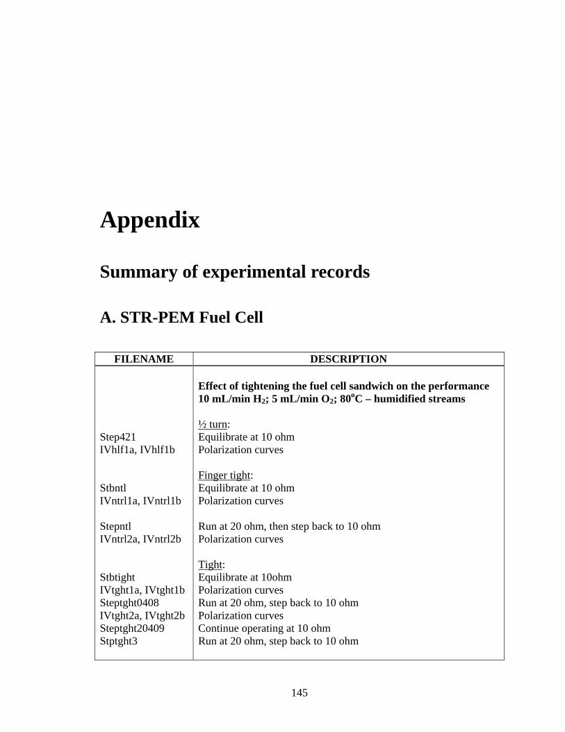
Appendix
Summary of experimental records A. STR-PEM Fuel Cell
FILENAME DESCRIPTION Step421 IVhlf1a, IVhlf1b Stbntl IVntrl1a, IVntrl1b Stepntl IVntrl2a, IVntrl2b Stbtight IVtght1a, IVtght1b Steptght0408 IVtght2a, IVtght2b Steptght20409 Stptght3
Effect of tightening the fuel cell sandwich on the performance 10 mL/min H2; 5 mL/min O2; 80oC – humidified streams ½ turn: Equilibrate at 10 ohm Polarization curves Finger tight: Equilibrate at 10 ohm Polarization curves Run at 20 ohm, then step back to 10 ohm Polarization curves Tight: Equilibrate at 10ohm Polarization curves Run at 20 ohm, step back to 10 ohm Polarization curves Continue operating at 10 ohm Run at 20 ohm, step back to 10 ohm
145

Stb0501 IV0502a, IV0502b Step0502 IV0503a, IV0503b Stb0503 IV0503a, IV0504b Step0504 IV0505a, IV0505b Stb0505, stb0506 Stb0507 IV0508a, IV0508b Stb0508 IV0509a, IV0509b Stb0509 IV0512a, IV0512b Stb0512 IV0513a, IV0513b Stb0513 IV0514a, IV0514b Stb0514 IV0515a, IV0515b Stb0515 IV0516a, IV0516b Stb0516 IV0517a, IV0517b Stb0517 IV0519a, IV0519b IV0519c, IV0519d Stb0519c IV0520a, IV0520b IV0520c, IV0520d
Effect of tightening the fuel cell sandwich on the performance 10 mL/min H2; 5 mL/min O2; 80oC – dry streams Finger tight: Equilibrate at 10 ohm Polarization curves Run at 20 ohm, step back to 10 ohm Polarization curves ½ turn: Equilibrate at 10 ohm Polarization curves Run at 20 ohm, step back to 10 ohm Polarization curves Run at 10 ohm Tight: Equilibrate at 10ohm Polarization curves Run at 10 ohm overnight Polarization curves Resume operation at 10 ohm Polarization curves Tightest: Stabilize at 4.9 ohms overnight Polarization curves Run at 5 ohms overnight Polarization curves Stabilize at 2 ohms overnight Polarization curves Resume operation at 2 ohms overnight Polarization curves Stabilize at 1 ohm overnight Polarization curves Resume operation at 1 ohm overnight Polarization curves: obtained at large current Polarization curves: obtained at low current Stabilize at 0.7 ohm Polarization curves: obtained at low current Polarization curves: obtained at large current
146

Stb0520 IV0521c, IV0521d IV0521a, IV0521b Stb0521 IV0522a, IV0522b IV0522c, IV0522d Stb0522 IV0523a, IV0523b IV0523c, IV0523d Stb0523b IV0523e, IV0523f Stb0523c IV0524a, IV0524b Stb0524b IV0525a, IV0525b Stb0525 IV0526a, IV0526b Stb0526 IV0527a, IV0527b Stb0527 IV0528a, IV0528b IV0528c, IV0528d Stb0530 IV0531a, IV0531b Stb0531 IV0601a, IV0601b Stb0528 IV0529a, IV0529b Stb0529 IV0530a, IV0530b Stb0601 IV0602a, IV0602b Stb0602 IV0604a, IV0604b Stb0604 IV0605a, IV0605b IV0605c, IV0605d
½ Tight: Load Resistance Effect Equilibrate overnight at 0.9 ohm, 80 deg C: 90 mA amplitude, 1 hr period Polarization curves: obtained at large current Polarization curves: obtained at low current Equilibrate overnight at 2 ohm, 80 deg C: 70 mA amplitude, 1 hr period Polarization curves: obtained at low current Polarization curves: obtained at large current Equilibrate overnight at 5 ohm, 80 deg C: 20 mA amplitude, 1 hr period Polarization curves: obtained at low current Polarization curves: obtained at large current Temperature Effect at RL =5 ohm Run at 5 ohm, 90 deg C (no oscillation) Polarization curves Run at 5 ohm, 70 deg C: 25 mA amplitude, 90 min period Polarization curves Run at 5 ohm, 90 deg C (no oscillation) Polarization curves Run at 5 ohm, 85 deg C (no oscillation) Polarization curves Run at 5 ohm, 60 deg C: 20 to 30 mA amplitude, 2 hr period Polarization curves Temperature Effect at RL = 2 ohm Run at 2 ohm, 70 deg C: 80 mA amplitude, 68 min period Polarization curves: obtained at large current Polarization curves: obtained at low current Run at 2 ohm, 60 deg C: oscillations died Polarization curves, after oscillations subsided Run at 2 ohm, 90 deg C: no oscillations Polarization curves Run at 5 ohm, 50 deg C: oscillations in the beginning but they fade Polarization curves Run at 10 ohm, 80 deg C: 3 mA amplitude, 42 min period Polarization curves Oxygen flow rate Effect at RL = 5 ohm, T= 80 deg C 7 mL/min H2, 3.5 mL/min O2: no oscillations Polarization curves 10 mL/min H2, 7.5 mL/min O2: no oscillations Polarization curves 10 mL/min H2, 3.0 mL/min O2: 15 mA amplitude, 48 min period Polarization curves: obtained at low current Polarization curves: obtained at high current
147

Stb0605 IV0606a, IV0606b IV0606c, IV0606d Stb0606 IV0607a, IV0607b Stb0607 IV0608a, IV0608b Stb0608 Stb0609 IV06100, IV06101 IV06110, IV06111
10 mL/min H2, 1.0 mL/min O2: 14 mA amplitude, 1 hr period Polarization curves: obtained at low current Polarization curves: obtained at high current Hydrogen flow rate Effect at RL = 5 ohm, T= 80 deg C 5 mL/min H2, 5 mL/min O2: no oscillations Polarization curves 5 mL/min H2, 2.5 mL/min O2: no oscillations Polarization curves 5 mL/min H2, 7.5 mL/min O2: no oscillations Reset load to 5 ohm Polarization curves 5 mL/min H2, 1.0 mL/min O2: no oscillations
Stb0801 Stb0804 Stb0806 Stb0807 Stb0808 Stb0809
Relative humidity sensors affixed in exit streams Run at 5 ohms, 90 deg C, 10 mL/min H2, 10 mL/min O2: - 8 mA amplitude - Fuel cell tightened to the max tightness - t > 12000s, increase RL to 20 ohm (attempt to extinguish oscillations but they persist with an amplitude of ~ 3 mA) Run at 20 ohms, 70 deg C, 10 mL/min H2, 10 mL/min O2 Run at 20 ohms, 90 deg C, 10 mL/min H2, 5 mL/min O2 (oscillations persist) Run at 10 ohms, 90 deg C, 10 mL/min H2, 5 mL/min O2 (loosened the fuel cell)
Stb0929 Stb0930a IV1003a, IV1003b Stb1003 Stb1005 Stb1006 IV1007a, IV1007b Tmp1008 IV1008a, IV1008b
Run at 10 ohms, 65 deg C, 10 mL/min H2, 5 mL/min O2 (water condensed in exiting cathode tube) Run at 10 ohms, 70 deg C, 5.5 mL/min H2, 10.2 mL/min O2 Polarization curves: RM too large, possible membrane degradation Run at 5 ohms, 70 deg C Run at 20 ohms, 70 deg C: prolonged operation at 20 ohms dehydrated the membrane Run at 2 ohms, 70 deg C, 8.2 mL/min H2, 10 mL/min O2 Polarization curves: low current Resume operation at previous conditions Polarization curves: high current
Stb1010 Stb1019 Impedancedata2.xls
Reversed anode/cathode feeds Run at 2 ohms, 70 deg C, 10 mL/min H2, 10 mL/min O2 Run at 10 ohms, 70 deg C, 5 mL/min H2, 10 mL/min O2 (no oscillations) Impedance data
148
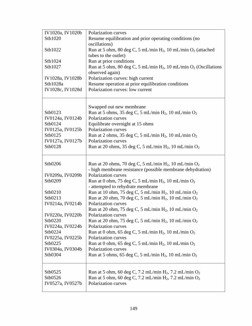
IV1020a, IV1020b Stb1020 Stb1022 Stb1024 Stb1027 IV1028a, IV1028b Stb1028a IV1028c, IV1028d
Polarization curves Resume equilibration and prior operating conditions (no oscillations) Run at 5 ohm, 80 deg C, 5 mL/min H2, 10 mL/min O2 (attached tubes to the outlet) Run at prior conditions Run at 5 ohm, 80 deg C, 5 mL/min H2, 10 mL/min O2 (Oscillations observed again) Polarization curves: high current Resume operation at prior equilibration conditions Polarization curves: low current
Stb0123 IV0124a, IV0124b Stb0124 IV0125a, IV0125b Stb0125 IV0127a, IV0127b Stb0128
Swapped out new membrane Run at 5 ohms, 35 deg C, 5 mL/min H2, 10 mL/min O2 Polarization curves Equilibrate overnight at 15 ohms Polarization curves Run at 2 ohms, 35 deg C, 5 mL/min H2, 10 mL/min O2 Polarization curves Run at 20 ohms, 35 deg C, 5 mL/min H2, 10 mL/min O2
Stb0206 IV0209a, IV0209b Stb0209 Stb0210 Stb0213 IV0214a, IV0214b IV0220a, IV0220b Stb0220 IV0224a, IV0224b Stb0224 IV0225a, IV0225b Stb0225 IV0304a, IV0304b Stb0304
Run at 20 ohms, 70 deg C, 5 mL/min H2, 10 mL/min O2 - high membrane resistance (possible membrane dehydration) Polarization curves Run at 0 ohm, 75 deg C, 5 mL/min H2, 10 mL/min O2 - attempted to rehydrate membrane Run at 10 ohm, 75 deg C, 5 mL/min H2, 10 mL/min O2 Run at 20 ohm, 70 deg C, 5 mL/min H2, 10 mL/min O2 Polarization curves Run at 20 ohm, 75 deg C, 5 mL/min H2, 10 mL/min O2 Polarization curves Run at 20 ohm, 75 deg C, 5 mL/min H2, 10 mL/min O2 Polarization curves Run at 0 ohm, 65 deg C, 5 mL/min H2, 10 mL/min O2 Polarization curves Run at 0 ohm, 65 deg C, 5 mL/min H2, 10 mL/min O2 Polarization curves Run at 5 ohms, 65 deg C, 5 mL/min H2, 10 mL/min O2
Stb0525 Stb0526 IV0527a, IV0527b
Run at 5 ohm, 60 deg C, 7.2 mL/min H2, 7.2 mL/min O2 Run at 5 ohm, 60 deg C, 7.2 mL/min H2, 7.2 mL/min O2 Polarization curves
149

B. Segmented Anode Fuel Cell
FILENAME DESCRIPTION 030905stdst 030905iva, b 031005stdst 031005iva, b 031105stdstA 031105stdstB 031105iva, b
Co-current, horizontal configuration: 3.5 ohms, Troom, 5 mL/min H2, 5 mL/min O2 Polarization curves Co-current, vertical configuration: 3.5 ohms, Troom, 5 mL/min H2, 5 mL/min O2 Polarization curves Troom, 5 mL/min H2, 5 mL/min O2 Run at 4ohm for 2 hr 40 min, increase load to 5.6 ohm Run at 2 ohm overnight Load changed to 6.24 ohms after 11 hr 45 min Load changed to 2.5 ohms after 15 hr 6 min Polarization curves
031205stdst 031205iva, b 031305stdst 031305iva, b 031405stdst 031405iva, b 031505iva, b 031605stdst 031605iva, b 031705stdst 031805stdst 032105iva, b 032205stdst 032205iva, b 032205bstdst
Counter-current, horizontal configuration: 3.5 ohm, Troom, 5 mL/min H2, 5 mL/min O2 Polarization curves 8 ohm, Troom, 10 mL/min H2, 5 mL/min O2 Polarization curves Counter-current, vertical configuration: 4 ohm, Troom, 5 mL/min H2, 5 mL/min O2 Polarization curves Counter-current, horizontal configuration Polarization curve recorded after heating at various temperatures 20 ohm, 10 mL/min H2, 10 mL/min O2 Polarization curves Co-current, vertical configuration: 20 ohm, Troom, 10 mL/min H2, 10 mL/min O2 (dry) 4 ohm, Troom, 10 mL/min H2, 10 mL/min O2 (rehydrate) Polarization curves 10 ohm, Troom, 10 mL/min H2, 10 mL/min O2 Polarization curves Counter-current, vertical configuration, H2 feed from segment 6: 10 ohm, Troom, 5 mL/min H2, 5 mL/min O2 Heat with lower watt cartridge heaters, change to horizontal configuration. Tune temperature controller.
150

032205cstdst 032205ivabriefT80 032305stdst 032305iva, b 032405stdst
Counter-current, horizontal configuration 10 ohm, 80 deg C, 10 mL/min H2, 5 mL/min O2 IV curve taken during initial cooling Resume operation at 4ohm Polarization curve 4 ohm, 65 deg C, 10 mL/min H2, 5 mL/min O2
032505stdst 032505iva, b 032605stdst 032705
Counter-current, horizontal configuration Response to heating from 65-75 deg C 4 ohm, 10 mL/min H2, 5 mL/min O2 Polarization curve 4 ohm, 75 deg C, 2.2 mL/min H2, 1.4 mL/min O2 4 ohm, 75 deg C, 3.7 mL/min H2, 6 mL/min O2 Current drops after 7 hours
032905steady11 033005steady12 033005steady13 033105steady15 040105stdst 040205stdst 040205stdstAignite 040305stdstB 040305iva, b 040305stdstRL 040405stdstdecRL
Counter-current, horizontal configuration Load was changed to 0 ohm to rehydrate the cell: ignition 0 ohm, 25 deg C, 3.7 mL/min H2, 6 mL/min O2 Load stepped from 0 – 3 ohm after 5 hrs 75 deg C, 3.7 mL/min H2, 6 mL/min O2 Dry the fuel cell 20 ohm, 75 deg C, 3.7 mL/min H2, 6 mL/min O2 Attempt to reignite after 4 hrs at 3ohm Lower temp to 50 deg C, ignition occurred At 4 hrs, increase temp to 75 deg C to dry out at 20 ohm 20 ohm, 85 deg C, 4 mL/min H2, 4 mL/min O2 0 ohm, 85 deg C, 4 mL/min H2, 4 mL/min O2 At 3 hr 30 min, flow rates changed to 5 mL/min Load increased to 4 ohm at 6 hrs, 8 ohm at 8.5 hrs 2 ohm, 85 deg C, 5 mL/min H2, 5 mL/min O2 After 2 hrs: 75 deg C After 5 hrs: 60 deg C, 4 ohm 60 deg C, 4 ohm, 5 mL/min H2, 5 mL/min O2 Polarization curve 60 deg C, 4 ohm, 5 mL/min H2, 5 mL/min O2 Resume operation at equilibrated conditions. Extinguish fuel cell by increasing the load resistance. Segments 5 and 6 extinguished. Reignite by decreasing the load resistance
151
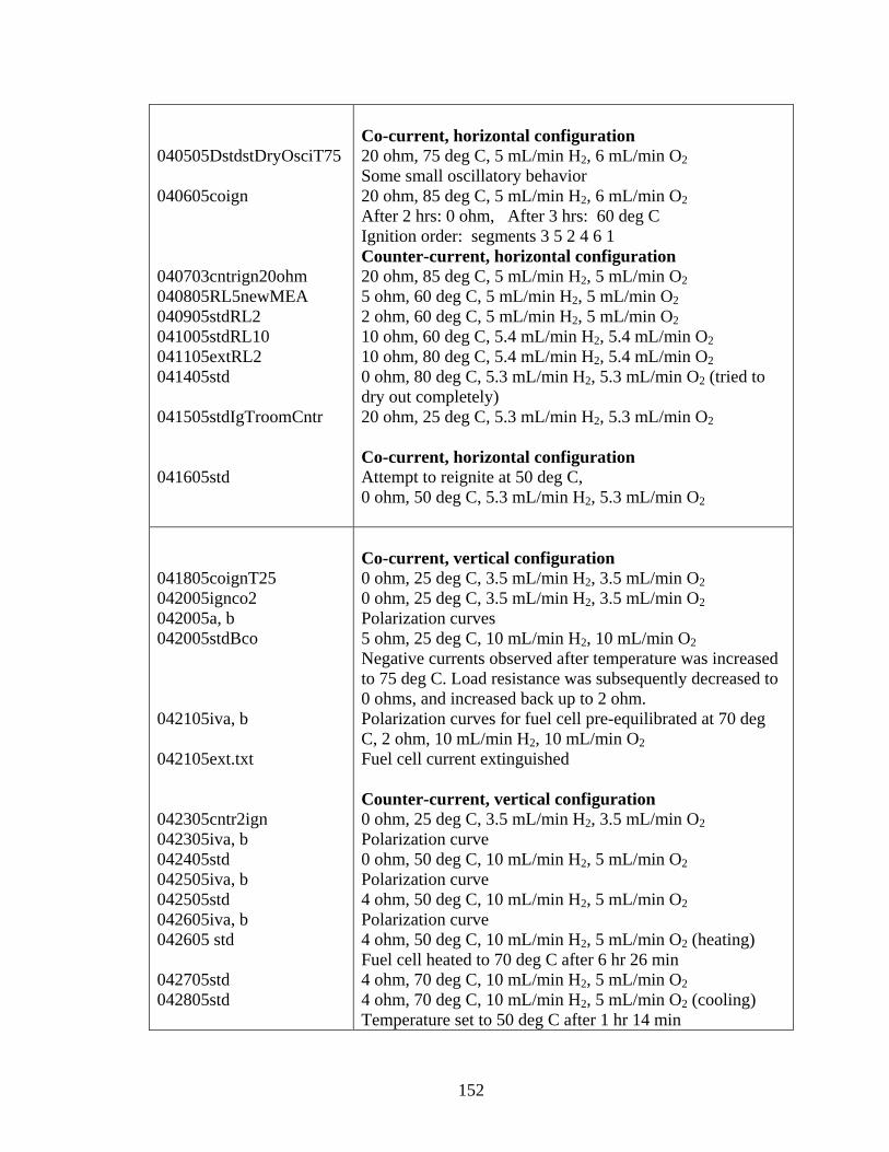
040505DstdstDryOsciT75 040605coign 040703cntrign20ohm 040805RL5newMEA 040905stdRL2 041005stdRL10 041105extRL2 041405std 041505stdIgTroomCntr 041605std
Co-current, horizontal configuration 20 ohm, 75 deg C, 5 mL/min H2, 6 mL/min O2 Some small oscillatory behavior 20 ohm, 85 deg C, 5 mL/min H2, 6 mL/min O2 After 2 hrs: 0 ohm, After 3 hrs: 60 deg C Ignition order: segments 3 5 2 4 6 1 Counter-current, horizontal configuration 20 ohm, 85 deg C, 5 mL/min H2, 5 mL/min O2 5 ohm, 60 deg C, 5 mL/min H2, 5 mL/min O2 2 ohm, 60 deg C, 5 mL/min H2, 5 mL/min O2 10 ohm, 60 deg C, 5.4 mL/min H2, 5.4 mL/min O2 10 ohm, 80 deg C, 5.4 mL/min H2, 5.4 mL/min O2 0 ohm, 80 deg C, 5.3 mL/min H2, 5.3 mL/min O2 (tried to dry out completely) 20 ohm, 25 deg C, 5.3 mL/min H2, 5.3 mL/min O2
Co-current, horizontal configuration Attempt to reignite at 50 deg C, 0 ohm, 50 deg C, 5.3 mL/min H2, 5.3 mL/min O2
041805coignT25 042005ignco2 042005a, b 042005stdBco 042105iva, b 042105ext.txt 042305cntr2ign 042305iva, b 042405std 042505iva, b 042505std 042605iva, b 042605 std 042705std 042805std
Co-current, vertical configuration 0 ohm, 25 deg C, 3.5 mL/min H2, 3.5 mL/min O2 0 ohm, 25 deg C, 3.5 mL/min H2, 3.5 mL/min O2 Polarization curves 5 ohm, 25 deg C, 10 mL/min H2, 10 mL/min O2 Negative currents observed after temperature was increased to 75 deg C. Load resistance was subsequently decreased to 0 ohms, and increased back up to 2 ohm. Polarization curves for fuel cell pre-equilibrated at 70 deg C, 2 ohm, 10 mL/min H2, 10 mL/min O2 Fuel cell current extinguished Counter-current, vertical configuration 0 ohm, 25 deg C, 3.5 mL/min H2, 3.5 mL/min O2 Polarization curve 0 ohm, 50 deg C, 10 mL/min H2, 5 mL/min O2 Polarization curve 4 ohm, 50 deg C, 10 mL/min H2, 5 mL/min O2 Polarization curve 4 ohm, 50 deg C, 10 mL/min H2, 5 mL/min O2 (heating) Fuel cell heated to 70 deg C after 6 hr 26 min 4 ohm, 70 deg C, 10 mL/min H2, 5 mL/min O2 4 ohm, 70 deg C, 10 mL/min H2, 5 mL/min O2 (cooling) Temperature set to 50 deg C after 1 hr 14 min
152

042905std 050105std 050205std 050305std 050605std 050805std 050905stda 051005std 051105iva, b 051105stdA 051105stdB 051205std 051305std 051505std 051605std 051705std
Counter-current, vertical configuration 1 ohm, 50 deg C, 10 mL/min H2, 5 mL/min O2 VwA=6 mL, VwC=6 mL – initial liquid volume Measured the volume of liquid produced from each outlet VwA=8.2 mL, VwC=10.3 mL 1 ohm, 50 deg C, 10 mL/min H2, 5 mL/min O2 VwA=5 mL, VwC=5 mL – initial liquid volume VwA=5.8 mL, VwC=6.5 mL 1 ohm, 70 deg C, 5 mL/min H2, 5 mL/min O2 VwA=5 mL, VwC=5 mL – initial liquid volume VwA=6.3 mL, VwC=6.5 mL Switched graphite pieces an copper backing 20 ohm, 50 deg C, 5 mL/min H2, 5 mL/min O2 Fuel cell current extinguished Cooled to room temperature 3.5 mL/min H2, 3.5 mL/min O2 Swapped out MEA, resumed operation at previous conditions 25 deg C, 5 mL/min H2, 5 mL/min O2 Load resistance increased periodically to extinguish the fuel cell current Polarization curves 0 ohm, 45 deg C, 5 mL/min H2, 5 mL/min O2 Load increased to 20 ohm after 4 hours 0 ohm, 55 deg C, 5 mL/min H2, 5 mL/min O2 Load increased to 20 ohm after 18 hours Current in segments 1 thru 3 much larger than 4 thru 6 Current did not extinguish 0 ohm, 65 deg C, 5 mL/min H2, 5 mL/min O2 Load increased to 20 ohm after 14 hours Current not extinguished 0 ohm, 65 deg C, 5 mL/min H2, 5 mL/min O2 Oscillatory behavior attributed to plugs of water flowing out of the fuel cell periodically. 0 ohm, 70 deg C, 5 mL/min H2, 5 mL/min O2 Load increased to 20 ohm after 15 hours Current did not extinguish completely Counter-current, flat configuration (cathode on top) 0 ohm, 60 deg C, 5 mL/min H2, 5 mL/min O2 0 ohm, 70 deg C, 10 mL/min H2, 5 mL/min O2 5:25pm – VwA=6.8 mL, VwC=5.8 mL 10:00am – VwA=8.9 mL, VwC=6.5 mL
153

051805std 051905std 052105std 052205std 052305iva, b 052305std 052305stdCO 052405stdCO 052405stdB 052505std 052605std 052605stdB 052605stdC 053005std 053105std 060205std 060305std 060505std, 060605std 060705std
Counter-current, vertical configuration 2 ohm, 75 deg C, 9.8 mL/min H2, 5 mL/min O2 Oxygen flow increased to 9 mL/min after 3 hrs 1:55pm – VwA=5.7 mL, VwC=5.2 mL 11:51am – VwA=8.9 mL, VwC=10 mL 6 ohm, 75 deg C, 10 mL/min H2, 10 mL/min O2 4 ohm, 50 deg C, 9 mL/min H2, 9 mL/min O2 4 ohm, 50 deg C, 9.2 mL/min H2, 4.6 mL/min O2 10:55am – VwA=5.2 mL, VwC=5.2 mL 9:50am – VwA=5.9 mL, VwC=5.5 mL 5 ohm, 50 deg C, 9.2 mL/min H2, 9.3 mL/min O2 Co-current, vertical configuration 5 ohm, 50 deg C, 9.2 mL/min H2, 9.3 mL/min O2 t = 0 – VwA=6.0 mL, VwC=7.0 mL t = 17 hr 40 min – VwA=6.4 mL, VwC=7.1 mL 5 ohm, 65 deg C, 9.2 mL/min H2, 9.2 mL/min O2 5 ohm, 60 deg C, 5 mL/min H2, 5 mL/min O2 t = 0 – VwA=6.5 mL, VwC=7.1 mL t =17.5 hr– VwA=6.9 mL, VwC=7.4 mL 5 ohm, 60 deg C, 3.5 mL/min H2, 3.5 mL/min O2 t = 0 – VwA=6.9 mL, VwC=7.4 mL t =23 hr – VwA=7.5 mL, VwC=7.8 mL 5 ohm, 60 deg C, 9.2 mL/min H2, 9.2 mL/min O2 t = 0 – VwA= 5 mL, VwC= 5 mL t =7.5 hr – VwA=5.1 mL, VwC=5 mL 5 ohm, 70 deg C, 9.2 mL/min H2, 9.3 mL/min O2 t = 0 – VwA=5.1 mL, VwC=5.0 mL t =6.5 hr – VwA=5.25 mL, VwC=5.05 mL 5 ohm, 25 deg C, 9.2 mL/min H2, 9.2 mL/min O2 t = 0 – VwA=5.25 mL, VwC=5.0 mL t = 11 hr – VwA=5.3 mL, VwC=5.15 mL 5 ohm, 40 deg C, 9.2 mL/min H2, 9.3 mL/min O2 t = 0 – VwA=5.65 mL, VwC=6.15 mL t =23.5 hr – VwA=6.05 mL, VwC=6.40 mL 5 ohm, 35 deg C, 9.2 mL/min H2, 9.3 mL/min O2 t = 0 – VwA=6.05 mL, VwC=6.40 mL t =6.5 hr – VwA=6.35 mL, VwC=6.60 mL Counter-current, vertical configuration 5 ohm, 25 deg C, 9.2 mL/min H2, 9.3 mL/min O2 5 ohm, 25 deg C, 9.2 mL/min H2, 9.3 mL/min O2 t = 0 – VwA=3.95 mL, VwC=5.0 mL t = 21 hr – VwA=4.15 mL, VwC=5.9 mL 5 ohm, 40 deg C, 9.2 mL/min H2, 9.3 mL/min O2 5 ohm, 50 deg C, 9.2 mL/min H2, 9.3 mL/min O2
154

155
060805std 060905std 061005std 061305std 061505std 062005std 062105
t = 0 – VwA=4.9 mL, VwC=6.2 mL t = 28.5 hr – VwA=5.3 mL, VwC=6.5 mL 5 ohm, 60 deg C, 9.2 mL/min H2, 9.3 mL/min O2 t = 0 – VwA=5.0 mL, VwC=6.5 mL t = 25 hr – VwA=5.3 mL, VwC=6.6 mL 5 ohm, 70 deg C, 9.2 mL/min H2, 9.3 mL/min O2 t = 0 – VwA=5.3 mL, VwC=6.6 mL t = 23 hr – VwA=5.8 mL, VwC=6.9 mL 5 ohm, 70 deg C, 9.2 mL/min H2, 9.3 mL/min O2 t = 0 – VwA=5.0 mL, VwC=5.0 mL t = 2 days – VwA=6.0 mL, VwC=5.2 mL Co-current, vertical configuration 5 ohm, 25 deg C, 9.2 mL/min H2, 9.3 mL/min O2 t = 0 – VwA=6.1 mL, VwC=5.95 mL 5 ohm, 25 deg C, 9.2 mL/min H2, 9.3 mL/min O2 t = 5 days – VwA=6.5 mL, VwC=8.3 mL 5 ohm, 40 deg C, 9.2 mL/min H2, 9.3 mL/min O2 t = 0 – VwA=5.5 mL, VwC=5.5 mL t =23 hr – VwA=5.9 mL, VwC=5.9 mL 5 ohm, 50 deg C, 9.2 mL/min H2, 9.3 mL/min O2