EE 6161

EE 616 Computer Aided Analysis of Electronic Networks

Lecture 2

Instructor: Dr. J. A. Starzyk, ProfessorSchool of EECSOhio UniversityAthens, OH, 45701

EE 6162

Review and Outline

Review of the previous lecture

-- Class organization

-- CAD overview Outline of this lecture

* Review of network scaling

* Review of Thevenin/Norton Analysis

* Formulation of Circuit Equations

-- KCL, KVL, branch equations

-- Sparse Tableau Analysis (STA)

-- Nodal analysis

-- Modified nodal analysis

EE 6163

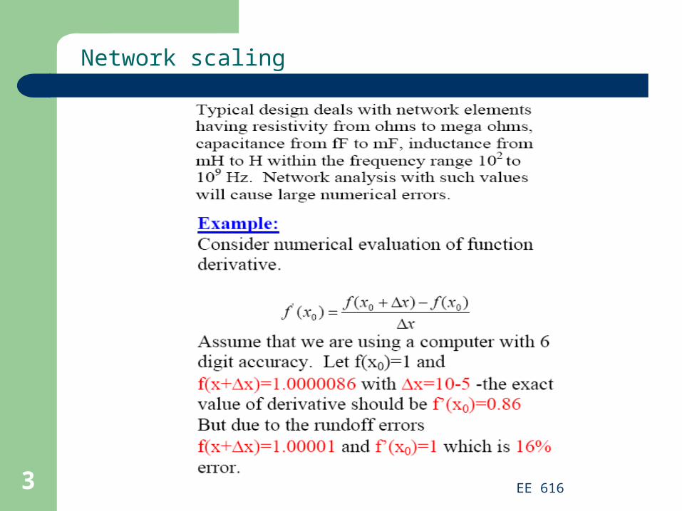
Network scaling

EE 6164

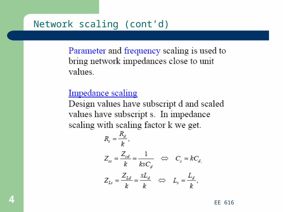
Network scaling (cont’d)

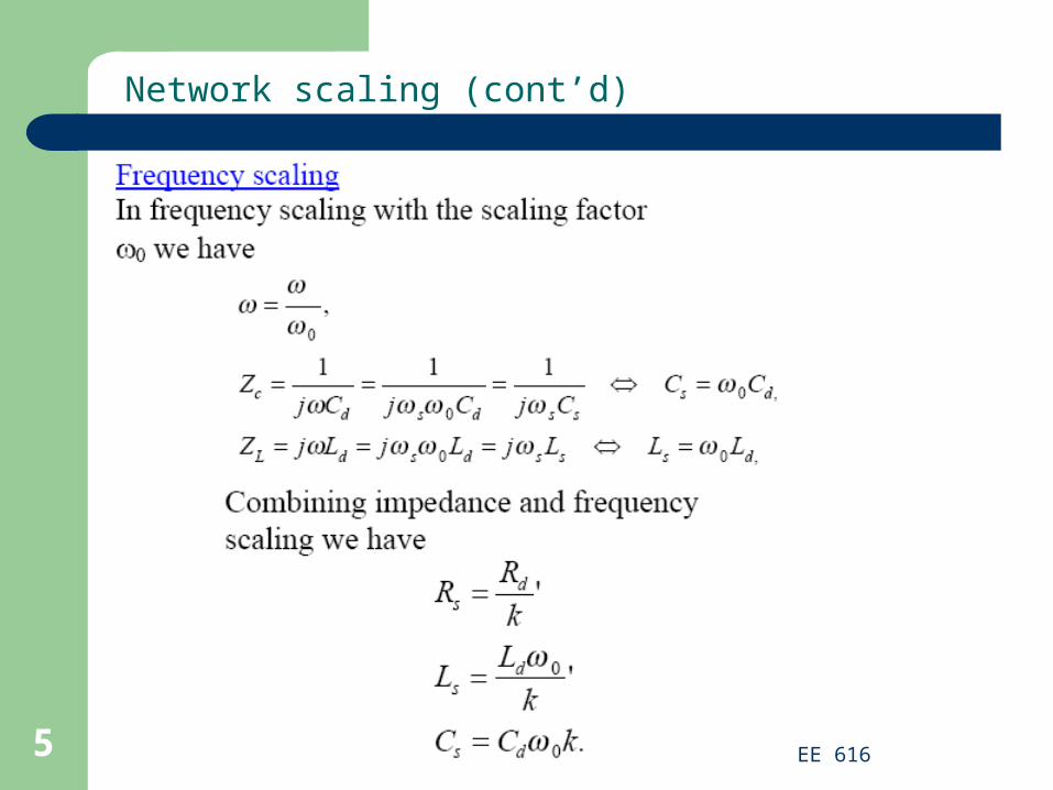
EE 6165

Network scaling (cont’d)

EE 6166

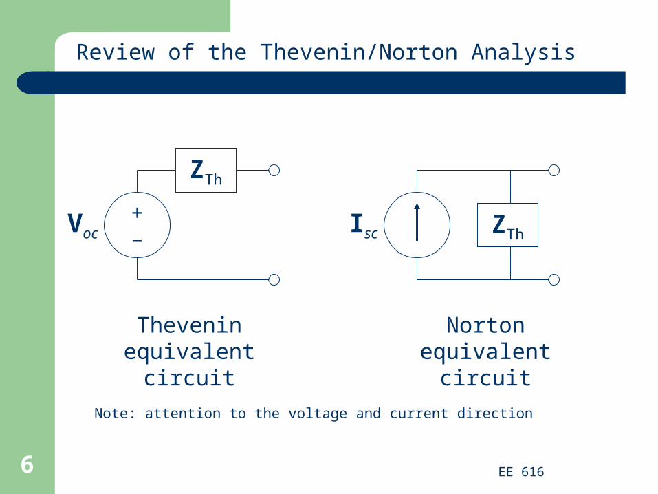
Voc

Thevenin equivalent circuit

ZTh

+–

Norton equivalent circuit

ZThIsc

Note: attention to the voltage and current direction

Review of the Thevenin/Norton Analysis

EE 6167

1. Pick a good breaking point in the circuit (cannot split a dependent source and its control variable).

2.Replace the load by either an open circuit and calculate the voltage E across the terminals A-A’, or a short circuit A-A’ and calculate the current J flowing into the short circuit. E will be the value of the source of the Thevenin equivalent and J that of the Norton equivalent.

3. To obtain the equivalent source resistance, short-circuit all independent voltage sources and open-circuit all independent current sources. Transducers in the network are left unchanged. Apply a unit voltage source (or a unit current source) at the terminals A-A’ and calculate the current I supplied by the voltage source (voltage V

across the current source). The Rs = 1/I (Rs = V).

Review of the Thevenin/Norton Analysis

EE 6168

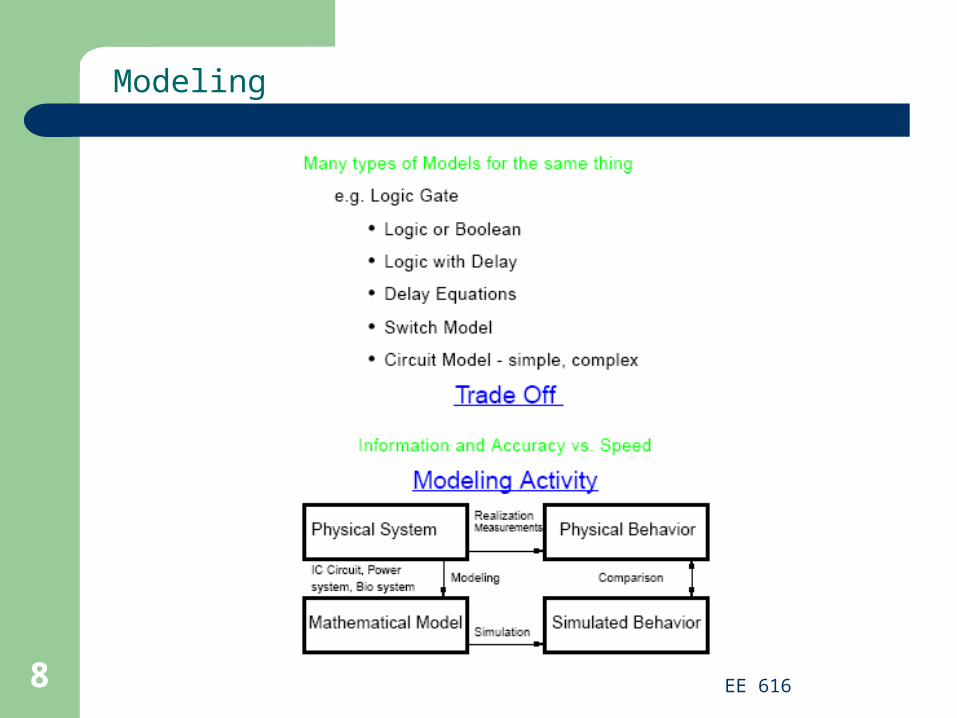
Modeling

EE 6169

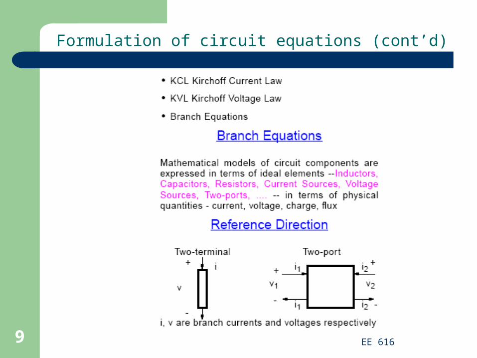
Formulation of circuit equations (cont’d)

EE 61610

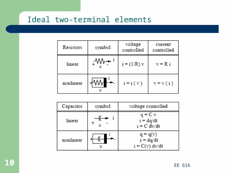
Ideal two-terminal elements

EE 61611

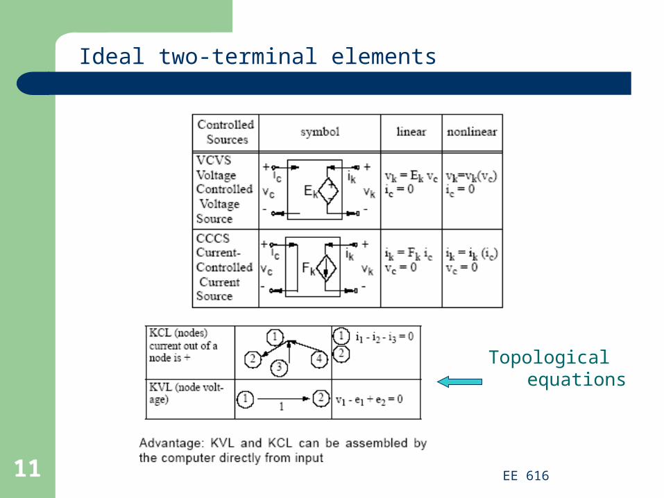
Ideal two-terminal elements

Topological equations

EE 61612

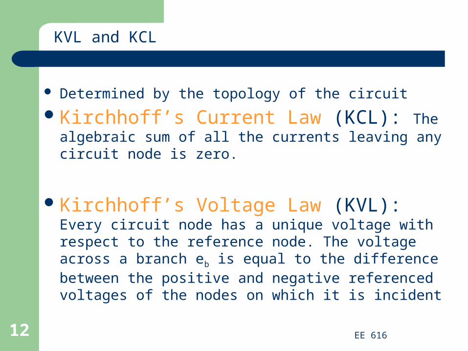
Determined by the topology of the circuit

Kirchhoff’s Current Law (KCL): The algebraic sum of all the currents leaving any circuit node is zero.

Kirchhoff’s Voltage Law (KVL): Every circuit node has a unique voltage with respect to the reference node. The voltage across a branch eb is equal to the difference between the positive and negative referenced voltages of the nodes on which it is incident

KVL and KCL

EE 61613

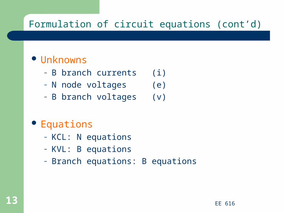
Unknowns– B branch currents (i)– N node voltages (e)– B branch voltages (v)

Equations– KCL: N equations– KVL: B equations– Branch equations: B equations

Formulation of circuit equations (cont’d)

EE 61614

Determined by the mathematical model of the electrical behavior of a component– Example: V=R·I

In most of circuit simulators this mathematical model is expressed in terms of ideal elements

Branch equations

EE 61615

Matrix form of KVL and KCL

N equations

B equations

EE 61616

55

4

3

2

1

5

4

3

2

1

4

3

2

1

0

0

0

0

00000

01

000

001

00

0000

00001

sii

i

i

i

i

v

v

v

v

v

R

R

GR

Kvv + i = is B equations

Branch equation

EE 61617

1 2 3 j B

12

i

N

branches

nodes (+1, -1, 0)

{Aij = +1 if node i is terminal + of branch j-1 if node i is terminal - of branch j0 if node i is not connected to branch j

PROPERTIES•A is unimodular•2 nonzero entries in each column

Node branch incidence matrix

EE 61618

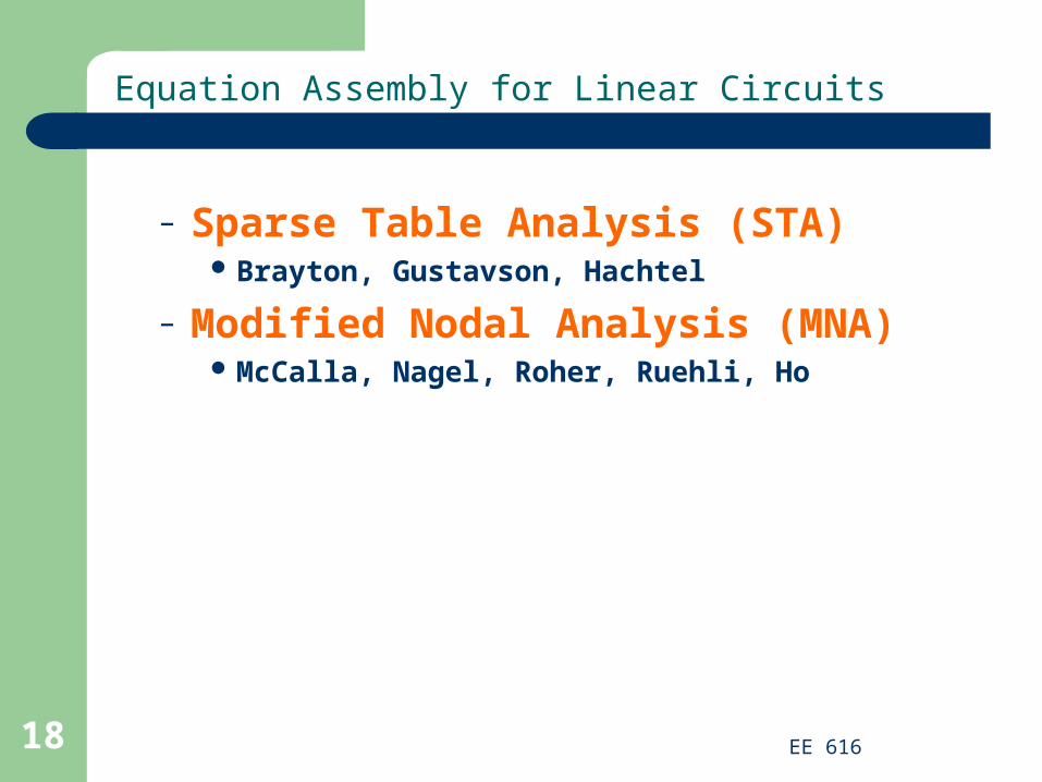
– Sparse Table Analysis (STA) Brayton, Gustavson, Hachtel

– Modified Nodal Analysis (MNA) McCalla, Nagel, Roher, Ruehli, Ho

Equation Assembly for Linear Circuits

EE 61619

Sparse Tableau Analysis (STA)

EE 61620

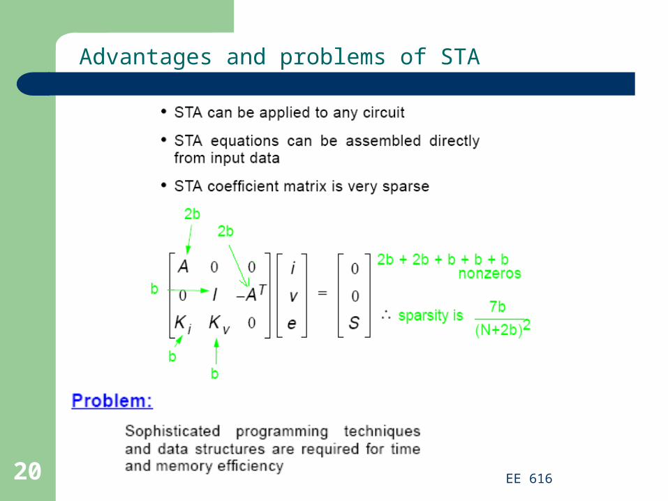
Advantages and problems of STA

EE 61621

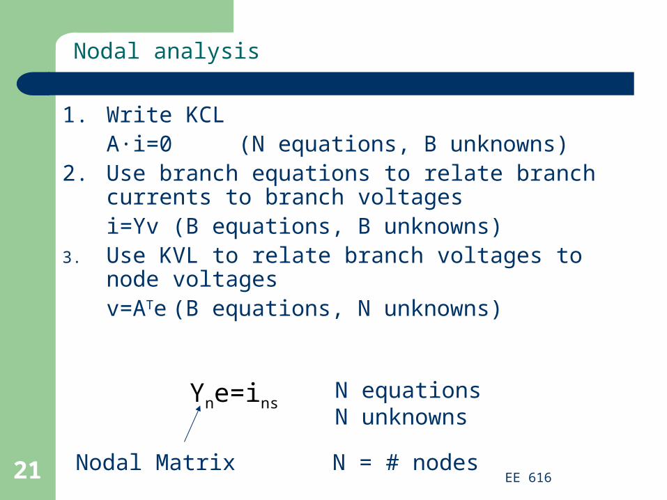
1. Write KCLA·i=0 (N equations, B unknowns)

2. Use branch equations to relate branch currents to branch voltagesi=Yv (B equations, B unknowns)

3. Use KVL to relate branch voltages to node voltagesv=ATe (B equations, N unknowns)

Yne=insN equationsN unknowns

N = # nodesNodal Matrix

Nodal analysis

EE 61622

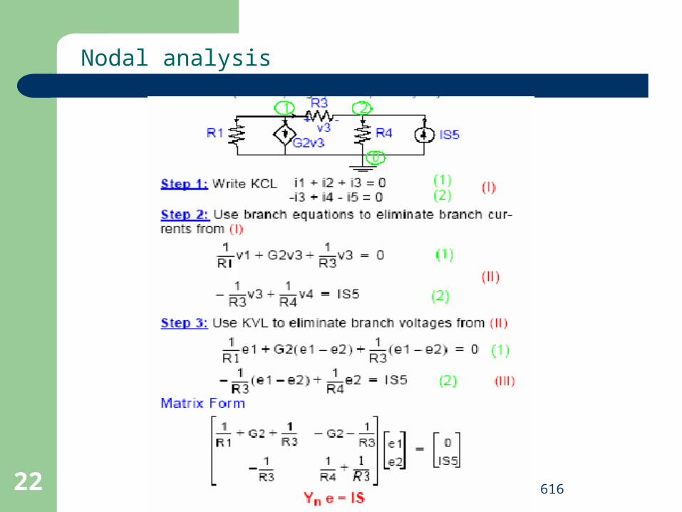
Nodal analysis

EE 61623

Spice input format: Rk N+ N- Rkvalue

kk

kk

RR

RR11

11N+ N-

N+

N-

N+

N-

iRk

sNNk

others

sNNk

others

ieeR

i

ieeR

i

1

1KCL at node N+

KCL at node N-

Nodal analysis – Resistor “Stamp”

EE 61624

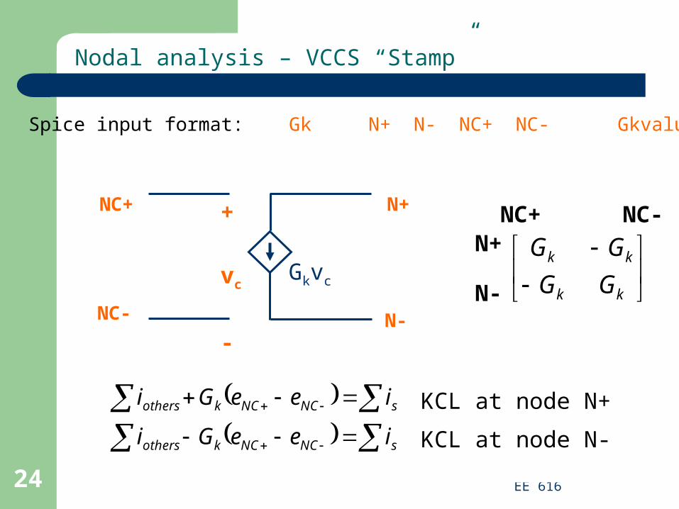
Spice input format: Gk N+ N- NC+ NC- Gkvalue

kk

kk

GG

GGNC+ NC-

N+

N-

N+

N-

Gkvc

NC+

NC-

+

vc

-

sNCNCkothers

sNCNCkothers

ieeGi

ieeGi KCL at node N+

KCL at node N-

Nodal analysis – VCCS “Stamp”

EE 61625

Nodal analysis- independent current sources “stamp”

EE 61626

Rules (page 36):

1. The diagonal entries of Y are positive and

admittances connected to node j

2. The off-diagonal entries of Y are negative and are given by

admittances connected between nodes j and k

3. The jth entry of the right-hand-side vector J is

currents from independent sources entering node j

Nodal analysis- by inspection

jky

jjy

jJ

EE 61627

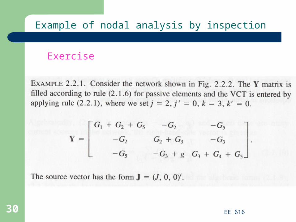
Example of nodal analysis by inspection

ExerciseFormulate nodal equations by inspection

EE 61628

Example of nodal analysis by inspection

EE 61629

Example of nodal analysis by inspection

ExerciseFormulate nodal equations by inspection

EE 61630

Example of nodal analysis by inspection

Exercise

EE 61631

Nodal analysis (cont’d)

EE 61632

Modified Nodal Analysis (MNA)

EE 61633

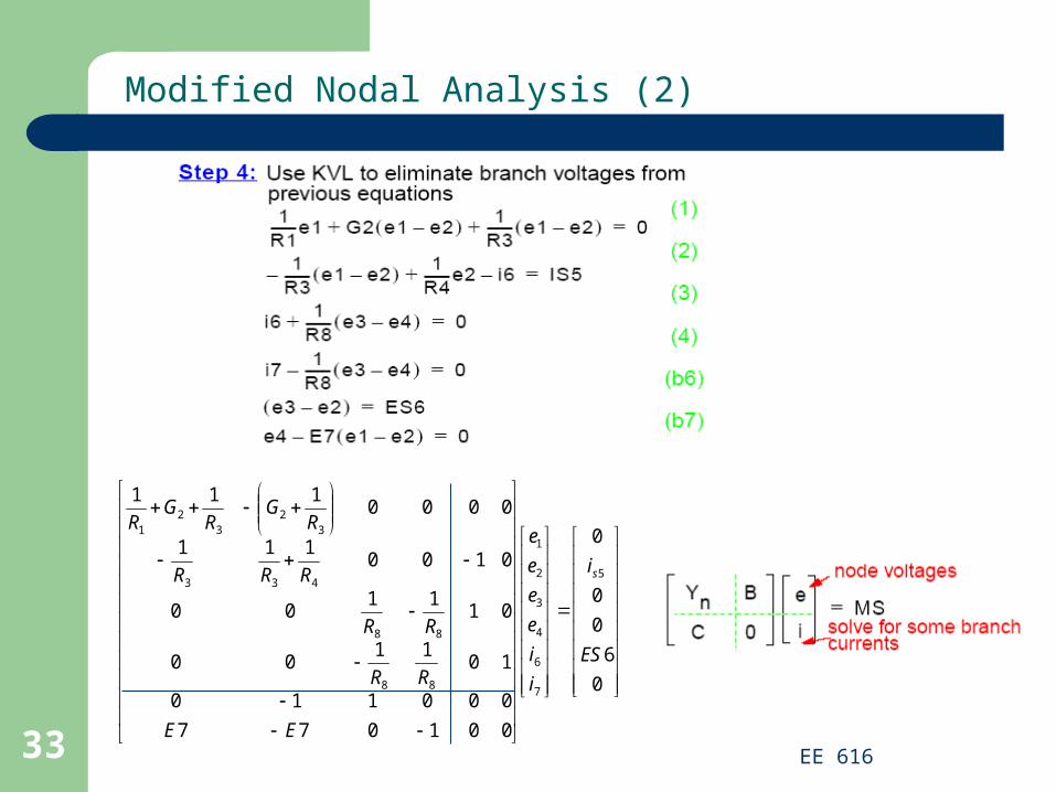
Modified Nodal Analysis (2)

0

6

0

0

0

001077

000110

1011

00

0111

00

0100111

0000111

5

7

6

4

3

2

1

88

88

433

32

32

1

ES

i

i

i

e

e

e

e

EE

RR

RR

RRR

RG

RG

R

s

EE 61634

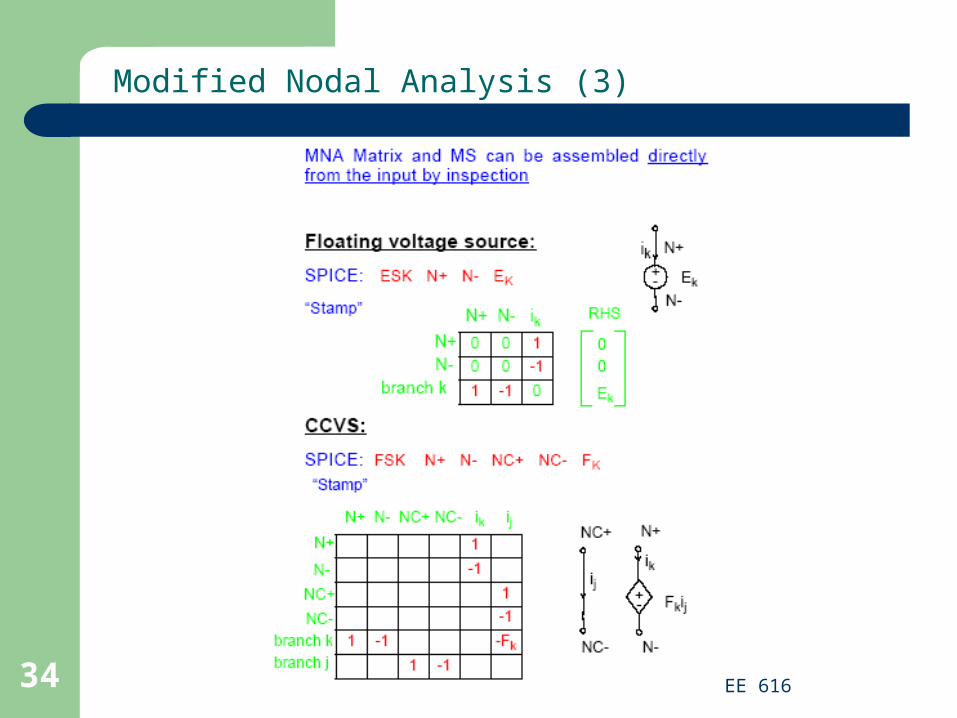
Modified Nodal Analysis (3)

EE 61635

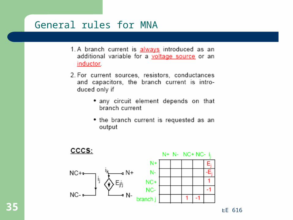
General rules for MNA

EE 61636

Example 4.4.1(p.143)

EE 61637

Advantages and problems of MNA

EE 61638

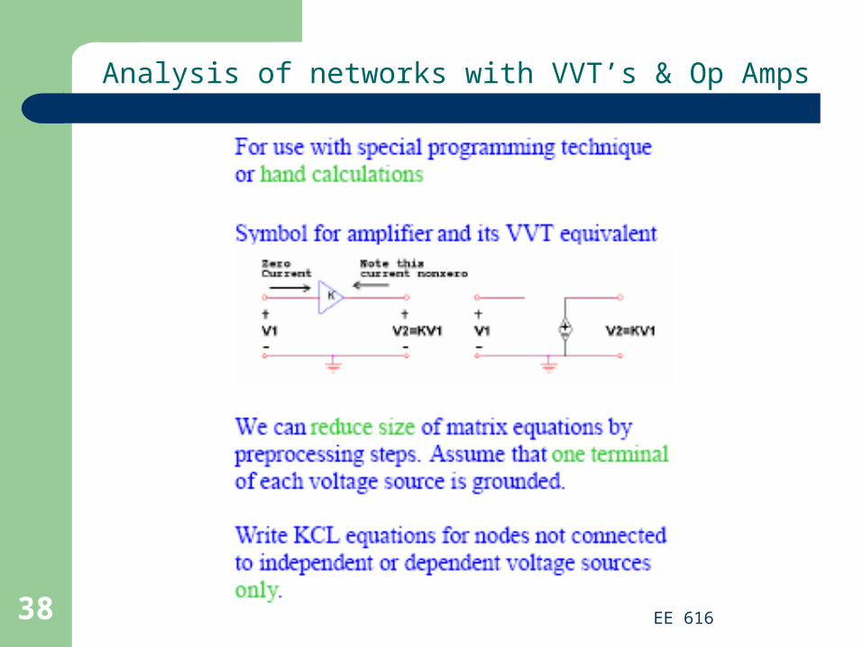
Analysis of networks with VVT’s & Op Amps

EE 61639

Example 4.5.2 (p.145)

EE 61640

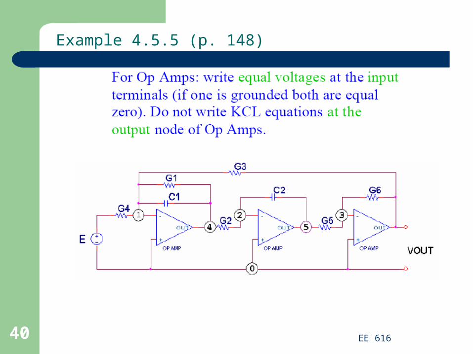
Example 4.5.5 (p. 148)

EE 61641

Example 4.5.5 (cont’d)