ee 508 lecture 2 - iowa state universityclass.ece.iastate.edu/ee508/lectures/ee 508 lect 16 fall...
TRANSCRIPT

EE 508
Lecture 16
Filter Transformations
Lowpass to Bandpass
Lowpass to Highpass
Lowpass to Band-reject
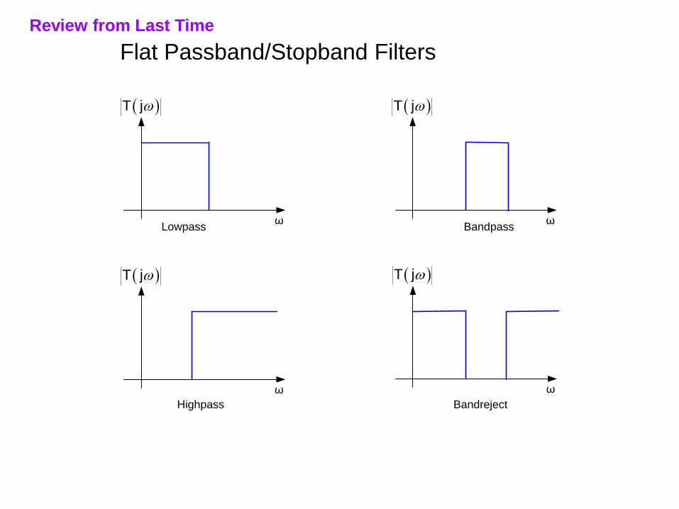
Flat Passband/Stopband Filters
ω
T j
ω
T j
ω
T j
ω
T j
Lowpass Bandpass
Highpass Bandreject
Review from Last Time
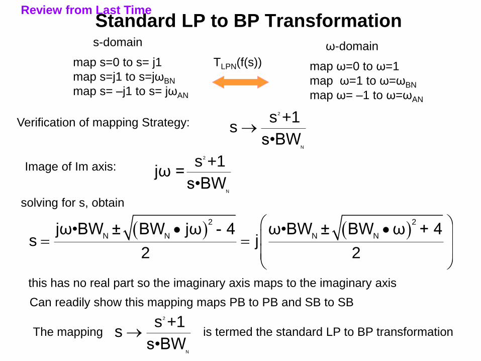
Standard LP to BP Transformation
Verification of mapping Strategy:2
N
s +1s
s•BW
The mapping is termed the standard LP to BP transformation
2
N
s +1s
s•BW
map s=0 to s= j1
map s=j1 to s=jωBN
map s= –j1 to s= jωAN
map ω=0 to ω=1
map ω=1 to ω=ωBN
map ω= –1 to ω=ωAN
s-domain ω-domain
TLPN(f(s))
Image of Im axis:2
N
s +1jω =
s•BW
2 2
N N N Njω•BW ± BW jω - 4 ω•BW ± BW ω + 4
s j2 2
solving for s, obtain
this has no real part so the imaginary axis maps to the imaginary axis
Can readily show this mapping maps PB to PB and SB to SB
Review from Last Time
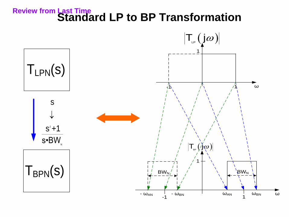
Standard LP to BP Transformation
ω
1
1
ω
1
1
ωAN ωBN
LP
T j
BP
T j
BWN
-1
-1- ωAN - ωBN
BWN
TLPN(s)
TBPN(s)
2
N
s
s +1
s•BW
Review from Last Time
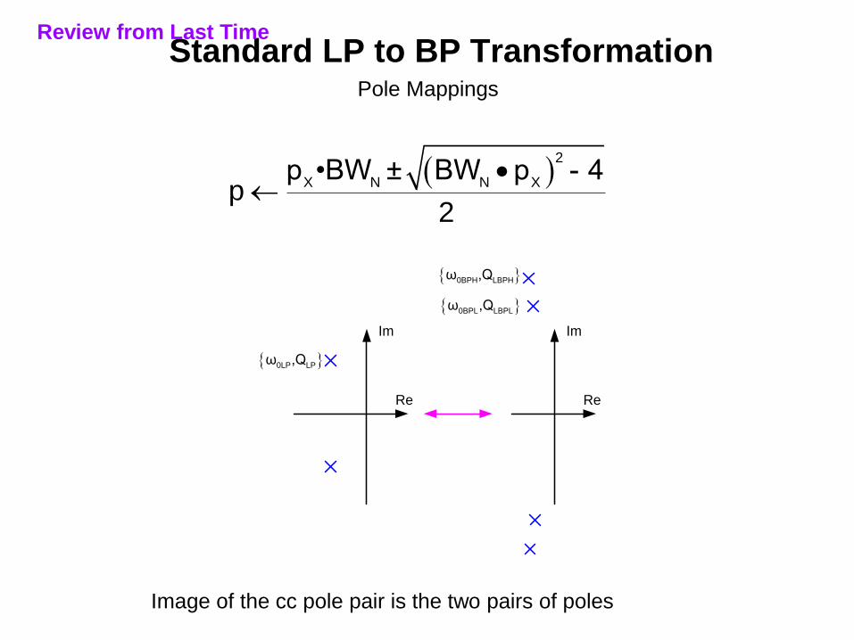
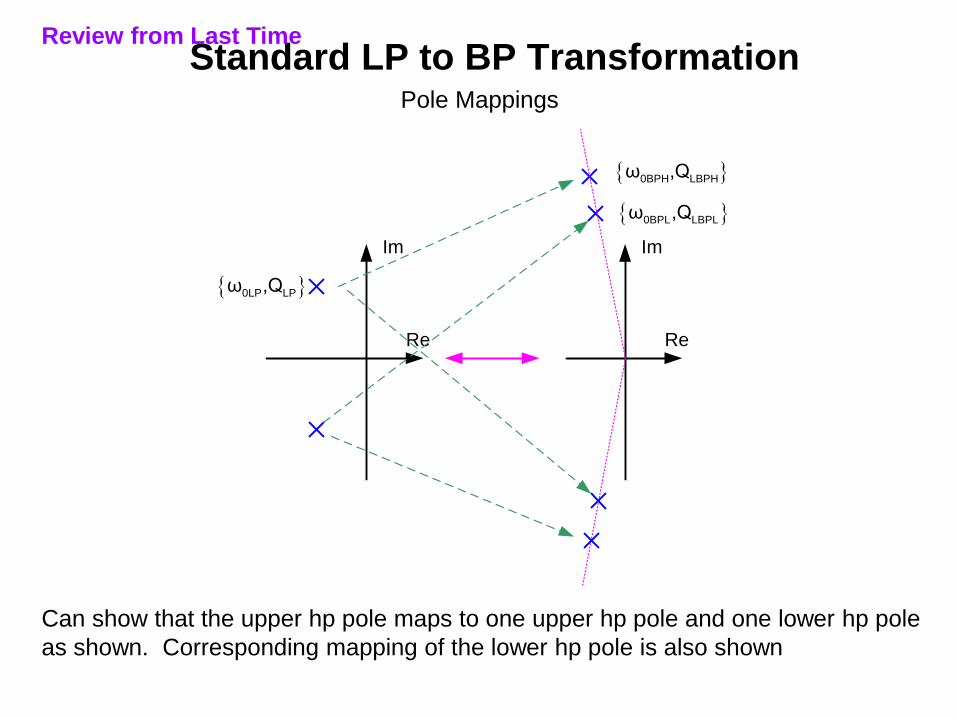
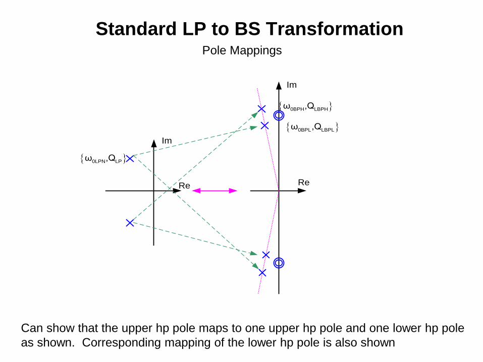
Standard LP to BP TransformationPole Mappings
2
X N N Xp •BW ± BW p - 4
p2
Re
Im
Re
Im
0BPH LBPHω ,Q
0LP LPω ,Q
0BPL LBPLω ,Q
Image of the cc pole pair is the two pairs of poles
Review from Last Time
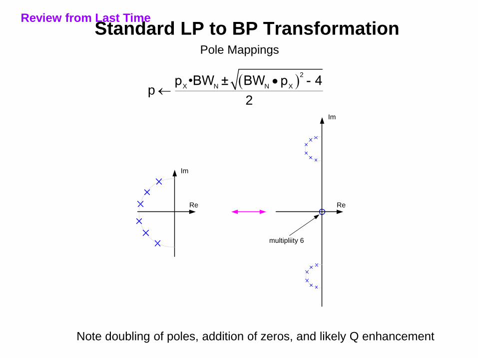
Standard LP to BP TransformationPole Mappings
Can show that the upper hp pole maps to one upper hp pole and one lower hp pole
as shown. Corresponding mapping of the lower hp pole is also shown
Re
Im
Re
Im
0BPH LBPHω ,Q
0LP LPω ,Q
0BPL LBPLω ,Q
Review from Last Time
Standard LP to BP TransformationPole Mappings
2
X N N Xp •BW ± BW p - 4
p2
Re
Im
Re
Im
multipliity 6
Note doubling of poles, addition of zeros, and likely Q enhancement
Review from Last Time
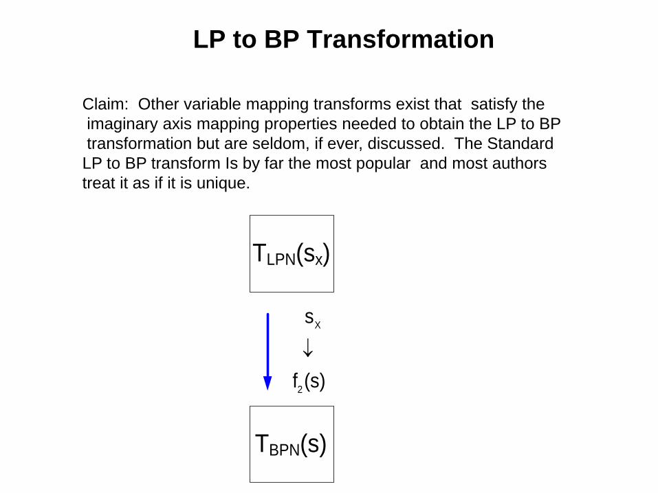
LP to BP Transformation
TLPN(sx)
TBPN(s)
X
2
s
f (s)
Claim: Other variable mapping transforms exist that satisfy the
imaginary axis mapping properties needed to obtain the LP to BP
transformation but are seldom, if ever, discussed. The Standard
LP to BP transform Is by far the most popular and most authors
treat it as if it is unique.
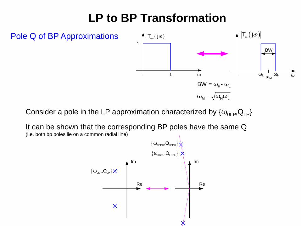
LP to BP Transformation
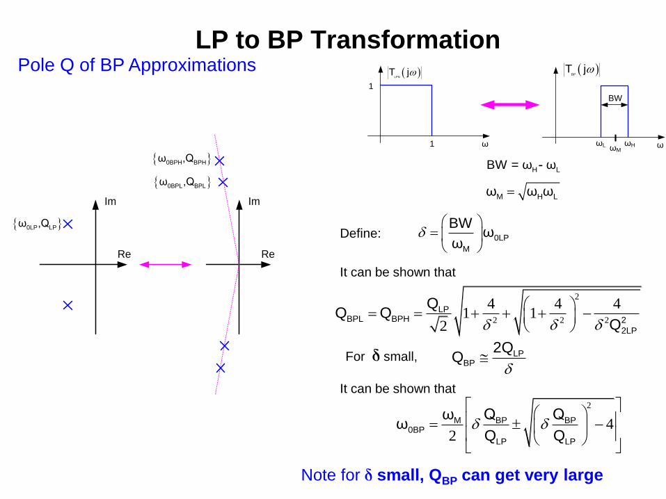
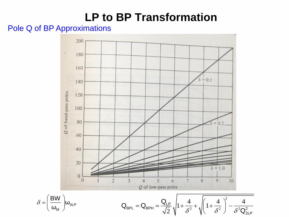
Pole Q of BP Approximations
ω
LPN
T j
ω
BP
T j
1
1
ωM
BW
ωL ωH
H LBW = ω - ω
M H Lω ω ω
Consider a pole in the LP approximation characterized by {ω0LP,QLP}
It can be shown that the corresponding BP poles have the same Q (i.e. both bp poles lie on a common radial line)
Re
Im
Re
Im
0BPH LBPHω ,Q
0LP LPω ,Q
0BPL LBPLω ,Q
LP to BP TransformationPole Q of BP Approximations
Define: 0LP
M
BWω
ω
ω
LPN
T j
ω
BP
T j
1
1
ωM
BW
ωL ωH
H LBW = ω - ω
M H Lω ω ω
Re
Im
Re
Im
0BPH BPHω ,Q
0LP LPω ,Q
0BPL BPLω ,Q
It can be shown that
2
2 2 2
4 4 41 1
2
LPBPL BPH 2
2LP
QQ Q
Q
For d small, LPBP
2QQ
It can be shown that 2
42
M BP BP0BP
LP LP
ω Q Qω
Q Q
Note for d small, QBP can get very large
LP to BP TransformationPole Q of BP Approximations
2
2 2 2
4 4 41 1
2
LPBPL BPH 2
2LP
QQ Q
Q
0LP
M
BWω
ω
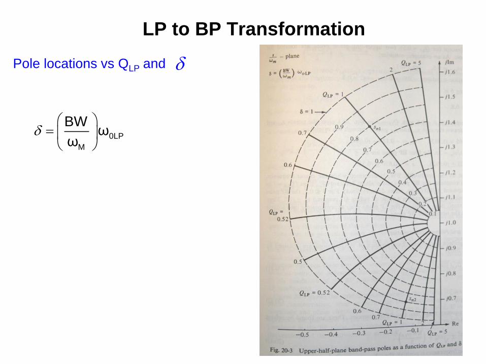
LP to BP Transformation
Pole locations vs QLP and
0LP
M
BWω
ω
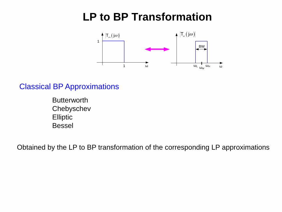
LP to BP Transformation
Classical BP Approximations
ω
LPN
T j
ω
BP
T j
1
1
ωM
BW
ωL ωH
Butterworth
Chebyschev
Elliptic
Bessel
Obtained by the LP to BP transformation of the corresponding LP approximations
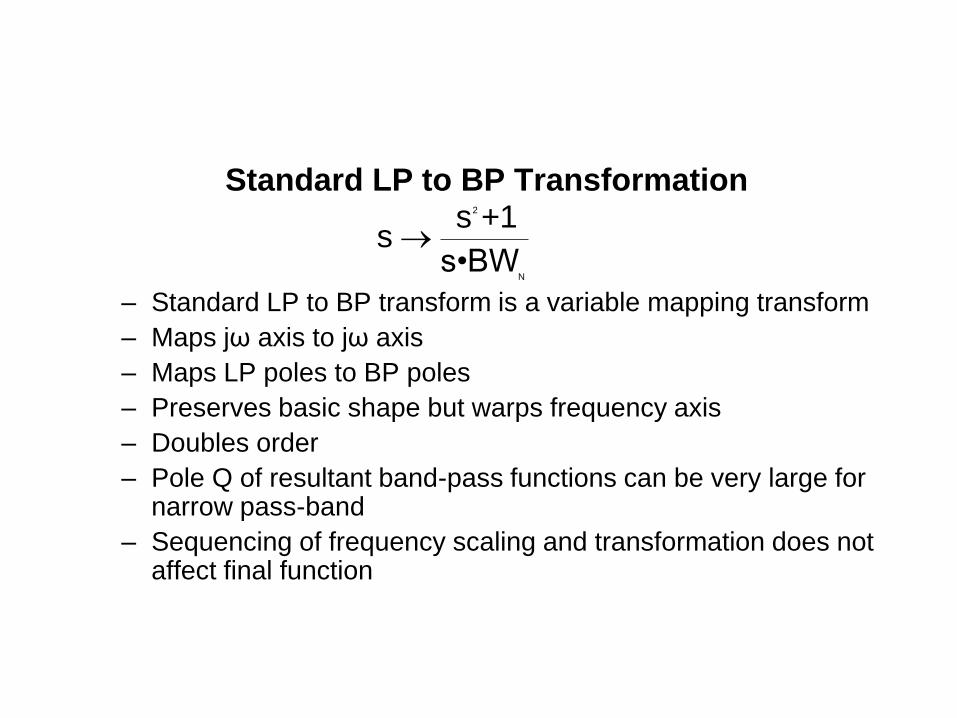
Standard LP to BP Transformation
– Standard LP to BP transform is a variable mapping transform
– Maps jω axis to jω axis
– Maps LP poles to BP poles
– Preserves basic shape but warps frequency axis
– Doubles order
– Pole Q of resultant band-pass functions can be very large for narrow pass-band
– Sequencing of frequency scaling and transformation does not affect final function
2
N
s +1s
s•BW
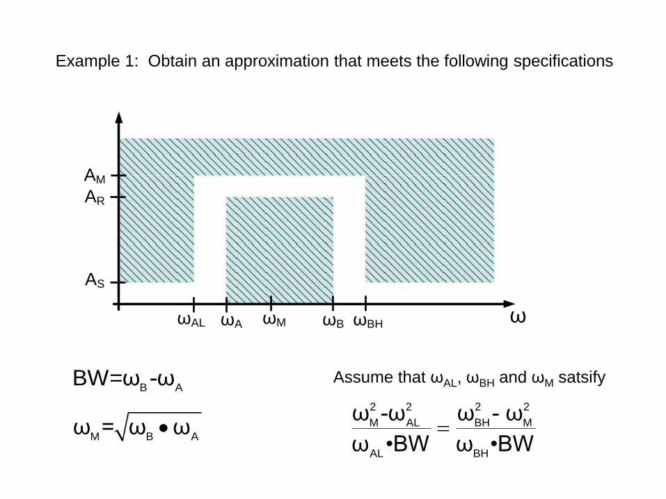
Example 1: Obtain an approximation that meets the following specifications
ω
AM
AR
AS
ωMωA ωB ωBHωAL
2 2 2 2
M AL BH M
AL BH
ω -ω ω - ω
ω •BW ω •BW
B ABW=ω -ω
M B Aω = ω ω
Assume that ωAL, ωBH and ωM satsify
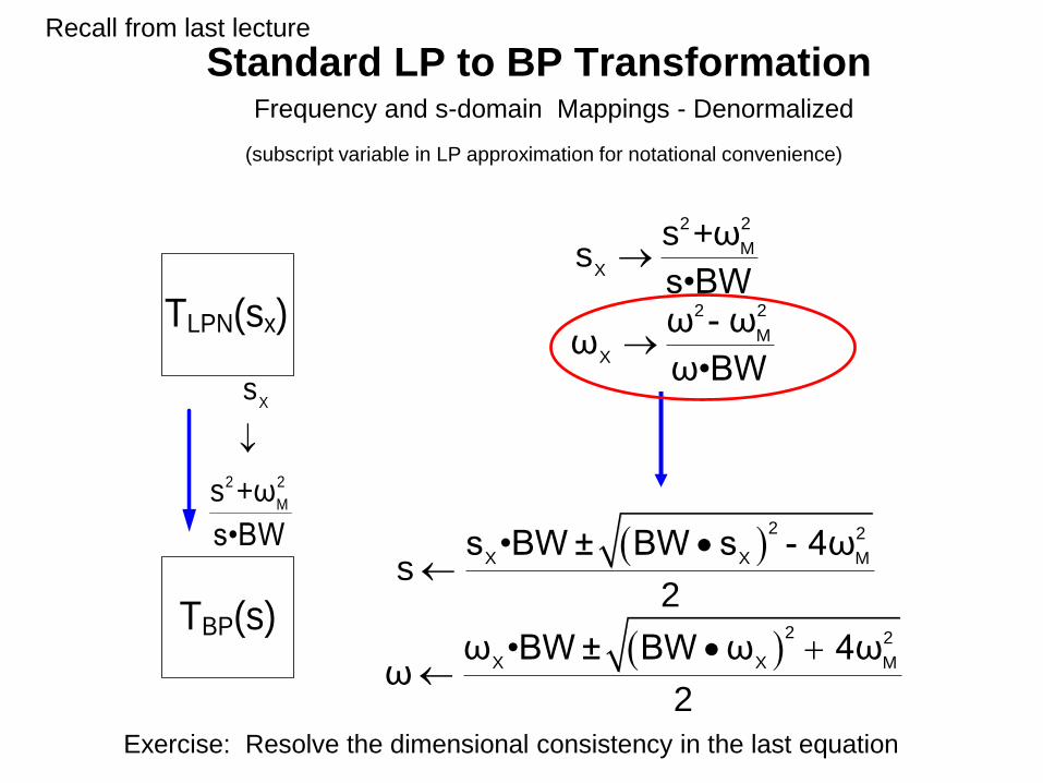
Standard LP to BP TransformationFrequency and s-domain Mappings - Denormalized
(subscript variable in LP approximation for notational convenience)
TLPN(sx)
TBP(s)
X
2 2
M
s
s +ω
s•BW
2 2
M
X
s +ωs
s•BW
2 2
M
X
ω - ωω
ω•BW
2 2
X X Ms •BW ± BW s - 4ω
s2
2 2
X X Mω •BW ± BW ω 4ω
ω2
Exercise: Resolve the dimensional consistency in the last equation
Recall from last lecture
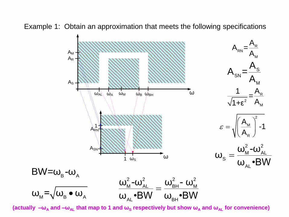
Example 1: Obtain an approximation that meets the following specifications
2 2 2 2
M AL BH M
AL BH
ω -ω ω - ω
ω •BW ω •BW
B ABW=ω -ω
M B Aω = ω ω
R
2M
A1=
A1+ε
2
M
R
A-1
A
R
RN
M
AA =
A
2 2
M AL
S
AL
ω -ω ω
ω •BW
S
SN
M
AA =
A
1 ω
ω
AM
AR
AS
ASN
ωS
ωMωA ωB ωBHωAL
1ARN
(actually –ωA and –ωAL that map to 1 and ωS respectively but show ωA and ωAL for convenience)
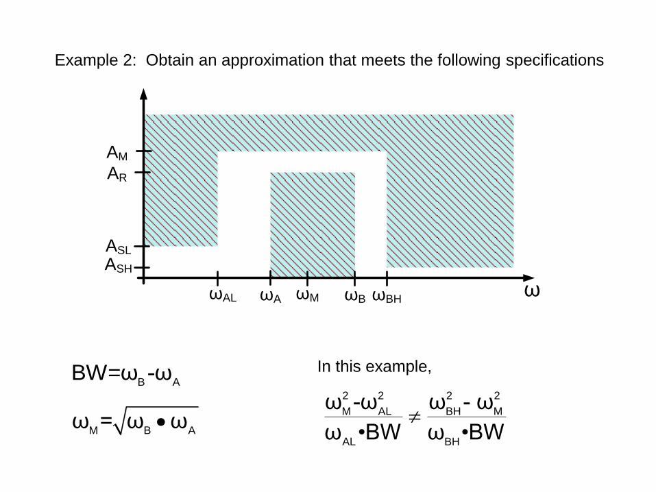
Example 2: Obtain an approximation that meets the following specifications
2 2 2 2
M AL BH M
AL BH
ω -ω ω - ω
ω •BW ω •BW
B ABW=ω -ω
M B Aω = ω ω
ωMωA ωB ωBHωAL ω
AM
AR
ASH
ASL
In this example,
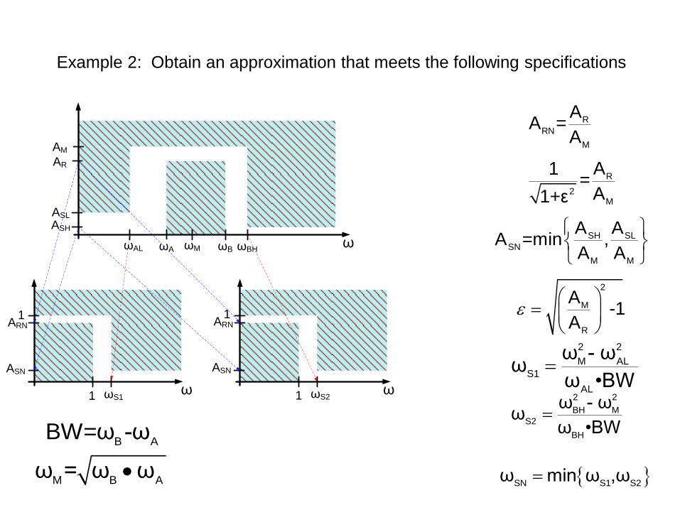
Example 2: Obtain an approximation that meets the following specifications
B ABW=ω -ω
M B Aω = ω ω
ωMωA ωB ωBHωAL ω
ω ω
ASN
1ARN
ASN
1ARN
1 ωS1 1 ωS2
AM
AR
ASH
ASL
R
RN
M
AA =
A
R
2M
A1=
A1+ε
2
M
R
A-1
A
2 2
M AL
S1
AL
ω - ω ω
ω •BW
2 2
BH M
S2
BH
ω - ωω
ω •BW
SH SL
SN
M M
A AA =min ,
A A
SN S1 S2ω min ω ,ω
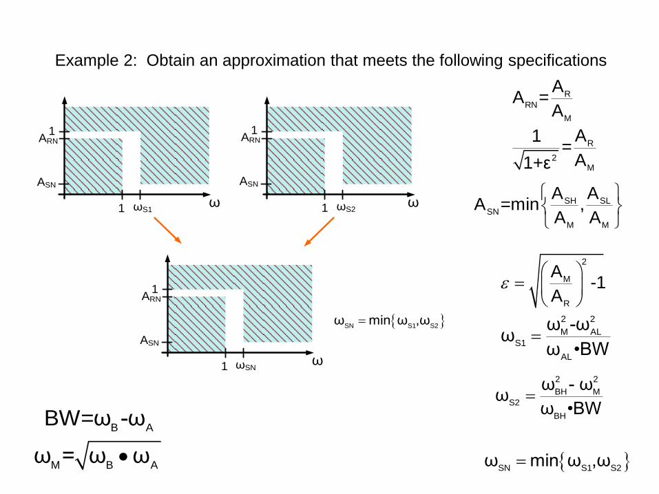
Example 2: Obtain an approximation that meets the following specifications
B ABW=ω -ω
M B Aω = ω ω
R
RN
M
AA =
A
R
2M
A1=
A1+ε
2
M
R
A-1
A
2 2
M AL
S1
AL
ω -ω ω
ω •BW
2 2
BH M
S2
BH
ω - ωω
ω •BW
SH SL
SN
M M
A AA =min ,
A A
SN S1 S2ω min ω ,ω
ω ω
ASN
1ARN
ASN
1ARN
1 ωS1 1 ωS2
ω
ASN
1ARN
1 ωSN
SN S1 S2ω min ω ,ω
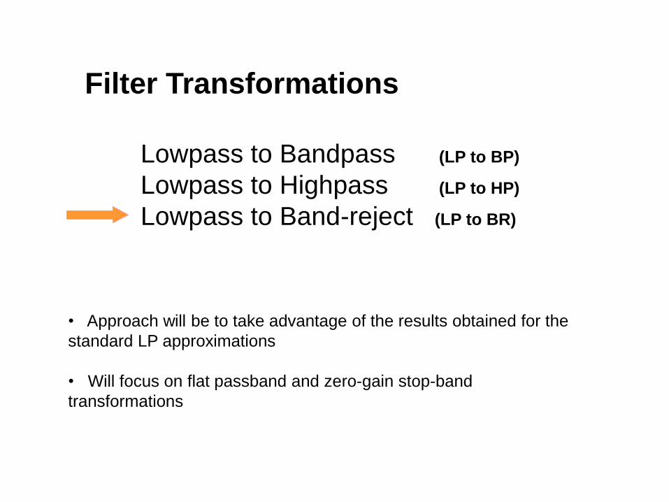
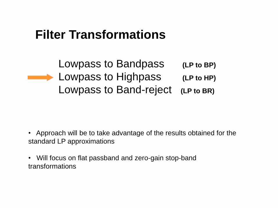
Filter Transformations
Lowpass to Bandpass (LP to BP)
Lowpass to Highpass (LP to HP)
Lowpass to Band-reject (LP to BR)
• Approach will be to take advantage of the results obtained for the
standard LP approximations
• Will focus on flat passband and zero-gain stop-band
transformations
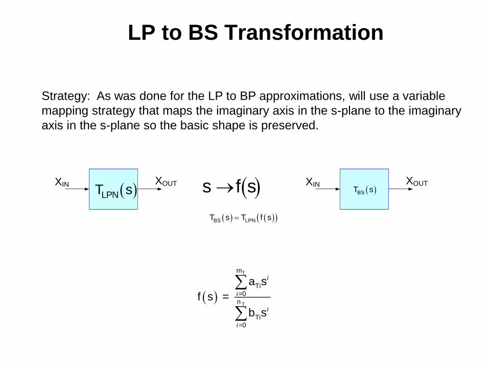
LP to BS Transformation
Strategy: As was done for the LP to BP approximations, will use a variable
mapping strategy that maps the imaginary axis in the s-plane to the imaginary
axis in the s-plane so the basic shape is preserved.
XIN XOUT
LPNT sXIN XOUT
BST s s f s
BS LPNT s T f s
T
T
m
Ti
=0
n
Ti
=0
a s
f s =
b s
i
i
i
i
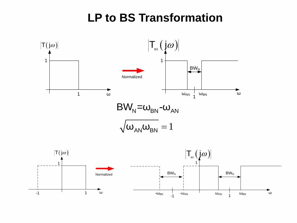
LP to BS Transformation
1
1
ω1
1
ω
T j BS
T j
Normalized
BWN
ωBNωAN
1
1
ω1
1
ω
T j BS
T j
Normalized
-1-1
BWNBWN
ωBN-ωBN ωAN-ωAN
N BN ANBW =ω -ω
1AN BNω ω
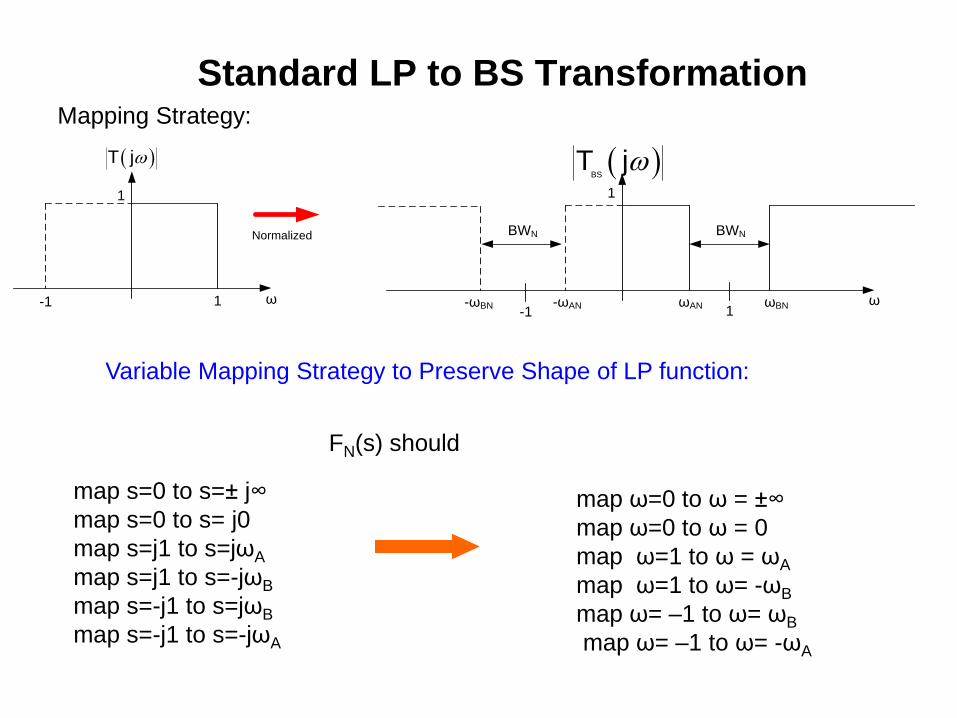
Standard LP to BS TransformationMapping Strategy:
map s=0 to s=± j∞
map s=0 to s= j0
map s=j1 to s=jωA
map s=j1 to s=-jωB
map s=-j1 to s=jωB
map s=-j1 to s=-jωA
FN(s) should
map ω=0 to ω = ±∞
map ω=0 to ω = 0
map ω=1 to ω = ωA
map ω=1 to ω= -ωB
map ω= –1 to ω= ωB
map ω= –1 to ω= -ωA
Variable Mapping Strategy to Preserve Shape of LP function:
1
1
ω1
1
ω
T j BS
T j
Normalized
-1-1
BWNBWN
ωBN-ωBN ωAN-ωAN
ω
1
1
ω
1
T j
BS
T j
-1
ω = ∞ω = - ∞
ω0-ω0 1-1
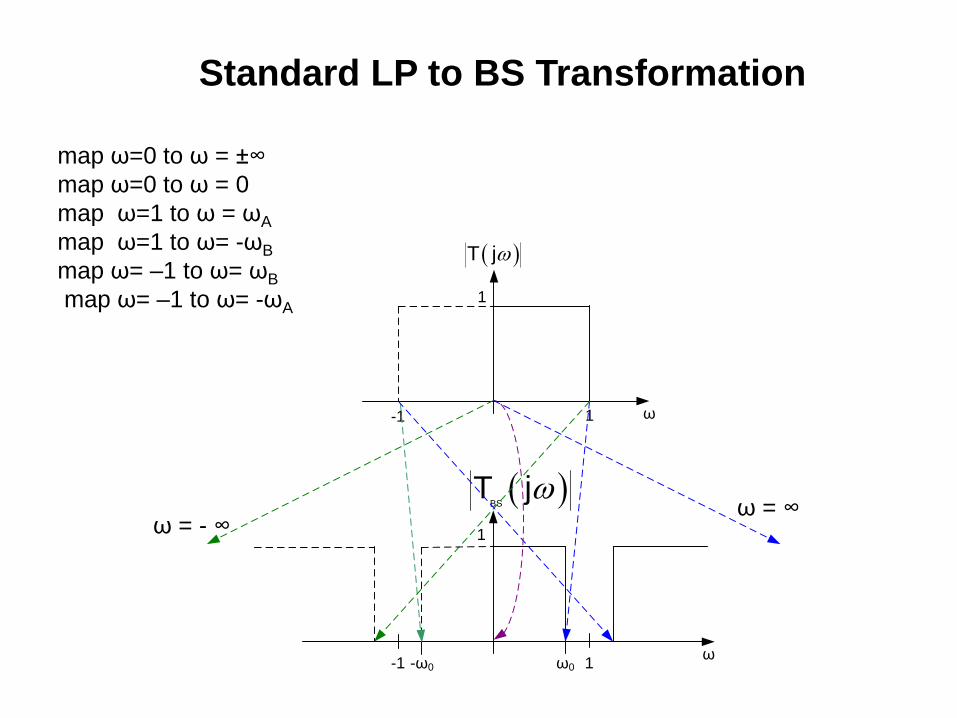
Standard LP to BS Transformation
map ω=0 to ω = ±∞
map ω=0 to ω = 0
map ω=1 to ω = ωA
map ω=1 to ω= -ωB
map ω= –1 to ω= ωB
map ω= –1 to ω= -ωA
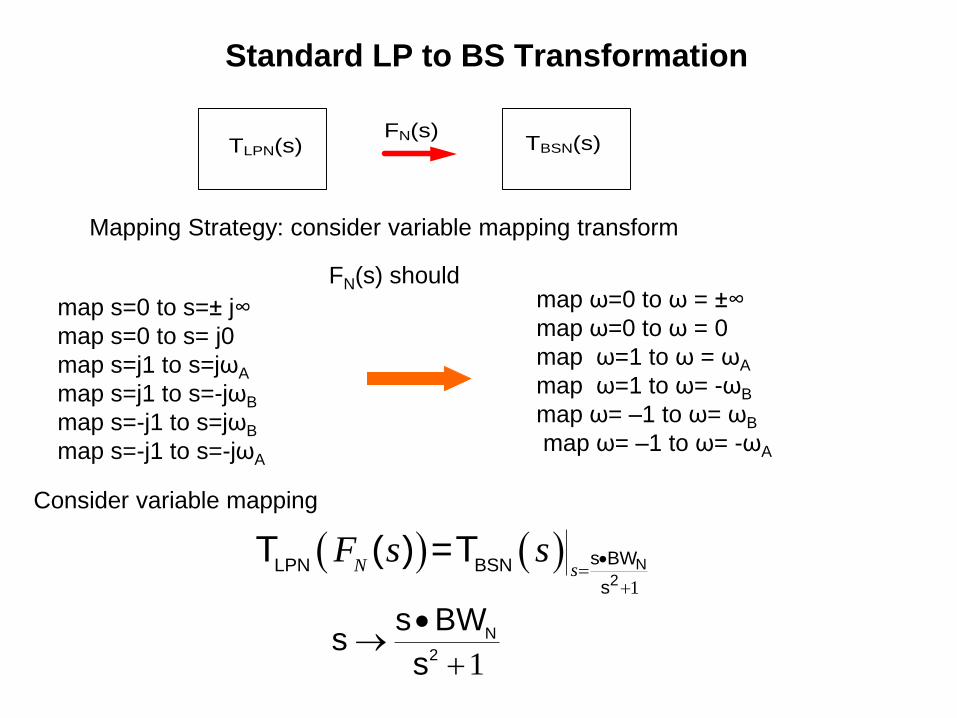
Standard LP to BS Transformation
Mapping Strategy: consider variable mapping transform
TLPN(s) TBSN(s)FN(s)
FN(s) should
Consider variable mapping
1
N2
s BWLPN BSN
s
T ( ) =TN s
F s s
1N
2
s BWs
s
map s=0 to s=± j∞
map s=0 to s= j0
map s=j1 to s=jωA
map s=j1 to s=-jωB
map s=-j1 to s=jωB
map s=-j1 to s=-jωA
map ω=0 to ω = ±∞
map ω=0 to ω = 0
map ω=1 to ω = ωA
map ω=1 to ω= -ωB
map ω= –1 to ω= ωB
map ω= –1 to ω= -ωA
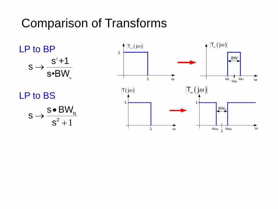
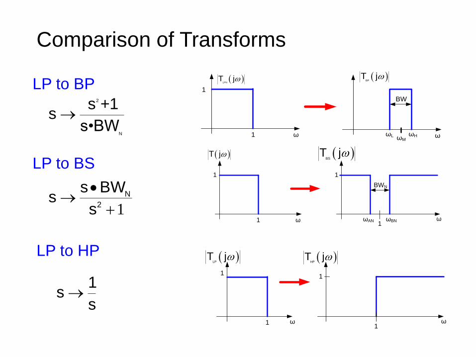
Comparison of Transforms
1N
2
s BWs
s
2
N
s +1s
s•BW
LP to BP
LP to BS
1
1
ω1
1
ω
T j BS
T j
BWN
ωBNωAN
ω
LPN
T j
ω
BP
T j
1
1
ωM
BW
ωL ωH
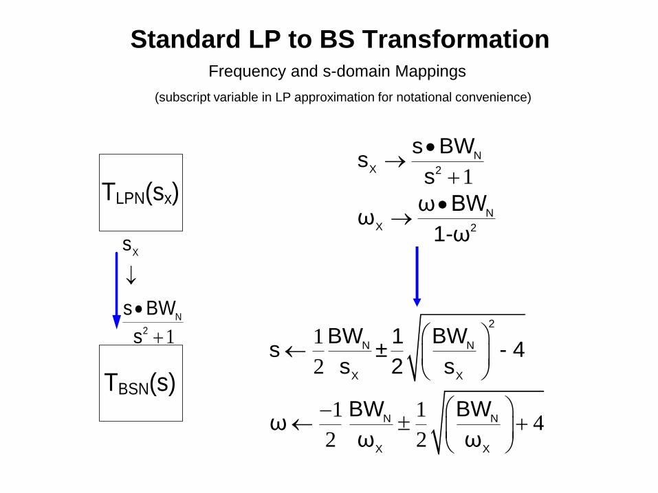
Standard LP to BS TransformationFrequency and s-domain Mappings
(subscript variable in LP approximation for notational convenience)
TLPN(sx)
TBSN(s)
1
X
N
2
s
s BW
s
1N
X 2
s BWs
s
N
X 2
ω BWω
1-ω
1
2
2
N N
X X
BW BW1s ± - 4
s 2 s
1 14
2 2N N
X X
BW BWω
ω ω
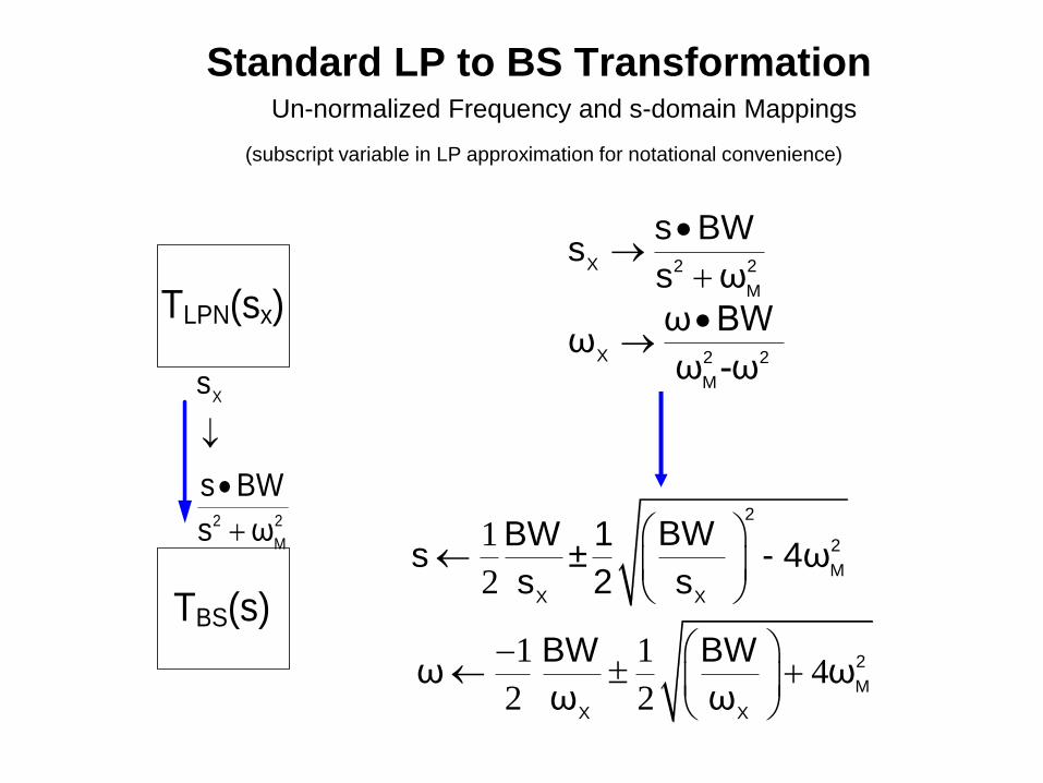
Standard LP to BS TransformationUn-normalized Frequency and s-domain Mappings
(subscript variable in LP approximation for notational convenience)
TLPN(sx)
TBS(s)
X
2 2
M
s
s BW
s ω
X 2 2
M
s BWs
s ω
X 2 2
M
ω BWω
ω -ω
1
2
2
2
M
X X
BWBW 1s ± - 4ω
s 2 s
1 14
2 2
2
M
X X
BW BWω ω
ω ω
Standard LP to BS TransformationPole Mappings
Can show that the upper hp pole maps to one upper hp pole and one lower hp pole
as shown. Corresponding mapping of the lower hp pole is also shown
Re
Im
Re
Im
0BPH LBPHω ,Q
0LPN LPω ,Q
0BPL LBPLω ,Q
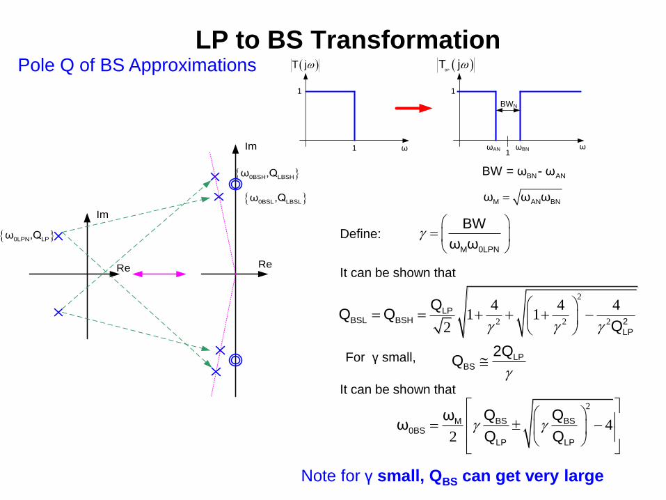
LP to BS TransformationPole Q of BS Approximations
Define:M 0LPN
BW
ω ω
BN ANBW = ω - ω
M AN BNω ω ω
It can be shown that
2
2 2 2
4 4 41 1
2
LPBSL BSH 2
LP
QQ Q
Q
For γ small, LPBS
2QQ
It can be shown that 2
42
BS BSM0BS
LP LP
Q Qωω
Q Q
Note for γ small, QBS can get very large
Re
Im
Re
Im
0BSH LBSHω ,Q
0LPN LPω ,Q
0BSL LBSLω ,Q
1
1
ω1
1
ω
T j BP
T j
BWN
ωBNωAN
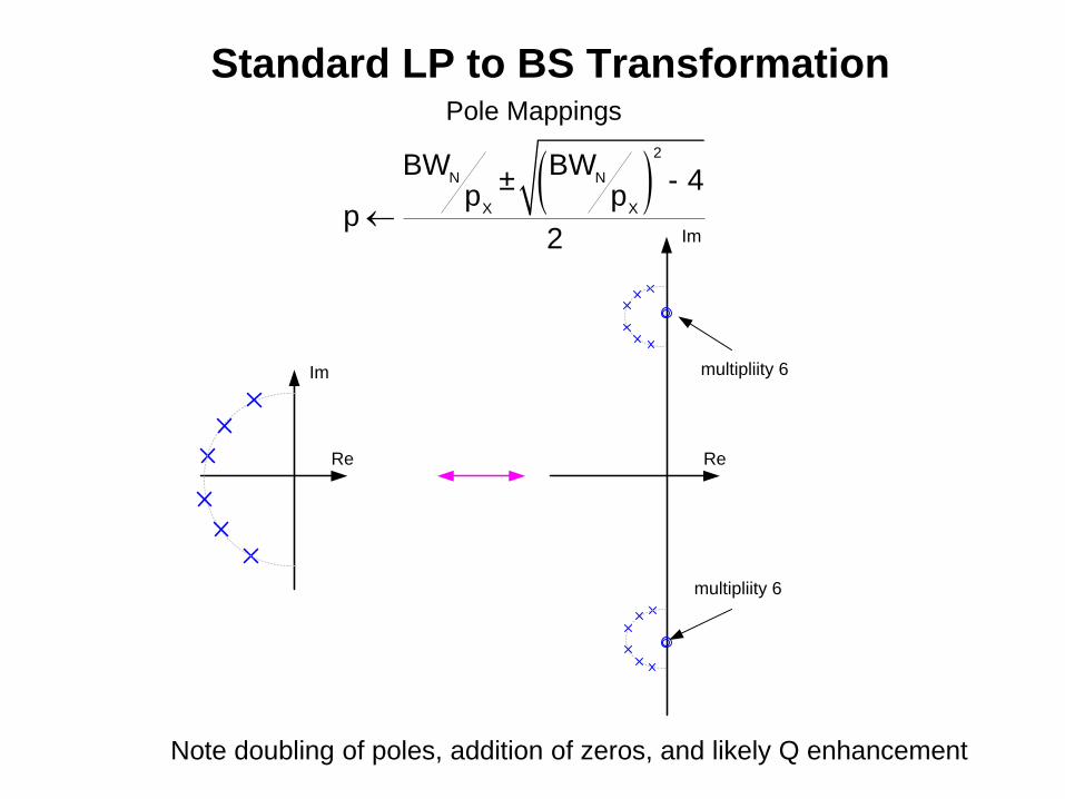
Standard LP to BS TransformationPole Mappings
2
N N
X X
BW BW± - 4
p pp
2
Note doubling of poles, addition of zeros, and likely Q enhancement
Re
Im
Re
Im
multipliity 6
multipliity 6
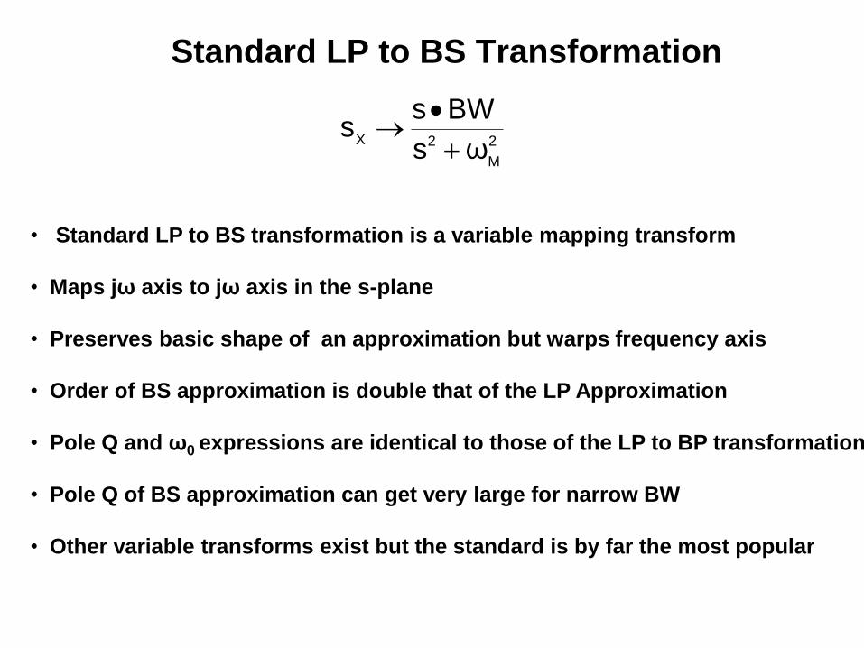
Standard LP to BS Transformation
• Standard LP to BS transformation is a variable mapping transform
• Maps jω axis to jω axis in the s-plane
• Preserves basic shape of an approximation but warps frequency axis
• Order of BS approximation is double that of the LP Approximation
• Pole Q and ω0 expressions are identical to those of the LP to BP transformation
• Pole Q of BS approximation can get very large for narrow BW
• Other variable transforms exist but the standard is by far the most popular
X 2 2
M
s BWs
s ω
Filter Transformations
Lowpass to Bandpass (LP to BP)
Lowpass to Highpass (LP to HP)
Lowpass to Band-reject (LP to BR)
• Approach will be to take advantage of the results obtained for the
standard LP approximations
• Will focus on flat passband and zero-gain stop-band
transformations
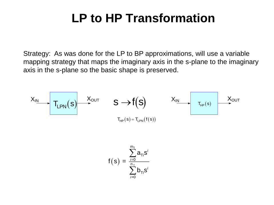
LP to HP Transformation
Strategy: As was done for the LP to BP approximations, will use a variable
mapping strategy that maps the imaginary axis in the s-plane to the imaginary
axis in the s-plane so the basic shape is preserved.
XIN XOUT
LPNT sXIN XOUT
HPT s s f s
HP LPNT s T f s
T
T
m
Ti
=0
n
Ti
=0
a s
f s =
b s
i
i
i
i
1
1
ω1
1
ω
T j HP
T j
Normalized
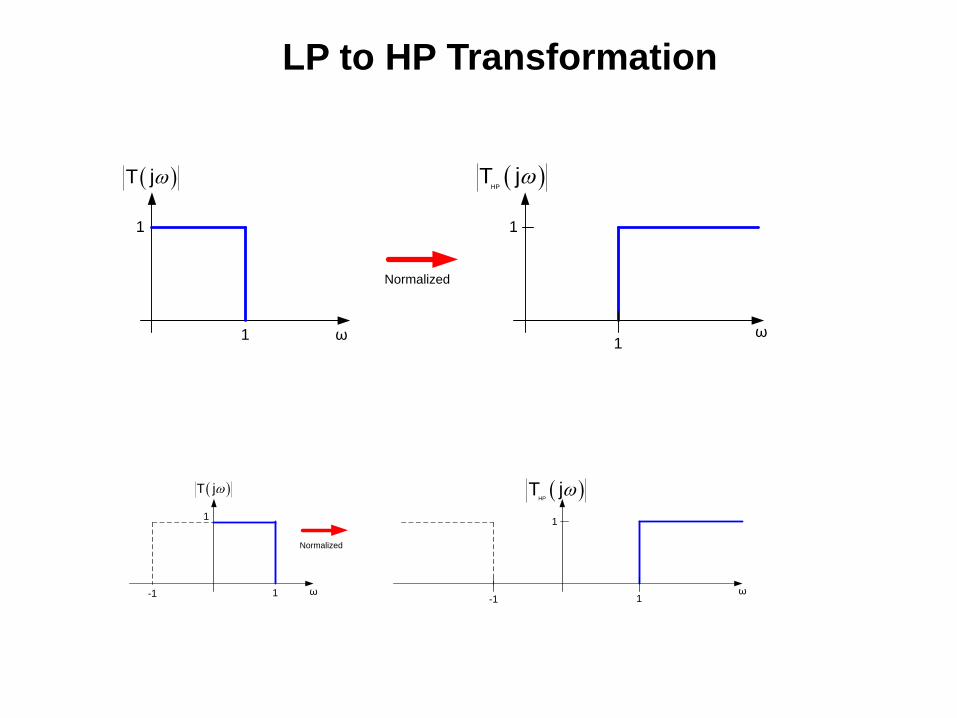
LP to HP Transformation
1
1
ω1
1
ω
T j HP
T j
Normalized
-1-1
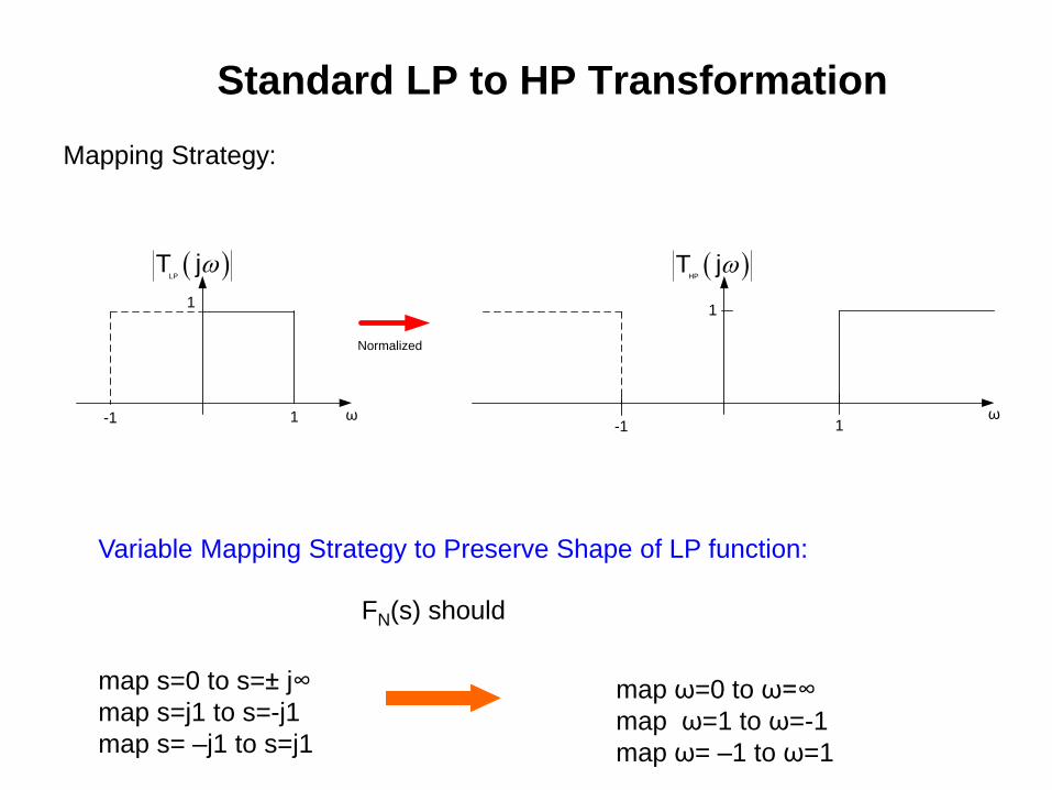
Standard LP to HP Transformation
Mapping Strategy:
map s=0 to s=± j∞
map s=j1 to s=-j1
map s= –j1 to s=j1
FN(s) should
map ω=0 to ω=∞
map ω=1 to ω=-1
map ω= –1 to ω=1
Variable Mapping Strategy to Preserve Shape of LP function:
1
1
ω1
1
ω
LP
T j HP
T j
Normalized
-1-1
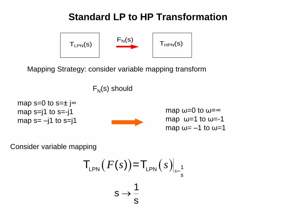
Standard LP to HP Transformation
Mapping Strategy: consider variable mapping transform
TLPN(s) THPN(s)FN(s)
FN(s) should
Consider variable mapping
1LPN LPNs
T ( ) =Ts
F s s
1s
s
map s=0 to s=± j∞
map s=j1 to s=-j1
map s= –j1 to s=j1
map ω=0 to ω=∞
map ω=1 to ω=-1
map ω= –1 to ω=1
Comparison of Transforms
1N
2
s BWs
s
2
N
s +1s
s•BW
LP to BP
LP to BS
1
1
ω1
1
ω
T j BS
T j
BWN
ωBNωAN
ω
LPN
T j
ω
BP
T j
1
1
ωM
BW
ωL ωH
LP to HP
1s
s
1
1
ω1
1
ω
LP
T j HP
T j
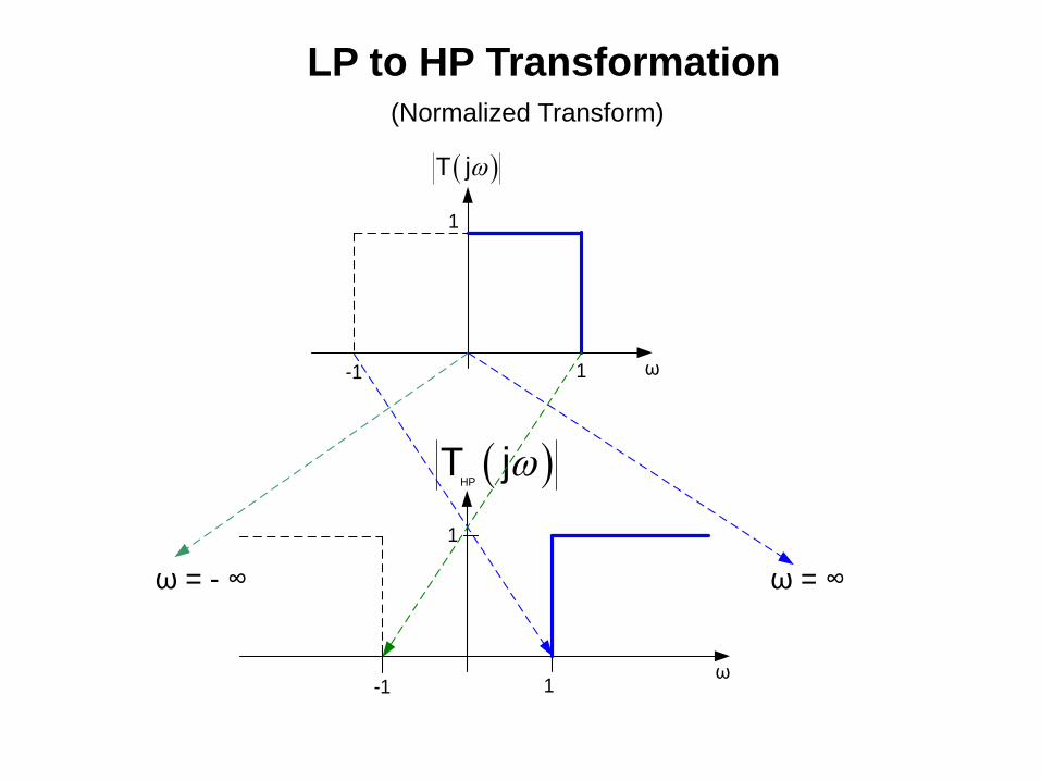
LP to HP Transformation
ω
1
1
ω
1
1
T j
HP
T j
-1
-1
ω = ∞ω = - ∞
(Normalized Transform)
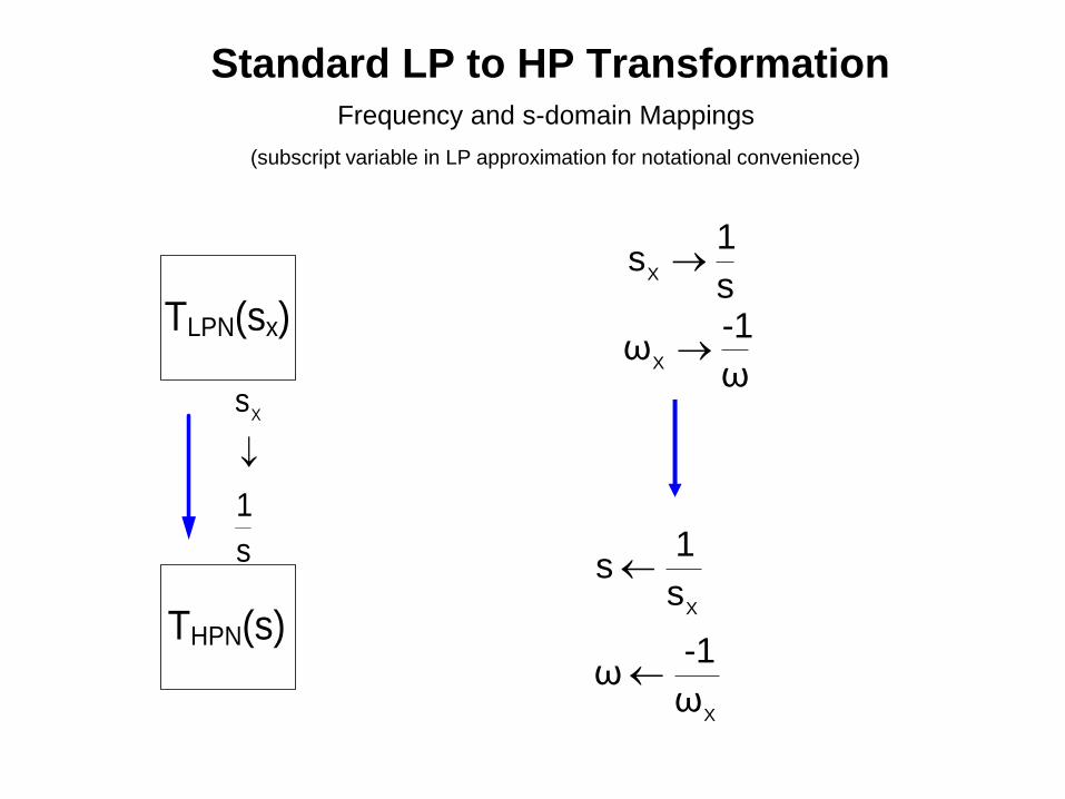
Standard LP to HP TransformationFrequency and s-domain Mappings
(subscript variable in LP approximation for notational convenience)
TLPN(sx)
THPN(s)
Xs
1
s
X
1s
s
X
-1ω
ω
X
1s
s
X
-1ω
ω
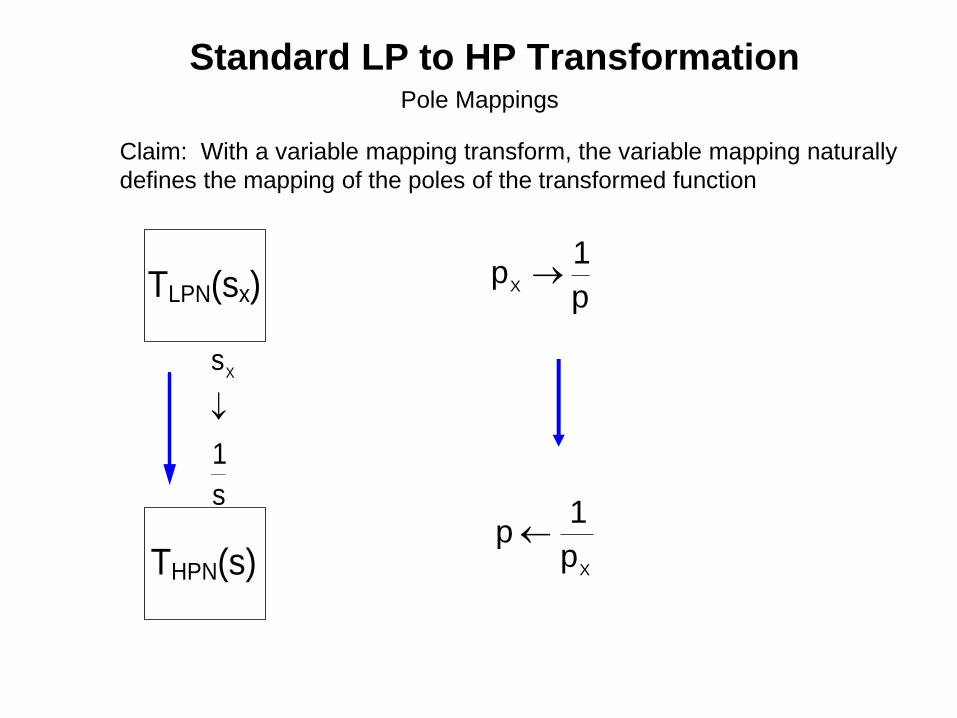
Standard LP to HP TransformationPole Mappings
TLPN(sx)
THPN(s)
Xs
1
s
X
1p
p
X
1p
p
Claim: With a variable mapping transform, the variable mapping naturally
defines the mapping of the poles of the transformed function
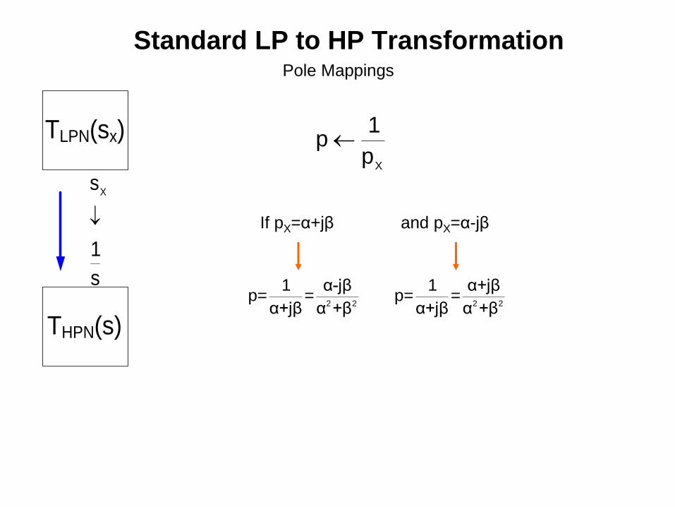
Standard LP to HP TransformationPole Mappings
TLPN(sx)
THPN(s)
Xs
1
s
X
1p
p
If pX=α+jβ
2 2
1 α-jβp= =
α+jβ α +β
and pX=α-jβ
2 2
1 α+jβp= =
α+jβ α +β
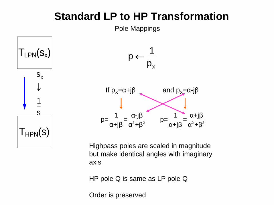
Standard LP to HP TransformationPole Mappings
TLPN(sx)
THPN(s)
Xs
1
s
X
1p
p
If pX=α+jβ
2 2
1 α-jβp= =
α+jβ α +β
and pX=α-jβ
2 2
1 α+jβp= =
α+jβ α +β
Highpass poles are scaled in magnitude
but make identical angles with imaginary
axis
HP pole Q is same as LP pole Q
Order is preserved
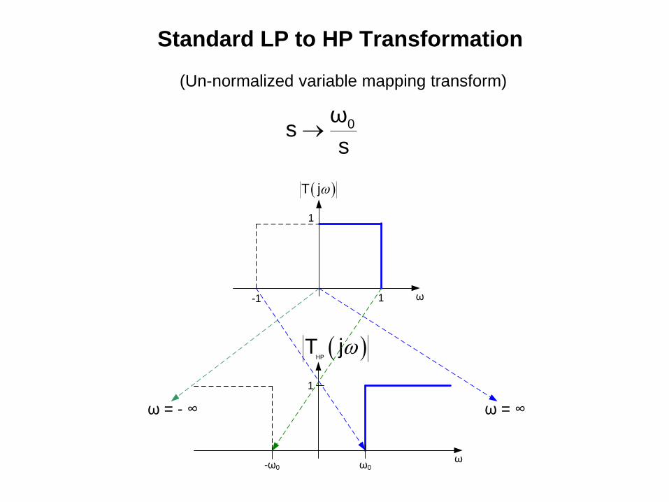
Standard LP to HP Transformation
0ωs
s
(Un-normalized variable mapping transform)
ω
1
1
ω
1
T j
HP
T j
-1
ω = ∞ω = - ∞
ω0-ω0
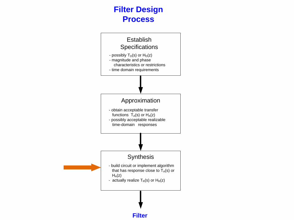
Filter Design
Process
Establish
Specifications
- possibly TD(s) or HD(z)
- magnitude and phase
characteristics or restrictions
- time domain requirements
Approximation
- obtain acceptable transfer
functions TA(s) or HA(z)
- possibly acceptable realizable
time-domain responses
Synthesis
- build circuit or implement algorithm
that has response close to TA(s) or
HA(z)
- actually realize TR(s) or HR(z)
Filter

End of Lecture 16