EE 4990/6990AntennasFall 2002

Page Lecture Material from Balanis Problems

1 Ch. 1, Introduction, antenna types 2 Radiation, Ch. 2, Antenna patterns 2.2 3 Average power, radiation intensity 2.4, 2.7 4 Directivity, numerical evaluation of directivity 2.4, 2.7 5 Antenna gain 2.11, 2.13, 6 Antenna efficiency and impedance 2.17(a), 2.21 7 Loss resistance, transmission lines 2.27, 2.39 8 Transmit/receive systems, Polarization 2.41, 2.46 9 Equivalent areas, effective aperture 2.29, 2.4810 Friis transmission equation 2.53, 2.56, 2.5811 Radar systems, radar cross section 2.62, 2.6612 Problem Session13 Quiz #1 [Ch. 1,2]14 Ch. 3, Radiated fields15 Use of potential functions16 Far fields, duality, reciprocity 4.185 Ch. 4, Wire antennas, infinitesimal dipole 4.318 Infinitesimal dipole 4.519 Poynting’s theorem, total power 4.11, 4.1520 Radiation resistance, Short dipole 4.18(b), 4.2121 Center-fed dipole 4.31123 Half-wave dipole 4.25, 4.2623 Dipole characteristics 4.27, 4.3324 Image theory, antennas over ground 4.3725 Monopole 4.41, 4.4426 Ground Effects on Antennas27 Quiz #2 [Ch. 3,4] 28 Ch. 5, Small loop antenna 5.4 29 Dual sources 5.1730 Loop characteristics 5.21162 Ch. 6, Antenna arrays 6.332 Broadside arrays 6.633 Endfire arrays 6.1634 Hansen-Woodyard array, Binomial arrays 6.24, 6.2835 Dolph-Chebyshev array, 6.41191 Ch. 9, folded dipole 9.8, 9.10, 9.1237 Ch. 10, Traveling wave antennas 10.4, 10.638 Terminations, vee antenna, 10.2839 rhombic antenna, Yagi-Uda arrays 10.2840 Ch. 11, Log-periodic antenna 11.841 Problem Session 42 Quiz #3 [Ch. 5,6,9,10,11] 43 Ch. 12, Aperture antennas44 Ch. 13, Horn antennas 13.7, 13.1245 Course review

Antennas

Antenna - a device used to efficiently transmit and/or receiveelectromagnetic waves.

Example Antenna Applications

Wireless communicationsPersonal Communications Systems (PCS)Global Positioning Satellite (GPS) SystemsWireless Local Area Networks (WLAN)Direct Broadcast Satellite (DBS) TelevisionMobile CommunicationsTelephone Microwave/Satellite LinksBroadcast Television and Radio, etc.

Remote SensingRadar [active remote sensing - radiate and receive]

Military applications (target search and tracking)Weather radar, Air traffic controlAutomobile speed detectionTraffic control (magnetometer)Ground penetrating radar (GPR)Agricultural applications

Radiometry [passive remote sensing - receive emissions]Military applications

(threat avoidance, signal interception)

Antenna Types

Wire antennas (monopoles, dipoles, loops, etc.)Aperture antennas (sectoral horn, pyramidal horn, slots, etc.)Reflector antennas (parabolic dish, corner reflector, etc.)Lens antennasMicrostrip antennasAntenna arrays

Antenna Performance Parameters

Radiation pattern - angular plot of the radiation.Omnidirectional pattern - uniform radiation in one planeDirective patterns - narrow beam(s) of high radiation

Directivity - ratio of antenna power density at a distant point relativeto that of an isotropic radiator [isotropic radiator - an antennathat radiates uniformly in all directions (point source radiator)].

Gain - directivity reduced by losses.

Polarization - trace of the radiated electric field vector (linear,circular, elliptical).

Impedance - antenna input impedance at its terminals.

Bandwidth - range of frequencies over which performance isacceptable (resonant antennas, broadband antennas).

Beam scanning - movement in the direction of maximum radiationby mechanical or electrical means.

Other system design constraints - size, weight, cost, power handling,radar cross section, etc.

Fundamentals of Antenna Radiation

An antenna may be thought of as a matching network between awave-guiding device (transmission line, waveguide) and the surroundingmedium.

Transmitting antenna

guided wave input antenna unguided wave output

Receiving antenna

unguided wave input antenna guided wave output

Antenna as the termination of a transmission line

The open-circuited transmission line does not radiate effectively becausethe transmission line currents are equal and opposite (and very closetogether). The radiated fields of these currents tend to cancel one another.The current on the arms of the dipole antenna are aligned in the samedirection so that these radiated fields tend to add together making thedipole and efficient radiator.

Antenna as the termination of a waveguide

The open-ended waveguide will radiate, but not as effectively as thewaveguide terminated by the horn antenna. The wave impedance insidethe waveguide does not match that of the surrounding medium creating amismatch at the open end of the waveguide. Thus, a portion of theoutgoing wave is reflected back into the waveguide. The horn antenna actsas a matching network, with a gradual transition in the wave impedancefrom that of the waveguide to that of the surrounding medium. With amatched termination, the reflected wave is minimized and the radiatedfield is maximized.

Antenna Patterns(Radiation Patterns)

Antenna Pattern - a graphical representation of the antenna radiationproperties as a function of position (spherical coordinates).

Common Types of Antenna Patterns

Power Pattern - normalized power vs. spherical coordinate position.

Field Pattern - normalized E or H vs. spherical coordinateposition.

Antenna Field Types

Reactive field - the portion of the antenna field characterized bystanding (stationary) waves which represent stored energy.

Radiation field - the portion of the antenna field characterized byradiating (propagating) waves which represent transmittedenergy.

Antenna Field Regions

Reactive Near Field Region - the region immediately surroundingthe antenna where the reactive field (stored energy - standingwaves) is dominant.

Near-Field (Fresnel) Region - the region between the reactive near-field and the far-field where the radiation fields are dominantand the field distribution is dependent on the distance from theantenna.

Far-Field (Fraunhofer) Region - the region farthest away from theantenna where the field distribution is essentially independentof the distance from the antenna (propagating waves).

Antenna Field Regions

Antenna Pattern Definitions

Isotropic Pattern - an antenna pattern defined by uniform radiationin all directions, produced by an isotropic radiator (pointsource, a non-physical antenna which is the only nondirectionalantenna).

Directional Pattern - a pattern characterized by more efficientradiation in one direction than another (all physically realizableantennas are directional antennas).

Omnidirectional Pattern - a pattern which is uniform in a givenplane.

Principal Plane Patterns - the E-plane and H-plane patterns of alinearly polarized antenna.

E-plane - the plane containing the electric field vectorand the direction of maximum radiation.

H-plane - the plane containing the magnetic field vectorand the direction of maximum radiation.

Antenna Pattern Parameters

Radiation Lobe - a clear peak in the radiation intensity surroundedby regions of weaker radiation intensity.

Main Lobe (major lobe, main beam) - radiation lobe in the directionof maximum radiation.

Minor Lobe - any radiation lobe other than the main lobe.

Side Lobe - a radiation lobe in any direction other than thedirection(s) of intended radiation.

Back Lobe - the radiation lobe opposite to the main lobe.

Half-Power Beamwidth (HPBW) - the angular width of the mainbeam at the half-power points.

First Null Beamwidth (FNBW) - angular width between the firstnulls on either side of the main beam.

Antenna Pattern Parameters(Normalized Power Pattern)

Maxwell’s Equations(Instantaneous and Phasor Forms)

Maxwell’s Equations (instantaneous form)

- instantaneous vectors [ = (x,y,z,t), etc.]t - instantaneous scalar

Maxwell’s Equations (phasor form, time-harmonic form)

E, H, D, B, J - phasor vectors [E=E(x,y,z), etc.] - phasor scalar

Relation of instantaneous quantities to phasor quantities ...

(x,y,z,t) = ReE(x,y,z)ejt, etc.

S

S S

s

ds

Average Power Radiated by an Antenna

To determine the average power radiated by an antenna, we start withthe instantaneous Poynting vector (vector power density) defined by

(V/m × A/m = W/m2)

Assume the antenna is enclosed by some surface S.

The total instantaneous radiated power rad leaving the surface S is foundby integrating the instantaneous Poynting vector over the surface.

radds = ()ds ds = s ds

ds = differential surface s = unit vector normal to ds

T

T

S

For time-harmonic fields, the time average instantaneous Poyntingvector (time average vector power density) is found by integrating theinstantaneous Poynting vector over one period (T) and dividing by theperiod. 1

Pavg = () dt T

= ReEejt

= ReHejt

The instantaneous magnetic field may be rewritten as

= Re½ [ Hejt + H*ejt ]

which gives an instantaneous Poynting vector of

½ Re [E H]ej2t + [E H*] ~~~~~~~~~~~~~~~ ~~~~~~~ time-harmonic independent of time (integrates to zero over T )

and the time-average vector power density becomes 1

Pavg = Re [E H*] dt 2T

= ½ Re [E H*]

The total time-average power radiated by the antenna (Prad) is found byintegrating the time-average power density over S.

PradPavgds = ½ Re [E H*]ds S

S

Radiation Intensity

Radiation Intensity - radiated power per solid angle (radiated powernormalized to a unit sphere).

PradPavgds

In the far field, the radiation electric and magnetic fields vary as 1/r andthe direction of the vector power density (Pavg) is radially outward. If weassume that the surface S is a sphere of radius r, then the integral for thetotal time-average radiated power becomes

If we defined Pavgr2 = U(,) as the radiation intensity, then

where d = sindd defines the differential solid angle. The units on theradiation intensity are defined as watts per unit solid angle. The averageradiation intensity is found by dividing the radiation intensity by the areaof the unit sphere (4) which gives

The average radiation intensity for a given antenna represents the radiationintensity of a point source producing the same amount of radiated poweras the antenna.

19

RadianRadian

Fig. 2.10(a) Geometrical arrangements for defining a radian

r

2 radians in full circle

arc length of circle

20

SteradianSteradian

one steradian subtends an area of

4 steradians in entire sphere

ddrdA sin2

Fig. 2.10(b) Geometrical arrangements

for defining a steradian.

ddr

dAd sin

2

2rA

21

Radiation power densityRadiation power density

HEW

Instantaneous

Poynting vector

Time average

Poynting vector

[ W/m ² ]

Total instantaneous

PowerAverage radiated

Power

[ W/m ² ]

s

sWP d [ W ]

HEW Re2

1avg

s

avgrad dP sW

[ W ]

[2-8]

[2-9]

[2-4]

[2-3]

22

Radiation intensityRadiation intensity

“Power radiated per unit solid angle”

avgWrU 2

far zone fields without 1/r factor

22

),,(2

),( rr

U E

222

),,(),,(2

rErEr

[W/unit solid angle]

[2-12a]

Directivity

Directivity (D) - the ratio of the radiation intensity in a given directionfrom the antenna to the radiation intensity averaged over alldirections.

The directivity of an isotropic radiator is D(,) = 1.

The maximum directivity is defined as [D(,)]max = Do.

The directivity range for any antenna is 0 D(,) Do.

Directivity in dB

Directivity in terms of Beam Solid Angle

We may define the radiation intensity as

where Bo is a constant and F(,) is the radiation intensity patternfunction. The directivity then becomes

and the radiated power is

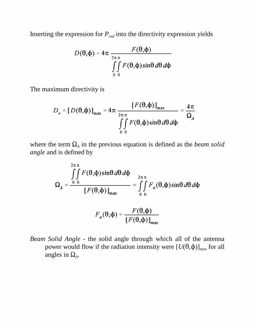
Inserting the expression for Prad into the directivity expression yields

The maximum directivity is

where the term A in the previous equation is defined as the beam solidangle and is defined by

Beam Solid Angle - the solid angle through which all of the antennapower would flow if the radiation intensity were [U(,)]max for allangles in A.

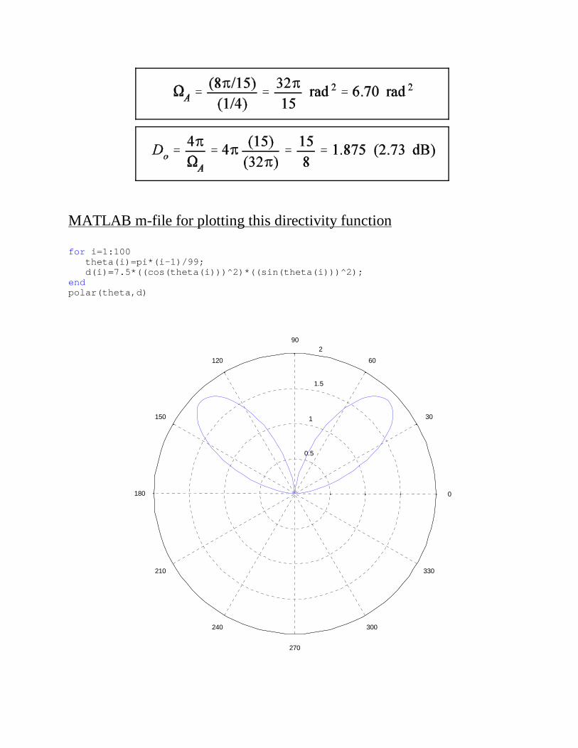
Example (Directivity/Beam Solid Angle/Maximum Directivity)

Determine the directivity [D(,)], the beam solid angle A and themaximum directivity [Do] of an antenna defined by F(,) =sin2cos2.

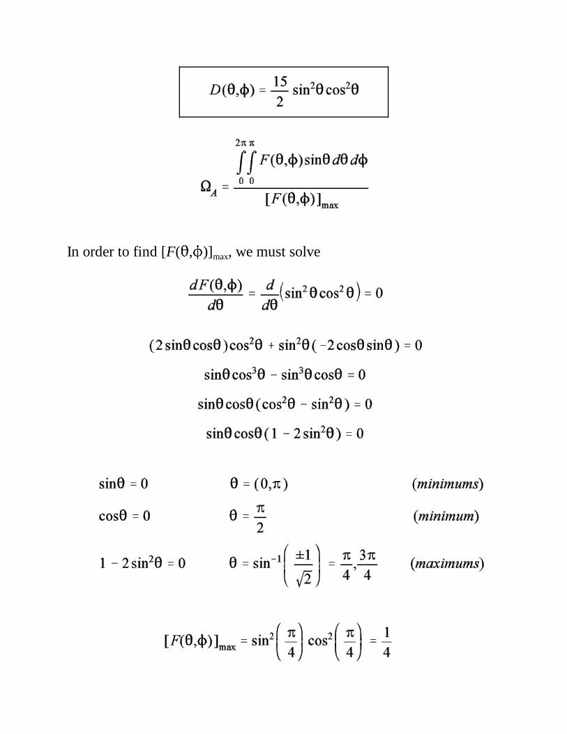
In order to find [F(,)]max, we must solve

0.5

1

1.5

2

30

210

60

240

90

270

120

300

150

330

180 0

MATLAB m-file for plotting this directivity function

for i=1:100 theta(i)=pi*(i-1)/99; d(i)=7.5*((cos(theta(i)))^2)*((sin(theta(i)))^2);endpolar(theta,d)

Directivity/Beam Solid Angle Approximations

Given an antenna with one narrow major lobe and negligible radiationin its minor lobes, the beam solid angle may be approximated by

where 1 and 2 are the half-power beamwidths (in radians) which areperpendicular to each other. The maximum directivity, in this case, isapproximated by

If the beamwidths are measured in degrees, we have

Example (Approximate Directivity)

A horn antenna with low side lobes has half-power beamwidths of29o in both principal planes (E-plane and H-plane). Determine theapproximate directivity (dB) of the horn antenna.

Numerical Evaluation of Directivity

The maximum directivity of a given antenna may be written as

where U() = BoF(,). The integrals related to the radiated power inthe denominators of the terms above may not be analytically integrable. In this case, the integrals must be evaluated using numerical techniques.If we assume that the dependence of the radiation intensity on and isseparable, then we may write

The radiated power integral then becomes

Note that the assumption of a separable radiation intensity pattern functionresults in the product of two separate integrals for the radiated power. Wemay employ a variety of numerical integration techniques to evaluate theintegrals. The most straightforward of these techniques is the rectangularrule (others include the trapezoidal rule, Gaussian quadrature, etc.) If wefirst consider the -dependent integral, the range of is first subdividedinto N equal intervals of length

The known function f () is then evaluated at the center of eachsubinterval. The center of each subinterval is defined by

The area of each rectangular sub-region is given by

The overall integral is then approximated by

Using the same technique on the -dependent integral yields

Combining the and dependent integration results gives theapproximate radiated power.

The approximate radiated power for antennas that are omnidirectional withrespect to [g() = 1] reduces to

The approximate radiated power for antennas that are omnidirectional withrespect to [ f() = 1] reduces to

For antennas which have a radiation intensity which is not separable in and , the a two-dimensional numerical integration must be performedwhich yields

Example (Numerical evaluation of directivity)

Determine the directivity of a half-wave dipole given the radiationintensity of

The maximum value of the radiation intensity for a half-wave dipoleoccurs at = /2 so that

MATLAB m-file

sum=0.0;N=input(’Enter the number of segments in the theta direction’)for i=1:N thetai=(pi/N)*(i-0.5); sum=sum+(cos((pi/2)*cos(thetai)))^2/sin(thetai);endD=(2*N)/(pi*sum)

N Do

5 1.6428

10 1.6410

15 1.6409

20 1.6409

Antenna Efficiency

When an antenna is driven by a voltage source (generator), the totalpower radiated by the antenna will not be the total power available fromthe generator. The loss factors which affect the antenna efficiency can beidentified by considering the common example of a generator connectedto a transmitting antenna via a transmission line as shown below.

Zg - source impedance

ZA - antenna impedance

Zo - transmission line characteristic impedance

Pin - total power delivered to the antenna terminals

Pohmic - antenna ohmic (I2R) losses [conduction loss + dielectric loss]

Prad - total power radiated by the antenna

The total power delivered to the antenna terminals is less than thatavailable from the generator given the effects of mismatch at the source/t-line connection, losses in the t-line, and mismatch at the t-line/antennaconnection. The total power delivered to the antenna terminals must equalthat lost to I2R (ohmic) losses plus that radiated by the antenna.

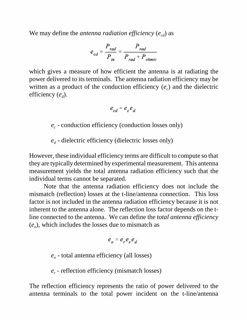
We may define the antenna radiation efficiency (ecd) as

which gives a measure of how efficient the antenna is at radiating thepower delivered to its terminals. The antenna radiation efficiency may bewritten as a product of the conduction efficiency (ec) and the dielectricefficiency (ed).

ec - conduction efficiency (conduction losses only)

ed - dielectric efficiency (dielectric losses only)

However, these individual efficiency terms are difficult to compute so thatthey are typically determined by experimental measurement. This antennameasurement yields the total antenna radiation efficiency such that theindividual terms cannot be separated.

Note that the antenna radiation efficiency does not include themismatch (reflection) losses at the t-line/antenna connection. This lossfactor is not included in the antenna radiation efficiency because it is notinherent to the antenna alone. The reflection loss factor depends on the t-line connected to the antenna. We can define the total antenna efficiency(eo), which includes the losses due to mismatch as

eo - total antenna efficiency (all losses)

er - reflection efficiency (mismatch losses)

The reflection efficiency represents the ratio of power delivered to theantenna terminals to the total power incident on the t-line/antenna

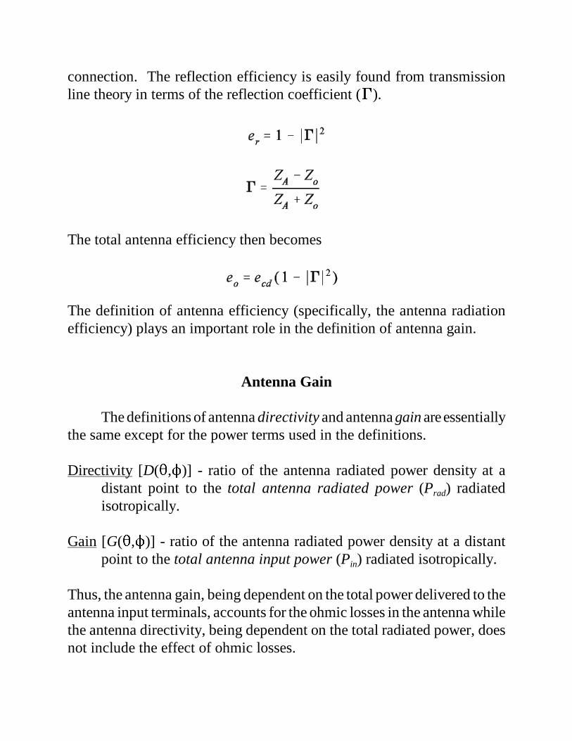
connection. The reflection efficiency is easily found from transmissionline theory in terms of the reflection coefficient ().

The total antenna efficiency then becomes

The definition of antenna efficiency (specifically, the antenna radiationefficiency) plays an important role in the definition of antenna gain.

Antenna Gain

The definitions of antenna directivity and antenna gain are essentiallythe same except for the power terms used in the definitions.

Directivity [D(,)] - ratio of the antenna radiated power density at adistant point to the total antenna radiated power (Prad) radiatedisotropically.

Gain [G(,)] - ratio of the antenna radiated power density at a distantpoint to the total antenna input power (Pin) radiated isotropically.

Thus, the antenna gain, being dependent on the total power delivered to theantenna input terminals, accounts for the ohmic losses in the antenna whilethe antenna directivity, being dependent on the total radiated power, doesnot include the effect of ohmic losses.

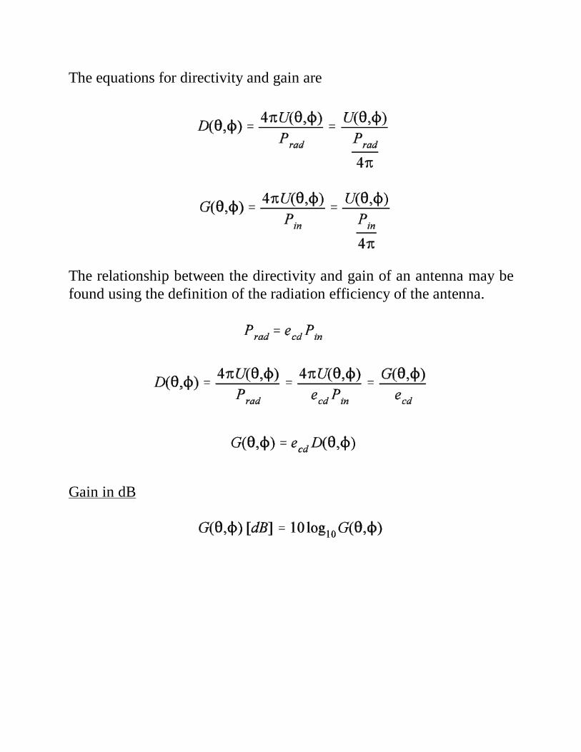
The equations for directivity and gain are

The relationship between the directivity and gain of an antenna may befound using the definition of the radiation efficiency of the antenna.

Gain in dB

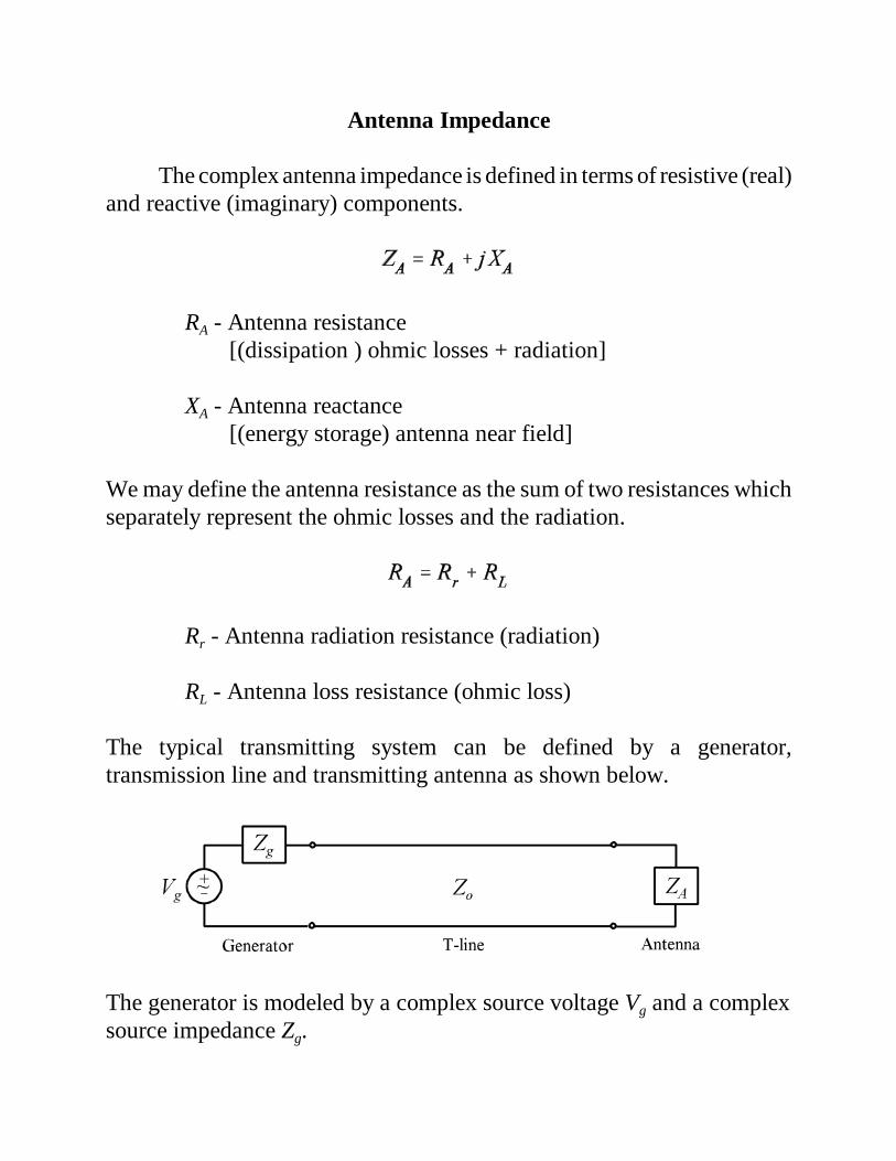
Antenna Impedance

The complex antenna impedance is defined in terms of resistive (real)and reactive (imaginary) components.

RA - Antenna resistance [(dissipation ) ohmic losses + radiation]

XA - Antenna reactance [(energy storage) antenna near field]

We may define the antenna resistance as the sum of two resistances whichseparately represent the ohmic losses and the radiation.

Rr - Antenna radiation resistance (radiation)

RL - Antenna loss resistance (ohmic loss)

The typical transmitting system can be defined by a generator,transmission line and transmitting antenna as shown below.

The generator is modeled by a complex source voltage Vg and a complexsource impedance Zg.

In some cases, the generator may be connected directly to the antenna.

Inserting the complete source and antenna impedances yields

The complex power associated with any element in the equivalent circuitis given by

where the * denotes the complex conjugate. We will assume peak valuesfor all voltages and currents in expressing the radiated power, the powerassociated with ohmic losses, and the reactive power in terms of specificcomponents of the antenna impedance. The peak current for the simpleseries circuit shown above is

The power radiated by the antenna (Pr) may be written as

The power dissipated as heat (PL) may be written

The reactive power (imaginary component of the complex power) storedin the antenna near field (PX) is

From the equivalent circuit for the generator/antenna system, we see thatmaximum power transfer occurs when

The circuit current in this case is

The power radiated by the antenna is

The power dissipated in heat is

The power available from the generator source is

Power dissipated in the generator [P/2]

Power available fromthe generator [P]

Power delivered to the antenna [P/2]

Power radiated by theantenna [ecd (P/2)]

Power dissipated by theantenna [(1ecd)(P/2)]

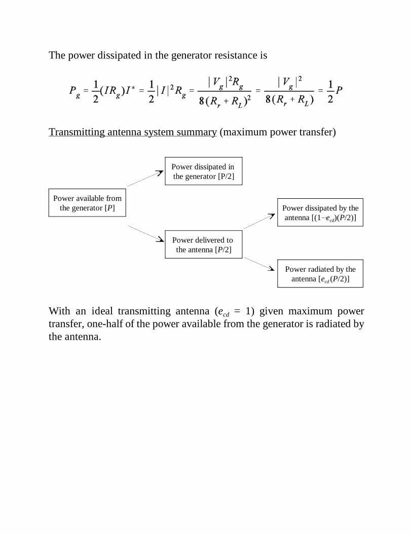
The power dissipated in the generator resistance is

Transmitting antenna system summary (maximum power transfer)

With an ideal transmitting antenna (ecd = 1) given maximum powertransfer, one-half of the power available from the generator is radiated bythe antenna.

The typical receiving system can be defined by a generator (receivingantenna), transmission line and load (receiver) as shown below.

Assuming the receiving antenna is connected directly to the receiver

For the receiving system, maximum power transfer occurs when

The circuit current in this case is

The power captured by the receiving antenna is

Some of the power captured by the receiving antenna is re-radiated(scattered). The power scattered by the antenna (Pscat) is

The power dissipated by the receiving antenna in the form of heat is

The power delivered to the receiver is

Power delivered to the receiver [P/2]

Power captured by the antenna [P]

Power delivered to the antenna [P/2]

Power scattered by theantenna [ecd (P/2)]

Power dissipated by theantenna [(1ecd)(P/2)]

Receiving antenna system summary (maximum power transfer)

With an ideal receiving antenna (ecd = 1) given maximum power transfer,one-half of the power captured by the antenna is re-radiated (scattered) bythe antenna.

Antenna Radiation Efficiency

The radiation efficiency (ecd) of a given antenna has previously beendefined in terms of the total power radiated by the antenna (Prad) and thetotal power dissipated by the antenna in the form of ohmic losses (Pohmic).

The total radiated power and the totalohmic losses were determined for thegeneral case of a transmitting antennausing the equivalent circuit. The totalradiated power is that “dissipated” inthe antenna radiation resistance (Rr).

The total ohmic losses for the antenna are those dissipated in the antennaloss resistance (RL).

Inserting the equivalent circuit results for Prad and Pohmic into the equationfor the antenna radiation efficiency yields

Thus, the antenna radiation efficiency may be found directly from theantenna equivalent circuit parameters.

Antenna Loss Resistance

The antenna loss resistance (conductor and dielectric losses) for manyantennas is typically difficult to calculate. In these cases, the lossresistance is normally measured experimentally. However, the lossresistance of wire antennas can be calculated easily and accurately.Assuming a conductor of length l and cross-sectional area A which carriesa uniform current density, the DC resistance is

where is the conductivity of the conductor. At high frequencies, thecurrent tends to crowd toward the outer surface of the conductor (skineffect). The HF resistance can be defined in terms of the skin depth .

where is the permeability of the material and f is the frequency in Hz.

The skin depth for copper ( = 5.8×107 /m, = o = 4×107 H/m) maybe written as

If we define the perimeter distance of the conductor as dp, then the HFresistance of the conductor can be written as

where Rs is defined as the surface resistance of the material.

For the RHF equation to be accurate, the skin depth should be a smallfraction of the conductor maximum cross-sectional dimension. In the caseof a cylindrical conductor (dp 2a), the HF resistance is

f R

0 RDC = 0.818 m

1 kHz 2.09 mm ~

10 kHz 0.661 mm RHF = 1.60 m

100 kHz 0.209 mm RHF = 5.07 m

1 MHz 0.0661mm

RHF = 16.0 m

Resistance of 1 m of #10 AWG (a = 2.59 mm) copper wire.

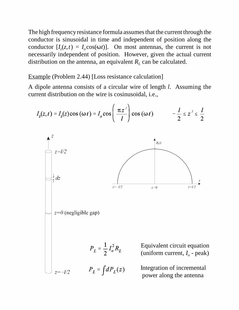
The high frequency resistance formula assumes that the current through theconductor is sinusoidal in time and independent of position along theconductor [Iz(z, t) = Iocos(t)]. On most antennas, the current is notnecessarily independent of position. However, given the actual currentdistribution on the antenna, an equivalent RL can be calculated.

Example (Problem 2.44) [Loss resistance calculation]

A dipole antenna consists of a circular wire of length l. Assuming thecurrent distribution on the wire is cosinusoidal, i.e.,

Equivalent circuit equation (uniform current, Io - peak)

Integration of incremental power along the antenna

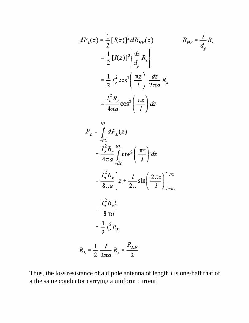
Thus, the loss resistance of a dipole antenna of length l is one-half that ofa the same conductor carrying a uniform current.

+z directedwaves

z directedwaves

Lossless Transmission Line Fundamentals

Transmission line equations (voltage and current)

~~~~~~~ ~~~~~~~

Transmitting/Receiving Systems with Transmission Lines

Using transmission line theory, the impedance seen looking intothe input terminals of the transmission line (Zin) is

The resulting equivalent circuit is shown below.

The current and voltage at the transmission line input terminals are

The power available from the generator is

The power delivered to the transmission line input terminals is

The power associated with the generator impedance is

Given the current and the voltage at the input to the transmission line, thevalues at any point on the line can be found using the transmission lineequations.

The unknown coefficient Vo+ may be determined from either V(0) or I(0)

which were found in the input equivalent circuit. Using V(0) gives

where

Given the coefficient Vo+, the current and voltage at the load, from the

transmission line equations are

The power delivered to the load is then

The complexity of the previous equations leads to solutions which aretypically determined by computer or Smith chart.

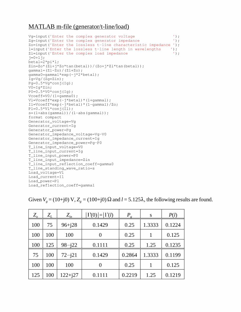
MATLAB m-file (generator/t-line/load)

Vg=input(’Enter the complex generator voltage ’);Zg=input(’Enter the complex generator impedance ’);Zo=input(’Enter the lossless t-line characteristic impedance ’);l=input(’Enter the lossless t-line length in wavelengths ’);Zl=input(’Enter the complex load impedance ’);j=0+1j;betal=2*pi*l;Zin=Zo*(Zl+j*Zo*tan(betal))/(Zo+j*Zl*tan(betal));gammal=(Zl-Zo)/(Zl+Zo);gamma0=gammal*exp(-j*2*betal);Ig=Vg/(Zg+Zin);Pg=0.5*Vg*conj(Ig);V0=Ig*Zin;P0=0.5*V0*conj(Ig);Vcoeff=V0/(1+gamma0);Vl=Vcoeff*exp(-j*betal)*(1+gammal);Il=Vcoeff*exp(-j*betal)*(1-gammal)/Zo;Pl=0.5*Vl*conj(Il);s=(1+abs(gammal))/(1-abs(gammal));format compactGenerator_voltage=VgGenerator_current=IgGenerator_power=PgGenerator_impedance_voltage=Vg-V0Generator_impedance_current=IgGenerator_impedance_power=Pg-P0T_line_input_voltage=V0T_line_input_current=IgT_line_input_power=P0T_line_input_impedance=ZinT_line_input_reflection_coeff=gamma0T_line_standing_wave_ratio=sLoad_voltage=VlLoad_current=IlLoad_power=PlLoad_reflection_coeff=gammal

Given Vg = (10+j0) V, Zg = (100+j0) and l = 5.125, the following results are found.

Zo ZL Zin (0)=(l) Pg s P(l)

100 75 96+j28 0.1429 0.25 1.3333 0.1224

100 100 100 0 0.25 1 0.125

100 125 98j22 0.1111 0.25 1.25 0.1235

75 100 72j21 0.1429 0.2864 1.3333 0.1199

100 100 100 0 0.25 1 0.125

125 100 122+j27 0.1111 0.2219 1.25 0.1219

Antenna Polarization

The polarization of an plane wave is defined by the figure traced bythe instantaneous electric field at a fixed observation point. The followingare the most commonly encountered polarizations assuming the wave isapproaching.

The polarization of the antenna in a given direction is defined as thepolarization of the wave radiated in that direction by the antenna. Notethat any of the previous polarization figures may be rotated by somearbitrary angle.

Polarization loss factor

Incident wave polarization

Antenna polarization

Polarization loss factor (PLF)

PLF in dB

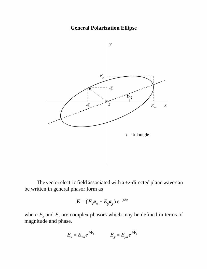
General Polarization Ellipse

The vector electric field associated with a +z-directed plane wave canbe written in general phasor form as

where Ex and Ey are complex phasors which may be defined in terms ofmagnitude and phase.

x (z, t)

x (z, t)

y (z, t)

y (z, t)

The instantaneous components of the electric field are found bymultiplying the phasor components by e j t and taking the real part.

The relative positions of the instantaneous electric field components on thegeneral polarization ellipse defines the polarization of the plane wave.

Linear Polarization

If we define the phase shift between the two electric fieldcomponents as

we find that a phase shift of

defines a linearly polarized wave.

Examples of linear polarization:

If Eyo = 0 Linear polarization in the x-direction ( = 0)If Exo = 0 Linear polarization in the y-direction ( = 90o)If Exo = Eyo and n is even Linear polarization ( = 45o)If Exo = Eyo and n is odd Linear polarization ( = 135o)

x (z, t)

x (z, t)

y (z, t)

y (z, t)

Circular Polarization

If Exo = Eyo and

then

This is left-hand circular polarization.

If Exo = Eyo and

then

This is right-hand circular polarization.

Elliptical Polarization

Elliptical polarization follows definitions as circular polarizationexcept that Exo Eyo.

Exo Eyo, = (2n+½) left-hand elliptical polarization Exo Eyo, = (2n+½) right-hand elliptical polarization

Antenna Equivalent Areas

Antenna Effective Aperture (Area)

Given a receiving antenna oriented for maximum response,polarization matched to the incident wave, and impedance matched to itsload, the resulting power delivered to the receiver (Prec) may be defined interms of the antenna effective aperture (Ae) as

where S is the power density of the incident wave (magnitude of thePoynting vector) defined by

According to the equivalent circuit under matched conditions,

We may solve for the antenna effective aperture which gives

Antenna Scattering Area

The total power scattered by the receiving antenna is defined as theproduct of the incident power density and the antenna scattering area (As).

From the equivalent circuit, the total scattered power is

which gives

Antenna Loss Area

The total power dissipated as heat by the receiving antenna is definedas the product of the incident power density and the antenna loss area(AL).

From the equivalent circuit, the total dissipated power is

which gives

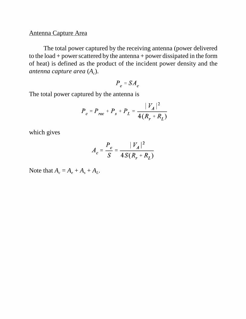
Antenna Capture Area

The total power captured by the receiving antenna (power deliveredto the load + power scattered by the antenna + power dissipated in the formof heat) is defined as the product of the incident power density and theantenna capture area (Ac).

The total power captured by the antenna is

which gives

Note that Ac = Ae + As + AL.

Maximum Directivity and Effective Aperture

Assume the transmitting and receiving antennas are lossless andoriented for maximum response.

Aet, Dot - transmit antenna effective aperture and maximum directivityAer, Dor - receive antenna effective aperture and maximum directivity

If we assume that the total power transmitted by the transmit antenna is Pt,the power density at the receive antenna (Wr) is

The total power received by the receive antenna (Pr) is

which gives

If we interchange the transmit and receive antennas, the previousequation still holds true by interchanging the respective transmit andreceive quantities (assuming a linear, isotropic medium), which gives

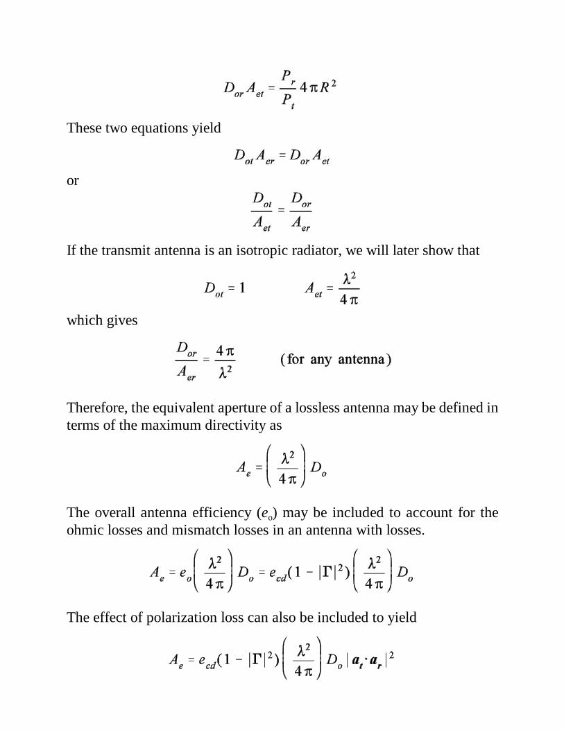
These two equations yield

or

If the transmit antenna is an isotropic radiator, we will later show that

which gives

Therefore, the equivalent aperture of a lossless antenna may be defined interms of the maximum directivity as

The overall antenna efficiency (eo) may be included to account for theohmic losses and mismatch losses in an antenna with losses.

The effect of polarization loss can also be included to yield

Effective Area and Gain___________________________________________________________________________________Hon Tat Hui

1

Proof of ( ) ( ) ( )φθπλ

=φθπλ

=φθ ,g4

,D4

,A22

e

Extracted from the book: Kai Fong Lee, Principles of Antenna Theory, John Wiley & Sons, 1984, pp. 74-76.

Effective Area and Gain___________________________________________________________________________________Hon Tat Hui

2

Friis Transmission Equation

The Friis transmission equation defines the relationship betweentransmitted power and received power in an arbitrary transmit/receiveantenna system. Given arbitrarily oriented transmitting and receivingantennas, the power density at the receiving antenna (Wr) is

where Pt is the input power at the terminals of the transmit antenna andwhere the transmit antenna gain and directivity for the system performanceare related by the overall efficiency

where ecdt is the radiation efficiency of the transmit antenna and t is thereflection coefficient at the transmit antenna terminals. Notice that thisdefinition of the transmit antenna gain includes the mismatch losses for thetransmit system in addition to the conduction and dielectric losses. Amanufacturer’s specification for the antenna gain will not include themismatch losses.

The total received power delivered to the terminals of the receivingantenna (Pr) is

where the effective aperture of the receiving antenna (Aer) must take into

account the orientation of the antenna. We may extend our previousdefinition of the antenna effective aperture (obtained using the maximumdirectivity) to a general effective aperture for any antenna orientation.

The total received power is then

such that the ratio of received power to transmitted power is

Including the polarization losses yields

For antennas aligned for maximum response, reflection-matched andpolarization matched, the Friis transmission equation reduces to

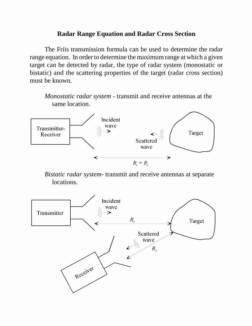
Radar Range Equation and Radar Cross Section

The Friis transmission formula can be used to determine the radarrange equation. In order to determine the maximum range at which a giventarget can be detected by radar, the type of radar system (monostatic orbistatic) and the scattering properties of the target (radar cross section)must be known.

Monostatic radar system - transmit and receive antennas at thesame location.

Bistatic radar system- transmit and receive antennas at separatelocations.

Radar cross section (RCS) - a measure of the ability of a target to reflect(scatter) electromagnetic energy (units = m2). The area which interceptsthat amount of total power which, when scattered isotropically,produces the same power density at the receiver as the actual target.

If we define = radar cross section (m2)Wi = incident power density at the target (W/m2)Pc = equivalent power captured by the target (W)Ws = scattered power density at the receiver (W/m2)

According to the definition of the target RCS, the relationship between theincident power density at the target and the scattered power density at thereceive antenna is

The limit is usually included since we must be in the far-field of the targetfor the radar cross section to yield an accurate result.

The radar cross section may be written as

where (Ei, Hi) are the incident electric and magnetic fields at the target and(Es, Hs) are the scattered electric and magnetic fields at the receiver. Theincident power density at the target generated by the transmitting antenna(Pt, Gt, Dt, eot, t, at) is given by

The total power captured by the target (Pc) is

The power captured by the target is scattered isotropically so that thescattered power density at the receiver is

The power delivered to the receiving antenna load is

Showing the conduction losses, mismatch losses and polarization lossesexplicitly, the ratio of the received power to transmitted power becomes

where

aw - polarization unit vector for the scattered wavesar - polarization unit vector for the receive antenna

Given matched antennas aligned for maximum response and polarizationmatched, the general radar range equation reduces to

Example

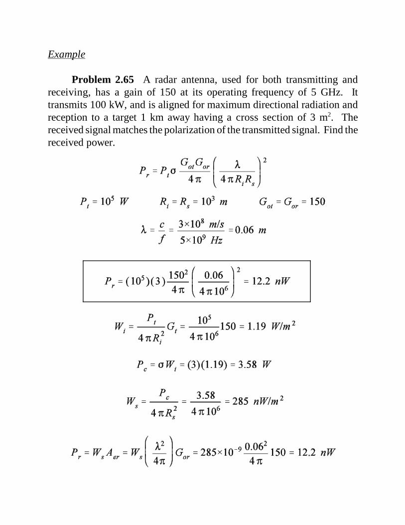
Problem 2.65 A radar antenna, used for both transmitting andreceiving, has a gain of 150 at its operating frequency of 5 GHz. Ittransmits 100 kW, and is aligned for maximum directional radiation andreception to a target 1 km away having a cross section of 3 m2. Thereceived signal matches the polarization of the transmitted signal. Find thereceived power.

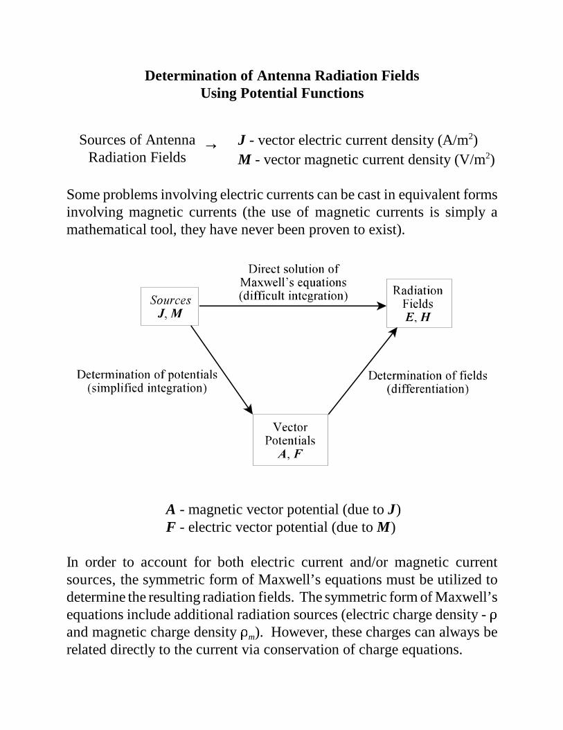
Determination of Antenna Radiation FieldsUsing Potential Functions

J - vector electric current density (A/m2)M - vector magnetic current density (V/m2)

Some problems involving electric currents can be cast in equivalent formsinvolving magnetic currents (the use of magnetic currents is simply amathematical tool, they have never been proven to exist).

A - magnetic vector potential (due to J)F - electric vector potential (due to M)

In order to account for both electric current and/or magnetic currentsources, the symmetric form of Maxwell’s equations must be utilized todetermine the resulting radiation fields. The symmetric form of Maxwell’sequations include additional radiation sources (electric charge density - and magnetic charge density m). However, these charges can always berelated directly to the current via conservation of charge equations.

Sources of AntennaRadiation Fields

Maxwell’s equations (symmetric, time-harmonic form)

The use of potentials in the solution of radiation fields employs the conceptof superposition of fields.

Electric current

Magnetic vector

Radiation fields source (J, ) potential (A) (EA, HA)

Magnetic current

Electric vector

Radiation fields source (M, m) potential (F) (EF, HF)

The total radiation fields (E, H) are the sum of the fields due to electriccurrents (EA, HA) and the fields due to the magnetic currents (EF, HF).

Maxwell’s Equations (electric sources only F = 0)

Maxwell’s Equations (magnetic sources only A = 0)

Based on the vector identity,

any vector with zero divergence (rotational or solenoidal field) can beexpressed as the curl of some other vector. From Maxwell’s equations withelectric or magnetic sources only [Equations (1d) and (2c)], we find

so that we may define these vectors as

where A and F are the magnetic and electric vector potentials, respectively.The flux density definitions in Equations (3a) and (3b) lead to thefollowing field definitions:

Inserting (3a) into (1a) and (3b) into (2b) yields

Equations (5a) and (5b) can be rewritten as

Based on the vector identity

the bracketed terms in (6a) and (6b) represent non-solenoidal (lamellar orirrotational fields) and may each be written as the gradient of some scalar

where e is the electric scalar potential and m is the magnetic scalarpotential. Solving equations (7a) and (7b) for the electric and magneticfields yields

Equations (4a) and (8a) give the fields (EA, HA) due to electric sourceswhile Equations (4b) and (8b) give the fields (EF, HF) due to magneticsources. Note that these radiated fields are obtained by differentiating therespective vector and scalar potentials.

The integrals which define the vector and scalar potential can befound by first taking the curl of both sides of Equations (4a) and (4b):

According to the vector identity

and Equations (1b) and (2a), we find

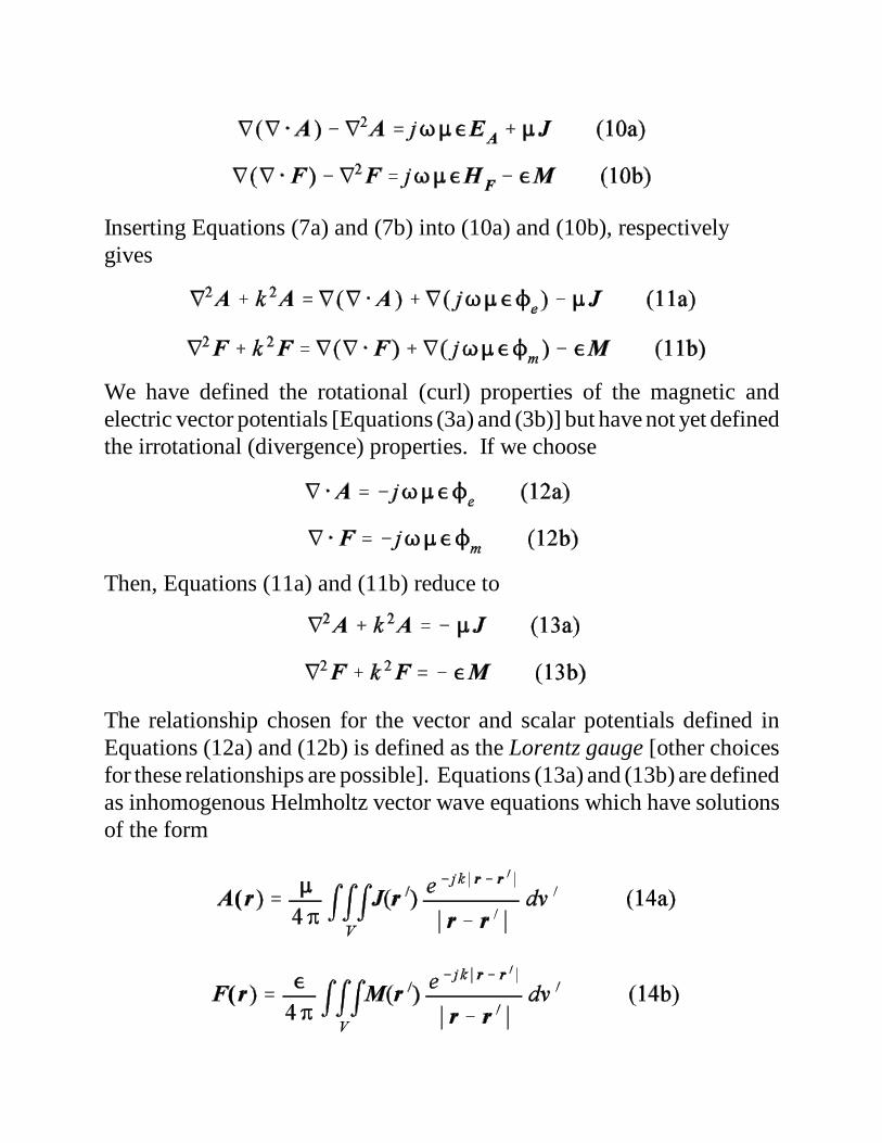
Inserting Equations (7a) and (7b) into (10a) and (10b), respectivelygives

We have defined the rotational (curl) properties of the magnetic andelectric vector potentials [Equations (3a) and (3b)] but have not yet definedthe irrotational (divergence) properties. If we choose

Then, Equations (11a) and (11b) reduce to

The relationship chosen for the vector and scalar potentials defined inEquations (12a) and (12b) is defined as the Lorentz gauge [other choicesfor these relationships are possible]. Equations (13a) and (13b) are definedas inhomogenous Helmholtz vector wave equations which have solutionsof the form

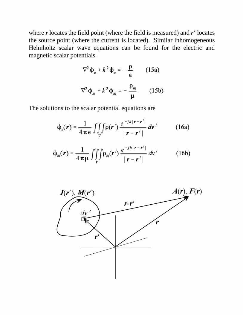
where r locates the field point (where the field is measured) and r locatesthe source point (where the current is located). Similar inhomogeneousHelmholtz scalar wave equations can be found for the electric andmagnetic scalar potentials.

The solutions to the scalar potential equations are

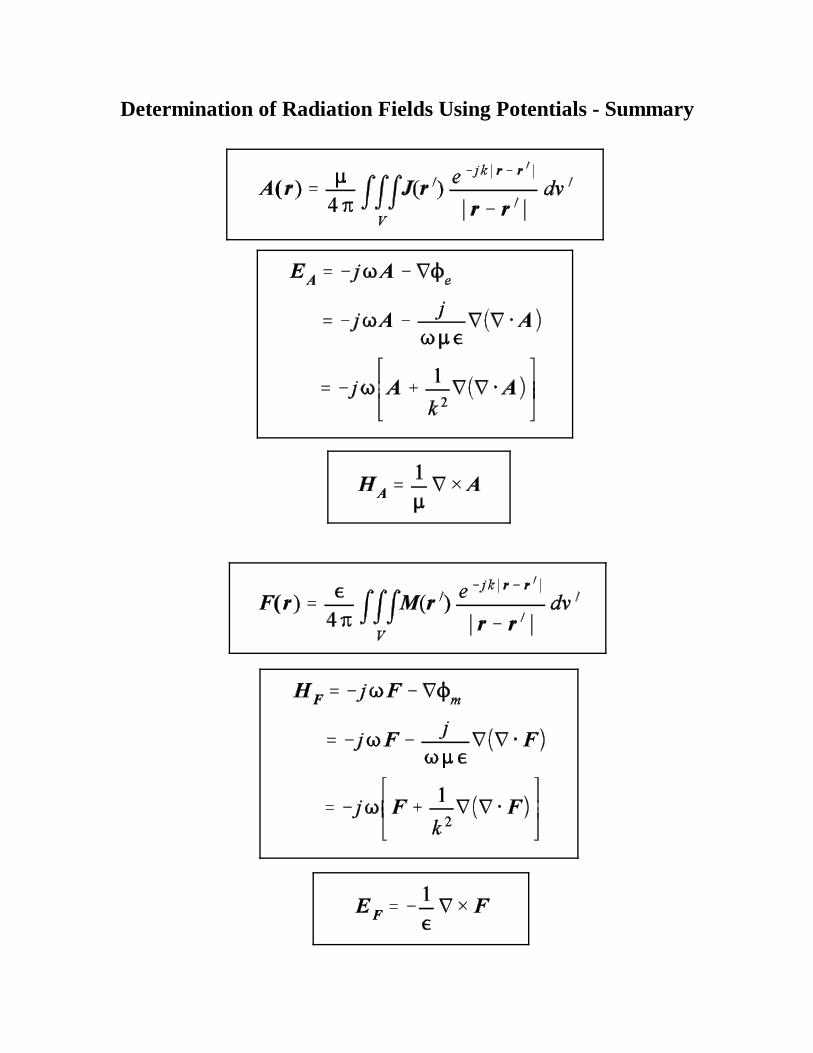
Determination of Radiation Fields Using Potentials - Summary

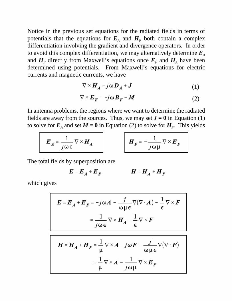
Notice in the previous set equations for the radiated fields in terms ofpotentials that the equations for EA and HF both contain a complexdifferentiation involving the gradient and divergence operators. In orderto avoid this complex differentiation, we may alternatively determine EA

and HF directly from Maxwell’s equations once EF and HA have beendetermined using potentials. From Maxwell’s equations for electriccurrents and magnetic currents, we have

In antenna problems, the regions where we want to determine the radiatedfields are away from the sources. Thus, we may set J = 0 in Equation (1)to solve for EA and set M = 0 in Equation (2) to solve for HF. This yields

The total fields by superposition are

which gives

(1)

(2)

(1)

Antenna Far Fields in Terms of Potentials

As shown previously, the magnetic vector potential and electricvector potentials are defined as integrals of the (antenna) electric ormagnetic current density.

If we are interested in determining the antenna far fields, then we mustdetermine the potentials in the far field. We will find that the integralsdefining the potentials simplify in the far field. In the far field, the vectorsr and r r becomes nearly parallel.

(2)

(3)

(4)

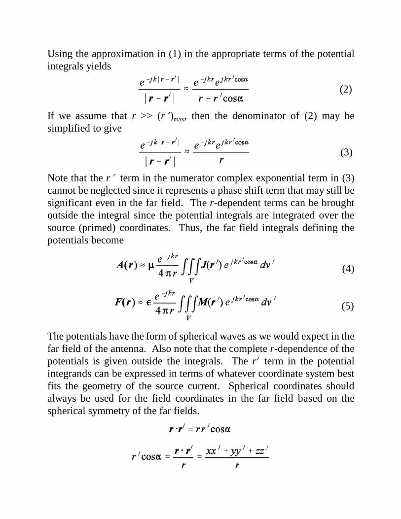
Using the approximation in (1) in the appropriate terms of the potentialintegrals yields

If we assume that r >> (r )max, then the denominator of (2) may besimplified to give

Note that the r term in the numerator complex exponential term in (3)cannot be neglected since it represents a phase shift term that may still besignificant even in the far field. The r-dependent terms can be broughtoutside the integral since the potential integrals are integrated over thesource (primed) coordinates. Thus, the far field integrals defining thepotentials become

The potentials have the form of spherical waves as we would expect in thefar field of the antenna. Also note that the complete r-dependence of thepotentials is given outside the integrals. The r term in the potentialintegrands can be expressed in terms of whatever coordinate system bestfits the geometry of the source current. Spherical coordinates shouldalways be used for the field coordinates in the far field based on thespherical symmetry of the far fields.

(5)

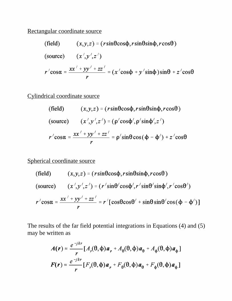
Rectangular coordinate source

Cylindrical coordinate source

Spherical coordinate source

The results of the far field potential integrations in Equations (4) and (5)may be written as

(6)

(7)

(8)

(9)

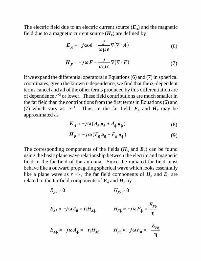
The electric field due to an electric current source (EA) and the magneticfield due to a magnetic current source (HF) are defined by

If we expand the differential operators in Equations (6) and (7) in sphericalcoordinates, given the known r-dependence, we find that the ar-dependentterms cancel and all of the other terms produced by this differentiation areof dependence r2 or lower. These field contributions are much smaller inthe far field than the contributions from the first terms in Equations (6) and(7) which vary as r1. Thus, in the far field, EA and HF may beapproximated as

The corresponding components of the fields (HA and EF) can be foundusing the basic plane wave relationship between the electric and magneticfield in the far field of the antenna. Since the radiated far field mustbehave like a outward propagating spherical wave which looks essentiallylike a plane wave as r , the far field components of HA and EF arerelated to the far field components of EA and HF by

Solving the previous equations for the individual components of HA andEF yields

Thus, once the far field potential integral is evaluated, the correspondingfar field can be found using the simple algebraic formulas above (thedifferentiation has already been performed).

Duality

Duality - If the equations governing two different phenomena areidentical in mathematical form, then the solutions also take on the samemathematical form (dual quantities).

Dual Equations

Electric Sources Magnetic Sources

Dual Quantities

Electric Sources Magnetic Sources

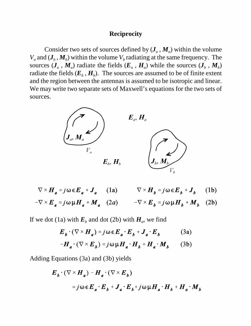
Reciprocity

Consider two sets of sources defined by (Ja , Ma) within the volumeVa and (Jb , Mb) within the volume Vb radiating at the same frequency. Thesources (Ja , Ma) radiate the fields (Ea , Ha) while the sources (Jb , Mb)radiate the fields (Eb , Hb). The sources are assumed to be of finite extentand the region between the antennas is assumed to be isotropic and linear.We may write two separate sets of Maxwell’s equations for the two sets ofsources.

If we dot (1a) with Eb and dot (2b) with Ha, we find

Adding Equations (3a) and (3b) yields

The previous equation may be rewritten using the following vector identity.

which gives

If we dot (1b) with Ea and dot (2a) with Hb, and perform the sameoperations, then we find

Subtracting (4a) from (4b) gives

If we integrate both sides of Equation (5) throughout all space and applythe divergence theorem to the left hand side, then

The surface on the left hand side of Equation (6) is a sphere of infiniteradius on which the radiated fields approach zero. The volume V includesall space. Therefore, we may write

Note that the left hand side of the previous integral depends on the “b” setof sources while the right hand side depends on the “a” set of sources.Since we have limited the sources to the volumes Va and Vb, we may limitthe volume integrals in (7) to the respective source volumes so that

Equation (8) represents the general form of the reciprocity theorem. We may use the reciprocity theorem to analyze a transmitting-

receiving antenna system. Consider the antenna system shown below. Formathematical simplicity, let’s assume that the antennas are perfectly-conducting, electrically short dipole antennas.

The source integrals in the general 3-D reciprocity theorem of Equation (8)simplify to line integrals for the case of wire antennas.

Furthermore, the electric field along the perfectly conducting wire is zeroso that the integration can be reduced to the antenna terminals (gaps).

If we further assume that the antenna current is uniform over theelectrically short dipole antennas, then

The line integral of the electric field transmitted by the opposite antennaover the antenna terminal gives the resulting induced open circuit voltage.

If we write the two port equations for the antenna system, we find

Note that the impedances Zab and Zba have been shown to be equal from thereciprocity theorem.

Therefore, if we place a current source on antenna a and measure theresponse at antenna b, then switch the current source to antenna b andmeasure the response at antenna a, we find the same response (magnitudeand phase). Also, since the transfer impedances (Zab and Zba) are identical,the transmit and receive patterns of a given antenna are identical. Thus, wemay measure the pattern of a given antenna in either the transmitting modeor receiving mode, whichever is more convenient.

Wire Antennas

Electrical Size of an Antenna - the physical dimensions of the antennadefined relative to wavelength.

Electrically small antenna - the dimensions of the antenna are smallrelative to wavelength.

Electrically large antenna - the dimensions of the antenna are largerelative to wavelength.

Example Consider a dipole antenna of length L = 1m. Determine theelectrical length of the dipole at f = 3 MHz and f = 30 GHz.

f = 3 MHz f = 30 GHz ( = 100m) ( = 0.01m) Electrically small Electrically large

Infinitesimal Dipole(l /50, a << )

We assume that the axial current along the infinitesimal dipole isuniform. With a << , we may assume that any circumferential currentsare negligible and treat the dipole as a current filament.

The infinitesimal dipole with a constant current along its length is a non-physical antenna. However, the infinitesimal dipole approximates severalphysically realizable antennas.

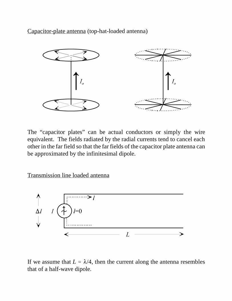
Capacitor-plate antenna (top-hat-loaded antenna)

The “capacitor plates” can be actual conductors or simply the wireequivalent. The fields radiated by the radial currents tend to cancel eachother in the far field so that the far fields of the capacitor plate antenna canbe approximated by the infinitesimal dipole.

Transmission line loaded antenna

If we assume that L /4, then the current along the antenna resemblesthat of a half-wave dipole.

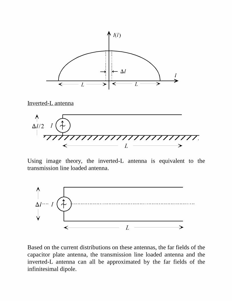
Inverted-L antenna

Using image theory, the inverted-L antenna is equivalent to thetransmission line loaded antenna.

Based on the current distributions on these antennas, the far fields of thecapacitor plate antenna, the transmission line loaded antenna and theinverted-L antenna can all be approximated by the far fields of theinfinitesimal dipole.

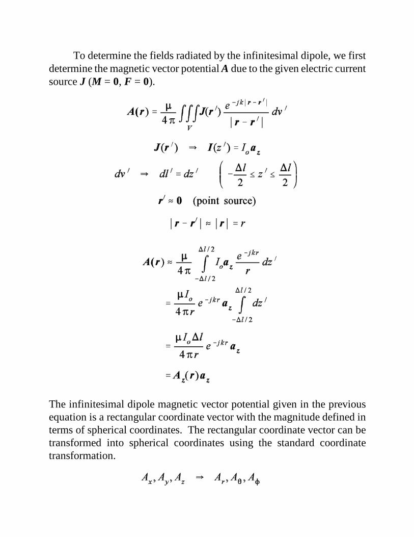
To determine the fields radiated by the infinitesimal dipole, we firstdetermine the magnetic vector potential A due to the given electric currentsource J (M = 0, F = 0).

The infinitesimal dipole magnetic vector potential given in the previousequation is a rectangular coordinate vector with the magnitude defined interms of spherical coordinates. The rectangular coordinate vector can betransformed into spherical coordinates using the standard coordinatetransformation.

The total magnetic vector potential may then be written in vector form as

Because of the true point source nature of the infinitesimal dipole (l /50), the equation above for the magnetic vector potential of theinfinitesimal dipole is valid everywhere. We may use this expression forA to determine both near fields and far fields.

The radiated fields of the infinitesimal dipole are found bydifferentiating the magnetic vector potential.

The electric field is found using either potential theory or Maxwell’sequations.

Potential Theory

Maxwell’s Equations (J = 0 away from the source)

Note that electric field expression in terms of potentials requires two levelsof differentiation while the Maxwell’s equations equation requires only onelevel of differentiation. Thus, using Maxwell’s equations, we find

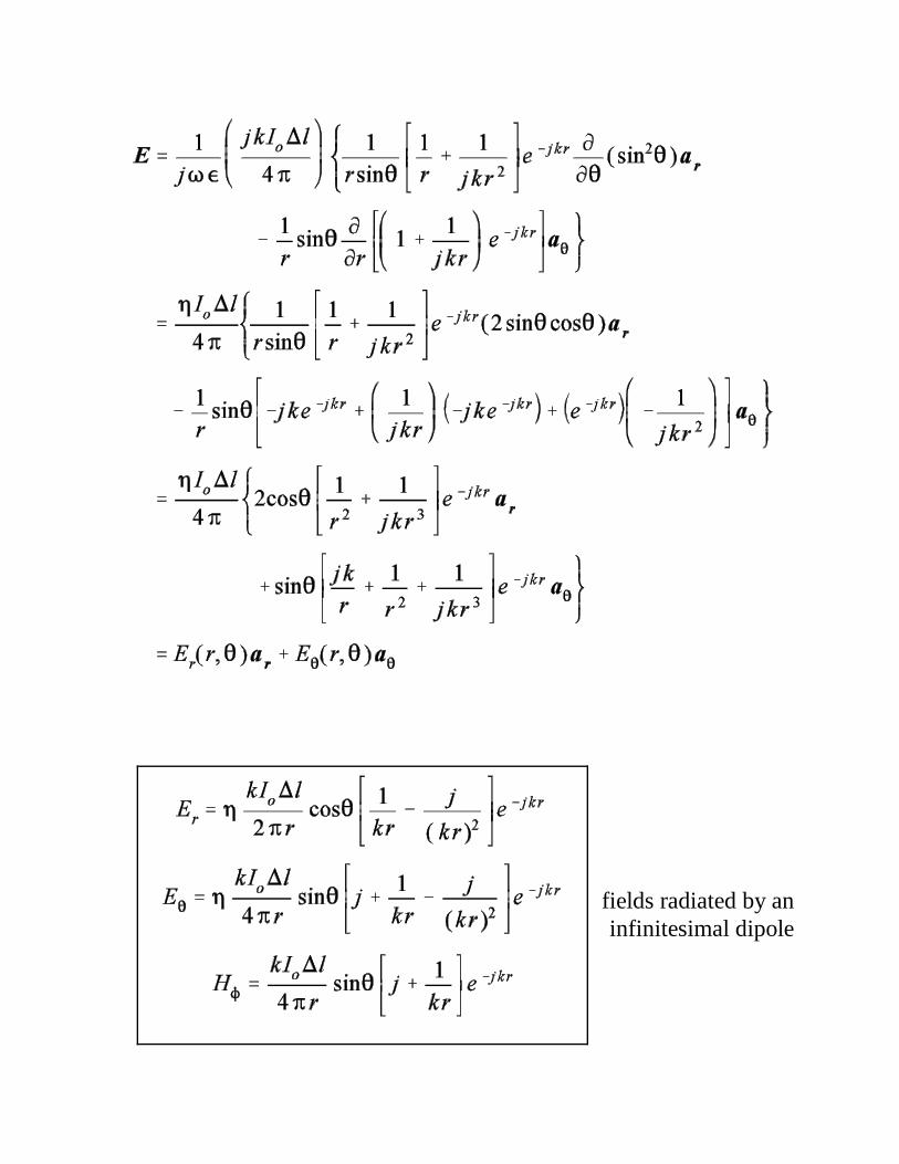
fields radiated by an infinitesimal dipole

Field Regions of the Infinitesimal Dipole

We may separate the fields of the infinitesimal dipole into the threestandard regions:

Reactive near field kr << 1 Radiating near field kr > 1 Far field kr >> 1

Considering the bracketed terms [ ] in the radiated field expressions for theinfinitesimal dipole ...

Reactive near field (kr << 1) (kr)-2 terms dominate Radiating near field (kr > 1) constant terms dominate if present

otherwise, (kr)-1 terms dominate Far field (kr >> 1) constant terms dominate

0 2 4 6 8 10 120

0.5

1

1.5

2

2.5

3

3.5

4

4.5

5

Reactive near field [ kr << 1 or r << /2 ]

When kr << 1, the terms which vary inversely with the highest powerof kr are dominant. Thus, the near field of the infinitesimal dipole is givenby

Infinitesimal dipole near fields

Note the 90o phase difference between the electric field components andthe magnetic field component (these components are in phase quadrature)which indicates reactive power (stored energy, not radiation). If weinvestigate the Poynting vector of the dominant near field terms, we find

The Poynting vector (complex vector power density) for the infinitesimaldipole near field is purely imaginary. An imaginary Poynting vectorcorresponds to standing waves or stored energy (reactive power).

The vector form of the near electric field is the same as that for anelectrostatic dipole (charges +q and q separated by a distance l).

If we replace the term (Io/k) by in the near electric field terms by itscharge equivalent expression, we find

The electric field expression above is identical to that of the electrostaticdipole except for the complex exponential term (the infinitesimal dipoleelectric field oscillates). This result is related to the assumption of auniform current over the length of the infinitesimal dipole. The only wayfor the current to be uniform, even at the ends of the wire, is for charge tobuild up and decay at the ends of the dipole as the current oscillates.

The near magnetic field of the infinitesimal dipole can be shown tobe mathematically equivalent to that of a short DC current segmentmultiplied by the same complex exponential term.

Radiating near field [ kr 1 or r /2 ]

The dominant terms for the radiating near field of the infinitesimaldipole are the terms which are constant with respect to kr for E and H

and the term proportional to (kr)-1 for Er.

Infinitesimal dipole radiating near field

Note that E and H are now in phase which yields a Poynting vector forthese two components which is purely real (radiation). The direction ofthis component of the Poynting vector is outward radially denoting theoutward radiating real power.

Far field [ kr >> 1 or r >> /2 ]

The dominant terms for the far field of the infinitesimal dipole are theterms which are constant with respect to kr.

Infinitesimal dipole far field

Note that the far field components of E and H are the same twocomponents which produced the radially-directed real-valued Poyntingvector (radiated power) for the radiating near field. Also note that there isno radial component of E or H so that the propagating wave is a transverseelectromagnetic (TEM) wave. For very large values of r, this TEM waveapproaches a plane wave. The ratio of the far electric field to the farmagnetic field for the infinitesimal dipole yields the intrinsic impedanceof the medium.

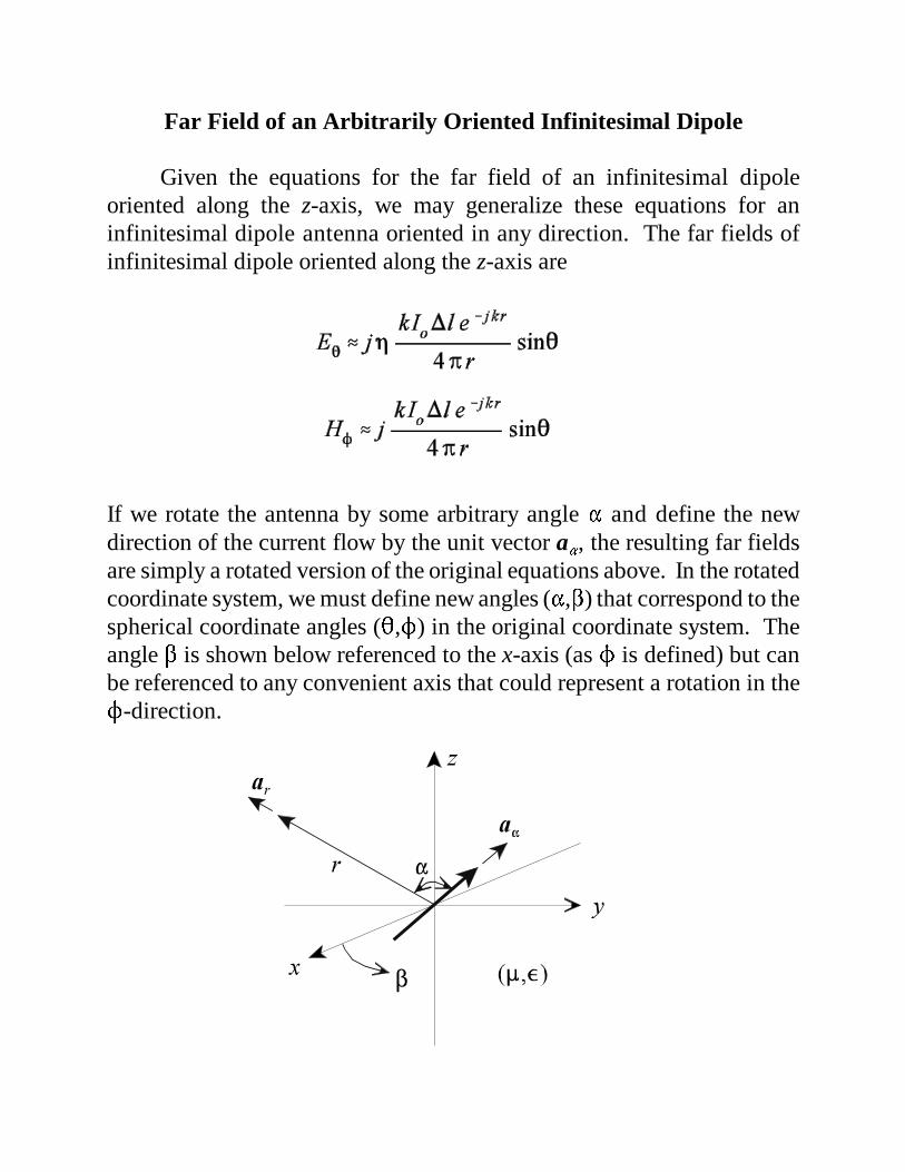
Far Field of an Arbitrarily Oriented Infinitesimal Dipole

Given the equations for the far field of an infinitesimal dipoleoriented along the z-axis, we may generalize these equations for aninfinitesimal dipole antenna oriented in any direction. The far fields ofinfinitesimal dipole oriented along the z-axis are

If we rotate the antenna by some arbitrary angle and define the newdirection of the current flow by the unit vector a, the resulting far fieldsare simply a rotated version of the original equations above. In the rotatedcoordinate system, we must define new angles (,) that correspond to thespherical coordinate angles (,) in the original coordinate system. Theangle is shown below referenced to the x-axis (as is defined) but canbe referenced to any convenient axis that could represent a rotation in the-direction.

Note that the infinitesimal far fields in the original coordinate systemdepend on the spherical coordinates r and . The value of r is identical inthe two coordinates systems since it represents the distance from thecoordinate origin. However, we must determine the transformation from to . The transformations of the far fields in the original coordinatesystem to those in the rotated coordinate system can be written as

Specifically, we need the definition of sin. According to thetrigonometric identity

we may write

Based on the definition of the dot product, the cos term may be writtenas

so that

Inserting our result for the sin term yields

Example

Determine the far fields of an infinitesimal dipole oriented along they-axis.

Poynting’s Theorem (Conservation of Power)

Poynting’s theorem defines the basic principle of conservation ofpower which may be applied to radiating antennas. The derivation of thetime-harmonic form of Poynting’s vector begins with the following vectoridentity

If we insert the Poynting vector (S = E × H*) in the left hand side of theabove identity, we find

From Maxwell’s equations, the curl of E and H are

such that

Integrating both sides of this equation over any volume V and applying thedivergence theorem to the left hand side gives

The current density in the equation above consists of two components: theimpressed (source) current (Ji) and the conduction current (Jc).

Inserting the current expression and dividing both sides of the equation by2 yields Poynting’s theorem.

The individual terms in the above equation may be identified as

Poynting’s theorem may then be written as

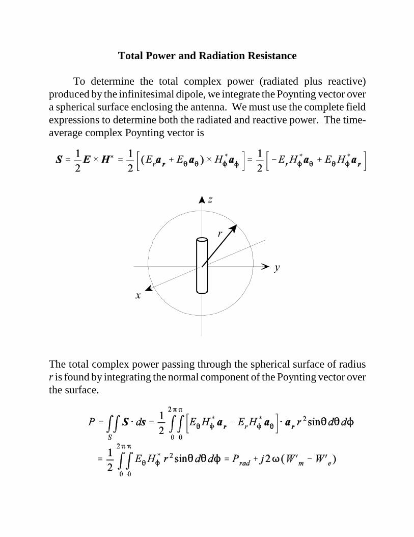
Total Power and Radiation Resistance

To determine the total complex power (radiated plus reactive)produced by the infinitesimal dipole, we integrate the Poynting vector overa spherical surface enclosing the antenna. We must use the complete fieldexpressions to determine both the radiated and reactive power. The time-average complex Poynting vector is

The total complex power passing through the spherical surface of radiusr is found by integrating the normal component of the Poynting vector overthe surface.

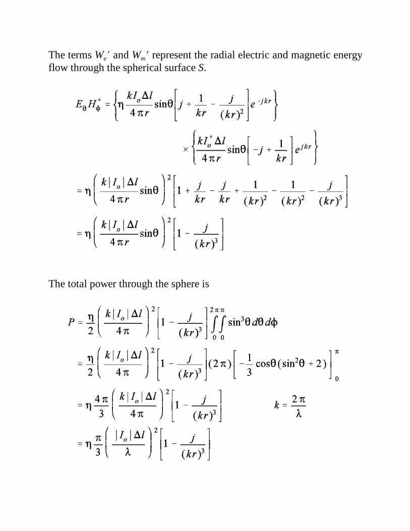
The terms We and Wm represent the radial electric and magnetic energyflow through the spherical surface S.

The total power through the sphere is

The real and imaginary parts of the complex power are

The radiation resistance for the infinitesimal dipole is found according to

Infinitesimal dipole radiation resistance

Infinitesimal Dipole Radiation Intensity and Directivity

The radiation intensity of the infinitesimal dipole may be found byusing the previously determined total fields.

Infinitesimal dipole directivity function Infinitesimal dipole Maximum directivity

Infinitesimal Dipole Effective Aperture and Solid Beam Angle

The effective aperture of the infinitesimal dipole is found from themaximum directivity:

Infinitesimal dipole effective aperture

The beam solid angle for the infinitesimal dipole can be found from themaximum directivity,

or can be determined directly from the radiation intensity function.

Infinitesimal dipole beam solid angle

Short Dipole(/50 l /10, a <<)

Note that the magnetic vector potential of the short dipole (length = l, peakcurrent = Io) is one half that of the equivalent infinitesimal dipole (lengthl = l, current = Io).

The average current on the short dipole is one half that of the equivalentinfinitesimal dipole. Therefore, the fields produced by the short dipole areexactly one half those produced by the equivalent infinitesimal dipole.

Short dipole radiated fields

Short dipole near fields

Short dipole radiating near field

Short dipole far field

Since the fields produced by the short dipole are one half those of theequivalent infinitesimal dipole, the real power radiated by the short dipoleis one fourth that of the infinitesimal dipole. Thus, Prad for the short dipoleis

and the associated radiation resistance is

Short dipole radiation resistance

The directivity function, the maximum directivity, effective area and beamsolid angle of the short dipole are all identical to the corresponding valuefor the infinitesimal dipole.

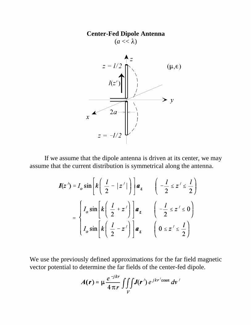
Center-Fed Dipole Antenna(a << )

If we assume that the dipole antenna is driven at its center, we mayassume that the current distribution is symmetrical along the antenna.

We use the previously defined approximations for the far field magneticvector potential to determine the far fields of the center-fed dipole.

field coordinates (spherical)

Source coordinates (rectangular)

For the center-fed dipole lying along the z-axis, x = y = 0, so that

Transforming the z-directed vector potential to spherical coordinates gives

(Center-fed dipole far field magnetic vector potential )

The far fields of the center-fed dipole in terms of the magnetic vectorpotential are

(Center-fed dipole far field electric field)

(Center-fed dipole far field magnetic field)

The time-average complex Poynting vector in the far field of the center-feddipole is

The radiation intensity function for the center-fed dipole is given by

(Center-fed dipole radiation intensity function)

We may plot the normalized radiation intensity function [U() = BoF()]to determine the effect of the antenna length on its radiation pattern.

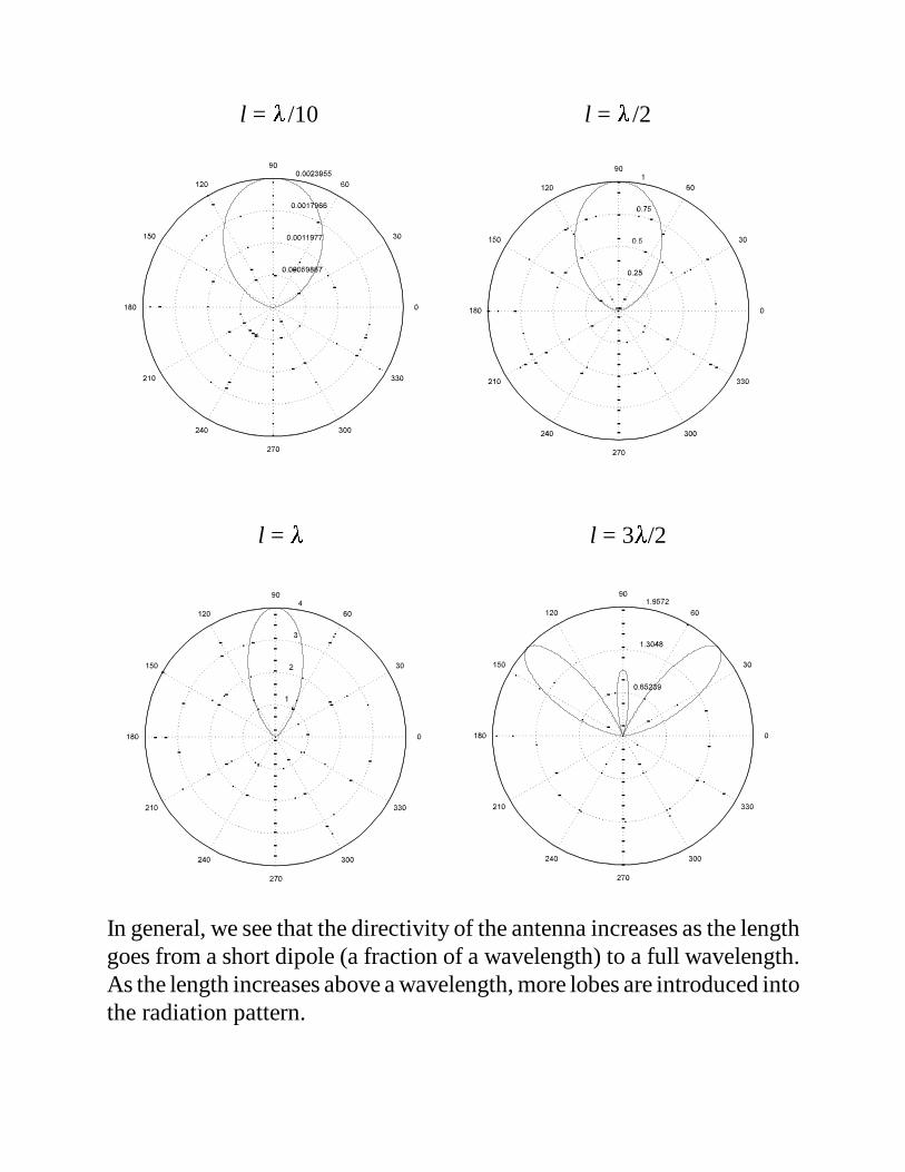
l = /10 l = /2

l = l = 3/2

In general, we see that the directivity of the antenna increases as the lengthgoes from a short dipole (a fraction of a wavelength) to a full wavelength.As the length increases above a wavelength, more lobes are introduced intothe radiation pattern.

-0.05 -0.04 -0.03 -0.02 -0.01 0 0.01 0.02 0.03 0.04 0.050

0.1

0.2

0.3

0.4

0.5

0.6

0.7

0.8

0.9

1

z/λ

I(z)

/ I o

-0.25 -0.2 -0.15 -0.1 -0.05 0 0.05 0.1 0.15 0.2 0.250

0.1

0.2

0.3

0.4

0.5

0.6

0.7

0.8

0.9

1

z/λ

I(z)

/ I o

-0.5 -0.4 -0.3 -0.2 -0.1 0 0.1 0.2 0.3 0.4 0.50

0.1

0.2

0.3

0.4

0.5

0.6

0.7

0.8

0.9

1

z/λ

I(z)

/ I o

-0.6 -0.4 -0.2 0 0.2 0.4 0.6-1

-0.8

-0.6

-0.4

-0.2

0

0.2

0.4

0.6

0.8

1

z/λ

I(z)

/ I o

l = /10 l = /2

l = l = 3/2

The total real power radiated by the center-fed dipole is

The -dependent integral in the radiated power expression cannot beintegrated analytically. However, the integral may be manipulated, usingseveral transformations of variables, into a form containing somecommonly encountered special functions (integrals) known as the sineintegral and cosine integral.

The radiated power of the center-fed dipole becomes

The radiated power is related to the radiation resistance of the antenna by

which gives

(Center-fed dipole radiation resistance)

The directivity function of the center-fed dipole is given by

Center-fed dipole directivity function

The maximum directivity is

Center-fed dipole maximum directivity

The effective aperture is

Center-fed dipole effective aperture

Center-fed dipole Solid beam angle

Half-Wave Dipole

Center-fedhalf-wave dipole far fields

Center-fed half-wave dipole radiation intensity function

Center-fed half-wave dipole radiation resistance (in air)

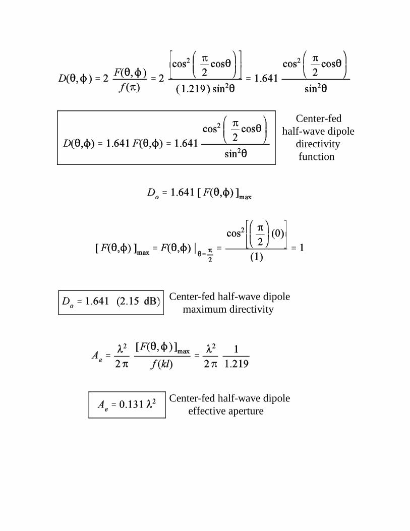
Center-fed half-wave dipole directivity function

Center-fed half-wave dipole maximum directivity

Center-fed half-wave dipole effective aperture

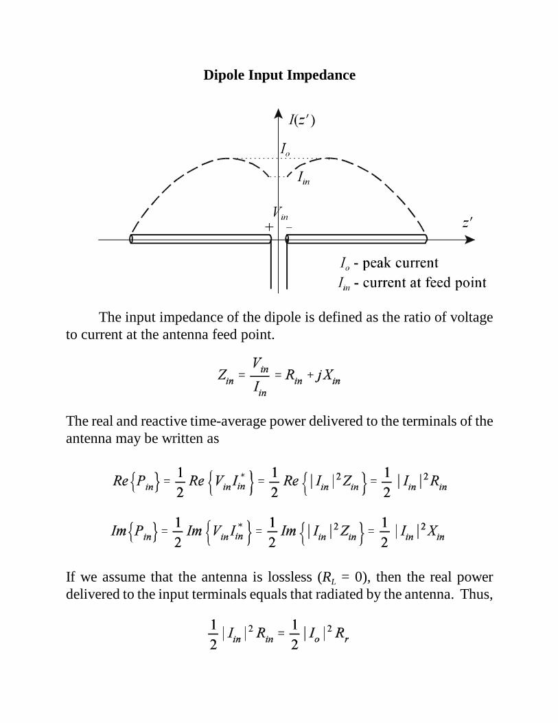
Dipole Input Impedance

The input impedance of the dipole is defined as the ratio of voltageto current at the antenna feed point.

The real and reactive time-average power delivered to the terminals of theantenna may be written as

If we assume that the antenna is lossless (RL = 0), then the real powerdelivered to the input terminals equals that radiated by the antenna. Thus,

and the antenna input resistance is related to the antenna radiationresistance by

In a similar fashion, we may equate the reactive power delivered to theantenna input terminals to that stored in the near field of the antenna.

or

The general dipole current is defined by

The current Iin is the current at the feed point of the dipole (z = 0) so that

The input resistance and reactance of the antenna are then related to theequivalent circuit values of radiation resistance and the antenna reactanceby

The dipole reactance may be determined in closed form using a techniqueknown as the induced EMF method (Chapter 8) but requires that the radiusof the wire (a) be included. The resulting dipole reactance is

(Center-fed dipole reactance)

The input resistance and reactance are plotted in Figure 8.16 (p.411) for adipole of radius a = 10-5

. If the dipole is 0.5 in length, the inputimpedance is found to be approximately (73 + j42.5) . The first dipoleresonance (Xin = 0) occurs when the dipole length is slightly less than one-half wavelength. The exact resonant length depends on the wire radius, butfor wires that are electrically very thin, the resonant length of the dipole isapproximately 0.48. As the wire radius increases, the resonant lengthdecreases slightly [see Figure 8.17 (p.412)].

Antenna and Scatterers

All of the antennas considered thus far have been assumed to beradiating in a homogeneous medium of infinite extent. When an antennaradiates in the presence of a conductor(inhomogeneous medium), currentsare induced on the conductor which re-radiate (scatter) additional fields.The total fields produced by an antenna in the presence of a scatterer arethe superposition of the original radiated fields (incident fields, [E inc,H inc]those produced by the antenna in the absence of the scatterer) plus thefields produced by the currents induced on the scatterer (scattered fields,[E scat,H scat]).

To evaluate the total fields, we must first determine the scatteredfields which depend on the currents flowing on the scatterer. Thedetermination of the scatterer currents typically requires a numericalscheme (integral equation in terms of the scatterer currents or a differentialequation in the form of a boundary value problem). However, for simplescatterer shapes, we may use image theory to simplify the problem.

Image Theory

Given an antenna radiating over a perfect conducting ground plane,[perfect electric conductor (PEC), perfect magnetic conductor (PMC)] wemay use image theory to formulate the total fields without ever having todetermine the surface currents induced on the ground plane. Image theoryis based on the electric or magnetic field boundary condition on the surfaceof the perfect conductor (the tangential electric field is zero on the surfaceof a PEC, the tangential magnetic field is zero on the surface of a PMC).Using image theory, the ground plane can be replaced by the equivalentimage current located an equal distance below the ground plane. Theoriginal current and its image radiate in a homogeneous medium of infiniteextent and we may use the corresponding homogeneous medium equations.

Example (vertical electric dipole)

Currents over a PEC

Currents over a PMC

Vertical Infinitesimal Dipole Over Ground

Give a vertical infinitesimal electric dipole (z-directed) located adistance h over a PEC ground plane, we may use image theory todetermine the overall radiated fields.

The individual contributions to the electric field by the original dipole andits image are

In the far field, the lines defining r, r1 and r2 become almost parallel so that

The previous expressions for r1 and r2 are necessary for the phase terms inthe dipole electric field expressions. But, for amplitude terms, we mayassume that r1 r2 r. The total field becomes

The normalized power pattern for the vertical infinitesimal dipole over aPEC ground is

h = 0.1 h = 0.25

h = 0.5 h =

h = 2 h = 10

Since the radiated fields of the infinitesimal dipole over ground aredifferent from those of the isolated antenna, the basic parameters of theantenna are also different. The far fields of the infinitesimal dipole are

The time-average Poynting vector is

The corresponding radiation intensity function is

The maximum value of the radiation intensity function is found at = /2.

The radiated power is found by integrating the radiation intensity function.

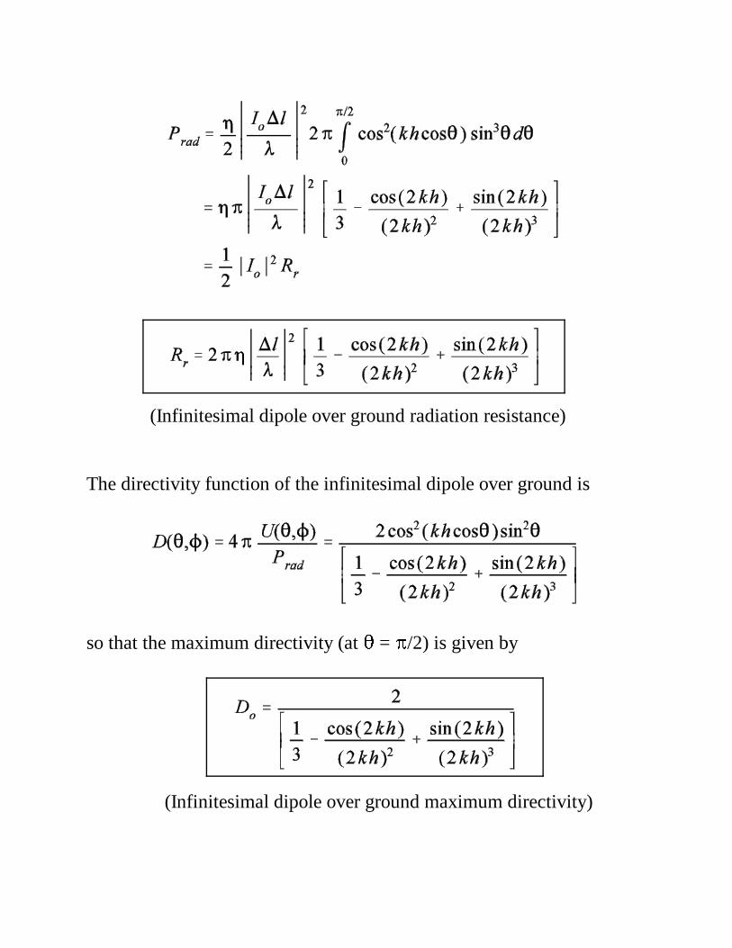
(Infinitesimal dipole over ground radiation resistance)

The directivity function of the infinitesimal dipole over ground is

so that the maximum directivity (at = /2) is given by

(Infinitesimal dipole over ground maximum directivity)

0 0.5 1 1.5 2 2.5 3 3.5 4 4.5 50

0.1

0.2

0.3

0.4

0.5

0.6

0.7

0.8

h/λ

Rr (

Ω)

0 0.5 1 1.5 2 2.5 3 3.5 4 4.5 50

1

2

3

4

5

6

7

8

h/λD

o

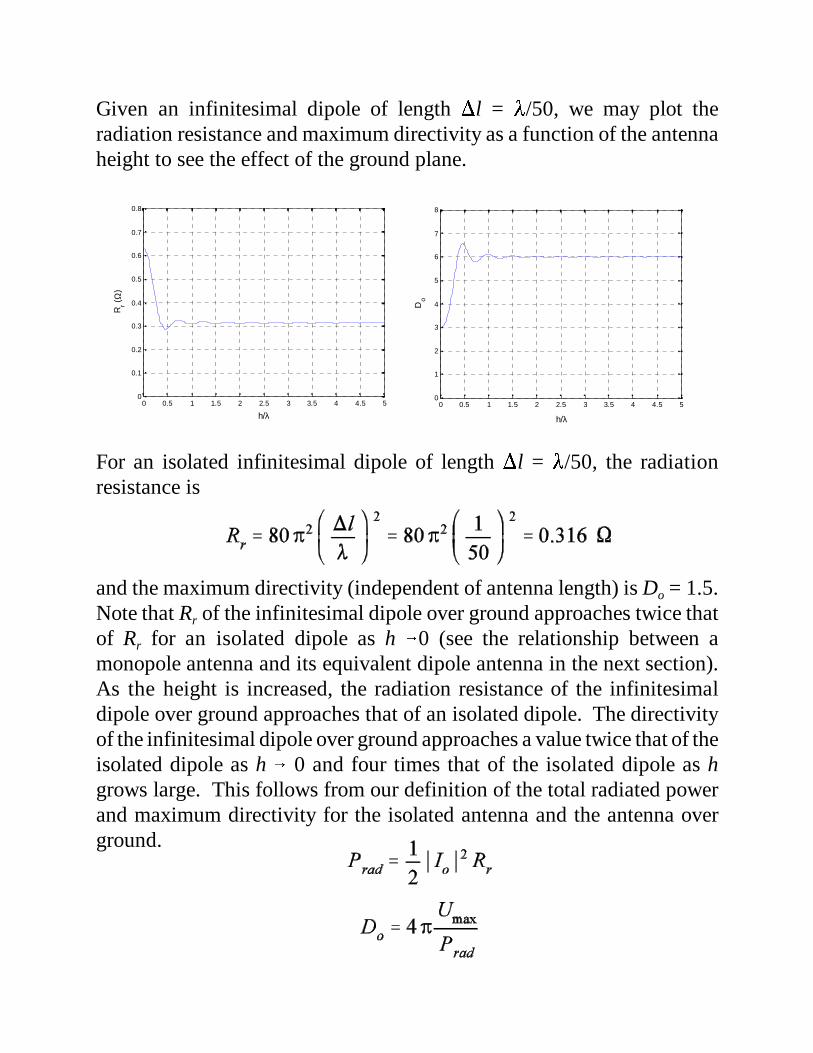
Given an infinitesimal dipole of length l = /50, we may plot theradiation resistance and maximum directivity as a function of the antennaheight to see the effect of the ground plane.

For an isolated infinitesimal dipole of length l = /50, the radiationresistance is

and the maximum directivity (independent of antenna length) is Do = 1.5.Note that Rr of the infinitesimal dipole over ground approaches twice thatof Rr for an isolated dipole as h 0 (see the relationship between amonopole antenna and its equivalent dipole antenna in the next section).As the height is increased, the radiation resistance of the infinitesimaldipole over ground approaches that of an isolated dipole. The directivityof the infinitesimal dipole over ground approaches a value twice that of theisolated dipole as h 0 and four times that of the isolated dipole as hgrows large. This follows from our definition of the total radiated powerand maximum directivity for the isolated antenna and the antenna overground.

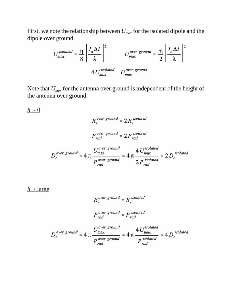
First, we note the relationship between Umax for the isolated dipole and thedipole over ground.

Note that Umax for the antenna over ground is independent of the height ofthe antenna over ground.

h 0

h large

Monopole

Using image theory, the monopole antenna over a PEC ground planemay be shown to be equivalent to a dipole antenna in a homogeneousregion. The equivalent dipole is twice the length of the monopole and isdriven with twice the antenna source voltage. These equivalent antennasgenerate the same fields in the region above the ground plane.

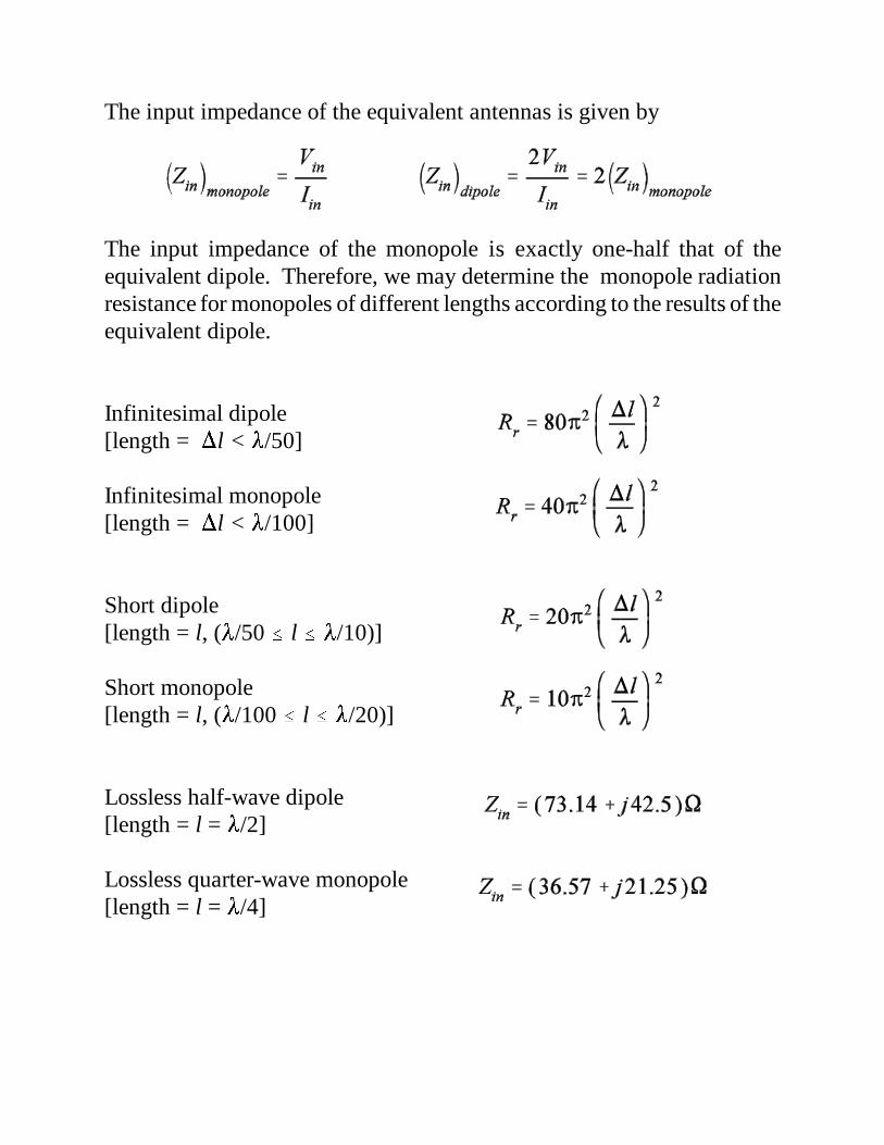
The input impedance of the equivalent antennas is given by

The input impedance of the monopole is exactly one-half that of theequivalent dipole. Therefore, we may determine the monopole radiationresistance for monopoles of different lengths according to the results of theequivalent dipole.

Infinitesimal dipole[length = l < /50]

Infinitesimal monopole[length = l < /100]

Short dipole[length = l, (/50 l /10)]

Short monopole[length = l, (/100 l /20)]

Lossless half-wave dipole[length = l = /2]

Lossless quarter-wave monopole[length = l = /4]

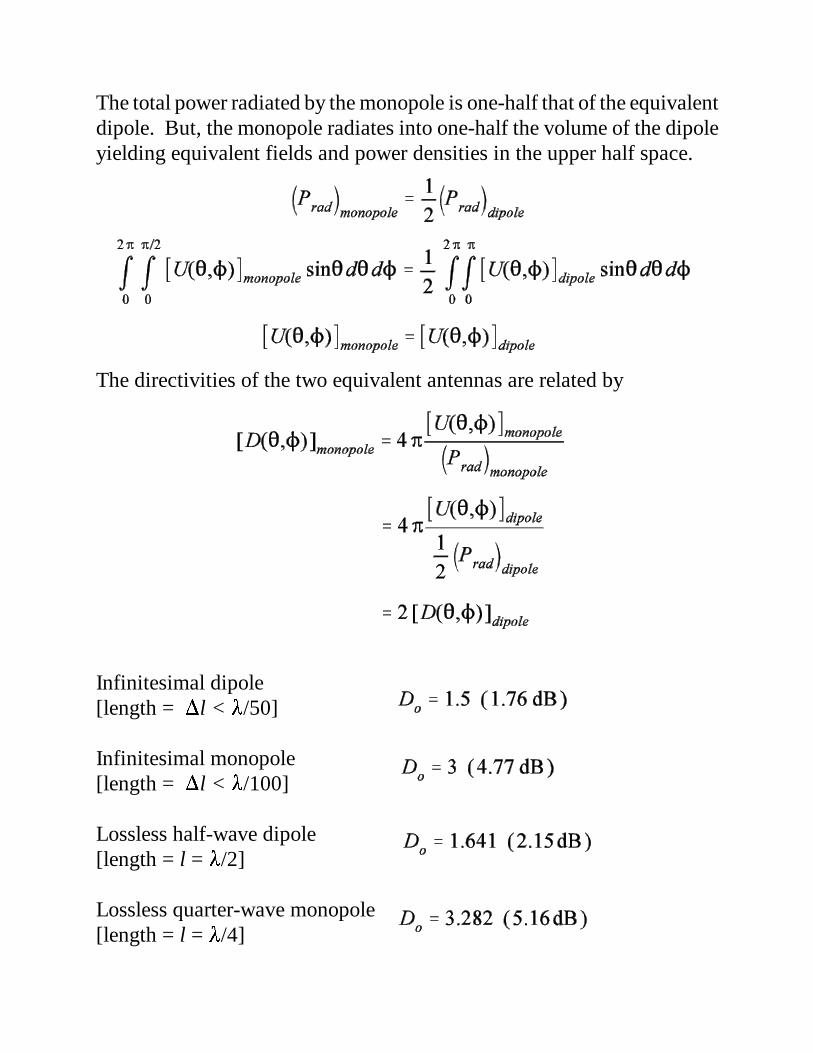
The total power radiated by the monopole is one-half that of the equivalentdipole. But, the monopole radiates into one-half the volume of the dipoleyielding equivalent fields and power densities in the upper half space.

The directivities of the two equivalent antennas are related by

Infinitesimal dipole[length = l < /50]

Infinitesimal monopole[length = l < /100]

Lossless half-wave dipole[length = l = /2]

Lossless quarter-wave monopole[length = l = /4]

Ground Effects on Antennas

At most frequencies, the conductivity of the earth is such that theground may be accurately approximated by a PEC. Given an antennalocated over a PEC ground plane, the radiated fields of the antenna overground can be determined easily using image theory. The fields radiatedby the antenna over a PEC ground excite currents on the surface of theground plane which re-radiate (scatter) the incident waves from theantenna. We may also view the PEC ground plane as a perfect reflector ofthe incident EM waves. The direct wave/reflected wave interpretation ofthe image theory results for the infinitesimal dipole over a PEC ground isshown below.

~~~~~~~~~ ~~~~~~~~~~ direct wave reflected wave

At lower frequencies (approximately 100 MHz and below), theelectric fields associated with the incident wave may penetrate into thelossy ground, exciting currents in the ground which produce ohmic losses.These losses reduce the radiation efficiency of the antenna. They alsoeffect the radiation pattern of the antenna since the incident waves are notperfectly reflected by the ground plane. Image theory can still be used forthe lossy ground case, although the magnitude of the reflected wave mustbe reduced from that found in the PEC ground case. The strength of theimage antenna in the lossy ground case can be found by multiplying thestrength of the image antenna in the PEC ground case by the appropriateplane wave reflection coefficient for the proper polarization (V).

If we plot the radiation pattern of the vertical dipole over ground forcases of a PEC ground and a lossy ground, we find that the elevation planepattern for the lossy ground case is tilted upward such that the radiationmaximum does not occur on the ground plane but at some angle tiltedupward from the ground plane (see Figure 4.28, p. 183). This alignmentof the radiation maximum may or may not cause a problem depending onthe application. However, if both the transmit and receive antennas arelocated close to a lossy ground, then a very inefficient system will result.The antenna over lossy ground can be made to behave more like anantenna over perfect ground by constructing a ground plane beneath theantenna. At low frequencies, a solid conducting sheet is impracticalbecause of its size. However, a system of wires known as a radial groundsystem can significantly enhance the performance of the antenna over lossyground.

Monopole with a radial ground system

The radial wires provide a return path for the currents produced within thelossy ground. Broadcast AM transmitting antennas typically use a radial

ground system with 120 quarter wavelength radial wires (3o spacing).The reflection coefficient scheme can also be applied to horizontal

antennas above a lossy ground plane. The proper reflection coefficientmust be used based on the orientation of the electric field (parallel orperpendicular polarization).

The Effect of Earth Curvature

Antennas on spacecraft and aircraft in flight see the same effect thatantennas located close to the ground experience except that the height ofthe antenna over the conducting ground means that the shape of the ground(curvature of the earth) can have a significant effect on the scattered field.In cases like these, the curvature of the reflecting ground must beaccounted for to yield accurate values for the reflected waves.

Antennas in Wireless Communications

Wire antennas such as dipoles and monopoles are used extensivelyin wireless communications applications. The base stations in wirelesscommunications are most often arrays (Ch. 6) of dipoles. Hand-held unitssuch as cell phones typically use monopoles. Monopoles are simple, small,cheap, efficient, easy to match, omnidirectional (according to theirorientation) and relatively broadband antennas. The equations for theperformance of a monopole antenna presented in this chapter haveassumed that the antenna is located over an infinite ground plane. Themonopole on the hand-held unit is not driven relative to the earth groundbut rather (a.) the conducting case of the unit or (b.) the circuit board of theunit. The resonant frequency and input impedance of the hand-heldmonopole are not greatly different than that of the monopole over a infiniteground plane. The pattern of the hand-held unit monopole is different thanthat of the monopole over an infinite ground plane due to the differentdistribution of currents. Other antennas used on hand-held units are loops(Ch. 5), microstrip (patch) antennas (Ch. 14) and the planar inverted Fantenna (PIFA). In wireless applications, the antenna can be designed to

perform in a typical scenario, but we cannot account for all scatterergeometries which we may encounter (power lines, buildings, etc.). Thus,the scattered signals from nearby conductors can have an adverse effect onthe system performance. The detrimental effect of these unwantedscattered signals is commonly referred to as multipath.

Loop Antennas

Loop antennas have the same desirable characteristics as dipoles andmonopoles in that they are inexpensive and simple to construct. Loopantennas come in a variety of shapes (circular, rectangular, elliptical, etc.)but the fundamental characteristics of the loop antenna radiation pattern(far field) are largely independent of the loop shape.

Just as the electrical length of the dipoles and monopoles effect theefficiency of these antennas, the electrical size of the loop (circumference)determines the efficiency of the loop antenna. Loop antennas are usuallyclassified as either electrically small or electrically large based on thecircumference of the loop.

electrically small loop circumference /10

electrically large loop circumference

The electrically small loop antenna is the dual antenna to theelectrically short dipole antenna when oriented as shown below. That is,the far-field electric field of a small loop antenna is identical to the far-fieldmagnetic field of the short dipole antenna and the far-field magnetic fieldof a small loop antenna is identical to the far-field electric field of the shortdipole antenna.

Given that the radiated fields of the short dipole and small loopantennas are dual quantities, the radiated power for both antennas is thesame and therefore, the radiation patterns are the same. This means thatthe plane of maximum radiation for the loop is in the plane of the loop.When operated as a receiving antenna, we know that the short dipole mustbe oriented such that the electric field is parallel to the wire for maximumresponse. Using the concept of duality, we find that the small loop mustbe oriented such that the magnetic field is perpendicular to the loop formaximum response.

The radiation resistance of the small loop is much smaller than thatof the short dipole. The loss resistance of the small loop antenna isfrequently much larger than the radiation resistance. Therefore, the smallloop antenna is rarely used as a transmit antenna due to its extremely smallradiation efficiency. However, the small loop antenna is acceptable as areceive antenna since signal-to-noise ratio is the driving factor, not antennaefficiency. The fact that a significant portion of the received signal is lostto heat is not of consequence as long as the antenna provides a largeenough signal-to-noise ratio for the given receiver. Small loop antennasare frequently used for receiving applications such as pagers, low-frequency portable radios, and direction finding. Small loops can also beused at higher frequencies as field probes providing a voltage at the loopterminals which is proportional to the field passing through the loop.

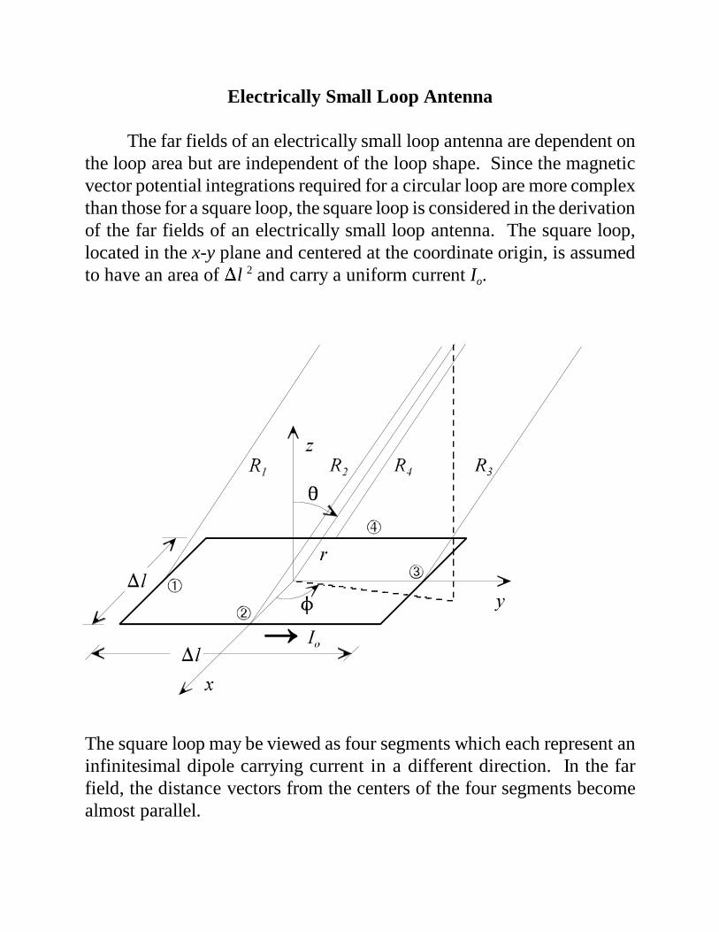
Electrically Small Loop Antenna

The far fields of an electrically small loop antenna are dependent onthe loop area but are independent of the loop shape. Since the magneticvector potential integrations required for a circular loop are more complexthan those for a square loop, the square loop is considered in the derivationof the far fields of an electrically small loop antenna. The square loop,located in the x-y plane and centered at the coordinate origin, is assumedto have an area of l 2 and carry a uniform current Io.

The square loop may be viewed as four segments which each represent aninfinitesimal dipole carrying current in a different direction. In the farfield, the distance vectors from the centers of the four segments becomealmost parallel.

As always in far field expressions, the above approximations are used inthe phase terms of the magnetic vector potential, but we may assume thatR1 R2 R3 R4 r for the magnitude terms. The far field magneticvector potential of a z-directed infinitesimal dipole centered at the originis

The individual far field magnetic vector potential contributions due to thefour segments of the current loop are

Combining the x-directed and y-directed terms yields

For an electrically small loop (l << ), the arguments of the sinefunctions above are very small and may be approximated according to

which gives

The overall vector potential becomes

where S = l2 = loop area. The bracketed term above is the sphericalcoordinate unit vector a.

Electrically small current loop far field magnetic vector potential

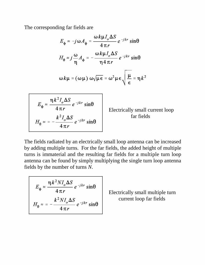
The corresponding far fields are

Electrically small current loop far fields

The fields radiated by an electrically small loop antenna can be increasedby adding multiple turns. For the far fields, the added height of multipleturns is immaterial and the resulting far fields for a multiple turn loopantenna can be found by simply multiplying the single turn loop antennafields by the number of turns N.

Electrically small multiple turn current loop far fields

Dual and Equivalent Sources(Electric and Magnetic Dipoles and Loops)

If we compare the far fields of the infinitesimal dipole and theelectrically small current loop with electric and magnetic currents, we findpairs of equivalent sources and dual sources.

Infinitesimal electric dipole Small electric current loop

Using duality, we may determine the far fields of the correspondingmagnetic geometries.

Electric source Magnetic source

Infinitesimal magnetic dipole Small magnetic current loop

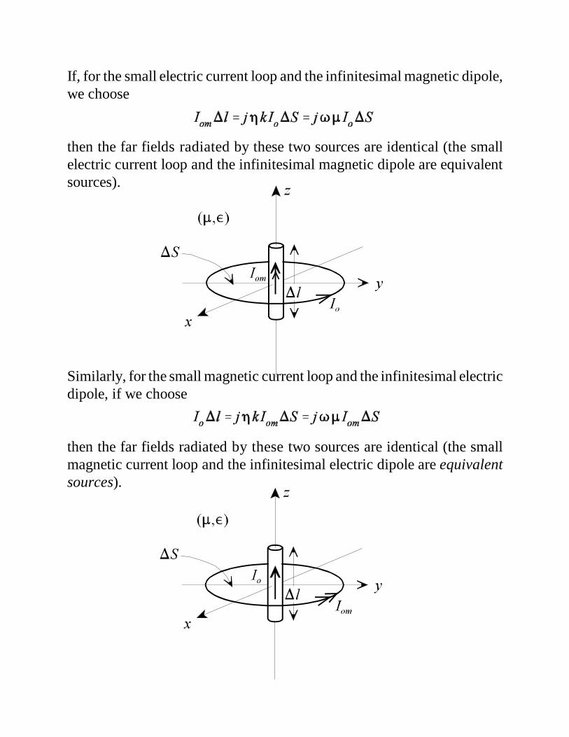
If, for the small electric current loop and the infinitesimal magnetic dipole,we choose

then the far fields radiated by these two sources are identical (the smallelectric current loop and the infinitesimal magnetic dipole are equivalentsources).

Similarly, for the small magnetic current loop and the infinitesimal electricdipole, if we choose

then the far fields radiated by these two sources are identical (the smallmagnetic current loop and the infinitesimal electric dipole are equivalentsources).

The infinitesimal electric and magnetic dipoles are defined as dual sourcessince the magnetic field of one is identical to the electric field of the otherwhen the currents and dimensions are chosen appropriately. Likewise, thesmall electric and magnetic current loops are dual sources.

We also find from this discussion of dual and equivalent sources thatthe polarization of the far fields for the dual sources are orthogonal. In theplane of maximum radiation (x-y plane), the four sources have thefollowing far field polarizations

infinitesimal electric dipole vertical polarization

infinitesimal magnetic dipole horizontal polarization

small electric current loop horizontal polarization

small magnetic current loop vertical polarization

Loop Antenna Characteristics

The time-average Poynting vector in the far field of the multiple-turnelectrically small loop is

The radiation intensity function is

Loop antenna radiation intensity function

The maximum value of the radiation intensity function is

The radiated power is

Loop antenna radiated power

The radiation resistance of the loop antenna is found from the radiatedpower.

Loop antenna in airradiation resistance

The directivity of the loop antenna is defined by

Loop antenna

directivity function

Given the same directivity function as the infinitesimal dipole, the loopantenna has the same maximum directivity, effective aperture and beamsolid angle as the infinitesimal dipole.

Loop antenna

maximum directivity, effective aperture, and beam solid angle

Loop-stick antenna

If we compare the radiation resistances of the electrically short dipoleand the electrically small loop (both antennas in air), we find that theradiation resistance of the small loop decreases much faster than that of theshort dipole with decreasing frequency since

Rr (short dipole) ~ 2

Rr (small loop) ~ 4

The radiation resistance of the small loop can be increased significantly byadding multiple turns (Rr ~ N2). However, the addition of more conductorlength also increases the antenna loss resistance which reduces the overallantenna efficiency. To increase the radiation resistance withoutsignificantly reducing the antenna efficiency, the number of turns can bedecreased when a ferrite material is used as the core of the winding. Thegeneral radiation resistance formula for a smallloop with any material as its core is

A multiturn loop which is wound on a linear ferritecore is commonly referred to as a loop-stickantenna. The loop-stick antenna is commonly usedas a low-frequency receiving antenna.

Impedance of Electrically Small Antennas

The current density was assumed to be uniform on the electricallysmall current loop for our far field calculations. For a circular loop, theassumption of uniform current is accurate up to a loop circumference ofabout 0.2.

b = loop radius

a = wire radius

The restriction on the size of the constant current loop in terms of the loopradius is

The electrically small current loop was found to be a dual source tothe infinitesimal dipole. If we investigate the reactance of these dualelectrically small antennas, we find that the dipole is capacitive while theloop is inductive. The exact reactance of the current loop is dependent onthe shape of the loop. Approximate formulas for the reactance are givenbelow for a short dipole and an electrically small circular current loop.

Infinitesimal Dipole (length = l, wire radius = a)

Electrically Small Circular Current Loop (loop radius = b, wire radius = a)

Example (Impedances of electrically small antennas)

Determine the total impedance and radiation efficiency of thefollowing electrically small antennas operating at 1, 10 and 100 MHz. Both antennas are constructed using #10 AWG copper wire (a = 2.59 mm, = 5.8 × 107 /m).

Infinitesimal Dipole

f (MHz) l Rr RL ecd jXA

1 0.0002 31.6 0.962 m 3.18 % 204 k

10 0.002 3.16 m 3.04 m 51.0 % 20.4 k

100 0.02 0.316 9.62 m 97.0 % 2.04 k

Small Loop

f (MHz) b Rr RL ecd jXA

1 0.00032 3.09 n 9.57 m 3.2×10-5 % 2.76

10 0.0032 30.9 30.3 m 0.102 % 27.6

100 0.032 0.309 95.7 m 76.4% 276

Antenna Arrays

Antennas with a given radiation pattern may be arranged in a pattern(line, circle, plane, etc.) to yield a different radiation pattern.

Antenna array - a configuration of multiple antennas (elements)arranged to achieve a given radiation pattern.

Linear array - antenna elements arranged along a straight line.

Circular array - antenna elements arranged around a circularring.

Planar array - antenna elements arranged over some planarsurface (example - rectangular array).

Conformal array - antenna elements arranged to conform tosome non-planar surface (such as an aircraft skin).

There are several array design variables which can be changed to achievethe overall array pattern design.

Array Design Variables

1. General array shape (linear, circular, planar, etc.).2. Element spacing.3. Element excitation amplitude.4. Element excitation phase.5. Patterns of array elements.

Phased array - an array of identical elements which achieves a givenpattern through the control of the element excitation phasing.Phased arrays can be used to steer the main beam of theantenna without physically moving the antenna.

Given an antenna array of identical elements, the radiation pattern of theantenna array may be found according to the pattern multiplicationtheorem.

Pattern multiplication theorem

Array element pattern - the pattern of the individual array element.Array factor - a function dependent only on the geometry of the array

and the excitation (amplitude, phase) of the elements.

Example (Pattern multiplication - infinitesimal dipole over ground)

The far field of this two element array was found using image theory to be

element pattern array factor

N-Element Linear Array

The array factor AF is independent of the antenna type assuming allof the elements are identical. Thus, isotropic radiators may be utilized inthe derivation of the array factor to simplify the algebra. The field of anisotropic radiator located at the origin may be written as (assuming -polarization)

We assume that the elements of the array are uniformly-spaced with aseparation distance d.

In the far field of the array

The current magnitudes the array elements are assumed to be equal and thecurrent on the array element located at the origin is used as the phasereference (zero phase).

The far fields of the individual array elements are

The overall array far field is found using superposition.

(Array factor for a uniformly-spaced N-element linear array)

Uniform N-Element Linear Array(uniform spacing, uniform amplitude, linear phase progression)

A uniform array is defined by uniformly-spaced identical elementsof equal magnitude with a linearly progressive phase from element toelement.

Inserting this linear phase progression into the formula for the general N-element array gives

The function is defined as the array phase function and is a function ofthe element spacing, phase shift, frequency and elevation angle. If thearray factor is multiplied by e j, the result is

Subtracting the array factor from the equation above gives

The complex exponential term in the last expression of the above equationrepresents the phase shift of the array phase center relative to the origin.If the position of the array is shifted so that the center of the array islocated at the origin, this phase term goes away.

The array factor then becomes

Below are plots of the array factor AF vs. the array phase function as thenumber of elements in the array is increased. Note that these are notplots of AF vs. the elevation angle .

Some general characteristics of the array factor AF with respect to :(1) [AF ]max = N at = 0 (main lobe).(2) Total number of lobes = N1 (one main lobe, N2 sidelobes).(3) Main lobe width = 4/N, minor lobe width = 2/N

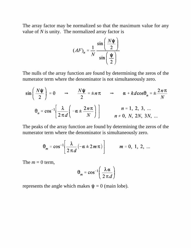
The array factor may be normalized so that the maximum value for anyvalue of N is unity. The normalized array factor is

The nulls of the array function are found by determining the zeros of thenumerator term where the denominator is not simultaneously zero.

The peaks of the array function are found by determining the zeros of thenumerator term where the denominator is simultaneously zero.

The m = 0 term,

represents the angle which makes = 0 (main lobe).

Broadside and End-fire Arrays

The phasing of the uniform linear array elements may be chosen suchthat the main lobe of the array pattern lies along the array axis (end-firearray) or normal to the array axis (broadside array).

End-fire array main lobe at = 0o or = 180o

Broadside array main lobe at = 90o

The maximum of the array factor occurs when the array phase function iszero.

For a broadside array, in order for the above equation to be satisfied with = 90o, the phase angle must be zero. In other words, all elements of thearray must be driven with the same phase. With = 0o, the normalizedarray factor reduces to

Normalized array function Broadside array, = 0o

Consider a 5-element broadside array ( = 0o) as the element spacing isvaried. In general, as the element spacing is increased, the main lobebeamwidth is decreased. However, grating lobes (maxima in directionsother than the main lobe direction) are introduced when the elementspacing is greater than or equal to one wavelength. If the array patterndesign requires that no grating lobes be present, then the array elementspacing should be chosen to be less than one wavelength.

If we consider the broadside array factor as a function of the number ofarray elements, we find that, in general, the main beam is sharpened as thenumber of elements increases. Below are plots of AF for a broadside array( = 0o) with elements separated by d = 0.25 for N = 2, 5, 10 and 20.

Using the pattern multiplication theorem, the overall array pattern isobtained by multiplying the element pattern by the array factor. As anexample, consider an broadside array ( = 0o) of seven short verticaldipoles spaced 0.5 apart along the z-axis.

The normalized element field pattern for the infinitesimal dipole is

The array factor for the seven element array is

The overall normalized array pattern is

0.2

0.4

0.6

0.8

1

30

210

60

240

90

270

120

300

150

330

180 0

element pattern

0.5

1

30

210

60

240

90

270

120

300

150

330

180 0

array factor

If we consider the same array with horizontal (x-directed) short dipoles, theresulting normalized element field pattern is

Since the element pattern depends on the angle , we must choose a valueof to plot the pattern. If we choose = 0o, the element pattern becomes

and the array pattern is given by

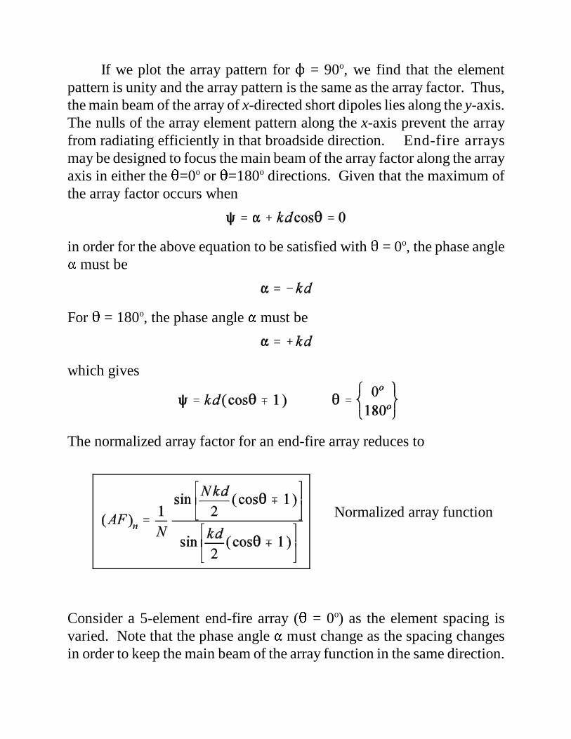
If we plot the array pattern for = 90o, we find that the elementpattern is unity and the array pattern is the same as the array factor. Thus,the main beam of the array of x-directed short dipoles lies along the y-axis.The nulls of the array element pattern along the x-axis prevent the arrayfrom radiating efficiently in that broadside direction. End-fire arraysmay be designed to focus the main beam of the array factor along the arrayaxis in either the =0o or =180o directions. Given that the maximum ofthe array factor occurs when

in order for the above equation to be satisfied with = 0o, the phase angle must be

For = 180o, the phase angle must be

which gives

The normalized array factor for an end-fire array reduces to

Normalized array function

Consider a 5-element end-fire array ( = 0o) as the element spacing isvaried. Note that the phase angle must change as the spacing changesin order to keep the main beam of the array function in the same direction.

If the corresponding positive phase angles are chosen, the array factor plotsare mirror images of the above plots (about = 90o ). Note that the end-fire array grating lobes are introduced for element spacings of d 0.5.

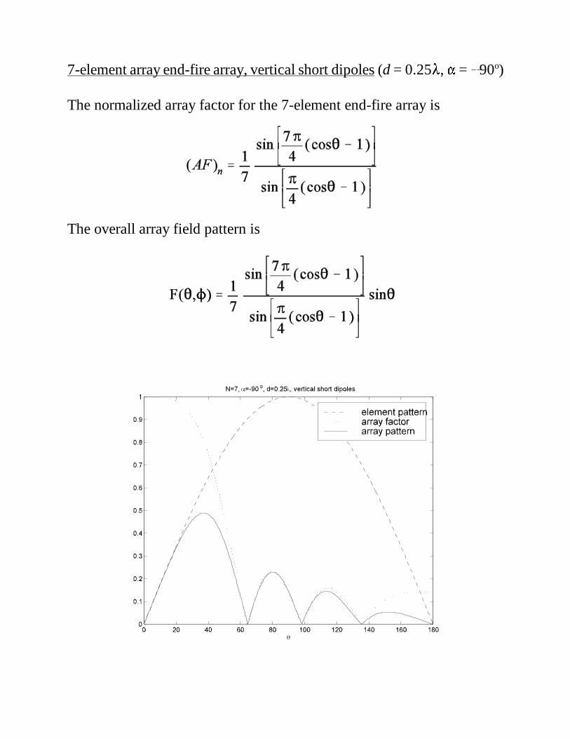
7-element array end-fire array, vertical short dipoles (d = 0.25, = 90o)

The normalized array factor for the 7-element end-fire array is

The overall array field pattern is

0.2

0.4

0.6

0.8

1

30

210

60

240

90

270

120

300

150

330

180 0

element pattern

0.2

0.4

0.6

0.8

1

30

210

60

240

90

270

120

300

150

330

180 0

array factor

0.1

0.2

0.3

0.4

0.5

30

210

60

240

90

270

120

300

150

330

180 0

array pattern

7-element end-fire array, x-directed horizontal short dipoles(d = 0.25, = 90o)

The overall array pattern in the = 0o plane is

0.2

0.4

0.6

0.8

1

30

210

60

240

90

270

120

300

150

330

180 0

element pattern

0.2

0.4

0.6

0.8

1

30

210

60

240

90

270

120

300

150

330

180 0

array factor

0.2

0.4

0.6

0.8

1

30

210

60

240

90

270

120

300

150

330

180 0

array pattern

Hansen-Woodyard End-fire Array

The Hansen-Woodyard end-fire array is a special array designed formaximum directivity.

Ordinary end-fire array = ±kd

Hansen-Woodyard end-fire array = ± (kd + )

In order to increase the directivity in a closely-spaced electrically long end-fire array, Hansen and Woodyard analyzed the patterns and found that aadditional phase shift of

increased the directivity of the array over that of the ordinary end-fire arraygiven an element spacing of

For very long arrays (N - large), the element spacing in the Hansen-Woodyard end-fire array approaches one-quarter wavelength. The Hansen-Woodyard design shown here does not necessarily produce the maximumdirectivity for a given linear array but does produce a directivity larger thanthat of the ordinary end-fire array [by a factor of approximately 1.79 (2.5dB)]. The Hansen-Woodyard end-fire array design can be summarized as

where the upper sign produces a maximum in the = 0o direction and thelower sign produces a maximum in the = 180o direction. The Hansen-Woodyard end-fire design increases the directivity of the array at theexpense of higher sidelobe levels.

Non-Uniformly Excited, Equally-Spaced Arrays

Given a two element array with equal current amplitudes andspacing, the array factor is

For a broadside array ( = 0o) with element spacing d less than one-halfwavelength, the array factor has no sidelobes. An array formed by takingthe product of two arrays of this type gives

This array factor, being the square of an array factor with no sidelobes, alsohas no sidelobes. Mathematically, the array factor above represents a 3-element equally-spaced array driven by current amplitudes with ratios of1:2:1. In a similar fashion, equivalent arrays with more elements may beformed.

The current coefficients of the resulting N-element array take the form ofa binomial series. The array is known as a binomial array.

Binomial array

The excitation coefficients for the binomial array are given by Pascal’striangle.

The binomial array has the special property that the array factor has nosidelobes for element spacings of /2 or less. Sidelobes are introduced forelement spacings larger than /2.

N = 5, d = 0.5 N = 10, d = 0.5

Array Factor - Uniform Spacing, Nonuniform Amplitude

Consider an array of isotropic elements positioned symmetricallyalong the z-axis (total number of elements = P). The array factor for thisarray will be determined assuming that all elements are excited with thesame current phase ( = 0o for simplicity) but nonuniform currentamplitudes. The amplitude distribution assumed to be symmetric about theorigin.

P = 2M + 1 (Odd) P = 2M (Even)

P = 2M + 1 (Odd) P = 2M (Even)

P = 2M + 1 (Odd)

where

P = 2M (Even)

Note that the array factors are coefficients multiplied by cosines witharguments that are integer multiples of u. Using trigonometric identities,these cosine functions can be written as powers of u.

Through the transformation of x = cos u, the terms may be written as a setof polynomials [Chebyshev polynomials - Tn(x)].

Using properties of the Chebyshev polynomials, we may design arrays withspecific sidelobe characteristics. Namely, we may design arrays with allsidelobes at some prescribed level.

Chebyshev Polynomials

Properties of Chebyshev Polynomials

1. Even ordered Chebyshev polynomials are even functions.2. Odd ordered Chebyshev polynomials are odd functions.3. The magnitude of any Chebyshev polynomial is unity or less in the

range of 1 x 1.4. Tn (1) = 1 for all Chebyshev polynomials.5. All zeros (roots) of the Chebshev polynomials lie within the range of

1 x 1.

Using the properties of Chebyshev polynomials, we may design arrays withall sidelobes at a prescribed level below the main beam (Dolph-Chebyshevarray). The order of the Chebyshev polynomial should be one less than thetotal number of elements in the array (P1).

Dolph-Chebyshev Array Design Procedure

(1.) Select the appropriate AF for the total number of elements (P).

(2.) Replace each cos(mu) term in the array factor by its expansion interms of powers of cos(u).

(3.) For the required main lobe to side lobe ratio (Ro), find xo such that

(4.) Substitute cos(u) = x/xo into the array factor of step 2. Thissubstitution normalizes the array factor sidelobes to a peak of unity.

(5.) Equate the array factor of step 4 to TP-1(x) and determine the arraycoefficients.

Example

Design a 5-element Dolph-Chebyshev array with d = 0.5 andsidelobes which are 20 dB below the main beam.

(1.) P = 5, M = 2

(2.)

(3.)

(4.)

(5.) Equate coefficients and solve for a1, a2, and a3.

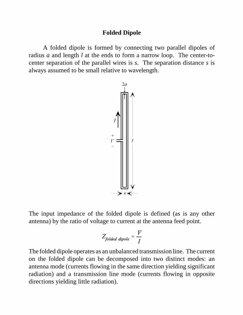
Folded Dipole

A folded dipole is formed by connecting two parallel dipoles ofradius a and length l at the ends to form a narrow loop. The center-to-center separation of the parallel wires is s. The separation distance s isalways assumed to be small relative to wavelength.

The input impedance of the folded dipole is defined (as is any otherantenna) by the ratio of voltage to current at the antenna feed point.

The folded dipole operates as an unbalanced transmission line. The currenton the folded dipole can be decomposed into two distinct modes: anantenna mode (currents flowing in the same direction yielding significantradiation) and a transmission line mode (currents flowing in oppositedirections yielding little radiation).

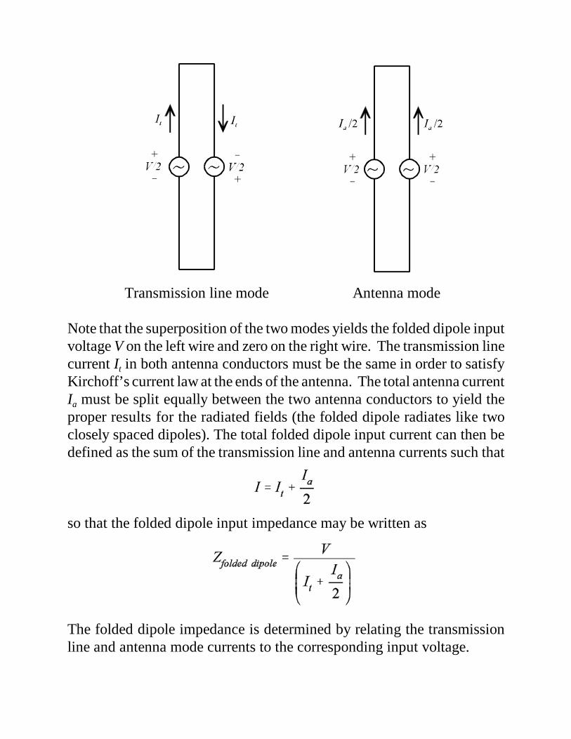
Transmission line mode Antenna mode

Note that the superposition of the two modes yields the folded dipole inputvoltage V on the left wire and zero on the right wire. The transmission linecurrent It in both antenna conductors must be the same in order to satisfyKirchoff’s current law at the ends of the antenna. The total antenna currentIa must be split equally between the two antenna conductors to yield theproper results for the radiated fields (the folded dipole radiates like twoclosely spaced dipoles). The total folded dipole input current can then bedefined as the sum of the transmission line and antenna currents such that

so that the folded dipole input impedance may be written as

The folded dipole impedance is determined by relating the transmissionline and antenna mode currents to the corresponding input voltage.

We may insert an equivalent set of voltagesources into the transmission line modeproblem in order to view the folded dipole as aset of two shorted transmission lines of lengthl/2. Note that both of the shorted transmissionlines are driven with a source voltage of V/2across its input terminals. The voltage andcurrent for the transmission lines are related by

where Zt is the input impedance of a shortedtwo-wire line of length l/2 with wire of radii awith a center-to-center spacing of s. Thegeneral equation for the input impedance of atransmission line of characteristic impedance Zo

and length l terminated with an load impedanceZL is

For the shorted line, ZL = 0 and the length isl/2 so that

The characteristic impedance of the two wireline transmission line is

The folded dipole antenna current can be related to an equivalentdipole (treating the parallel currents as coincident for far field purposes)by

where Zd is the input impedance of a dipole of length l and equivalentradius ae. The equivalent radius is necessary because of the closeproximity of the two wires (capacitance) which alters the currentdistribution from that seen on an isolated dipole. The equivalent radius isgiven by

The impedance Zd is given by

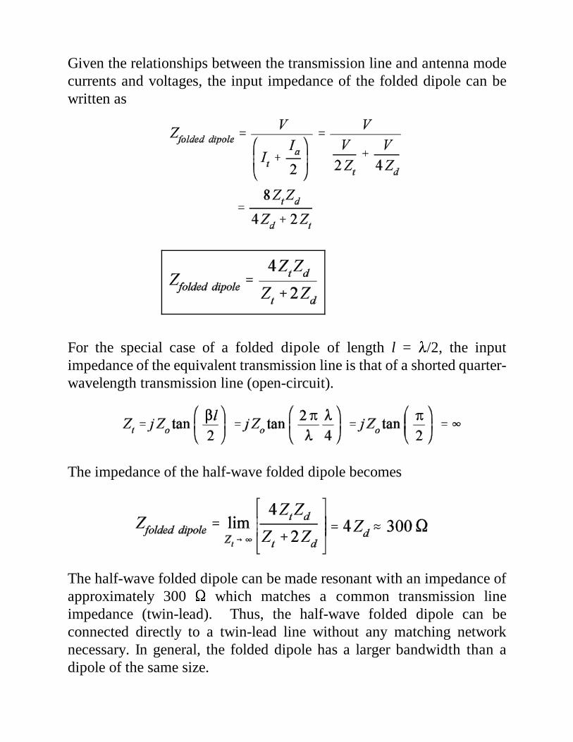
Given the relationships between the transmission line and antenna modecurrents and voltages, the input impedance of the folded dipole can bewritten as

For the special case of a folded dipole of length l = /2, the inputimpedance of the equivalent transmission line is that of a shorted quarter-wavelength transmission line (open-circuit).

The impedance of the half-wave folded dipole becomes

The half-wave folded dipole can be made resonant with an impedance ofapproximately 300 which matches a common transmission lineimpedance (twin-lead). Thus, the half-wave folded dipole can beconnected directly to a twin-lead line without any matching networknecessary. In general, the folded dipole has a larger bandwidth than adipole of the same size.

Traveling Wave Antennas

Antennas with open-ended wires where the current must go to zero(dipoles, monopoles, etc.) can be characterized as standing wave antennasor resonant antennas. The current on these antennas can be written as asum of waves traveling in opposite directions (waves which travel towardthe end of the wire and are reflected in the opposite direction). Forexample, the current on a dipole of length l is given by

The current on the upper arm of the dipole can be written as

+z directed z directed wave wave

Traveling wave antennas are characterized by matched terminations (notopen circuits) so that the current is defined in terms of waves traveling inonly one direction (a complex exponential as opposed to a sine or cosine).

A traveling wave antenna can be formed by a single wire transmission line(single wire over ground) which is terminated with a matched load (noreflection). Typically, the length of the transmission line is severalwavelengths.

The antenna shown above is commonly called a Beverage or waveantenna. This antenna can be analyzed as a rectangular loop, according toimage theory. However, the effects of an imperfect ground may besignificant and can be included using the reflection coefficient approach.The contribution to the far fields due to the vertical conductors is typicallyneglected since it is small if l >> h. Note that the antenna does not radiateefficiently if the height h is small relative to wavelength. In an alternativetechnique of analyzing this antenna, the far field produced by a longisolated wire of length l can be determined and the overall far field foundusing the 2 element array factor.

Traveling wave antennas are commonly formed using wire segmentswith different geometries. Therefore, the antenna far field can be obtainedby superposition using the far fields of the individual segments. Thus, theradiation characteristics of a long straight segment of wire carrying atraveling wave type of current are necessary to analyze the typical travelingwave antenna.

Consider a segment of a traveling wave antenna (an electrically longwire of length l lying along the z-axis) as shown below. A traveling wavecurrent flows in the z-direction.

- attenuation constant

- phase constant

If the losses for the antenna are negligible (ohmic loss in the conductors,loss due to imperfect ground, etc.), then the current can be written as

The far field vector potential is

If we let , then

The far fields in terms of the far field vector potential are

(Far-field of a traveling wave segment)

We know that the phase constant of a transmission line wave (guidedwave) can be very different than that of an unbounded medium (unguidedwave). However, for a traveling wave antenna, the electrical height of theconductor above ground is typically large and the phase constantapproaches that of an unbounded medium (k). If we assume that the phaseconstant of the traveling wave antenna is the same as an unboundedmedium ( = k), then

Given the far field of the traveling wave segment, we may determine thetime-average radiated power density according to the definition of thePoynting vector such that

The total power radiated by the traveling wave segment is found byintegrating the Poynting vector.

and the radiation resistance is

The radiation resistance of the ideal traveling wave antenna (VSWR = 1)is purely real just as the input impedance of a matched transmission lineis purely real. Below is a plot of the radiation resistance of the travelingwave segment as a function of segment length.

The radiation resistance of the traveling wave antenna is much moreuniform than that seen in resonant antennas. Thus, the traveling waveantenna is classified as a broadband antenna.

The pattern function of the traveling wave antenna segment is givenby

The normalized pattern function can be written as

The normalized pattern function of the traveling wave segment is shownbelow for segment lengths of 5, 10, 15 and 20.

l = 5 l = 10

l = 15 l = 20

As the electrical length of the traveling wave segment increases, themain beam becomes slightly sharper while the angle of the main beammoves slightly toward the axis of the antenna.

Note that the pattern function of the traveling wave segment alwayshas a null at = 0o. Also note that with l >> , the sine function in thenormalized pattern function varies much more rapidly (more peaks andnulls) than the cotangent function. The approximate angle of the main lobefor the traveling wave segment is found by determining the first peak of thesine function in the normalized pattern function.

The values of m which yield 0om180o (visible region) are negative

values of m. The smallest value of m in the visible region defines thelocation of main beam (m = 1)

If we also account for the cotangent function in the determination of themain beam angle, we find

The directivity of the traveling wave segment is

The maximum directivity can be approximated by

where the sine term in the numerator of the directivity function is assumedto be unity at the main beam.

Traveling Wave Antenna Terminations

Given a traveling wave antenna segment located horizontally abovea ground plane, the termination RL required to match the uniformtransmission line formed by the cylindrical conductor over ground (radius= a, height over ground = s/2) is the characteristic impedance of thecorresponding one-wire transmission line. If the conductor height abovethe ground plane varies with position, the conductor and the ground planeform a non-uniform transmission line. The characteristic impedance of anon-uniform transmission line is a function of position. In either case,image theory may be employed to determine the overall performancecharacteristics of the traveling wave antenna.

Two-wire transmission line

If s >> a, then

In air,

One-wire transmission line

If s >> a, then

In air,

Vee Traveling Wave Antenna

The main beam of a single electrically long wire guiding waves inone direction (traveling wave segment) was found to be inclined at anangle relative to the axis of the wire. Traveling wave antennas are typicallyformed by multiple traveling wave segments. These traveling wavesegments can be oriented such that the main beams of the component wirescombine to enhance the directivity of the overall antenna. A vee travelingwave antenna is formed by connecting two matched traveling wavesegments to the end of a transmission line feed at an angle of 2o relativeto each other.

The beam angle of a traveling wave segment relative to the axis of the wire(max) has been shown to be dependent on the length of the wire. Given thelength of the wires in the vee traveling wave antenna, the angle 2o may bechosen such that the main beams of the two tilted wires combine to forman antenna with increased directivity over that of a single wire.

A complete analysis which takes into account the spatial separation effectsof the antenna arms (the two wires are not co-located) reveals that bychoosing o 0.8 max, the total directivity of the vee traveling waveantenna is approximately twice that of a single conductor. Note that theoverall pattern of the vee antenna is essentially unidirectional givenmatched conductors.

If, on the other hand, the conductors of the vee traveling waveantenna are resonant conductors (vee dipole antenna), there are reflectedwaves which produce significant beams in the opposite direction. Thus,traveling wave antennas, in general, have the advantage of essentiallyunidirectional patterns when compared to the patterns of most resonantantennas.

Rhombic Antenna

A rhombic antenna is formed by connecting two vee traveling waveantennas at their open ends. The antenna feed is located at one end of therhombus and a matched termination is located at the opposite end. As withall traveling wave antennas, we assume that the reflections from the loadare negligible. Typically, all four conductors of the rhombic antenna areassumed to be the same length. Note that the rhombic antenna is anexample of a non-uniform transmission line.

A rhombic antenna can also be constructed using an inverted vee antennaover a ground plane. The termination resistance is one-half that requiredfor the isolated rhombic antenna.

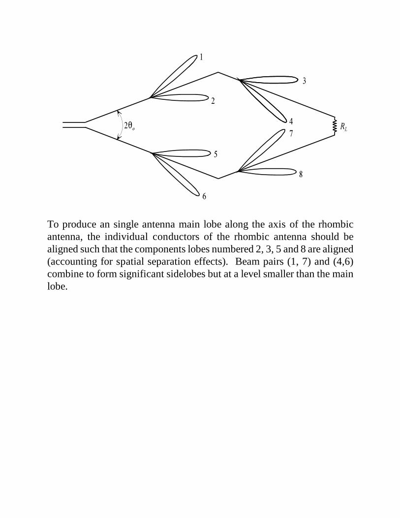
To produce an single antenna main lobe along the axis of the rhombicantenna, the individual conductors of the rhombic antenna should bealigned such that the components lobes numbered 2, 3, 5 and 8 are aligned(accounting for spatial separation effects). Beam pairs (1, 7) and (4,6)combine to form significant sidelobes but at a level smaller than the mainlobe.

Yagi-Uda Array

In the previous examples of array design, all of the elements in thearray were assumed to be driven with some source. A Yagi-Uda array isan example of a parasitic array. Any element in an array which is notconnected to the source (in the case of a transmitting antenna) or thereceiver (in the case of a receiving antenna) is defined as a parasiticelement. A parasitic array is any array which employs parasitic elements.The general form of the N-element Yagi-Uda array is shown below.

Driven element - usually a resonant dipole or folded dipole.

Reflector - slightly longer than the driven element so that it isinductive (its current lags that of the driven element).

Director - slightly shorter than the driven element so that it iscapacitive (its current leads that of the driven element).

Yagi-Uda Array Advantages

Lightweight Low cost Simple construction Unidirectional beam (front-to-back ratio) Increased directivity over other simple wire antennas Practical for use at HF (3-30 MHz), VHF (30-300 MHz), and

UHF (300 MHz - 3 GHz)

Typical Yagi-Uda Array Parameters

Driven element half-wave resonant dipole or folded dipole,(Length = 0.45 to 0.49, dependent on radius), folded dipolesare employed as driven elements to increase the array inputimpedance.

Director Length = 0.4 to 0.45 (approximately 10 to 20 % shorterthan the driven element), not necessarily uniform.

Reflector Length 0.5 (approximately 5 to 10 % longer than thedriven element).

Director spacing approximately 0.2 to 0.4, not necessarilyuniform.

Reflector spacing 0.1 to 0.25

Example (Yagi-Uda Array)

Given a simple 3-element Yagi-Uda array (one reflector - length =0.5, one director - length = 0.45, driven element - length = 0.475)where all the elements are the same radius (a = 0.005). For sR = sD =0.1, 0.2 and 0.3, determine the E-plane and H-plane patterns, the 3dBbeamwidths in the E- and H-planes, the front-to-back ratios (dB) in the E-and H-planes, and the maximum directivity (dB). Also, plot the currentsalong the elements in each case. Use the FORTRAN program providedwith the textbook (yagi-uda.for). Use 8 modes per element in the methodof moments solution.

The individual element currents given as outputs of the FORTRAN codeare all normalized to the current at the feed point of the antenna.

sR = sD = 0.1

sR = sD = 0.2

sR = sD = 0.3

sR = sD = 0.1

3-dB beamwidth E-Plane = 62.71o

3-dB beamwidth H-Plane = 86.15o

Front-to-back ratio E-Plane = 15.8606 dB

Front-to-back-ratio H-Plane = 15.8558 dB

Maximum directivity = 7.784 dB

sR = sD = 0.2

3-dB beamwidth E-Plane = 55.84o

3-dB beamwidth H-Plane = 69.50o

Front-to-back ratio E-Plane = 9.2044 dB

Front-to-back-ratio H-Plane = 9.1993 dB

Maximum directivity = 9.094 dB

sR = sD = 0.3

3-dB beamwidth E-Plane = 51.89o

3-dB beamwidth H-Plane = 61.71o

Front-to-back ratio E-Plane = 5.4930 dB

Front-to-back-ratio H-Plane = 5.4883 dB

Maximum directivity = 8.973 dB

Example

15-element Yagi-Uda Array (13 directors, 1 reflector, 1 driven element)

reflector length = 0.5 reflector spacing = 0.25director lengths = 0.406 director spacing = 0.34driven element length = 0.47 conductor radii = 0.003

3-dB beamwidth E-Plane = 26.79o

3-dB beamwidth H-Plane = 27.74o

Front-to-back ratio E-Plane = 36.4422 dB

Front-to-back-ratio H-Plane = 36.3741 dB

Maximum directivity = 14.700 dB

(1)

Log-Periodic Antenna

A log-periodic antenna is classified as a frequency-independentantenna. No antenna is truly frequency-independent but antennas capableof bandwidth ratios of 10:1 ( fmax : fmin ) or more are normally classified asfrequency-independent.

The elements of the log periodic dipole are bounded by a wedge ofangle 2. The element spacing is defined in terms of a scale factor suchthat

(2)

(3)

(4)

(5)

(6)

where < 1. Using similar triangles, the angle is related to the elementlengths and positions according to

or

Combining equations (1) and (3), we find that the ratio of adjacent elementlengths and the ratio of adjacent element positions are both equal to thescale factor.

The spacing factor of the log periodic dipole is defined by

where dn is the distance from element n to element n+1 .

From (2), we may write

Inserting (6) into (5) yields

(7)

(8)

(9)

(10)

(11)

Combining equation (3) with equation (7) gives

or

According to equation (8), the ratio of element spacing to element lengthremains constant for all of the elements in the array.

Combining equations (3) and (10) shows that z-coordinates, the elementlengths, and the element separation distances all follow the same ratio.

Log Periodic Dipole Design

We may solve equation (9) for the array angle to obtain an equationfor in terms of the scale factor and the spacing factor .

Figure 11.13 (p. 561) gives the spacing factor as a function of the scalefactor for a given maximum directivity Do.

The designed bandwidth Bs is given by the following empiricalequation.

The overall length of the array from the shortest element to the longestelement (L) is given by

where

The total number of elements in the array is given by

Operation of the Log Periodic Dipole Antenna

The log periodic dipole antenna basically behaves like a Yagi-Udaarray over a wide frequency range. As the frequency varies, the active setof elements for the log periodic antenna (those elements which carry thesignificant current) moves from the long-element end at low frequency tothe short-element end at high frequency. The director element current inthe Yagi array lags that of the driven element while the reflector elementcurrent leads that of the driven element. This current distribution in theYagi array points the main beam in the direction of the director.

In order to obtain the same phasing in the log periodic antenna withall of the elements in parallel, the source would have to be located on thelong-element end of the array. However, at frequencies where the smallestelements are resonant at /2, there may be longer elements which are alsoresonant at lengths of n/2. Thus, as the power flows from the long-

element end of the array, it would be radiated by these long resonantelements before it arrives at the short end of the antenna. For this reason,the log periodic dipole array must be driven from the short element end.But this arrangement gives the exact opposite phasing required to point thebeam in the direction of the shorter elements. It can be shown that byalternating the connections from element to element, the phasing of the logperiodic dipole elements points the beam in the proper direction.

Sometimes, the log periodic antenna is terminated on the long-element end of the antenna with a transmission line and load. This is doneto prevent any energy that reaches the long-element end of the antennafrom being reflected back toward the short-element end. For the ideal logperiodic array, not only should the element lengths and positions follow thescale factor , but the element feed gaps and radii should also follow thescale factor. In practice, the feed gaps are typically kept constant at aconstant spacing. If different radii elements are used, two or three differentradii are used over portions of the antenna.

Example

Design a log periodic dipole antenna to cover the complete VHF TVband from 54 to 216 MHz with a directivity of 8 dB. Assume that theinput impedance is 50 and the length to diameter ratio of the elementsis 145.

From Figure 11.13, with Do = 8 dB, the optimum value for thespacing factor is 0.157 while the corresponding scale factor is0.865. The angle of the array is

The computer program “log-perd.for” performs an analysis of the logperiodic dipole based on the previously defined design equations.

Please see Log-Perd.DOC for information about these parameters 1 Design Title 2 Upper Design Frequency (MHz) 236.20000 MHz 3 Lower Design Frequency (MHz) 33.70000 MHz 4 Tau, Sigma and Directivity Choices... Directivity: 8.00000 dBi 5 Length to Diameter Ratio 145.00000 6 Source Resistance .00000 Ohms 7 Length of Source Transmission Line .00000 m 8 Impedance of Source Transmission Line 50.00000 +j0 Ohms 9 Boom Spacing Choices... Boom Diameter : 1.90000 cm Desired Input Impedance : 45.00000 Ohms 10 Length of Termination Transmission Line .00000 m 11 Termination Impedance 50.00000 +j0 Ohms 12 Tube Quantization Choices... 13 Design Summary and Analysis Choices... Design Summary : E- and H-plane Patterns : Custom Plane Patterns : Swept Frequency Analysis : 14 Begin Design and Analysis :Please enter a line number or enter 15 to save and exit.

DIPOLE ARRAY DESIGN Ele. Z L D (m) (m) (cm) Term. .8861 ******* ******* 1 .8861 .3780 .26066 2 1.0243 .4369 .30134 3 1.1842 .5051 .34837 4 1.3690 .5840 .40273 5 1.5827 .6751 .46559 6 1.8297 .7805 .53825 7 2.1153 .9023 .62226 8 2.4454 1.0431 .71937 9 2.8271 1.2059 .83164 10 3.2683 1.3941 .96144 11 3.7784 1.6117 1.11149 12 4.3680 1.8632 1.28496 13 5.0498 2.1540 1.48550 14 5.8379 2.4901 1.71734 15 6.7490 2.8788 1.98537 16 7.8023 3.3281 2.29522 17 9.0200 3.8475 2.65344 18 10.4277 4.4480 3.06756 Source 10.4277 ******* ******* Design Parameters Upper Design Frequency (MHz) : 236.20000 Lower Design Frequency (MHz) : 33.70000

Tau : .86500 Sigma : .15825 Alpha (deg) : 12.03942 Desired Directivity : 8.00000 Source and Source Transmission Line Source Resistance (Ohms) : .00000 Transmission Line Length (m) : .00000 Characteristic Impedance (Ohms) : 50.00000 + j .00000 Antenna and Antenna Transmission Line Length-to-Diameter Ratio : 145.00000 Boom Diameter (cm) : 1.90000 Boom Spacing (cm) : 2.07954 Characteristic impedance (Ohms) : 51.76521 + j .00000 Desired Input Impedance (Ohms) : 45.00000 Termination and Termination Transmission Line Termination impedance (Ohms) : 50.00000 + j .00000 Transmission Line Length (m) : .00000 Characteristic impedance (Ohms) : 51.76521 + j .00000

DIPOLE ARRAY DESIGN Ele. Z L D (m) (m) (cm) Term. .9877 ******* ******* 1 .9877 .4213 .29056 2 1.1419 .4871 .33591 3 1.3201 .5631 .38833 4 1.5261 .6510 .44894 5 1.7643 .7526 .51901 6 2.0396 .8700 .60001 7 2.3580 1.0058 .69365 8 2.7260 1.1628 .80191 9 3.1514 1.3442 .92706 10 3.6433 1.5540 1.07175 11 4.2119 1.7966 1.23902 12 4.8692 2.0770 1.43239 13 5.6291 2.4011 1.65594 14 6.5077 2.7759 1.91438 Source 6.5077 ******* ******* Design Parameters Upper Design Frequency (MHz) : 216.00000 Lower Design Frequency (MHz) : 54.00000 Tau : .86500 Sigma : .15825 Alpha (deg) : 12.03942

1

2

3

4

5

30

210

60

240

90

270

120

300

150

330

180 0

E-Plane, f = 54 MHz

1

2

3

4

5

30

210

60

240

90

270

120

300

150

330

180 0

H-Plane, f = 54 MHz

Desired Directivity : 8.00000 Source and Source Transmission Line Source Resistance (Ohms) : .00000 Transmission Line Length (m) : .00000 Characteristic Impedance (Ohms) : 50.00000 + j .00000 Antenna and Antenna Transmission Line Length-to-Diameter Ratio : 145.00000 Boom Diameter (cm) : 1.90000 Boom Spacing (cm) : 2.07954 Characteristic impedance (Ohms) : 51.76521 + j .00000 Desired Input Impedance (Ohms) : 45.00000 Termination and Termination Transmission Line Termination impedance (Ohms) : 50.00000 + j .00000 Transmission Line Length (m) : .00000 Characteristic impedance (Ohms) : 51.76521 + j .00000

2

4

6

8

30

210

60

240

90

270

120

300

150

330

180 0

E-Plane, f = 216 MHz

2

4

6

8

30

210

60

240

90

270

120

300

150

330

180 0

H-Plane, f = 216 MHz

0 50 100 150 200 2500

1

2

3

4

5

6

7

8

9

10

Frequency (MHz)

Gai

n (d

B)

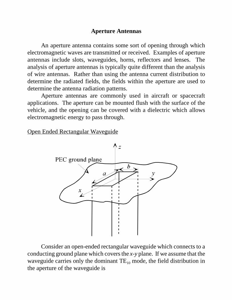
Aperture Antennas

An aperture antenna contains some sort of opening through whichelectromagnetic waves are transmitted or received. Examples of apertureantennas include slots, waveguides, horns, reflectors and lenses. Theanalysis of aperture antennas is typically quite different than the analysisof wire antennas. Rather than using the antenna current distribution todetermine the radiated fields, the fields within the aperture are used todetermine the antenna radiation patterns.

Aperture antennas are commonly used in aircraft or spacecraftapplications. The aperture can be mounted flush with the surface of thevehicle, and the opening can be covered with a dielectric which allowselectromagnetic energy to pass through.

Open Ended Rectangular Waveguide

Consider an open-ended rectangular waveguide which connects to aconducting ground plane which covers the x-y plane. If we assume that thewaveguide carries only the dominant TE10 mode, the field distribution inthe aperture of the waveguide is

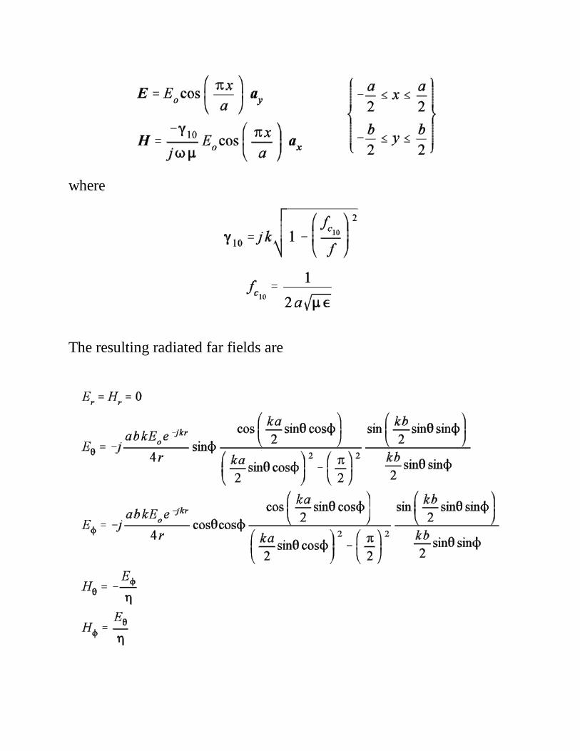
where

The resulting radiated far fields are

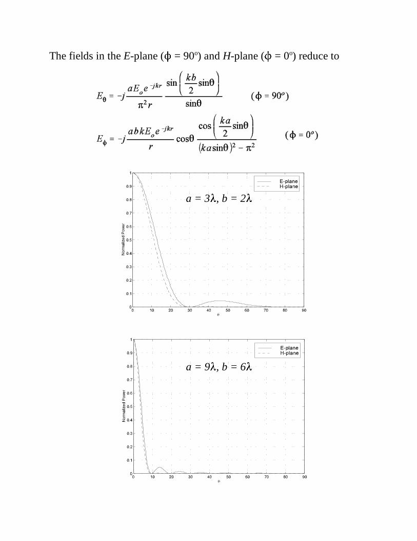
The fields in the E-plane ( = 90o) and H-plane ( = 0o) reduce to

a = 3, b = 2

a = 9, b = 6

Horn Antennas

The horn antenna represents a transition or matching section from theguided mode inside the waveguide to the unguided (free-space) modeoutside the waveguide. The horn antenna, as a matching section, reducesreflections and leads to a lower standing wave ratio. There are three basictypes of horn antennas: (a.) the E-plane sectoral horn (flared in thedirection of the E-plane only), (b.) the H-plane sectoral horn (flared in thedirection of the H-plane only), and (c.) the pyramidal horn antenna (flaredin both the E-plane and H-plane). The flare of the horns considered hereis assumed to be linear although some horn antennas are formed by otherflare types such as an exponential flare.

The horn antenna is mounted on a waveguide that is almost alwaysexcited in single-mode operation. That is, the waveguide is operated at afrequency above the cutoff frequency of the TE10 mode but below thecutoff frequency of the next highest mode.

E-Plane Sectoral Horn

E-plane Sectoral Horn E-plane Far Field ( = /2)

E-plane Sectoral Horn H-plane Far Field ( = /2)

The directivity of the E-plane sectoral horn (DE) is given by

A plot of the E-plane and H-plane patterns for the E-plane hornshows that the H-plane pattern is much broader than the E-plane pattern.Thus, the E-plane sectoral horn tends to focus the beam of the antenna inthe E-plane (see Figures 13.3 and 13.4).

Design curves for the E-plane sectoral horn are given in Figure 13.8.

Example (E-plane sectoral horn design, Problem 13.6)

An E-plane horn is fed by a WR 90 (X-band) rectangular waveguide(a = 2.286 cm, b = 1.016 cm). Design the horn so that its maximumdirectivity at 11 GHz is 30 (14.77 dB).

H-Plane Sectoral Horn

H-plane Sectoral Horn E-plane Far Field ( = /2)

H-plane Sectoral Horn H-plane Far Field ( = /2)

The directivity of the H-plane sectoral horn (DH) is given by

A plot of the E-plane and H-plane patterns for the H-plane hornshows that the E-plane pattern is much broader than the H-plane pattern.Thus, the H-plane sectoral horn tends to focus the beam of the antenna inthe H-plane (see Figures 13.11 and 13.12). Design curves for the H-planesectoral horn are given in Figure 13.16.

Pyramidal Horn

Based on the pattern characteristics of the E-plane and H-planesectoral horns, the pyramidal horn should focus the beam patterns in boththe E-plane and the H-plane. In fact, the E-plane and H-plane patterns ofthe pyramidal horn are identical to the E-plane pattern of the E-planesectoral horn and the H-plane pattern of the H-plane sectoral horn,respectively (See Figure 13.19).

The directivity of the pyramidal horn (DP) can be written in terms ofthe directivities of the E-plane and H-plane sectoral horns:

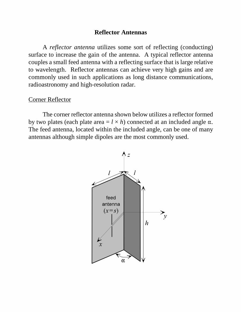
Reflector Antennas

A reflector antenna utilizes some sort of reflecting (conducting)surface to increase the gain of the antenna. A typical reflector antennacouples a small feed antenna with a reflecting surface that is large relativeto wavelength. Reflector antennas can achieve very high gains and arecommonly used in such applications as long distance communications,radioastronomy and high-resolution radar.

Corner Reflector

The corner reflector antenna shown below utilizes a reflector formedby two plates (each plate area = l × h) connected at an included angle .The feed antenna, located within the included angle, can be one of manyantennas although simple dipoles are the most commonly used.

The most commonly used included angle for corner reflectors is90o. The electrical size of the aperture (Da) for the corner reflector antennais typically between one and two wavelengths. Given a linear dipole as thefeed element of a 90o corner reflector antenna, the far field of this antennacan be approximated using image theory. If the two plates of the reflectorare electrically large, they can be approximated by infinite plates. Thisallows the use of image theory in the determination of the antenna far field.

For analysis purposes, the current on the feed element is assumed tobe z-directed. The image element #2 represents the image of the feedelement (#1) to plate #1. Together, elements #1 and #2 satisfy the electricfield boundary condition on plate #1. Similarly, image element #3represents the image of the feed element to plate #2. In order for imageelement #2 to satisfy the electric field boundary condition on plate #2, anadditional image element (#4) is required. Note that the inclusion of imageelement #4 also allows image element #3 to satisfy the electric fieldboundary condition on plate #1. The system of four elements (four-element array) yields the overall field within the included angle of thereflector antenna (45o 45o). The four- element array can be treatedas 2 two-element arrays (a two-element array along the x-axis and the two-element array along the y-axis).

Given a two-element array aligned along thez-axis with equal amplitude, equal phase elementswhich are separated by a distance 2s, the resultingarray factor was found to be

If we rotate this 2-element array so that it lies alongthe x-axis, we must transform the array factoraccording to

which yields

Similarly, rotating the two-element array so that it lies along the y-axis, andnoting that the current is opposite to that of the array along the x-axis, wefind

The overall array factor for the 90o corner reflector becomes

In the azimuth plane ( = /2), the 90o corner reflector array factor is

The corner reflector array factor can be shown to be quite sensitive to theplacement of the feed element, as would be expected. The following plotsshow the azimuth plane array factor for various feed spacings.

s = 0.1 s = 0.7

s = 0.8 s = 1.0

A variety of reflecting surface shapes are utilized in reflectorantennas. Some reflector antennas employ a parabolic cylinder as thereflecting surface while a more common reflecting surface shape is theparaboloid (parabolic dish antenna). The so-called Cassegrain antennauses dual reflecting surfaces (the main reflector is a paraboloid, the sub-reflector is a hyperboloid).