Research Division Federal Reserve Bank of St. Louis Working Paper Series

Education Policies and Structural Transformation

Pedro Cavalcanti Ferreira Alexander Monge-Naranjo

and Luciene Torres de Mello Pereira

Working Paper 2014-039A http://research.stlouisfed.org/wp/2014/2014-039.pdf

October 2014

FEDERAL RESERVE BANK OF ST. LOUIS

Research Division P.O. Box 442

St. Louis, MO 63166

______________________________________________________________________________________

The views expressed are those of the individual authors and do not necessarily reflect official positions of the Federal Reserve Bank of St. Louis, the Federal Reserve System, or the Board of Governors.

Federal Reserve Bank of St. Louis Working Papers are preliminary materials circulated to stimulate discussion and critical comment. References in publications to Federal Reserve Bank of St. Louis Working Papers (other than an acknowledgment that the writer has had access to unpublished material) should be cleared with the author or authors.

Education Policies and Structural Transformation

Pedro Cavalcanti Ferreira� Alexander Monge-Naranjo. y

Luciene Torres de Mello Pereira z

October 29, 2014

Abstract

This article studies the impact of education and fertility in structural transformation andgrowth. In the model there are three sectors, agriculture, which uses only low-skill labor,manufacturing, that uses high-skill labor only and services, that uses both. Parents chooseoptimally the number of children and their skill. Educational policy has two dimensions,it may or may not allow child labor and it subsidizes education expenditures. The modelis calibrated to South Korea and Brazil, and is able to reproduce some key stylized factsobserved between 1960 and 2005 in these economies, such as the low (high) productivityof services in Brazil (South Korea) which is shown to be a function of human capital andvery important in explaining its stagnation (growth) after 1980. We also analyze how di¤er-ent government policies towards education and child labor implemented in these countriesa¤ected individuals�decisions toward education and the growth trajectory of each economy.JEL classi�cation codes: J13, J24, O40, O41, O47, O57Keywords: economic growth, structural transformation, education, fertility

�EPGE/FGV, Rio de Janeiro.yFederal Reserve Bank of St. Louis and Washington University in St. Louis.zEPGE/FGV, Rio de Janeiro.

1 Introduction

In the last �fty years, some economies experienced episodes of rapid and sustained economic

growth, while others had episodes of high growth followed by stagnation and even recession.

South Korea and Brazil are examples of these two distinct paths.

The Brazilian economy experienced high productivity and output growth until the early 80�s,

in a clear catch-up process relative to the leading economies. The country presented one of the

highest growth rates in the world and ceased to be predominantly rural to become urban, with

production concentrated in manufacturing and service sector. However, in the early 80�s, Brazil

began to reverse this catch-up process and productivity began to fall1.

South Korea, despite having levels of per capita output and relative productivity below Brazil

until the mid-80�s, experienced an uninterrupted growth process throughout the entire period

(1960 to 2005). This was due to the high growth of the Korean average productivity, which can

be summarized with the following fact: until the mid-60�s, the productivity of a Korean worker

was only 60% of the Brazilian, however in 2005 a worker in South Korea was on average more

than twice as productive as the Brazilian. The exemplary Korean growth was also possible due

to government policies which promoted education that enabled the formation of skilled labor for

manufacturing and service sector. In contrast, a large part of Brazilian stagnation in the 80�s and

90�s can be explained by economic, educational and social policies.

The di¤erences between the Brazilian and Korean productivities since mid-80�s may be con-

sequence of an accelerated or a meager growth of some productive sector. An hallmark of the

economic development of countries, and documented in the literature, is the process of structural

transformation. In this process, there is a displacement of resources between di¤erent productive

sectors (agriculture, manufacturing and services) over time. In general, the economies initially

undergo a reduction in the share of agricultural sector and an increase in the importance of man-

ufacturing and service sector in the workforce and in the production. This process usually causes

an increase in aggregate productivity of economies, since labor productivity in agriculture is usu-

ally smaller than in the other two sectors. In a second stage of structural transformation, the

importance of manufacturing falls and the share of services sector (in terms of labor and value

added) dominates the economy.

The literature2 indicates the low growth in the service sector as the main cause for the stagna-

tion of the Brazilian economy and the decline in relative productivity after the 80�s. Therefore, the

1See Figure 1.2See [Duarte and Restuccia, 2010] and [Silva and Ferreira, 2011].

2

question of what would be the cause of the poor performance of this sector naturally arises. The

data indicate a massive reallocation of labor from agriculture toward the service sector, while the

percentage of workers in manufacturing remained stable during the period 1960 to 2005 in Brazil.

As in general, the labor employed in agriculture is of low quali�cation, an argument sustained in

this paper is that the �ow of unskilled labor to services is a possible cause for the poor performance

of the sector. Regarding South Korea, we can say that almost all workers who left agriculture

went toward the service sector, as pointed out by [Kim and Topel, 1995]. Thus, both economies

went through a quite similar structural transformation process. However, sector growth was quite

di¤erent: South Korea had in the period faster growth in manufacturing - at an annualized rate

of 5.5% - as opposed to less than 3% in Brazil, and the service sector grew by 2% a year in Korea

but virtually zero in Brazil3.

To understand the dissimilar development experience of these two countries, we propose a

structural transformation model that incorporates human capital decision, in which the trade-

o¤ between the quantity of children and the quality of education faced by parents is a¤ected

by government policies. In the model, there will be two types of workers, skilled and unskilled

(or high- and low-skill), and three sectors, agriculture, manufacturing and services. Agriculture

employs only unskilled labor; manufacturing, only skilled labor and the service sector employs both

types. Therefore, the structural transformation is stylized, in the sense that there will be in a �rst

moment reallocation of unskilled labor from agriculture to the services, and then reallocation of

skilled labor from manufacturing to the service sector.

The type of quali�cation of each adult will be determined by the investment of his parents

during his childhood. Parents chooses optimally the number of o¤springs and their skill. Educa-

tional policy has two dimensions, it may or may not allow child labor and it subsidizes education

expenditures.

The model is calibrated to the Brazilian and South Korean economies and is able to reproduce

the main stylized facts observed between 1960 and 2005. In addition, we performed some coun-

terfactual exercises, which measures the importance of educational policies to the accumulation of

human capital and how it a¤ects the process of structural transformation.

This article relates to several literatures. Regarding the structural transformation literature,

this process was �rst documented as a stylized fact of economic growth by [Kuznets, 1973]. Our

paper is closer to the recent literature that aims to understand episodes of accelerated growth, stag-

3It is worth noting that while Brazil remained closed to trade and adopted a policy of import substitutionindustrialization during almost the entire period, Korea opened the economy to international trade and implementedpolicies to stimulate exports and industrialization. However, this point is not emphasized in this study.

3

nation and decline stressing productivity di¤erences across sectors and the reallocations of labor

between them4. The article of [Timmer and de Vries, 2009] argues that the episodes of growth are

explained by increases in productivity across sectors and concludes that improvements in produc-

tivity in the service sector are more important than the growth of productivity in manufacturing5.

In [Duarte and Restuccia, 2010], the authors investigate the role of sectoral labor productivity in

structural transformation and in the trajectory of aggregate productivity of 29 countries. They

are able to �nd large di¤erences in agriculture and service productivity but a minor di¤erence in

manufacturing sector. They also noted that the catch-up process in the productivity of manufac-

turing is responsible for half of the productivity gains, while the low productivity of the service

sector explains all the experiences of stagnation and economic decline. [Silva and Ferreira, 2011]

investigates the same issue of [Duarte and Restuccia, 2010] in six Latin American countries in the

period of 1950-2003. They came to the conclusion that the service sector was generally responsible

for the reversal of the catch-up process, which occurred since the 80�s.

[Betts et al., 2013] and [Kim and Topel, 1995] study structural transformation in South Ko-

rea. [Betts et al., 2013] examines, quantitatively and qualitatively, the role of international trade

and (distorting) trade policies in the reallocation of labor and production, using a model of

three sectors and two countries (Korea and OCDE), with labor as the only factor of produc-

tion. [Kim and Topel, 1995] analyzes the evolution of the labor market in South Korea during

an episode of extraordinary economic growth (1970-1990), with industrialization and structural

transformation process as their background. They found that the fraction of workers employed

in agriculture fell by 30 percentage points in less than 20 years and there is no evidence that

agricultural workers migrated to manufacturing. Indeed, employment growth in manufacturing

occurred only by recruiting new entrants (with higher human capital) in the labor market, which

tend to stay in this sector throughout their career.

This article is also related to the fertility and education literature, which began with

the work of [Becker, 1960] and nowadays is quite extensive6. [Becker et al., 1990] studies the

interaction of fertility and education decisions with economic development. It assumes endogenous

fertility and a rising rate of return on human capital. There are two steady states: a Malthusian

regime, where wages are constant and fertility is high, and a growth regime with rising wages and

low fertility. The model, however, is not able to generate the transition between stagnation and

4 [Herrendorf et al., 2013] presents an extensive literature review and recent advances.5 [Herrendorf and Valentinyi, 2012] also aims to answer which sectors are responsible for low productivity in

developing countries.6A major review of literature with relevant criticisms is presented in [Jones et al., 2010].

4

growth. [Doepke, 2004] is able to �ll this gap. Furthermore, [Doepke, 2004] was probably the �rst

to consider the role of fertility decisions in the discussion of growth and inequality7. In the paper,

the transition from Malthusian stagnation to the modern growth regime can be generated from a

relatively simple model, based on the trade-o¤ between quantity and quality of children faced by

individuals. This article also introduces particular government policies - which we follow closely

in our paper - in order to produce di¤erent transition paths for each country. It also introduces

to the model child labor, taken as an opportunity cost of the infant. The model is calibrated to

Brazil and South Korea

[Mbiekop, 2013] develops a model of structural transformation that incorporates the choice

of human capital. The model has just two productive sectors (agriculture and manufacturing)

and the supply of skilled labor increases the productivity of manufacturing, which is intensive

in this type of labor, while agriculture uses only unskilled labor. Results depend mainly on the

educational composition of the workforce and so the paper focuses on human capital accumulation

as an engine of economic development of African countries8.

In certain aspects, this paper presents several contributions to these literatures. It incorporates

fertility and education decisions, and consequently the formation of human capital to the structural

transformation models. Thus, labor ceases to be purely homogeneous. Therefore, the characteri-

zation of the structural transformation process becomes richer. We use this framework to propose

an explanation for the decline in service productivity pointed by [Duarte and Restuccia, 2010]

and [Silva and Ferreira, 2011], since 1980 in Brazil (also in other Latin American economies).

Furthermore, it is the �rst paper in the fertility and education literature to consider three con-

sumer goods. Moreover, the analysis of the model takes place via a general equilibrium model,

while [Erosa et al., 2010] and [Mbiekop, 2013] are based in partial equilibrium analysis. Similar to

[Badel et al., 2013] we study human capital formation in a three sectors structural transformation

model. However, we incorporate fertility decisions and abstract from migration and urbanization

decisions, which is key to their analysis

This paper proceed as follows. In the next section, the data is described in details. In section

3, stylized facts of Brazilian and Korean economies and some motivations are presented. In section

4, the model and the equilibrium are described, taking into account the inclusion of public policies.

In section 5, we present the analytical results of the model. In section 6, the model is calibrated

7See also [Moav, 2005] and [de la Croix and Doepke, 2003].8 [Erosa et al., 2010] presents a model of heterogeneous agents in order to quantify the importance of di¤erences

in human capital versus TFP to explain variations in per capita income across countries. The model has two sectors- manufacturing and services -, and fertility and education decisions, but does not study structural transformation.

5

with the intention to reproduce the allocations of di¤erent types of labor between productive

sectors and the distribution of skills in population of the two countries. In section 7, the numerical

results are presented, i.e., the results generated by the model are compared with the data and we

perform some counterfactuals. Finally, section 8 concludes.

2 Data

The sample covers Brazil, South Korea and United States9 and the years between 1955 and 2005.

However, the period chosen for study is between 1960 and 2005. This occurs because the

�ve early years of the sample period were chosen as the basis period for productivity in order

to generate variability in productivity across the sectors at the next periods10. The series

of value added and employment by sectors were taken from [McMillan and Rodrik, 2011].

The [McMillan and Rodrik, 2011] data is composed by the Groningen Growth and Develop-

ment Centre (GGDC) database, which provides statistics of employment and real value

added for 27 countries (among them, Brazil and South Korea) disaggregated into 10 sectors

([Timmer and de Vries, 2007] and [Timmer and de Vries, 2009]) with the inclusion of data from

African countries, China and Turkey. The reason to use [McMillan and Rodrik, 2011] database is

that the authors converted the value added to international dollars of 2000 and took into account

the purchasing power parity (PPP).

The value added and employment data cover ten productive sectors, but in this paper they

were grouped into three major sectors (agriculture, manufacturing and services), following the

structural transformation literature. The ten production sectors are de�ned by the ISIC Rev.311

de�nitions and were grouped as follows: agriculture includes agriculture, forestry and �shing (01-

05), manufacturing is composed by mining and extraction (10-14), manufacturing (15-37), utilities

(40-41) and construction (45), and the service sector consists of wholesale and retail trade, hotels

and restaurants (50-55), transport, storage and communication (60-64), �nance, insurance and

real estate (65-74), and community, social, personal and government services (75-99).

The hours worked data in the ten productive sectors was obtained from di¤erent sources for

each country. For South Korea, this series was obtained easily from the EU KLEMS database12.

However, this data is only available for the years 1970-2005. No data are available on hours

9This only for comparison of the productivity trajectory of Brazil and South Korea.10It will be be explained with more details in the section Calibration.11International Standard Industrial Classi�cation of All Economic Activities, Rev.3.12See [O�Mahony and Timmer, 2009].

6

worked in Brazil13. Thus we had to generate it from PNAD (Pesquisa Nacional por Amostra de

Domicílio14), a household survey that covers all regions of Brazil and interviews more than 300.000

people every year since 197615.

Following the structural transformation literature, the productivity series was constructed as

the ratio between the value added and the total number of hours worked by sector for each economy

and for the period 1955-2005.

From the [Barro and Lee, 2010] database we obtained the share of the population percentage

that has primary, secondary or tertiary education. These data are used as variables of human

capital accumulation for each country and compared with the model results.

3 Stylized Facts

After World War II, Brazil was still a poor country and predominantly agricultural. However,

between 1960 and 1980, the country underwent a profound transformation. During this period,

the Brazilian economy grew very fast. Until the late 70s, there was a catch-up process relative to

the United States (U.S.). As can be seen in Figure 1, the Brazilian income per capita was only 20%

of U.S. income in 1960, but after 20 years it was already 35% of the U.S.. Note that the relative

output per worker followed the same trend of income per capita, with only a small di¤erential.

However, since 1980 we can observe a drastic growth slowdown. The relative income per capita

and output per worker began to fall and the convergence process was reversed. Only after the

2000s these variables showed signs of recovery, remaining practically constant until 200516.

South Korea is a successful example of economic growth. In 1960, the Korean economy was

approximately half of Brazil (in terms of income per capita and output per worker), and in 2005,

it was already half of the U.S. economy and twice as big as Brazil. From Figure 1, we can see that

South Korea experienced a continuous process of catch-up17. During the 1960-2005 years, South

Korea had one of the highest growth rates in the world. In a short period, the country became a

developed and industrialized economy.

13There is a time series that covers only the metropolitan regions for the period 1992-2005 provided byLABORSTA.14National Household Survey conducted every year in Brazil (see Appendix A and

www.ibge.gov.br/home/estatistica/populacao/trabalhoerendimento/pnad2005/ for more details).15Since the period of interest is 1955-2005, we had to repeat for the previous years the data of 1970 and of 1976

for South Korea and Brazil, respectively.16Note that relative productivity in Brazil by the end of the period was at the same level that in 1960, about

20%.17Due to the Asian crisis of 1997, there was a decline in economic growth, which was reversed rapidly and in

1999, the country has returned to grow.

7

These two growth trajectories that initially were very similar but from 1980 became quite

di¤erent pose the following question: what went wrong with Brazil? When the attention falls

on government policies, a very important di¤erence is education. While Brazil barely invested

in human capital formation, South Korea adopted policies such as education subsidy and child

labor restriction. When focusing in sectorial contribution to growth, there are indications that the

service sector was they main culprit for the low growth of Brazil.

3.1 Structural Transformation

From Figure 2, we observe the evolution of the relative share of workers employed in agriculture,

manufacturing and services in Brazil between 1960 and 200518. In 1960, about 58% of Brazilian

workers were still in agriculture, 17% in manufacturing and 25% in services. Over time, manu-

facturing participation in the labor force has had little change, growing only 2 percentage points

between 1960 and 2005. However, there was an important reallocation of workers from agriculture

toward services. In 2005, about 62% of the workforce was in the service sector and only 19% was

in agriculture. Thus, we can say that the structural transformation occurred signi�cantly between

agricultural and service sectors.

Still in Figure 2, we observe the evolution of labor allocation across the productive sectors

in South Korea. Similar to Brazil, there was a massive transfer of workers from agriculture to

services: the share of labor of the agricultural sector fell from 69% in 1960 to 8% in 2005, while

the service share rose from 21% to 63%. Regarding the share of workers in manufacturing, it grew

until 1991, felt in the next seven years and then has stabilized since 1998. Although it appears

that there was also a migration of workers from agriculture to industry, [Kim and Topel, 1995]

shows, from a cohort analysis, that this kind of reallocation actually did not happen. In fact there

was a change in the workforce composition in the sense that greater participation of workers in

manufacturing was due to the entry of new individuals (with a higher education level) in the labor

market who have decided to go to this sector.

Figure 3 shows the evolution of productivity19 in the three sectors between 1960 and 2005 in

both countries. In Brazil, there is a clear upward trend in the productivity of the agricultural and

manufacturing sectors, and a rise followed by a fall in service productivity. Furthermore, through-

out the period agricultural productivity is well below those of the other two sectors. Between 1960

and 1980, the three productive sectors showed signi�cant growth, with agricultural and service

18In this initial analysis, we assumed homogeneous labor.19Here de�ned as output per worker.

8

productivity growing at similar rates (2.6% per year) while manufacturing grew at a higher rate

(4% per year). In this period there is a signi�cant reallocation of workers from agriculture to

services. Given that the service was more productive than agriculture, this reallocation led to

an acceleration of the Brazilian aggregate productivity, which resulted in convergence. However,

since 1980, service productivity fell signi�cantly (a negative growth rate of 2.5% per year between

1980 and 2005) and manufacturing stagnated. Considering the increasing share of workers em-

ployed in the service sector (over 60% of Brazilian labor force in 2005) and the continuous fall

of productivity in this sector, it is easy to understand the reversal of the catch-up process in the

Brazilian economy. Thus, it seems that the ine¢ ciency of the service sector is behind the fall in

productivity growth and in per capita income.

In South Korea, one can observe a continuous productivity growth in all the three sectors dur-

ing the entire period (1960-2005). Manufacturing experienced very high growth, 5.5% annualized.

Agriculture also had a considerable growth in productivity (5.4% per year). The productivity

growth of service sector was much lower, with a rate of about 2% per year. Although the perfor-

mance of services has been less than the other two sectors, the growth of productivity contributed

positively to reducing its economic gap relative to United States. In summary, while the service

sector can be seen as the main responsible for Brazilian stagnation, Korean economic success can

be explained by the good performance of all three productive sectors, in particular services, which

employs the highest percentage of workers.

3.2 Education

In the post World War II, Brazil adopted an economic development project of import substitution,

characterized by strong stimulus to investment in physical capital in manufacturing, nationaliza-

tion of public utility services and steep barriers to international trade20. Education was not a

priority so that the country experienced a low level of investment in the sector, particularly in

public primary education. The low investment in education along with a very high rate of pop-

ulation growth (and high fertility rate, although declining, as can be seen in Figure 5) led to the

relatively unskilled workforce observed in later years.

Although free and compulsory basic education is provided by law since 1930 in Brazil, in

practice public schools are of poor quality and primary education does not reach many rural areas

until now. The neglect of the government with the universalization of education over time can be

20For more details, see [Veloso et al., 2013].

9

perceived from the educational expenditures. Table 2 (taken from [Maduro Junior, 2007]) shows

the low investment in education (as a proportion of GDP) by the government until the 1980 and

the disproportion between investment per student in the primary and tertiary levels (in 1960, a

student in tertiary education costs 117 times more than one in primary education). Moreover, for

many years the Brazilian government was very tolerant with child labor: despite having established

since its 1934 Constitution the minimum age of 14 for employment, this was never enforced in the

country. In 1985, 18.7% of the children between ages 10 and 14 were in the labor market.21

South Korea, after the Korean War (1950-1953), instituted a plan of compulsory and free

basic education, which led to a high enrollment rate already in 1960. Furthermore, the education

control was gradually withdrawn from local administrations (provinces) and concentrated in the

Ministry of Education, which became responsible for the administration of schools, the allocation

of resources, the development of school curriculum, among other tasks. Restrictions on child labor

were taken very seriously since the Korean independence. Although the country has signed only

in 1991 the International Labor Organization (ILO) convention that rules out child labor under

the age of 14, since 1960 the participation rates of Korean children in workforce were very low:

1.1% of children between 0 and 15 years in 1960 and only 0.3% in 1985, according to the ILO.

Di¤erent public policies of education and child labor implemented in Brazil and South Korea

have produced, as expected, di¤erent results. Figure 6 shows the evolution of average years

of schooling of the Brazilian and Korean population. In 1960, the di¤erence between the two

countries was only 1.4 years, but in 2005 this di¤erential rose to 4.5 years. Tables 4 and 5 show

the evolution of the percentage of Brazilian and Korean population with certain educational levels.

In 1960 the percentage with no schooling was almost the same in the two economies, but over

time the situation improved in Korea way more than in Brazil, so that in 2005, this �gure was

three times higher in Brazil than in South Korea. When we look to the proportion of people who

have the primary, secondary and tertiary education, South Korea always had higher percentages

in high educational levels (secondary and tertiary) and population growth in these two levels was

also higher than in Brazil. Therefore, analyzing only the years of study of each economy, the

Korean evolution was more favorable. We can also analyze enrollment ratios. Table 3 shows the

evolution of enrollment rates in primary and secondary education levels. Although Brazil and

Korea present primary rate very similar over the years, Korea has a large and growing advantage

in the rates of secondary education, which further illustrates the better educational level of the

21And child labor is even more persistent among male children, with 25.3% of them in the Brazilian workforcein 1987 and 24.3% in 1990, according to [Doepke, 2004].

10

Korean population. Although the two countries have very similar primary enrollment rates, this

measure overestimates educational level in Brazil, because it was not taken into consideration the

quality of education22.

4 Model

We consider a standard dynastic OLG economy extended with endogenous fertility and multiple

production sectors. Indviduals live for two periods. The investments of young individuals (chil-

dren) in human capital determine their skill levels when old. Old individuals (adults) decide how

to allocate their time between child rearing and working. They must also choose in which of the

three sectors of the economy to work: agriculture, manufactures and services. Adults can also

choose how many children to have and how much to invest in their education. In our analysis we

introduce education policies in a model that combines the main elements of Barro-Becker [XXX]

and subsequent models in the quantity/quality trade-o¤ literature and the non-homotheticity in

consumption used in recent structural transformation models.23

In any given period, the utility V of an adult depends on a vector c = (cA; cM ; cS) of consump-

tion levels of agricutural goods, manufactures and services. It is also a function of the number of

children and their utility when old. In our baseline model, we restrict our analysis to two types of

children: low-skill24 (denoted by the subindex L) and high-skill25 (denoted by the subindex H).

Consider an adult with consumption c, nL low-skill children and nH high-skill children who

are, respectively, expected to attain utilities V0H , V

0L when old. We assume that such an adult

attains an utility level

V (c; nH ; nL) = U (c) + �(nH + nL)�"[nHV

0

H + nLV0

L],

where

U (c) =

�v(cA)(cM)

b(cS + �cS)(1�b)�1��

1� � .

Here v(cA) = 1 if cA � �cA and v(cA) = 0 otherwise. For tractability, we assumed that food is not

valued beyond a subsistance threshold �cA. As for the other parameters: b governs the share of

manufacturing vis-à-vis services; �cS � 0 is a positive parameter that indicates that services are a22For comparisons between the quality of education in the countries, see test results from PISA (Programme for

International Student Assessment), conducted every three years since 2000.23See [Doepke, 2004] and [Duarte and Restuccia, 2007] for leading examples of papers in these two lines of work.24In this paper, unskilled and low-skill have the same meaning.25In this paper, skilled and high-skill have the same meaning.

11

superior good; 0 < � < 1 is the inverse of the intertemporal elasticity of substitution; we assume

� < 1 to keep the values the utility being positive. Finally, " governs the curvature of the parental

altruism as a function of the quantity of children.26 These parameters will play an important role

for the transition dynamics of the economy.

Adults are endowed with one unit of time, which can be allocated between working in the

marketplace or raising children (at home). Raising each child requires a fraction 0 < � < 1 of

time, regardless of the skills level of the parent. But parents not only decide on the number of

children (quantity) but also on their education (quality). On one hand, parents can opt to keep

(some of) the children unschooled, and they will be low-skill adults. On the other hand, parents

can opt to invest in school for their children. Schooling a child requires teachers and only high-skill

adults can supply teaching services. For a child to become a high-skill worker when old, he must

also receive 0 < �H < 1 units of time from a teacher. Thus, the (opportunity) cost of just having

a child varies proportionally with the skills of the the parent, but the absolute cost of providing

him with schooling is the same for all parents regardless of their skills.

We consider two simple government policies. One is the extend to which child labor is allowed.

In our stylized environment, children that are not attending school might remain idle (e.g. watching

TV) or parents can put them to work. A working child can provide 0 < �L < � units of low skill

labor. Also, we assume that children who work do not attend school and become low-skill adult.

As in Doepke (2004), we assume that restrictions imposed by governments imply that parents of

unschooled children can extract at most 0 � �gL � �L units of low-skill labor. Those restrictionsare relevant since they can reduce the cost of having unschooled children.27

The other government policy we consider is a subsidy on education. Speci�cally, we assume

that the government subsidizes a fraction 0 < � < 1 of the schooling costs. These subsidies

are �nanced with a proportional tax on earnings � . We assume that the rate � is exogenously

given and that the tax rate evolves over time, according to the state of the economy, so that the

government budget is balanced each period, as we explain further below. Both policies f�gL, �gshape up the fertility and human capital investment decisions of parents, and the production of

the three sectors in the economy.

There are three production sectors in the economy: agriculture (A), manufacturing (M), and

services (S). We use agriculture goods as the numeraire, and pM and pS are the prices of manufac-

turing and services relative to that numeraire. Aside from the non-homotheticities in preferences,

26See [Becker et al., 1990].27However, since �U < �, the overall net cost of having a child is positive and fertility is strictly below the

biological upper bound 1=�.

12

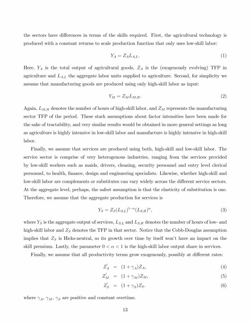
the sectors have di¤erences in terms of the skills required. First, the agricultural technology is

produced with a constant returns to scale production function that only uses low-skill labor:

YA = ZALA;L. (1)

Here, YA is the total output of agricultural goods, ZA is the (exogenously evolving) TFP in

agriculture and LA;L the aggregate labor units supplied to agriculture. Second, for simplicity we

assume that manufacturing goods are produced using only high-skill labor as input:

YM = ZMLM;H . (2)

Again, LM;H denotes the number of hours of high-skill labor, and ZM represents the manufacturing

sector TFP of the period. These stark assumptions about factor intensities have been made for

the sake of tractability, and very similar results would be obtained in more general settings as long

as agriculture is highly intensive in low-skill labor and manufacture is highly intensive in high-skill

labor.

Finally, we assume that services are produced using both, high-skill and low-skill labor. The

service sector is comprise of very heterogenous industries, ranging from the services provided

by low-skill workers such as maids, drivers, cleaning, security personnel and entry level clerical

personnel, to health, �nance, design and enginnering specialists. Likewise, whether high-skill and

low-skill labor are complements or substitutes can vary widely across the di¤erent service sectors.

At the aggregate level, perhaps, the safest assumption is that the elasticity of substitution is one.

Therefore, we assume that the aggregate production for services is

YS = ZS(LS;L)1��(LS;H)

�; (3)

where YS is the aggregate output of services, LS;L and LS;H denotes the number of hours of low- and

high-skill labor and ZS denotes the TFP in that sector. Notice that the Cobb-Douglas assumption

implies that ZS is Hicks-neutral, so its growth over time by itself won�t have an impact on the

skill premium. Lastly, the parameter 0 < � < 1 is the high-skill labor output share in services.

Finally, we assume that all productivity terms grow exogenously, possibly at di¤erent rates:

Z0

A = (1 + A)ZA, (4)

Z0

M = (1 + M)ZM , (5)

Z0

S = (1 + S)ZS. (6)

where A, M , S are positive and constant overtime.

13

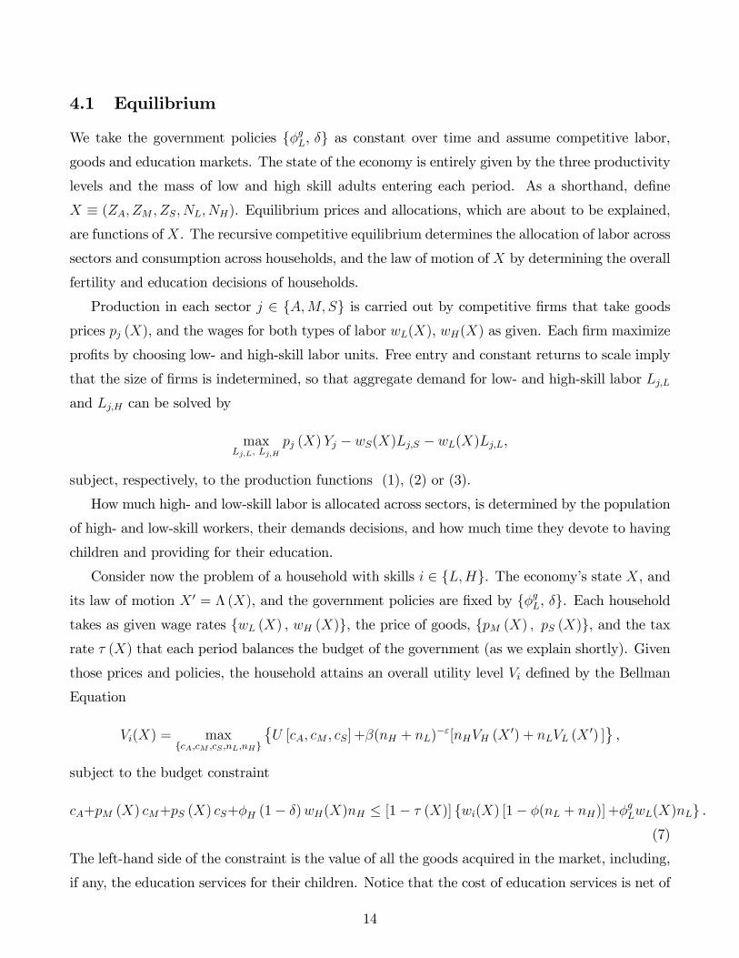
4.1 Equilibrium

We take the government policies f�gL, �g as constant over time and assume competitive labor,goods and education markets. The state of the economy is entirely given by the three productivity

levels and the mass of low and high skill adults entering each period. As a shorthand, de�ne

X � (ZA; ZM ; ZS; NL; NH). Equilibrium prices and allocations, which are about to be explained,

are functions of X. The recursive competitive equilibrium determines the allocation of labor across

sectors and consumption across households, and the law of motion of X by determining the overall

fertility and education decisions of households.

Production in each sector j 2 fA;M; Sg is carried out by competitive �rms that take goodsprices pj (X), and the wages for both types of labor wL(X), wH(X) as given. Each �rm maximize

pro�ts by choosing low- and high-skill labor units. Free entry and constant returns to scale imply

that the size of �rms is indetermined, so that aggregate demand for low- and high-skill labor Lj;L

and Lj;H can be solved by

maxLj;L, Lj;H

pj (X)Yj � wS(X)Lj;S � wL(X)Lj;L,

subject, respectively, to the production functions (1), (2) or (3).

How much high- and low-skill labor is allocated across sectors, is determined by the population

of high- and low-skill workers, their demands decisions, and how much time they devote to having

children and providing for their education.

Consider now the problem of a household with skills i 2 fL;Hg. The economy�s state X, andits law of motion X 0 = � (X), and the government policies are �xed by f�gL, �g. Each householdtakes as given wage rates fwL (X) , wH (X)g, the price of goods, fpM (X) ; pS (X)g, and the taxrate � (X) that each period balances the budget of the government (as we explain shortly). Given

those prices and policies, the household attains an overall utility level Vi de�ned by the Bellman

Equation

Vi(X) = maxfcA;cM ;cS ;nL;nHg

�U [cA; cM ; cS] +�(nH + nL)

�"[nHVH (X0) + nLVL (X

0) ],

subject to the budget constraint

cA+pM (X) cM+pS (X) cS+�H (1� �)wH(X)nH � [1� � (X)] fwi(X) [1� �(nL + nH)] +�gLwL(X)nLg .

(7)

The left-hand side of the constraint is the value of all the goods acquired in the market, including,

if any, the education services for their children. Notice that the cost of education services is net of

14

government subsidies. The right hand side includes all the earnings of the household, including,

if any, the earnings of working unschooled children.28

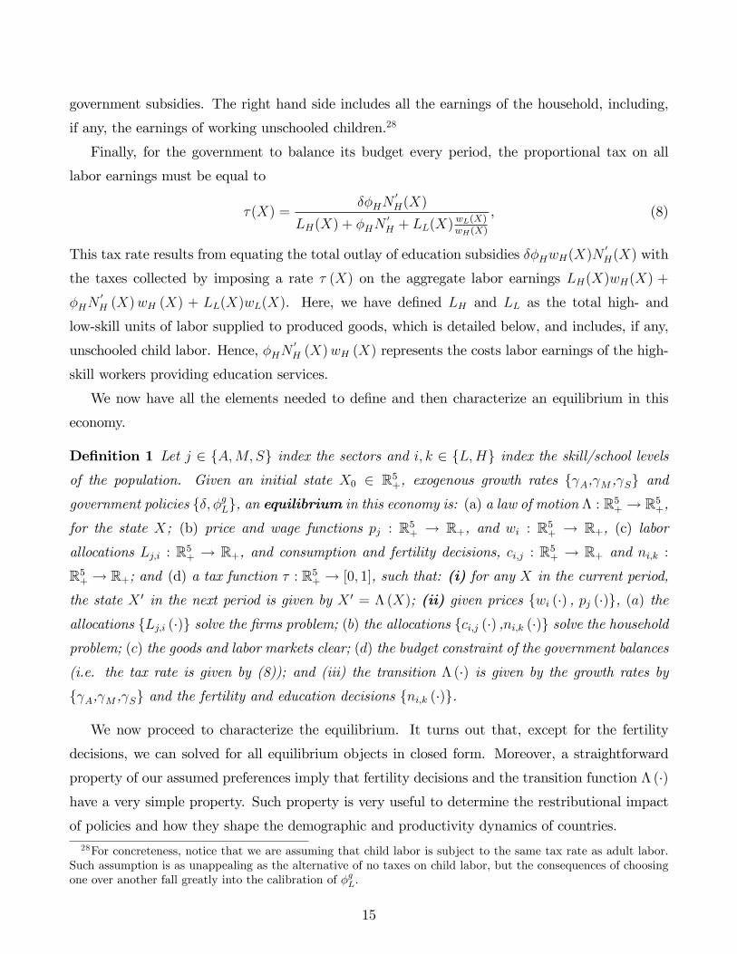
Finally, for the government to balance its budget every period, the proportional tax on all

labor earnings must be equal to

�(X) =��HN

0H(X)

LH(X) + �HN0H + LL(X)

wL(X)wH(X)

, (8)

This tax rate results from equating the total outlay of education subsidies ��HwH(X)N0H(X) with

the taxes collected by imposing a rate � (X) on the aggregate labor earnings LH(X)wH(X) +

�HN0H (X)wH (X) + LL(X)wL(X). Here, we have de�ned LH and LL as the total high- and

low-skill units of labor supplied to produced goods, which is detailed below, and includes, if any,

unschooled child labor. Hence, �HN0H (X)wH (X) represents the costs labor earnings of the high-

skill workers providing education services.

We now have all the elements needed to de�ne and then characterize an equilibrium in this

economy.

De�nition 1 Let j 2 fA;M; Sg index the sectors and i; k 2 fL;Hg index the skill/school levelsof the population. Given an initial state X0 2 R5+, exogenous growth rates f A, M , Sg andgovernment policies f�; �gLg, an equilibrium in this economy is: (a) a law of motion � : R5+ ! R5+,for the state X; (b) price and wage functions pj : R5+ ! R+, and wi : R5+ ! R+, (c) laborallocations Lj;i : R5+ ! R+, and consumption and fertility decisions, ci;j : R5+ ! R+ and ni;k :R5+ ! R+; and (d) a tax function � : R5+ ! [0; 1], such that: (i) for any X in the current period,

the state X 0 in the next period is given by X 0 = � (X); (ii) given prices fwi (�) , pj (�)g, (a) theallocations fLj;i (�)g solve the �rms problem; (b) the allocations fci;j (�) ,ni;k (�)g solve the householdproblem; (c) the goods and labor markets clear; (d) the budget constraint of the government balances

(i.e. the tax rate is given by (8)); and (iii) the transition � (�) is given by the growth rates byf A, M , Sg and the fertility and education decisions fni;k (�)g.

We now proceed to characterize the equilibrium. It turns out that, except for the fertility

decisions, we can solved for all equilibrium objects in closed form. Moreover, a straightforward

property of our assumed preferences imply that fertility decisions and the transition function � (�)have a very simple property. Such property is very useful to determine the restributional impact

of policies and how they shape the demographic and productivity dynamics of countries.28For concreteness, notice that we are assuming that child labor is subject to the same tax rate as adult labor.

Such assumption is as unappealing as the alternative of no taxes on child labor, but the consequences of choosingone over another fall greatly into the calibration of �gL.

15

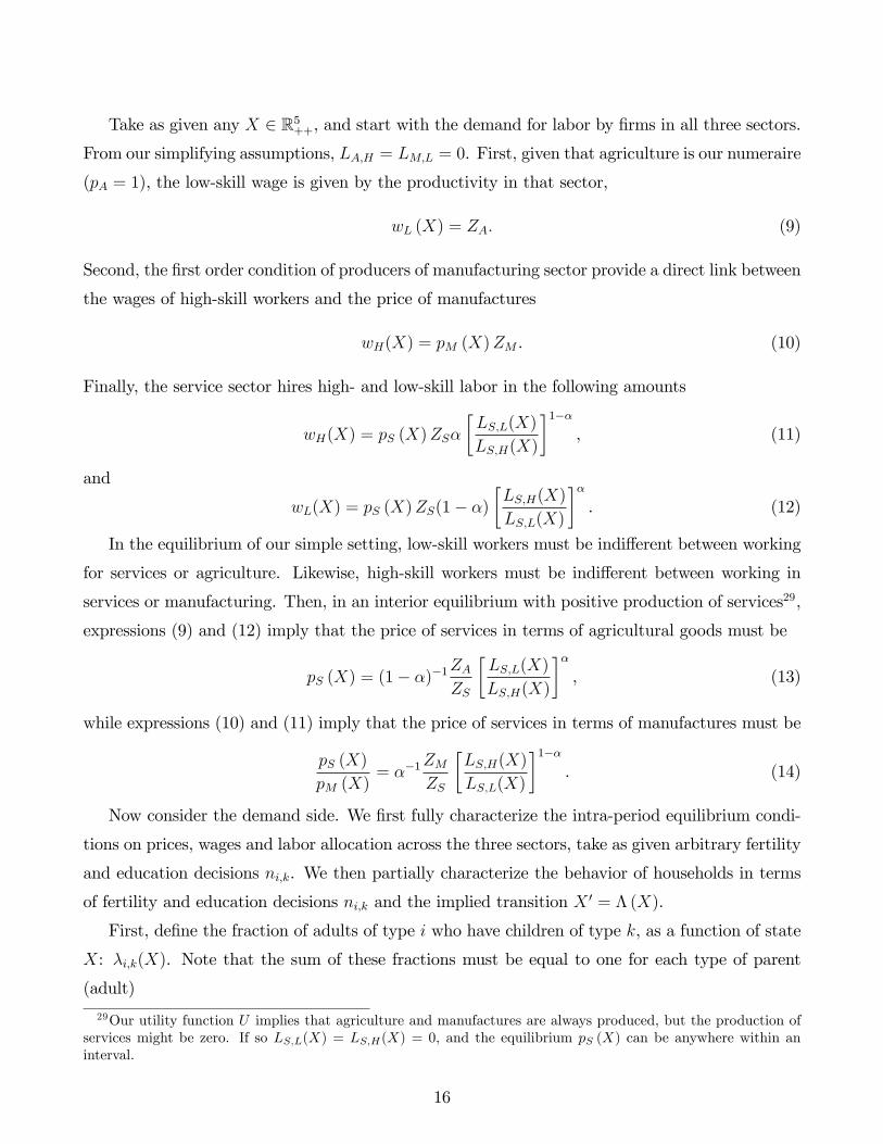
Take as given any X 2 R5++, and start with the demand for labor by �rms in all three sectors.From our simplifying assumptions, LA;H = LM;L = 0. First, given that agriculture is our numeraire

(pA = 1), the low-skill wage is given by the productivity in that sector,

wL (X) = ZA: (9)

Second, the �rst order condition of producers of manufacturing sector provide a direct link between

the wages of high-skill workers and the price of manufactures

wH(X) = pM (X)ZM . (10)

Finally, the service sector hires high- and low-skill labor in the following amounts

wH(X) = pS (X)ZS�

�LS,L(X)

LS,H(X)

�1��, (11)

and

wL(X) = pS (X)ZS(1� �)�LS,H(X)

LS,L(X)

��. (12)

In the equilibrium of our simple setting, low-skill workers must be indi¤erent between working

for services or agriculture. Likewise, high-skill workers must be indi¤erent between working in

services or manufacturing. Then, in an interior equilibrium with positive production of services29,

expressions (9) and (12) imply that the price of services in terms of agricultural goods must be

pS (X) = (1� �)�1ZAZS

�LS,L(X)

LS,H(X)

��, (13)

while expressions (10) and (11) imply that the price of services in terms of manufactures must be

pS (X)

pM (X)= ��1

ZMZS

�LS,H(X)

LS,L(X)

�1��. (14)

Now consider the demand side. We �rst fully characterize the intra-period equilibrium condi-

tions on prices, wages and labor allocation across the three sectors, take as given arbitrary fertility

and education decisions ni;k. We then partially characterize the behavior of households in terms

of fertility and education decisions ni;k and the implied transition X 0 = � (X).

First, de�ne the fraction of adults of type i who have children of type k, as a function of state

X: �i;k(X). Note that the sum of these fractions must be equal to one for each type of parent

(adult)

29Our utility function U implies that agriculture and manufactures are always produced, but the production ofservices might be zero. If so LS,L(X) = LS,H(X) = 0, and the equilibrium pS (X) can be anywhere within aninterval.

16

�H;H(X) + �H;L(X) = �L;H(X) + �L;L(X) = 1:

Now, consider the fertility and education decisions ni;k as given. This means, that each low

-skill household supplies [1� � (nL;L + nL;H)]+�gLnL;L units of low-skill labor. In turn, each high-skill household provides [1� � (nH;L + nH;H)] units of high-skill labor and �gLnH;L units of low-skilllabor. Therefore, the aggregate supply of high- and low-skill labor, LH and LL, available for the

production of consumption goods are, respectively, given by

LH = NH [1� � (�H;LnH;L + �H;HnH;H)]� �H (NH�H;HnH;H +NL�L;HnL;H) , (15)

LL = NL [1� � (�L;LnL;L + �L;HnL;H)] + �gL (NH�H;LnH;L +NL�L;LnL;L) ,

where the high-skill labor required to educate the next crop of high-skill workers is subtracted in

the �rst expression, while the low-skill labor supplied by children is added in the second expression.

In terms of LH and LL, the �rst order conditions of producers from the three sectors lead to simple

equilibrium of prices and quantities. First, since pA = 1, the wage of low-skill labor is entirely

determined by the productivity of the agricultural sector,

wL (X) = ZA.

Second, from the assumed form for the demand for agricultural goods, the low-skill labor used in

that sector is

LA;L =�cAZA(NL +NH).

The remaining low-skill workers are employed in the service sector

LS;L = LL ��cAZA(NL +NH).

In a similar vein, if LM;H � LH units of high-skill labor are allocated to manufactures, then theremaining LH �LM;H workers are in services. Then, from equation (14), the indi¤erence betweenhigh-skill workers about working for the manufactures or services sectors imply

pS (X)

pM (X)= ��1

ZMZS

�LH � LM;HLS;L

�1��. (16)

The other determinant of relative prices and of how labor is allocated across sectors is the demand.

Given our assumption of Stone-Geary preferences it is easy to show that each household of skill

level i will equate the marginal rate of substitution between manufactures cM;i and services cS;i,

i.e.(1� b) cM;ib [cS;i + �cS]

=pS (X)

pM (X).

17

Since Stone-Geary preferences are Gorman aggregable, the equilibrium relative prices pS (X) =pM (X)

must satisfypS (X)

pM (X)=

(1� b)ZMLM;Hb�ZS (LL;S)

1�� (LH � LM;H)� + �cS(NL +NH)� . (17)

Then, equating (16) and (17) and simplifying, leads to the condition�1 +

� (1� b)b

�LH;M = LH +

�cS(NL +NH)

ZS

�LL �

�cAZA(NL +NH)

�1�� [LH � LH;M ]1�� .Clearly, given any level LH , as long as LL >

�cAZA(NL +NH), there is a uniquely de�ned allocation

0 < LM;H < LH of high-skill labor between manufactures and services. As a function of LM;H ,

the LHS is strictly increasing and is zero when LM;H = 0; the RHS is strictly decreasing in LH;M ,

and when LH;M = 0 its value is positive. Moreover, when all labor is allocated to manufacturing,

LM;H = LH , then the LHS is strictly greater than the RHS.

Here: discussion of comparative statics. ERE.

We now examine the determination of ni;k, the fertility and human capital decisions of children.

Let ei �P

j pjcj;i denote the expenditure in goods of a household with skills i. The budget

constraint can be re-written as

ei = �wi (X)� Ei;

where �wi (X) � [1� � (X)]wi (X) are the net-of taxes potential (or full) labor market earnings ofthe household and Ei � [1� � (X)] f[wi (X)�(nL + nH)]� �gLwL(X)nLg + �H (1� �)wH(X)nH ,is the amount of resources spent in children.

Following Doepke (2004), the fertility/schooling decisions can be solved as a problem of choos-

ing the total amount spend in children and the compostion of the family between high- and

low-skill. To this end, �rst notice that the period, indirect utility function can be written as

�U = U ( �wi (X)� Ei;X) =1

1� �

(�b ( �wi (X)� E � �cA + pS (X) �cS)

pM (X)

�b �(1� b) ( �wi (X)� E � �cA + pS (X) �cS)

pS (X)

�1�b)1��.

Second, we write what are the full prices of high- and low-skill children. The former cost the

parent

pi;H (X) = � �wi (X) + (1� �)�HwH (X) ,

i.e. the time cost plus the cost of education, both net of taxes and subsidies. Similarly, each

low-skill child costs the parent

pi;L (X) = � �wi (X)� �gL �wL (X) ,

18

i.e. the time cost plus minus the earnings from child labor, both net of taxes. Obviously, E =

nLpi;L (X) + nHpi;H (X).

Adults take the alternative future utilities VL (X 0) and VH (X 0) of their children as given. Since

we are assuming that � < 1, we can restrict our analysis to the cases in which 0 < VL (X0) �

VH (X0), where the second inequality holds because high-skill individuals can always opt for the

occupations and fertility choices of the low-skilled. We can rewrite the problem as one choosing

total expenditure E and the fraction f of E that is spent on raising high-skill children. Thus,

the number of high-skill children is nH = f � E=pi;H , and the number of low-skill children isnL = (1� f) � E=pi;L. Plugging those expressions, the fertility/human capital problem of an

adult can be written as:

max0�E� �wi;0�f�1

�U ( �wi (X)� E; X)+�E1�"

�f

pi;H+(1� f)pi;L

��fVH (X

0)

pi;H+(1� f)VL (X 0)

pi;L

��. (18)

Under these preferences, low skill and high skill children are perfect substitutes, i.e. the

indi¤erence curves are straight lines for the parents. The relative prices pi;H , pi;L and the utilities

VL (X0), VH (X 0) determine the family composition in a stark form.

Proposition 2 For all fE; fg, that attains the maximum in (18), the solution is f = 0 or f = 1,i.e., the problem of adult has only corner solutions.

Proof. See Appendix B.

Adults choose to have only one type of child so that there is never both types of children in

the same family. Given this result, it is possible to determine the optimal number of children

by assuming that parents have a single type k, where k 2 fH;Lg. While it is not possible toexplicitly solve the equation above for nk30, the separability of preferences imply that children are

superior goods:

Proposition 3 Conditional on the type k 2 fH;Lg of children, the optimal number of childrennk is increasing in the futute utility Vk (X 0) and the net of taxes full income �wi (X).

Proof. See Appendix B

Therefore, children are a normal good. Another important property of the adult�s problem is

described in the following proposition:

30These problems are straightforward to computed, as described in detail in Appendix D.

19

Proposition 4 An adult is indi¤erent between both types of children if, and only if, the costs and

utilities of children satisfy the following condition:

VH (X0)

(pi;H)1�" =

VL (X0)

(pi;L)1�" (19)

If an adult is indi¤erent, the total expenditure on children does not depend on the type of child

chosen.

Proof. See Appendix B.

The above propositions generate important implications for the mobility between generations.

Since in equilibrium wH > wL, nurturing high-skill children is relatively cheaper for high-skill

parents than for low-skill parentspH;HpH;L

<pL;HpL;L

. (20)

High-skill parents have a "comparative advantage" in the "production" of high-skill children,

while the low-skill parents have a "comparative advantage" in the "production" of low-skill chil-

dren. Moreover, as the relative price of children di¤ers between the types of parents, it is not

possible that both types of adults remain indi¤erent between the two types of kids at the same

time. And given the comparative advantage, in equilibrium there will be always high-skill parents

who have high-skill children, as well as there will be always low-skill parents who have low-skill

children.

We have to de�ne what kind of parent will be indi¤erent between the two types of kids. Since

the interest of this model is to generate upward intergenerational mobility, this equilibrium path

occurs only when low-skill adults are indi¤erent between the two types of children. In this case, all

high-skill parents have high-skill children, while the low-skill parents have both types of children.

We have then the following corollary.

Corollary 5 For any X such that wH(X) > wL(x), it must be true that:

� A positive fraction of high-skill adults have high-skill children and a positive fraction of low-skill adults have low-skill children:

�H;H (X) , �L;L (X) > 0:

20

� Only one type of adult can be indi¤erent between the two types of children:

�H;L (X) > 0 =) �L;H (X) = 0;

�L;H (X) > 0 =) �H;L (X) = 0.

Add: Proposition. Impact on policy. Given fptk; wti,� tg the e¤ect of changes in policies, equi-librium with upward mobility: (a) child labor, increase welfare of low skill, increase fertility; (b)

education subsidies, increasse welfare and fertility of high skill.

Discussion of taxes and GE.

5 Calibration

We need to determine the value of the preference parameters �, �, ", b, �cA, and �cS; the parameters

representing the cost of raising a child (�), educational cost (�H), child labor productivity (�L),

government subsidy to education (�); and coe¢ cient of the production function of services (�).

Moreover, we have to �nd the time series of productivity of each sector Aj, where j 2 fA;M; Sg.To �nd the productivity series, �rst we have to de�ne the amounts of high- and low-skill labor

employed in the service sector. Given our very stylized production functions, we have to use a not so

rigorous de�nition of high-skill labor: individuals with the secondary level education (incomplete)

are considered highly skilled. Had we opted, for instance, to associate highly skilled with college

education the number of high-skill labor in 1960 would be very small and way smaller than the

observed labor in manufacturing in both countries. The evolution of the percentage of high-skill

individuals in the two countries is given by Table 6, that uses data from [Barro and Lee, 2010]31.

Returning to the issue of the amount of low and high-skill labor employed in the service

sector, �rst we need to make some points clear. Although the de�nition described below seems

somewhat arbitrary, it was the only one found so that comparable data between Brazil

and Korea (from [McMillan and Rodrik, 2011]) could be used. We classify the subsectors which

comprise the service sector as skilled or unskilled. When we analyze the wage di¤erential of the

service subsectors in relation to manufacturing (assumed to employ only high-skill labor), we can

see from [Medeiros, 2012] that the workers employed in transport, storage and communication

31Note that in the model a period comprises 25 years. However, there are only data available, for both countries,from 1960 to 2005.

21

(60-64) or in �nancial activities, insurance, real estate and administrative services (65-74) receive

a higher wage than those in manufacturing. And since wage re�ects the labor productivity, we

argue that the workers in these two sectors are all highly skilled. But when we analyze the

wholesale and retail trade, hotels and restaurants (50-55) subsector, we realize a negative (and

statistically signi�cant) di¤erential. So we conclude that the low-skill labor is predominant in this

subsector. It remains to consider personal services (social community, personal and government

services (75-99)) subsector. Note that it is quite heterogeneous, but we only have data available for

the countries in this level of aggregation (from GGDC database). Although education and health

are activities that pay a higher wage (relative to manufacturing), they are relatively smaller (in

terms of labor) than the other two (other community, social and personal services, and private

households with employed persons). And since these two sectors have a negative wage di¤erential,

we considered the whole personal services as a sector that employs only low-skill labor. Although

all the above analysis has been done with Brazilian data (PNAD), we assumed earlier that both

countries have the same production functions, so we argue that these labor de�nitions are also

valid for Korea.

From the de�nition above of high- and low-skill labor, service productivity is obtained according

to (3). Before this, however, we must �rst determine the value of �. This parameter represents

the share of high-skill workers in the total income of the service sector. We used data from

PNAD, the Brazilian household survey, and two di¤erent methodologies to calculate �: In the �rst

methodology, we considered workers with less than nine years of education as lowly skilled. We

then multiply the number of individuals in this group by their average income32 to obtain total

income of low-skill workers, and divided it by the income of the entire services sector.

In the second methodology, we classi�ed sectors as low-skill or high-skill using a de�nition close

to that discussed in the previous paragraph. For each low-skill sector we multiply the number of

workers (that were considered to be all lowly skilled) by the average labor income of the sector.

We then added the income of all low-skill sectors and divided by the total income of the service

sector. We found that the participation of low-skill labor in the total income of services to vary

between 0.35 to 0.41, depending on the methodology or whether we included public sector or not.

We set � = 0:40: We found similar values when using surveys form di¤erent years.

In the literature, productivity dispersion across sectors is crucial for the process of structural

transformation to contribute to productivity growth. Thus, for each country and each period the

32Actually the PNAD does not have information on the exact years of schooling of an individual, but only onintervals of schooling - e.g., "one or less year of education" or "between six and nine years of education". Wemultiply the total number of individuals by the average income of each interval.

22

average productivity for the period 1955-1959 is normalized to one, i.e., AA;55�59 = AM;55�59 =

AS;55�59 = 1. Denoting j as the productivity growth rate of the sector j for in a single period, the

productivity of the �rst (1960-1982) and second (1983-2005) periods are respectively Aj;60�82 =

(1 + j)Aj;55�59 and Aj;83�05 = (1 + j)2Aj;55�59, where Aj;60�82 is the average productivity of

period 1960-1982 and Aj;83�05 is the average productivity of period 1983-2005.

Most of the parameters are the same for both countries. The intertemporal preference parame-

ters (�, �, and ") were calibrated following [Doepke, 2004], while the intratemporal preference pa-

rameters followed [Herrendorf et al., 2011] and [Duarte and Restuccia, 2007]. The parameters of

manufacturing (b) and services (1� b) weights followed the calibration of [Herrendorf et al., 2011].Since a developed economy generally spends a smaller fraction of their income in the agri-

cultural goods, the parameters �cA and �cS depend on the level of development of each country.

Therefore, these two parameters were calibrated for each country (Brazil and Korea) and each pe-

riod (�rst and second). The parameter �cA was computed so that the model reproduced the share

of low-skill labor employed in agriculture. And �cS was chosen to minimize the distance between

the product and the consumption of service.

The calibration of education costs parameters follows [Doepke, 2004]. Furthermore, the fraction

of the education cost paid by the government was chosen to be 0.5, as in [Doepke, 2004]. And we

assumed that in Korea there was a partially restriction on child labor initially, but in the second

period this type of labor was completely abolished. For Brazil, it was assumed no education

subsidy by the government and no restrictions on child labor over the years.

6 Numerical Results

6.1 Benchmark Economies

The model reproduces closely the allocations of the di¤erent types of labor across the three pro-

ductive sectors, at the initial (1960-1982) and �nal (1983-2005) periods. Table 7 presents the

results for the initial period. The proportion of low-skill labor employed in agriculture generated

by the model is slightly below, but very close to the data in the two countries. The proportion of

high-skill labor in manufacturing is slightly above but close to the actual values. Table 8 presents

the results for the �nal period. The allocation of low-skill labor in agriculture produced by the

model are only 1 p.p. higher than the actual value in the two economies. With respect to the

allocation of high-skill labor in manufacturing, the model is able to reproduce the data in Brazil

and misses by only 5 p.p. in Korea. Therefore, the process of structural transformation of the two

23

economies is nicely explained by the model.

Results regarding the proportion of high-skill individuals in the economies are not so good

as the labor allocations. This problem occurs for both countries. From Tables 7 and 8, we can

observe for Brazil that there is an overestimation of this variable by 21 p.p. initially, but it drops

to just 9 p.p. at the �nal period. For South Korea, there is also a considerable overestimation

(di¤erence of 20 p.p.), but it falls to only 4 p.p. at the �nal period and the model reproduces very

well the data. This high deviation, especially at the initial period, may be due to the fact that

all workers employed in manufacturing were considered highly skilled. And since manufacturing

was initially more developed in the two countries and employed proportionally more workers, this

could have led tho the overestimation of high-skill individuals by the model. But the model seems

to reproduce more closely the �nal period of the two economies, especially the Korean.

Given the distribution of high-skill individuals and the allocations of the di¤erent types of

labor in productive sectors, we can also obtain with the benchmark model the growth rate of the

per capita output. The Brazilian benchmark economy produces a growth rate of 36% between

the two periods and the Korean per capita output grows by 232%. According to the Penn-World

Table Brazil basically stagnate in the period (a negative growth of 8%) and Korean grew by 207%.

Hence, although overestimating slightly growth in both cases, the model reproduces the order of

magnitude and the relative �gures very well. We will use these �gures to compare the e¤ect of

di¤erent types of counterfactuals exercises in the growth of the economies at the next subsection.

6.2 Counterfactuals

The �rst class of these counterfactuals is to check what would happen to the economy of each

country if other public policies had been adopted. In Table 9 we analyze the case in which Brazil

subsidizes education and restricts child labor, following Korean second period policies. Initially

this policy change does not a¤ect the economy, since the values of the variables of interest are

very similar to those in Tables 7 and 8. However at the second period, the proportion of high-

skill individuals increases substantially, going from 36% in benchmark model to 60%. This result

indicates that the policies implemented by Korea would produce a considerable accumulation of

human capital if they had been implemented in Brazil.

This policy also does not produce major changes at the �rst period in the allocation of labor

between sectors. However at the next period it is able to prevent a massive reallocation of low-skill

workers from agriculture to the service sector. Therefore, the low-skill labor now represents less

than half of all labor employed in the service sector, i.e., high-skill labor becomes the majority

24

in the sector. Furthermore, if these public policies were implemented in Brazil, the growth rate

of per capita output would be 57% between the two periods, i.e., 21 p.p. above the growth of

the Brazilian benchmark economy (36%). Hence, in an annual base Brazil would grow almost 1%

faster, without changing the path of sectorial productivities, had he adopted better educational

policies.

In the case of Korea (Table 10), we run an experiment in which policies are such that there is

no education subsidy and no child labor restriction. Initially, there is just a small decrease in the

proportion of high-skill individuals compared to the benchmark model, and the sector allocations

remains virtually unchanged. However, in the second period there is a considerable decrease in the

proportion of high-skill individuals in the economy, dropping from 74% in the benchmark model

to 42%. In addition, between the �rst and second period the number of skilled workers grows very

little.

Due to this low human capital accumulation, Korea would end up following a trajectory very

similar to that observed in Brazil, with a massive migration of low-skill labor from the agricultural

sector to services. In this case the period growth rate of the Korean economy falls to only 112%,

about half of the growth in the benchmark economy (232%). The smaller supply of high-skill

labor negatively a¤ects the production of manufactured goods and services, that are growing fast

in the period and becoming dominant.

In a second group of counterfactual exercises countries switch sectorial productivities with

each other. When Brazil is given South Korean productivities, from Table 11 we see that the

distribution of high-skill individuals in the economy increases in both periods when compared

with the benchmark results shown in Tables 7 and 8 (increase of 11 p.p. and 8 p.p. respectively).

The distribution of skilled and unskilled labor (in percentage terms) is quite similar to those of the

Korean benchmark model. Furthermore, the period growth rate of the Brazilian economy would

be 125%, i.e., about three times larger than the growth rate of the benchmark economy.

With South Korea experiencing the Brazilian sectorial productivities, results in Table 12 shows

that although the percentage of highly quali�ed individuals has fallen relative to the benchmark

model (67% and 74%, respectively), this decrease is small, especially when compared with the

results of the other counterfactual exercises for Korea. The reallocation of high- and low-skilled

labor across sectors in the second period is such that two thirds of the low-skill labor is allocated in

services, and 60% of high-skill labor goes to manufacturing, a result very similar to the benchmark

simulation of Brazil. Moreover, with Brazilian productivities, South Korea output grows only 49%

between the two periods, way less than in the benchmark economy (232%).

25

When comparing the growth rates of the two classes of counterfactuals with those of the

benchmark economies, one can see that productivity in manufacturing explains a large portion of

the output growth, while the low productivity levels in services (which in this case is the result

of a massive allocation of unskilled labor to this sector) play a key role in explaining episodes of

growth slowdown or stagnation. The di¤erent roles played by the secondary and tertiary sectors

had already been discussed in the literature (e.g., [Duarte and Restuccia, 2010]), but not the role

of human capital accumulation. In the counterfactual exercise in which Brazil implements South

Korean educational policies, its period growth rate increases by 20 p.p. This is the result of a

greater human capital accumulation, which reverted the poor performance of the service sector.

Similarly when we assume that South Korea adopts Brazilian educational policies, the proportion

of second period high-skill workers fall from 74% in the benchmark simulation to just 42%, leading

to a fall in the growth rate of output of approximately 50% (from 232% to 112%).

Note however, that results in the second group of counterfactuals are such that the growth rate

in Brazil, 125%, is much greater than in the �rst counterfactual. This so because South Korean

manufacturing productivity is very high in the period (1983-2005) and leads to a large gain in the

Brazilian overall productivity and growth. Note, however, that the impact in this case is large not

only because of the direct e¤ect of the very high TFPs of South Korea on Brazilian output but

because of an indirect e¤ect on human capital formation: the proportion of high-skill labor jumps

from 31% in the �rst period to 42% and in the second period it goes from 35% to 44%. Human

capital accumulation is still very important.

The third class of counterfactuals is to verify the impact of each public policy separately33.

In the case of Brazil, from Table 13, it is possible to see that child labor restriction has a very

signi�cant impact on the economy. The percentage of high-skill individuals grows with this policy

compared with the benchmark economy, from 31% to 48% initially, and in the second period, the

growth is even higher, from 35% to 61%. There is also a greater concentration of low-skill labor

in agriculture. Manufacturing maintains the same labor concentration than in the benchmark

economy in both periods. The impact of education subsidy in the economy is smaller, the increase

in the proportion of high-skill individuals is just 7 p.p. in the �rst period and 10 p.p. in the second.

Moreover, in the two periods there is a higher concentration of low-skill labor in agriculture, and

the percentage of high-skill labor remains stable and very close to that of the benchmark economy.

In the case of South Korea, the absence of child labor restrictions has an impact of only 1 p.p.

33Note, however, that it is di¢ cult to consider the two policies separately because child labor restriction mustbe incentive compatible and there is a clear link between the cost of education and child labor. So the resultspresented below must be seen with a caveat in mind.

26

in the percentage of high-skill individuals in the economy (see Table 14). This fact results from

the hypothesis adopted in the �rst period of the benchmark economy that child labor is partially

banned in South Korea. In the second period, when this kind of work is totally prohibited, the

impact of relaxing this restriction is signi�cant, amounting to a drop of 20 percentage points.

The allocations of the two types of labor in the �rst period remains similar to the benchmark

economy, but in the second period, there is a larger concentration of low-skill individuals in the

service sector. Similarly to Brazil, the impact of education subsidy is smaller when considering its

e¤ects on the formation of high-skill individuals. A no-subsidy policy produces a decrease in the

formation of human capital of, respectively, 8 p.p. and 5 p.p. in the �rst and second periods.

7 Conclusion

In the second half of the last century, Brazil and South Korea had episodes of accelerated economic

growth. However, since the 80�s, the Brazilian economy has stagnated and the ine¢ cient service

sector is pointed by the structural transformation literature as the responsible. The hypothesis

sustained is that the negative growth of labor productivity in the service sector is due to migration

of low-skill workers from agriculture to service sector.

We have proposed a model that combines the elements of the structural transformation litera-

ture to the microeconomic approach of education and fertility choices. Furthermore, we considered

in the model public policies of education subsidy and child labor restrictions. The model provided

a good distribution of quali�cation levels in the population of the two countries, as well as the

labor allocations between sectors. With counterfactual exercises, we concluded that policies of

education subsidy and child labor restriction are essential for the accumulation of human capital

in the economies, with the latter having a higher impact. The greater participation of high-skill

individuals in the economy is able to avoid a greater allocation of low-skill workers in the service

sector. Furthermore, comparing the growth paths (growth rates) produced by the counterfactual

exercises with those produced by the benchmark economies we had the same conclusions pointed by

[Duarte and Restuccia, 2010] and [Silva and Ferreira, 2011]. Therefore, using a micro-foundations

approach, this article was able to compare and explain the processes of transformation structural,

which were initially very similar between Brazil and South Korea, but from a certain point became

di¤erent.

27

References

[Badel et al., 2013] Badel, A., Ferreira, P. C., and Monge-Naranjo, A. (2013). Human capital and

the urban and structural transformation of countries. Manuscript.

[Barro and Lee, 2010] Barro, R. J. and Lee, J.-W. (2010). A new data set of educational attain-

ment in the world, 1950â¼AS2010. NBER Working Papers 15902, National Bureau of Economic

Research, Inc.

[Becker, 1960] Becker, G. S. (1960). An economic analysis of fertility. In Demographic and Eco-

nomic Change in Developed Countries, NBER Chapters, pages 209�240. National Bureau of

Economic Research, Inc.

[Becker et al., 1990] Becker, G. S., Murphy, K. M., and Tamura, R. (1990). Human capital,

fertility, and economic growth. Journal of Political Economy, 98(5):S12�37.

[Betts et al., 2013] Betts, C., Giri, R., and Verma, R. (2013). Trade, reform, and structural

transformation in south korea. MPRA Paper 49540, University Library of Munich, Germany.

[de la Croix and Doepke, 2003] de la Croix, D. and Doepke, M. (2003). Inequality and growth:

Why di¤erential fertility matters. American Economic Review, 93(4):1091�1113.

[Doepke, 2004] Doepke, M. (2004). Accounting for fertility decline during the transition to growth.

Journal of Economic Growth, 9(3):347�383.

[Duarte and Restuccia, 2007] Duarte, M. and Restuccia, D. (2007). The structural transformation

and aggregate productivity in portugal. Portuguese Economic Journal, 6(1):23�46.

[Duarte and Restuccia, 2010] Duarte, M. and Restuccia, D. (2010). The role of the structural

transformation in aggregate productivity. The Quarterly Journal of Economics, 125(1):129�

173.

[Erosa et al., 2010] Erosa, A., Koreshkova, T., and Restuccia, D. (2010). How important is human

capital? a quantitative theory assessment of world income inequality. Review of Economic

Studies, 77(4):1421�1449.

[Herrendorf et al., 2011] Herrendorf, B., Rogerson, R., and Valentinyi, A. (2011). Two perspec-

tives on preferences and structural transformation. IEHAS Discussion Papers 1134, Institute of

Economics, Hungarian Academy of Sciences.

28

[Herrendorf et al., 2013] Herrendorf, B., Rogerson, R., and Valentinyi, A. (2013). Growth and

structural transformation. NBER Working Papers 18996, National Bureau of Economic Re-

search, Inc.

[Herrendorf and Valentinyi, 2012] Herrendorf, B. and Valentinyi, A. (2012). Which sectors make

poor countries so unproductive? Journal of the European Economic Association, 10(2):323�341.

[Jones et al., 2010] Jones, L. E., Schoonbroodt, A., and Tertilt, M. (2010). Fertility theories:

Can they explain the negative fertility-income relationship? In Demography and the Economy,

NBER Chapters, pages 43�100. National Bureau of Economic Research, Inc.

[Kim and Topel, 1995] Kim, D.-I. and Topel, R. H. (1995). Labor markets and economic growth:

Lessons from korea s industrialization, 1970-1990. In Di¤erences and Changes in Wage Struc-

tures, NBER Chapters, pages 227�264. National Bureau of Economic Research, Inc.

[Kuznets, 1973] Kuznets, S. (1973). Modern economic growth: Findings and re�ections. American

Economic Review, 63(3):247�58.

[Maduro Junior, 2007] Maduro Junior, P. R. (2007). Taxas de matriculas e gastos em educacao

no brasil. Economics working papers, Graduate School of Economics (EPGE), Getulio Vargas

Foundation (FGV).

[Mbiekop, 2013] Mbiekop, F. (2013). A simple model of structural transformation for small,

agriculture-based open economies. Working paper, CIRPEE and Department of Economics,

Universite du Quebec a Montreal.

[McMillan and Rodrik, 2011] McMillan, M. S. and Rodrik, D. (2011). Globalization, structural

change and productivity growth. NBER Working Papers 17143, National Bureau of Economic

Research, Inc.

[Medeiros, 2012] Medeiros, B. L. (2012). Diferencial de salarios e produtividade no setor de ser-

vicos brasileiro. Economics working papers, Graduate School of Economics (EPGE), Getulio

Vargas Foundation (FGV).

[Moav, 2005] Moav, O. (2005). Cheap children and the persistence of poverty. Economic Journal,

115(500):88�110.

29

[O�Mahony and Timmer, 2009] O�Mahony, M. and Timmer, M. P. (2009). Output, input and

productivity measures at the industry level: The eu klems database. Economic Journal,

119(538):F374�F403.

[Silva and Grossi, 1997] Silva, J. F. G. d. and Grossi, M. d. (1997). A mudanca do conceito de

trabalho nas novas pnads. Economia e Sociedade, IE, Unicamp, -(5):247�261.

[Silva and Ferreira, 2011] Silva, L. F. d. and Ferreira, P. C. (2011). Structural transformation and

productivity in latin america. Economics Working Papers 724, Graduate School of Economics

(EPGE), Getulio Vargas Foundation (FGV).

[Timmer and de Vries, 2007] Timmer, M. P. and de Vries, G. J. (2007). A cross-country database

for sectoral employment and productivity in asia and latin america, 1950-2005. Technical report.

[Timmer and de Vries, 2009] Timmer, M. P. and de Vries, G. J. (2009). Structural change and

growth accelerations in asia and latin america: a new sectoral data set. Cliometrica, Journal of

Historical Economics and Econometric History, 3(2):165�190.

[Veloso et al., 2013] Veloso, F., Ferreira, P. C., and Giambiagi, Fabio e Pessoa, S. (2013). Desen-

volvimento Economico: Uma Perspectiva Brasileira. Elsevier.

30

A Appendix: Data

The average number of hours worked per year in each of the nine productive sectors (ISIC Rev. 3)

over the period of interest (1955-2005) for Brazil was built from the PNAD database. The PNAD

is a national household survey conducted every year in Brazil since 1976.

The geographical scope, the concept of work (occupied person) and the classi�cation of eco-

nomic activities have changed over the years. Regarding the geographical scope, since 1976 PNAD

have already covered the Northeast, Southeast and South, the Federal District and metropolitan

areas of the North and of others federation units of the Midwest Region. This coverage is reason-

ably maintained homogeneous until 2003. In 2004, the PNAD was implemented in rural areas of

Rondônia, Acre, Amazonas, Roraima, Pará and Amapá and achieved full coverage of the Brazilian

national territory34. To avoid discontinuities in the data and maintain homogeneous geographical

coverage across the years, from 2003 onward we removed the rural areas of the states of the North

from the sample.

Regarding the concept of work, there was a big change from 199235. Until 1990, IBGE con-

sidered as occupied the person with 10 years or older who had some paid or unpaid work for at

least 15 hours during the reference week. But from 1992, instead of the 15 hours required above,

the required minimum became 1 hour per week. In order to maintain an harmony between the

two concepts of occupied person, we used the de�nition of the years prior to 1992 for the entire

period.

In addition to changes in the geographical scope and in the concept of work, there was also

changes in classi�cations of activities over time. To maintain a homogeneous classi�cation of

sectors and avoid breaks in data series, we followed the de�nitions described in Table 17.

To have the average hours worked by sector data, �rst we obtained the total number of employed

persons in each sector and the total hours worked. From these two series, the average hours became

as the result of the ratio of the total hours by the number of persons employed in each production

sector.

34For details, see www.ibge.gov.br/home/estatistica/populacao/trabalhoerendimento/pnad2005/.35See [Silva and Grossi, 1997].

31

B Appendix: Proofs

Proof of Proposition 2. (Taken from [Doepke, 2004])

To show that there are no interior solutions, �rst assume that the optimal Ei is already deter-

mined.

Given this E and the fact that the function to be maximized is twice continuously di¤erentiable

in f , if there is an interior solution, the optimal f will have to satisfy �rst and second order

conditions.

The strategy of proof will be �nd the unique f which solves the �rst order condition and then

show that this f does not satisfy the second order condition.

We will name the function to be maximized Vi(:), the �rst and second derivatives of Vi with

respect to f are:

@Vi@f

= �E1�"i

"�"�1

pi;H� 1

pi;L

��f

pi;H� 1� f

pi;L

��"�1�fVHpi;H

� (1� f)VLpi;L

�+

+

�f

pi;H� 1� f

pi;L

��"�VHpi;H

� VLpi;L

�#;

@2Vi@2f

= �E1�"i

""(1 + ")

�1

pi;H� 1

pi;L

�2�f

pi;H� 1� f

pi;L

��"�2�fVHpi;H

� (1� f)VLpi;L

��

�2"�1

pi;H� 1

pi;L

��f

pi;H� 1� f

pi;L

��"�1�VHpi;H

� VLpi;L

�#:

Assuming that the �rst order condition is equal to zero, i.e.,@Vi@f

= 0, the optimal f is:

f =

"

�VLpi;H

� VLpi;L

���VHpi;H

� VLpi;L

�(1� ")pL

�VHpi;H

� VLpi;L

��1

pi;H� 1

pi;L

� :Now we will plug this value of f into the second derivative to verify that it is positive, and,

consequently, the critical point is not a maximum.

To verify that@2Vi@2f

> 0, it su¢ ces to show that:

(1 + ")

�1

pi;H� 1

pi;L

��f

pi;H� 1� f

pi;L

��1�fVHpi;H

� (1� f)VLpi;L

�� 2

�VHpi;H

� VLpi;L

�< 0:

32

Plugging the optimal f in the above expression and performing some algebric operations, we

can obtain:

(1 + ")1

pi;L

�VLpi;H

� VLpi;L

�<

1

pi;L

�"

�VLpi;H

� VLpi;L

���VHpi;H

� VLpi;L

��+ 2

1

pi;L

�VHpi;H

� VLpi;L

�

)�VLpi;H

� VLpi;L

�<

�VHpi;H

� VLpi;L

�

) VL < VH :

Note that this condition is always satis�ed, because otherwise (VL > VH) there would be only

unskilled children in population because they are already cheaper and would generate greater

utility. Therefore, we have@2Vi@2f

> 0 and there is no interior solution.

�

Proof of Proposition 3.

Di¤erentiating totally the �rst order condition, we obtain the following derivatives:

dnkdVk

=nk

"Vk + (1� �)pi;knkVk�b2

pMcM+(1� b)2pScS

� > 0;and:

dnkdwi

=(1� �) (1� �)nk

"

�b2

pMcM+(1� b)2pScS

��1+ (1� �)pi;knk

> 0:

�

Proof of Proposition 4.

Consider the problem in which an adult chooses the total education cost Ei, so that the number

of children is given by ni;k = Ei=pi;k (since each parent chooses only one type of child):

max0�Ei� �wi=pi;k

��U+�(Ei=pi;k)

1�"Vk:

This problem can be rewritten as:

max0�Ei� �wi=pi;k

�U+�(E)1�"

Vk(pi;k)1�"

�:

33

Since the costs and the utilities appear only in the last term of the above problem, an adult is

indi¤erent between the two types of child if, and only if:

VH

p1�"i;H

=VL

p1�"i;L

:

Note that this condition does not depend on the wage and the adults face the same maximiza-

tion problem regardless the type of child. Thus, the optimal total education cost does not depend

on the type of the children and the higher cost of skilled children is equivalent to a fewer number

of children.

�

34

C Appendix: Equilibrium

Another way of characterizing the equilibrium is described below.

First, we have to �nd the aggregate consumption of agricultural, manufacturing and service

goods. The aggregate consumption of the good j, where j 2 fA;M; Sg, is given by

Cj �Zcj(i)di: (21)

Substituting the optimal choices for each individual consumer in the above equation and assum-

ing that there is a continuum of individuals in each period, we obtain the aggregate consumption

of each good:

� Agricultural

CA �ZcA(i)di =

Z�cAdi ) CA = �cA(NH +NL); (22)

� Manufacturing

CM �ZcM(i)di =

Zb

pM[ei � pA�cA + pS�cS]di )

CM =b

pM

Zeidi+

b

pM[�pA�cA + pSe�cSe](NH +NL); (23)

� ServicesCS �

ZcS(i)di =

Z(1� b)pS

[ei � pA�cA + pS�cS]� �cSdi )

CS =(1� b)pS

Zeidi+

�(1� b)pS

[�pA�cA + pS�cS]� �cS�(NH +NL): (24)

Note thatReidi is the total income in the economy after the total expenditure on raising

children and represents the total disposable income to consumption of the skilled workers and the

teachers (LHwH + �HN0HwH), and the unskilled workers (LLwL).Z

eidi = (1� �)�LHwH + �HN

0

HwH + LLwL

�: (25)

Therefore, the aggregate consumption of manufacturing and service goods is given by

CM =b

pM

h(1� �)

�LHwH + �HN

0

HwH + LLwL

�+ (�pA�cA + pS�cS)(NH +NL)

i; (26)

CS =(1� b)pS

h(1� �)

�LHwH + �HN

0

HwH + LLwL

�+ (�pA�cA + pS�cS)(NH +NL)

i��cS(NH+NL):

(27)

35

The solution of the maximization problem of adults is obtained from the value function iter-

ation. With this method, we can determine the number of children of each type that low-skill

parents want to have, and the number of high-skill children that high-skill parents choose, as well

as the fraction of low-skill parents who have high-skill children. With these informations, the

measure of high-skill (NH) and low-skill (NL) people of the next period are easily calculated, and

the labor supply of both types are obtained by (15).

We can now determine the equilibrium of the model. From the equilibrium in the agricultural

market, we obtain the amount of low-skill labor employed in this sector from equations (1)and

(22)

YA = CA ) ZALA;L = �cA(NH +NL) )

) LA;L =�cAZA(NH +NL): (28)

Initially we assume that wH(X) > wL(X) and then we verify if it is satis�ed. The remainining

low-skill labor is employed in the service sector

LA;L + LS;L = LL ) LS;L = LL ��cAZA(NH +NL): (29)

Substituting (29) into (11), we obtain the high-skill labor employed in the service sector as a

function of wH and pS

LS;H =

��ZSpSwH

�1=(1��) �LL �

�cAZA(NH +NL)

�: (30)

And substituting (30) into LM;H + LS;H = LH , we have the amount of skilled labor employed

in manufacturing as a function of wH and pS

LM;H = LH ���ASpSwH

�1=(1��) �LL �

�cAZA(NH +NL)

�: (31)

Since we already have the allocation of labor between sectors as a function of wH , now we have

to determine this wage36. For this, we simply replace the labor allocations LS;H and LS;L, and the

wage wL = ZA in (12)

wH =hpS�

�(1� �)1��ZSZ�(1��)A

i1=�: (32)

With the wage depending only on the price pS, we need to substitute it in the labor allocations

LS;H and LM;H to obtain all the variables of interest as functions of only the price pS

LS;H =

�ZA

pS(1� �)ZS

�1=� �LL �

�cAZA(NH +NL)

�; (33)

36Note that the wage of low-skill workers is already determined by (9): wL = ZA.

36

LM;H = LH ��

ZApS(1� �)ZS

�1=� �LL �

�cAZA(NH +NL)

�: (34)

Thus, we are able to obtain the production of service goods just by replacing LS;H and LS;L in

(3)

YS =ZAZS

pS(1� �)

�LL �

�cAZA(NH +NL)

�: (35)

Now, simply imposing the market-clearing condition in the service market we �nd the equilib-

rium price pS

YS = CS ) ZAZSpS(1� �)

�LL �

�cAZA(NH +NL)

�=

=(1� b)pS

h(1� �)

�LHwH + �HN

0

HwH + LLwL

�+ (�pA�cA + pS�cS)(NH +NL)

i� �cS(NH +NL):

Substituting wS de�ned at (32) and wL = ZA in the above equation, we obtain the expression

which determines implicitly the equilibrium price pS

AAASepSe(1� �)

�LU �

�cAAA(NS +NU)

�= (36)

=(1� b)pSe

�(1� �)

�hLH + �HN

0

H

i hpS�

�(1� �)1��ZSZ�(1��)A

i1=�+ LLZA

�+

+(�pA�cA + pS�cS) (NH +NL)g � �cS (NH +NL)

With the equilibrium price pS, we substitute it in (32) to �nd wH . And with wH , we obtain

pM from (10). Moreover, we just replace pS in (33) and (34) to �nd the labor allocations LS;H and

LM;H . Thus, the equilibrium of the model is determined. Since the equilibrium was established

in the labor, agricultural, and services market, the Walra�s Law guarantees the equilibrium in

manufacturing sector.

37

D Appendix: Algorithm

Computing the equilibrium of the model:

1. Form a vector of possible values for the equilibrium price pS and for each of these values,

perform the procedure below.

2. Guess the following initial values:

(a) The measure of high- and low-skill individuals in the economy;

(b) The number of high- and low-skill children that each type of parent decides to have;

(c) The fraction of low-skill parents who choose to have high-skill children;

(d) The future utility of each type of individual (or function value);

(e) The tax rate if there are government policies in the economy.

3. From these initial values, calculate the supply of each type of labor.

4. With the price pS guessed initially, �nd the wages and the manufacturing price pM . From

these results, get the education and raising costs of each child for high- and low-skill parents.

5. Now form a vector of possible numbers of children:

(a) Skilled that skilled parents may have;

(b) Low-skill that low-skill parents choose;

(c) High-skill that low-skill parents may have.

6. Perform the iteration of the value function for the problem of each type of parent.

7. From the result of the optimal number of children, compute the measure of individuals of

each type and the income tax rate.

8. Verify if the condition (19) is satis�ed. If the ratio of the value function of the high-skill child

with their cost (right side of equation (19)) is greater than the ratio of the low-skill child,

update the fraction of low-skill parents who decide to have high-skill children, increasing it.

Otherwise, this fraction should decrease.

9. Calculate the di¤erence between the new and the former fraction.

38

10. Update the measure of individuals of each type, the number of children, the two value

functions and the income tax rate, making a convex combination of the old value with the

new value of each variable.

11. While the criterion, formed by the sum of the maximum di¤erence between the old value

and the new value of the function of each type with the di¤erence between the old and new

fractions of low-skill parents who decide to have high-skill children, is high enough or the

number of iterations is less than a maximum established, steps 3. to 10. should be repeated.

12. After all these computation, for each possible equilibrium price pS, there will be the values

of the equilibrium variables de�ned in the subsection 4.1.

13. The equilibrium price pS will be the one that the aggregate consumption is closest to the

value of production of the goods.

39

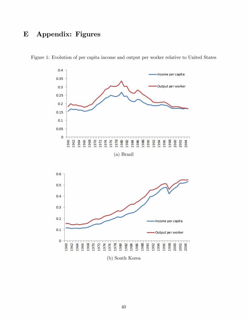
E Appendix: Figures

Figure 1: Evolution of per capita income and output per worker relative to United States

(a) Brazil

(b) South Korea

40

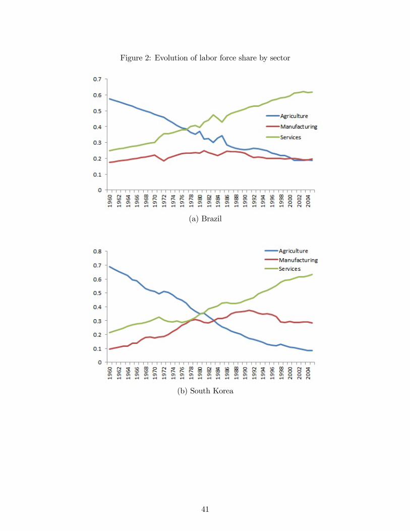
Figure 2: Evolution of labor force share by sector

(a) Brazil

(b) South Korea

41

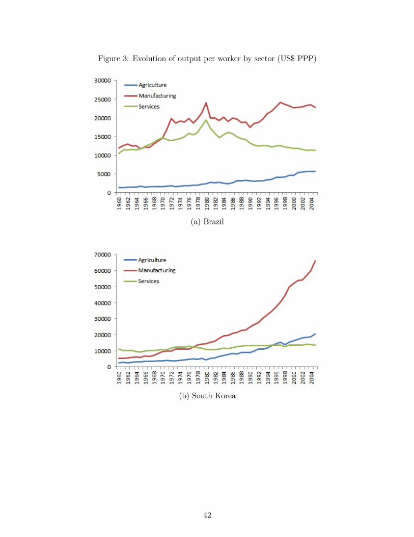
Figure 3: Evolution of output per worker by sector (US$ PPP)

(a) Brazil

(b) South Korea

42

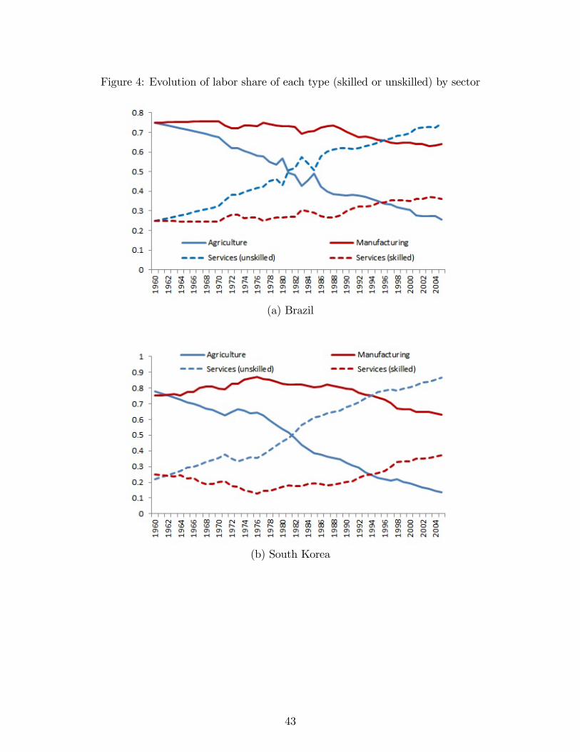
Figure 4: Evolution of labor share of each type (skilled or unskilled) by sector

(a) Brazil

(b) South Korea

43

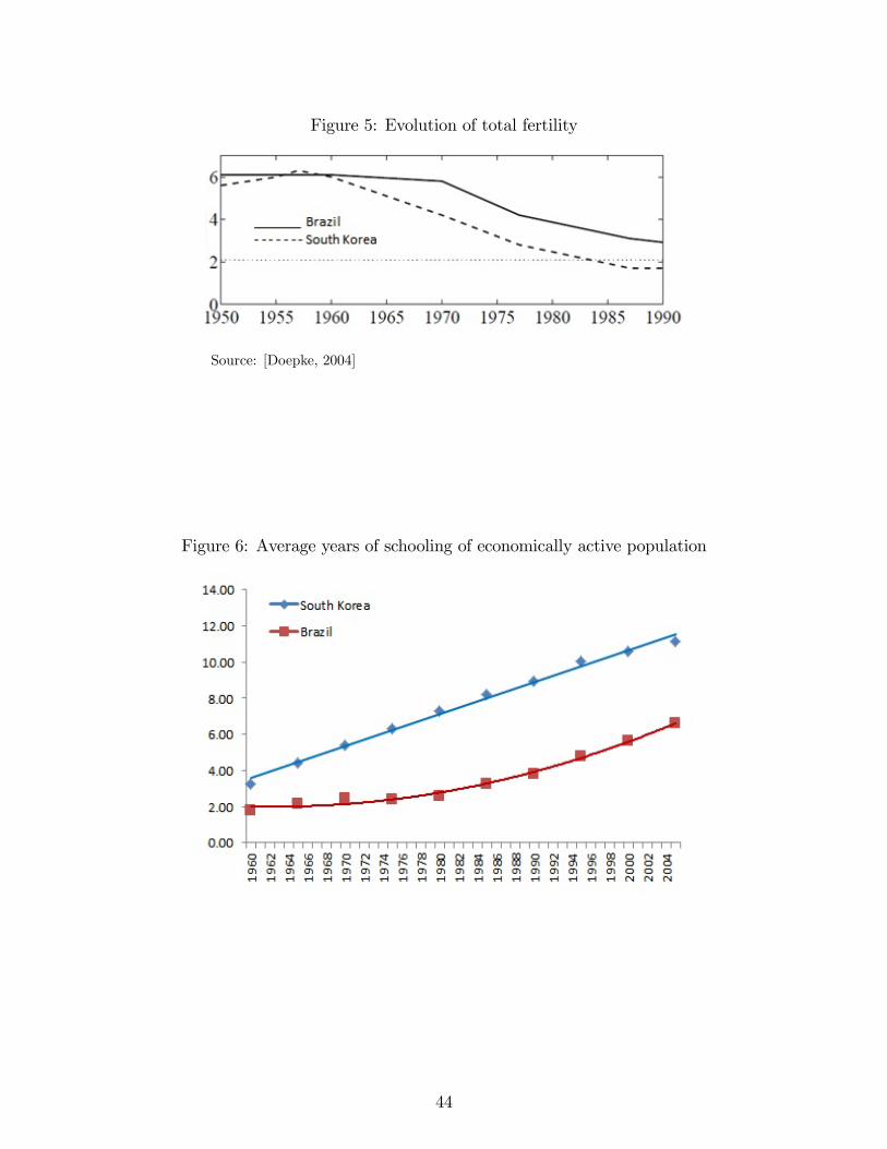
Figure 5: Evolution of total fertility

Source: [Doepke, 2004]

Figure 6: Average years of schooling of economically active population

44

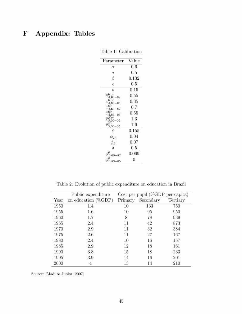
F Appendix: Tables

Table 1: Calibration

Parameter Value� 0.6� 0.5� 0.132� 0.5b 0.15

�cKorA;60�82 0.55�cKorA;83�05 0.35�cBrA;60�82 0.7�cBrA;83�05 0.55�cKorS;60�05 1.3�cBrS;60�05 1.6� 0.155�H 0.04�L 0.07� 0.5

�gL;60�82 0.069�gL;83�05 0

Table 2: Evolution of public expenditure on education in Brazil

Public expenditure Cost per pupil (%GDP per capita)Year on education (%GDP) Primary Secondary Tertiary1950 1.4 10 133 7501955 1.6 10 95 9501960 1.7 8 78 9391965 2.4 11 42 8731970 2.9 11 32 3841975 2.6 11 27 1671980 2.4 10 16 1571985 2.9 12 18 1611990 3.8 15 18 2331995 3.9 14 16 2012000 4 13 14 210

Source: [Maduro Junior, 2007]

45

Table 3: Adjusted enrollment ratios

Primary SecondaryYear Brazil Korea Brazil Korea1960 0.95 0.94 0.11 0.271965 1.0 1.0 0.16 0.351970 0.72 1.0 0.26 0.421975 0.88 1.0 0.26 0.561980 0.99 1.0 0.34 0.761985 1.0 0.96 0.35 0.951990 1.0 1.0 0.39 1.0

Source: [Doepke, 2004]

Table 4: Brazil: Percentage of population with highest level attained

Primary Secondary TertiaryYear No schooling Total Completed Total Completed Total Completed1960 56.00 36.75 15.71 5.97 3.62 1.21 1.101965 49.37 41.42 17.56 7.54 3.84 1.57 1.401970 42.50 46.00 19.40 9.60 3.70 2.00 1.701975 32.70 57.30 4.30 5.70 2.28 4.30 3.471980 32.90 55.30 4.90 6.90 2.90 5.00 3.691985 28.87 55.44 19.53 10.24 4.54 5.45 4.051990 24.99 54.88 27.04 14.18 6.66 5.94 4.351995 20.69 53.79 30.52 18.96 9.52 6.56 4.762000 17.75 49.54 30.44 25.35 13.85 7.30 5.252005 15.66 41.79 26.51 34.21 21.25 8.09 5.77

Table 5: South Korea: Percentage of population with highest level attained

Primary Secondary TertiaryYear No schooling Total Completed Total Completed Total Completed1960 56.90 29.60 26.20 10.90 5.80 2.60 1.881965 43.60 35.20 33.50 17.50 7.55 3.60 2.671970 34.30 38.10 26.50 21.80 9.90 5.70 4.291975 25.20 39.20 37.40 28.70 13.04 6.90 5.291980 19.70 34.50 33.04 36.90 18.70 8.90 6.581985 15.41 27.62 26.55 45.26 24.42 11.71 8.191990 14.22 24.35 23.43 41.86 25.14 19.57 12.671995 8.70 18.20 17.30 51.90 36.20 21.10 12.622000 7.45 14.79 14.21 50.90 35.98 26.82 14.752005 5.62 12.70 12.27 49.69 37.12 31.99 16.26

46

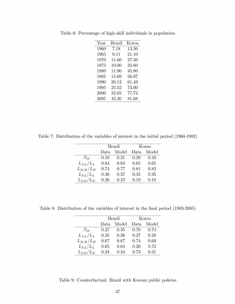
Table 6: Percentage of high-skill individuals in population

Year Brazil Korea1960 7.18 13.501965 9.11 21.101970 11.60 27.501975 10.00 35.601980 11.90 45.801985 15.69 56.971990 20.12 61.431995 25.52 73.002000 32.65 77.722005 42.30 81.68

Table 7: Distribution of the variables of interest in the initial period (1960-1982)

Brazil KoreaData Model Data Model

NH 0.10 0.31 0.29 0.49LA;L=LL 0.64 0.63 0.65 0.65LM;H=LH 0.74 0.77 0.81 0.82LS;L=LL 0.36 0.37 0.35 0.35LS;H=LH 0.26 0.23 0.19 0.18

Table 8: Distribution of the variables of interest in the �nal period (1983-2005)

Brazil KoreaData Model Data Model

NH 0.27 0.35 0.70 0.74LA;L=LL 0.35 0.36 0.27 0.28LM;H=LH 0.67 0.67 0.74 0.69LS;L=LL 0.65 0.64 0.26 0.72LS;H=LH 0.33 0.34 0.73 0.31

Table 9: Counterfactual: Brazil with Korean public policies

47

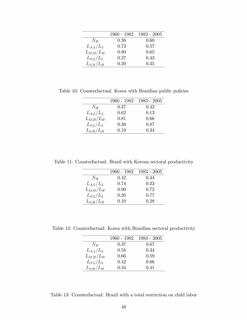
1960 - 1982 1983 - 2005NH 0.38 0.60

LA;L=LL 0.73 0.57LM;H=LH 0.80 0.65LS;L=LL 0.27 0.43LS;H=LH 0.20 0.35

Table 10: Counterfactual: Korea with Brazilian public policies

1960 - 1982 1983 - 2005NH 0.37 0.42

LA;L=LL 0.62 0.13LM;H=LH 0.81 0.66LS;L=LL 0.38 0.87LS;H=LH 0.19 0.34

Table 11: Counterfactual: Brazil with Korean sectoral productivity

1960 - 1982 1983 - 2005NH 0.42 0.44

LA;L=LL 0.74 0.23LM;H=LH 0.90 0.72LS;L=LL 0.26 0.77LS;H=LH 0.10 0.28

Table 12: Counterfactual: Korea with Brazilian sectoral productivity

1960 - 1982 1983 - 2005NH 0.37 0.67

LA;L=LL 0.58 0.34LM;H=LH 0.66 0.59LS;L=LL 0.42 0.66LS;H=LH 0.34 0.41

Table 13: Counterfactual: Brazil with a total restriction on child labor

48

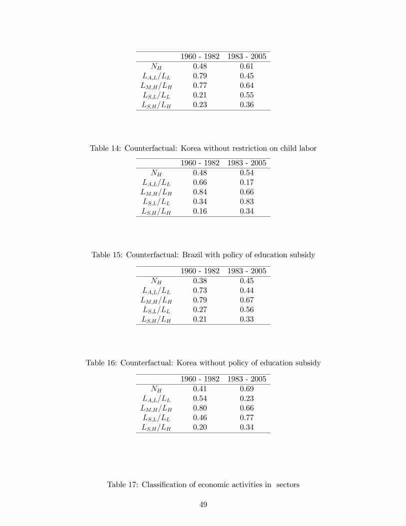
1960 - 1982 1983 - 2005NH 0.48 0.61

LA;L=LL 0.79 0.45LM;H=LH 0.77 0.64LS;L=LL 0.21 0.55LS;H=LH 0.23 0.36

Table 14: Counterfactual: Korea without restriction on child labor

1960 - 1982 1983 - 2005NH 0.48 0.54

LA;L=LL 0.66 0.17LM;H=LH 0.84 0.66LS;L=LL 0.34 0.83LS;H=LH 0.16 0.34

Table 15: Counterfactual: Brazil with policy of education subsidy

1960 - 1982 1983 - 2005NH 0.38 0.45

LA;L=LL 0.73 0.44LM;H=LH 0.79 0.67LS;L=LL 0.27 0.56LS;H=LH 0.21 0.33

Table 16: Counterfactual: Korea without policy of education subsidy

1960 - 1982 1983 - 2005NH 0.41 0.69

LA;L=LL 0.54 0.23LM;H=LH 0.80 0.66LS;L=LL 0.46 0.77LS;H=LH 0.20 0.34

Table 17: Classi�cation of economic activities in sectors

49

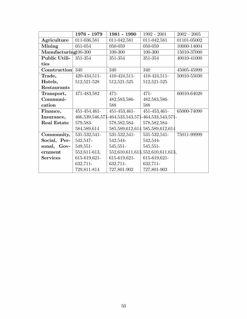
1976 - 1979 1981 - 1990 1992 - 2001 2002 - 2005Agriculture 011-036,581 011-042,581 011-042,581 01101-05002Mining 051-054 050-059 050-059 10000-14004Manufacturing100-300 100-300 100-300 15010-37000Public Utili-ties

351-354 351-354 351-354 40010-41000

Construction 340 340 340 45005-45999Trade,Hotels,Restaurants

420-434,511-512,521-528

410-424,511-512,521-525

410-424,511-512,521-525

50010-55030

Transport,Communi-cation

471-483,582 471-482,583,586-588

471-482,583,586-588

60010-64020

Finance,Insurance,Real Estate

451-454,461-466,539,546,571-579,583-584,589,614

451-453,461-464,533,543,571-578,582,584-585,589,612,614

451-453,461-464,533,543,571-578,582,584-585,589,612,614

65000-74090

Community,Social, Per-sonal, Gov-ernmentServices

531-532,541-542,547-549,551-552,611-613,615-619,621-632,711-729,811-814

531-532,541-542,544-545,551-552,610,611,613,615-619,621-632,711-727,801-902

531-532,541-542,544-545,551-552,610,611,613,615-619,621-632,711-727,801-903

75011-99999

50