edps 590bay carolyn j. anderson - college of education

Introduction to Bayesian Inference and ModelingEdps 590BAY

Carolyn J. Anderson

Department of Educational Psychology

c©Board of Trustees, University of Illinois

Fall 2019

Introduction What Why Probability Steps Example History Practice

Overview

◮ What is Bayes theorem

◮ Why Bayesian analysis

◮ What is probability?

◮ Basic Steps

◮ An little example

◮ History (not all of the 705+ people that influenceddevelopment of Bayesian approach)

◮ In class work with probabilities

Depending on the book that you select for this course, read eitherGelman et al. Chapter 1 or Kruschke Chapters 1 & 2.

C.J. Anderson (Illinois) Introduction Fall 2019 2.2/ 29


Main References for Course

Throughout the coures, I will take material from

◮ Gelman, A., Carlin, J.B., Stern, H.S., Dunson, D.B., Vehtari,A., & Rubin, D.B. (20114). Bayesian Data Analysis, 3rdEdition. Boco Raton, FL, CRC/Taylor & Francis.**

◮ Hoff, P.D., (2009). A First Course in Bayesian Statistical

Methods. NY: Sringer.**

◮ McElreath, R.M. (2016). Statistical Rethinking: A Bayesian

Course with Examples in R and Stan. Boco Raton, FL,CRC/Taylor & Francis.

◮ Kruschke, J.K. (2015). Doing Bayesian Data Analysis: A

Tutorial with JAGS and Stan. NY: Academic Press.**

** There are e-versions these of from the UofI library. There is averson of McElreath, but I couldn’t get if from UofI e-collection.



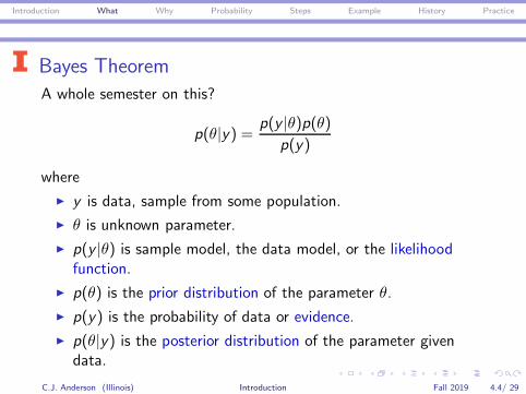
Bayes Theorem

A whole semester on this?

p(θ|y) =p(y |θ)p(θ)

p(y)

where

◮ y is data, sample from some population.

◮ θ is unknown parameter.

◮ p(y |θ) is sample model, the data model, or the likelihoodfunction.

◮ p(θ) is the prior distribution of the parameter θ.

◮ p(y) is the probability of data or evidence.

◮ p(θ|y) is the posterior distribution of the parameter givendata.



Why Bayes?

◮ Probabilities can numerically represent a set of rational beliefs(i.e., fundamentally sound and based on rational rules).

◮ Explicit relationship between probability and information.

◮ Quantifies change in beliefs of a rational person when givennew information (i.e., uses all available information–past &present).

◮ Very flexible

◮ Common sense interpretations.

In other words, if p(θ) approximates our beliefs, then p(θ|y) isoptimal to what our posterior (after we have new information)beliefs about θ should be. Bayes can be used to explore how beliefsshould be up-dated given data by someone with no information(e.g., who will win the 2020 presidental election?) or with someinformation (e.g., will is rain in Champaign in 2019?).C.J. Anderson (Illinois) Introduction Fall 2019 5.5/ 29


General Uses of a Bayesian Approach

◮ Parameter estimates with good statistical properties

◮ Parsimonious descriptions of observed data.

◮ Predictions for missing data.

◮ Predictions of future data.

◮ Computational frame-work for model estimation andvalidation.

◮ Provides a solution to complicated statistical problems thathave no obvious (non-Bayesian) method of estimation andinference (e.g., complex statistical model, estimation of rareevents).



Major Problems using Bayesian Approach

◮ Specifying prior knowledge; that is, choosing a prior.

◮ Sample fromp(y |θ)p(θ)

p(y)

◮ Computationally intensive



What do we Mean by “Probability”Different authors of Bayesian texts use different terms forprobability, which reflect different conceptualizations.

◮ Beliefs

◮ Credibility

◮ Plausibilities

◮ Subjective

There are multiple specific definitions:

◮ Frequentist: long run relative frequency of an event.

◮ Bayesian: a fundamental measure of uncertainty that followrules probability theory.

◮ What is the probability of thunder snow tomorrow?◮ What is the probability that Clinton nuclear power plant has a

melt down?◮ What is the probability that a coin tossed lands on head?



Probabilities as We’ve Known Them

Probabilities are foundational concept!Probabilitiesare numerical quantities that measures of uncertainty.

Justification for the statement “The probability that an evennumber comes up on a toss of a dice equals 1/2.”

Symmetry or exchangeability argument:

p(even) =number of evens rolled

number of possible results

The justification is based on the physical process of rolling a dicewhere we assume each side of a 6 sided die are equal likely, threesides have even numbers, the other three have odd numbers.

y1 =even or odd on first roll should be the same as y2 on 2nd, etc.



Probabilities as We’ve Known ThemAlternative justification for the statement “The probability that aneven number comes up on a toss of a dice equals 1/2.”

Frequency argument:

p(even) = Long run relative frequency

Long (infinite) sequence of physically independent rolls of the dice.

Are these justifications subjective? These involve hypotheticals:physical independence, infinite sequence of rolls, equally likely,mathematical idealizations.

How would either of these justifications apply to

◮ If we only roll dice once?

◮ What’s the probability that USA womens soccer team winsthe next World Cup?



Probabilities as measure of Uncertainty

◮ Randomness creates uncertainty and we already do it incommon speech...what are synonyms for “probability”?

◮ Coherence: probabilities principles of basic axioms ofprobability theory, which have a consequences things such as :

◮ 0 ≤ p(X) ≤ 1◮ if X is subset or equal to Y , then p(X ) ≤ p(Y )◮

∑p(X ) = 1 or

∫p(X ) = 1 item

p(X ,Y ) = p(X ) + p(Y )− p(X⋂Y )



Expected Value◮ Expected value is a mean of some statistic or quantity based

on a random event or outcome.◮ For discrete random variables, say X with “probability mass

function” p(x), the mean of X is

E (X ) = µX =

I∑i=1

xiPr(X = xi),

where I is the number of possible values for x , andPr(X = xi ) is the probability that X = xi .

◮ For continuous random variables, say X with a probabilitydensity function f (x), the mean of X is

E (X ) = µX =

∫x

xf (x)d(x),

where integration is over all possible values of x .



Basic Steps of Bayesian Analysis(from Gelman et al.)

I assume that you have research questions, collected relavent data,and know the nature of the data.

◮ Set up full probability model (a joint probability distributionfor all observed and unobserved variables that reflectknowledge and how data were collected):

p(y , θ) = p(y |θ)p(θ) = p(θ|y)p(y)

This can be the hard part◮ Condition on data to obtain the posterior distribution:

p(θ|y) = p(y |θ)p(θ)/p(y)

Tools: analytic, grid approximation, Markov chain MonteCarlo (Metropolis-Hastings, Gibbs sampling, Hamiltonian).

◮ Evaluate model fit.C.J. Anderson (Illinois) Introduction Fall 2019 13.13/ 29


A Closer Look at Bayes RuleI am being vagues in terms of what y and θ are (e.g., continuous,discrete, number of parameters, what the data are).

p(θ|y) =p(y |θ)p(θ)

p(y)

∝ p(y |θ)p(θ)

where p(y)

◮ ensures probability sums to 1.

◮ is constant (for a given problem).

◮ “average” of numerator or the evidence.

◮ For discrete y : p(y) =∑

θ∈Θ p(y |θ)p(θ)

◮ For continuous y : p(y) =∫θp(y |θ)p(θ)d(θ)



More on the Uses of a Bayesian Approach

◮ If p(θ) is wrong and doesn’t represent our prior beliefs, theposterior is still useful. The posterior, p(θ|y), is optimal underp(θ) which means that p(θ|y) will generally serve as a goodapproximation of what our beliefs should be once we havedata.

◮ Can use Bayesian approach to investigate how data would beupdated using (prior) beliefs from different people. You canlook at how opinions may changes for someone with weak

prior information (vs someone with strong prior beliefs). Oftendiffuse or flat priors are used.

◮ Can handle complicated problems.



Example: Spell Checker

(from Gelman et al.)

Suppose the word ”radom” is entered and we want to know theprobability that this is the word intended, but there 2 other similarwords that differ by one letter.

frequencyfrom Google’sGoogle Prior model numerator

θ database p(θ) p(‘radom’|θ) p(θ)p(‘radom’|θ)

random 7.60 × 10−5 0.9227556 0.001930 1.47 × 10−7

radon 6.05 × 10−6 0.0734562 0.000143 8.65 × 10−10

radom 3.12 × 10−7 0.0037881 0.975000 3.04 × 10−7

total 8.2362 1.00 1.00 4.51867×10−5 ×10−7



Spell Checker (continued)

Google’s numeratorPrior model of Bayes Posterior

θ p(’radom’) p(‘radom’|θ) p(θ)p(‘radom’|θ) p(θ|‘radon’)

random 0.9227556 0.001930 1.47 × 10−7 0.325radon 0.0734562 0.000143 8.65 × 10−10 0.002radom 0.0037881 0.975000 3.04 × 10−7 0.673

total 1.00 1.00 4.51867 × 10−7 1.000



Spell Checker (continued)

DataPrior model Posterior

θ p(θ) p(‘radom’|θ) p(θ|‘radon’)

random 0.9227556 0.001930 0.325radon 0.0734562 0.000143 0.002radom 0.0037881 0.975000 0.673

total 1.00 1.00 1.000

What is “radom”?

Some averaging of prior and data going on...most in this nextlecture.

What could be some criticisms of this example or how might it beimproved?



History: Rev Thomas Bayessources: Leonard (20140, Fienberg, S. (2006).



1700sKeep in mind that statistics is a relatively newer field (only about250 years old).

◮ 1763 Rev Thomas Bayes gave the first description of thetheorem in “An essay toward solving a problem in the doctrineof chance”. This published posthumously by Richard Price.

◮ Bayes dealt with the problem of drawing inference; that is,concerned with “degree of probability”.

◮ Bayes introduces uniform prior distribution for binomialproportion.

◮ Price added an appendix that deals with the problem ofprediction.

◮ Bayes did not give statement of what we call “Bayes Theorem”.◮ 1749 David Hartley’s book describes the “inverse” result and

attributes is to a friend. Speculation is that the friend waseither Saunderson or Bayes.



1700s (continued)

◮ 1774 Pierre Simon LaPlace gave more elaborate version ofBayes theorem for the problem of inference for an unknownbinomial probability in more modern language. He clearlyaugured for choosing a uniform prior because he reasoned thatthe posterior distribution of the probability should beproportional to the prior,

f (θ|x1, x2, . . . xn) ∝ f (x1, x2, . . . , xn|θ)

I think this is why the term “inverse probability” was used.

◮ LaPlace introduced the idea of “indifference” as an argumentto use uniform prior; that is, you have no information whatthe parameter should be.

◮ I.J. Bienayme generalized LaPlace’s work.

◮ von Mise gave a rigorous proof of Bayes theorem.



1800s

1837–1843: at least 6 authors, working independently, madedistinctions between probabilities of things (objective) andsubjective meaning of probability (i.e., S.D. Poisson, D. Bolzano,R.L Ellis, J.F. Frees, J.S. Mills and A.A. Counot).

Debate on meaning of probability continued throughout the 1800s.

Some adopted the inverse probability (i.e, Bayesian) but alsoargued for a role of experience, including Pearson, Gosset andothers.



1900s

◮ 1912–1922: Fisher advocated moving away from inversemethods toward inference based on likelihood.

◮ Fished moved away from “inverse probability” and argued fora frequentist approach.

“. . . the theory of inverse probability is founded upon an error,and must wholly be rejected.”

◮ Fundamental change in thinking.

◮ Beginnings of formal methodology for significance tests.

◮ J Neyman & Ego Pearson gave more mathematical detail andextended (“completed”) Fisher’s work which gave rising to thehypohthesis test and confidence intervals



1900s (continued)

◮ After WWWI, frequentist methods usurped inverse probabilityand Bayesian statistician were marginalized.

◮ R. von Mises justified the frequentist notion of probability;however, in 1941 he used a Bayesian argument to critiqueNeyman’s method for confidence intervals. He argued thatwhat really is wanted was posterior distribution.

◮ 1940 Wald showed that Bayesian approach yielded goodfrequentist properties and helped to rescue Bayes Theoremfrom obscurity.

◮ 1950s The term “frequentist” starts to be used. The term“Bayes” or “Bayes solution” was already in use. The term“classical” statistics refers to the frequentist.



1900s (continued)

◮ J.M Keynes (1920s) laid out axiomatic formulation and newapproach to subjective probabilities via the concept of expectutility. Some quotes that reflect this thinking:

◮ “In the long run we are all dead.”◮ “It is better to be roughly right than precisely wrong.”◮ “When the facts change, I change my mind.”

◮ 1930s: Bruno de Finetti gave a different justification forsubject probabilities and introduced the notion of“exchangeability” and implicit role of the prior distribution.

◮ Savage build on de Finetti’s ideas and developed set of axiomsfor non-frequentist probabilities.



WWWII

◮ Alan Turing and his code breaking work was essentiallyBayesian — sequential data analysis using weights of evidence.It is thought that he independently thought of these ideas.

◮ Decision-theory developments in the 1950s.



1980s and Beyond

Large revival started in the late 1980s and 1990s. This was due tonew conceptual appoarches and lead to rapid increases inapplications. The increase in computing power helped fuel this.

Non-Bayesian approaches will likely remain important because ofthe hight computational demand and expense of Bayeisan methods,even though there are continual developments in computing power.



Practice 1: Subjective ProbabilityDiscuss the following statements:“The probability of event E isconsidered ‘subjective’ if two rational people A and B can assignunequal probabilities to E, PA(E ) and PB(E ). These probabilitiescan also be interpreted as ‘conditional’: PA(E ) = P(E |IA) andPB(E |IA), where IA and IB represent the knowledge available toperson A and B , respectively.” Apply this idea to the followingexamples.

◮ The probability that a “6” appears when a fair die is rolled,where A observes the outcome and B does not.

◮ The probability that USA wins the next mens World Cup, whereA is ignorant of soccer and B is a knowledgable sports fan.

◮ The probability that UofI’s football team goes to a bowl game,where A is ignorant of Illini football and B is knowledgable ofIllini football.



Practice 2: Conditional Probabilities and a little R(from Gelman et al.)Suppose that θ = 1, then Y has a normal distribution with mean 1and standard deviation σ, and if θ = 2 then Y is normal with mean2 and standard deviation σ. Also suppose Pr(θ = 1) = 0.5 andPr(θ = 2) = 0.5.

◮ For σ = 2, write the formula for the marginal probabilitydensity for y and sketch/plot it. For the graphr, you will needto use the R commands:

◮ seq◮ dnorm◮ plot

◮ What is Pr(θ = 1|y = 1) and what is Pr(θ = 1|y = 2). (hint:Definition of conditional probability, Bayes Theorem)

◮ Describe how the posterior density of θ in shape as◮ σ increases◮ σ decreases◮ Difference between µ’s increase.◮ Different between µ’s decrease.


edps 590bay carolyn j. anderson - college of education

Documents