edges in models of shear flow - university of...

Under consideration for publication in J. Fluid Mech. 1

Edges in Models of Shear Flow

Norman LebovitzUniversity of Chicago

andGiulio Mariotti

Boston University

(Received )

A characteristic feature of the onset of turbulence in shear flows is the appearance of an“edge,” a codimension-one invariant manifold that separates “lower” orbits, which decaydirectly to the laminar state, from “upper” orbits, which decay more slowly and lessdirectly. The object of this paper is to elucidate the structure of the edge that makes thisbehavior possible. To this end we consider a succession of low-dimensional models. In do-ing this we isolate geometric features that are robust under increase of dimension and aretherefore candidates for explaining analogous features in higher dimension. We find thatthe edge, which is the stable manifold of a “lower-branch” state, winds endlessly aroundan “upper-branch” state in such a way that upper orbits are able to circumnavigate theedge and return to the laminar state.

1. Introduction

The Navier-Stokes (NS) equations may be viewed as a dynamical system of infinitedimension. This is a view that has seen some remarkable successes in the problem ofturbulence in shear flows (Eckhardt (2008), Waleffe (1997)). The latter problem is ap-proached theoretically by considering first a laminar shear flow (plane Couette flow, pipeflow, etc.) and its stability as the Reynolds number R is increased. What distinguishesthe problem of shear flow from other hydrodynamic problems – and indeed from manyother problems in applied mathematics – is that the onset of the turbulent or disorderedstate is not accompanied by an instability of the laminar flow. This places particularimportance on understanding the nature of the boundary of the basin of attraction ofthe stable, laminar state and how it changes with R. This boundary is an invariant setand, at least in straightforward examples, is of codimension one.

For sufficiently small values of R, the laminar flow is the only steady state and it isglobally stable: all perturbations die out (i.e., relaminarize). When R exceeds a criticalvalue RSN additional steady states may appear and it can no longer be strictly truethat all perturbations relaminarize. It nevertheless continues to be true that relaminar-ization is ubiquitous: almost all orbits die out. Exceptions are those lying on a certaincodimension-one invariant manifold, called an edge (Duguet et al. (2008), Vollmer et al.

(2009)), and separating orbits that die out quickly from orbits that die out slowly. Theedge is in many examples the stable manifold of an “edge state” which may take one ofa number of forms (e.g., an equilibrium point, a periodic orbit, a chaotic saddle, . . .).A pair of relaminarizing orbits may originate extremely close to one another, one justbelow the edge (a lower orbit) and the other just above (an upper orbit). Orbits on theedge cannot relaminarize as they tend, not to the laminar point, but to the edge state.

Is this edge the basin boundary? There is a convention involved in answering thisquestion. Intuitively a boundary separates one region from another whereas the edge

2 Norman Lebovitz University of Chicago and Giulio Mariotti Boston University

merely separates one part of the basin of attraction from another part of the sameregion. However, a widely accepted mathematical definition of the boundary ∂S of a setS ∈ Rn is:

∂S consists of points x ∈ Rn such that any neighborhood of x contains both pointsthat are in S and points that are not in S.

Under this definition edge points are indeed points of the basin boundary, and we adoptthis convention here (see also Lebovitz (2012)).

The issue addressed in this paper is that of the geometric structure of the edge. Thisquestion has been raised before in the specific form: how do upper orbits relaminarize? Itarises because familiar pictures of basin boundaries present obstacles to relaminarization(see the discussion in Vollmer et al. (2009)). For example, if one envisages the edge as aspherical surface surrounding the laminar point, an upper orbit would have to penetratethis surface to relaminarize, and this is not possible since the surface is an invariant set.If the edge is rather like a plane, it could not be a complete plane separating phase spacefor the same reason. If the edge of either of these examples is replaced by a subset of itself,it would have a boundary and this would likewise be an invariant set which one shouldbe able to identify in the dynamics. These questions have led to speculations regardingthe structure of the edge (Skufca et al. (2006)). In the spirit that we are unlikely tounderstand that structure in the infinite-dimensional case if we do not understand it inthe finite-dimensional case, we consider the latter in this paper.

In the context of the low-dimensional models discussed here, we find a consistentpicture of the edge and relate it to familiar invariant sets. We study it in a succession ofdynamical systems of increasing dimension. The strategy is to isolate properties of theedge that are common to them all since we then have grounds to speculate that theseproperties generalize to higher – perhaps infinite – dimension.

There are three principal sections, bracketed by preliminaries (§2) and a discussion (§6)containing a distillation of the detailed information obtained in studying the models of§§3, 4 and 5. In §3 we recapitulate results previously obtained for a two-dimensional model(Lebovitz (2012)) and present a cartoon generalization of it to a three-dimensional modelwhich turns out to contain, in a relatively simple setting, the principal structures of thebasin boundary found in the higher-dimensional models. We consider a well-known fourdimensional model of Waleffe in §4 and investigate the structure of the edge, indicatingits extent and complexity. §5 is devoted to a six-dimensional model for which the basinboundary has a strong family resemblance to those of the lower-dimensional modelsdespite differences of detail.

2. Preliminaries

Suppose that the shear flow under investigation is described by the velocity field U ,and that the NS equations are modified by subtracting U from the total velocity. Thishas the effect that the unperturbed flow is then represented by the solution u = 0 ofthe modified NS equations. If a fixed set of n basis functions – satisfying the boundaryconditions and the condition of incompressibility – is then chosen and used for a Galerkinprojection of these modified equations, one finds

dx

dt= Ax + b(x), x ∈ Rn (2.1)

where the ith component xi of the vector x is the coefficient of the ith basis function.The matrix A and the nonlinear term b inherit features of the full problem. The matrix

Edges in Models of Shear Flow 3

A is stable (i.e., all its eigenvalues have negative real parts), and it is non-normal. Theseconditions taken together imply that, while all solutions of the linearized problem dieout (or relaminarize), some of them may undergo a large-amplitude transient beforerelaminarizing. The amplitude of this transient is found to increase with R. This is ageneral feature of shear flows (cf. Butler & Farrell (1992)). The nonlinear term b isquadratic in x, reflecting the quadratic nonlinearity of the NS equations. Moreover, onefinds (x, b(x)) = 0 where (, ) denotes the inner product, reflecting conservation of energyof the corresponding Euler equations.

In earlier studies (Lebovitz (2009), Lebovitz (2012)) emphasis was placed on discover-ing the emergence of an edge via a homoclinic bifurcation as parameters change. Since inthe present paper it is the structure of the edge we wish to study, we restrict considerationto parameter regimes in which the edge is already present.

Much of the description found below depends on relating various invariant sets andmanifolds to one another. We use standard notations like O,Xlb,Xub to denote equi-librium points, and B,SM,UM to denote the invariant sets Basin of attraction, StableManifold, Unstable Manifold, respectively. Thus B(O) is the basin of attraction of theorigin, ∂B(O) is its boundary, SM(Xlb) is the stable manifold of the point Xlb, etc.

3. Lowest Dimensions

In this section we consider a two-dimensional and a three-dimensional model. Eachis of the shear-flow type of equation (2.1) but no further claim beyond that is maderegarding their faithfulness to the shear-flow problem.

3.1. A two-dimensional model

We begin with a model introduced in Lebovitz (2012):

x1 = −δx1 + x2 + x1x2 − 3x2

2, x2 = −δx2 − x2

1+ 3x1x2, δ = 1/R. (3.1)

We summarise some of its features as studied in Lebovitz (2012).The critical value below which the origin is globally, asymptotically stable is RSN = 2.

There a saddle-node bifurcation occurs and for larger values of R there are, in additionto the origin, two further equilibrium points: the lower-branch equilibrium point Xlb andthe upper-branch equilibrium point Xub. Of these Xub is initially stable whereas Xlb isunstable for all R > RSN , with a one-dimensional stable manifold and a one-dimensionalunstable manifold, indicated by SM and UM in Figure 1. The stability properties ofXub change when R = 2.5 where a Hopf bifurcation takes place so we consider a smallervalue (we use R = 2.45 as an example) for which Xub is stable and a larger value (weuse R = 2.55) for which it is unstable with a complex-conjugate pair of eigenvalues.

The qualitative properties of ∂B(O), the boundary of the basin of attraction of theorigin change only slightly under this change of R, and may be described as follows.• R = 2.45: We call attention to SM(Xlb), the stable manifold of Xlb, denoted by

SM in Figure 1. It consists of two orbits tending to Xlb as t → ∞. As t → −∞, theright-hand orbit is unbounded, whereas the left-hand orbit winds around the periodicorbit P and therefore remains in a bounded region of phase space. It is clear that ∂B(O)is the union of two sets:

∂B(O) = SM(Xlb) ∪ P. (3.2)

The periodic orbit P separates points in B(O) from points in B(Xub), the basin ofattraction of Xub, and therefore clearly forms one part of the boundary of B(O) (calleda “strong” part in Lebovitz (2012)). SM(Xlb) does not separate B(O) from any other

4 Norman Lebovitz University of Chicago and Giulio Mariotti Boston Universityx

2

x1

R=2.45

Xlb

UM

SM

XubP

O

x2

x1

R=2.55

O

XlbSM

UM

Xub

Figure 1. In the left-hand figure, the left-hand arc of the stable manifold SM of Xlb windsaround a periodic orbit P , which is itself the boundary of the basin of attraction of Xub; ∂B(O)is the union of two invariant manifolds, SM(Xlb) and P . In the right-hand figure Xub is nowunstable and ∂B(O) is the union of SM(Xlb) with the point Xub.

set: it merely separates orbits in B(O) with one kind of evolution from orbits in B(O)with a different kind of evolution. Therefore SM(Xlb) is an edge (or a “weak” part ofthe boundary, as defined in Lebovitz (2012)).Consider the open set bounded by UM(Xlb) (online, the red curves in Figure 1) togetherwith the laminar point O. Modify it by excluding the point Xub. Any orbit beginning ata point in this modified region, when integrated backwards in time, tends to P . Thus thisbounded, two-dimensional region is UM(P ). Furthermore, there is one orbit in UM(P )which tends (as t → +∞) to Xlb, i.e., while UM(P ) and SM(Xlb) are not the same,they have a nontrivial intersection consisting of the left-hand arc of SM(Xlb). This is abounded orbit and its α-limit set is precisely P .

• R = 2.55. The stabilty of Xub ceases at R = 2.5 and with it its basin of attractionand the periodic orbit P . Now

∂B(O) = SM(Xlb) ∪ {Xub} (3.3)

and consists solely of an edge: all orbits in the plane except those lying on ∂B(O) relam-inarize.The set UM(Xub) has essentially the same description as that of UM(P ) for the caseR = 2.45 above. Again there is a single orbit, the left-hand arc of SM(Xlb), representingthe intersection UM(Xub) ∩ SM(Xlb). The α-limit set of the left-hand arc of SM(Xlb)is now the (unstable) equilibrium point Xub.It is clear that orbits beginning on one side of SM(Xlb) undergo a different evolutionfrom those beginning on the other side. Orbits beginning in the windings around Xub

may persist for a long time before relaminarizing.

3.2. A three-dimensional generalization

The proceeding provides an understandable model of an edge state, but two-dimensionaldynamical systems have special properties which may fail to generalize to higher-dimensionalsystems. As a first pass at trying to understand what may happen in such generalizations,


O

UM(Xub) ∩ SM(Xlb)

x1

x2

x3

Xub

Xlb

SM(Xlb)

Figure 2. SM(Xlb) is now two-dimensional and forms the edge. UM(Xub) is likewise twodimensional and has a one-dimensional intersection with SM(Xlb).

we augment the system (3.1) with the single equation

x3 = −x3. (3.4)

The resulting equations continue to conform to the pattern of equation (2.1) above. Anyof the three equilibrium points (a1, a2) of the system (3.1) with (say) R = 2.55 becomesan equilibrium point (a1, a2, 0) of the three-dimensional model. Building a cartoon onthis model, we arrive at the Figure (2). Note that if we had considered the case R = 2.45instead, the cartoon diagram would include the periodic orbit P as well, now lying in theplane x3 = 0.

In this figure SM(Xub) is now the x3 axis. UM(Xub) is the same as in the two-dimensional model: it is a bounded, two-dimensional region lying in the x1x2 plane,and it intersects SM(Xlb) along a single curve (online, the green curve in Figure 2). The“folds” of the spiraling orbit of the two-dimensional system have become two-dimensional“scrolls” parallel to the x3 axis, and the flow through a generic point near Xub is nowtrapped for a time within these scrolls, ultimately relaminarizing. The same generalpicture holds in the case R = 2.45 except that the scrolls wind up, not on a straight linethrough Xub but on the cylinder parallel to the x3-axis and containing the periodic orbitP . The stable manifold of P is bounded by this cylinder; it forms the boundary of thebasin of attraction of Xub.

In both the two- and three-dimensional models, most orbits do not get particularlyclose to Xlb: only those beginning very close to SM(Xlb) do that. Two points very neara fold (or scroll) of SM(Xlb) but on opposite sides of it pass close to Xlb but mustcontinue to lie on opposite sides of SM(Xlb), and therefore have final evolutions towardO that are quite different. Moreover, orbits that begin between inner folds (or scrolls)must first wind their way out before approaching Xlb and may for this reason have verylong lifetimes.

We pass on now to a model adhering more closely to the fluid dynamics.


4. Waleffe’s Four-Dimensional Model

The four-dimensional model proposed in Waleffe (1997) – hereinafter W97 – adherescloser to the shear-flow problem in that its derivation is guided by Galerkin projectiononto modes believed to be decisive for the nonlinear development of (in this case) planeCouette flow. When shifted so as to make the origin of coordinates correspond to theunperturbed, laminar state, W97 takes the form

x1 = −δr1x1 − σ2x2x3 + σ1x2

4,

x2 = −δr2x2 + σ2x3 + σ2x1x3 − σ4x2

4,

x3 = −δr3x3 + σ3x2

4, (4.1)

x4 = − (σ1 + δr4) x4 + x4 (σ4x2 − σ3x3 − σ1x1) .

Here δ = 1/R represents the reciprocal of the Reynolds number, whereas the coefficientsσi, ri, i = 1, . . . , 4 are positive numbers derived via Waleffe’s Galerkin procedure. In thispaper the values of the σ’s and the r’s are taken to be

(σ1, σ2, σ3, σ4) = (0.31, 1.29, 0.22, 0.68),

(r1, r2, r3, r4) = (2.4649, 5.1984, 7.6729, 7.1289).

They correspond (approximately) to the wavenumber values

α = 1.30, γ = 2.28. (4.2)

These are (approximately) the values adopted in other studies of this system such as thoseof Dauchot & Vioujard (2000) (where slight numerical discrepancies from those foundhere are attributable to correspondingly small differences adopted for these parameters)and Cossu (2005).

The system (4.1) possesses the symmetry S = diag(1, 1, 1,−1). The hyperplane x4 = 0is therefore an invariant plane. It is not difficult to show that this plane lies in the basinof attraction of the origin. Since orbits cannot cross it, any structure made up of orbits,like other invariant sets, lie in one or another of the two regions x4 > 0 and x4 < 0. Weconfine our attention to the region x4 > 0, bearing in mind that any structures we findthere are duplicated in the region x4 < 0.

4.1. Equilibrium points

The origin of coordinates is an asymptotically stable equilibrium point and therefore hasa basin of attraction B = B(O).

The transition from the purely laminar toward more complicated behavior is governedby the existence and the structure of the boundary of B. These are intimately connectedwith Xlb and Xub, the lower- and upper-branch equilibrium points (Figure 3), and wenow turn to an examination of these.

4.1.1. The lower branch

This branch of equilibrium points has uniform stability properties: one unstable andthree stable eigenvalues for all values of R > RSN . There is accordingly a three-dimensionalstable manifold SM(Xlb) and a one-dimensional unstable manifold UM(Xlb). As dis-cussed more fully below (§4.2), SM(Xlb) is the edge, and the two arcs of UM(Xlb) bothlead, via different paths, to O.

4.1.2. The upper branch

This branch undergoes a change in its stability properties at P2. From the outset atSN to the nearby point P1, it is unstable with a complex pair of eigenvalues with negative


0.55

0.6

0.65

0.7

0.75

0.8

0.85

0.9

100 110 120 130 140 150

||y||

R

P1SN

P2

Upper branch

Lower branch

Figure 3. This shows the diagram of the norms of equilibrium solutions against the Reynoldsnumber R. For the chosen values of parameters in W97 there is a saddle-node bifurcation atRSN = 106.1393. Changes in the eigenvalues at the upper branch equilibrium point occur asindicated in the text, at the values RP1

= 106.2401 and RP2= 139.73738. The laminar solution

‖y‖ = 0 (not shown) is stable for all values of R.

real part and two real, positive eigenvalues. It remains unstable at P1 but the positive realroots coalesce and become a complex pair with a positive real part. At P2 this positivereal part passes through zero and, for larger values of R, is negative. The upper branchtherefore becomes and remains stable for R > RP2

.The bifurcation at P2 is of the Hopf type and is therefore accompanied by the birth

of a periodic orbit P . This orbit would be stable if it existed for R < RP2, but it

appears (on numerical evidence) that the new periodic orbit exists for R > RP2and

is therefore unstable. Since each upper-branch equilibrium point Xub is asymptoticallystable if R > RP2

, Xub has its own basin of attraction, which we will call D = B(Xub) todistinguish it from the principal object of study B = B(O). We have numerical evidencethat the unstable periodic orbit P lies on ∂D and, in fact, that the stable manifold of Pcoincides with ∂D.

The structure of solutions near Xub is important for understanding the edge becauseit is the winding up of the latter around Xub (for R < RP2

) or around D = B(Xub) (forR > RP2

) that allows orbits from both sides of the edge to relaminarize.

4.2. The structure of ∂B

We first observe the edge character of the stable manifold of Xlb by checking the orbitsbeginning ‘just above’ and ‘just below’ Xlb for some values of R. By ‘just above’ wewill mean initial values of x for which x4 is slightly greater than Xlb4, and by ‘justbelow’ initial values of x for which x4 is slightly smaller than Xlb4, whereas xi = Xlbi fori = 1, 2, 3 in both cases. Starting for values of R just greater than RSN , we find that allorbits, whether starting above or below, relaminarize. Those starting above take longer.We have done this for a large number of values of R, up to R = 10, 000, and find thatthis holds without exception.

We next construct parts of SM(Xlb) by a continuation method, starting at x = Xlb.


-0.1

0

0.1

0.2

0.3

0.4

0.5

0.6

-3 -2.5 -2 -1.5 -1 -0.5 0

x 4

x1

R=135x2=Xub2,x3=Xub3

’Xlb’

Xuboutermost fold

second fold

third fold

Figure 4. The stable manifold of Xlb winds around Xub infinitely often, producing a successionof three-dimensional folds. In this slice (the x4 − x1 slice passing through Xub) the outermostfold appears to be unbounded both to the left and the right (the other folds are bounded andappear as closed curves in this view). Single quotes around Xlb indicate that the latter fails tolie in the chosen hyperplane but is projected onto it.

The parts that are constructed are the intersections of SM(Xlb) with various hyperplanes,as indicated in the figures. In these figures, in order to emphasize the nature of SM(Xlb)near the other equilibrium point Xub, the hyperplanes are chosen to pass through thispoint.

Whereas SM(Xlb) cannot, by its definition, belong to B, it can and does belong to ∂B.Indeed, it seems that SM(Xlb) = ∂B for some values of R. This is so for R < RP2

≈ 139.7and we investigate an example of this (R = 135) first.

4.2.1. R=135

In this case ∂B consists of the union of SM(Xlb) with the single point Xub. Theintersection of this set with the hyperplane x2 = Xub2, x3 = Xub3 is shown in Figure 4.

Points on any of these folds tend, under the flow, toward Xlb as t → ∞. For example,a point starting on the third fold, after making two loops about Xub, then tends towardXlb. Higher-order folds (not shown) get arbitrarily close to Xub, and orbits originatingon them make more loops (and require more time), before tending toward Xlb. A pointvery close to a fold – but not exactly on it – will generate an orbit coming very close toXlb, but will then tend to O along one of the arcs of UM(Xlb): its final descent to Owill therefore depend on which side of the fold it originated from. The similarity withthe two-dimensional case (Figure 1, R = 2.55) is clear.

However, the outermost fold of Figure 4 appears to extend indefinitely in the ±x1

directions whereas, in order for the picture of an edge obtained from the two-dimensionalmodel to persist, there must be lines in phase space along which all folds are bounded atleast on one side. We therefore investigate a second slice through Xub but in a differenthyperplane (Figure 5). Here we find indeed that SM(Xlb) is bounded in the +x3 direction.

We next investigate the case when R = 145 > RP2.


0

0.05

0.1

0.15

0.2

0.25

0.3

0.35

-0.05 0 0.05 0.1 0.15 0.2 0.25

x 4

x3

’Outer orbit’

’Inner orbit’

R=135

edge

x1=Xub1,x2=Xub2

’Xlb’

’O’

Xub

Figure 5. A slice (marked ‘edge’) is shown as in Figure 4 but now in the x3x4 plane. It isbounded in the +x3 direction. Projections of two orbits are also shown: they start – one oneither side of the fourth fold of the edge –very near the black dot on the edge and illustratethe behavior of such orbits as described in the text. The orbits are indistinguishable until theyapproach Xlb. They linger there for a long time before tending toward O along the two, opposite,unstable directions of Xlb.

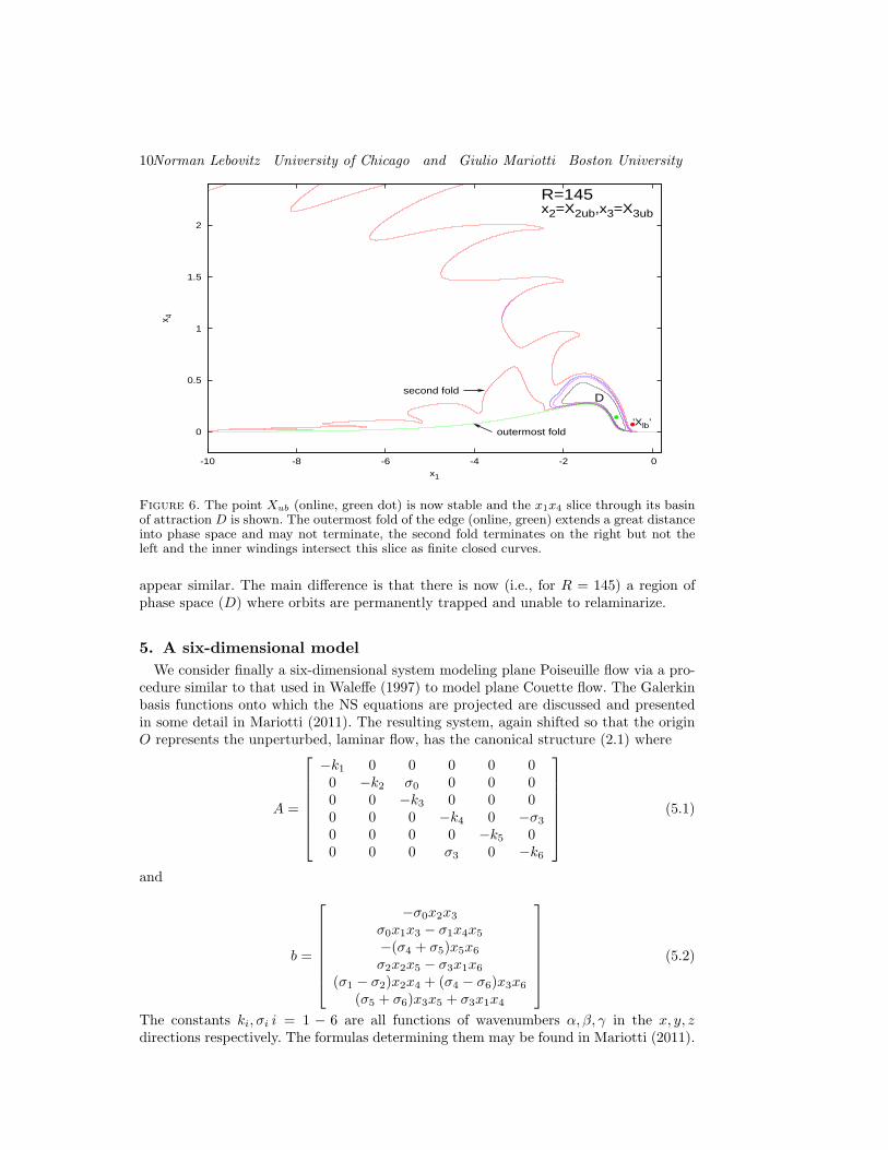
4.2.2. R = 145

For values of R > RP2the point Xub is stable. We consider its basin of attraction

D and its boundary ∂D. In this case ∂B is the union of two sets: a weak boundarycomponent (SM(Xlb), the edge) and a strong boundary component (∂D), shown inFigure 6. Consider ∂D first.

The Hopf bifurcation at R ≈ 139.7 results in a periodic orbit P for larger values of R.For the current value – R = 145 – P is found to have period T = 140.69 and Floquetexponents with magnitudes

|λ| = 1.000, 1.2003, 0.5359 × 10−3(multiplicity 2).

Thus it is unstable with a three-dimensional stable manifold, SM(P ); nearby orbits onits stable manifold are drawn toward it very rapidly. We find numerically that P lies on∂D and indeed that orbits originating on ∂D are all attracted toward P , and we concludefrom this that ∂D = SM(P ).

We now consider the edge, the weak component of ∂B. It is SM(Xlb) and we seek aslice through it by the hyperplane x2 = Xub2, x3 = Xub3.

This is also shown in Figure 6. The first, or outermost, fold of the edge (green online)appears to cover the x1 axis: we surmise that, as in the case R = 135, this would not beso along the x3 axis. The second fold (red online) is highly convoluted and appears tocover the negative, but not the positive, x1-axis. Subsequent folds are finite closed curvesthat conform their shape to that of the indicated slice of D = B(Xub).

The general similarity of these folds to those of the preceding case (R = 135) are clear,and the general features of the edge allowing all orbits to relaminarize would likewise

10Norman Lebovitz University of Chicago and Giulio Mariotti Boston University

0

0.5

1

1.5

2

-10 -8 -6 -4 -2 0

x 4

x1

R=145x2=X2ub,x3=X3ub

outermost fold

Dsecond fold

’Xlb’

Figure 6. The point Xub (online, green dot) is now stable and the x1x4 slice through its basinof attraction D is shown. The outermost fold of the edge (online, green) extends a great distanceinto phase space and may not terminate, the second fold terminates on the right but not theleft and the inner windings intersect this slice as finite closed curves.

appear similar. The main difference is that there is now (i.e., for R = 145) a region ofphase space (D) where orbits are permanently trapped and unable to relaminarize.

5. A six-dimensional model

We consider finally a six-dimensional system modeling plane Poiseuille flow via a pro-cedure similar to that used in Waleffe (1997) to model plane Couette flow. The Galerkinbasis functions onto which the NS equations are projected are discussed and presentedin some detail in Mariotti (2011). The resulting system, again shifted so that the originO represents the unperturbed, laminar flow, has the canonical structure (2.1) where

A =

−k1 0 0 0 0 00 −k2 σ0 0 0 00 0 −k3 0 0 00 0 0 −k4 0 −σ3

0 0 0 0 −k5 00 0 0 σ3 0 −k6

(5.1)

and

b =

−σ0x2x3

σ0x1x3 − σ1x4x5

−(σ4 + σ5)x5x6

σ2x2x5 − σ3x1x6

(σ1 − σ2)x2x4 + (σ4 − σ6)x3x6

(σ5 + σ6)x3x5 + σ3x1x4

(5.2)

The constants ki, σi i = 1 − 6 are all functions of wavenumbers α, β, γ in the x, y, zdirections respectively. The formulas determining them may be found in Mariotti (2011).


Here we note only that ki is positive for each i = 1 − 6, confirming the (expected)stability of the laminar solution. For the purposes of the numerical calculations of thepresent section, the values of the wavenumbers are taken to be

α = 1.1, β = π/2, γ = 5/3.

The system (2.1) with the choices of A, b(x) indicated above is easily found to possessthe group (of order four) of symmetries generated by

S1 = diag(1, 1, 1,−1,−1,−1) and S2 = diag(1,−1,−1, 1,−1, 1).

The hyperplane x4 = x5 = x6 = 0 is invariant and lies in the basin of attraction of theorigin.

5.1. Periodic Orbits

A search for equilibrium points failed. It included reduction to an eighth-order polynomialin x5, a Grobner-basis reduction using Matlab, and a search for equilibria asymptoticallyfor large R. On the other hand, a search for a stable, periodic orbit, in a region of phasespace suggested by the linearly optimal direction for the system x = Ax, was successful.Having found one such orbit for a particular value of R (we used R = 500), one canfollow it as R changes using continuation software (we used MatCont: cf. Dhooge et al.

(2003)). The result is a pattern very similar to that seen in the preceding examples, withthe difference that periodic orbits (PO) play the roles previously played by equilibriumpoints. Such orbits exist for all values of R > RSN ≈ 291.7. For the symmetry S3 = S1S2

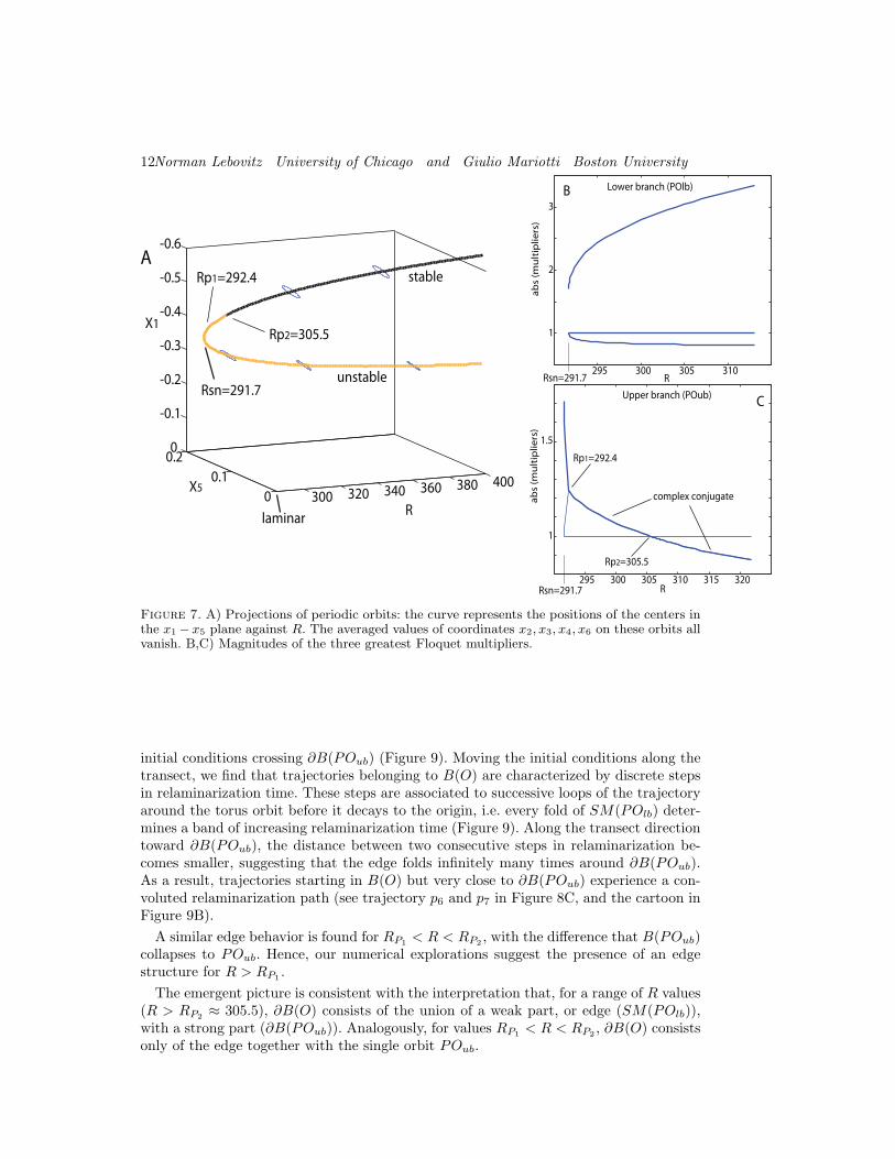
they satisfy the condition S3x(t) = x(t+T/2) where T is the period. From this one infersthat the average values of x2, x3, x4 and x6 all vanish for these orbits.

5.2. Bifurcations

The bifurcation and stability patterns of the family of periodic orbits depicted in Figure7 are analogous to those of W97.

The lower-branch periodic orbits, POlb are unstable for all values of R > RSN ≈ 291.7with a single Floquet multiplier of magnitude exceeding unity (cf. Figure 7B). ThusSM(POlb) has dimension five (codimension one).

The upper-branch orbits, on the other hand, undergo stability changes. For values ofR barely exceeding RSN the pair of Floquet multipliers of unstable type are real but,at the nearby value RP1

≈ 292.4, they coalesce and become a complex-conjugate pair,still of unstable type (cf. Figure 7C). The stability of this pair changes at a third criticalvalue RP2

≈ 305.5 and for larger values of R the upper-branch periodic orbit is stable.Thus for R > RP2

POub possesses its own basin of attraction B(POub).The bifurcation at R = RP2

is of Neimark-Sacker type and results, for R > RP2, in the

creation of an invariant torus. This torus has dimension five and forms the boundary ofthe basin of attraction of POub, and hence plays a role analogous to ∂D, the boundaryof the basin of attraction of Xub, in W97.

5.3. The structure of the edge

We first consider the case with R > RP2. As in the preceding examples, we use a continu-

ation method to identify the intersection of SM(POlb) with the hyperplane x1−x5. Alsoin this case SM(POlb) has the characteristic of an edge: initial conditions arbitrarilyclose but on different sides of SM(POlb) have qualitatively different trajectories (see forexample Fig. 8B, trajectories p4 and p5.).

We found evidence that the edge is wrapped around B(POub), as indicated by thefold shown in Figure 8. The structure of the edge is clarified by considering a transect of


300 320 340 360 380 4000

0.1

0.20

-0.1

-0.2

-0.3

-0.4

-0.5

-0.6

R

X5

X1

laminar

Rp2=305.5

Rsn=291.7

stable

unstable

295 300 305 310 315 320

1

1.5

295 300 305 310

1

2

3

Upper branch (POub)

Lower branch (POlb)

R

complex conjugate

R

ab

s (m

ult

ipli

ers

)a

bs

(mu

ltip

lie

rs)

Rp1=292.4

A

B

C

Rp1=292.4

Rp2=305.5

Rsn=291.7

Rsn=291.7

Figure 7. A) Projections of periodic orbits: the curve represents the positions of the centers inthe x1 −x5 plane against R. The averaged values of coordinates x2, x3, x4, x6 on these orbits allvanish. B,C) Magnitudes of the three greatest Floquet multipliers.

initial conditions crossing ∂B(POub) (Figure 9). Moving the initial conditions along thetransect, we find that trajectories belonging to B(O) are characterized by discrete stepsin relaminarization time. These steps are associated to successive loops of the trajectoryaround the torus orbit before it decays to the origin, i.e. every fold of SM(POlb) deter-mines a band of increasing relaminarization time (Figure 9). Along the transect directiontoward ∂B(POub), the distance between two consecutive steps in relaminarization be-comes smaller, suggesting that the edge folds infinitely many times around ∂B(POub).As a result, trajectories starting in B(O) but very close to ∂B(POub) experience a con-voluted relaminarization path (see trajectory p6 and p7 in Figure 8C, and the cartoon inFigure 9B).

A similar edge behavior is found for RP1< R < RP2

, with the difference that B(POub)collapses to POub. Hence, our numerical explorations suggest the presence of an edgestructure for R > RP1

.

The emergent picture is consistent with the interpretation that, for a range of R values(R > RP2

≈ 305.5), ∂B(O) consists of the union of a weak part, or edge (SM(POlb)),with a strong part (∂B(POub)). Analogously, for values RP1

< R < RP2, ∂B(O) consists

only of the edge together with the single orbit POub.


‘POlb’‘POub’

‘p3’

‘p1’

‘p2’

−0.4 −0.3 −0.2 −0.1 0

0.1

0.2

0.3

A

B

C

XA

torus orbit

R=307.0 (R>Rp2)

X5

‘p4’‘p5’

‘p6’‘p7’

‘POlb’‘POub’

‘POub’

X1

0.1

0.2

0.3

X5

0.1

0.2

0.3

X5

outermost fold

∂B(POub)

outermost fold

outermost fold

‘POlb’

∂B(POub)

∂B(POub)XB

Transect

crossing

∂B(POub)

Figure 8. Orbits for R = 307 > RP2, for which POub is stable (cf. Fig. 7). Upper- and

lower-branch periodic orbits are projected onto the x1−x5 plane. The other initial conditions arefixed at (x2, x3, x4, x6) =(-0.0511,-0.0391,0.0016,0.1260), which correspond to a point on POub.A) The trajectory p1 lies well on one side of SM(POlb) and relaminarizes quickly and directly,p2 well on the other side and relaminarizes less quickly and only after visiting a neighborhood ofPOub; p3 lies in B(POub). B) xA lies on SM(POlb). One orbit (p4) starts very near to xA on oneside of SM(POlb), is attracted toward POlb, lingers for a while and then decays. A second orbit(p5) starts very near to xA on the other side, follows essentially the same (yellow) path towardPOlb, lingers a while, but then has a different kind of decay (black): it first visits a neighborhoodof POub. C) xB lies on SM(POlb), but on an inner fold and close to the torus ∂B(POub). As aresult, two orbits starting close to xB , p6 and p7, experience a long and convoluted path aroundthe torus (blue). Both trajectories then approach POlb before eventually relaminarizing. Thenp6 (the lower orbit, yellow) decays immediately whereas p7 (the upper orbit, green) first revisitsa neighborhood of the torus and only then decays.


O

POlb

unstable torus

POub

(stable)

pi

pe

p1

transect

00.11 0.117

rela

min

ari

zati

on

tim

e

steps in relaminarization time

Transect crossing ∂B(POub)

tmax

X5

ABpe

pi

pi

p1 B(POub)B(O)

outermost

fold

second

fold

third

fold

Figure 9. A) Analysis of a transect of initial conditions crossing ∂B(POub), for R = 307 > RP2

(cf. Fig. 8C). The transect is aligned along the direction X5, keeping all the other initial con-ditions fixed. The first point, pi, corresponds to a trajectory that relaminarizes ‘directly’, whilethe last point, pe, corresponds to a trajectory that converges to POub. The step-wise increase inrelaminarziation time is associated to crossing folds on the edge. B) Cartoon of the phase space,with the laminar fixed point, POub, POlb, the torus orbits and a trajectory as an example,explaining the steps in relaminarization time associated to crossing folds on the edge.

6. Discussion

The most general conclusion that we draw from the preceding calculations is thatone can understand ubiquitous relaminarization in terms of the relations of invariantmanifolds in finite-dimensional systems of the form (2.1), as described in detail below(§6.1). Our picture of the edge appears to be a consistent one, occurring in severalmodels of successively higher dimension. However consistency is not the same as truth,and there is a lot more to be discovered in this subject. For example, in pipe flow there aremultiple lower-branch states (Duguet et al. (2008)), apparently all lying on a single edge,and there are also multiple upper-branch states. Moreover, the models considered heredescribe temporal behavior, whereas the full problem includes spatio-temporal behaviors.Even if the picture presented here continues to provide a building block for ubiquitousrelaminarization, a more complete description of the edge and its relations to upper-branch states awaits further study.

In both the four-dimensional model of §4 and the six-dimensional model of §5 thereis an interval of Reynolds number for which the boundary of the basin of attraction ofthe laminar state (∂B(O)) consists solely of the edge. For larger values of R the upper-branch state (Xub or POub) becomes stable and ∂B(O) is the union of the edge with thebasin boundary of the newly stable state. It is tempting to see a parallel here with theReynolds-number behavior of actual shear flows (Avila et al. (2011), Mullin (2011)): fora range of R the turbulence is transient, but beyond a critical value there is (or may be!)a turbulent attractor. On the other hand this parallel may be a spurious artifact of theextreme truncation. An understanding of how transient turbulence becomes persistentturbulence is a subject of current research. Some of this concentrates on the nature ofupper-branch states (Clever & Busse (1992, 1997); Kreilos & Eckhardt (2012)) as doesthe present paper. In particular the work of Kreilos & Eckhardt (2012) features not one


or a small number of periodic orbits but a period-doubling cascade followed by the onsetof chaos.

We briefly recapitulate the nature of the edge structure, and summarise the techniquefor producing the diagrams of this paper.

6.1. The edge

The picture of the edge obtained from the models we have considered is a codimension-one invariant manifold unbounded in some directions in phase space but – importantly– bounded in other directions at least from one side. It is the latter circumstance thatenables a pair of orbits originating on opposite sides of this manifold both to tend towardthe stable, laminar point as t → ∞. In the cases considered here the edge is a very regularobject which coincides with the stable manifold of either an equilibrium point Xlb or aperiodic orbit POlb: the ‘edge state’. In Skufca et al. (2006), for R less than a criticalvalue Rc their edge state was a periodic orbit, and the edge was likewise quite regular. ForR > Rc the edge state was a chaotic saddle. However the edge itself remained regular. Wetherefore have some reason for hoping that our characterization of the edge will continueto have meaning in some of these “wilder” cases.

This manifold cannot ‘end in thin air’ and the claim that it is finite in some directionsin phase space requires explanation. This explanation is found, in the present paper, in itsrelation to a second state, the upper-branch equilibrium point Xub (or the upper-branchperiodic orbit POub). It is found that the edge winds around the latter state infinitelyoften, never quite touching. Since the stable manifold of the edge state is of codimensionone, orbits starting near the edge but on opposite sides of it tend to be entrained byits one-dimensional unstable manifold. When the edge state is an equilibrium point, theunstable manifold consists of a pair of arcs, each of which tends to the laminar pointas t → ∞. The entrained orbits tend to the origin, although they follow quite differentevolutions depending on the side of the edge from which they originated. A similar pictureis found when the edge state is a periodic orbit, except that now the unstable manifoldis two-dimensional.

The nature of an orbit and the time for its relaminarization depend on whether thestarting point of the orbit lies above the edge – in which case it must circumnavigatethe upper-branch state and its associated invariant manifolds – or below the edge –in which case it has a more direct route to relaminarization. However, there are twofurther contingencies that may contribute to the relaminarization time of an orbit. Oneis proximity to the edge: the closer it is to the edge the longer it will linger near the edgestate before relaminarizing. The second is related to the fold structure of the edge nearthe upper-branch state: an orbit that starts between two inner folds is trapped withinthe fold structure until it winds its way out.

6.2. Technique

The computational technique for finding slices of the boundary of the basin of attractionof the lower-branch states found in §4 of this paper is straightforward. We start with apoint known to lie on that boundary. For example, in Figure 4, the point Xlb is such apoint. Alternatively, we may start with a pair of points of which one relaminarizes quickly(an ‘inside’ point) and one slowly (an ‘outside’ point) and produce, by bisection, such apair that lie extremely close to one another, and which therefore straddle the edge. Weslightly alter one of their coordinates (x1 say) and repeat this procedure so as to find anew pair of points straddling the edge. Once a point in Rn lying on the edge has beenlocated, we can move around in any direction in Rn seeking more edge points in this way.

An alternative method is to locate and record edge points via the transect method


described in §5. A lifetime landscape map, e.g. Skufca et al. (2006), is first constructedto isolate the general locations of the edge folds. Then, refined transects across the foldsare used to identify discrete steps in relaminarization time (e.g., Fig. 9A), which areassociated to increasing loops of the trajectory around the upper-branch state.

Parts of this work were done during the summer of 2011 at the Geophysical Fluid Dy-namics program at the Woods Hole Oceanographic Institution. We are grateful for thesupport of the program and the contributions to it of the National Science Foundationand the Office of Naval Research through grants OCE-0824636 and N00014-09-1-0844 re-spectively. We would also like to acknowledge helpful discussions with Matthew Chantry,Bruno Eckhardt, Tobias Schneider and Fabian Waleffe.

REFERENCES

Avila, D., Moxey, D., de Lozar, A., Avila, M., Barkley, D. & Hof, B. 2011 The onsetof turbulence in pipe flow. Science 333, 192–196.

Butler, K.M. & Farrell, B.F. 1992 Three-dimensional optimal disturbances in viscous flows.Phys. Fluids A 12, 1637–1650.

Clever, R.M. & Busse, F.H. 1992 Three-dimensional convection in a horizontal fluid layersubjected to constant shear. JFM 234, 511–527.

Clever, R.M. & Busse, F.H. 1997 Tertiary and quaternary solutions for plane couette flow.JFM 344, 137–153.

Cossu, C. 2005 An optimality condition on the minimum energy threshold in subcritical insta-bilities. C. R. Mecanique 333, 331–336.

Dauchot, O. & Vioujard, N. 2000 Phase space analysis of a dynamical model for the sub-critical transition to turbulence in plane couette flow. Eur. Phys. J. B 14, 377–381.

Dhooge, A., Govaerts, W. & Kuznetsov, Yu. A. 2003 matcont: A matlab package fornumerical bifurcation analysis of odes. ACM TOMS 29, 141–164.

Duguet, Y., Willis, A.P. & Kerswell, R. 2008 Transition in pipe flow: the saddle structureon the boundary of turbulence. JFM 613, 255–274.

Eckhardt, B. 2008 Turbulence transition in pipe flow: some open questions. Nonlinearity 21,T1–T11.

Kreilos, T. & Eckhardt, B. 2012 Periodic orbits near the onset of chaos in plane couetteflow. http://arxiv.org/abs/1205.0347 .

Lebovitz, N. 2009 Shear-flow transition: the basin boundary. Nonlinearity 22, 2645–2655.Lebovitz, N. 2012 Boundary collapse in models of shear-flow transition. CNSNS 17, 2095–2100.Mariotti, G. 2011 A low dimensional model for shear turbulence in plane poiseuille flow:

an example to understand the edge. In Proceedings of the Program in Geophysical FluidDynamics. Woods Hole Oceanographic Institution.

Mullin, T. 2011 Experimental studies of transition to turbulence in a pipe. Ann. Rev. Fl. Mech43, 1–24.

Skufca, J.D., Yorke, J.A. & Eckhardt, B. 2006 Edge of chaos in a parallel shear flow.Phys. Rev. Lett. 96, 174101.

Vollmer, J., Schneider, T.M. & Eckhardt, B. 2009 Basin boundary, edge of chaos andedge state in a two-dimensional model. New J. Phys. 11, 013040.

Waleffe, F. 1997 On a self-sustaining process in shear flows. Phys. Fluids 9 (4), 883–900.

edges in models of shear flow - university of...

Documents