edge spinning algorithm for implicit...

thentedplicated

issented

es andlization.n

bjectn

phere.

Applied Numerical Mathematics 49 (2004) 331–342www.elsevier.com/locate/apnum

Edge spinning algorithm for implicit surfaces✩

M. Cermak, V. Skala∗

Department of Computer Science, University of West Bohemia, Univerzitni 8, Box 314, 306 14 Plzen, Czech Republic

Abstract

This paper presents a new fast method for polygonization of implicit surfaces. Our method put emphasis onshape of triangles generated and on the polygonization speed. The main advantages of the triangulation preseare simplicity and the stable features that can be used for future expansion. The implementation is not comand only the standard data structures are used. This algorithm is based on the surface tracking scheme and itcompared with the well-known marching cubes algorithm that is based on the similar principle. The prealgorithm is accelerated by the space subdivision which is an effective technique to speed-up any geometric of thistype. 2004 IMACS. Published by Elsevier B.V. All rights reserved.

Keywords: Polygonization; Triangulation; Implicit surfaces; Marching method; Edge spinning; Acceleration

1. Introduction

Implicit surfaces seem to be one of the most appealing concepts for building complex shapsurfaces. They have become widely used in several applications in computer graphics and visua

An implicit surface is mathematically defined as a set of points in spacex that satisfy the equatiof (x) = 0. Thus, visualizing implicit surfaces typically consists in finding the zero-set off , which maybe performed either by polygonizing the surface or by direct ray-tracing.

There are two different definitions for implicit surfaces. The first one [2,3] defines an implicit oasf (x) < 0 (function f1(x) below) and the second,F -rep [7,12], (functional representation, functiof2(x)) defines it asf (x) � 0. In our implementation, we use theF -rep definition of implicit objects. Theimplicit functions described below show the differences between both definitions for the function s

f1(x): x2 + y2 + z2 − r2 = 0, f2(x): r2 − x2 − z2 = 0.

✩ This work was supported by the Ministry of Education of the Czech Republic – project MSM 235200005.* Corresponding author.

E-mail addresses: [email protected] (M. Cermak), [email protected] (V. Skala).

0168-9274/$30.00 2004 IMACS. Published by Elsevier B.V. All rights reserved.doi:10.1016/j.apnum.2003.12.011

332 M. Cermak, V. Skala / Applied Numerical Mathematics 49 (2004) 331–342

Iso-surface extraction is needed for the visualization purposes that have a set of triangles as a result.Existing techniques may be classified into three categories.

ling theells are

ulation

implicit

he maintandardorhood

ex into

e; left

Spatial sampling techniques regularly or adaptively sample the space to find the cells straddimplicit surface, and tessellate those cells to create overall polygonization [2,3,9]. In general, ceither cubes or tetrahedra.

Surface tracking approaches (also known as continuation method) iteratively create a triangfrom a seed element by marching along the surface [1,2,5,6,14].

Surface fitting techniques progressively adapt and deform an initial mesh to converge to thesurface.

2. Data structures

The presented algorithm uses only the standard data structures used in computer graphics. Tdata structure is the edge that is used as a basic building block for polygonization. We use the swinding edge and therefore, the resulting polygonal mesh is correct and complete with neighbamong all triangles generated. The basic data structures used there are:

• edge—winding edge;• active edge—an edge that lies on the triangulated area’s border; implemented as an ind

winding edge’s array;• list of active edges—dynamically allocated list of active edges;• point—if a point lies on an active edge it contains also two pointers to left and right active edg

and right directions are in active edges orientation.

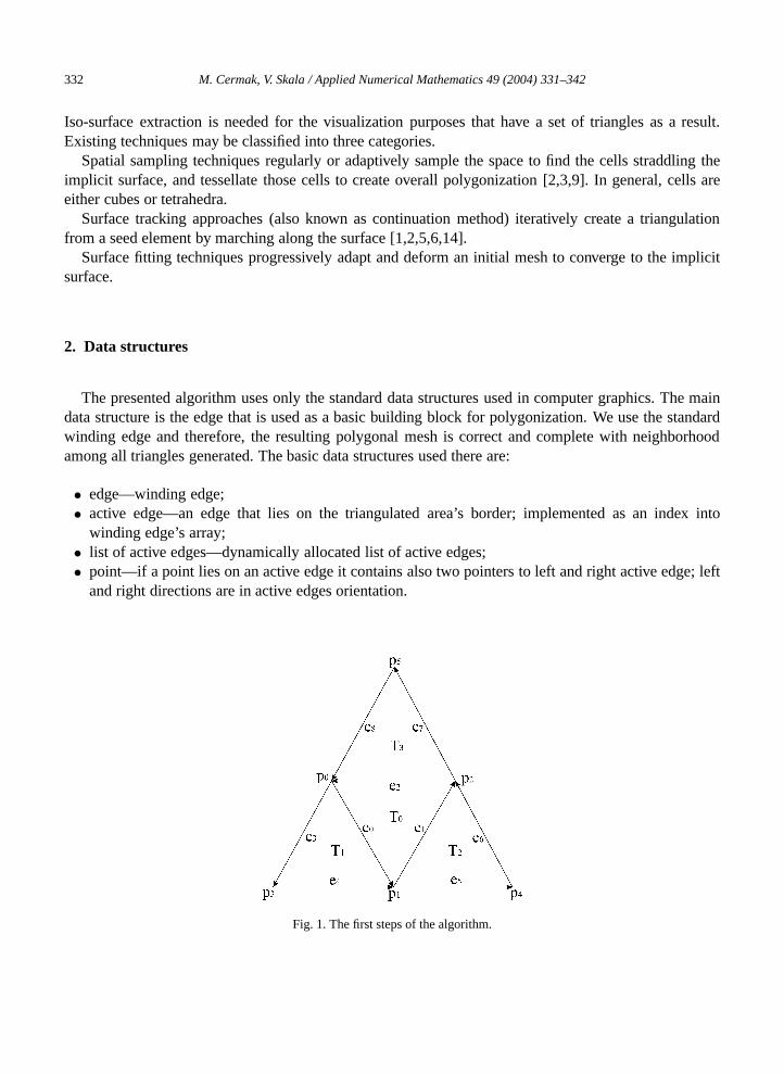
Fig. 1. The first steps of the algorithm.

M. Cermak, V. Skala / Applied Numerical Mathematics 49 (2004) 331–342 333

3. Principle of our algorithm

itations.for thiswhole

dges

e

can berching in

ought

Our algorithm is based on the surface tracking scheme and therefore, there are several limA starting point must be determined and only one separated implicit surface can by polygonizedfirst point. Several disjoint surfaces can be polygonized from a starting point for each of them. Thealgorithm consists of following steps:

(1) Find a starting pointp0.(2) Create a first triangleT0, see Fig. 1.(3) Include the edges(e0, e1, e2) of the first triangleT0 into the active edges list.(4) Polygonize the first active edgee from the active edges list.(5) Delete the actual active edgee from the active edges list and include the new generated active e

at the end of the active edges list.(6) Check the distance between the new generated pointpnew and all the other points which lie on th

border of already triangulated area (which lie in all the other active edges).(7) If the active edges list is not empty return to step 4.

4. Starting point

There are several methods for finding a starting point on an implicit surface. These algorithmsbased on some random search method as in [2] or on more sophisticated approach. In [14], seaconstant direction from an interior of an implicit object is used.

In our approach, we use a simple algorithm for finding a starting point. A starting point is sfrom any place in a defined area in the direction of a gradient vector∇f of an implicit functionf . Thealgorithm looks for a pointp0 that satisfies the equationf (p0) = 0.

5. First triangle

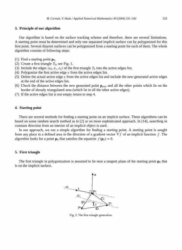
The first triangle in polygonization is assumed to lie near a tangent plane of the starting pointp0 thatis on the implicit surface.

Fig. 2. The first triangle generation.


(1) Determine the normal vectorn = (nx, ny, nz) in the starting pointp0, see Fig. 2,

ribed

n forare

tion of adirectiont ofdefined

riangle

.

r

leso

n = ∇f/‖∇f‖.(2) Determine the tangent vectort as in [5]. If (nx > 0.5) or (ny > 0.5) then t = (ny,−nx,0); else

t = (−nz,0, nx).(3) Use the tangent vectort as a fictive active edge and use the edge spinning algorithm (desc

bellow) for computation coordinates of the second pointp1. The pair of points(p0,p1) forms thefirst edgee0.

(4) Polygonize the first edgee0 with the edge spinning algorithm for getting the third pointp2. Points(p0,p1,p2) and edges(e0, e1, e2) form the first triangleT0.

6. Edge spinning algorithm

The main goal of this work is a numerical stability of a surface point coordinates’ computatioobjects which are defined by the implicit function. Differential properties for each implicit functiondifferent in dependence on the modeling techniques [6,7,10,12,13] and the accurate determinaposition of a surface vertex depends on them. In general, a surface vertex position is searched inof a gradient vector of an implicit functionf , e.g., in [5]. In many cases, the computing of a gradienthe functionf is influenced by a major error. Because of these reasons, in our approach, we havethese restrictions for finding a new surface pointpnew.

• The new pointpnew is sought in a constant distance, i.e., on a circle; then each new generated tpreserves the desired accuracy of polygonization—the average edge’s lengthδe. The circle radius isproportional to theδe.

• The circle lies in the plane that is defined by the normal vector of triangleTold (see Fig. 3) and axisoof the actual edgee; this guarantees that the new generated triangle is well shaped (isosceles)

Then, the algorithm is:

(1) Set the pointpnew to its initial position; the initial position is on the triangle’sTold plane on the otheside of the edgee, see Fig. 3. Let the angle of the initial position beα = 0.

(2) Compute the function valuesf (pnew) = f (α), f (p′new) = f (α +�α)—initial position rotated by the

angle+�α, f (p′′new) = f (α − �α)—initial position rotated by the angle−�α; the rotation axis is

the edgee.(3) Determine the right direction of rotation; if|f (α + �α)| < |f (α)| then+�α else−�α.(4) Let the function valuesf1 = f (α) andf2 = f (α ± �α); actualize angleα = α ± �α.(5) If (f1 ·f2) < 0 then compute the accurate coordinates of the new pointpnew by the binary subdivision

between the last two points which correspond to function valuesf1 andf2; else return to step 4.(6) Check if both trianglesTold andTnew do not cross each other; if the angle between these triangβ

is greater thanβlim (see Fig. 4) then pointpnew is accepted; else pointpnew is rejected and return tstep 4.


cent

Fig. 3. The edge spinning algorithm principle.

Fig. 4. The angle between two triangles; the view is in direction of edge’s vectore.

7. Active edge polygonization

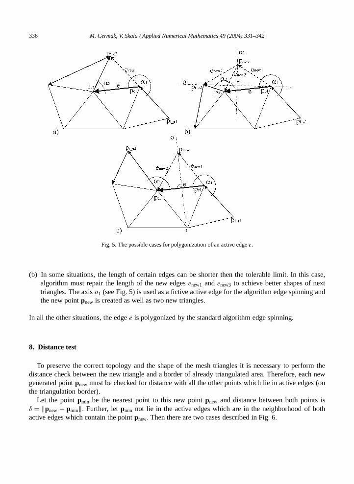
Polygonization of an active edgee consists of several steps. At first, the algorithm checks adjaactive edges of the active edgee and determines which case appeared, see Fig. 5.

• If (αi < αlim_1) then case (a);i = 1,2.• If (α2 < αlim _2) and(‖pe1 − pr_e2‖ < δlim _1) then case (a); analogically forα1.• If (α2 > αlim _3) and(‖pe1 − pr_e2‖ < δlim _2) then case (b); analogically forα1.• else case (c).

The relations among limit angles areαlim _1 < αlim _2 � αlim_3.Possible cases which are illustrated in Fig. 5 are:

(a) In this case, algorithm creates a new triangle and includes a new active edgeenew to the end of theactive edges list.


is case,xtg and

form theach news (on

isoth

Fig. 5. The possible cases for polygonization of an active edgee.

(b) In some situations, the length of certain edges can be shorter then the tolerable limit. In thalgorithm must repair the length of the new edgesenew1 andenew3 to achieve better shapes of netriangles. The axiso1 (see Fig. 5) is used as a fictive active edge for the algorithm edge spinninthe new pointpnew is created as well as two new triangles.

In all the other situations, the edgee is polygonized by the standard algorithm edge spinning.

8. Distance test

To preserve the correct topology and the shape of the mesh triangles it is necessary to perdistance check between the new triangle and a border of already triangulated area. Therefore, egenerated pointpnew must be checked for distance with all the other points which lie in active edgethe triangulation border).

Let the pointpmin be the nearest point to this new pointpnew and distance between both pointsδ = ‖pnew − pmin‖. Further, letpmin not lie in the active edges which are in the neighborhood of bactive edges which contain the pointpnew. Then there are two cases described in Fig. 6.


ngles

lutionactive

en angles

the list

tiventcached

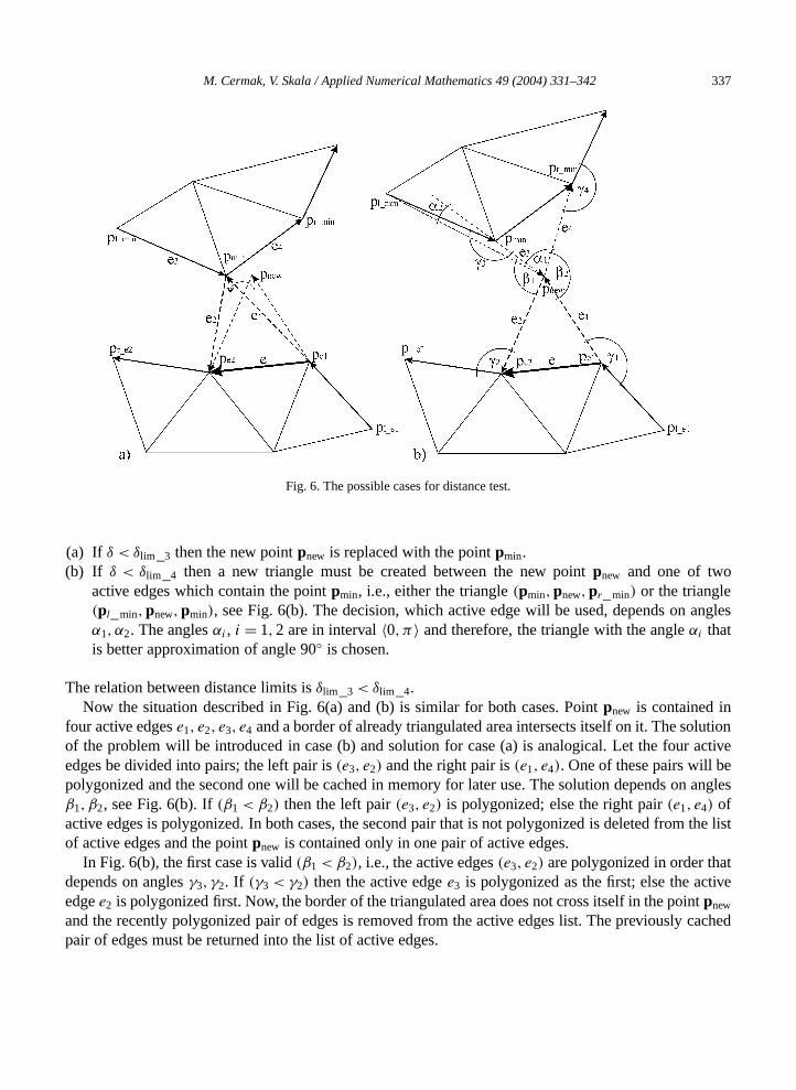
Fig. 6. The possible cases for distance test.

(a) If δ < δlim _3 then the new pointpnew is replaced with the pointpmin.(b) If δ < δlim _4 then a new triangle must be created between the new pointpnew and one of two

active edges which contain the pointpmin, i.e., either the triangle(pmin,pnew,pr_min) or the triangle(pl_min,pnew,pmin), see Fig. 6(b). The decision, which active edge will be used, depends on aα1, α2. The anglesαi , i = 1,2 are in interval〈0, π〉 and therefore, the triangle with the angleαi thatis better approximation of angle 90◦ is chosen.

The relation between distance limits isδlim _3 < δlim _4.Now the situation described in Fig. 6(a) and (b) is similar for both cases. Pointpnew is contained in

four active edgese1, e2, e3, e4 and a border of already triangulated area intersects itself on it. The soof the problem will be introduced in case (b) and solution for case (a) is analogical. Let the fouredges be divided into pairs; the left pair is(e3, e2) and the right pair is(e1, e4). One of these pairs will bpolygonized and the second one will be cached in memory for later use. The solution depends oβ1, β2, see Fig. 6(b). If(β1 < β2) then the left pair(e3, e2) is polygonized; else the right pair(e1, e4) ofactive edges is polygonized. In both cases, the second pair that is not polygonized is deleted fromof active edges and the pointpnew is contained only in one pair of active edges.

In Fig. 6(b), the first case is valid(β1 < β2), i.e., the active edges(e3, e2) are polygonized in order thadepends on anglesγ3, γ2. If (γ3 < γ2) then the active edgee3 is polygonized as the first; else the actedgee2 is polygonized first. Now, the border of the triangulated area does not cross itself in the poipnew

and the recently polygonized pair of edges is removed from the active edges list. The previouslypair of edges must be returned into the list of active edges.


9. Space subdivision principle

rowing

to anyahead.en the

orhood.

b-s in

in;int lies

rithm

tation.

The original distance check algorithm takes more time if a required scene detail grows (gnumber of points on the triangulation border). The algorithm complexity for one included point is O(N),whereN is a number of points in active edges. In aspect that the new included point can lie nearpoint of the boundary, it is not possible to determine some subset of candidates to nearest point

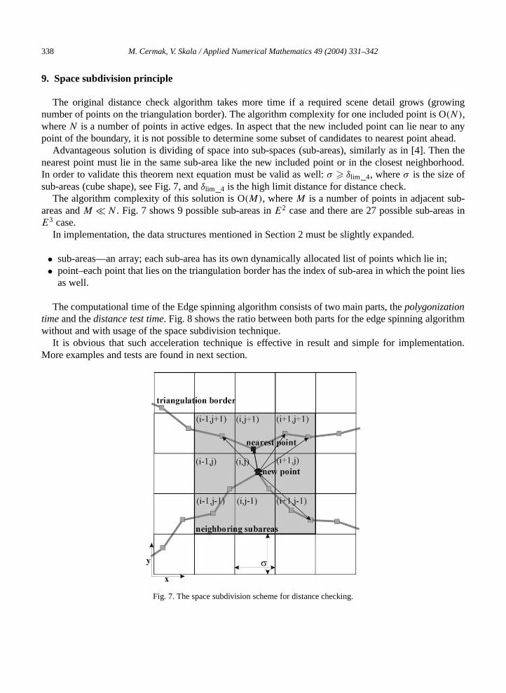
Advantageous solution is dividing of space into sub-spaces (sub-areas), similarly as in [4]. Thnearest point must lie in the same sub-area like the new included point or in the closest neighbIn order to validate this theorem next equation must be valid as well:σ � δlim _4, whereσ is the size ofsub-areas (cube shape), see Fig. 7, andδlim _4 is the high limit distance for distance check.

The algorithm complexity of this solution is O(M), whereM is a number of points in adjacent suareas andM � N . Fig. 7 shows 9 possible sub-areas inE2 case and there are 27 possible sub-areaE3 case.

In implementation, the data structures mentioned in Section 2 must be slightly expanded.

• sub-areas—an array; each sub-area has its own dynamically allocated list of points which lie• point–each point that lies on the triangulation border has the index of sub-area in which the po

as well.

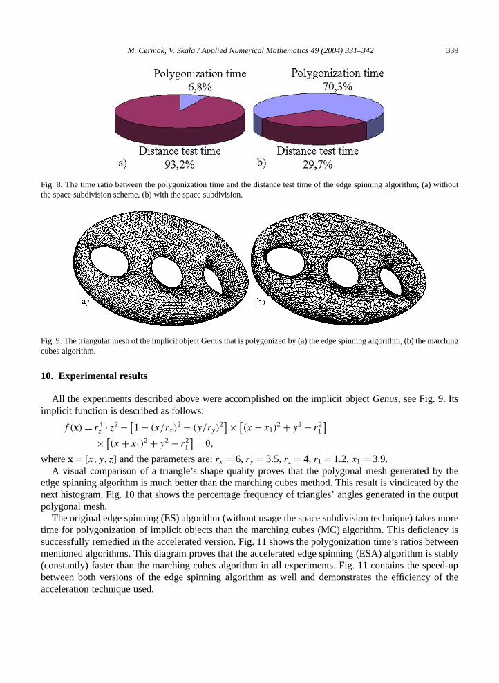
The computational time of the Edge spinning algorithm consists of two main parts, thepolygonizationtime and thedistance test time. Fig. 8 shows the ratio between both parts for the edge spinning algowithout and with usage of the space subdivision technique.

It is obvious that such acceleration technique is effective in result and simple for implemenMore examples and tests are found in next section.

Fig. 7. The space subdivision scheme for distance checking.


without

arching

by thed by thee output

s morecy isetweens stablyeed-up

y of the

Fig. 8. The time ratio between the polygonization time and the distance test time of the edge spinning algorithm; (a)the space subdivision scheme, (b) with the space subdivision.

Fig. 9. The triangular mesh of the implicit object Genus that is polygonized by (a) the edge spinning algorithm, (b) the mcubes algorithm.

10. Experimental results

All the experiments described above were accomplished on the implicit objectGenus, see Fig. 9. Itsimplicit function is described as follows:

f (x) = r4z · z2 − [

1− (x/rx)2 − (y/ry)

2] × [

(x − x1)2 + y2 − r2

1

]

× [(x + x1)

2 + y2 − r21

] = 0,

wherex = [x, y, z] and the parameters are:rx = 6, ry = 3.5, rz = 4, r1 = 1.2, x1 = 3.9.A visual comparison of a triangle’s shape quality proves that the polygonal mesh generated

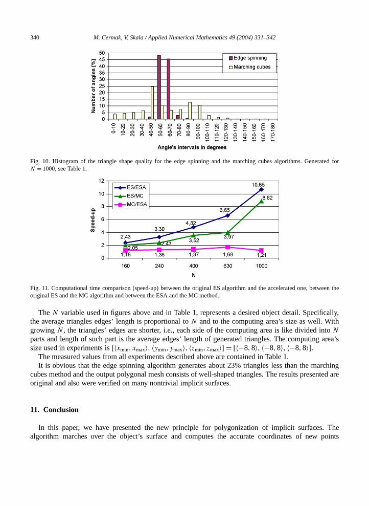
edge spinning algorithm is much better than the marching cubes method. This result is vindicatenext histogram, Fig. 10 that shows the percentage frequency of triangles’ angles generated in thpolygonal mesh.

The original edge spinning (ES) algorithm (without usage the space subdivision technique) taketime for polygonization of implicit objects than the marching cubes (MC) algorithm. This deficiensuccessfully remedied in the accelerated version. Fig. 11 shows the polygonization time’s ratios bmentioned algorithms. This diagram proves that the accelerated edge spinning (ESA) algorithm i(constantly) faster than the marching cubes algorithm in all experiments. Fig. 11 contains the spbetween both versions of the edge spinning algorithm as well and demonstrates the efficiencacceleration technique used.


rated for

the

ifically,ithintog area’s

archingented are

. Thepoints

Fig. 10. Histogram of the triangle shape quality for the edge spinning and the marching cubes algorithms. GeneN = 1000, see Table 1.

Fig. 11. Computational time comparison (speed-up) between the original ES algorithm and the accelerated one, betweenoriginal ES and the MC algorithm and between the ESA and the MC method.

TheN variable used in figures above and in Table 1, represents a desired object detail. Specthe average triangles edges’ length is proportional toN and to the computing area’s size as well. Wgrowing N , the triangles’ edges are shorter, i.e., each side of the computing area is like dividedN

parts and length of such part is the average edges’ length of generated triangles. The computinsize used in experiments is[〈xmin, xmax〉, 〈ymin, ymax〉, 〈zmin, zmax〉] = [〈−8,8〉, 〈−8,8〉, 〈−8,8〉].

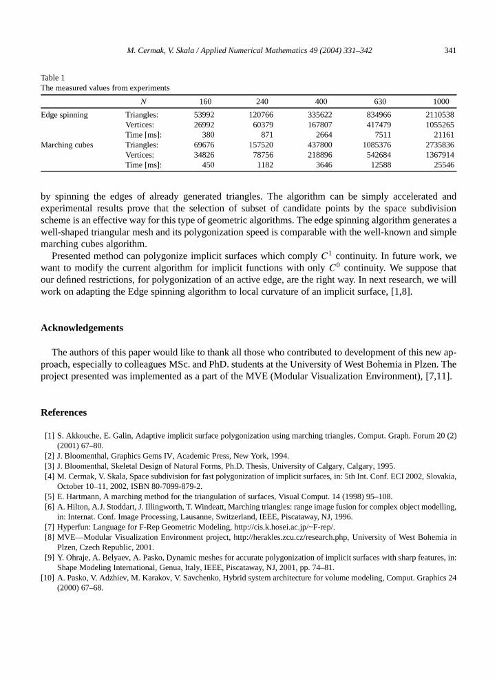
The measured values from all experiments described above are contained in Table 1.It is obvious that the edge spinning algorithm generates about 23% triangles less than the m

cubes method and the output polygonal mesh consists of well-shaped triangles. The results presoriginal and also were verified on many nontrivial implicit surfaces.

11. Conclusion

In this paper, we have presented the new principle for polygonization of implicit surfacesalgorithm marches over the object’s surface and computes the accurate coordinates of new


Table 1The measured values from experiments

538651836146

ted anddivision

erates asimple

twe will

ew ap-en. The,11].

20 (2)

vakia,

,

res, in:

hics 24

N 160 240 400 630 1000

Edge spinning Triangles: 53992 120766 335622 834966 2110Vertices: 26992 60379 167807 417479 10552Time [ms]: 380 871 2664 7511 2116

Marching cubes Triangles: 69676 157520 437800 1085376 2735Vertices: 34826 78756 218896 542684 13679Time [ms]: 450 1182 3646 12588 2554

by spinning the edges of already generated triangles. The algorithm can be simply acceleraexperimental results prove that the selection of subset of candidate points by the space subscheme is an effective way for this type of geometric algorithms. The edge spinning algorithm genwell-shaped triangular mesh and its polygonization speed is comparable with the well-known andmarching cubes algorithm.

Presented method can polygonize implicit surfaces which complyC1 continuity. In future work, wewant to modify the current algorithm for implicit functions with onlyC0 continuity. We suppose thaour defined restrictions, for polygonization of an active edge, are the right way. In next research,work on adapting the Edge spinning algorithm to local curvature of an implicit surface, [1,8].

Acknowledgements

The authors of this paper would like to thank all those who contributed to development of this nproach, especially to colleagues MSc. and PhD. students at the University of West Bohemia in Plzproject presented was implemented as a part of the MVE (Modular Visualization Environment), [7

References

[1] S. Akkouche, E. Galin, Adaptive implicit surface polygonization using marching triangles, Comput. Graph. Forum(2001) 67–80.

[2] J. Bloomenthal, Graphics Gems IV, Academic Press, New York, 1994.[3] J. Bloomenthal, Skeletal Design of Natural Forms, Ph.D. Thesis, University of Calgary, Calgary, 1995.[4] M. Cermak, V. Skala, Space subdivision for fast polygonization of implicit surfaces, in: 5th Int. Conf. ECI 2002, Slo

October 10–11, 2002, ISBN 80-7099-879-2.[5] E. Hartmann, A marching method for the triangulation of surfaces, Visual Comput. 14 (1998) 95–108.[6] A. Hilton, A.J. Stoddart, J. Illingworth, T. Windeatt, Marching triangles: range image fusion for complex object modelling

in: Internat. Conf. Image Processing, Lausanne, Switzerland, IEEE, Piscataway, NJ, 1996.[7] Hyperfun: Language for F-Rep Geometric Modeling, http://cis.k.hosei.ac.jp/~F-rep/.[8] MVE—Modular Visualization Environment project, http://herakles.zcu.cz/research.php, University of West Bohemia in

Plzen, Czech Republic, 2001.[9] Y. Ohraje, A. Belyaev, A. Pasko, Dynamic meshes for accurate polygonization of implicit surfaces with sharp featu

Shape Modeling International, Genua, Italy, IEEE, Piscataway, NJ, 2001, pp. 74–81.[10] A. Pasko, V. Adzhiev, M. Karakov, V. Savchenko, Hybrid system architecture for volume modeling, Comput. Grap

(2000) 67–68.


[11] M. Rousal, V. Skala, Modular visualization environment—MVE, in: Int. Conf. ECI 2000, Herlany, Slovakia, 2000,pp. 245–250, ISBN 80-88922-25-9.

deling

sity of

[12] A.M. Rvachov, Definition of R-functions, http://www.mit.edu/~maratr/rvachev/p1.htm.[13] V. Shapiro, I. Tsukanov, Implicit functions with guaranteed differential properties, ACM Symposium on Solid Mo

and Applications, Ann Arbor, Michigan, ACM Press, New York, 1999, pp. 258–269.[14] F. Triquet, F. Meseure, Ch. Chaillou, Fast polygonization of implicit surfaces, in: WSCG 2001 Int. Conf., Univer

West Bohemia in Pilsen, 2001, p. 162.

edge spinning algorithm for implicit...

Documents