eddy current flow measurements in the fftf

PNNL-26202

Eddy Current Flow Measurements in the FFTF December 2016

DL Nielsen RP Omberg DL Polzin BJ Makenas

~ Terra Power:

Prepared for the TerraPower, LLC under a Commercial Work for Others Agreement with the

U.S. Department of Energy under Contract DE-ACOS-76RL01830

U.S. DEPARTMENT OF

ENERGY

DISCLAIMER This report was prepared as an account of work sponsored by an agency of the United States Government. Neither the United States Government nor any agency thereof, nor Battelle Memorial Institute, nor any of their employees, makes any warranty, express or implied, or assumes any legal liability or responsibility for the accuracy, completeness, or usefulness of any information, apparatus, product, or process disclosed, or represents that its use would not infringe privately owned rights. Reference herein to any specific commercial product, process, or service by trade name, trademark, manufacturer, or otherwise does not necessarily constitute or imply its endorsement, recommendation, or favoring by the United States Government or any agency thereof, or Battelle Memorial Institute. The views and opinions of authors expressed herein do not necessarily state or reflect those of the United States Government or any agency thereof. PACIFIC NORTHWEST NATIONAL LABORATORY operated by BATTELLE for the UNITED STATES DEPARTMENT OF ENERGY under Contract DE-AC05-76RL01830 Printed in the United States of America Available to DOE and DOE contractors from the Office of Scientific and Technical Information,

P.O. Box 62, Oak Ridge, TN 37831-0062; ph: (865) 576-8401 fax: (865) 576-5728

email: [email protected] Available to the public from the National Technical Information Service, U.S. Department of Commerce, 5285 Port Royal Rd., Springfield, VA 22161

ph: (800) 553-6847 fax: (703) 605-6900

email: [email protected] online ordering: http://www.ntis.gov/ordering.htm

This document was printed on recycled paper.

(9/2003)

PNNL-26202

Eddy Current Flow Measurements in the FFTF DL Nielsen RP Omberg DL Polzin BJ Makenas December 2016 Prepared for the TerraPower, LLC under a Commercial Work for Others Agreement with the U.S. Department of Energy under Contract DE-AC05-76RL01830

Pacific Northwest National Laboratory Richland, Washington 99352

ii

Executive Summary

The Fast Flux Test Facility (FFTF) is the most recent liquid metal reactor (LMR) to be designed,

constructed, and operated by the U.S. Department of Energy (DOE). The 400-MWt sodium-

cooled, fast-neutron flux reactor plant was designed for irradiation testing of nuclear reactor fuels

and materials for liquid metal fast breeder reactors. Following shut down of the Clinch River

Breeder Reactor Plant (CRBRP) project in 1983, FFTF continued to play a key role in providing

a test bed for demonstrating performance of advanced fuel designs and demonstrating operation,

maintenance, and safety of advanced liquid metal reactors. The FFTF Program provides valuable

information for potential follow-on reactor projects in the areas of plant system and component

design, component fabrication, fuel design and performance, prototype testing, site construction,

and reactor control and operations. This report provides HEDL-TC-1344, “ECFM Flow

Measurements in the FFTF Using Phase-Sensitive Detectors”, March 1979.

iii

Acronyms

ARD Advanced Reactor Division

CRBRP Clinch River Breeder Reactor Plant

DOE U.S. Department of Energy

ECFM Eddy-Current Flowmeter

FFTF Fast Flux Test Facility

FTR Fast Test Reactor

LMFBR Liquid Metal Fast Breeder Reactor

LMR Liquid Metal Reactor

iv

Contents Executive Summary ...................................................................................................................................... ii 1.0 Eddy Current Flow Measurements in the FFTF ................................................................................... 1

1

1.0 Eddy Current Flow Measurements in the FFTF

The Fast Flux Test Facility (FFTF) is the most recent liquid metal reactor (LMR) to operate in

the United States, from 1982 to 1992.The 400-MWt sodium-cooled, low-pressure, high-

temperature, fast-neutron flux, nuclear fission test reactor was designed specifically to irradiate

Liquid Metal Fast Breeder Reactor (LMFBR) fuel and components in prototypical temperature

and flux conditions. FFTF played a key role in LMFBR development and testing activities. The

reactor provided extensive capability for in-core irradiation testing, including eight core positions

that could be used with independent instrumentation for the test specimens. In addition to

irradiation testing capabilities, FFTF provided long-term testing and evaluation of plant

components and systems for LMFBRs.

This report provides HEDL-TC-1344, “ECFM Flow Measurements in the FFTF Using Phase-

Sensitive Detectors”, W.T. Nutt and J.L. Stringer, Hanford Engineering Development

Laboratory, March 1979. The Eddy-Current Flowmeter (ECFM) is an accurate electromagnetic

device for measuring the velocity of a conductor along the longitudinal axis of the flowmeter.

Misconceptions about the inherent accuracy of the flow signal resulted in the belief that the

ECFM had little flow sensitivity at low flow velocities (see References 1, 2 and 3 of TC-1344).

The report dispelled that notion and describes the equipment and procedures for accurately

measuring very low flows in the FFTF using an Eddy Current Flowmeter. Calibration results

from the Transient Test Loop were analyzed and are presented in the report. Analysis of the

hardware operation in extracting a flow reading from the flowmeter signal was used to show the

efficacy of the phase-sensitive detection procedure

y Pacific Northwest

NATIONAL LABORATORY

Proudly Operated by Battelle Since 1965

902 Battelle Boulevard

P.O. Box 999

Richland, WA 99352

1-888-375-PNNL (7665)

www.pnnl.gov

U .S. DEPARTMENT OF

ENERGY

HEDL-TC-1344

ECFM Flow Measurements in the FFTF

Using Phase Sensitive Detectors

Provided with PNNL-26202

TC-1344

ECFM FLOW MEASUREMENTS IN THE FFTF USING PHASE-SENSITIVE DETECTORS

Hanford Engineering Development Laboratory

· W. T. Nutt

J. L. Stringer

March 1979

HANFORD ENGINEERING DEVELOPMENT LABORATORY Operated by Westinghouse Hanford Company

P.O. Box 1970 Richland, WA 99352 A Subsidiary of Westinghouse Electric Corporation

Prepared for the U.S. Department of Energy under Contract No. EY-76-C-14-2170 Provided with PNNL-26202

ECFM FLOW MEASUREMENTS IN THE FFTF USING PHASE-SENSITIVE DECTECORS

W. T. Nutt J. L. Stringer

ABSTRACT

IIL.UL.- I I., I J"t't

The equipment and procedures for accurately measuring very low flows in the Fast Flux Test Facility using an Eddy Current Flowrneter are described. Calibration results from the Tr~nsient Test Loop are analyzed and presented. Analysis o'f the hardware operation in extracting a flow readi_ng from the flowneter signal is used to show the efficacy of the phase-sensitive detection procedure.

iii Provided with PNNL-26202

ACKNOWLEDGEMENT

The authors would like to express their appreciation to W. L.-Thorne for his invaluable assistance and cooperation during the testing phase of this work.

iv Provided with PNNL-26202

Abstract Acknowledgement Figures Tables

l.O INTRODUCTION l.l Overview l. 2 FFTF Goa 1 s

2.0 HARDWARE DESCRIPTION 2. l ECFM

CONTENTS

2.2 Amplitude Detection Electronics 2.3 Phase-Sensitive Detection Electronics

3.0 ANALYSIS 3. r ECFM 3.2 Amplitude Detection 3.3 Phase-Sensitive Detection 3.4 Error Sources

3.4.l Hardware Biases 3.4.2 Electronics Biases 3.4.3 Noise

3.5 Calibration Results 3.5.l Calibration Curves 3.5.2 Conclusions

4.0 PLANT PROCEDURE 4.l Phase-Sensitive Detector Setup

4.1.l Fuel Assemblies 4.1.2 Reflectors

4.2 Rias Shift Checks

5. 0 PHASE-SENSITIVE ELECTRONIC CALIBRATION 5.1 Standard In-Laboratory Calibration 5.2 In-Field Calibration

6.0 REFERENCES

APPENDICES

V

l

l

l

.8

iii iv

V

vi

8

8

11

18

18

19

22

31

31 33 33

33 34 54

55 55 55

55 56

57

57

57

60


Figure

1-1

l-2a l-2b , 1-3

2-1

2-2 2-3 2-4 2-5 2-6 2-7

3-1

3-2 3-3 3-4a

3-4b

3-5

3-6

FIGURES

Placement of ECFM 1 s with Phase-Sensitive Dectection Electronics for FFTF Acceptance Testing Open Test Assembly Types Fuels Open Test Assembly (FOTA) Schematic Diagram of Typical OTA Core Arrangement Photograph of a Longitudinal Cross Section of an Eddy Current Flowmeter Signal Conditioner/Current Regulator Module Function Block Diagram of a Single ECFM Channel Test/Calibration Station Functional Block Diagram of a Single ECFM Channel ECFM Channel PAR Model 128A Lock-In Amplifier PAR Model 5204 Lock-In Analyzer Ideal ECFM Amplitude-Phase Plot Realistic ECFM Amplitude-Phase Plot Voe Versus Flow for Amplitude Detection Relationship of VAc and Q for Two Flow Readings when Q has been Properly Adjusted. Variation of Q with Flow When Q has not been Properly Adjusted Rotation of the Direction of Measurement of Q by an Angle e to make Q Flow -Independent Graphical Method for Obtaining Q

vi

Page

3

4

5

7

9

10 12 13

14 16

17

20 21 25 29

29

30

32


Table

3.1

3.2 3.3

3.4 3.5 3.6 3.7 3.8

3.9

3.10

3. 11

3. 12 3.13 3. 14

3. 15 3. 16

3.17 3. 18

5. la 5. lb

- T8Bl'ES . , I .. l,

S/N 052 Parameters S/N 064 Parameters S/N 078 Parameters S/N 081 Parameters S/N 098 Parameters S/N 109 Parameters S/N 110 Parameters S/N 128 Parameters S/N 156 Parameters S/N 158 Parameters S/N 164 Parameters S/N 172 Parameters S/N 191 Parameters AOTA Parameters S/N 201 Parameters Calibration Curve Parameters Flow and Temperature Dependence of Q for S/N 172 Parameters for Quadrature Dependence on Flow and Temperature Characteristics of TTL Electronics Table of Calibration Runs Versus Electronics !dent No.

vi;

Page

35 36 37 38

39

40 41

42

43 44 45

46

47 48

49

50 52 53

58 59


1.0 INTRODUCTION

The Eddy-Current Flowmeter (ECFM) is an accurate electromagnetic device for measuring the velocity of a conductor along the longitudinal axis of the flowmeter. While such devices have been in use for several years, misconceptions about the inherent accuracy of the flow signal have produced the notion that the ECFM has little flow sensitivity at low flow velocities (see References 1, 2 and 3). It was not until recently (see Reference 4) that the reason for the apparent loss of sensitivity at low flows was recognized. The existence of "non-flow" components in the ECFM signal was the real culprit. In this report the calibration of ECFMs using Phase-Sensitive Detection (PSD) techniques is discussed and the results of the calibration program at the Transient Test Loop (TTL) Facility at HEDL are presented.

l.l Overview

The remainder of the introductory section describes the measurement goals and ECFM configurations of the Fast Flux Test Facility (FFTF). Section 2 gives a brief overview of the ECFM from a hardware point-of-view and also describes the electronic processing which produces the flow signal using either Amplitude Detection (AD) or PSD. An analysis of the general theory behind ECFMs and of AD and PSD along with a discussion of error sources and calibration results constitute Section 3. Finally, in Sections 4 and 5, procedures for the implementation of PSD in the field are discussed.

1.2 FFTF Goals

In the FFTF Natural Circulation Testing, the flow velocities in the fueled subassemblieswill be less than 10% of full flow. In order to obtain a reasonable flow map in the core at these low flows and to be able to describe the FOTA flows, greater accuracy is required than is available with the AD System. These low flow measurements are required for code verification and model tuning from both a safety and an engineering standpoint.

There are twelve ECFMs in the instrument tree which measure the flow through the reactor, all but ten are over fueled assemblies, the last two being in the reflectors in Row 7. These reflectors carry about 7% of the flow for

1 Provided with PNNL-26202

a fueled subassembly. They have a low-flow measurement requirement even at maximum flow. Figure 1-1 shows the distribution of the PSD equipped ECFMs in the initial core load of FFTF.

This arrangement represents an effort to make use of the accurate lowflow data to characterize fuel elements in each orificing zone, power category and FOTA neighborhood.

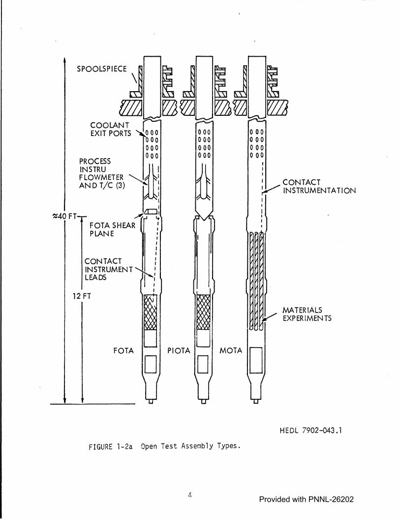
ECFMs are present in two different configurations: The Open Test Assemblies (.OTA), which have long instrument stalks extending above the core, have their ECFMs inside the instrument stalk and provide very accurate flow measurements, (see Figure 1-2) Fuel Driver Assemblies and reflectors do not extend beyond the top of the core, rather they terminate with a handling socket. The ECFMs in this case are in an instrument tree which is placed above the core. Figure 1-3 shows the two types of configuration in the FFTF.


FTR CORE MAP

Figure 1-1 Placement of ECFMs with Phase-Sensitive Detection Electronics for FFTF Acceptance Testing.

3

N

I


SPOOLSPIECE j fZl1

COOLANT EXIT PORTS

PROCESS INSTRU I FLOWMETER ..........._ IA I

AND T/C (3) ' : I I I

~40FT ~LCJ~ FOTA SHEAR 1

I PLANE I

I I I I

CONTACT / INSTRUMENT 'th..' LEADS I f

I 12 FT

!J rJ~

FOTA PIOTA

0 00 0 00 0 00 0 00

D D

J VJ

0 0 0 0

! w

00 00 00 00

1 CONTACT V INSTRUMENTATION

MATERIALS EXP ER IMEN TS

MOTA D

HEDL 7902-043. l

FIGURE l-2a Open Test Assembly Types.


01

FUELS OPEN TEST ASSEMBLY (FOTAJ

RETAINING PLATE

HOLDDOWN RING

FOTA STALK ASS'Y

INSTRUMENTED FUEL ASS'Y

ELECTRICAL CONNECTOR

PRESSURE TUBES

HCDA RETAINING TUBE ASS'Y

SPOOL PIECE

CLOSURE HOLD -DOWN MECHANISM

INSTRUMENTATION LEADS

TOP CUTTER HEAD

ELASTOMER 0-RINGS

REMOVABLE INSTRUMENT ASS'Y

BULKHEAD

LOCK TUBE

CUTTER GUIDE TUBE

I _.l_.)l-...W---A...J ____ /J

L---~ FIGURE l-2b Fuels OPEN TEST ASSEMBLY (FOTA)

r·---1 I ;·

i i ! i:

I

1·

I I

HEAD BOLTS

SPOOL PIECE TO HEAD MECHANICAL SEAL -r----<iil

REACTOR HEAD

BULKHEAD

BULKHEAD

MECHANICAL SEAL

LOCK TUBE


FUELS OPEN TEST ASSEMBLY ( FOT A) CONTINUED

SHIELD WAFERS

I i' I SPOOL PIECE

f~~-. BULKHEAD

---I-HEAD

·1'.~ '~I

I I FOTA STALK ASS'Y ~ , I ---- ------ -----.:.---- -

INSTRUMENTED FUEL ASS'Y

/ /

/ /

FIGURE l-2b (Continued)

VI

! I

I.

i: I

I

'I

I:

; !

--- -

I

'I

'li 'I

111

r:: ,1

11

I, i,

BULKHEAD

CUTTER GUIDE TUBE

LOCK TUBE

COOLANT OUTLET PORTS !TYPICAL 4 ROWS)

I

TAPERED FLOW PLUG

__.-,-"] /' -- I

"'

i I i ·---

i:I -~

lb -

~l ' 1!

-~ : i t:. , ---THERMOCOUPLES

"' ~ ,~','I [.~l I L- FLOWMETER

i ' i v f"-

1- FLOWMETER I/ '.£-~ WELL

'-~

I

! IL

I LOCK TUBE L-

1i

r L-- HANDLING ~ SOCKET

--~~

~IV HEDL 7409-59.2


EXPERIMENTER CONTACT INSTR LEADS ~

PROCESS INSTR PACKAGE

FOTA SHEAR PLANE

FUELED REGION

>-VI VI <(

...I w ::> u..

<( ,_ 0 LL

"" 3: 0 "'

>- >-VI VI VI VI <( ' <(

..J I <( ..J w I I- w ::> ,o ::> u.. 'u.. LL

M "<t · IO

3: 3: 3: 0 0 0 "' "' "'

CORE BASKET

>- >-VI VI V'l VI

<( <( <(

0 ..J ..J u.. u.. w w ... "' "'

~ co

'° " ~ "'

~ "'

FIGURE l-3 Schematic of Typical OTA Core Arrangement.

7

TOP OF OTA 39.9'

TOP OF HEAD 32.9'

BOTTOM OF HEAD 31.1'

TOP OF SODIUM 28'

q; TOP SLOT 19.5'

q; BOTTOM SLOT 17'

TOP OF CORE 12'

-----0

f.i EDL 7902-043. 12


2.0 HARDWARE DESCRIPTION

This section presents a physical description of the ECFM and the associated electronics, both AD and PSD. In operation the ECFM is placed in a stainless steel thimble which isolates it from the sodium. The thimble is oriented with respect to the flow such that the flow is along its axis.

2.1 ECFM

The ECFM consist of three coils placed on a single axis inside a steel container (see Figure 2-1). The middle coil in this configuration is the primary coil and the other two are secondary coils. The secondary coils are connected to provide an output which is the difference of the two induced EMFs. The physical properties of the ECFM probe were specified in Standard RDT & C-4-7, Reference 5.

2.2 Amplitude Detection Electronics

The AD electronics consist of two basic modules. One module contains the system power supply and a master l KHz oscillator. The second module contains a signal conditioning (SC) circuit and a current regulating (CR) circuit which provides a nominal 0.5 ampere a.c. drive current to the primary coil of the ECFM. The power supply and oscillator provide power and signal to operate six SC/CR modules housed in a standard 19u NIM Bin and are themselves housed in a standard 19 11 NIM Bin along with two more power supply/oscillator packages.

The power supplies are standard items manufactured by Lambda Electronics Corporation of Melville, New York. Details of the specificatiofis for these

modules are fncluded 'in Operati:ons Mai'ntenance Manual, OMM~092-00-002, Volume. 1 and Standard RDT & c~10~5, Reference 6.

The SC/CR (see Figure 2-2) provides a "constant current" a.c. sine wave of 0.5 amperes rms amplitude at l KHz frequency to the primary coil of the ECFM. The CR (essentially a non-inverting feedback amplifier) is excited by the output of the oscillator in the power supply/oscillator module. The SC section of the module has three basic circuits: 1) the differential

·8 Provided with PNNL-26202

FIUGRE 2-1 Photograph of a longitudinal cross section of an Eddy Current Flowmeter. The instrument lead enters at the top of the figure, where three thermocouples are located. Paired primary and secondary coils are wound around the hollow central shaft which occupies most of the picture. The truncated leads to the primary (the middle two wire pairs) and secondary (the outer pairs) coils are seen in this hollow central shaft. At the bottom of the picture is the stainless steel ogive which caps the stainless steel jacket surrounding the thermocouples and the flowmeter coils.


FIGURE 2.1 9 Provided with PNNL-26202

FIGURE 2-2 Signal Conditioner/Current Regu1ator Module

10


amplifier/bandpass filter, 2) the a.c. nulling circuit and 3) the detector circuit. Emf imbalances from the ECFM secondary coils are amplified, filtered

and the internally generated signal from the a.c. nulling circuit is used in the summing amplifier to remove any residual biases. Figure 2-3 provides a schematic summary of the action of the SC/CR in providing the d.c. output from the coil imbalances.

The test calibration station (see Figure 2-4) incorporates the capability for testing every function of the system. It contains a built-in Fluke digital voltmeter which makes all measurements and it is designed to operate in conjunction with or independently of the flowmeter system as the station incorporates its own power s.upplfes. The station also fncorporates i.nternal circuitry and a test s.witch which provides the station with a self-test capability. In operation, the station is capable of checking the ECFM by either taking d.c. resistance measurements or actual flow readings. The station, further incorporates an ECFM simulator circuit which allows for

simulation of the zero flow condition for an ICFM.

The zero flow signal is utilized in calibration. checkout, or adjustment of a SC module at full load by connecting the SC module to the test station. Any SC module can be adjusted to a specific ECFM via the procedure of simulating zero flow independent of the actual state of the system.

The test station also has the capability for checking the output of any power supply.

2.3 Phase-Sensitive Detection Electronics

The PSD electronics differ from the AD electronics in that they make use of only the CR aspects of the SC/CR and the differential input amplifier high pass filter (See Figure 2-3). This modification bypasses most of the SC module. Typical circuitry for this 11 piggy-backed 11 system is shown in Figure 2-5. While the AD circuit is not shown here, it remains intact and the PSD system is added on to expand the capabilities of the ECFM.


NULL NG r----.J'.rv'----~ --

CURRENT REGULATOR

........ zz ~I,.., .... a: l/) a: z :::, Ou u

CIRCUIT

SUMMING AMPL. A~:D LOW PASS FILTER

>----1DETECTOR1---

AVERAGING DIFF. INPUT ~1 L TE R AMPLIFIER &. HIGH F'ASS FILTER SIGNAL CONDITIONER

!!

THIMBLE

.....__.......__~.,..____,.....__......__._.,--..__...._~-__. EDDY CURRENT FLOWMETER PROBE

SECONDARY COi L

.__ FLOW DUCT

t t ~ , ' t FL.OWING SODIUM

12

FIGURE 2-3

FUNCTIONAL BLOCK DIAGRAM . OF A SINGLE ECFM CHANNEL


__. w

---- ---- ----------------------------------------------,

t;,.\!t a . ;. ,. .

.. f

'.ti "' ... 'f';')! .:,flt(:

~'..9 ... ... .

. :, . -. '.J

·~ ,_.,.

1 •-.I'-'

0 ,:a2,:·

•• l::t)Nf-'~

·H,. -~ OH ~.'O•

FIGURE 2-4 Test/Calibration Station

t.Cr\l 'inU'llAilOA ... . ... • . . e··

C0Ali~4. c,.,i. .• r '\:ro.1

•. "":~ •

~

TEST CALIBRATION STATION

•Cftl 11'$T WUCT -


CURREt\T REGU~A~o;;,

LOCK-IN AMPLIFIER

0N orW/0

90° PHASE SHIFT)

~_.... ATTENUATOR

o·Fc: INPUT At-JP L I F I E R Y' GH FASS FILrER

THIMBLE

OUTPUT

EDDY CURRENT FLOWMETER PROBE

SECONDARY COi L

PRIMARY COIL

SECONDARY COIL

i,--.--FLOW DUCT

/

FLOWING SODIUM

14

FIGURE 2-5

FUNCTIONAL BLOCK DIAGRAM OF A SINGLE ECFM CHANNEL


Several components are common to both systems; namely, the CR, the differential input amplifier/high pass filter and the test calibration module. The ad~itional components used in PSO are a lock-in amplifier and an ohmic attenuator to provide appropriately scaled inputs for the amplifier.

The PSO electronics are of two types: The first, used on all subassemblies except the Row 2 FOTA (HFOll), employs a Princeton Applied Research (PAR) Model 128 A Lock-In Amplifier (see Figure 2-6) to provide the flow signal output using the typical circuitry in Figure 2-5. The Row 2 FOTA employs a PAR Model 5204 Lock-In Analyzer (see Figure 2-7) which is basically two lock-in amplifiers with a go0 phase difference between the two channels. The output of this analyzer consists of two signals: one being the usual flow signal, the other being the component of the signal go 0 out-of-phase with the flow signal. Analysis of PSO measurement theory in Section 3 explains the value of this configuration and of PSO itself for low flows.

The physical characteristics of the two lock-in amplfiersare detailed in Appendix A.

As a final hardware note, the calibration program employed PAR Model 120 Lock-In-Amplifiers which differ substantively in that they have a 20 mv setting, on which all calibration was performed, while both models used in the FFTF have a 25 mv setting. The differences are compensated by adjusting the resistance of the attenuators as described in Section 5.2.

,~ Provided with PNNL-26202

FIGURE 2-6 PAR Model 128A Lock-In Amplifier The Princton Applied Research (PAR) Model 128A Lock-In Amplifier (Front View) is used for all ECFM flow evaluation by PSD except HFOll. Specifications are presented in Appendix A.


It • ; •

0 0

FIGURE 2-7 PAR Model 5204 Lock-In Analyzer The Princeton Applied Research (PAR) Model 5204 Lock-In Analyzer used by HFOll in FFTF Acceptance Testing. This analyzer acts as two LocR-In Amplifiers. Specffitattons are given in Appendix A.

l 7 Provided with PNNL-26202

3.0 ANALYSIS

This section presents a simplified version of the theory of ECFMs. Both AD and PSD are described in order to provide the motivation for PSD. Error sources are very important in any measurement technique and Section 3.4 presents a discussion of several error sources which are present in flow measurement. Finally Section 3.5 reports the results of the calibration program and discusses errors remaining in the flow signal.

3.1 ECFM

A detailed discussion of the theory of operation of the ECFM is presented in both Appendix Band in Reference 7. Figure 2-3 provides a schematic picture of the operation of an ECFM immersed in flowing sodium.

An alternating current (in this case 1000 Hz) is applied to the primary coil. The choice of frequency is influenced by the conductor resistivity, the use a thimble (dry) or director immersion (wet), and considerations such as lead-to-lead coupling in the electronics. The sodium penetration decreases with increasing freauency and at 1000 Hz the thimble alone attenuates the s i gna 1 by 40%. · ( See Refernce 8.) The a 1 ternati ng current flowing in the primary induces eddy currents in the sodium which, when the sodium velocity is zero, are parallel to a plane normal to the axis of the coil, symmetric with respect to the plane in magnitude, but flow in opposite directions. If the sodium has a velocity along the axis of the coil, then the upstream eddy currents develop a damping term which is essentially bilinear in velocity and conductivity, thus introducing a skew in the EM field in the direction of flow. When the eddy currents are imbalanced by the sodium flow, a different emf is induced in each of the secondary coils. The difference in the two emfs becomes the flow signal.

There are some problems involved, in that this signal has non-flow components which arise from the variation in sodium conductivity with temperature, thermal changes in the coils (both secondary and primary), variations in permittivity of the thimble and the sodium etc. The dominant temperature variation in the non-flow component is usually the conductivity of the sodium although changes in the thimble and the environment tan bi~s the low flow values in both phase and amplitude.


The sum of the secondary coil emfs will contain the same information except that, to first order, the flow dependence will be eliminated. Thus the temperature dependence of the signal is enhanced. This fact has been used to provide a correction for the temperature effects and improvement in the linearity for linear variable differential transformer (LVDT).

(See Reference 9). In fact, when the sum of the emfs is used, it is possible to use the ECFM as a high speed temperature measuring device with good accuracy (5°F). Reference 10 is a series of papers on just this topic.

3.2 Amplitude Detection This technique of flow measurement assumes the non-flow components are

not important and ignores the Phase,•, of the flow signal. The first assumption of AD is that, while there is temperature dependence in the flow signal, all flow lines cross at a single.point, S, in an amplitudephase (v-•} plot at the point corresponding to zero flow.

The second assumption is that S also corresponds to the origin of the v-• plot. Thus the assumed form of av-• plot is that pictured in Figure 3-1.

It is clear from examining this figure that the amplitude (distance from the origin) of the flow signal for a fixed flow is independent of the temperature and vanishes when the flow vanishes. When one assumes the relationship of flow to signal is linear (a very good assumption in this case) only a gain is necessary to convert the flow signal to appropriate flow units.

In fact, both assumptions are violated to some extent by real ECFMs. Figure 3-2 represents typical v-• plots for ECFMs. In Figure 3-2a the flow signals have all erased at a single point, S, but it is not the origin and it is not zero flow. Had it been zero flow, one could have translated the origin to the zero flow point and obtained Figure 3-1. The AD calibration procedure translated the origin to zero flow rather than to S. Either of these choices seems to be on equal footing, and nulling the amplitude at zero flow is easier than measuring from S (which first must be determined). The consequences of the two choices are shown


X = V AC cos fl)

y = VAC S1N4'

ARBITRARY UN ITS

y

FIGURE 3-1 IDEAL ECFM Amplitude-Phase Plot

20

X

ARBITRARY UNITS

HE DL 7902-043. Provided with PNNL-26202

y

6

5

4

3

ZERO FLOW 2

-5 -4 -3

x = V AC COS()

y = V AC SIN cf>

~ -2

-4

ALL LINES INTERSECT AT (1, 1)

1 2

FIGURE 3-2a Realistic ECFM Amplitude-Phase Plot

21

T5 T4 T3 T2 T1

3 4 5 )(

HEDL 7902-043 .2


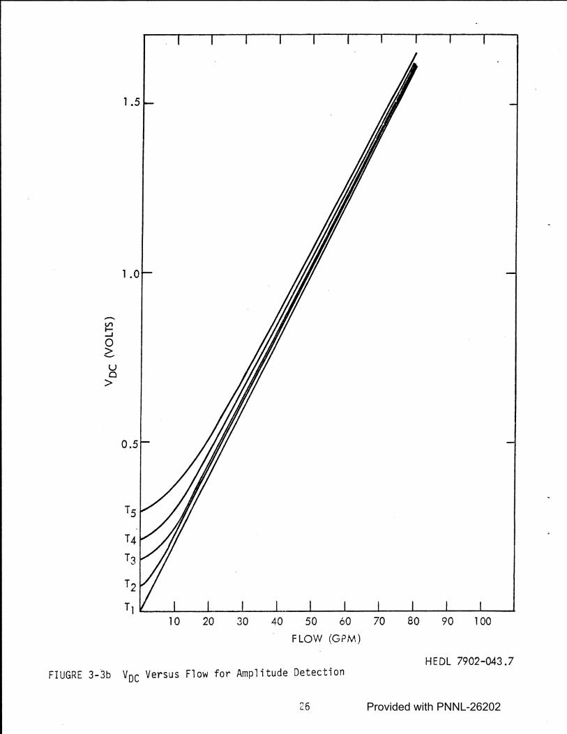
in Figure 3-3a. Note that nulling to zero flow has produced a family of curves, whereas measuring from S has produced on straight line with a non-zero intercept. When nulling to zero flow, one is given the impression that some nonlinear, temperature-dependent, flow-dependent effect is entering at low flows. It is in fact just an artifact of the nulling process.

If there were no point S, one could get two distinct types of situations, Figure 3-2a and 3-2c, which correspond to Figures 3-3b and 3-3c when one examines the flow signal versus flow. Type b could be improved somewhat by measuring from an approximate S value, however, Type C is double valued! Nothing can be done to resolve the ambiguity at low flow using AD. Note that if the AD were to null to Sin Type b a double-valued result would result.

Use of AD for higher flow is quite reliable, but the matching of the secondary coils in the ECFM is not done sufficiently well to use AD in the low flow regime. Moreover, it may not be feasible to perform matching to the level of accuracy required by low flows.

3.3 Phase-Sensitive Detection

PSD was instituted on several ECFMs at the FFTF to ameliorate the difficulties caused by the inability Of AD-calibrated ECFMs to provide the necessary low flow data. PSD, in essence, measures the distance from a line perpendicular to the reference flow line {usually 400°F) and calculates the flow from the quantity. Ideally a flowmeter should be such that the flow lines for different temperature never cross. This means that the line perpendicular to the reference flow line is perpendicular to all flow lines and the distance from the line is dependent only on flow, not on temperature.

If the ideal situation were obtained, then while the flow measurements would have no temperature dependence, the change in the distance from the origin to the flow line {an easily obtained quantity) would be dependent only on the temperature. Thus it could act as a high-speed, high accuracy temperature measuring device with little post-processing of the signal.

There were approximately 140 ECFMs available at HEDL which had been calibrated using AD. For each flowmeter a complete file of VAe and 9


-2.0 -1.5

x = vAc cos c:,

y = VAC SIN 4>

NO COMMON INTERSECTION POINT (NOTE SCALE CHANGE)

FIGURE 3-2b Realistic ECFM Amplitude - Phase Plot

23

y

1.5

0.5 X

-0.5

-1.0

HEDL 7902-043 .4


1.5

1.0

0.5 ZERO FLOW

-1.0 -0.5

-0.5

-1.0

FIGURE 3-2c Realistic ECFM Amplitude - Phase Plot

24

1.0

x = v Ac cos 4>

y = VAC SIN 4)

X

HEDL 7902-043.


2.0 V DC

1.5

1.0

-0.5

-1.0

10

/ /

/

--- ___ NULL TO SAND CARRY SIGN

/ /

/ /

/

/ /

20 30 40 / 50 60 70 80 90 100

FLOW (GPM)

/ /

/

/ /

/ /

/

FIGURE 3-3a v0C Versus Flow for Amplitude Detection

HE DL 7902-043. 6


-I!? -I

0 c. u C

>

T4

T3

T2

T1 L..-~.J.....~-1...~.....1.~~1....-~....1-..~-.1...~___i.~~L....~..l._~....L.~....J

10 20 30 40 50 60 70 80 90 100

FLOW (GPM)

HEDL 7902-043.7 FIUGRE 3-3b Voe Versus Flow for Amplitude Detection


-V> 1-...J

0 > -u 0

>

1.5

1.0

0.5

T3 T5

T4

T2 T1 l!..---..l.----'-----L-----l----..L----L-----1------1-----i

10 20 30 40 50 60 70 80

FLOW (GPM)

FIGURE 3-3c Voe Versus Flow for Amplitude Detection

HEDL 7902-043.10 27 Provided with PNNL-26202

was available. Selection of ECFMs far use in low flow measurement was based on the criteria that the fixed low-flew line and the fixed temperature reference line be nearly orthogonal and that the data scatter be minimal.

In order to set up the perpendicular line using PSD, two flows Cat a minimum) must be measured to find their in-phase (Il and quadrature (Q)

components at each flow. The I and Q components are at 90° to one another so that the amplitude (VAcl from the origin (_as opposed to VDC' the amplitude from the zero fJow reference temperature point) is related to the two components by,

1/2 V AC = (12 + Q2}

Any two flow measurements must gfve the same value for Q if Q is to

{3.l)

represent the perpendicular distance from the origin to the flow line. Figure 3-4a shows this situation for two flows w1 and w2. Figure 3-4b shows the case in which the two Q-components are not the same. They are measured along the same direction but they are of different length. The solution is to rotate the direction of measurement of the Q-component by an angle (.0)

until the Q-components at both are equal. (See Figure 3-5.) The angle between the Q-component and the line along which VAC is measured is called a. Therefore, for Q1 to be equal to Q2,

VAC Cos (al +a)= VAC Cos (82 + a). l 2

(3.2)

The unknown voltages VACl and VAC2 are eliminated by the relationship,

In= VAC Sin an. n

(2.3)

Using the angle sum formula for cosines and Equation 3.3 gives,

11 (cot s1 cos a - sin a)= 12 (cot s2 cos a - sin a) (3.4)

or 1 o, - Q2

e = tan - (1 _ 1 ) . l 2

{3.5)

Fr·om the two flows one can ascertain the proper Q-component, which is obtained by changing the measurement angle by an amount e. The new Q is,

Q = VAC Cos (s1 + e) l

28

(3.6)


' ' ' ' ' ' v AcO) ,

'

FIGURE 3-4a Relationship of V and Q for Two Flow ReadingsA~hen Q has bee Properly Adjusted.

FIGURE 3-4b Variation of Q with Flow When Q has hot been Properly Adjusted.

H E DL 7902-043 • 11


'~----Q(l)

' VAc(l~

FIGURE 3-5 Rotation of the Direction of Measurement of Q oy an Angle e to Make Q Flow-Independent.

HEDL 7902-043. 9


which, making use of Equation 1.3,becomes

Q = ~ Cos (a1 + a) (3.7)

In Figures 3-4 and 3-5 one flow point is on either side of the quadrature vector. A more common occurrence is to have both flow points on the same side of Q. The procedure for finding Q is unchanged, however the readings obtained in this case will seem hard to interpret at first glance. A valuable tool for avoiding this confusion is the graphical method. This method gives an approximate value for Q which can be used to verify the more precise algebraic solution outlined above.

Plot the flow point, given by the guadrature and in-phase components for each flow on a Q-I grid. Connect the two flow points with a straight line. A line from the origin, perpendicular to the flow line, is the correct Q. Figure 3-6 shows the graphical method.

Errorarisingfrom the fact that the flow lines do cross one another are small, because the correction is dependent on the sine of the crossing angle, which is small. Thus all of the realistic cases in Figures 3-2 can be treated with a high degree of accuracy using PSD.

3.4 Error Sources

In addition to the errors introduced by the lack of an ideal ECFM (which may be processed out) there are certain error sources which can give rise to e?·rors that limit the ultimate accuracy of the flow measurement. There are three basic sources: (1) hardware-related biases, (2) electronicsbiases, and (3) noise,each of which will be discussed in the next three sections.

3.4.l Hardware Biases

This category of biases includes the thimble related environment changes, the sodium channel changes, wire routing changes, etc. The net effect of these changes is to alter VAC and~ in such a fashion that a rotation and a shift of the flow/temperature grid on the v-¢ plot occurs. The sensitivities (!~and~~) can be affected by these changes. When the ECFM is setup in the FFTF, only two flows are required and if one is known (i.e., zero flow), the shift and rotation of the flow/temperature grid can be processed out during the setup. The sensitivity changes, though small, will remain.


' ... ' ' ' Q(l ), I(l)

' ... ' ' .. ,

I (VOLTS)

I(1)

' ... ' ' Q(2), 1(2)

I(2) ' ' '

Q(l) Q(2)

FIGURE 3-6 Graphical Method for Obtaining Q. Th.e length Qt is an estimate of the correct quadrature Q, given two sets of measurements [Q(l), I (J) ] and [Q(2)., I (2)], at different flows. The new coordinate system is obtained by rotating the old system until the Q value becomes Ql. The rotational angle will be determined better at flow #1, because r Q ( l) - Q I I > ' jQ(2) - Q' j. After rotation,. all Q~yalues will be constant.

32

' ' ' ' ', FLOW LINE

' ', Q (VOLTS)

HEDL 7902-043 .8


3.4.2 Electronics Biases

After the calibration program, variations in the electronics components were observed (see Table S-1). In the calibration program a PAR Model 120 lock-in amplifier was used in conjunction with external attenuation and Signal Conditioning/Current Regulator Modules (SC/SR), the latter being calibrated to plant specifications. (See Reference 10.) The variations in the components are scaled by the input voltage column and renr~c:,rnt a small error on the· order of l/4 GPM at zero flow. In plant calibration includes compensation for these variation. In effect the sensitivities (;~ and :i) are also perturbed, but again, only very slightly.

3.4.3 Noise

The TTL facility and the recording apparatus constitute a generator of random signals of a variety of frequencies and amplitudes. An analysis of the noise on the measured data is probably the best estimate of this error.(see next section). It will be present in the FFTF .as well as the TTL.

3.5 Calibration Results

This section presents a sunmary of the results of processing the ECFM calibration runs at the TTL using the PSD. The discussion addresses the biases which arose in repeat runs when the test thimble and the electronics were changed, the noise level on the data and the flow/temperature calibration curves for each ECFM. For S/N 172, which is in the Row 2 FOTA and has both I and Q output, both the temperature and flow calibrations are reported.

The ECFM response obtained in the TTL may differ from the ECFM response I

in the FFTF. The effect on the calibration curve can be expressed in terms of the changes which can occur in the v-~ plot. Three separate changes to the calibration grid can occur: (1) it can be rotated around the origin in the v-~ plot, (2) it can be scaled and (3) it can be translated with respect to the origin.

The rotation is easily adjusted out during the setup of the quadrature. The scaling has not occurred during test station changes at TTL and is not expected to enter in any significant way.


The translation with respect to the origin has occurred during testing at the TTL. When the quadrature vector is adjusted, there is a residual difference between the length of the in-phase vector at zero flow in the two cases. Such differences will almost certainly occur when the ECFMs are calibrated in the FFTF. Two solutions present themselves: (l) select zero flow for one of the two flows used in the setup and establish procedures for obtafnfng zero flow, or (21 use a Kalman ftlter to proces·s out tfle bias in tbe flow data after-tne-fact.

3.5.l Calibration Curves

The summary of the flow calibration curves for the ECFMs calibrated at the TTL are presented in Tables3.l to 3. 15. These curves are functions of both temperature and flow. While the voltage biases for each run are included, the absolute bias is a function of many variables and will be redetermined in the plant. The temperature sensitivity of the bias is also a function of the environment.

The calibration curves are straight lines and satisfy;

Flow= (Voe ~ Bias)/Slope

where v0C is the in-phase component I,

Slope= Sl + S2 ~ T,

and

Bias= Bl+ 82 · T

(3-8)

(3-9)

(3-10)

The values of Sl, S2, Bl and 82 are included in Tables 3.1 to 3.15. Several tables show different signs for Sl fordlfferent runs. This is a result of the relative phase setting on the lock~in anplifier and as a matter of convention all of these parameters are multiplied by the sign of Sl. Table 3.16 is a summary of paral'!Bters. Note that all of the parameters listed in Table 3.16 are scaled by a factor of 10. This difference is due to a change in amplifier gain between the TTL and the FFTF. As described in the next paragraph, several runs were discounted because of obvious data acquisition errors.


Table 3.1

i S/N 052 Parameters

Run #1 T°F Bias (V) Slope (V/GPM) RMS (GPM)

400.0 .404926 . 030161 .504612 500.0 .348626 .030347 .512748 600.0 .294221 .030197 .579480 700.0 :242743 .029889 .510724 800.0 .258666 .030155 .322982 900.0 .187046 . 0297,54 .602076

1000.0 .094759 .028569 . 368891 1100. 0 -.009830 .027804 .379466

Bl = .627486 Sl = .031972

82 = -.0005331223 S2 = -.0000031496


400.0 . 726265 .030086 .161921 600.0 .649766 .030529 .223428 700.0 .610819 .030238 . 167526 800.0 .563427 .030038 . 197729 900.0 .535142 .029281 .174214

1000.0 .486676 .029423 . 139064 1100. 0 .462778 .028033 .216970

Bl= .878950 Sl = .031860

82 = -.0003850504 S2 = -.0000027984


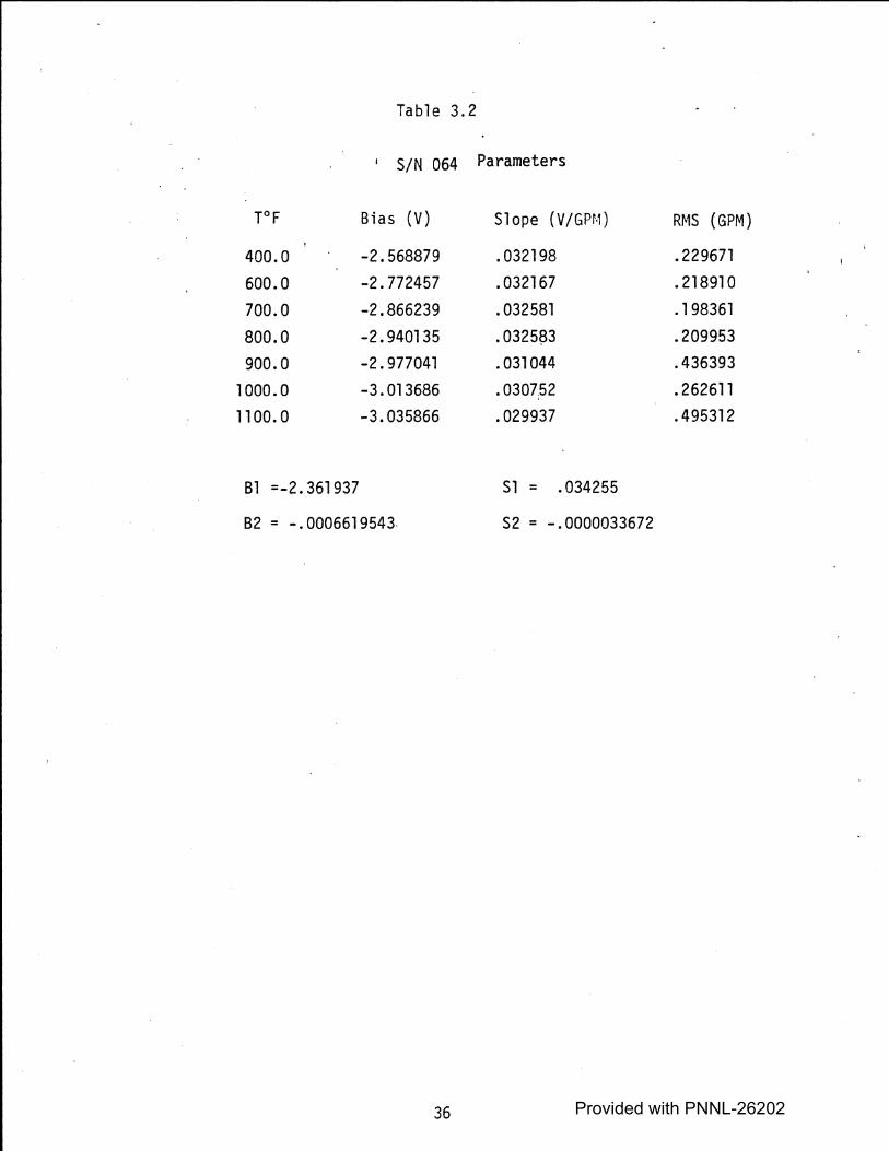
Table 3.2

I S/N 064 Parameters

T°F Bias (V) Slope (V/GPM) RMS {GPM)

400.0 -2.568879 .032198 . 229671

600.0 -2.772457 .032167 .218910

700.0 -2.866239 • 032581 .198361

800.0 -2.940135 .0325~3 .209953

900.0 -2. 977041 .031044 .436393

1000.0 -3.013686 .0307.52 . 262611

1100. 0 -3.035866 .029937 .495312

Bl =-2.361937 Sl = .034255

82 = - . 0006619543. S2 = -.0000033672


Table 3.3

j S/N 078 Parameters.


400.0 2.1S8090 -.031698 -.218712 600.0 2.241499 -.032069 -.192551 700.0 2. 184301. -.031365 -.260619 800.0 2.126020 -.031545 -.232035 900.0 2.152527 -.030803 -.357274

1000.0 2. 332331 - . 030.313 - . 848971 1100.0 2.480885 -.029544 -.342618

Bl = 1.999355 Sl = -.033570

82 = . 0003109407. S2 = .0000032093


400.0 2.146267 -. 031146 -. 106323 600.0 2.245697 -.031372 -.162133 700.0 2.273608 -.031151 -.163994 800.0 2.283862 -.031305 - . l 02806 900.0 2.261030 -.029935 - . 327723

1000. 0 ,2.229798 -.029733 -.209881 1100. 0 2. 179137 -.028967 -.378781

Bl= 2.199941 Sl = -.033144

82 = .0000399663 S2 = .0000033454


Table 3.4


Run #1 T°F Bias (V) Slope (V/GP~1) RMS (GPM)

400.0 .410214 .032570 .222756

600.0 .398231 .033076 .255634

700.0 .396138 .032933 .236419

800.0 ~393234 • 032531 .285982

900.0 .381666 . 032131 .152998

1000.0 .395459 .030983 .245714

1100. 0 .392174 .030308 .302498

Bl = .415375 Sl = .034841

B2 = -.0000255475 S2 = -.0000035194

Run #2 T°F Bias* (V) Slope* (V/GPM) RMS* (GPM)

400.0 . 103007 . 018785 .202367

600.0 .083521 .018436 .401982

700.0 .036582 . 018577 .541246

800.0 -.034214 .018064 .149819

900.0 -.029699 .017627 .744082

· 1000. 0 • 120951 .017115 1. 185363

1100. 0 . 177189 . 016776 1.053693

Bl= .021728 Sl = . 020277

B2 = .0000554978 S2 = -.0000030103

*An extra 5,l(Q resistor in the circuit introduced a factor of o·.6 in this run.


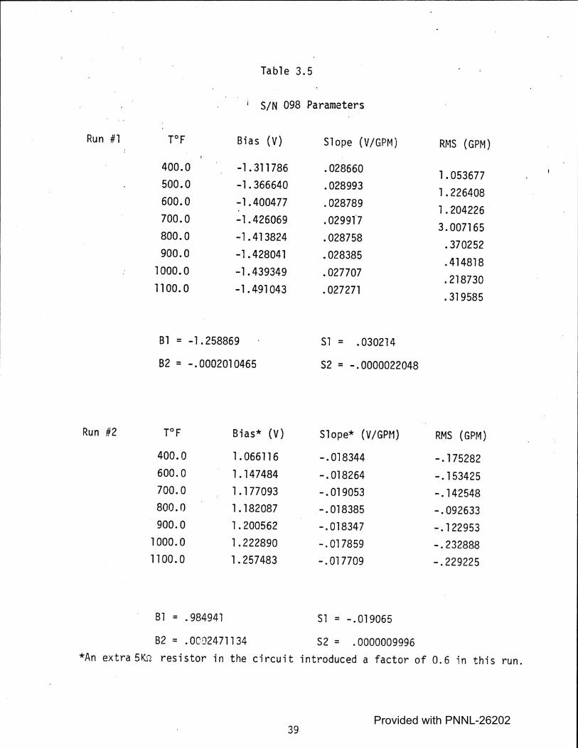
Table 3.5

S/N 098 Parameters

Run #1 T°F Bias (V) Slope {V/GPM) RMS (GPM)

400.0 -1. 311786 .028660 1. 053677 500.0 -1.366640 .028993 1.226408 600.0 -1.400477 .028789 1.204226 700.0 -1.426069 . 0299l7 3.007165 800.0 -1.413824 .028758 .370252 900.0 -1.428041 .028385

.414818 1000.0 -1.439349 .027707 .218730 1100.0 -1. 491043 • 027271 .319585

Bl= -1.258869 Sl = .030214

B2 = -.0002010465 S2 = -.0000022048

Run #2 T°F Bias* (V) Slope* (V/GPM) RMS (GPM)

400.0 1.066116 - . 018344 -.175282 600.0 1. 147484 -. 018264 -.153425 700.0 1. 177093 -.019053 -. 142548 800.0 1.182087 -.018385 -.092633 900.0 1.200562 -.018347 -. 122953

1000.0 1.222890 -.017859 -.232888 1100. 0 1.257483 -.017709 -.229225

Bl = .984941 Sl = -.019065

B2 = .0002471134 S2 = .0000009996 *An extra 5Kn resistor in the circuit introduced a factor of 0.6 in this run.


Table 3. 6


T°F Bias (V) Slope (V/GPM) RMS {GPM)

400.0 .064128 .031058 .185080 600.0 .082627 .030825 .156914 700.0 .079259 .030689 . 233051 800.0 .086858 .o3o4i4 .318283 900.0 . 106634 .030055 .508100

1000. 0 . 166253 .0290,39 .292469 1100. 0 . 188966 .028874 .347757

Bl= -.028108 Sl = . 032769

82 = . 0001766325, S2 = -.0000033496


Table 3. 7


Run #1 T°F Bias (V) Slope (V/GPM) RMS {GPM)

400.0 -.715633 .030730 .482525 600.0 -.814390 .032592 .354225 700.0 -.843053 .032730 .521336 800.0 :..878454 .032705 .799776 900.0 -.942039 .032877 .684958

1000.0 -1.048316 .033717 .651696 1100.0 -1. 190856 .034785 .674861

Bl = -.424000 Sl = • 029110

B2 = -.0006299533 · S2 = .0000047936


400.0 -.517290 .031326 . l 06633 600.0 -.433507 .031325 . 173329 700.0 -.383485 . 030671 .216978 800.0 -.348473 .030742 .233291 900.0 -.305033 .030165 . 175701

1000.0 -.268285 .029655 .231682 1100."0 -.193402 .028739 .190746

Bl = -.698843 Sl = .033206

B2 = .0004440772 S2 = -.0000036031


Table 3.8 ·

j S/N 128 Parameters


400.Q .747313 .028916 • 149029 600.0 .839853 .029053 .176245 700.0 .892686 .028328 .213210 800.0 : 920184 • 028088 .248617 900.0 .956047 .027646 . 285951

1000. 0 .989685 .027294 • 155110 11 oo. 0 1. 046236 .026563 .276405

Bl = .591794 Sl = .030732

82 = .0004089895 S2 = -.0000034972


400.0 .516283 .030220 . 152294

600.0 . 599973 .030503 .248662 700.0 .654381 . 030121 .333847 800.0 .691739 .029823 .210730 900.0 . 725340 .029425 .171227

1000.0 .746044 .029018 .229188 1100. 0 .789418 .028160 .222994

Bl = .372474 Sl = • 031967

B2 = .0003847023 S2 = -.0000029992


Table 3.9

j S/N 156 Parameters


400.0 -1. 013324 .029825 .202318 600.0 -1.009467 .029705 .292939 700.0 - .998643 .029732 .255655 800.0 ~ .986815 .0297~2 .187907 900.0 - .955683 .029250 .236706

1000.0 - .934050 .029047 .294872 1100.0 - • 912731 .027993 .292973

Bl = -1. 093765 Sl = .031086

82 = • 0001537525. S2 = 0.0000022345

Run #2 T°F Bias {V) Slope (V/GPM) RMS {GPM) 400.0 -.826294 .028951 . 189323 600.0 -.798583 .029287 . 188993 700.0 -.766750 .029135 .203400 800.0 -.733726 .028763 .252994 900.0 · -.693084 .028374 . 191550

1000.0 -.645439 .027620 . 184455 1100.0 -.6092J5 .027029 . 181090

· Bl = - • 980050 Sl = .030786

82 = .0003249526 S2 = -.0000029715


Table 3.10



400.0 -.334092 .030159 . 178307

600.0 -.323246 .030187 . 172948

700.0 -.312447 .029578 .248640

800.0 .:...304404 .029603 .222979

900.0 -.286557 .029105 .422616

1000.0 -.283594 .028865 .• 626448

1100.0 -.268628 .027740 .670678

Bl = - • 377100 Sl = .031847

B2 = .0000957699 S2 = -.0000032175


400.0 -.506052 . 030641 . 197586

600.0 -. 528715 .030659 . 166237

700.0 -. 512115 .030574 .232369

800.0 -.490360 .030323 .234835

900.0 -.528134 .030240 .474143

1000.0 -.554172 .029015 .343209

1100. 0 -.560294 .028459 . 311398

Bl = -.469497 Sl = .032426

B2 = -.0000715208 S2 = -.0000031041


Table 3. 11

S/N 164 Parameters


400.0 -.931465 .. 029393 . 135195 600.0 -.960698 .029673 • 154130 700.0 -.965268 .029166 .200688 800.0 ·-. 984598 .029088 .238926 900.0 -.976959 .028542 .222246

1000.0 -.921906 .028149 .240597 1100. 0 -.863095 .027371 . 197002

Bl = -1.001817 Sl = • 031105

B2 = .0000743lql S2 = -.0000029735


400.0 -1.238576 .030790 . 185950 600.0 -1.264099 .031049 . 175565 700.0 -1. 261235 .030462 .333368 800.0 -1.266589 .030475 .332485 900.0 -1.269469 .030400 .508013

1000. 0 -1.253502 .029670 .269943 1100.0 -1. 231074 .028796 . 312279

Bl = -1.259242 Sl = .032343

B2 = .0000054818 S2 = -.0000026839


Table 3. 12



400.0 1 • 165144 .023597 .196426

600.0 1. 172185 .023638 .165362

700.0 1.151381 .025190 . 154781

800.0 1.132190 .023827 .101073

900.0 1. 098150 .023856 . 128713

1000.0 1.068585 .023542 . 108390

1100. 0 1.035932 .022705 . 155161

Bl = 1.274438 Sl = .024674 82 = - . 0001995452 S2 = -.0000011578


400.0 1.220693 .032743 . 216341

600.0 1. 234435 .034537 .531979

700.0 1.239034 .033577 .238634

800.0 1.236476 .032913 . 184115

900.0 1.226639 . 031881 .454185

1000.0 1.176964 .031866 .301639

1100. 0 1.109343 .030626 .342830

Bl = 1 .'313488 Sl = .035644 82 = - .0001365151 S2 = -.0000038844


400.0 1. 245072 . 031472 .202183

600.0 1.282226 .031303 .234432

700.0 1.265343 .031024 .233il8

800.0 1.215923 .031303 . 160429

900.0 1.145447 .031380 ·. 528557

1000.0 1.091266 .029388 .406395

1100. 0 1. 023844 .029730 .302421

Bl = 1.458393 Sl = .032913 82 = -.0003526593 S2 = -.0000026885


Table 3. 13



400,0 .148762 .031281 .294969

600.0 .137557 .032008 .302299

700.0 • 136618 .032107 . 334061

800.0 ·. 141750 .032364 .156915

900.0 . 163834 .030361 .359169

1000.0 .. 179851 .031299 .290575

1100.0 .192289 .0303'43 .403654

Bl = .100691 Sl = • 032716

82 = .0000719682 S2 = -.0000016824


400.0 .342747 .031638 .218153 600.0 .352039 .033061 . 191972 700.0 .380906 .032602 .331962 800.0 .445790 .031913 .263979 900.0 .503451 .031648 .354667

1000.0 .395286 .030736 .755003 1100. 0 .246027 .030416 .586130

Bl = .390580 Sl = • 033789

82 = -.0000123296 S2 = -.0000026381


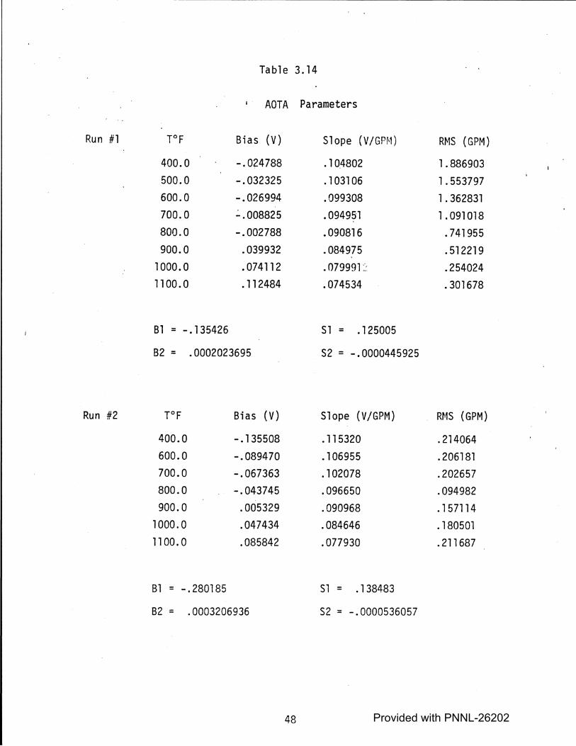
Table 3.14

i. AOTA Parameters

Run #1 T°F Bias {V) Slope {V/GPM) RMS (GPM)

400.0 -.024788 . 10.4802 1. 886903 500.0 -.032325 . 103106 1. 553797 600.0 -.026994 .099308 1. 362831 700.0 .:..008825 • 094951 1.091018 800.0 -.002788 .090816 .741955 900.0 .039932 .084975 .512219

1000. 0 . 074112 . 079991 ::'. .254024 1100. 0 .112484 .074534 .301678

Bl = -.135426 Sl = .125005

82 = .0002023695 S2 = -.0000445925


400.0 -.135508 . 115320 .214064 600.0 -.089470 . 106955 .206181 700.0 -.067363 .102078 .202657 800.0 -.043745 .096650 .094982 900.0 .005329 .090968 .157114

1000.0 .047434 .084646 . 180501 1100. 0 .085842 .077930 .211687

Bl = -.280185 Sl = .138483

82 = .0003206936 S2 = -.0000536057


Table 3.15



400.0 -.580719 .033842 .216978 600.0 -.602511 .034111 . 376711 700.0 -.594228 .033035 .299516 800.0 -.568129 .0316~8 .298276 900.0 -.564002 .032363 .272746

1000. 0 -.537951 . 031391 .234378 1100. 0 -.515972 .030429 .228228

Bl = -.649188 Sl = .036417

82 = . 0001056007 . S2 = -.0000051024

Run #2 T°F Bias (V) Slope (V/GPM) RMS {GPM)

400 .626337 -.032737 -.497113 600 .668855 -.034142 -.327199 700 .671996 -.034292 -.208642 800 .673330 -.034122 - . 145910 900 .662631 -.033580 -.258667

1000 .632122 -.002688 -.190443 1100 .595858 -.029190 -.652081

Bl = .681859 Sl = -.036129

82 = -.0000439791 S2 = .0000040282


S/N

052 064 078 081 098 109 110 128 156 158 164 172 191 194 (AOTA) 201

TABLE 3.16

CALIBRATION CURVE PARAMETERS

Sl (xl0+2) S2 (xl0+7) (Volt/GPM} (Vol t/GMP /°F)

.319 -2.97

.343 -3.37

.334 -3.28

.343 -4.27

.310 -1.94

.328 -3.35

.332 -0.36 • 313 -3.25 .309 -2.60 .321 -3.16 .317 -2.83 .343 -3.29 .333 -2. 16

1.385 -53.61 .363 -4.57

50

Bl (xlO) B2 (xl0+5) (Volts) (Volts/°F)

0.75 -4.59 -2.36 -6.62 -2.10 -1.75 0.26 -2.26

-1.45 -3.06 -0.03 ,. 77

-0.70 4.44 0.48 3.97

-1.04 2.39 -0.42 -0.84 -1. 13 0.40 1.37 -2.45 0.25 0.30

-0.28 3.21 -0.67 0.75


The 400°F to 700°F runs on ECFM S/.Ns 052, 098 and 194 (AOTA} were all run at the same time and the run suffered a computer failure producing two sets of data which led to the anoma 1 o.us behavior in the rms col umn. Run #1 for S/N 110 and for S/N 172 contain bad data also.

3.5.l.l Temperature and Flow Calibration

The ECFM in the Row 2 FOTA (HFOll} is Serial Number 172 and is attached to the Model 5204 Lock-in Amplifier. This amplifier provides both Q and I

output. Simultaneously. A test run {Run 3C) at the TTL using flows of approximately 20 gpm and 200 gpm was used to find the flow and temperature

dependence of tfl.e. Q vector for S/N 1J2. Talil e 3 .11 a fs·p lays the results of " this run, which may be summarized as follows:

I= (Sl + S2 • T) · Flow+ (Bl+ B2 · T) {3-11)

and

Q =(Tl+ T2 ·T) • Flow+ {Cl+ C2 · T) (3-12}

where I and Qare the in-phase and quadrature vectors; Sl, S2, Bl and 82 are given in Table 3.16 for S/N 172 and Tl, T2, Cl and C2 are defined in Table 3.18.

Note that Bl and Cl are both functions of the location of the absolute zero flow and are subject to change. Note also, the factor of 10 scaling between TTL results and those of the FFTF. Thus the values of BT and Cl to be used in the FFTF will be derived from the zero flow values of Q and I in the plant.

Solve Equation (3-11) and{)-12) for flow and T (temperature in °F) to obtain a pair of solutions,

(3-13)

and

(3-14)

where

a~ T2 B2 S2 · C2

e ~ 82 · Tl S 1 • C2 - T2 · (I - Bl) + S2 · ( Q - Cl)

and y~ (Q - Cl) · Sl - (I - Bl) . Tl


TABLE 3.17

FLOWANDTEMPERATURE DEPENDENCE OF Q FOR S/N 172

Temperature Flow Quadrature (OF) (GPM) (Volts)

407 .8 20..2 0.9322 398.8 200.5. a.9..319

5.98.8 20.2 1 . 379:6"' 598.8 19.8.} l.95F9 698.9 20.2 1.6224

700.4 199.2 2.5105 800.6 20.4 1. 8962 800.2 201.3 2.9830

898.7 20.0 2.1631

897.3 201.3 3.4450

996.2 20. l 2.3490 997.4 201.0 3.9230

1092.0 20.4 2.5117

1098.0 200. 1 4.2150

1098.0 20.3 2.5196


TABLE 3.18

PARAMETERS FOR QUADRATURE DEPENDENCE ON FLOW AND TEMPERATURE

Tl {Volts/GPM)

TTL -4.58 x 10-3

FFTF -4.58 x 10-4

T2 (Vol ts/GPM/°F)

1.29 X 10-5

1.29 X 10-G

53

Cl (Volts)

9.95 X 10-2

9.95 X 10-3

C2 (Vo 1 ts/°F)

2.07 X 10-3

2.07 X 10-4


The appropriate choice of solutions corresponds to the negative root in Equation (3-13).

3.5.2 Conclusions

The ·implementation of the PSD flow measuring electronics in the FFTF allows flow measurement accuracies in the low flow regime(< 75 gpm) of approximately ± l gpm. The success of the linear fit to the data is somewhat dependent on the low sodium velocities being measured (see Appendix B) and on the increased sensitivity of the flow signal at low flows resulting from the removal of all constant, non-flow signals by the PSD electronics.

The largest errors produced were a result of spurious data or of data recording errors. Highly repetitious measurements in the plant environment will suppress many of the larger errors and the permanent attachments tothe DDH & DS, the on-line data handling and storage computer at the FFTF, should help to minimize recording errors.

The additional instrumentation on the Row 2 FOTA (HFOll) provides, in addition to accurate flow measurement, fast temperature measurements with a sensitivity of about 2 millivolts/°F. An accuracy of 10 millivolts (not unreasonable) in the output voltage (relative to previous readings) would allow for rapid temperature tracking with a ±5°F uncertainty band. Thus the installation on HFOll can provide flow measurement and temperature measurement with accuracies of± l gpm and± 5°F, respectively. The effects of rapid thermal transients have not been investigated and might indicate the need for post-processing of the data to account for thermal lags in the ECFM thimble.

The AOTA has considerably higher velocities at the same flow. The repeat run, unlike the other ECFMs, was made in the same thimble, as only one AOTA test station existed. The first run suffered from the computer failure and is far less believable. The second run shows the excellent accuracy of the AOTA with an rms error of 0.21 gpm or less. This high level of linearity provides quite accurate flow measurements.


4.0 PLANT PROCEDURES

This section treats the plant requirements for setting up the PSDequipped ECFMs. The procedures vary with fueled assemblies and with unfueled assemblies because of their drastically different flow rates. Finally a procedure for checking for bias shifts after a few thermal cycles is outlined in Section 4.2.

4.1 Phase-Sensitive Detector Setup

The in-plant setup of the PSD electronics consists of setting the correct attenuation and of obtaining a value for Q, the quadrature vector, which is independent of the flow. The description of the quadrature setup in the TTL given in Section 3.3 applies equally well to in-plant setup since setting the quadrature does not require knowledge of the flow value. Simulated in-plant quadrature setups were performed at the TTL in which the quadrature vector for a flowmeter was obtained using unknown flows. The results of the test indicate the knowledge of the tr.ue flow values made no difference in obtaining Q. Appendix C contains the detailed procedure for the field calibration and setup.

4.1.1 Fueled Assemblies

Fueled assemblies are orificed to provide flows of about 500 gpm with all three primary pumps at full power. Three pony motors provide about 10% flow or 50 cpm. Prior to operation, the fueled assemblies produce no decay heat to speak of and it is possible to obtain nearly zero fl ow with an isothermal core. Hence with the fueled assemblies, the two plant flow conditions required for setup are three pony motors and no pumps. The advantage of these two flow rates are: l) the TTL calibration was performed use 2 and 60 gpm and, 2) the zero flow reading provides an absolute calibration of the in-phase component, thereby lessening the uncertainty caused by the environmental feedback.

4.1.2 Reflectors

Most of the comments concerning the fueled assemblies apply to the reflector assemblies also. The only difference is the orificing in the reflectors: They carry about 35 gpm with three primary pumps. Thus in


order to accurately calibrate the reflector ECFMs, the two plant flow conditions should be design flow and no pumps, respectively.

4.2 Bias Shift Checks

The stability of an ECFM appears to increase after it has undergone a few thermal cycles. In order to check for shifts in the flow zero and in the quadrature vector, the setup procedure should be performed again following the maximum isothermal {MIST) test in the ATP.


5.0 PHASE-SENSITIVE ELECTRONICS CALIBRATION

The PSD electronics have been calibrated in the Standards Laboratory at HEDL prior to being installed at the FFTF. The calibrations necessary before and after arrival at the FFTF are treated in this section.

5. l Standard In-Laboratory Calibration

The lock-in amplifier calibration involves adjusting the tuning of the signal amplifier of each lock-in amplifier to a high level of accuracy so that a 25 mv ± 0.2% sinusoidal input at 1 KHz with less than 0.5% total harmonic distortion produces 1.000 volt ± 0.2% at the output.

After each amplifier has been adjusted on the 25 mv scale, the attenuation ratios for the 2.5 mv to 250 mv ranges are recorded for each amplifier.

The procedure for this calibration is reproduced in Appendix C.

5.2 In-Field Calibration

Following calibration of the lock-in amplifiers by the Standards Lab and installation of the amplifiers in the FFTF, the attenuators were adjusted to provide full scale reading for the lock-in amplifier when a 3 mv signal at the system 1 KHz frequency was fed into the SC/CR, which in turn provided a 3.000 VAC signal (1 KHz frequency) at the AMPL SEC (Amplified Secondary Coil Voltage) output tonnector located on the front of the SC/CR module. The attenuator adjustment (ADJ) potentiometer was adjusted until the lock-in amplifier, whose phase had been adjusted to obtain a maximum in-phase (zero quadrature) singal (phase shifts through the SC/CR amplifier require prior adjustment of the phase switch and dial to get the maximum signal sensitivity), gives a v0C output corresponding to the average value obtained from Table 5-1 for the ECFM S/N being calibrated.

The signal attenuator design standard is reproduced in Appendix C.


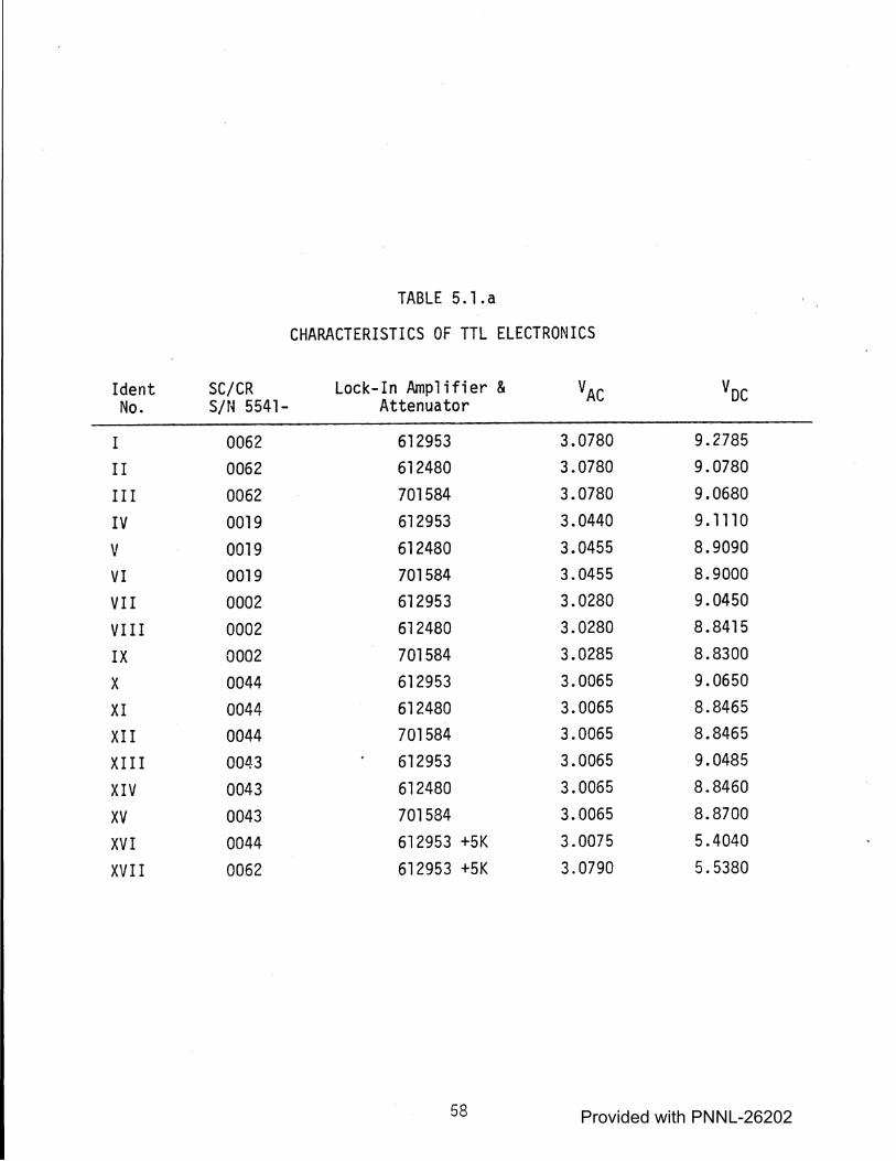
TABLE 5. l.a

CHARACTERISTICS OF TTL ELECTRONICS

!dent SC/CR Lock-In Amplifier & VAC Voe No. S/N 5541- Attenuator

I 0062 612953 3.0780 9.2.785

II 0062 612480 3.0780 9.0780

II I 0062 701584 3.0780 9.0680

IV 0019 612953 3.0440 9.1110

V 0019 612480 3.0455 8.9090

VI 0019 701584 3.0455 8.9000

VII 0002 612953 3.0280 9.0450

VIII 0002 612480 3.0280 8.8415

IX 0002 701584 3.0285 8.8300

X 0044 612953 3.0065 9.0650

XI 0044 612480 3.0065 8.8465

XII 0044 701584 3.0065 8.8465

XIII 0043 612953 3.0065 9.0485

XIV 0043 612480 3.0065 8.8460

xv 0043 701584 3.0065 8.8700

XVI 0044 612953 +SK 3.0075 5.4040

XVII 0062 612953 +SK 3.0790 5.5380


TABLE 5.1.b

TABLE OF CALIBRATION RUNS VERSUS ELECTRONICS !DENT. NO.

S/N I.D. {1) I. D. {2)

052 XI XIV 064 I XIII 078 II XIV 081 XVI I 098 XVI xv 109 I xv 110 XIV 128 xv I 156 II XIV 158 xv I 164 xv I 172 XIII VII l 91 VII VII AOTA XVII XVII 201 VII VII


6.0 REFERENCES

l. Letter, J. W. Mitchell to W. M. Jacobi, "GPL-2 Instrument S/A Testing - Preliminary Report," W/FFTF 721426, March l, 19?2.

2. D. R. Pederson, et al., "Flowmeter Calibration Report - SLSF Flo\'Alleters, 11 ANL/RAS 76-16, April 1976.

3. V. DeVita, "Calibration Report for HEDL Eddy Current and PM Flowmeters - H-3-42621 and H-3-42670," LMEC TI-12-LME-009, October 1977.

4. Letter, T. T. Anderson to W. B. Klingler, "Field Installation and Op~rating Instructions for the FC/T Module," Argonne National Laboratory, March 10, 1977.

5. Standard ROT C-4-7, "Eddy Current Probe Type Flow Sensor for Liquid Metal Service".

6. Standard, ROT C-10-5, "Eddy Current Power Supply and Signal -Conditioning Electronics."

7. M. Hirayama, "Theoretical Model of an Eddy Current Flowsensor, 11

IEEE Transactions on Nuclear Science NS-24, 2021 October 1977.

8. L. E. Fort, Private Communication.

9. K. Ara, "A Differential Transformer with Temperature and Excitation Independent Output," IEEE Transactions on Nuclear Science, IM-21, 249,August 1972.

10. G. Hughes, "Electrical Conductivity Fluctuations in High Temperature Liquid Metals," Journal of Physics E: Scientific Instruments 5, 349, 1972 •

J. D. Mccann, "Fast Response Temperature Sensor for Use in Liquid Sodium, "Journal of Physics E: Scientific Instruments 9, 298, · 1975 .

B. J. Farrington and G. Hughes, "A Theoretical Analysis Applied to Electromagnetic Instruments Used in Liquid Sodium, 11 Central Electricity Generating Board, Berkeley, Report RD/B/N275l, ·1975 .

B. S. Farrington and G. Hughes, 11 Performance of an Electromagnetic Temperature Sensor in Liquid Sodium," Journal of British Nuclear Energy 16, 347, October 1977 .

60


APPENDIX A

This Appendix contains the specifications for the following ECFM Components:

• PAR Model 128A Lock-In Amplifier

• PAR Model 5204 Lock-In Analyzer

A-1 Provided with PNNL-26202

PAR MODEL 128A SPECIFICATIONS

SIGNAL CHANNEL

FREQUENCY RANGE.: 0.5 Hz - 100 KHz

SENSITIVITY: 1 µV to 250 mV rms full scale in a 1-2.5-10 sequence.

INTERNAL NOISE: Less than 10 nV/Hz1/ 2 at l KHz.

SYSTEM GAIN STABILITY: Less than O.l%/°C.

DETECTOR BIAS: Adjustable from Oto ±15 V by inserting divider resistors on internal preamplifier board.

SIGNAL CHANNEL: Single-ended or true differential, switch-selectable.

INPUT IMPEDANCE: 100 megohms in parallel with 20 pF.

COMMON MODE REJECTION: Better than 100 dB at l KHz.

MAXIMUM COMMON MODE VOLTAGE: 3 V pk-pk to 20 KHZ, -6 dB/Octave above.

MAXIMUM INPUT SIGNAL: 1000 times full scale up to a maximum of 1.8 V pk-pk before overload.

HI-PASS FILTER: A front panel switch sets the high pass characteristics to <0.5 Hz (MIN. position), 5 Hz or 50 Hz. These values can be easily changed in the field to suit the application.

LOW-PASS FILTER: A front panel switch sets the low pass characteristics to 100 Hz, 10 KHz or >100 KHz (MAX. position). These values can be easily changed in the field to suit the application.

TUNED SIGNAL CHANNEL OPTION (128A/98): Provides a switch-selectable choice of a flat response or of a tuned bandpass (or notch charactersitic) at a set frequency with a Q of 5. The frequency can be adjusted over a 3:1 frequency range by means of a potentiometer, accessible from the rear panel, and can be changed to any frequency within the range of approximately 0.5 Hz to 100 KHz by changing capacitors mounted on solderless component clips on the board.


REFERENCE CHANNEL

FREQUENCY RANGE: 0.5 Hz - 100 KHz. No range switching or tuning required.

MODES OF OPERATION: Fundamental (f) - the Model 128A locks onto any external reference signal of the proper input characteristic. Harmonic (2f) - in this mode, the 128A will respond at the second harmonic of the external reference frequency, maximum input frequency is 50 KHz.

INPUT REQUIRED: The reference channel will phase lock to virtually any external voltage waveform of at least 100 mV pk-pk amplitude and which crosses its mean only twice each cycle. The minimum pulse duration (for asymmetrical waveforms) is 100 ns. The front panel Reference Unlock lamp indicates the presence of a proper reference input. When using a sine wave reference, best phase accuracy is achieved at l V rms.

ACQUISITION TIME: The time required for the reference channel lock to a changed reference signal is typically 2 seconds/octave. Below 5 Hz the acquisition time increases to 10 seconds/octave.

PHASE ADJUSTMENT: A calibrated ten-turn potentiometer provides O - 100° phase shift. The phase shift accuracy is better than 0.2° over the entire frequency range. Resolution is 0.1°. A four-position quadrant switch provides 90° phase shift increments accurate to 0.2°.

PHASE-SENSITIVE DETECTOR

DYNAMIC RESERVE: Asynchronous signals with amplitudes corresponding to 1000 times full scale can be applied without overload. Dynamic reserve can be greatly increased by modification 128A/70, 128A/98, and proper setting of high pass, low pass controls.

A-3


FILTER TIME CONSTANTS: l ms to 100 seconds plus an External position and a Minimum time position (less than 1 ms). The external position allows capacitance to be added via a rear panel connector to obtain any desired time constant. A de Pre-Filter switch is provided which inserts an additional 0.1 or 1 second time constant filter. When used in conjunction with any of the standard time constant settings, it provides a 12 dB/octave rolloff rate.

DC OUTPUT ZERO STABILITY: Better than 0.1%/°C, 0.1%/24 hours at constant temperature.

OUTPUT VOLTAGE: ±1 V full scale.

ZERO OFFSET: Calibrated ten-turn potentiometer allows up to ±lOx full scale signal to be suppressed.

OUTPUTS

METER READOUT: Zero-center taut-band meter to monitor de output.

RECORDER: ±1 V full scale at both a front panel BNC connector and a rear panel double banana jack for driving a recorder.

GENERAL

OVERLOAD: A front panel lamp indicates overload at all critical points in the instrument.

AMBIENT TEMPERATURE RANGE: The unit can be operated at temperatures ranging from 15°C to 45°C.

AUXILIARY POWER OUTPUT: Regulated± 15 Vat 20 mA available at a rear panel connector.

A-4


POWER REQUIREMENTS: 100-130 or 200-260 V ac; 50-60 Hz; 12 watts. Unit can also be powered from batteries by supplying ±20 to 30 V de to a rear panel connector. Batteries must be able to supply at least 250 mA.

SIZE: 17-3/411 w X 3-1/2 11 H X 1411 D (45 cm w X 9 cm H X 36 cm D).

WEIGHT: 14 lbs (6.4 kg).


PAR MODEL 5204 SPECIFICATIONS

SIGNAL CHANNEL

FREQUENCY: 0.5 Hz - 100 KHz

SENSITIVITY: 8 full-scale ranges from 100 microvolts to 250 millivolts in a 1-2.5-10 sequence. Three output expansion ranges of Xl, XlO and XlOO increase the overall sensitivity to 1 µV full scale.

INPUT: Single-ended or differential input, floating or grounded.

INPUT IMPEDANCE: 100 megohms shunted by 25 picofarads.

COMMON MODE REJECTION: Better than 100 dB at l KHz.

MAXIMUM COMMON MODE VOLTAGE: 3 V pk-pk to 20 KHZ -6 dB/octave. above 20 KHz.

MAXIMUM INPUT SIGNAL: 650 millivolts rms sine wave before overload (1.8 V pk-pk).

DETECTOR BIAS: Adjustable from Oto ±15 volts by inserting bias resistors on the internal preamplifier board.

HI PASS FILTER: A front panel switch sets high pass characteristics to <0.5 Hz (both sw~tches out), 5 Hz, or 50 Hz. These values can be changed in the field to suit the application.


LO PASS FILTER: A front panel switch sets low pass filter characteristics to 100 Hz, 10 kHz, or max (greater than 100 kHz). These values can be changed in the fieM to suit the application.

INTERNAL NOISE: Less than 10 nV/Hz112 at l kHz (see noise figure contour}.

SYSTEM GAIN STABTLITY: Setter than 0.1%/°C.

REFERENCE CHANNEL

FREQUENCY RANGE: 0.5 Hz to 100 kHz. no range switching or tuning required.

MODES OF OPERATION:

Fundamental (f): The reference channel locks onto any external reference signal having the proper reference characteristics (see below).

Harmonic (2f): The reference channel locks onto the proper external reference signal and responds to the second harmonic of the external reference.

INPUT REQUIRED: The reference channel phase locks to virtually any external voltage waveform having amplitude excursions of at least 50 millivolts on each· side of the mean crossing the mean only twice each cycle. Minimum pulse duration (for an asymnetrical wavefonn) is 5 microseconds. The front panel reference unlock lamp indicates the absence of a proper reference input. When using a sine wave reference, the best phase accuracy is achieved at 1 volt rms.

PHASE ADJUSTMENT: A calibrated ten-turn potentiometer provides 0-100 degree phase shift. The accuracy is within 0.2 degree and the resolution is 0.1 degree. A four-position quadrant switch provides 90 degree phase shift increments accuraate to 0.1 degree.

PHASE NOISE: Less than 0.1 degree (at l kHz; 0.1 sec, 12 dB/octave}.

ACQUISITION TIME:

0.5 Hz to 50 Hz - 15 sec (typical} 50 Hz to 100 kHz - 2 sec (typical}


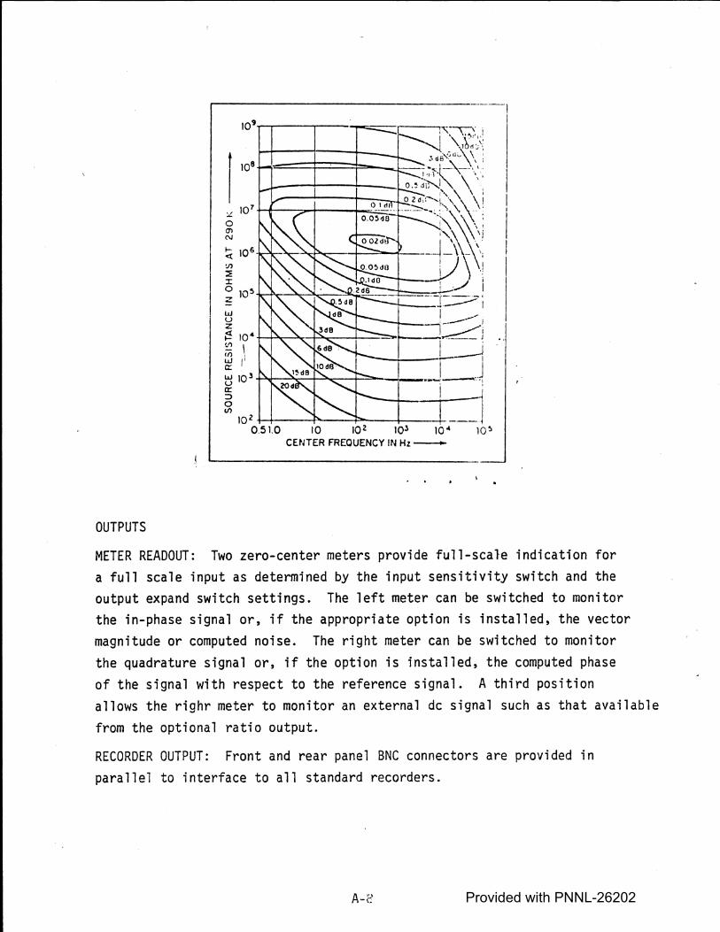
OUTPUTS

I ,a· :.! 10 7 t-11-~-t----l-=:::;;;.;:::::::J 0 (71 N

~ 106 -l,,,---'!,....,.,..--:,.,..p,.,.----1---=~-1

(/)

~ :I::

o 10'-i.,-i~~~-~~ z w u z ~ 10' ~~~_µ....,,__+--==-+--___; ~ l <fl I ~I ~ 10 3 ~'---":--+~-+-=--~a:: ::> 0 Ill

10 2 -4-+--_p..-__:~---+----l-Q5L0 10 ~z 10" 10'

CENTER FREQUENCY IN Hz -

--1 I

METER READOUT: Two zero-center meters provide full-scale indication for a full scale input as determined by the input sensitivity switch and the output expand switch settings. The left meter can be switched to monitor the in-phase signal or, if the appropriate option is installed, the vector magnitude or computed noise. The right meter can be switched to monitor the quadrature signal or, if the option is installed, the computed phase of the signal with respect to the reference signal. A third position allows the righr meter to monitor an external de signal such as that available from the optional ratio output.

RECORDER OUTPUT: Front and rear panel BNC connectors are provided in parallel to interface to all standard recorders.


OUTPUT VOLTAGE: l volt through 600 ohms.

METER SENSITIVITY (External Mode): l volt full scale. (100 µA meter movement through 10 kilohms.)

GENERAL

AMBIENT TEMPERATURE RANGE: Units can be operated at temperatures ranging from 15°C to 45°C.

AUXILIARY POWER OUTPUT: Regulated ±15 volts at 20 mA available at rear pa_ne l connector.

POWER REQUIREMENTS: 100 to 130 or 200 to 260 volts ac; 50-60 Hz; 35 watts. Units can also be powered from batteries by supplying ±24 V to± 30 V and +8 V de to a rear panel connector. Batteries must be able to supply at least 1 A.

SIZE: 17-1/2 11 w X 5-1/2" H X 19-l/211 D (.44.5 cm w X 13.9 cm H X 49.5 cm D).

WEIGHT: 25 lbs (11.4 kg).


APPENDIX B

This appendix provides a detailed calculation of the behavior of the induced EMFs in an ECFM made of three single loop coils. This simplification does not affect the applicability -of the qualitative results but does invalidate them for quantitative purposes.

Maxwell's field equations for the general case in which the medium .....

is moving with a velocity, V, are: .4

..... ...1. ...... ..... ..1. .... aD V x H = J + a (E + V + B) + ~ aT

~ ... ..I.

V X E = aB/ aT

.. ..J.

V • B = 0

( B. l)

(B.2)

(B.3)

(B.4)

...I. -4 where the only addition caused by the moving medium is the oV x B term in Equation (B.l).

...I. -J.

The divergence of B vanishes so, without loss of generality, B can be expressed in terms of a vector potential A,

~ ....I. ...l.

B = V X A (B.5)

Where A is not unique since it can be replaced by any vector function which differs from it by the gradient of some scalar function. This ambiguity does not reflect itself in the final answer and so is not considered.

Making use of Equations (B.l) - (B.5) along with the relation of D to E and B to H,

.-l. -I,

D = e: E, ...... -I,

B = µ H,

D 1

(B.6)

(B. 7)


which are valid in an isotropic, homogeneous medium. The following differential equation for A may be written when the driving current is sinusoidal;

~ .... .... .... 2 ... ...l. • a'A ~ ..-1. .!-.. V (V • A) - V A = µ J - µ (cr + 1 w e:) af + µ a V x (v + AJ (B.8)

which simplifies for the case in which Vis parallel to the Z-axis of the coil, since the current and vector potential are in thee direction. Hence, one can write,

-Jo /\

V = V Z

-', /\. A = A e

J= J 1-

(B.9)

(B.10)

{B.11)

where the caret denotes a unit vector and Equation (B.8), expressed in cylindrical coordinates becomes,

1 .a ( r ;~ l + a: 2A ',J:A - ar ;-i-2 - µ cr V a'z r

= cl + i 2 µ e:) A - µ J. {B. 11) r2

wµcr-w

The assumption of a single loop coil of radius a at Z = Z0 leads to,

(B.12)

This choice means that the solution for A is the Green function and can be used to create the general solution. Throughout, the assumption of invariance with respect to s has been tacitly assumed. Define A as the product of two functions,

~ A (r1 Z} = </> (r) $ (Z). (B.13)


The resulting equations for cf> and 1jJ can be obtai.ned by inserting Equation {8.13) in Equation {8.11).

=

1 cf> (r) r

1 - Tizl

lQ. [r 9_(r}] dr d r

[ d2 p(z) d z2

- ~1 - W µ {i O - WE) r2

V d 1J) (z)] µ 0 dz

o { r - a ) o (.z - z0 )

4{.z) (r)

(8.14)

In order to solve Equation (8.14), it is necessary to consider the solution for r >a. (.outside at the coil) as well as for z > z0 and z < z0 • For these cases, the two components can be separated and written as,

- µ a V ti= CijJ d z

l sL (r .Q_j) - J...2 = [ C + w µ (i a - w E}] cf> r dr dr r

(8.15)

(B. 16)

Because these are second order differential equations each possesses two solutions. The choice of solution is dictated by the boundary conditions. The solution of Equation (B. 16) is a linear combination of first-order modified Bessel functions, however only K1 survives because I1 is irregular at infinity. Equation (8.15) is solved by making the ansatz that

(8.17)

which results in

M2 - i aµ v M + C = 0 (8.18)

Choose C to simplify Equation (8.18),

C = (a2 + i aµ v a) (8.19)

B-3 Provided with PNNL-26202

which results in one solution, M = -a. The second solution is obtained from,

M- a - i er µ v = 0 ( B. 20)

Again applying the appropriate boundary conditions, 1/J becomes

$ (z) = 1/J e ia (z-zo) z < Zo (B.21) 0

(B.22) z > z

0

This two solution match at z = z0 as they should both remain finite in their respective regimes and the jump in the first derivative at z = z0

is erµ v w0 as it should be.

The choice of C given by Equation (.B.19), results in a solution for 1/J of,

(B.22)

where

a' is given by,

a' ~ ~ 2 + µ (i er Va+~ (i er - w €)) (B.23)

The final solution is obtained by integrating over the arbitrary parameter er,

(B.24)

aµv (z z) J"" K1 (a'.r) e-ia. (z-zo) d a z< z0 (B.25) A (r,z} = A0 e - o -""

B-4 Provided with PNNL-26202

Where A0 is an arbitrary normalization for A.

The voltage induced in the secondary coils is given by,

V =f E • ds = 2 ir b E6 = -2 ,r b a.A = -2 ir biwa .-at

where bis the radius of the secondary loops (b > a). Thus the EMF in the loop which·is upstream of the primary (z = z1) is given by,

(8.26)

J_: K, (a.' r) e -io (z1 - zo) ( B. 27) I

-Where A is a new normalization. The downstream loop (z = z2) sees an EMF of,

(B.28)

When crµv (z1 z0 ) is not large and when z1 z0 = z0 - z2. These two potentials can be related approximately by,

{8.29)

Hence, in the limit that cr andµ are constant and the expansion is valid, the difference of Vus and Vds is proportional to the sodium velocity, v,

(8.30)

Fluctuations in Vds' cr, µ and nonlinearities in Vus can lead to significant temperature dependent effects. (Vds is not independent of V since it appears in a. 1.) Self-compensating flowmeters use the difference and the sum to eliminate Vds" Thus they measure R,defined as the difference of the two potentials over the sum,which reduces to,

{ B. 31)

8-5 Provided with PNNL-26202

under the assumption of crµv (z1 - z0 ) being small. This self-compensated flowmeter sees a more linear reiationship between Rand flow.

In order to avoid the approximation of a small argument for the exponential, it is possible to examine the natural logarithm of the ratio

of vds to vus'

(8.32)

Pure temperature variations affect a andµ. Because of these effects, one can see that variations in crµv and in a 1 (see Equation (8.23) will have much less effect on Equations (8.31) and (8.32) than on Equation (8.30).

8-6 Provided with PNNL-26202

APPENDIX C

This appendix consists of the relevant procedures and standards for the PSD electronics:

• Setup and calibration procedure for the PAR Model 128A and 5204 Lock-In Amplifiers.

ECFM Lock-In Amplifier System Attenuator Design.

Field Calibration and Setup Procedure for the ECFM - Phase Sensitive Detectors.

C-1 Provided with PNNL-26202

SET.UP AND CALIBRATION PROCEDURE FOR THE PAR MODEL 128A AND 5204 LOCK-IN AMPLIFIERS

J. L. Stri riger November 21, 1978

I. GENERAL

These procedures cover the modifications, operational checks, and calibration for the PAR Models l28A/98 and the.5204/98 Lock-In Amplifiers. In all cases the amplifiers are new "just received".equipment whose proper operation and specific function calibration must be performed before the equipment is installed at FFTF.

II. EQUIPMENT MODIFICATION

A. Modifications for both 128A and 5204

B.

l. Install the rack mounting brackets on all instruments using the OZ-5204-35 kit on the· 5204 and brackets supplied by J. L. Stringer for the l28A's.

2. Install any hardware required to support the rear of the instrument cabinet required for mounting in the FFTF cabinets.

3. Remove the rubber feet from the bottom of all instrument chassis.

For only the 128A

Install a BNC connector in one of the rear chassis holes (selection TBD by J. L. Stringer) and connect it in para 11 el with the OUT connector on the front panel.

c. For only the 5204

Install a locking collet on the "Tuned Amplifier" frequency selecting patentiometer shaft {rear panel). Lock- collet will be supplied by J. L. Stringer.


III. INITIAL OPERATION CHECK

Both 5204 and 128A model.lock-in amplifiers were purchased with only t~e "TUNED AMPLIFIER OPTION" no other options are ins ta 11 ed.

A. For the 128A

Perform the instrumentation of the Section II initial checks section of the Operation and Maintenance Manual {OMM) with the following selections:

Paragraph 3.3 (3) Set tracking rate switch to FAST.

3.3 {4) lkHz was the ordered frequency.

3.3 (5) Skip Option not installed.

3.3 (8) These units were to have their gaih trimmed at the factory for a full scale indication on the 25 mV range, thus, the error may be {1% to 2%) larger than expected by this instruction.

8. For the 5204

Perform the instructions of Section III of the OMM "Initial Checks" with the following selections:

0 Perform only the paragraph 3.3 and 3.4 instructions.

0 Only the Tuned Amplifier option is installed.

·Iv. CALIBRATION

The calibration of the· two lock-in amplifier models shall be performed only after the Initial Operation checks of the Section III have been completed and shall be performed in the sequence listed in this section.

1. Test Equipment

(a) H/P model 6508 Sinewave Oscillator or equivalent with an adjustable amplitude and frequency with a 50 ohm output impedance.

(b) SO ohm or 75 ohm switch selected attenuator which can prov~de attenuation down to a ldb resolution.


-.1-

(c) Digital voltmeter such as a Fluke model 3200A or equivalent.

(d) Two BNC shorting plugs.

(e) Interconnecting cables.

(f) Frequency counter with an accuracy at 1 kHz to +0.5 Hz or better.

(g) General purpose oscilloscope.

2. Preliminary Steps

(a) Remove the top cover, which is secued by four screws, two on each side.

(b) Check and, if necessary, adjust the mechanical zero of the panel meters. Then plug in the Model 128A or 5204 turn on the power and allow a fifteen minute wann up minimum.

{c) Connect the BNC shorting plugs to both inputs.

3. Procedure for the 128A

Some of the instructions in this procedure will refer to the OMM for the 128A amplifier.

3.1 Power Supply Check·

On the power supply board, check for: (a) +15.SV +O.lV at the positive end of capacitor C309, (b) -15.SV +0.2V at the negative end of capacitor C310, and (c) +SV +0.2V at the positive end of capcitor C312. If these voltages are not .within the allowed variation notify J. L. Stringer (2-3418) before continuing.

Reference the OMM Section 6.4 and schematic on page VII-11.


-4-

3.2 Amplifier Control Settings:

Input Selector Switcb.: ·A Sensitivity: 25 mV Lo Pass Switch: 10 kHz Hi Pass Switch: 50 kHz Phase

Switch: 270° Dial: 90° (9:00)

Reference Mode Switch: f (fund.) Time Constant: O.~ sec. DC Prefilter: OUT Zero Offset

Switch: OFF (center position) Dial: 0.00 (fully counter clockwise)

Fast/Slow Switches (located on Ref. board): FAST

i

3.3 Test Configuration (See Figure 1).

3.3.l Connect the test system together as shown in Figure 1 except that one digital voltmeter (DVM) can be used for all measurement: Connection points should be provided in the test set up to allow quick connection of the DVM from point-to-point (BNC connectors)

3.3.2 Set the oscillator to l kHz+ 0.5 Hz with a nominal amplitude of 0.5 Vac Rms. (should always be within +5%).

3.3.3 Set the attenuator output to give 25 mVac:. 0.2% (requires approximately 26 db of attenuation) indication on the digital voltmeter.

3.4 Set Up the Tuned Amplifier and Lock-In Amplifier Gain.

• 3.4.1 Tuned Amplifier Switch Settings (Amplifier Board)

{a) Selecti~e/Flat Switch: {b) Notch/3andpass Switch:

Selective Notch ·

..... ... Provided with PNNL-26202

.....

Refer to OMM page IV-13, Figure IV-14~

3.4.2 Connect the oscilloscope to the Sig. Mon. BNC connector on the rear panel and set the oscilloscope to view a steady 1 kHz wavefonn~

3.4.3 Alternately adjust the tuned amplifier Freq. Adj. potentiometer (rear panel hole) and the NULL potentiometer (side wall hole) to obtain a minimum amplitude signal on the oscilloscope. These controls interact so several iterations will be necessary to obtain the best minimum.

NOTE: These controls should have been preset by the vendor for 1· kHz.

3.4.4 Set the Notch/Bandpass switch to Bandpass.

3.4.5 Adjust the Phase Dial (and Phase Switch if required) for peak (maximum) output voltage (Vdc) on the panel meter and Digital Voltmeter.

3.4.6 Adjust the Model 128A GAIN CAL. trim poteniometer, Rl43, for exactly +l.000 Vdc:. 0.0001 Vdc on the Digital Voltmeter. Refer to OMM page V~2, Figure V-1 for the location of Rl43.

3.5 Sensitivity Range Calibration

.. .This step determines the gajn sensitivities of the adjacent attenuator .'~ . ·.,:;. >·:.~-nnges· t250 mV, 100 mV, 10 mV and 2.5 mV).

. ,, '

3.5.l Set the Sensitivity Switch to the 250 mV position. -.. _··

3.5.2 Set the attenuator for a nominal 6 db of attenuation and : · .. ~djust the oscillator amplitude to give a reading of 250

rnV + 0.05 mV at the attenuator output.


-6-

3.5.3 Read the Model 128A output (Vdc) on the Digital Voltmeter and _record this reading versus the input voltage. The output voltage should be 1.00 Vdc + 0.02 Vdc. If not call to the attention of J. L. Stringer 2-3418.

3.5.4 Set the attenuator for a nominal 14 db of attenuation and adjust the oscillator amplitude to give a reading of 100 mV + 0. 05 mV.

3.5.5 Set the amplifier sensitivity to 100 mV and record the 128A Output voltage reading on the Digital Voltmeter versus the input voltage. Voltage should be 1.00 Vdc + 0.02 Vdc.

3.5.6 Repeat steps 3.5.4 and 3.5.5 for the following sensitivity switch settings and inputs.

Sensitivity 10 mV

2.5 mV

Input 10 mV + 0. 5 mV

2.5 mV + 0.5 mV

3.5.7 Return the Sensitivity switch to 25 mV.

Attenuator 34 db 46 db

This completes the calibration of the 128A Lock-In Amplifier.

4.0 Procedure for the 5204

Some of the instruction in this procedure will refer to the OMM for the 5204 amplifier.

4.1 Power Supply Check (DO NOT ADJUST)

In the OMM on Page VII-15 the circuit diagram 11092 and circuit board layout are shown for the power supply boards. Refer to these diagrams for the measurement locations.

4.1.1 Connect a Digital Voltmeter (DVM) across diode CR306 and verify a reading of+ 15.00 Vdc + 0.04 Vdc.


-7-

4.1.2 Connect the DVM across diode CR307 and verify a reading of - 15.00 Vdc + 0.04 Vdc.

4. 1 . 3 C_onnect the DVM across capacitor C304 and· verify + 5. O Vdc + 0.2 Vdc.

NOTE: If any of the voltages fall outside the limits call J. L. Stringer (2-3418) for further Instruction and stop the calibration.

4.2 Amplifier Control Settings

4.2.1 Front Panel:

Mode: Notch Float/Ground: Float A/A-B: A

Sensitivity: 25 mV Hi~h Pass: 50 Hz

Low Pass: 10 kHz

Phase (Reference) Push Button Depressed: 270° Dial: 90° (9:00) f/2f: f

EXT /I NT: EXT

In-Phase Zero Offset Dial: Fully CCW Zero Offset PB: OFF (Both released) DC Prefilter PB: 0.1 Sec (depressed) Output Expand PB: X1 (depressed) Time Constant: 0.3 sec.

Meter PB In-Phase: depressed Quadrature: depressed


·Quadrature Zero Offset dial: Fully CCW.

· · Zero Offset PB: Off (both rel eased) DC Prefilter PB: 0.1 sec (depressed) Output Expand PB: Xl (depressed) Time Constant: o.j sec.

4.2.2 Rear Panel

Tuned Amplifier Range Switch: l kHz Multiplier: Near 1 (subject to final tuning)

4.3 Test Configuration (See Figure 1) '

4.3.1 Rep~at Steps 3.3.1 through 3.3.3

4.3.l Connect a DVM to the In Phase (I) Output BNC.

4.4 Set up the Tuned Amplifier and Lock-In Amplifier Gain

4.4.1 Adjust the Tuned Amplifier Range. and Multiplier controls set up in 4.2.2 to achieve a decreased level on the In Phase meter and DVM.

4.4.2 Alternately adjust the Multiplier and Notch Depth controls to get the smallest indication on the In Phase meter. Increase the measurement sensitivity by first operating the output expansion PB to XlO then to XlOO and finally move the Sensitivity switch to 10 mV, 2.5 mV, etc., until no further decrease can be achieved or the overload light becomes illuminated.

4.4.3 Return the Sensitivity switch to 25 mV and the Output Expand PB to Xl (depressed).

4.4.4 Depress the Bandpass pushbutton the In Phase(!) ~eter should indicate near full scale and the Quadrature (Q) meter should indicate near ze~o.


... ·_ ~ .

4.4.5 Move the phase dial to get the best zero on the Q meter and a maximum reading on the I meter a·nd DVM.

NOTE: . Use the Q meter Output Expand ranges of XlO and XlOO to complete the final adjustment, then return the Output ~xpand to Xl.

4.4.6 Referring to pages VII-12 and VII-13 for the schematic and parts location on the Signal Amplifier Board, adjust Rl43 Gain Adj. potentiometer to give an output on the I meter of l.' 000 Vdc + . 0001 Vdc.

4.4.7 Depress the 180° phase pushbutton and change the DVM to the Q meter output. Verify that the Q output voltage is 1.000 Vdc + 0.0005 Vdc. . -

. 4.4.8· Return the DVM to the I meter output and depress the 270°

Phase pushbutton.

This completes setting up the gain of the 5204 for the 25 mV sensitivity range to an accuracy.! 0.2%.

4.5 Sensitivity Range Calibration

This step determines the relative gain sensitivities of the adjacent attenuator ranges (250 mV, 100 mV, 10 mV and 2.5 mV).

4.5.1 Set the Sensitivity switch to the 250 mV position.

4.5.2 Set the attenuator f6r a nominal 6 db of attenuation and ~djust (trim) the oscillator amplitude to give a reading of 250 mV + 0.05 mV at the attenuator output.

4.5.3 Read the I meter output (Vdc) on the DVM and record the readi~g versus the input voltage. The output voltage should be

. ·witnin 1.000 Vdc + 0.020 Vdc.


4.5.4 Set the attenuator for a nominal 14 db of attenuation and trim the oscillator ~mpli-tude to give a reading of 100 mV + 0.05 mV ..

4.5.5 Set the 5204 sensitivity switch.to 100 mV and read the I meter output (Vdc) on the DVM and record this reading versus the input voltage. This voltage should be within the range of l.000 Vdc + 0.020 Vdi:.

4.5.6 Repeat steps 4.5.4 and 4.5.5 for the following sensitivity switch settings and inputs.

Sensitivity 10 mV

2.5 mV

Input 10 mV + • 05 mV

2.5 mV-+ .05 mV

4.5.7 Return t~e Sensitivity switch to 25 mV.

Attenuator 34 db 46 db

This completes the calibration of _the 5204 Lock-In Amplifier.


FREQUENCY COUNTER

ACCURACY: 1000. Hz ± 0. 1 Hz

SINEWAVE OSCILLATOR

Zo = 50n o. 5 Vac ± 5% O. lk Hz + 0. 5 Hz

DIGITAL VOLTMETER ACCURACY - @25 mV,

lk Hz -± 0. 2%

DIGITAL VOLTMETER VDC ACCURACY

1. 000 Vds. ± 0. 01 % -

DIGITAL VOLTMETER

- ACCURACY: ± 0. 5% AT 1 k Hz

AMPL. SENS. RANGE

0.250 0.100 0.025 0.010

STEP 0.0025 ATIENUAT,OR

o SIG. INPUT REF. INPUT PAR

128A OR 5204

LOCf ~:N AMPLIFIER Q• (~:v) I I

- - - - _____ ..J ... - .

Fl GURE 1 HEDL 7904-152.1

ATTEN. SETTING (db)

6 14 26 34 46


I. DESIGN DECISIONS:

SYSTEM ATTENUATOR ECFM LOCK-IN AMPLIFIER DESIGN

J. L. Stringer December 4~ 1978

1. Since the new PAR lock-in amplifiers have a 25 mV sensitivity ranga rather than 20 mV and a 1.000 Vdc output rather than 10.00 Vdc, it was decided to design the atfenuator ~o matth the 25 mV input signal, but allow the factor of 10 reduction in the output (no cho1ce}.

2. The gain errors from the original calibration of the ECFM's for the lockin· amplifier/attenuator combinations for each chanel is+ 1.1%, (-) .79%. The gain error between channels (Attenuator/Amplifier No. l; Attenuator/ Amplifier No. 2) is(+) 1.3%, (-} .78%.

3. The tolerance of the lOk ohm buffer resis.tor in the FFTF-ECFM-SC/CR module is+ 5%.

4. From these data the total variation which must be accomodated by the attenuator is:

+ 5%, + 1.3%, + 1.1%

Linearly combining these variations gives

+ 7.4%

as the variation range for the adjustment, and is the design goal.

5. A variation of! 10% was:;·:~ to make the initial design choices.

6. The fi~al design choices ~~~e made for the components available from Rockwe 11 ·Stores.


II.

7. A circuit design was chosen to make the attenuator input and output impedances nearly contant near the values used for the calibration attenuators .. ,

8. The circuit ground will be carri~d separate from chassis ground to be consistant with the grounding practices in use at FFTF and the floating input on the PAR amplifiers.·

CIRCUIT DESIGN (Nominal Values)

I R1 i

{------,,5k/\.__.__~> R2 R3

I soo 1 oo f I I I I I pl Trim R4 I I 2k 0 49.9

10% Adj. I I I I I J-- ________ .J.. ~ Chassis Ground -

All resistor values in ohm All resistors are 1/4 w, 1%, metal film Potentionmeter is cermet, 20 turn

The nominal setting of P1 to give ·an output of 0.0250 volts for a 1.000 V input is P1,0 = 382 ohms.

FIGURE 1

... ,The-.:~uation. for the;_11omina 1 "'.attenuator is:


-3-

Evaluating with the nominal values gives

and

and

then

Rs= R3 + R4 = 100 + 50 = 150 n

R2 + P1 = 500 + 382 = 882 n

Rs(R2 +Pl)= 150(500 + 382) = Rs+ R2 + pl 150 + 500 + 382

Vo _ _ 128.2 _ Vin - n - 5000 + 128.2- ·0250

128.2 n

This result can be interpreted to mean, when 1 volt is applied to the attenuator input .0250 volts is applied to the amplifier input.

The nominal input impedance of the attenuator is

5000 + 128.2 = 5.1282k ohms+ 1%

The ECFM calibration attenuator nominal input impedance was 5.10k ohms + 1%.

The nominal output impedance of this attenuator design is

(128.2)(5000) = 125 ohms+ 1% 128.2 + 5000 -

The nominal ~utput of the ECFM c~libration attenuator was

(lOO)(SOOO) = 98.0 ohms+ 1%. 100 + 5000

CIRCUIT VARIATION RANGE

Note the following circuit components and their tolerances.


R1 = 5000 n, :!:_ l %

R2 = 500 n. + 1 % .

R3 = 100 n, :!:. 1%

R4 = 50 n, + 1%

--,-

P1 = 2000 n + 10% and~ 2 n residual resistance

R3 + R4 = 150 n, + 1%

The attenuator circuit can be~redrawn as

•

Vin

j

5k 1%

Variation Analysis:

R. 2

500 1%

. FIGURE .2

pl 2k

10%

Rs 150

1%

1 Vo

The various circuit element combinations will be calculated for the maximum and minimum v~riation around the nominal attenuator value of 0.0250.

The minimum output voltage of the R1 , Rs circuit branch ocurrs when

Rs= 148.5 (- 1%) ohm

R~ ~ 5050 (+ 1%) ohms

The maximum output voltage of the R1, Rs circuit branch ocurrs when

Rs= 151.5 (+ 1%) ohms

R1 = 4950 (- 1%) ohms. Provided with PNNL-26202

-5-

The R2, P1 circuit branch just modifies the Rs circuit value, thus, when the R2, P1 circuit has its maximum value the parallel combination of Rs and (R2 + P1l will have its maximum value, an~ when (R2 + P1) has its minimum value the paralle· combination of Rs and (R2 + P1) wilL have its minimum value.

Thus, only four cases need to be calculated. These are:

CASE I:

Rs= 148.5 n

R1 = 5050 n

R2 = 495 n

P1 = 1800 n

n(R1, Rs)= minimum

R2 + P1 = minimum (Adj. ~igh)

_.Rs (R2 +Pl)_ 148.5 {2295) _ 139_5 n RP - Rs+ R2 + P1 - 148.5 + 2295 -

Vo _ RP _ 139. Vin - R1 + RP - 139.5 + 5050

Minimum(+) variation%

.02688 - .02500 X lQQ = +7 52% .02500 •

CASE II:

Rs = 151. 5

R1 = 4950

R2 = 505

pl = 2200

· Rs (R2 + P1) RP= R + R + Pl ~

s 2

~(R1, R) = maximum . s R2 + P1 = maximum (Adj. High)

151.5 (505 + 2200) _ 151.5 + 505 + 2200 -. 143 ~5 a

Vo _ RP _ 143. 5 = Vin - R, + R ~ 4950 + 143.5 .02817

I p ,

Max(+) ·variation%

.02817 - .02500 .QZSOQ X 100 = + 12.7%


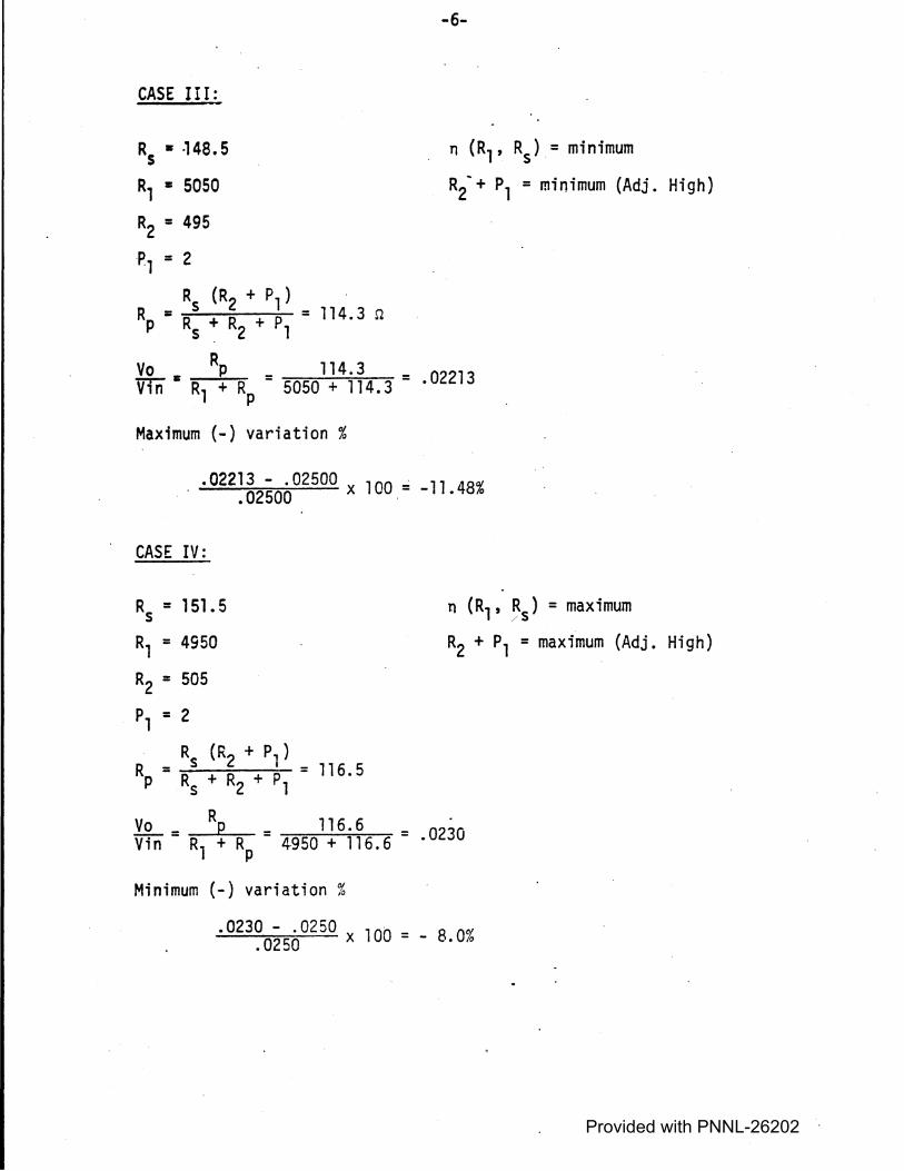
CASE III:

R5 • -148.5

R1 • 5050

R2 = 495

-P1 = 2

R {R2 + P1) · RP= Rs+ R + p = 114.3 n

s . 2 1

Vo • RP _ 114.3 _ Vfn R1 + RP - 5050 + 114.3 -

Maximum{-) variation%

-6-

n {R1, Rs)= minimum

R2'+ P1 = minimum (Adj. High)

.02213

.02213 - .02500 X lOO = -ll 48% . • 02500 •

CASE IV:

Rs = 151. 5

R1 = 4950

R2 = 505

pl= 2

. Rs (R2 + Pl) RP= R + R + p = 116.5

s 2 l

R Vo = p = 116. 6 = Vin R1 + RP 4950 + 116.6

Minimum(-) variation%

. n (R1, , 5 ) = maximum

R2 + P1 = maximum (Adj. High)

.0230

.0230 - .0250 X lOQ _ B Q% .0250 - - .


-7-

Thus, the minimum positive attenuation variation value is+ 7.52% while minimum negative attenuation variation value is - 8-•. 0%.

SUMMARY

The positive and negative adjustment limits with the component tolerance chosen bracket the expected+ 7.4% system variation and should provide the long term stability that is necessary for the system operation.

,'.)


GENERAL

FIELD CALIBRATION

AND SET UP PROCEDURE FOR THE ECFM - PHASE .SENSITIVE DETECTORS

J. L. Stringer December 13~ 1978

This procedure is focused on setting the PSD external attenuator to the TTL

calibration gain requirements for the specific ECFM sensor being calibrated, and to adjust the phase space position of the in-phase PSD component to coincide with the sensor's flow vector.

PROCEDURE

1.0 Preliminary

1.1 Equipment Required

a. Interconnecting cables and adapters.

b. FLUKE - DVM in the ECFM test section for Vac measurements.

c. Hand calculator SR-50, TI-30 or equivalent.

d. Portable DVM with resolution and accuracy to 1 mVdc on a 1-2 Vdc full scale range.

1.2 Equipment Warm Up

The equipment shdll have been turned on far 30 minutes following the last 2 to 3 minute duration without power prior to performing the procedural steps.

The attenuator calibration procedures shall be performed without power interruption.

1. 3 Assumptions

1.3.l This procedure assumes that the Model 1?8A's.and 5204(l) have completed the gain ca1ibratiolis in the Standards Laboratory( 2), have been installed in the appropriate ECFM cabinets at FFTF and( 3)


that the systems are interconnected per the connection diagram of Ftgure 1.

1.3.2 These procedures can be performed only following compilation and certification of FTRTA - ECFM - SC/CR module gain adjustment to a procedure equivalent to that of paragraph 5.4.1.4 (Gain Adjust) page 59 of OHM-092-00-002, Vol. l.

1.4 Initial Control Settings

a. Model 128A

Input Selector Switch: A Sensitivity: 25 millivolts Lo Pass Switch: 10 kHz Hi Pass Switch: 50 Hz Phase:

Switch: 270° Dial: goo (9:00)

Reference Model Switch: f (fundamental) Time Constant: 3.0 sec. DC Prefilter: Out Zero Offset:

Switch: Off (Center Position) Dial: 0.00 (full ccw)

b. Model 5204 Front Panel

Mode: Bandpass (PB depressed) Float/Ground: Float (PB depressed) A/A-B: A (PB depressed) Sensitivity: 25 mV High Pass: 50 Hz (PB depressed) Low Pass: 10 kHz (PB depressed) Phase (Reference)

PB: 270° (depressed) Dial: go 0 (9:00)


· Mode (reference)

In-Phase

2f/f: f (PB released) Ext/Int: Ext (PB depressed)

Zero Offset Dial: fully ccw Zero Offset PB: Off (both released) DC Prefilter PB: Off (both released) Output Expand PB: Xl (depressed) Time Constant: 3.0 sec.

In-Phase Meter In-Phase PB: Depressed

Quadrature Meter Quadrature PB: Depressed

Quadrature Zero Offset Dial: Full ccw Zero Offset PB: Off (both released) DC Prefilter PB: Off (both ·released) Output Expand PB: Xl (depressed) Time Constant: 3.0 seconds

Rear Panel

Tuned Amplifier Range Switch: lkHz

2.0 Calibrate the PSD Attenuator/Lock-In Amplifier

2. 1 Verify that the flowsensor is installed and connected to the correct SC/CR module position.

2.2 Verify that the PSD system is interconnected per Figure 1 and that power has been turned on for at least 30 minutes.

2.3 Verify that the ECFM-SC/CR module/flowsensor have been energized for at least 30 minutes, and has been calibrated to the requirements of paragraph 1.3.2.


2~4 Verify that the Lock-In Amplifier controls are setup per paragraph 1.4 for the appropriate lock-In module.

2.5 Verify that the REF UNLOCK light in the Reference Section of the Lock-In . Amplifier is not illuminated.

2.6 Connect the Test and Readout {T&R) cable between the Module Test Cable connector J204 on the Test/Cal Station and the Selected SC/CR module test connector.

2.7 With the T&R cable attached, remove the SC/CR module from its operating position and insert it fully into the Test Station test slot.

2.8 Set Test/Cal Station controls as follows:

Control/Switch

Unit Test Select SC/CR TEST SEL SC TEST FUNCTION AMPL CONTROL DMM

Position

SC/CR . AMPL SEC GAIN

400 (4.00 mV) 10 V-AC

2.9 Verify that the DMM reads+ 3.03 Vac (+ 1%) with the cable to J3 SC/CR disconnected. Record this reading 3. Vac.

2.10 Reconnect the cable to J3 (AMPL SEC) on the SC/CR module and note that the DMM reading drops to 1.02 Vdc ±. .07 Vdc.

2. 11 While monitoring the OUT DC voltage with portab!e DVM (2 Vdc max, 10C% overage of output) adjust the dial phase control and the course switch or pushbutton controls to achieve a maximum in-phase output voltage and/or a zero quadrature voltage.

NOTE: The quadrature output for the Model 5204 is read from the Q outp~t connector directly. For the Model 128A change the course phase dial by 90° leading or lagging and read the DVM output while adjusting the phase dial to get zero Vdc.


2.12 Return the Lock-In Amplifier course phase controls to display the maximum in-phase·signal. Record the final phase readings. Switch~~~ Dial~~~~

2. 13 ·Adjust the associated PSD attenuator section, adjust potentiometer to get a Vdc output from the Lock-In Amplifier determined in the following manner.

Multiply the voltage reading obtained in step 2.9 by the gain number associated with the ECFM probe being calibrated listed in the gain number column of Table I.

For example:

If the step 2.9 voltage is 3.04 and the Gain Number from Table I is 0.302 the Vdc output voltage will be:

3.04 X .302 = 0.918 Vdc

2. 14 When the Lock-In Amplifier reads the calculated output v9ltage stop the adjustment, remove the adjustment tool, and cover the adjustment hole with an appropriate label which includes the ECFM No., and SC/CR No., serial number of associated Lock-In Amplifier, and the final output voltage measured.

2. 15 Return the SC/CR module to its correct panel location and disconnect the T&R cable.

2. 16 This completes the PSD attenuator calibration for this channel.

2.17 Continue to repeat the procedure steps until eleven PSD attenuator sections are adjusted.

2. 18 Proceed to setting up the PSD detector in the direction of the flow vector section 3.0.


3.0 Lock-In Amplifier Phase Adjustment For Flow Measurement

3.1 Verify that the flowsensor is connected to the correct SC/CR module position, PSD attenuator and Lock-In Amplifier.

3.2 Verify that the PSD system is connected according to Figure 1.

3.3 Verify that power has been applied to both the SC/CR module and the Lock-In Amplifier for at least 30 minutes.

3.4 Verify that section 2.0 of this procedure has been completed for this PSD system.

3.5 Verify that the Lock-In Amplifier controls are set up per paragraph 1.4 for the appropriate Lock-In module.

3.6 Verify that the REF UNLOCK light in the reference section of the Lock-In Amplifier is not illuminated.

3.7 Set up the Switch/Pushbutton and dial phase settings determined in the TTL calibration for the ECFM selected. These settings are listed in Table I for the selected ECFM.

3.8 Set the reactor sodium flow past the ECFM's to zero (all pumps off).

3.9 Observe the in-phase (IP) and quadrature (QP) (+ 90°) signal magnitude and polarities, with the portable DVM, and adjust the phase switch and dial settings to get the magnitudes and polarities for IP and QP listed in Table I.

3. 10 Record these magnitudes and phase settings in Section I of Addendum I.

3.11 Repeat the procedure step 3.1 through 3.10 for all the Lock-In Amplifier systems being set up.

3.12 Increase the flow by operating bm or three (3 preferred) of the primary system pony motors.


.--------------------------------------- --

3.13 Without performing any adjustments on the phase of the Lock-In Amplifier, record the IP and QP -output voltages in Section I of Addendum I for the maximum fl ow .

. NOTE: This procedure may not be adequate for those flowsensors positioned over the reflector position. A procedure addition may result from the field measurements being made.

3.14 Following completing steps 3.7 through 3.13 for all amplifiers transfer the voltage values recorded in Section I of Addendum I to the 11, 12, q1, and q2 values of Addendum II according to the following:

11 = IP at 3 pony motor flow, 400°F.

ql = QP at 3 pony motor flow, 400°F.

12 = IP at zero flow, 400°F.

q2 = QP at zero flow, 400°F.

3. 15 Perform the calculations indicated on Addendum II to get the correct 3 pony motor flow value for the QP voltage setting. Also, graph the 11, 12, q1, and q2 values and graphically verify the calculated value.

3. 16 Record the QP calculated value in Section II Addendum I.

3. 17 Repeat steps 3.14 through 3. 16 for all the Lock-In Amplifier systems being set up.

3.18 While the three pony motor flow continues set the phase switch on the selected lock-in system to measure QP, and slowJy adjust the phase dial to get as near to the calculated QP value as possible over a 5 minute time period.

3. 19 Record the IP and QP voltage values in Section II of Addendum I.


3.20 Repeat steps. 3.18 and 3. 19 for all lock-in systems.

3.21 If possible lower the flow back to that used in step 3.9 and 3.10 and record the QP and IP output voltage in Section II of Addendum I as zero

· flow.

3.22 Repeat step 3.21 for all lock-in systems.

3.23 Resume 3 pony motor or selected flow.

3.24 Remove the DVM from the outputs.

3.25 Verify that the course phase switch is set to display the IP vector component on the meter and that the output connector is connected to the DOH and DS input.

3.26 This completes set up of the Lock-In Amplifier system after MIST operation.


ADDENDUM I LOCK-IN AMPLIFIER/ECFM SET UP

Date: Trial Run No.: ECFM No.: -------- ------ -------Reactor Position: __________ ECFM SC/CR No.: __________ _

DOH & OS Channel No.: _______ Lock-In Amp/Attn. No.: _____ ____,/...__ __

NA Temp.: °F, Name and Initial: --- ------------------Calibrator

Section I

Na Flow - 3 pony motors · - @400°F

Na Fl ow - near Zero @400°F

Section II

Na Flow= 3 pony motors @400°F

Na Flow= near Zero @400°F (Check Of QP)

IP = Vdc ( 0 + -------QP = Vdc ( 0 +

-IP= Vdc ( 0 + -------QP = Vdc ( 0 +

CALCULATED QP = Vdc -------

IP= Vdc ( 0 +

QP = Vdc ( 0 +

IP= Vdc ( 0 +

QP = Vdc ( 0 +

0)

0)

0)

0)

0)

0)


ADDENDUM II CALCULATE QP

Date: Trial Run No.: ECFM No.: --------- -------- -------

Reactor Position: __________ ECFM SC/CR No.: ___________ _

OOH & OS Channel No. Lock-In Amp/Attn. No.: / ---------- ___ _...;:..,___ __ _ Na Temp. : ___ °F, Name and Initial: ______ ._,........,...,,-,---,-----------

Calibrator

,, = ______ _

12 =-------

ql = -------

q2 = --------

C.a1culate: {Observe Algebraic Sign Laws)

=

-1 ,,

0 = tan = ql

0 = tan-l (ql -q2) = 1, 12

Cos (0 + 0)

'op = -----------

------·· -· -l • • -------- _______ ! __ .. ··-·· --- - •. -1---· - -------~----- --- ------·-·t ------- ---- -- :· -- ---- - __ _; --~ ~-~: -: ~-~~ :_1 :-_:_: ___ :~~ -~-~~~;~:~: :·:~ .. :~=~-~=~~=--~-~:.~--=-~~--.- .;.~~-:---~=-==--=~2---=~~=~~~~--~-~~~

_: :-:: : : : =-- ~~ ;:: :_=.::=-~: ::_:·~-:==-: ::-=::=:_:-.: =r=-: :.-~:---=-==--~i-=--~.::.-=·:-:--::~::...~=::---=:--:-:-.._-- __ -:: . - . -- . . ~ - - . -- . .

'• ' . -- .• t ..

---------------------------

' ... r . I


-----~

"

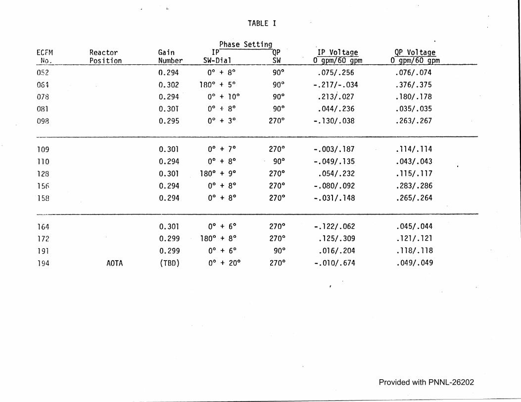
TABLE I

Phase Setting ECFM Reactor Gain IP QP IP Voltaqe QP Voltage

No. Posit ion Number SW-Dial SW 0 gpm/60 gpm 0 gpm/60 gpm 052 0.294 oo + ao goo .075/.256 .076/.074

06l 0.302 180° + 5° goo -.217/-.034 .376/.375 078 0.294 0° + 10° goo .213/.027 .180/ .178 081 0.30T oo + 30 goo .044/.236 . 035/. 035

098 0.295 oo + 30 270° -.130/.038 .263/.267

109 0.301 oo + 70 270° -.003/.187 . 114/. 114

110 0.294 ao + 30 goo - . 049/. 135 .043/.043

128 0.301 180° + 9° 270° .054/.232 . 115/. 117

156 0.294 ao + 80 270° -.080/.092 .283/.286

15B 0.294 oo + 80 270° -.031/.148 .265/.264

164 0.301 oo + 60 270° -.122/.062 .045/.044

172 0.299 180° + 8° 270° .125/.309 .121/.121

191 0.299 oo + 60 goo . 016/. 204 . 118/. 118

194 AOTA {TBD) 0° + 20° 270° -.010/.674 .049/.049


AMPL SEC

DRIVE CURRENT

J5

~

TYPICAL CHANNEL WI RE ROUTING

BNC CONNECTORS

COAXIAL(D CABLE

RG/58A/U0

[]

"

SC/CR TEST_....,.. _____ ...__......,;a

ATIEN #1

ADJ 0

IN OUT

ATIEN ATIEN ATIEN #2 #3 #4 ADJ ADJ ADJ 0 0 0

(Q)(Q) (Q)(Q) ©© BNC CONNECTORS

,~1 ADJ

' I '

-'~-

CONSTANT

co OFFSET OUT ~Q

FROM REAR --"""""'"- - - ~ PANEL OUT II 115 VAC CONNECTOR

f -..1 MODEL 5204

TO FFTF OVER

DOH & DS SYSTEMS

· HEDL 7904-152. 2 Provided with PNNL-26202

DOE/FFTFPO

Director (5) G. D. Bouchey T. L. King

HEDL

S. L. Addi ton T. A. Basmajian R. A. Bennett P. B. Bourne J. W. Connel l D. C. Corrigan E. R. Cramer A~ D. Danko L. V. Feigenbutz L. F. Fort W. M. Gajewski C. W. Hoth R. J. Jackson H~ G. Johnson w. L. Knecht W. J. McShane D. E. Mahagin W. T. Nutt (6) R. J. Robinson D. P. SchiveJy L. K. Severud E. M. Sheen D. E. Simpson D. D. Stepnewski J. L. Stringer (6) W. L. Thorne J. C. Tobin R. P. Warrick W. R. Wyckoff M. W. Young

DISTRIBUTION

W/8-18 W/A-59 W/B-43 W/8-118 W/0-56 W/C-3 W/8-48 W/D-18 W/C-6 W/0-56 W/B-82 W/E-32 W/E-32 W/8-43 W/0-66 W/8-12 W/A-59 W/8-18 W/B-86 W/8-48 W/C-99 W/A-56 ~1/C-BO W/C-75 W/A-56 W/A-ll W/8-33 W/D-56 W/D-56 W/B-106

Central Files (10) Publications and Services (2)

.. HEDL-TC-1344


eddy current flow measurements in the fftf

Documents