edc3 1.0 introduction - iowa state universityhome.engineering.iastate.edu/~jdm/ee553/edc3.pdf · to...
TRANSCRIPT

1
EDC3
1.0 Introduction
In the last set of notes (EDC2), we saw how
to use penalty factors in solving the EDC
problem with losses. In this set of notes, we
want to address two closely related issues.
What are, exactly, penalty factors?
How to obtain the penalty factors in
practice?
2.0 What are penalty factors?
Recall the definition:
Gi
GmGL
i
P
PPPL
),,(1
1
2 (1)
In order to gain intuitive insight into what is
a penalty factor, let’s replace the numerator
and denominator of the partial derivative in
(1) with the approximation of ΔPL/ΔPGi, so:

2
Gi
L
i
P
PL
1
1
(2)
Multiplying top and bottom by ΔPGi, we get:
LGi
Gii
PP
PL
(3)
What is ΔPGi? It is a small change in
generation. But that cannot be all, because if
you make a change in generation, then there
must be a change in injection at, at least, one
other bus. Let’s assume that a compensating
change is distributed throughout all other
load buses according to a fixed percentage
for each bus. By doing so, we are embracing
the so-called “conforming load” assumption,
which indicates that all loads change
proportionally.
Therefore ΔPGi=ΔPD. But this will also
cause a change in losses of ΔPL, which will
be offset by a compensating change in swing
bus generation ΔPG1. So,
3
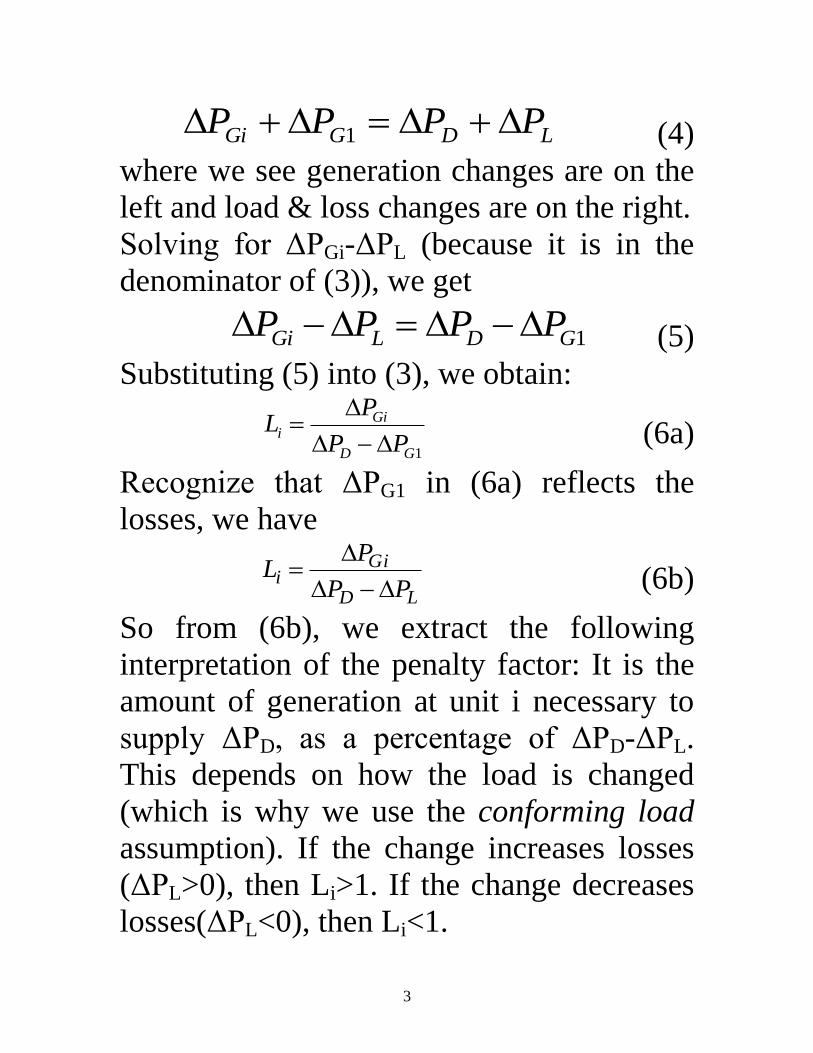
LDGGi PPPP 1 (4)
where we see generation changes are on the
left and load & loss changes are on the right.
Solving for ΔPGi-ΔPL (because it is in the
denominator of (3)), we get
1GDLGi PPPP (5)
Substituting (5) into (3), we obtain:
1GD
Gii
PP
PL
(6a)
Recognize that ΔPG1 in (6a) reflects the
losses, we have
LD
Gii
PP
PL
(6b)
So from (6b), we extract the following
interpretation of the penalty factor: It is the
amount of generation at unit i necessary to
supply ΔPD, as a percentage of ΔPD-ΔPL.
This depends on how the load is changed
(which is why we use the conforming load
assumption). If the change increases losses
(ΔPL>0), then Li>1. If the change decreases
losses(ΔPL<0), then Li<1.
4
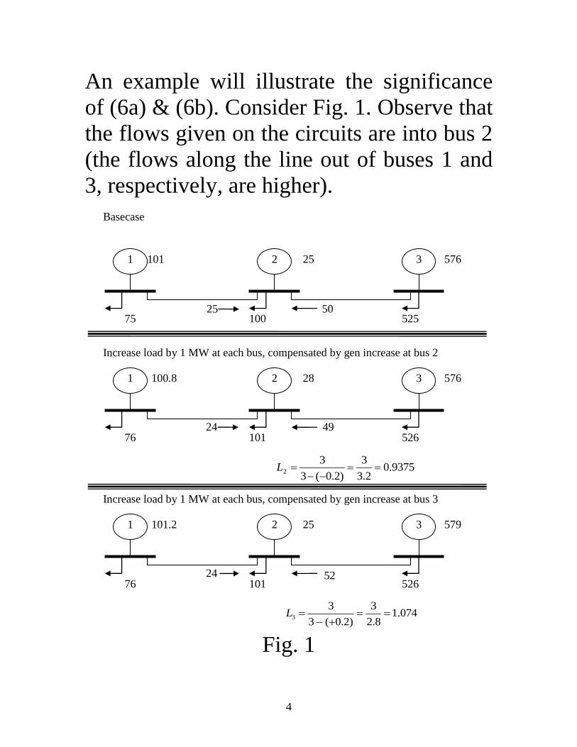
An example will illustrate the significance
of (6a) & (6b). Consider Fig. 1. Observe that
the flows given on the circuits are into bus 2
(the flows along the line out of buses 1 and
3, respectively, are higher).
75 100 525
101 25 576
25 50
Increase load by 1 MW at each bus, compensated by gen increase at bus 2
1 2 3
76 101 526
100.8 28 576
49
1 2 3
9375.02.3
3
)2.0(3
32
L
Basecase
Increase load by 1 MW at each bus, compensated by gen increase at bus 3
76 101 526
101.2 25 579
24 52
1 2 3
074.18.2
3
)2.0(3
33
L
24
Fig. 1

5
One observes that L2<1. This is because a
load change compensated by a gen change at
bus 2 decreases the losses as indicated by
the fact that the bus 1 generation decreased
by 0.2 MW.
On the other hand, L3>1. This is because a
load change compensated by a gen change at
bus 3 increases the losses as indicated by the
fact that the bus 1 generation increases by
0.2. MW.
Why does the bus 2 generation reduce losses
whereas the bus 3 generation increases
losses?
Answer: Because increasing bus 2 tends to
reduce line flows, whereas increasing bus 3
tends to increase line flows.
So we see that in general, generators on
the receiving end of flows will tend to have
lower penalty factors (below 1.0); generators
on the sending end of flows will tend to
have higher penalty factors (above 1.0).

6
Because transmission systems are in fact
relatively efficient, with reasonably small
losses in the circuits, the amount of
generation necessary to supply a load
change tends to be very close to that load
change. Therefore penalty factors tend to be
relatively close to 1.0.
A list of typical penalty factors for the
power system in Northern California is
illustrated in Fig. 2. Generators marked to
the right are units in the San Francisco Bay
Area, which is a relatively high import area
for the Northern California system. Most of
the penalty factors for these units are below
1.0. Units having penalty factors>1.1 are
mainly units close to the Oregon border (a
long way from the SF load center), such that
they tend to add to the north-to-south flow
that results from the northwest hydro being
sold into the California load centers.

7
Fig. 2
But why do we actually call them penalty
factors? Consider the criterion for optimality
in the EDC with losses:
miP
PCL
Gi
Giii ,...1
)(
(7)

8
This says that all units (or all regulating
units) must be at a generation level such that
the product of their incremental cost and
their penalty factor must be equal to the
system incremental cost λ.
Let’s do an experiment to see what this
means. Consider that we have three identical
units such that their incremental cost-rate
curves are identical, given by
IC(PG)=45+0.02PG.
Now consider the three units are so located
such that unit 1 has penalty factor of 0.98,
unit 2 has penalty factor of 1.0, and unit 3
has penalty factor of 1.02, and the demand is
300 MW.
Without accounting for losses, this problem
would be very simple in that each unit
would carry 100 MW.
But with losses, the problem is as follows:

9
λ=0.98(45+0.02PG1)=44.1+0.196PG1
λ=1.0(45+0.02PG2)=45+0.02PG2
λ=1.02(45+0.02PG3)=45.9+0.0204PG3
Putting these three equations into matrix
form results in:
300
9.45
45
1.44
0111
10204.000
1002.00
1000196.0
3
2
1
G
G
G
P
P
P
Solving in Matlab yields:
9875.46
31.53
37.99
32.147
3
2
1
G
G
G
P
P
P
One notes that the unit with the lower
penalty (unit 1) was “turned up” and the unit
with the higher penalty (unit 3) was “turned
down.” The reason for this is that unit 1 has
a better effect on losses.

10
3.0 Penalty factor calculation
There are several methods for penalty factor
calculation. We will review several of them
in this section.
This method is described in [1]. Consider a
power system with total of n buses of which
bus 1 is the swing bus, buses 1…m are the
PV buses, and buses m+1…n are the PQ
buses.
Consider that losses must be equal to the
difference between the total system
generation and the total system demand:
DGL PPP (8)
Recall the definition for bus injections,
which is
DiGii PPP (9)
Now sum the injections over all buses to get:

11
DG
n
i
Di
n
i
Gi
n
i
DiGi
n
i
i
PPPP
PPP
11
11
)(
(10)
Therefore,
n
i
iL PP1 (11)
Now differentiate with respect to a particular
bus angle θk (where k is any bus number
except 1) to obtain:
nkPPPPPP
k
n
k
m
k
m
kkk
L ,...,2,121
(12)
Assumption to the above: All voltages are
fixed at 1.0; this relieves us from accounting
for variation in power with angle through
the voltage magnitude term. Otherwise, each
term in (12) would appear as
k
k
k
i
k
i V
V
PP

12
Now let’s assume that we have an
expression for losses PL as a function of
generation PG2, PG3,…,PGm, i.e.,
PL=PL(PG2, PG3,…,PGm) (13)
Then we can use the chain rule of
differentiation to express that
nkP
P
PPP
P
PPP
k
m
Gm
GL
kG
GL
k
L ,...,2,)()( 2
2
(14)
In (14), we assume that at generator buses,
loads are constant, and ∂PGi/∂θi=∂Pi/∂θi.
Subtracting (14) from (12), we obtain, for
k=2,…,n:
k
n
k
m
Gm
GL
k
m
G
GL
kk
k
L
k
m
Gm
GL
kG
GL
k
L
k
n
k
m
k
m
kk
PP
P
PPP
P
PPPP
PP
P
PPP
P
PP
PPPPPP
1
2
21
2
2
121
)(1
)(10
_________________________________________
(14) from )()(
(12) from
Now bring the first term to the left-hand-
side, for k=2,…,n

13
Writing the above
k
n
k
m
Gm
GL
k
m
G
GL
kk
PP
P
PPP
P
PPPP
1
2
21 )(1
)(1
The above equation, when written for
k=2,…,n, can be expressed in matrix form as
2
1
2
12
2
222
2
1
1
)(1
)(1
P
P
P
PP
P
PP
PPP
PPP
Gm
GL
G
GL
n
n
n
m
n
nm
(15)
The matrix on the left-hand side is the
transpose of the upper left-hand submatrix
of the power flow Jacobian (we called it
JPθ
), and so codes are readily available to
compute it. The elements of the right-hand-
side vector may be found by differentiating
the real power equation for bus 1, which is:
)sin()cos(1
111111
N
i
iiiii BGVVP (16)
with respect to each angle, resulting in

14
iiiiii
BGVVP
11111
1 cossin||||
The solution vector contains the inverse of
the penalty factors in the first m-1 terms.
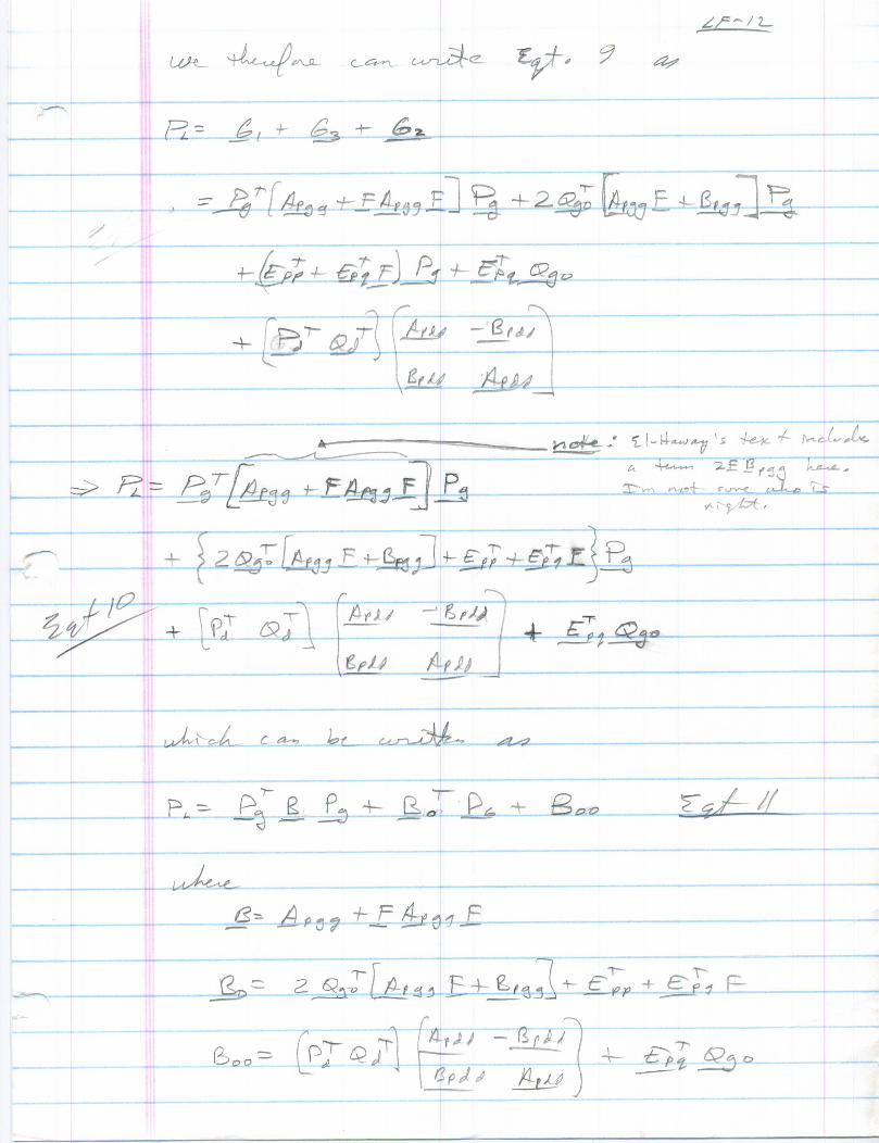
4.0 Using loss formula
The method of loss formula results in an
approximate expression given by
000 BPBPBPP GT
GTGL (17)
where PG is the vector of generation
Gm
GTG
P
P
P 1
(18)
Development of the coefficient matrices in (17)
has been done in several ways. The first edition of
the W&W text (1986) presented a method
developed by Meyer [2] in Appendix B of chapter
4; it was removed from the second edition.
I developed another method based on the work of
Kron, which is partially articulated in the book by
El-Harawry and Christenson, and attached to the
end of these notes.
15
Some important similarities in the methods:
1. Both are dependent on the following
assumptions:
Each bus can be clearly distinguished as
either a load bus or a generation bus.
Reactive generation varies linearly with
generation, i.e., Qgk=Qgo+fkPgk.
2. Both end up with expressions for PL of
the same form.
3. Both expressions for PL are dependent on
the elements of the Zbus matrix.
But there is one major difference between
the formulations in that Kron’s approach
makes no assumption regarding conforming
loads. However, the method of W&W
(Meyers) does, i.e., in Meyer’s approach, all
loads must increase or decrease uniformly.
We assume that we have the so-called B-
coefficients in the example which follows.

16

17

18

19

20

21
[1] A. Bergen and V. Vittal, “Power System Analysis,” Prentice-Hall, 2000.
[2] W. Meyer, “Efficient computer solution for Kron and Kron-Early Loss
Formulas,” Proc of the 1973 PICA conference, IEEE 73 CHO 740-1, PWR,
pp. 428-432.