ed 386: sciences math ematiques de paris centre mod ... · vent ^etre reconstruits et pr edits par...
TRANSCRIPT

Universite de Paris VI Pierre et Marie Curie
ED 386: Sciences mathematiques de Paris Centre
Modelisation mathematique du
role et de la dynamique
temporelle de la proteine p53
apres dommages a l’ADN induits
par les medicaments
anticancereux
THESE
presentee et soutenue publiquement le 1 Septembre 2015
pour l’obtention du diplome de
Doctorat en mathematiques appliquees
par
Jan Elias
apres avis des rapporteurs
Mark Chaplain
Roberto Natalini
devant le jury compose de
Luis Almeida ExaminateurMark Chaplain RapporteurJean Clairambault Directeur de theseMarie Doumic-Jauffret ExaminatriceRobin Fahraeus ExaminateurMarek Kimmel ExaminateurBenoıt Perthame Directeur de theseJack Tuszynski Examinateur
Laboratoire Jacques-Louis Lions INRIA (Mamba)


Pierre and Marie Curie University
DS 386: Mathematical Sciences of central Paris
Mathematical model of therole and temporal dynamics
of protein p53 after
drug-induced DNA damage
THESIS
presented and defended publicly on the 1st of September 2015
to obtain
PhD in Applied Mathematics
by
Jan Elias
after the review by
Mark ChaplainRoberto Natalini
in front of the jury composed of
Luis Almeida ExaminatorMark Chaplain ReviewerJean Clairambault Thesis AdvisorMarie Doumic-Jauffret ExaminatorRobin Fahraeus ExaminatorMarek Kimmel ExaminatorBenoıt Perthame Thesis AdvisorJack Tuszynski Examinator
Jacques-Louis Lions Laboratory INRIA (Mamba)


To my parents.To Eva who hung the moon.


Acknowledgement
First and foremost, I thank sincerely to Jean Clairambault and Benoıt Perthame for thegreat opportunity to study at the UPMC, for their indispensable guidance and assistance onwhat could otherwise have been an arduous road to finish this thesis. They are truly idealmentors, both of them demanding and generous: setting a high bar for performance, but alsoencouraging me to find my own way in terms of both topic and methods. I am indebted tothem for their advice and support over the past three years.
Thanks are due to the staff of the Laboratory J.-L. Lions as well as to Mme Nathalie Bontefor her kindness and help on a wide range of travel and other issues.
Special thanks are due to Silvia and Olivier for making our time in Paris more easier.
Along the way I would like to acknowledge at least few people I have met in France, namelyLuna, Rebecca, Nastasia, Faouzia, Sarah, Aurora, Andrada, Sarra, Rahma, Noemie, Wafaa,Carola, Tommaso, Alexander, Daisuke, Pierre J., Pierre L., Maxime, Thibault L., ThibaultB., Malik, Mamadou, Benjamin, Casimir, Xavier, Ange, Camille, Romain and those fromabroad, particularly Katharina, Romica, Sasha, Luyu, Bao and Gleb.
My thanks go to Antoine Le Hyaric for his assistance with FreeFem++.
Thanks go as well to Ayna and Mathias, Ramesh, Gopal and Mme Isabelle Bullier for some-times hilarious French classes.
I would like to thank my family, especially my mum, to all other family members and friendsfor their trust and encouragement over the past years.
I must conclude by thanking the person who helped me the most toward the completion ofthis thesis: Eva, a source of humour and good cheer, unconditional love and support.
i


Abstract
Various molecular pharmacokinetic–pharmacodynamic models have been proposed in thelast decades to represent and predict drug effects in anticancer therapies. Most of thesemodels are cell population based models since clearly measurable effects of drugs can beseen on populations of (healthy and tumour) cells much more easily than in individual cells.The actual targets of drugs are, however, cells themselves. The drugs in use either disruptgenome integrity by causing DNA strand breaks and consequently initiate programmed celldeath or block cell proliferation mainly by inhibiting proteins (cdks) that enable cells toproceed from one cell cycle phase to another. DNA damage caused by cytotoxic drugs orγ-irradiation activates, among others, the p53 protein-modulated signalling pathways thatdirectly or indirectly force the cell to make a decision between survival and death.
The thesis aims to explore closely intracellular pathways involving p53, “the guardian ofthe genome”, initiated by DNA damage and thus to provide oncologists with a rationale topredict and optimise the effects of anticancer drugs in the clinic. It describes p53 activationand regulation in single cells following their exposure to DNA damaging agents. We showthat dynamical patterns that have been observed in individual cells can be reconstructedand predicted by compartmentalisation of cellular events occurring either in the nucleus orin the cytoplasm, and by describing protein interactions, using both ordinary and partialdifferential equations, among several key antagonists including ATM, p53, Mdm2 and Wip1,in each compartment and in between them. Recently observed positive role of Mdm2 inthe synthesis of p53 is explored and a novel mechanism triggering oscillations is proposed.For example, new model can explain experimental observations that previous (not only our)models could not, e.g., excitability of p53.
Using mathematical methods we look closely on how a stimulus (e.g., γ-radiation or drugsused in chemotherapy) is converted to a specific (spatio-temporal) pattern of p53 whereassuch specific p53 dynamics as a transmitter of cellular information can modulate cellularoutcomes, e.g., cell cycle arrest or apoptosis. Mathematical ODE and reaction-diffusion PDEmodels are thus used to see how the (spatio-temporal) behaviour of p53 is shaped and whatpossible applications in cancer treatment this behaviour might have.
Protein-protein interactions are considered as enzyme reactions. We present some math-ematical results for enzyme reactions, among them the large-time behaviour of the reaction-diffusion system for the reversible enzyme reaction treated by an entropy approach. To ourbest knowledge this is published for the first time.
iii


Resume
Plusieurs modeles pharmacocinetiques-pharmacodynamiques moleculaires ont ete proposesau cours des dernieres decennies afin de representer et de predire les effets d’un medicamentdans les chimiotherapies anticancereuses. La plupart de ces modeles ont ete developpes auniveau de la population de cellules, puisque des effets mesurables peuvent y etre observesbeaucoup plus facilement que dans les cellules individuelles.
Cependant, les veritables cibles moleculaires des medicaments se trouvent au niveau de lacellule isolee. Les medicaments utilises soit perturbent l’integrite du genome en provoquantdes ruptures de brins de l’ADN et par consequent initialisent la mort cellulaire programmee(apoptose), soit bloquent la proliferation cellulaire, par inhibition des proteines (cdks) quipermettent aux cellules de proceder d’une phase du cycle cellulaire a la suivante en passantpar des points de controle (principalement en G1/S et G2/M). Les dommages a l’ADNcauses par les medicaments cytotoxiques ou la γ-irradiation activent, entre autres, les voiesde signalisation controlees par la proteine p53 qui forcent directement ou indirectement lacellule a choisir entre la survie et la mort.
Cette these vise a explorer en detail les voies intracellulaires impliquant la proteine p53,“le gardien du genome”, qui sont initiees par des lesions de l’ADN, et donc de fournir un ra-tionnel aux cancerologues pour predire et optimiser les effets des medicaments anticancereuxen clinique. Elle decrit l’activation et la regulation de la proteine p53 dans les cellules in-dividuelles apres leur exposition a des agents causant des dommages a l’ADN. On montreque les comportements dynamiques qui ont ete observes dans les cellules individuelles peu-vent etre reconstruits et predits par fragmentation des evenements cellulaires survenant apreslesion de l’ADN, soit dans le noyau, soit dans le cytoplasme. Ceci est mis en œuvre par ladescription du reseau des proteines a l’aide d’equations differentielles ordinaires (EDO) etpartielles (EDP) impliquant plusieurs agents dont les proteines ATM, p53, Mdm2 et Wip1,dans le noyau aussi bien que dans le cytoplasme, et entre les deux compartiments. Un rolepositif de Mdm2 dans la synthese de p53, qui a ete recemment observe, est explore et unnouveau mecanisme provoquant les oscillations de p53 est propose. On pourra noter en par-ticulier que le nouveau modele rend compte d’observations experimentales qui n’ont pas puetre entierement expliquees par les modeles precedents, par exemple, l’excitabilite de p53.
En utilisant des methodes mathematiques, on observe de pres la facon dont un stimulus(par exemple, une γ-irradiation ou des medicaments utilises en chimiotherapie) est convertien un comportement dynamique specifiques (spatio-temporel) de p53, en particulier que cesdynamiques specifiques de p53, comme messager de l’information cellulaire, peuvent modulerle cycle de division cellulaire, par exemple provoquant l’arret du cycle ou l’apoptose. Desmodeles mathematiques EDO et EDP de reaction-diffusion sont utilises pour examiner com-ment le comportement (spatio-temporel) de p53 emerge, et nous discutons des consequencesde ce comportement sur les reseaux moleculaires, avec des applications possibles dans letraitement du cancer.
Les interactions proteine–proteine sont considerees comme des reactions enzymatiques.On presente quelques resultats mathematiques pour les reactions enzymatiques, en particulieron etudie le comportement en temps grand du systeme de reaction-diffusion pour la reactionenzymatique reversible a l’aide d’une approche entropique. A notre connaissance, c’est lapremiere fois qu’une telle etude est publiee sur ce sujet.
v


Contents
Acknowledgement . . . . . . . . . . . . . . . . . . . . . . . . . . . . . . . . . . . . i
Abstract . . . . . . . . . . . . . . . . . . . . . . . . . . . . . . . . . . . . . . . . . . iii
Resume . . . . . . . . . . . . . . . . . . . . . . . . . . . . . . . . . . . . . . . . . . v
Abbreviations . . . . . . . . . . . . . . . . . . . . . . . . . . . . . . . . . . . . . . . xi
List of Figures . . . . . . . . . . . . . . . . . . . . . . . . . . . . . . . . . . . . . . xii
List of Tables . . . . . . . . . . . . . . . . . . . . . . . . . . . . . . . . . . . . . . . xiv
Introduction 1
Aims of the thesis . . . . . . . . . . . . . . . . . . . . . . . . . . . . . . . . . . . . 4
Organisation of the thesis . . . . . . . . . . . . . . . . . . . . . . . . . . . . . . . . 6
I Modelling p53 network 9
1 Biological background 11
1.1 The protein p53 in general . . . . . . . . . . . . . . . . . . . . . . . . . . . . . 11
1.2 p53, a transcription factor . . . . . . . . . . . . . . . . . . . . . . . . . . . . . 12
1.2.1 p53 forms tetramers for effective gene transcription . . . . . . . . . . . 12
1.2.2 p53 activation and regulation following genotoxic stress . . . . . . . . 13
1.2.3 p53 transcriptional activity towards proarrest and proapoptotic proteins 14
1.3 Ataxia Telangiectasia Mutated protein, ATM . . . . . . . . . . . . . . . . . . 14
1.3.1 ATM, a sensor of DSB . . . . . . . . . . . . . . . . . . . . . . . . . . . 14
1.3.2 Activity and regulation of ATM . . . . . . . . . . . . . . . . . . . . . 15
1.4 Mouse double minute 2protein, Mdm2 . . . . . . . . . . . . . . . . . . . . . . 16
1.4.1 Activity and regulation of Mdm2 . . . . . . . . . . . . . . . . . . . . . 17
1.5 The p53-Mdm2 auto-regulatory feedback loop . . . . . . . . . . . . . . . . . . 18
1.6 Wild-type p53-induced phosphatase 1, Wip1 . . . . . . . . . . . . . . . . . . . 19
1.7 Dynamics of the proteins in cancer cells following DNA damage . . . . . . . . 20
1.7.1 p53 dynamics measured over populations of cells . . . . . . . . . . . . 20
1.7.2 p53 oscillations in single cells . . . . . . . . . . . . . . . . . . . . . . . 21
1.7.3 Intracellular localisation and compartmentalisation . . . . . . . . . . . 22
2 Conceptual and Mathematical Foundations 25
2.1 Protein-protein interactions; post-translational modifications . . . . . . . . . 25
2.2 GRN for Wip1 and Mdm2; production and degradation of ATM and p53 . . 26
2.2.1 ATM activation in response to DSB . . . . . . . . . . . . . . . . . . . 28
2.2.2 Modelling p53 production . . . . . . . . . . . . . . . . . . . . . . . . . 30
2.2.3 Modelling p53 degradation . . . . . . . . . . . . . . . . . . . . . . . . 30
2.3 Diffusion of species in the cell . . . . . . . . . . . . . . . . . . . . . . . . . . . 31
2.4 Nucleocytoplasmic transmission, permeability . . . . . . . . . . . . . . . . . . 32
vii

2.5 Overview of other p53 models . . . . . . . . . . . . . . . . . . . . . . . . . . . 33
3 Physiological and compartmental ODE model for the p53 network 35
3.1 Introduction to the ODE model . . . . . . . . . . . . . . . . . . . . . . . . . . 35
3.2 ATM-p53-Mdm2-Wip1 compartmental model . . . . . . . . . . . . . . . . . . 36
3.2.1 Modelling ATM activation and deactivation . . . . . . . . . . . . . . . 36
3.2.2 Modelling p53 pathway by ODEs: assumptions . . . . . . . . . . . . . 39
3.2.3 Modelling p53 pathway by ODEs: equations . . . . . . . . . . . . . . . 41
3.2.4 Modelling p53 pathway by ODEs: one-compartment model . . . . . . 42
3.3 Numerical simulations and discussion . . . . . . . . . . . . . . . . . . . . . . . 43
3.3.1 The ODE model reproduces the oscillatory response of p53 to DNAdamage . . . . . . . . . . . . . . . . . . . . . . . . . . . . . . . . . . . 43
3.3.2 Bifurcation analysis of the system reveals two supercritical Hopf bifur-cation points that correlate with DNA damage levels . . . . . . . . . . 45
3.3.3 Two negative feedback loops and a compartmental distribution of cel-lular processes produce sustained oscillations . . . . . . . . . . . . . . 48
3.3.4 ATM threshold required for initiation of p53 pulses . . . . . . . . . . . 49
3.4 Conclusion from the ODE modelling . . . . . . . . . . . . . . . . . . . . . . . 51
4 Reaction-diffusion systems for protein networks 55
4.1 Introduction to spatio-temporal modelling . . . . . . . . . . . . . . . . . . . . 55
4.2 Reaction-diffusion models for protein intracellular networks . . . . . . . . . . 56
4.3 The Leloup–Goldbeter model for the Neurospora crassa circadian clock . . . 58
4.3.1 The frequency protein and circadian clock . . . . . . . . . . . . . . . . 58
4.3.2 Spatio-temporal Leloup–Goldbeter PDE model for FRQ . . . . . . . . 58
4.3.3 Discussion and conclusion: RD system for protein networks . . . . . . 60
5 Reaction-diffusion model for the p53 network 65
5.1 Rationale for a p53 PDE modelling . . . . . . . . . . . . . . . . . . . . . . . . 65
5.2 Modelling p53 dynamics: physiological ODE and reaction-diffusion PDE models 67
5.2.1 Mathematical formalism and notation . . . . . . . . . . . . . . . . . . 67
5.2.2 Compartmental ODE model . . . . . . . . . . . . . . . . . . . . . . . . 69
5.2.3 Reaction-diffusion PDE model . . . . . . . . . . . . . . . . . . . . . . 69
5.2.4 Nucleocytoplasmic transmission BC: Kedem–Katchalsky boundaryconditions . . . . . . . . . . . . . . . . . . . . . . . . . . . . . . . . . . 71
5.2.5 Diffusion and permeability coefficients for the RD model . . . . . . . . 72
5.2.6 Nondimensionalisation . . . . . . . . . . . . . . . . . . . . . . . . . . . 73
5.2.7 Numerical simulations of PDEs in 2 and 3 dimensions . . . . . . . . . 74
5.3 Numerical simulations of PDEs: results . . . . . . . . . . . . . . . . . . . . . 75
5.3.1 Oscillations of p53 in the PDE model . . . . . . . . . . . . . . . . . . 75
5.3.2 Parameter sensitivity analysis: activation “stress” signal E . . . . . . 76
5.3.3 Parameter sensitivity analysis: diffusivity and permeability parameters 80
5.3.4 Sole p53-Mdm2 negative feedback does not trigger oscillations . . . . . 81
5.3.5 One compartmental model does not trigger oscillations . . . . . . . . . 82
5.3.6 Oscillations in cells of complicated structures . . . . . . . . . . . . . . 83
5.4 Discussion and conclusions from the PDE model #1 . . . . . . . . . . . . . . 84
viii

6 Novel mechanism for p53 oscillations: positive role of the negative regulatorMdm2 916.1 Mdm2’s dual function toward p53 in DDR . . . . . . . . . . . . . . . . . . . . 916.2 A novel mechanism for p53 oscillations . . . . . . . . . . . . . . . . . . . . . . 93
6.2.1 Modelling Mdm2’s dual function: assumptions . . . . . . . . . . . . . 956.2.2 Modelling Mdm2’s dual function: RD equations . . . . . . . . . . . . . 976.2.3 Numerical simulations . . . . . . . . . . . . . . . . . . . . . . . . . . . 98
6.3 Excitability of p53 . . . . . . . . . . . . . . . . . . . . . . . . . . . . . . . . . 1016.4 Discussion and conclusions from the PDE model #2 . . . . . . . . . . . . . . 105
7 Summary of the p53 modelling and follow-up work 1097.1 Physiological ODE and PDE models for p53 . . . . . . . . . . . . . . . . . . . 1097.2 p53 as a chemotherapeutic target . . . . . . . . . . . . . . . . . . . . . . . . . 1107.3 p53 dynamics in blocking proliferation and launching apoptosis . . . . . . . . 1117.4 Cancer therapies and PK–PD models . . . . . . . . . . . . . . . . . . . . . . . 1127.5 Other concluding notes . . . . . . . . . . . . . . . . . . . . . . . . . . . . . . . 113
II Modelling enzyme reaction 115
8 Beyond the enzyme reaction model 1178.1 Introduction to enzyme reactions . . . . . . . . . . . . . . . . . . . . . . . . . 1178.2 Michaelis-Menten Law and ODE system . . . . . . . . . . . . . . . . . . . . . 1188.3 Reaction-diffusion system for the reversible enzyme reaction . . . . . . . . . . 121
8.3.1 Entropy, entropy dissipation and first estimates . . . . . . . . . . . . . 1238.3.2 L2(logL)2 estimates . . . . . . . . . . . . . . . . . . . . . . . . . . . . 1248.3.3 L∞ estimates in 1-3D: bootstrapping argument . . . . . . . . . . . . . 1258.3.4 Other properties of the EnR system . . . . . . . . . . . . . . . . . . . 1268.3.5 Large-time behaviour: convergence in relative entropy . . . . . . . . . 128
Appendix 139Appendix A: Duality principle . . . . . . . . . . . . . . . . . . . . . . . . . . . . . 139Appendix B: Existence of a solution to the EnR RD by the Rothe method . . . . . 141
Rothe method for an abstract parabolic problem . . . . . . . . . . . . . . . . 141Existence of the global weak solution to (8.20)-(8.22) by the Rothe method . 143FreeFem++ code for the reversible EnR system . . . . . . . . . . . . . . . . . 148
Bibliography 155
ix


Abbreviations
[ · ], molar concentrationATM, Ataxia Telangiectasia Mutated proteindoxo, doxorubicinBC, boundary condition(s)BL, Burkitt lymphoma cellsDA-1, murine lymphoma cellsDDE, Delayed Differential EquationsDDR, DNA damage responseDNA, Deoxyribonucleic acidDSB, double strand breaksER, endoplasmic reticulumEnR, enzyme reactionFRQ, Frequency proteinGNR, gene regulatory networkIR, irradiation (γ-irradiation)LMA, Law of Mass ActionLys, lysine residueMdm2, Mouse double minute 2 (Hdm2 in human cells, hereafter Mdm2 only)MdmX, Mouse double minute 4 homolog (HdmX in human cells, hereafter MdmX only)ML-1 myeloid leukaemia cellsNCS, neocarzinostatinNES, nuclear export signalNLS, nuclear localisation signalsODE, Ordinary Differential EquationsOsA-CL, osteosarcoma cell linep53, tumour protein p53p53-P, phosphorylated p53 protein (this notation is applied for other proteins)PDE, Partial Differential EquationsPK–PD, pharmacokinetic–pharmacodynamicPTEN, Phosphatase and TENsin homologQSSA, quasi-steady-state approximationRD, reaction-diffusionRKO, colorectal carcinoma cellsSer, serine residueSSB, single strand breakst1/2, half-life of a protein/mRNATF, transcription factorThr, threonine residueWip1, Wild-type p53-induced phosphatase 1wm, wortmanninwt, wild type
xi

List of Figures
1 p53, the guardian of the genome . . . . . . . . . . . . . . . . . . . . . . . . . 2
2 Chemotherapy at the single cell and cell population level . . . . . . . . . . . . 2
3 ATM-p53-Mdm2-Wip1 dynamics . . . . . . . . . . . . . . . . . . . . . . . . . 3
1.1 ATM activation after DNA damage . . . . . . . . . . . . . . . . . . . . . . . . 15
1.2 p53-Mdm2 auto-regulatory feedback . . . . . . . . . . . . . . . . . . . . . . . 18
1.3 Experimental data: Induction of p53 and Mdm2 in ML-1 cells . . . . . . . . . 20
1.4 Experimental data: Induction of p53 and Mdm2 in DA-1 and ML-1 cells . . . 21
1.5 Experimental data: Damped oscillations of p53 and Mdm2 in NIH 3T3 andMCF-7 cells . . . . . . . . . . . . . . . . . . . . . . . . . . . . . . . . . . . . . 22
1.6 Experimental data: Time-lapse imaging of oscillations of p53 and Mdm2 in asingle cell . . . . . . . . . . . . . . . . . . . . . . . . . . . . . . . . . . . . . . 23
2.1 ATM activation and inactivation in DDR . . . . . . . . . . . . . . . . . . . . 29
2.2 Schematic representation of a 2D cell used in the p53 modelling . . . . . . . . 30
2.3 Passive transport throughout the nuclear membrane . . . . . . . . . . . . . . 32
3.1 Migration of the species between the nucleus and cytoplasm in the ODE model 40
3.2 ODE model: Nuclear and cytoplasmic concentrations . . . . . . . . . . . . . . 43
3.3 ODE model: Phase planes of p53-P vs. ATM-P and p53-P vs. Mdm2 . . . . 44
3.4 ODE model: Phase planes of ATM-P vs. Wip1 and p53-P vs. Wip1 . . . . . 44
3.5 ODE model: Duration of 15 pulses in the p53-P concentration . . . . . . . . 45
3.6 ODE model: A pair of complex eigenvalues for the existence of two Hopfbifurcation points and periods of stable limit cycles maintained between theseHopf points for varying E . . . . . . . . . . . . . . . . . . . . . . . . . . . . . 46
3.7 ODE model: Other bifurcation diagrams . . . . . . . . . . . . . . . . . . . . . 47
3.8 ODE model: Concentrations of the species for small and large E . . . . . . . 48
3.9 ODE model: Concentrations of the species after inhibition of ATM-P followingone full pulse . . . . . . . . . . . . . . . . . . . . . . . . . . . . . . . . . . . . 49
3.10 ODE model: Concentration of the species when kub = 0 and in the case ofone-compartmental model . . . . . . . . . . . . . . . . . . . . . . . . . . . . . 50
3.11 ODE model: Evolution of the Hopf points with varying ATMTOT , bifurcationdiagram . . . . . . . . . . . . . . . . . . . . . . . . . . . . . . . . . . . . . . . 51
3.12 ODE model: Other plots confirming the need of both negative feedbacks foroscillations . . . . . . . . . . . . . . . . . . . . . . . . . . . . . . . . . . . . . 53
4.1 Schematic representation of a 2D cell . . . . . . . . . . . . . . . . . . . . . . . 57
4.2 FRQ PDE model: solutions and phase planes . . . . . . . . . . . . . . . . . . 61
4.3 Schematic representation of a 2D cell used in the FRQ modelling . . . . . . . 62
5.1 p53-Mdm2 and ATM-p53-Wip1 negative feedback loops in the PDE Model 1 66
5.2 p53 dynamics in normal conditions in the PDE Model 1 . . . . . . . . . . . . 67
5.3 p53 dynamics in response to DNA damage in the PDE Model 1 . . . . . . . . 68
5.4 2D and 3D triangulations used in modelling . . . . . . . . . . . . . . . . . . . 74
5.5 p53 PDE Model 1: 2D and 3D nuclear concentrations in normal conditions,E = 0 . . . . . . . . . . . . . . . . . . . . . . . . . . . . . . . . . . . . . . . . 76
5.6 p53 PDE Model 1: 2D and 3D nuclear and cytoplasmic concentrations in theDDR, E = 1 . . . . . . . . . . . . . . . . . . . . . . . . . . . . . . . . . . . . . 77
5.7 p53 2D PDE Model 1: Phase plane of p53 vs. Mdm2; half-life of p53 . . . . . 78
xii

5.8 p53 3D PDE Model 1: Phase plane of p53 vs. Mdm2; half-life of p53 . . . . . 785.9 p53 3D PDE Model 1: visualisation of p53 concentration . . . . . . . . . . . . 795.10 p53 3D PDE Model 1: visualisation of Mdm2 concentration . . . . . . . . . . 795.11 p53 2D PDE Model 1: Bifurcation diagram for nuclear p53 with respect to E 805.12 p53 2D PDE Model 1: Solutions in various cases demonstrating inability of
the sole p53-Mdm2 negative feedback to produce sustained oscillations . . . . 835.13 p53 2D PDE Model 1: Solution of the one-compartmental model . . . . . . . 845.14 HeLa cell used in the modelling . . . . . . . . . . . . . . . . . . . . . . . . . . 855.15 p53 2D PDE Model 1: Nuclear and cytoplasmic concentrations in the (HeLa)
cell of complicated structure . . . . . . . . . . . . . . . . . . . . . . . . . . . . 865.16 p53 2D PDE Model 1: 2D visualisation of p53 in the (HeLa) cell of complicated
structure . . . . . . . . . . . . . . . . . . . . . . . . . . . . . . . . . . . . . . . 875.17 p53 2D PDE Model 1: 2D visualisation of Mdm2 in the (HeLa) cell of compli-
cated structure . . . . . . . . . . . . . . . . . . . . . . . . . . . . . . . . . . . 88
6.1 Positive effect of Mdm2 and MdmX towards p53 . . . . . . . . . . . . . . . . 936.2 A simplified positive effect of Mdm2 towards p53 . . . . . . . . . . . . . . . . 946.3 Scheme of the cell used in Model 2 . . . . . . . . . . . . . . . . . . . . . . . . 956.4 p53 Model 2: Nuclear concentrations in the DDR, E = 1 . . . . . . . . . . . . 1006.5 p53 Model 2: Phase plane of p53 vs. Mdm2; half-life of p53 . . . . . . . . . . 1016.6 p53 Model 2: Nuclear concentrations in the DDR, E = 1 and ka = 0 . . . . . 1026.7 p53 Model 2: Nuclear concentrations in the DDR, E = 1 and ktp-1 = ktp-2 = 1 1026.8 p53 Model 2: Nuclear concentration in normal conditions, E = 0; dependence
of the solution on varying E . . . . . . . . . . . . . . . . . . . . . . . . . . . . 1036.9 Excitability of p53 in response to DSB and SSB . . . . . . . . . . . . . . . . . 1036.10 Excitability of p53 in Model 2 . . . . . . . . . . . . . . . . . . . . . . . . . . . 1046.11 Excitability of p53 in Model 1 and in Model 2 when ka = 0 . . . . . . . . . . 1056.12 p53-Mdm2 and ATM-Mdm2-p53-Wip1 negative feedback loops in Model 2 . . 106
7.1 Dynamics of p53 as a marker of cell fate . . . . . . . . . . . . . . . . . . . . . 111
8.1 Graph of the function Φ . . . . . . . . . . . . . . . . . . . . . . . . . . . . . . 1298.2 Graphs of the functions 3(
√a−√b)2, (a− b)(log a− log b) and 7(
√a−√b)2 . 132
8.3 Rothe’s interpolants . . . . . . . . . . . . . . . . . . . . . . . . . . . . . . . . 1428.4 Example of 2D simulation of the reversible enzyme reaction . . . . . . . . . . 147
xiii

List of Tables
2.1 Half-lives and degradation rates for the species . . . . . . . . . . . . . . . . . 28
3.1 Parameters for the compartmental ODE model . . . . . . . . . . . . . . . . . 54
4.1 Parameters for the FRQ PDE model . . . . . . . . . . . . . . . . . . . . . . . 60
5.1 Kedem–Katchalsky boundary conditions for the p53 PDE Model 1 . . . . . . 725.2 Diffusion and permeability rates for the species . . . . . . . . . . . . . . . . . 735.3 Table of diffusivities admissible for oscillations . . . . . . . . . . . . . . . . . 815.4 Table of permeabilities admissible for oscillations . . . . . . . . . . . . . . . . 825.5 Parameters for the p53 PDE Model 1 . . . . . . . . . . . . . . . . . . . . . . 90
6.1 Kedem–Katchalsky boundary conditions for the p53 PDE Model 2 . . . . . . 996.2 Parameters for the p53 PDE Model 2 . . . . . . . . . . . . . . . . . . . . . . 107
8.1 Relations between µi for i ∈ S,E,C, P . . . . . . . . . . . . . . . . . . . . . 135
xiv

Introduction
“Beauty is the first test. There is no permanent placein the world for ugly mathematics.”
– G. H. Hardy (1877–1947)
Shortly after disruption of the integrity of the genome of a cell by various pharmacologicalagents or ionising radiation, the cell responds dynamically by activating a variety of recog-nition and repair proteins recruited to DNA damage sites, by initiating various signallingpathways leading either to cell cycle arrest and parallel DNA repair, permanent cell cyclearrest or cell death. Among these pathways, the most important ones involve the tumoursuppressor protein p53, the so-called guardian of the genome, that initiates expression ofthose genes that ultimately govern cell cycle arrest, DNA damage repair and apoptosis, Fig-ure 1, involving the production of proteins of concentrations proportionally related to theconcentrations of p53. At the cell population level (i.e., tissues, organs, whole human body)pharmacokinetics–pharmacodynamics (PK–PD) modelling has been broadly used to fully de-scribe absorption, distribution, metabolism, excretion and toxicity of anticancer drugs. Muchless, however, has been done at the single cell (molecular) level to describe drug effects, con-sidering that individual cells are the actual targets of drug administration [29]. Some drugs(e.g., radiomimetic drugs including doxorubicin, bleomycin or etoposide, alkylating agentsor oxaliplatin) directly cause DNA double strand breaks (DSB), others target essential cellcycle enzymes (such as topoisomerases or thymidylate synthase), leading to the productionof abnormal DNA and forcing the cell to start the process of apoptosis, at least when DNAcannot be repaired [30].
Thus, to reproduce more realistically drug effects in cancer treatments, as described byPK–PD models with DNA damage as output, it may be helpful to include in existing modelsprocesses that appear in individual cells after DNA insult, beginning with a proper under-standing of p53 activation and activity in single cells, with the perspective of subsequentintegration of such activity into a cell fate decision process, Figure 2. Bearing in mind thatp53 is inactive due to its gene mutations in around 50% of tumour cells, with the rate varyingfrom 10–12% in leukaemia, 38–70% in lung cancers to 43–60% in colon cancers, etc. [111],the approaches involving processes occurring in individual cells with the dominant role of p53can contribute to establishing new cancer therapies that could either restore p53’s lost func-tionality or substitute for it in the activation of subsequent proteins in various p53-initiatedpathways.
In this modelling enterprise, the main object of interest at the single cell level is thus theprotein p53, its activation and its activity on proarrest and proapoptotic genes that enablethe cell to make a decision between cell cycle arrest and DNA repair, permanent arrest ofcell growth (so-called senescence) and cell death (apoptosis), Figure 1. Interestingly, the firstp53-transcription independent wave of cells committing apoptosis in response to γ-irradiationis observed 30 minutes after DNA damage by rapid accumulation of p53 in the mitochondria.The second wave comes after a longer time phase and the decision of the cell to undergo
1

2
Figure 1. p53, the guardian of the genome: p53 responds to a variety of stress stimuliinitiating cell cycle arrest, DNA damage repair, apoptosis or senescence [79, 147, 149].
Chemotherapy
cell population
levels
single cell
levels
?
molecular e!ects of
drugs
measurable e!ects
of drugs, PK-PD models
(p53 mediated cell cycle arrest,
proliferation and death)
Figure 2. Action of chemotherapeutic agents is exploited in individual cells. Whilst thereexist several PK–PD models for effects of a chemotherapy at the cell population level, muchless is known about how specific drugs act in single cells.
apoptosis in this wave is determined by the concentrations of both proapoptotic and proarrestproteins, the expression of which is modulated by p53 [73, 111]. However, different sorts ofsuch apoptotic proteins are produced, in a cell-stress, cell-type and tissue-type dependentmanner. Various post-translational modifications, interactions of p53 with over 100 cellularcofactors and p53 cellular location have effects on determining what kind of proteins andwhen these proteins are produced [111].
The signalling of p53 in response to a variety of stimuli is complex, involving hundreds of
3
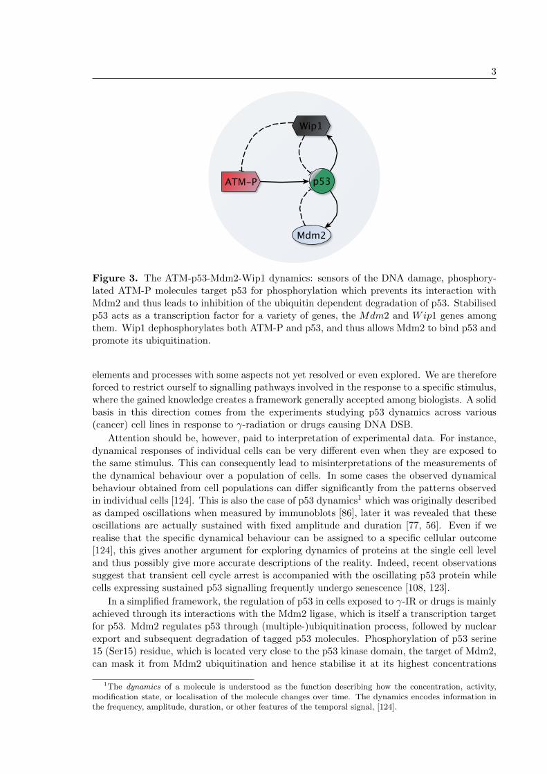
Figure 3. The ATM-p53-Mdm2-Wip1 dynamics: sensors of the DNA damage, phosphory-lated ATM-P molecules target p53 for phosphorylation which prevents its interaction withMdm2 and thus leads to inhibition of the ubiquitin dependent degradation of p53. Stabilisedp53 acts as a transcription factor for a variety of genes, the Mdm2 and Wip1 genes amongthem. Wip1 dephosphorylates both ATM-P and p53, and thus allows Mdm2 to bind p53 andpromote its ubiquitination.
elements and processes with some aspects not yet resolved or even explored. We are thereforeforced to restrict ourself to signalling pathways involved in the response to a specific stimulus,where the gained knowledge creates a framework generally accepted among biologists. A solidbasis in this direction comes from the experiments studying p53 dynamics across various(cancer) cell lines in response to γ-radiation or drugs causing DNA DSB.
Attention should be, however, paid to interpretation of experimental data. For instance,dynamical responses of individual cells can be very different even when they are exposed tothe same stimulus. This can consequently lead to misinterpretations of the measurements ofthe dynamical behaviour over a population of cells. In some cases the observed dynamicalbehaviour obtained from cell populations can differ significantly from the patterns observedin individual cells [124]. This is also the case of p53 dynamics1 which was originally describedas damped oscillations when measured by immunoblots [86], later it was revealed that theseoscillations are actually sustained with fixed amplitude and duration [77, 56]. Even if werealise that the specific dynamical behaviour can be assigned to a specific cellular outcome[124], this gives another argument for exploring dynamics of proteins at the single cell leveland thus possibly give more accurate descriptions of the reality. Indeed, recent observationssuggest that transient cell cycle arrest is accompanied with the oscillating p53 protein whilecells expressing sustained p53 signalling frequently undergo senescence [108, 123].
In a simplified framework, the regulation of p53 in cells exposed to γ-IR or drugs is mainlyachieved through its interactions with the Mdm2 ligase, which is itself a transcription targetfor p53. Mdm2 regulates p53 through (multiple-)ubiquitination process, followed by nuclearexport and subsequent degradation of tagged p53 molecules. Phosphorylation of p53 serine15 (Ser15) residue, which is located very close to the p53 kinase domain, the target of Mdm2,can mask it from Mdm2 ubiquitination and hence stabilise it at its highest concentrations
1The dynamics of a molecule is understood as the function describing how the concentration, activity,modification state, or localisation of the molecule changes over time. The dynamics encodes information inthe frequency, amplitude, duration, or other features of the temporal signal, [124].

4
[42, 43, 147]. In response to DSB, p53 can be phosphorylated on Ser15 in three independentways, one of which is phosphorylation by the ATM kinase [147]. The Wip1 phosphatase isanother p53 target which acts in the pathway as a regulator; particularly, it dephosphorylatesboth ATM and p53, rendering them inactive, whence Wip1 closes negative feedback loopsbetween these proteins as it is schematically shown on Figure 3. Recently, these four proteinshave been shown to represent sufficient and necessary elements in the p53 (minimal) networkwhich can produce p53 oscillations following DNA damage [15].
The ligase Mdm2 primarily acts as a negative regulator of p53 establishing homeostasisin DNA damage response (DDR). Recently published studies show that following ATM-dependent phosphorylation of Mdm2, the phosphorylated Mdm2 was observed not to targetp53 for degradation but rather, and somehow surprisingly, to enhance p53 synthesis. Thusit can function as a positive regulator by undergoing certain post-translational modifications[54, 96].
The simplified p53 network relying on the p53-Mdm2 and ATM-p53-Wip1 negative feed-backs became basis for three articles where we continuously embedded a physiological andcompartmental ODE model from [47] into a spatio-temporal PDE model [46, 45]2. BothODE and PDE models were aimed to reproduce basic biological observations as described inmore details below. The third article [45] serves as an introduction into modelling protein(namely, p53 and FRQ) networks by reaction-diffusion equations which are largely over-looked by mathematicians and system biologists. In the reaction-diffusion PDE models,reaction terms describe protein-protein interactions and gene regulatory networks and diffu-sions naturally stand for migration of the species across and in between the two main cellularcompartments: nucleus and cytoplasm.
[45] J. Elias and J. Clairambault. Reaction-diffusion systems for spatio-temporalintracellular protein networks: A beginners guide with two examples. Computationaland Structural Biotechnology Journal, 10(16):12–22, 2014.
[46] J. Elias, L. Dimitrio, J. Clairambault, and R. Natalini. The dynamics ofp53 in single cells: physiologically based ODE and reaction–diffusion PDE models.Physical Biology, 11(4):045001, 2014.
[47] J. Elias, L. Dimitrio, J. Clairambault, and R. Natalini. The p53 protein andits molecular network: Modelling a missing link between DNA damage and cell fate.Biochimica et Biophysica Acta (BBA) - Proteins and Proteomics, 1844(1, PartB):232–247, 2014.
Aims of the thesis
With the perspective of future (biological and pharmacological) applications, we consider insilico the p53 protein and its signalling in response to DNA damage, particularly to DSBcaused by agents such as γ-radiation or drugs, at the single cell level. The principal aim ofthe thesis lies in a study of spatio-temporal dynamics of p53 in an individual cell and closeexamination of its dynamical patterns depending on a physical structure of the cell as wellas other factors such as DNA damage dose.
2The articles are ordered from the most recent to the earliest.

5
Several aims are followed in the thesis. Among them,
• first and foremost, we aim to model p53 response to DNA damage more plausibly withrespect to the relevant biological observations (discussed in the biological overview)including
– a DNA damage-transmitting-signal (i.e., ATM) which is able to sense the presenceof DSB and transmit the signal to p53, and regulators of p53 enabling to maintainhomeostasis in the DDR (i.e., Mdm2 and Wip1), in their dynamical states ratherthan being constant substrates,
– spatial representation of cells and thus differentiation of processes in the p53 path-way taking place either in the nucleus or in the cytoplasm; this gives a rise tophysiologically more relevant cellular framework for the modelling; then
• we aim to provide an analysis of the models with respect to the extent of DNA damageand examine thus p53 dynamical responses to different doses of stimulus,
• we aim to provide an analysis of the models with respect to spatial variables and examinethus roles of the spatial structure of a cell in maintaining specific patterns in the p53response,
since once we are successful in achieving of these goals, the model simulating realistic be-haviour of p53 could become attractive for biologists (which is another “hidden” aim of thiswork).
We try to answer several other questions that can further contribute to a more detailedunderstanding of the complex p53 dynamics in cancer cells, which are exposed to damagingagents. Some of these questions are:
• What is the role of the sole p53-Mdm2 negative feedback in the p53 response? Can itbe the only “force” triggering oscillations?
• Can a positive role of Mdm2 towards synthesis of p53 provide an independent mecha-nism for the oscillatory behaviour of p53?
• Based on the models, could we propose a molecular mechanism (which is unknown sofar) underlying phenomena of the excitability of p53 in response to DSB?
• By assuming biological hypotheses giving into relation p53 patterns with a specific(irreversible) fate outcome, can the models be used to predict molecular targets incancer treatment which, after being hit by a known or hypothetical pharmacologicalagent, could establish the phenotype in question? This brings us to:
• Could the proposed models be used to exploit dynamics of pharmacological agents(currently used in clinical trials) or possibly to direct biochemists in the investigationfor new chemicals; to extend current PK–PD models with a molecular module whichwould describe the action of these agents more properly?
Except for all these mathbio aspects which rely on modelling, we consider some math-ematical problems related to ODE and PDE systems for enzyme reactions. Although theenzyme reactions represent fundamental basis for our modelling, the particular results stayindependent of the mathbio part.

6
Organisation of the thesis
The thesis consists of two autonomous parts: the first and most extensive part is devoted tothe modelling p53 network, its activation and regulation in response to DNA damage. Thispart spreads over the first seven chapters which describe a “genealogy” of our mathematicalmodelling starting with biological and mathematical foundations, passing through a compart-mental ODE model, two reaction-diffusion PDE models for p53 and finishing with generalconclusions about p53 dynamics and its applications to cell fate decisions. Both PDE modelsexploit different mechanisms for triggering p53 oscillations. The second part consisting of onechapter only is dedicated to some issues related to enzyme reactions. Rather than being acompact text, this chapter is a collection of two independent results: one for an ODE systemmodelling irreversible enzyme reaction, the other one for a reaction-diffusion PDE system forthe reversible enzyme reaction. What follows are short descriptions of the chapters.
Part I.
• Chapter 1 highlights general biological knowledge about the p53 protein andother proteins regulating response of p53 to DNA damage including ATM, Mdm2and Wip1. Dynamics of the proteins in cancers cells following genotoxic insultas well as p53-Mdm2 auto-regulatory feedback and observations from single cellexperiments are briefly overviewed.
• Chapter 2 introduces basic mathematical concepts used in modelling. The focusis on the Law of Mass Action applied to enzyme reaction as a prototypic reactionrepresenting protein-protein interactions. Simple gene regulatory networks forMdm2 and Wip1 proteins as well as induction and degradation of ATM and p53are discussed. Further, transmission of the species throughout the membranes andissues around intracellular movement of the species are studied. The chapter isconcluded with a review of other existing models simulating p53 dynamics.
• Chapter 3 presents a physiological and compartmental ODE model for p53 dy-namics following DNA damage. The model is based on the p53-Mdm2 negativefeedback complemented with another negative feedback between ATM and Wip1.Analysis with respect to the DNA damage signal is provided.
• Chapter 4 gives a general introduction into modelling protein networks by spatio-temporal reaction-diffusion equations. As an example, the dynamics of the Fre-quency (FRQ) protein from the well known Leloup–Goldbeter circadian clock ODEmodel is examined in new spatial settings.
• Chapter 5 focuses on a reaction-diffusion model for the p53 protein and its sig-nalling in an individual cell after DNA damage. This physiologically more plau-sible model considers the two negative feedback loops from the ODE model. Thereaction-diffusion PDE model is examined with respect to several biological obser-vations. Its analysis with respect to the DNA damage signal and spatial parametersis given.
• Chapter 6 presents a novel mechanism for p53 oscillations relying on a positiverole of Mdm2 towards p53. It is shown that this dual (positive vs. negative) func-tion of Mdm2 depending on Mdm2’s phosphorylation status can create a molecularframework generating p53 oscillations as well as it can explain the excitability ofp53 in response to DSB.

7
• Chapter 7 summarises all the work done in the previous chapters. It attemptsto relate the developed models with the possible applications in cell fate decisionsas well as PK–PD models.
Part II.
• Chapter 8 considers two autonomous problems related to the enzyme reaction.In particular, the validity of the quasi-steady state approximation is given andthe large time behaviour of a reaction-diffusion system for the reversible enzymereaction is studied.

8

Part I
Modelling p53 network
9


1
Biological background
Our main object, the tumour suppressor p53, is found at low levels in normal cellsunder normal conditions. In response to a stimulus, it is activated and acts pri-marily as a transcription factor for many other genes which, if possible, silencefluctuations caused by the stimulus, if not possible, initiate processes forcing cellsto trigger an irreversible state such as apoptosis or senescence to prevent the de-velopment of cancer. The biological knowledge about the p53 protein has becamevery broad since its discovery, thus in the following sections we give a summary ofthe basic properties of p53, its functional activity towards upstream and downstreamsubstrates, its activation in response to genotoxic stress and other biological featureswhich we think are important to mention. Other key players in the p53 network, inparticular, ATM, Mdm2 and Wip1 are also reviewed in this chapter.Dynamics of the p53 protein in cancers cells is of special interest for us with respectto possible future applications of our models. In this chapter we thus depict severalobservations of the dynamics of p53 and other proteins following DNA damage (suchas DSB) caused by irradiation or drugs.
Organisation of the chapter is as follows: Sections 1.1-1.6 present short descriptionsof the main antagonists, namely, p53, ATM, Mdm2 and Wip1. The p53-Mdm2auto-regulatory feedback is described in Section 1.5. The dynamics of the proteinsincluding single cells experiments are reviewed in Section 1.7.
1.1 The protein p53 in general
The protein p53 as a tumour suppressor controls transitions from G1 to S and from G2to mitosis cell cycle phases during a tissue development and subsequent tissue regenerationrelying on the divisions of cells at mitosis [27]. The p53 protein can respond to abnormaldevelopmental pathways triggered by oncogene or tumour suppressor gene mutations, thuspreventing the cell from turning it into a malignant cell [88]. It is also activated wheneverthe DNA is exposed to various stress conditions such as ionising γ-radiation, UV or variousdrugs in chemotherapies causing DNA damage and also by agents which do not cause DNAdamage, for example, hypoxia, starvation, heat and cold, see e.g. [79, 147, 149] and Figure 1.In the response to these stresses, p53 transcriptionally activates a bench of proarrest andproapoptotic proteins leading either to cell cycle arrest (and thus it enables repair processesto fix the DNA damage), senescence or apoptosis [111], apparently, with no ability of p53 topreferentially activate proarrest target genes rather than proapoptotic genes and vice-versadue to the (higher/lower) affinity of p53 for these genes [73].
11
12 1. Biological background
Although mutations of the p53 gene primarily do not cause cancer, inactivation of its tran-scriptional activity, mostly due to missense mutations located in the DNA-binding domain,can lead to failures in the prevention of unnatural growth whenever some other mutations ofgenes causing uncontrolled growth occur [66]. p53 mutations are common in human cancers(they occur in about 50% of mammalian cancer cells) and are frequently associated withaggressive disease courses and drug resistance, for example, patients with AML at diagnosis(with mutations in the p53 gene of 10%-15% initially) [162]. Patients with rare p53 genegerm line mutations known as Li-Fraumeni syndrome have an approximately 90% lifetimerisk of developing cancer (50% before the age of 40 years) [90]. Interestingly, even when tran-scriptionally inactivated by a point mutation at the DNA-binding domain, about 70–80% ofhuman carcinomas express such p53 mutants at high levels [154, 80]. Accumulation of highlevel mutant p53 expression during tumour development thus suggests that it may positivelyaffect proliferation of cancer cells, [118] and citations therein.
In many other human tumours with wild-type and thus transcriptionally active p53, p53activity is suppressed by its regulators Mdm2 and Wip1 which are over-expressed in thesecancer cell lines. The p53 gene remains in its wild-type configuration, likely because the over-expression of the negative regulators decreases the selective pressure for direct mutationalinactivation of the p53 gene, [92, 106] and citations therein.
The p53 protein is extensively studied protein and there can be found thousands of articlesdescribing p53 signalling or reviewing it and its functions in more details (for reviews see, forinstance, Vogelstein, Lane & Levine [147], Murray-Zmijewski, Slee & Lu [111] and Vousden& Lane [149]). In the following sections we point out only the most important facts that arefurther recalled in the modelling.
1.2 p53, a transcription factor
The p53 gene product functions as a transcription factor. The wild-type p53 protein can bindto specific nucleotide sequences, also called p53-responsive elements. When these elementsare close to a promoter they stimulate expression in a p53-dependent manner both in vivoand in vitro. Mutations in the p53 gene can still produce p53 proteins that however fail tobind to DNA and fail to transcriptionally activate p53-responsive genes, [154] and citationtherein.
Functional activity of p53 follows its nuclear stabilisation which means that for a certainamount of time p53 is able to retain its structural conformation preventing it from degrada-tion or aggregation and to retain its activity when it is exposed to manipulations [147, 42].The structural conformation relies on a series of post-translational modification (e.g., phos-phorylation at Ser15) as discussed in Section 1.2.2 and formation of higher order homodimersas described firstly in Section 1.2.1.
1.2.1 p53 forms tetramers for effective gene transcription
The p53 protein forms tetramers and the tetramer formation is essential for its function [53,66]. Indeed, tetrameric p53 cooperatively binds to DNA [152] and tetramerisation mediatedby the tetramerisation domain regulates the DNA binding activity of p53 [139]. However, atlow levels or when p53 moves across the nucleus, p53 is likely in the dimeric form [64, 152].
Using three-dimensional structural analysis it was found that the residues containingthe putative nuclear export signal (NES) are suitable substrates for the export receptorswhenever p53 is in the monomeric or dimeric state. Tetrameric p53 cannot be exported fromthe nucleus since the NES lies within the tetramerisation domain and is thus hidden from the

1.2. p53, a transcription factor 13
export receptors [139]. Notably, the domain of p53, which is required for oligomerisation, isalso crucial for Mdm2 binding and Mdm2-dependent ubiquitination of p53 [106].
Thus, the tetramerisation of p53 molecules contributes to the nuclear accumulation andstabilisation of p53.
1.2.2 p53 activation and regulation following genotoxic stress
The tumour suppressor protein p53 can be activated in at least three independent ways: DNAdamage caused, for example, by ionising radiation or electromagnetic γ-radiation, with initialactivation of ATM and Chk2 proteins; aberrant growth signals; and various chemotherapeuticdrugs, UV radiation and protein–kinase inhibitors. All three ways inhibit p53 degradation,lead to p53 accumulation and stabilisation in the nucleus, and thus enable the protein toaccomplish its main transcriptional function [147].
The concentration of p53 in cells is believed to be determined mainly through its degra-dation [147]1. In normal cells, p53 is kept at a low level mainly through Mdm2-dependentdegradation (p53 is very short-lived with the half-life 20− 30min [116]). Therefore, in orderfor p53 to accumulate in the nucleus and become active in response to stress, the p53-Mdm2complexes must be interrupted so that p53 can escape from the degradation-promoting effectsof Mdm2 [106, 135]. An accepted model for this disruption involves the kinase ATM (withpossible action of Chk1, Chk2 and DNA-dependent protein kinases) which phosphorylatesp53 on Ser15 localised at the amino-terminal site (in vitro and in vivo) very close to thebinding site of its main regulator Mdm2. Phosphorylation of Ser15 masks p53 from Mdm2(it blocks binding Mdm2 to p53); it stabilises p53 at high concentrations and thus it initiatesp53 transcriptional activity [74, 147, 54, 43]. However, phosphorylation of Ser15 may not beexclusive for inability of p53 and Mdm2 to form complexes. There is evidence that the pointmutation of another phosphorylation sites 22/23 resulted in the inability of p53 to interactwith Mdm2 [74].
The phosphatase Wip1, a transcription target of p53, is then observed to act in thereverse way, compared with the action of ATM. It dephosphorylates both ATM and p53,making them inactive and unable to phosphorylate their substrates; in particular, inactiveATM cannot phosphorylate p53 on Ser15 and dephosphorylated p53 is then detectable byMdm2, as represented on Figure 3, [15, 136, 137].
The E3 ligase Mdm2 is another transcription target for p53. Its p53-inhibiting activityconsists either in single ubiquitination of p53 followed by the nuclear export of such labeledp53 or Mdm2 promotes multiple ubiquitination with the subsequent p53 degradation by theprotein-degradation machinery [147]. Other proteins such as HAUSP can contribute to p53stability by deubiquitination of p53, i.e. by opposing Mdm2 [111]. More details about theMdm2 protein and its activity towards p53 are left to Section 1.4.
Among other things, full p53 transcriptional activation and stabilisation in highly spe-cific situations require other post-translational modifications (phosphorylation, acetylation,methylation, sumoylation, ubiquitination, etc.) of one or more p53 residues. The situa-tion become even more complicated considering that different modifications of the same p53residue, e.g. methylation and ubiquitination of Lys370, result in different p53 effects [111].
1This means that the level of p53 expression and the actual concentration of p53 mRNA do not changesignificantly during the p53 signalling. These assumptions are also used in our model. Recent observations in[54, 96], however, suggest that the synthesis of p53 can be also regulated through a positive action of Mdm2.Further details are left to Chapter 6.
14 1. Biological background
1.2.3 p53 transcriptional activity towards proarrest and proapoptotic pro-teins
The protein p53 as a transcription factor can activate hundreds of genes in response toa variety of stress signals, thus transforming such signals into various cellular responses.In addition, the p53 transcriptional activity is heterogeneous, depending not only on theincoming signal (its type and amplitude) but also on many other factors — the environmentof the cell, type of cells, tissues, presence and abundance of cellular cofactors and enzymescausing modifications of over thirty residues of p53. All this can induce alterations in p53stability, expression of substrate genes and cellular location [111].
Experiments on p53 activity on its substrates initially suggested that p53 activates geneslikely with respect to its affinity for a specific promoter. Such conception assumed, for exam-ple, that low concentrations of p53 predominantly lead to the activation of genes of high bind-ing affinity, mostly the genes coding for proarrest proteins. When the concentration of p53 ishigh, then it activates also genes of low binding affinity (i.e. proapoptotic genes). However,this model has been partially disproved by observations evidencing that post-translationalmodifications contribute to the activation of both proarrest and proapoptotic proteins with-out any preference being due to p53 affinity towards promoters [111]. Recent experimentsin [73] support these ideas and contradict models based on a differential p53 affinity byshowing that even low levels of p53 can activate both proarrest and proapoptotic genes, andthat concentrations and durations of expression of p53 substrates are determined only byconcentration and duration of expression of p53 itself.
Importantly, a stressed cell evaluates the presence of both proarrest and proapoptoticproteins produced in a p53-dependent manner at any time during its response to DNA dam-age. The cell determines a so-called “apoptotic ratio” with respect to protein concentrations,duration of their expression and other factors. Irreversible apoptosis is initiated wheneverthis ratio crosses a certain threshold [73]. Expression of those apoptosis-launching proteinsis a rather complex process that depends on many factors (post-translational modifications,interactions with other cellular substrates, location), but from an intracellular PK–PD mod-elling point of view, the most interesting part, i.e. apoptotic response to therapeutic drugs,must certainly involve p53, [47].
1.3 Ataxia Telangiectasia Mutated protein, ATM
Although p53 activation by ATM in response to DNA damage is well documented, the precisemolecular mechanisms of this activation are less well known and up to these days there arestill unresolved differences between in vivo and in vitro observations. Roughly speaking,the kinase ATM mediates phosphorylation, directly or indirectly through Chk2, on severalp53’s residues [135]. It is generally accepted that these phosphorylation events suppressMdm2-dependent inhibition of p53 activity via the prevention of p53-Mdm2 protein-proteininteraction [147, 135].
In the following sections we review briefly how ATM is activated and regulated in responseto DNA DSB.
1.3.1 ATM, a sensor of DSB
In unstressed human cells ATM exists in inactive form as a compound formed (dominantly)from two ATM molecules, which makes it stable in cells, retaining it in a constant concentra-tion, and inaccessible to cellular substrates [7, 67]. In this oligomeric form, the kinase domainof ATM is bound to a region surrounding the residue Ser1981, Figure 1.1.

1.3. Ataxia Telangiectasia Mutated protein, ATM 15
KinaseFAT
Kinase FAT
KinaseFAT
Kinase FAT
ATM in an unstressed cell
ATM after DNA damage
phosphate group usually from ATPSer1981
ATP ATP
Figure 1.1. ATM molecules form dimers in an unstressed cell (above) which dissociate intoactive monomers through autophosphorylation of Ser1981 after DNA damage (below).
A cell exposure to stress agents (causing DSB such as γ-radiation or cytotoxic drugs2)induces rapid autophosphorylation of ATM on Ser1981 and this phosphorylation results indimer dissociation and initiation of cellular ATM kinase activity in vivo. In ATM dissociationand activation, the active site of one ATM kinase (one out of two bound in the dimer)catalyses the phosphorylation reaction within which a phosphate group, commonly comingfrom ATP, is added to Ser1981 of the another ATM kinase (resulting in the so-called trans-autophosphorylation) [7], Figure 1.1.
Occasional DSB arising, for instance, from DNA replication are normally promptly cor-rected by the DNA repair machinery, with either no need to activate ATM or such activationbeing only moderate and temporary [13]. After DNA damage caused by other agents (at evenas low doses as 0.1 Gy of ionising radiation), ATM activation occurs very promptly likelythrough sensing the changes in heterochromatin [7, 70]. ATM forms clearly detectable fociadjacent to DNA DSB, and even relatively low levels of nuclear ATM may be sufficient toelicit proper responses to DNA damage [159].
Experiments in vitro reveal a different mechanism for the ATM dimer dissociation andkinase activation. In particular, a complex of three proteins Mre11-Rad50-Nbs1 localisesat the sites of DNA DSB [82, 117] and attracts ATM dimers to the unwinding DNA breakends [50] where it is further modified (mostly phosphorylated) by the members of the complex.This results in ATM dissociation followed by ATM activation and release of a fraction of theactivated ATM from the DNA sites to the nucleus where it phosphorylates its substrates [82,117].
1.3.2 Activity and regulation of ATM
In vivo, ATM activation following ionising radiation occurs very rapidly at distance fromDNA DSB by means of Ser1981 autophosphorylation. When measured by immunoblots, thedynamics of p53 (measured through phosphorylation on Ser15) corresponds to the dynamicsof ATM activation. Indeed, phosphorylation of p53 is similarly maximal at doses of 1–3 Gy
2In addition to exposure of cells to ionising radiation, cytotoxic drugs and restriction enzymes causing DNADSB, phosphorylation of Ser1981 and ATM activation is also detectable by introducing chromatin-modifyingtreatments such as chloroquine or histone deacetylase inhibitors, which do not induce DSB [7].

16 1. Biological background
of γ-radiation with little or no further increase up to doses of 30 Gy in fifteen minutes [7, 70].In contrast, phosphorylation of other ATM substrates, e.g., Nbs1 (on Ser343) and H2AX3
(on Ser139) occurs at the sites of DNA DSB and increases continuously in a dose-dependentmanner up to 30 Gy [7, 70].
Similarly to the complex mechanisms of post-translational modifications of p53, ATMcontains residues undergoing various modifications, e.g. phosphorylation of the ATM sitesSer367, Ser1893, Ser2996 and Thr1885, that influence various ATM roles in the ATM sig-nalling pathway, mainly at the intra-S phase checkpoint [72, 71]. Acetylation of some residueshas been observed in parallel to Ser1981 phosphorylation as a crucial event in ATM kinaseactivation and monomerisation [145]. Inactive ATM due to, e.g., a point mutation of thephosphorylation sites, fails to bind to DNA DSB in vivo [18].
Unlike for p53, the stability of the 370 kDa large ATM protein is not determined throughits degradation, but rather by reverse association of monomers to dimers (or multimers), i.e.dephosphorylation of active ATM monomers by some phosphatases and backward dimeri-sation (multimerisation) of such dephosphorylated monomers. Phosphatase Wip1 is likelythe dominant player able to dephosphorylate ATM Ser1981 [136, 92]. It has been shownthat inefficient Wip1 results in ATM kinase malfunction, and over-expression of Wip1 sig-nificantly reduces protein activation in the ATM-dependent signalling cascade after DNAdamage. The ATM Ser1981 site is the main target of Wip1 in vivo and in vitro, however,Wip1 can dephosphorylate ATM on other sites [137].
1.4 Mouse double minute 2 protein, Mdm2
The Mdm2 gene was originally identified as a gene amplified in a spontaneously transformedBALB/c 3T3 (3T3DM) cell line [49], and the Mdm2 protein was subsequently shown to bindto p53 in rat cells transfected with p53 genes [109]. Levine and his colleagues [109, 154]characterised, purified, and identified a cellular phosphoprotein with a molecular mass of90 kDa that formed a complex with both mutant and wt p53 protein. The human Mdm2gene (Hdm2 was cloned in human sarcomas in [114] (hereafter Hmd2 is always referred toas Mdm2 ). With an apparent 90 kDa molecular weight of the full-length Mdm2, there areidentified other isoforms (p85, p76, p74, p58-p57) which may arise from different splicedmRNA forms of the Mdm2 gene or post-translational modifications of the Mdm2 protein.The full-length Mdm2 and p58 are able to form complexes with p53 only, [116].
Mdm2 regulates p53 levels negatively through a post-transcriptional mechanism [74], lateron specified as a ubiquitin dependent degradation of p53 [61]. Thus the principal function ofMdm2, as an E3 ubiquitin ligase, together with the p300 transcriptional co-activator protein(in its capacity as an E4 ligase), is to mediate the ubiquitination and proteasome-dependentdegradation of p53 (but also other growth regulatory proteins). Mdm2 mediates multiplemono-ubiquitin attachment to multiple p53 residues while p300 mediates subsequent polyu-biquitination, [61, 106]. Notably, Mdm2 does not reduce p53 mRNA which levels remainedfairly unchanged during protein signalling in some cancer cell lines with or without DNAdamage [74, 61].
Overproduction of Mdm2 is therefore thought to suppress normal p53 levels and preventsthe p53 response to cellular stress, [103] and citations therein. Note that Mdm2 was amplifiedin over 30% (in a third of 47 considered sarcomas) of human sarcomas, [114]. At least 5–10% of all human tumours possess Mdm2 over-expression, due to either gene amplification ortranscriptional and post-transcriptional mechanisms. As expected, in many of those cases the
3Histone H2AX, one of the first targets of ATM, associates with irradiation-induced DNA DSB with adetectable loci signalising the presence of the DSB [7, 159].

1.4. Mouse double minute 2 protein, Mdm2 17
p53 gene remains in its wild-type configuration, presumably because Mdm2 over-expressiondecreases the selective pressure for direct mutational inactivation of the p53 gene, [106] andcitations therein. Thus Mdm2 is an oncogene, which may, however, help to activate apoptosisunder conditions of genotoxic stress (doxorubicin) [54].
1.4.1 Activity and regulation of Mdm2
Mdm2 is a phosphoprotein that contains several conserved functional regions which can bephosphorylated in response to different cellular context including the residues Ser166 andSer186 phosphorylated by Akt [100, 163, 113] and Ser395 targeted by ATM [98].
Phosphorylation of Mdm2 by ATM at Ser395 in response to γ-radiation and drugs resultsin increased autoubiquitination and degradation of Mdm2 at the beginning of DDR [139].Recently, the ATM-dependent phosphorylation of Ser395 was observed to reverse the actionof Mdm2 from being a negative regulator of p53 to a positive by stimulating p53 expression[54] (details are left to Chapter 6).
Akt (or protein kinase B) is a kinase appearing in the prosurvival PIK3 pathway. Follow-ing Akt activation by PIP3, Akt phosphorylates Mdm2 which is a necessary step for Mdm2to be translocated from the cytoplasm to the nucleus. Another p53’s downstream proteinand tumour suppressor PTEN acts as a positive regulator for p53 through hydrolysation ofPIP3 to PIP2 which is then unable to activate Akt, with the outcome of Mdm2 sequesteredin the cytoplasm, [99, 101]. The p53-PTEN-PIP3-Akt positive feedback is often used inmathematical models, see BOX-1 and an overview of models in Section 2.5.
Mdm2 can be also regulated through its interaction with other proteins, e.g., ARF andp300 [103]. Following its binding to Mdm2, ARF significantly stimulates sumoylation ofMdm2, a post-translational modification, which results in less sufficient p53 ubiquitination[103]. ARF, at least when present in high amounts, can sequester Mdm2 in the cell nu-cleolus [106]. On the other site, phosphorylation of Mdm2 on Ser166/186 by Akt inhibitsits interaction with ARF [100, 113]. Another substrate 14-3-3σ can also bind Mdm2 whichleads to destabilisation of Mdm2 through enhancing Mdm2 autoubiquitination and acceler-ating turnover rate, 14-3-3σ can also affect translocation of Mdm2 from the nucleus to thecytoplasm [156].
BOX-1: PI3K/Akt pathway and Mdm2 nuclear translocation
PIP3 recruits several protein kinases including Akt and its upstream activa-tors PDK1 and PDK2 to the cellular membrane. Phosphorylation of Akt atSer308/473 is followed by its release from the membrane whereupon it can in-teract with and phosphorylate a range of substrates including proarrest proteinp21 (which is then unable to function in favour of the cell cycle arrest) andMdm2. Thus Akt promotes cell survival [101]. According to several works,Mdm2 is phosphorylated by Akt at the serine residue 166 and 186 [100, 163, 113]although phosphorylation of the latter site was not observed in [5, 58]. Thesephosphorylation events then stimulate nuclear entry of Mdm2 from the cyto-plasm [100, 163].While two reports [100, 163] show a clear cytoplasmic localisation of Mdm2 whennot phosphorylated by Akt, other groups have shown that Mdm2 is localised inthe nucleus irrespective of the Akt-dependent phosphorylation [5, 113]—a sur-prising discrepancy given that similar cell lines and procedures were performedin these experiments.
18 1. Biological background
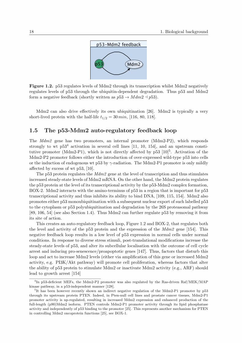
Figure 1.2. p53 regulates levels of Mdm2 through its transcription whilst Mdm2 negativelyregulates levels of p53 through the ubiquitin-dependent degradation. Thus p53 and Mdm2form a negative feedback (shortly written as p53→Mdm2 a p53).
Mdm2 can also drive effectively its own ubiquitination [26]. Mdm2 is typically a veryshort-lived protein with the half-life t1/2 = 30min, [116, 80, 118].
1.5 The p53-Mdm2 auto-regulatory feedback loop
The Mdm2 gene has two promoters, an internal promoter (Mdm2-P2), which respondsstrongly to wt p534 activation in several cell lines [11, 10, 154], and an upstream consti-tutive promoter (Mdm2-P1), which is not directly affected by p53 [10]5. Activation of theMdm2-P2 promoter follows either the introduction of over-expressed wild-type p53 into cellsor the induction of endogenous wt p53 by γ-radiation. The Mdm2-P1 promoter is only mildlyaffected by excess of wt p53, [10].
The p53 protein regulates the Mdm2 gene at the level of transcription and thus stimulatesincreased steady-state levels of Mdm2 mRNA. On the other hand, the Mdm2 protein regulatesthe p53 protein at the level of its transcriptional activity by the p53-Mdm2 complex formation,BOX-2. Mdm2 interacts with the amino-terminus of p53 in a region that is important for p53transcriptional activity and thus inhibits its ability to bind DNA, [109, 115, 154]. Mdm2 alsopromotes either p53 monoubiquitination with a subsequent nuclear export of such labelled p53to the cytoplasm or p53 polyubiquitination and degradation by the 26S proteasomal pathway[89, 106, 54] (see also Section 1.4). Thus Mdm2 can further regulate p53 by removing it fromits site of action.
This creates an auto-regulatory feedback loop, Figure 1.2 and BOX-2, that regulates boththe level and activity of the p53 protein and the expression of the Mdm2 gene [154]. Thisnegative feedback loop results in a low level of p53 expression in normal cells under normalconditions. In response to diverse stress stimuli, post-translational modifications increase thesteady-state levels of p53, and alter its subcellular localisation with the outcome of cell cyclearrest and inducing pro-senescence/proapoptotic genes [147]. Thus, factors that disturb thisloop and act to increase Mdm2 levels (either via amplification of this gene or increased Mdm2activity, e.g. PI3K/Akt pathway) will promote cell proliferation, whereas factors that alterthe ability of p53 protein to stimulate Mdm2 or inactivate Mdm2 activity (e.g., ARF) shouldlead to growth arrest [154]
4In p53-deficient MEFs, the Mdm2-P2 promoter was also regulated by the Ras-driven Raf/MEK/MAPkinase pathway, in a p53-independent manner [128].
5It has been however recently shown an indirect negative regulation of the Mdm2-P1 promoter by p53through its upstream protein PTEN. Indeed, in Pten-null cell lines and prostate cancer tissues, Mdm2-P1promoter activity is up-regulated, resulting in increased Mdm2 expression and enhanced production of thefull-length (p90)Mdm2 isoform. PTEN controls Mdm2-P1 promoter activity through its lipid phosphataseactivity and independently of p53 binding to the promoter [25]. This represents another mechanism for PTENin controlling Mdm2 oncoprotein functions [25], see BOX-1.
1.6. Wild-type p53-induced phosphatase 1, Wip1 19
Note that except for Mdm2-mediated degradation of p53, p53 may be targeted for degra-dation by other E3 ligases as well as by non-proteasomal mechanisms. However, Mdm2 isbelieved to be the major physiological antagonist of p53 [106]. In addition, no molar excessof Mdm2 over p53 is necessary for efficient p53 degradation: one molecule of Mdm2 may pro-mote degradation of several p53 molecules [61]. Interestingly, whilst Mdm2 binding to p53represents one inhibitory mechanism of p53 activity, stable p53-Mdm2 complexes were barelydetectable in several cell lines including DA-1 murine lymphoma, ML-1 myeloid leukaemiaand BALB/c-3T3 fibroblasts [61].
In addition to the p53-Mdm2 negative feedback, there are several other players which can(positively or negatively) contribute to the p53-Mdm2 loop. Currently there exist at least 7negative feedbacks regulating p53, most of them between p53 and Mdm2 (and other proteins)and several positive feedbacks (between p53 and PTEN, p14/19 ARF, Rb, Dapk1, c-Ha-Ras,DDR1, Rorα), [60, 69].
BOX-2: p53-Mdm2 auto-regulatory loop
Auto-regulatory feedback loop between p53 and Mdm2 consists in regulation:
• of Mdm2 by p53 at the transcriptional level (p53 is a transcription factorfor Mdm2 gene),
• of p53 by Mdm2 through either
– p53-Mdm2 complex formation and inhibition of p53 activity,
– promoting mono-ubiquitination and nuclear export of p53, or
– promoting poly-ubiquitination and degradation of p53 by the 26Sproteasomal pathway.
1.6 Wild-type p53-induced phosphatase 1, Wip1
The Wip1 gene was identified as a novel transcript whose expression was induced in responseto γ-IR in a p53-dependent manner in the Burkitt lymphoma (BL) cells. The BL cells carrya wt p53 gene, they can arrest a cell in the G1 checkpoint and induce apoptosis following IR,[52] and citations therein.
The Wip1 protein with the apparent molecular mass of 61 kDa is a member of the ser-ine/threonine protein phosphatase 2C (PP2C) family and was found exclusively in the nucleiof BL cells6. The levels of nuclear Wip1 increased with an apparent peak of its mRNA at2hr in a p53-dependent manner [52].
The Wip1 gene is amplified in several human cancers such as breast cancer, neuroblas-toma, and ovarian carcinomas, predominantly those that still retain wt p53 [92, 95]. Patientswith cancers which over-express Wip1 exhibited poorer prognosis than their counterpartswith normal Wip1 [92]. This indicates that Wip1 can function as an oncogene in these (andother) tumours. Inactivation of Wip1 resulted in the activation of p53 and/or ATM path-ways with a clear suppression of tumorigenesis in several murine models, [155] and citationstherein.
The protein Wip1 targets p53 as well as other proteins including ATM, Mdm2, Chk1,Nbs1 and HA2X for dephosphorylation, [136, 137, 155]. Thus it is considered as a major
6Wip1 is even found to be tightly bound to chromatin throughout the cell cycle and it was shown to interactwith H2AX (a marker of DSB) following γ-IR [95].

20 1. Biological background
homeostatic regulator of the DDR, mainly because of dephosphorylating proteins that aresubstrates ATM [92].
1.7 Dynamics of the proteins in cancer cells following DNAdamage
1.7.1 p53 dynamics measured over populations of cells
The levels of p53 in normal cells are regulated by the rapid turnover of the protein. Activationof the p53 pathway following DNA damage results in increased level of p53 mainly throughthe disruption of p53-Mdm2 interactions7.
Several cancer cell lines tolerate wt p53 (which would be normally growth-suppressive) ifthey over-express the Mdm2 (and/or Wip1) gene [27, 92]. For instance, the osteosarcoma cellline (OsA-CL) and the myeloid leukaemia cells (ML-1) both have wt p53 gene and amplifiedMdm2 gene. Exposure of these cells to γ-irradiation was associated with high levels of p53,which was active as a transcription factor for Mdm2. Figure 1.3 shows a time course ofchanges of p53 and Mdm2 in ML-1 cells after exposure to 2Gy of γ-irradiation. After DNAdamage, p53 increases rapidly and peaks at about 3hrs post-irradiation. Then the p53 levelsdecrease by 5hrs after damage. In contrast, Mdm2 protein levels are not detectably changedat 1hr post-irradiation (suggesting that Mdm2 induction is transcriptionally dependent onp53), noticeably increase at the 3hrs time point, peaks at 5hrs, and is decreasing by 9hrspost-irradiation. Notably, the level of Mdm2 peaks about 2 hours later than the level of p53following γ-IR, [27].
Figure 1.3. Induction of p53 and Mdm2 in ML-1 cells in response to IR of 2Gy. (A)Immunoblot for p53 and Mdm2 proteins in ML-1 cells (expressing wt p53). Topoisomerase I(Topo I) protein levels are shown as a control. (B) Densitometric quantitation of the relativechanges in the levels of p53 and Mdm2 proteins in ML-1 cells at various times after IR. Foroptimal display of changes over time, the levels were normalised so that the peaks of p53 andMdm2 expression were equal to 1. Relative changes of Mdm2 protein levels in HL-60 cells(which do not have p53 gene) at various times after IR are also shown. The figure taken from[27], copyright by the National Academy of Sciences.
7Nuclear accumulation of p53 may be partly achieved through its increased half-life. p53 is a short-livedprotein with t1/2 = 20 − 30min [116]; the half-life of wt p53 in human Saos-2 cells without any Mdm2 wasdetermined to 7.3 hours whilst the half-life of wt p53 in these cells with exogenous Mdm2 to 2.5 hours [74].

1.7. Dynamics of the proteins in cancer cells following DNA damage 21
Another and similar time course of p53 and Mdm2 levels from the murine lymphoma cells(DA-1), ML-1 cells, and BALB/c-3T3 fibroblasts when exposed to the dose of 2Gy of γ-IRwas observed in [61]. In case of DA-1 cells, p53 peaked at the 1hr and Mdm2 at 1.5− 2hrstime point post-irradiation. In ML-1, p53 peaked at 1hr at remained at the peak for 2 hoursthan it started to decay; Mdm2 peaked at 3 − 4hrs in ML-1, Figure 1.4. Similarly to theprevious case, maximal Mdm2 induction coincided with rapid p53 loss during recovery fromDNA damage. The levels of p53 mRNA remained fairly unchanged [61].
Figure 1.4. Immunoblots for p53 and Mdm2 induction in DA-1 (left panel) and ML-1 (rightpanel) cells in response to IR of 2Gy. α-tubulin levels are shown as a control. The figurestaken from [61]. Reprinted by permission from Macmillan Publishers Ltd: Letters to Nature[61], copyright 1997.
1.7.2 p53 oscillations in single cells
Experiments in individual living breast cancer cells showed that population-averaged analy-sis could lead to misinterpretation of actual dynamical responses of proteins. Indeed, usingmeasurements across a population of cells (in immunoblots) it was observed that p53 ex-hibits a series of damped oscillations following DNA damage [86], Figure 1.5. New methodsallowing high-resolution time-lapse imaging in individual living cells improved the previouslyobserved p53 dynamics from damped to sustained oscillations of fixed amplitude and periodsof oscillations [77, 56], Figure 1.6. Previously it was also observed that the levels of thephosphorylated ATM (ATM-P), when measured at high frequency during the first hour ofDDR, increase rapidly and reach maximal level within 5−15min after damage, then followedby a slow decrease [7]. However, when phosphorylated ATM was measured every hour for acertain period of time, a series of oscillations were identified after DNA damage, [15, 124].
The concentrations of p53 (and also Mdm2, Wip1, ATM) exhibit sustained oscillationswith the fixed amplitude and period (duration) of p53 pulses8 which may persist for severaldays. In the case of p53, periods of oscillations range from 4−7hrs in different cells. A numberof pulses can be also different from cell to cell and it depends on the dose of γ-irradiation ordrugs (e.g., NCS), meaning that the number of pulses increases with the increasing damagedose, [56]. On the other side, the amplitude and duration of p53 pulses in DDR (initiated by
8In fact, due to a stochasticity in the protein signalling, the amplitudes of oscillations vary widely frompeak to peak whilst the variation in periods is less significant [56], however, in average, oscillations are of fixedamplitude and duration [77].
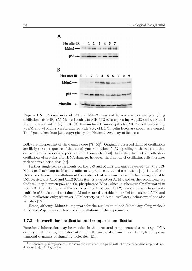
22 1. Biological background
Figure 1.5. Protein levels of p53 and Mdm2 measured by western blot analysis givingoscillations after IR. (A) Mouse fibroblasts NIH 3T3 cells expressing wt p53 and wt Mdm2were irradiated with 5Gy of IR. (B) Human breast cancer epithelial MCF-7 cells, expressingwt p53 and wt Mdm2 were irradiated with 5Gy of IR. Vinculin levels are shown as a control.The figure taken from [86], copyright by the National Academy of Sciences.
DSB) are independent of the damage dose [77, 56]9. Originally observed damped oscillationsare likely the consequence of the loss of synchronisation of p53 signalling in the cells and thuscancelling of pulses over a population of these cells, [124]. Note also that not all cells showoscillations of proteins after DNA damage; however, the fraction of oscillating cells increaseswith the irradiation dose [56].
Further single-cell experiments on the p53 and Mdm2 dynamics revealed that the p53-Mdm2 feedback loop itself is not sufficient to produce sustained oscillations [15]. Instead, thep53 pulses depend on oscillations of the proteins that sense and transmit the damage signal top53, particularly ATM and Chk2 (Chk2 itself is a target for ATM), and on the second negativefeedback loop between p53 and the phosphatase Wip1, which is schematically illustrated inFigure 3. Even the initial activation of p53 by ATM (and Chk2) is not sufficient to generatemultiple p53 pulses and sustained p53 pulses are detectable in parallel to sustained ATM andChk2 oscillations only; whenever ATM activity is inhibited, oscillatory behaviour of p53 alsovanishes [15].
Hence, although Mdm2 is important for the regulation of p53, Mdm2 signalling withoutATM and Wip1 does not lead to p53 oscillations in the experiments.
1.7.3 Intracellular localisation and compartmentalisation
Functional information may be encoded in the structural components of a cell (e.g., DNAor enzyme structures) but information in cells can be also transmitted through the spatio-temporal dynamics of signalling molecules [124].
9In contrast, p53 response to UV shows one sustained p53 pulse with the dose-dependent amplitude andduration [14], c.f., Figure 6.9.

1.7. Dynamics of the proteins in cancer cells following DNA damage 23
Figure 1.6. Oscillations of p53 and Mdm2 in a single cell: time-lapse imaging of the p53and Mdm2 proteins fused with CFP (in green) and YFP (in red), respectively, in a singlecell following DNA damage caused DSB. The levels of the proteins are normalised. Creditsto the Uri Alon Lab [2].
The wt p53 protein, as a transcription factor, is largely nuclear when it is in the acti-vated mode, but a certain fraction of p53 plays a part outside the nucleus [106], notablyas a transcription-independent factor involved in the induction of apoptosis [59, 111]. Thecytoplasmic clearance of p53 may lead to autophagy [59]. There are three nuclear localisationsignals (NLS) at p53 and a couple of nuclear export signals (NES) and thus p53 is in principleable to shuttle between nucleus and cytoplasm through direct interaction with the nuclearimport and nuclear export machineries [138]. Nonetheless, Mdm2 seems to be a dominantregulator of subcellular localisation of p53, likely because of the rapid clearance of p53 fromthe DNA sites [106, 42]. In addition, localisation of p53 is dependent on its oligomeric status[139] and except for Mdm2 there are other cellular substrates which can affect p53 location,see [111].
ATM is also predominantly concentrated in the nucleus with only 10-20% of its moleculesfound in the cytoplasm, particularly bound to peroxysomes and endosomes [81]. Fluorescentmicroscopy techniques have confirmed this spatial distribution of ATM between the nucleusand the cytoplasm. However, only the nuclear fraction of ATM is autophosphorylated inresponse to DNA damage induced by ionising radiation, and activated ATM proteins formdetectable foci that are colocalised with the foci of γ-H2AX, a marker of DNA DSB. Cyto-plasmic ATM can neither autophosphorylate itself nor phosphorylate its substrates [159].
The transcription and translation of the Mdm2 and Wip1 genes are localised to thenucleus and cytoplasm, respectively, [146]. Both their protein products Mdm2 and Wip1are also observed to accumulate mainly in the nucleus in the DDR initiated by ionisingradiation [5, 52, 116].

24 1. Biological background

2
Conceptual and MathematicalFoundations
Bearing biological aspects in mind, we can proceed with modelling p53 protein net-work in a single cell. Motivated by the experiments, a model for p53 activation inresponse to DNA DSB should involve information-transmitting signal, ATM, whichis able to sense the presence of DSB and deliver it to p53, and homeostatic regula-tors of the DNA damage response, Wip1 and Mdm2. The protein p53 is naturallyinvolved in the modelling. This chapter presents basic concepts for modelling p53protein network; mathematical principles and main hypotheses used in modelling arestated.
Organisation of the chapter is as follows: Section 2.1 introduces enzyme reactionsalthough these reactions are studied more deeply in Chapter 8. Expression and regu-lation of Wip1 and Mdm2 through rather simple gene regulatory networks (GRN) aswell as induction and regulation of ATM and p53 is discussed in Section 2.2. Sec-tions 2.3 and 2.4 then focus on the intracellular movement of species in the nuclearand cytoplasmic compartments and their translocation between the compartmentsthrough the nuclear membrane. Obviously, these two section apply mainly to PDEmodels due to the spatial representation of the problem. A review of the existingmathematical models is given at the end of this chapter in Section 2.5.
2.1 Protein-protein interactions; post-translational modifica-tions
Cellular responses are controlled either by one particular functionally active protein or byseveral proteins whose activation and activity towards other proteins in highly specific situ-ations depend on other factors and conditions to which cells are exposed. On the molecularbasis, roles of proteins in specific networks are influenced by protein-protein interactionseither through post-translational modifications (by attaching a phosphate or acetyl group,ubiquitin to a protein, etc.) or by various compounds formation. For example, stabilisa-tion of p53 through escape from proteasome degradation, which is the major mechanism forregulating p53 protein level, is achieved mainly via post-translational mechanism.
Post-translational modifications (e.g., protein-protein interactions) can be advantageouslyrepresented as enzyme reactions (EnR). The prototypic enzyme reaction is schematically
25
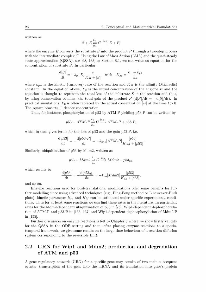
26 2. Conceptual and Mathematical Foundations
written as
S + Ek+
k−C
kp+−→ E + P,
where the enzyme E converts the substrate S into the product P through a two-step processwith the intermediate complex C. Using the Law of Mass Action (LMA) and the quasi-steadystate approximation (QSSA), see [68, 133] or Section 8.1, we can write an equation for theconcentration of substrate S. In particular,
d[S]
dt= −kp+E0
s
KM + [S]with KM =
k− + kp+k+
where kp+ is the kinetic (turnover) rate of the reaction and KM is the affinity (Michaelis)constant. In the equation above, E0 is the initial concentration of the enzyme E and theequation is thought to represent the total loss of the substrate S in the reaction and thus,by using conservation of mass, the total gain of the product P (d[P ]/dt = −d[S]/dt). Inpractical simulations, E0 is often replaced by the actual concentration [E] at the time t > 0.The square brackets [·] denote concentration.
Thus, for instance, phosphorylation of p53 by ATM-P yielding p53-P can be written by
p53 +ATM -Pk+
k−C
kph1−→ ATM -P + p53-P,
which in turn gives terms for the loss of p53 and the gain p53-P, i.e.
d[p53]
dt= −d[p53-P ]
dt= −kph1[ATM -P ]
[p53]
Kph1 + [p53].
Similarly, ubiquitination of p53 by Mdm2, written as
p53 +Mdm2k+
k−C
kub−→Mdm2 + p53ub,
which results tod[p53]
dt= −d[p53ub]
dt= −kub[Mdm2]
[p53]
Kub + [p53],
and so on.Enzyme reactions used for post-translational modifications offer some benefits for fur-
ther modelling since using advanced techniques (e.g., Ping-Pong method or Lineweaver-Burkplots), kinetic parameter kp+ and KM can be estimated under specific experimental condi-tions. Thus for at least some reactions we can find these rates in the literature. In particular,rates for the Mdm2-dependent ubiquitination of p53 in [78], Wip1-dependent dephosphoryla-tion of ATM-P and p53-P in [136, 137] and Wip1-dependent dephosphorylation of Mdm2-Pin [155].
Further discussion on enzyme reactions is left to Chapter 8 where we show firstly validityfor the QSSA in the ODE setting and then, after placing enzyme reactions to a spatio-temporal framework, we give some results on the large-time behaviour of a reaction-diffusionsystem corresponding to the reversible EnR.
2.2 GRN for Wip1 and Mdm2; production and degradationof ATM and p53
A gene regulatory network (GRN) for a specific gene may consist of two main subsequentevents: transcription of the gene into the mRNA and its translation into gene’s protein

2.2. GRN for Wip1 and Mdm2; production and degradation of ATM and p53 27
product. From a modelling point of view, we can write two equations for the mRNA and theprotein P ,
d[mRNA]
dt= I − δmRNA[mRNA],
d[P ]
dt= k[mRNA]− δP [P ],
(2.1)
where δmRNA and δP are degradation rates for mRNA and P , respectively; k is a translationrate; and I is a source term for the mRNA production, which usually depends on the specificproperties of the protein network.
For example, in Goodwin’s “protein-mRNA” model [57], the expression of a single geneis controlled by its protein product P (thus, closing the negative feedback loop). In this case
I =a1
A1 + k1[P ],
where a1, A1 and k1 are some constants.
Another example of the source I, which is also applied here for the transcription of Mdm2and Wip1 genes, involves Hill’s kinetics (i.e. Hill function of coefficient n). In particular,
I = kS[TF ]n
KnS + [TF ]n︸ ︷︷ ︸
TF-dependent mRNA production
+ kC︸︷︷︸TF-independent mRNA production
where the first term is the Hill function modelling transcription activity of a transcriptionfactor TF. The protein p53 preferentially forms tetramers, binds DNA and transcriptionallyacts as a tetramer [53, 66, 152]. Hence, p53-dependent transcription is modelled by choosingn = 4, since we adopt a generally accepted principle according to which n is equal to thenumber of binding sites of a transcription factor [152], see also [68] Chap. 1. In addition,at least Mdm2 has also a p53-independent promoter. Therefore, we consider a constantbasal p53-independent production rate kC for Mdm2 mRNA. It is not clear if Wip1 hasanother p53-independent promoter. Nevertheless, we consider a basal production rate forWip1 mRNA as well. The parameters kS and KS are chosen so that p53 is the dominant TFfor these genes and the levels of Mdm2 and Wip1 are proportional to the level of p53.
The mRNAs of Mdm2 and Wip1 (likely bound to another proteins acting as their “chap-erones”, mRNP) then move from the transcription sites in the nucleus to the cytoplasmwhere they are translated. We assume that translation of mRNAs into proteins occurs inthe cytoplasm only and, following [1, 142], we adopt the hypothesis saying that the proteinssynthesised outside of the endoplasmic reticulum (ER) move to the nucleus whereas the pro-teins produced in the ER associate likely with the structures in the cytoplasm. Translationis modelled as a linear contribution to the overall protein concentrations. The translationrate is usually independent of the coding sequence, and thus it is (more or less) similar for allproteins in a given cell type at given conditions [16]. Thus we assume that translation ratesfor Mdm2 and Wip1 are equal to each other (i.e., ktm = ktw).
The mRNA is degraded by a ribonuclease which competes with ribosomes to bind tomRNA. Roughly speaking, if a ribosome binds to mRNA, it will be translated, if a ribonu-clease does, it will be degraded. Most eukaryotic mRNAs have half-lives less than 30 minutesand the most short-lived are those that encode proteins whose concentrations need to changerapidly based on the cellular context, such as transcription regulators [1]. Proteins are de-graded by a complex cellular machinery, including the 26S proteasome which targets speciestagged by ubiquitin (e.g., p53 but also Mdm2, Bax, p21 and other proteins [26]). Degradation

28 2. Conceptual and Mathematical Foundations
substrate t1/2 [h] δ [h−1] source
p53 (with wt Mdm2) 1/3 2 [116]
p53 (without wt Mdm2) 7 0.1 [74]
p53 mRNA 1/3 2 [1]
Mdm2 mRNA 1 0.7 [104]
Wip1 mRNA? – 0.7 –
Mdm2 0.5 1.38 [116, 118, 154]
Wip1? – 1.38 –
Table 2.1. The half-lives t1/2 and degradation terms δ of the species used in the models;?the half-lives of the Wip1 and its mRNA are not known, however, since it is short-livedprotein as p53 and Mdm2 [26], we assume the same degradation terms as for Mdm2 and itsmRNA.
depends on the oligomeric status (the monomer and multimers may be degraded at differentrates).
The rate of degradation δ for species (proteins, mRNAs) as above can be deduced from asimple formula giving into relation the first-order (degradation) rate and the half-life t1/2 ofthe species (usually a measurable quantity):
t1/2 =log 2
δ. (2.2)
The half-life t1/2 is the amount of time which is necessary for a species of a certain concen-tration to fall to half its value as measured at the beginning of the time period [105], p. 457.Table 2.1 summarises publicly available half-lives and the corresponding degradation ratesfor all the species1.
Activation of ATM and its specific regulation following DNA damage as well as productionand degradation of p53 are left to separate sections.
2.2.1 ATM activation in response to DSB
Specific regulation of ATM, explained in Section 1.3, allows us to exclude its synthesis fromour considerations. The observed way of ATM regulation through its ability to switch be-tween active monomeric and inactive dimeric states, keeping thus ATM in overall constantconcentration, can be used rather than introducing another variable for ATM mRNA2. Inresponse to DSB, ATM dimers dissociates into active monomers either by sensing changes inheterochromatin (as deduced from in vivo experiments) or through interaction with the MRNcomplex (as observed in in vitro experiments). Whether ATM is activated adjacent to or ata distance from the DNA, its activation is observed to be very fast, and we represent ATMmonomerisation and activation as an enzymatic reaction initiated by an unknown signal E,
1Short half-lives of the species (< 1hr) strengthen the hypothesis that species that need to be changedpromptly in their concentration, including regulators of the cell cycle and several transcription factors such asp53 are degraded rapidly mainly by ubiquitin-dependent proteolysis, [106, 26] and citations therein.
2Although we could not find any evidence in the literature, we assume that ATM is long-lived protein withthe half-life of several hours; thus, we suppose that the degraded ATM molecules are continuously replaced bynew ones so that the total concentration of ATM remains fairly constant. Since ATM is 370 kDa large proteinwe can speculate that its inactivation through the dimerisation instead of degradation is energetically moreprofitable.

2.2. GRN for Wip1 and Mdm2; production and degradation of ATM and p53 29
Figure 2.1. A schematic representation of ATM activation by a DNA-damage-transmittingsubstrate (although hypothetical) E and its deactivation by Wip1.
assumed to be a hypothetical molecule (E can be the MRN complex or any other protein;hereafter expressed in µM), Figure 2.1.
Taking all this together, we can represent ATM dimer dissociation and ATM activation(for simplicity these two events are assumed to occur simultaneously) by the reaction
ATM -D + E Complexkph2−→ E + 2ATM -P,
c.f. (3.2) below, where ATM-D denotes dimeric ATM and ATM-P denotes phosphorylatedactive monomer. On the other site, ATM deactivation by Wip1 and subsequent dimerisationcan be modelled (similarly as a simultaneous process) by
Wip1 + 2ATM -P Complexkdph2−→ ATM -D +Wip1,
c.f. (3.3) below. Application of the Law of Mass Action and QSSA3, yields reaction termsfor ATM-P and ATM-D losses and gains, respectively,
d[ATM -D]
dt= −kph2E
[ATM -D]
Kph2 + [ATM -D]+ kdph2[Wip1]
[ATM -P ]2
Kdph2 + [ATM -P ]2,
d[ATM -P ]
dt= 2kph2E
[ATM -D]
Kph2 + [ATM -D]︸ ︷︷ ︸ATM-P activation
− 2kdph2[Wip1][ATM -P ]2
Kdph2 + [ATM -P ]2︸ ︷︷ ︸Wip1-depedent dephosphorylation of ATM-P
,(2.3)
c.f. (3.4), which can be further merged, just by recalling the conservation of ATM molecules4,into one equation for ATM-P,
d[ATM -P ]
dt=2kph2E
1
2(ATMTOT − [ATM -P ])
Kph2 +1
2(ATMTOT − [ATM -P ])
− 2kdph2[Wip1][ATM -P ]2
Kdph2 + [ATM -P ]2,
(2.4)
c.f. (3.12), which is the equation used in the ODE model. The single equation (2.4) forATM-P above cannot be generally used in PDE models where the motion of ATM-P and
3Application of the LMA and QSSA and thus these equations are precisely derived in Section 3.2.1.4ATM is conserved, i.e., [ATM -P ] + 2[ATM -D] = const over the time by our assumption on the constant
concentration of ATM.
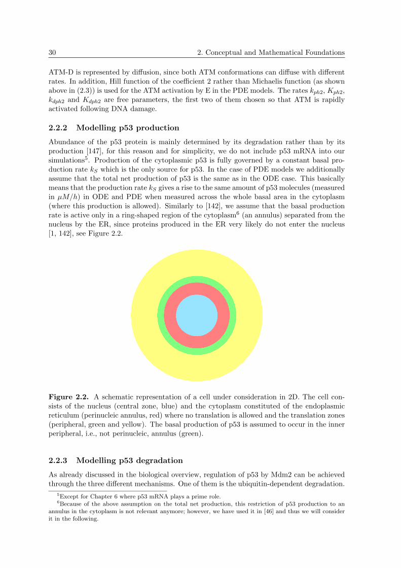
30 2. Conceptual and Mathematical Foundations
ATM-D is represented by diffusion, since both ATM conformations can diffuse with differentrates. In addition, Hill function of the coefficient 2 rather than Michaelis function (as shownabove in (2.3)) is used for the ATM activation by E in the PDE models. The rates kph2, Kph2,kdph2 and Kdph2 are free parameters, the first two of them chosen so that ATM is rapidlyactivated following DNA damage.
2.2.2 Modelling p53 production
Abundance of the p53 protein is mainly determined by its degradation rather than by itsproduction [147], for this reason and for simplicity, we do not include p53 mRNA into oursimulations5. Production of the cytoplasmic p53 is fully governed by a constant basal pro-duction rate kS which is the only source for p53. In the case of PDE models we additionallyassume that the total net production of p53 is the same as in the ODE case. This basicallymeans that the production rate kS gives a rise to the same amount of p53 molecules (measuredin µM/h) in ODE and PDE when measured across the whole basal area in the cytoplasm(where this production is allowed). Similarly to [142], we assume that the basal productionrate is active only in a ring-shaped region of the cytoplasm6 (an annulus) separated from thenucleus by the ER, since proteins produced in the ER very likely do not enter the nucleus[1, 142], see Figure 2.2.
Figure 2.2. A schematic representation of a cell under consideration in 2D. The cell con-sists of the nucleus (central zone, blue) and the cytoplasm constituted of the endoplasmicreticulum (perinucleic annulus, red) where no translation is allowed and the translation zones(peripheral, green and yellow). The basal production of p53 is assumed to occur in the innerperipheral, i.e., not perinucleic, annulus (green).
2.2.3 Modelling p53 degradation
As already discussed in the biological overview, regulation of p53 by Mdm2 can be achievedthrough the three different mechanisms. One of them is the ubiquitin-dependent degradation.
5Except for Chapter 6 where p53 mRNA plays a prime role.6Because of the above assumption on the total net production, this restriction of p53 production to an
annulus in the cytoplasm is not relevant anymore; however, we have used it in [46] and thus we will considerit in the following.

2.3. Diffusion of species in the cell 31
Once p53 is sufficiently ubiquitinated, the p53 protein is exported to the cytoplasm anddegraded by the 26S proteasome. Mdm2 plays a crucial role in the p53 ubiquitination asit attaches the first ubiquitin to p53. The effective p53 degradation however requires p53to be polyubiquitinated. Nonetheless, we assume that the sole ubiquitination by Mdm2 issufficient for p53 nuclear export and degradation for either degradation or nuclear export ofp53. We do not include actions of any other proteins that can either cooperate with Mdm2in the ubiquitination process (e.g., p300) or deubiquitinate p53 (e.g., Hausp). In addition,we do not assume any p53-Mdm2 complex formation since in some cancer cell lines (e.g.,DA-1, ML-1 and BALB/c-3T3 cells) these complexes were barely detectable [61]. Thus theMdm2-dependent degradation of p53, modelled as an enzyme reaction, yields
d[p53]
dt= − kub[Mdm2]
[p53]
Kub + [p53]︸ ︷︷ ︸ubiquitination of p53 by Mdm2
− δp53[p53].︸ ︷︷ ︸natural degradation
Note that, although Mdm2 is the main regulator of p53 (responsible for its nuclear clearance)we assume some natural Mdm2-independent degradation rates for the cytoplasmic p53 (withthe half-life of 7hrs and the corresponding δp53 = 0.1h−1, see Table 2.1). The rates for theMdm2-dependent degradation kub = 5min−1 and Kub = 1µM are taken from [78].
Stabilisation of p53 in the nucleus depends directly on its phosphorylation by ATM. Thuswe assume that the phosphorylated p53-P cannot be degraded by Mdm2.
2.3 Diffusion of species in the cell
Recent photobleaching techniques enable to track the fusion of a protein with the green flu-orescent protein (GFP) and thus measure diffusion of such fused proteins. Hinow et al. [64]estimate the nuclear diffusion of p53 fused with GFP in H1299 human large cell lung carci-noma cell to be ∼900 µm2/min, slower than the diffusion of GFP itself (∼2500 µm2/min),likely due to multimer formation.
We can assume that an individual p53 monomer migrates faster with a higher diffusivitythan the measured p53-GFP diffusivity. Hence, we will use the diffusion coefficient for p53equal to 1000 µm2/min as an average whether it migrates as a monomer, or multimer (how-ever, it cannot be exported through the nuclear membrane as a tetramer [138]). We are alsoaware of the fact that diffusion can be different in time and space due to many physical ob-stacles occurring in the cell or because of specific conditions to which the cell is exposed. Forinstance, the diffusion coefficient of p53-GFP reduced significantly after the drug treatmentby cisplatin and etoposide in HeLa cells: both drugs induce p53 activation and accumulationin the nucleus with diffusion 900 µm2/min decreased up to 200 µm2/min measured 16 hoursafter anticancer drug activity, [65].
Due to the lack of experimentally measured data, we set the values of the diffusion coef-ficients for the other proteins by comparing their molecular weights. We will use diffusionsof 1000µm2/min for Mdm2 and Wip1 (90 and 61 kDa, respectively, comparing to 53 kDa ofmonomeric p53) and 300µm2/min for ATM (370kDa) (monomeric or dimeric).
An increasing number of studies indicate that eukaryotic mRNAs form large ribonucleo-protein particles (mRNP) that are transported from the sites of transcription to the nuclearpores by random Brownian motion [20, 146]. Diffusion of an average mRNA-protein complexvary in the range 1.2 − 2.4µm2/min [20] and we will use the reference value for an aver-age as well as Mdm2 and Wip1 mRNP complexes equal to 1.8µm2/min. When comparedwith the diffusion of proteins, the diffusivities for the mRNP are smaller of several orders inmagnitude, however, note that mRNP complexes can be of weight as large as 1600 kDa [34].

32 2. Conceptual and Mathematical Foundations
Figure 2.3. Passive transport throughout the nuclear membrane: initial concentrations C0
and C0δ of a specie in two compartments divided by a membrane of the thickness δ. Due to
interaction of the species with the membrane, the actual concentrations outside of the bothsides of the membrane are C? and C?δ and inside of the membrane φ? and φ?δ . These valuesare generally different and satisfy φ? = HC? and φ?δ = HC?δ where H is a characteristicparameter dependent on interaction of the species with the membrane. For the flux J , Fick’s
first law then implies J = −Ddφ
dy≈ −D
φ?δ − φ?
δ= −DH
δ(C0
δ − C0), where D is a diffusion
rate of a transported substrate through the membrane and the difference of concentrationsC0δ − C0 is the driving force for the exchange of the substrate. The coefficient p = DH/δ
is the permeability rate (measured in µm/s) and it is the property of membrane. For moredetails see [112], p. 8–9. Figure taken from [112], copyright by Elsevier.
Due to similar nuclear and cytoplasmic cytosol viscosity we will consider the same diffusionvalues for both compartments. Note that there are other possibilities how to approximatediffusion coefficients of proteins, for example, by using Einstein’s formula [23] which, however,requires Stokes radii of the proteins, which are often not known.
2.4 Nucleocytoplasmic transmission, permeability
All the proteins under consideration have weights over 40 kDa (Table 5.2) so that theycan use active transport only (and not passive transport) for their translocation betweenthe two compartments. Similarly, mRNA–protein complexes (mRNPs), formed shortly aftermRNA synthesis at the transcription site, released to the nucleoplasm and moving towardthe nuclear membrane [146] usually have weights over 40 kDa7. However, comparing timescales of cargo translocations occurring within a period measured in seconds, a few minutesat most [127], and intracellular protein(mRNA)-dependent events which may hold over hours(e.g., accumulation of species in a compartment, regulation and degradation of the species inthe compartments, [56, 77]), we will not involve active transport mechanism here and thuskeep the model as simple as possible.
Instead, the transmission of a chemical is represented in our models by a diffusive fluxthrough the boundary that is proportional to the difference between the nuclear and the
7The protein in the mRNP usually assists in the mRNA export to the cytoplasm [32], see [32] for thedetailed description of mRNP translocation through the nuclear membrane.

2.5. Overview of other p53 models 33
cytoplasmic concentrations of the chemical, see Figure 2.3, i.e. we recall the so-called Kedem–Katchalsky boundary conditions (BC) as they have been suggested in [23] and already appliedin [43]. The same boundary conditions can be derived from the Fick’s first law for stationaryfluids (under the assumptions of no net movement, no bulk motion and no coupling effect ofmore cargoes transported simultaneously), see the caption in Figure 2.3. Additional remarksand the specific BC used in the PDE model are in Section 5.2.4.
Passive transport of the species through the nuclear membrane is determined by thediffusion and the permeability coefficient (itself dependent on the diffusion), see the captionof Fig. 2.3. Note that mRNA export from the nucleus to the cytoplasm can take 10–30minutes depending on the mRNA [16] which is likely caused not only by a relatively smalldiffusion but also a highly complex mRNA translocation through the nuclear envelope [32].This induces another delay in the response to transcriptional activation, since the mRNAcan be translated into a protein only once it is exported from the nucleus and binds to theribosomes.
ATM is assumed to be strictly nuclear, thus we assume that p53 phosphorylation byATM can occur only in the nucleus. Although Mdm2 is reported to be nuclear we assumethat it can freely migrate between the compartments in the ODE model (but not in thePDE models where it is assumed to move from the translation site in the cytoplasm to thenucleus) and it also can ubiquitinate unphosphorylated p53 in both compartments. Unlikep53-P, which is assumed to be localised to the nucleus only, p53 can freely migrate betweenthe compartments. The phosphatase Wip1 is assumed to move from the cytoplasm to thenucleus only since it is predominantly found to be the nuclear protein.
All the diffusion and permeability coefficients considered in our PDE simulations are listedin Table 5.2.
2.5 Overview of other p53 models
There are several mathematical models describing the p53-Mdm2 dynamics, for example thealready mentioned model by Lev Bar-Or et al. [86] which shows (numerically and experi-mentally) the presence of damped oscillations. The model developed by Batchelor et al. [15],which is actually based on the former models of Geva-Zatorsky et al. [56], includes nuclearconcentrations of the proteins, more or less, of all four species as we do, i.e. a signal (in-cluding ATM) that initiates p53 signalling and an inhibitor (including Wip1) that inhibitsp53. The models [15, 56] rely on Delayed Differential Equations (DDE). However, DDE mod-els may generate artificial rhythms in systems, which do not appear naturally, see [69] andreferences therein, so that the biological significance of the introduced delays in modellingprotein networks is most often far from obvious in those DDE models. Avoiding DDEs, theauthors in [69] convert the DDE system [15] into a system of ODEs. However, they still needto involve a positive feedback to obtain oscillations (they chose a recently observed positivefeedback involving Rorα).
Ma et al. [94, 151] also use DDE to simulate particular delays in representing the tran-scription of Mdm2 mRNA and translation of the mRNA into Mdm2. Their models containp53 activation by ATM kinase and nuclear species are considered only.
Ciliberto et al. [28] studies the negative feedback p53→Mdm2 a p53 supplemented by asimplified positive feedback to reconstruct p53-Mdm2 oscillations. In the positive feedback,p53 initiates activation of a cascade of protein interactions (involving PTEN, PIP2, PIP3and Akt) leading to a temporal inhibition of cytoplasmic Mdm2 translocation to the nucleus.T. Zhang et al. [160] explore the mechanism of p53-Mdm2 network of [28] and offer threeother models simulating p53-Mdm2 dynamics which combine different positive feedbacks with
34 2. Conceptual and Mathematical Foundations
the p53-Mdm2 negative feedback. As we have already mentioned there exist several positivefeedbacks between p53 and, e.g., PTEN, p14/19 ARF, Rb, Dapk1, c-Ha-Ras, DDR1 andRorα which could be in principle combined with the p53-Mdm2 negative feedback loop andgive a rise to oscillations8. In addition, the model in [160] proposes a mechanism enablinga cell to decide between cell cycle arrest and apoptosis, assuming that persistent p53 pulsestrigger apoptosis. X.P. Zhang et al. [161] combine results of [28, 160] and develop a two-phase switch model, which includes p53-Mdm2, ATM-p53-Wip1 and p53-PTEN-Akt-Mdm2feedback loops to simulate irreversible transition from cell cycle arrest to apoptosis9.
Both ODE models of [160, 161] simulate cell fate decision by involving transcription ofproarrest and proapoptotic proteins p21 and p53DINP1, respectively, the activation of which,however, is regulated by the p53 affinity for the genes. Following this affinity assumption,proarrest proteins are produced initially in an early cell response phase to DSB (controlledby a “p53-arrester”) and proapoptotic proteins are produced later after a few p53 pulses(controlled by a “p53-killer”)10.
The p53-dependent transcriptional regulation of proteins is modelled by using Hill func-tions, mostly with coefficients 3 and 4, in the mentioned works [28, 94, 151, 160, 161].
Another model which simulates p53 signalling network through the p53-Mdm2 negativefeedback combined with PTEN/Akt positive feedback and taking stochastic effects into ac-count is proposed by Puszynski et al. [126]. In their recent work [125] (based on [126])they explore pharmacodynamics of a small molecule Nutlin-3 which is able to inhibit p53-Mdm2 interactions. Sturrock et al. [141, 142, 143] and Dimitrio et al. [42, 43] study the solep53-Mdm2 negative feedback (without active roles of ATM and Wip1) in maintaining p53oscillatory dynamics using spatial PDE models.
8This confirms the complexity of p53 signalling in the sense that whenever one path of the p53 network isinactivated for some reason, the proper oscillatory behaviour of p53 can be still triggered by another one ormore paths which can contribute to the normal p53 signalling, etc..
9A tricky part of the models using Akt/PTEN signalling is in an uncertainty in the experimental results,see BOX-1.
10However, as it is discussed in the biological review, such affinity-based preference of p53 for the downstreamsubstrates was not shown in several studies.

3
Physiological and compartmentalODE model for the p53 network
We start our modelling with a physiological and compartmental ODE model whichis an extension of the model of L. Dimitrio et al. [43, 42]. Unlike in the originallyproposed model, we integrate ATM and Wip1 into the p53-Mdm2 dynamics so thatp53 activation and regulation can be modelled more plausibly with respect to the rele-vant biological observations discussed in the biological overview. Thus, in contrast tothe model in [43, 42], which took into account the sole p53-Mdm2 negative feedbackonly, we consider all four species including ATM activating the DDR in response toDSB and Wip1 acting to maintain homeostasis in the DDR.
Organisation of the chapter is as follows: A short introduction to ODE modellingfor p53 is in Section 3.1. Section 3.2 which presents the ODE model is then followedby numerical simulations in Section 3.3 and concluding remarks in Section 3.4.
Results presented in this chapter were published in [47],
[47] J. Elias, L. Dimitrio, J. Clairambault, and R. Natalini. The p53 protein andits molecular network: Modelling a missing link between DNA damage and cellfate. Biochimica et Biophysica Acta (BBA) - Proteins and Proteomics, 1844(1,Part B):232–247, 2014.
3.1 Introduction to the ODE model
Most of the existing models describing p53 activation and regulation in single cells followingtheir exposure to DNA damaging stress agents rely on either DDEs or ODEs modelling thep53-Mdm2 negative feedback alone or in combination with a positive feedback. We showthat p53 oscillations that have been observed in individual cells can be reconstructed andpredicted by compartmentalising cellular events occurring after DNA damage, either in thenucleus or in the cytoplasm, and by describing network interactions, using ODEs, betweenthe ATM, p53, Mdm2 and Wip1 proteins, in each compartment, nucleus or cytoplasm, andbetween the two compartments.
The compartmental p53-Mdm2 model developed by L. Dimitrio et al. [42, 43] is extendedby considering the ATM and Wip1 proteins, since in the light of new evidence from single cellexperiments, the p53-Mdm2 negative feedback should not be sufficient for triggering oscilla-
35
36 3. Physiological and compartmental ODE model for the p53 network
tions. Instead, initiation and regulation of p53 must involve the ATM and Wip1 proteins, thedynamics of which should be fully described by mathematical variables, solutions of ODEs,rather than represented by constant parameters. As previously discussed, ATM is interpretedas an identifier of DNA DSB, although it is not a direct DNA DSB sensor [117]. In our con-text, a special signal denoted by E acts as a transmitter of information about the presence ofDNA DSBs, and it is assumed to be a constant positively correlated with the DNA damagedose1. In the original model, compartmentalisation of cellular events together with the p53-Mdm2 feedback (p53→ Mdm2 a 53) led to the desired p53 oscillatory behaviour even witha constant ATM (considered as a measure of DNA damage). Under our new assumptions,ATM and Wip1 concentration are considered as continuous time-dependent functions, andwe show that the feedbacks p53→Mdm2 a p53 and ATM → p53→Wip1 a ATM togetherwith compartmental distribution of proteins can then reconstruct the oscillatory dynamics ofthese proteins.
3.2 ATM-p53-Mdm2-Wip1 compartmental model
In this section, we design and analyse a mathematical model that can successfully be used toreconstruct in silico experimentally observed dynamics of proteins, namely, the main cellularactor p53, ATM as a protein transferring the DNA damage signal, Wip1 as a dephospho-rylation factor of both p53 and ATM, and Mdm2 that tags p53 for degradation. Note thatour model is compartmental in the sense that we strictly distinguish the activities of proteinsoccurring in the nucleus from those occurring in the cytoplasm, as it is shown on Figure 3.1.
3.2.1 Modelling ATM activation and deactivation
ATM activation, i.e. its autophosphorylation and consequent dissociation of ATM dimersinto (active) monomers, can be modelled in several ways. The simplest way is through thedissociation reaction
ATM -Dkmk−m
ATM -P +ATM -P, (3.1)
where ATM-D denotes a compound of two ATM kinases and ATM-P is active (phosphory-lated) ATM. In our model, ATM in inactivate state is considered in the form of dimers only.The constants km and k−m denote, respectively, the monomerisation (forward) and dimerisa-tion (reverse) rates of the reaction. Reaction (3.1) involves monomerisation (dissociation) ofa dimer complex ATM-D to the two active ATM species with the rate km and dimerisationof two ATM-P monomers to produce ATM-D with the rate k−m. The Law of Mass Actionthen can give mathematical relations between ATM-D and ATM-P, with the production ofATM-D being equal to the half degradation of ATM-P [68]. A disadvantage of presenting theactivation/deactivation of ATM as in (3.1), however, is that it does not mention any signalinitiating ATM-D dissociation, whereas such a signal is thought to be produced by changesin the chromatin structures after DNA damage [7] and/or by the MRN complex as a DNAstrand breaks sensor [117].
Hence, a more convenient way to represent ATM activation with the perspective of fur-ther analysis is to involve a hypothetical, likely molecular and so far biologically (in vivo)unidentified DNA damage signal E, produced by DNA damage recognition sensors, transmit-ted to and sensed by ATM, resulting in the dissociation of ATM dimers into two molecules
1We assume that the higher doses a cell is exposed to, the bigger number of DSB is caused, the strongeractivation signal E is produced.

3.2. ATM-p53-Mdm2-Wip1 compartmental model 37
of ATM-P, i.e.
ATM -D + Ekik−i
Complexkph2−→ E + 2ATM -P (3.2)
with the corresponding kinetic rates ki, k−i and kph2. This reaction is not a typical enzymaticreaction since the enzyme-like signal E in this approach is a non-specified signal correspondingto DNA damage; it is not necessarily an enzyme; however, we assume that E is not amplified,reduced nor changed otherwise in a short time interval.
ATM deactivation by Wip1 is modelled similarly as
Wip1 + 2ATM -Pkjk−j
Complexkdph2−→ ATM -D +Wip1. (3.3)
Here, it is assumed that phosphatase Wip1 exists in a sufficient concentration to dephos-phorylate ATM active monomers in the sense that whenever one ATM-P protein is dephos-phorylated, another dephosphorylated ATM protein is present, so that they are immediatelybound to the dimeric ATM-D. Kinetic rates are denoted by kj , k−j and kdph2.
Note that ATM activation and deactivation by Wip1 occur in the nucleus.The Law of Mass Action (LMA) and the QSSA [68, 133] then yield differential equations
for (3.2) and (3.3); in particular, changes of concentrations in time of ATM-D and ATM-Pare, respectively,
d[ATM -D]
dt= −kph2E
[ATM -D]
Kph2 + [ATM -D]+ kdph2[Wip1]
[ATM -P ]2
Kdph2 + [ATM -P ]2,
d[ATM -P ]
dt= 2kph2E
[ATM -D]
Kph2 + [ATM -D]− 2kdph2[Wip1]
[ATM -P ]2
Kdph2 + [ATM -P ]2,
(3.4)
since the rate of change of ATM-D is half that of ATM-P. Here Kph2 =k−i + kph2
kiand
Kdph2 =k−j + kdph2
kjare the Michaelis rates of reactions (3.2) and (3.3), and kph2 and kdph2
are the velocities of these reactions.Indeed, using the Law of Mass Action and the QSSA, the loss of ATM-D derived from
the first reaction (3.2) can be written in the form
d[ATM -D]
dt= −kph2E
[ATM -D]
Kph2 + [ATM -D]. (3.5)
However, the equation for the loss of ATM-P is not so straightforward, since as a substratewe now have two ATM-P proteins. Let us write
s = [ATM -P ], e = [Wip1], p = [ATM -D] and c = [Complex]
for the concentrations of the reactants in (3.3). Then the Law of Mass Action applied to(3.3) leads to the following equation for the substrate s,
ds
dt= −2kjs
2e+ 2k−jc, (3.6)
since in every c that is made, two of s are used, and every time c is degraded, two of s areproduced; and for the other reactants,
de
dt= −kjs2e+ (k−j + kdph2)c,
dc
dt= kjs
2e− (k−j + kdph2)c,
dp
dt= kdph2c.
(3.7)
38 3. Physiological and compartmental ODE model for the p53 network
The initial conditions are e(0) = e0, s(0) = s0 and c(0) = p(0) = 0. With the conservation
property of the enzyme e,de
dt+dc
dt= 0, and so with e(t) = e0 − c(t), we have the system of
ordinary differential equations (ODEs) reduced to
ds
dt= −2kjs
2(e0 − c) + 2k−jc,
dc
dt= kjs
2(e0 − c)− (k−j + kdph2)c.
(3.8)
The quasi-steady-state approximation then assumesdc
dt≈ 0. Hence, from the second equation
in (3.8) we can explicitly write c in terms of s, in particular,
c =e0s
2
Kdph2 + s2(3.9)
where Kdph2 =k−j + kdph2
kjis the Michaelis rate of the reaction. Substituting c in the
equation for s, we finally can write
ds
dt= −2kdph2e0
s2
Kdph2 + s2, (3.10)
where e0 is replaced by e in numerical simulations. By coming back to our original problemreaction (3.3), we get the equation for the loss of ATM-P,
d[ATM -P ]
dt= −2kdph2[Wip1]
[ATM -P ]2
Kdph2 + [ATM -P ]2. (3.11)
Finally, the combination of (3.5) and (3.11) gives (3.4).Note that it is not necessary to use both equations (3.4) in numerical simulations, and
actually, both equations involved in the system lead to the Jacobian matrix of the ODE system(composed of the all other equations describing p53-Mdm2 dynamics, see Section 3.2.3), whichis singular for E = 0, i.e. for the value for which the system achieves equilibrium (no DNAdamage is assumed). This is because the derivative of the right-hand side of the first equationin (3.4) with respect to the variable [ATM -D] is zero for E = 0, similarly the derivatives ofall other right-hand sides of the equations describing the dynamics of proteins are zeros aswell (simply because these equations do not contain [ATM -D], i.e. they are constants withrespect to [ATM -D]); see the equations in (3.16) and (3.17). To calculate the equilibrium forE = 0 is a straightforward algebraic exercise; the problem, however, the continuation of theequilibrium curve starting at the computed equilibrium for E = 0 fails, since continuationtechniques require non-singular Jacobian matrices.
By recalling the conservation the ATM protein, i.e.
[ATM -P ] + 2[ATM -D] = const = ATMTOT
and thus by writing [ATM -D] =1
2(ATMTOT − [ATM -P ]) in the second equation in (3.4),
we actually have the mathematical equation for [ATM -P ] in the form
d[ATM -P ]
dt=2kph2E
1
2(ATMTOT − [ATM -P ])
Kph2 +1
2(ATMTOT − [ATM -P ])
− 2kdph2[Wip1][ATM -P ]2
Kdph2 + [ATM -P ]2.
(3.12)

3.2. ATM-p53-Mdm2-Wip1 compartmental model 39
3.2.2 Modelling p53 pathway by ODEs: assumptions
The dynamics of p53-Mdm2-Wip1 in the nucleus can be expressed by the following reactions:
p53 +Mdm2kk−
Complexkub−→ p53ub +Mdm2
. . . for p53 ubiquitination by Mdm2,
ATM -P + p53k2k−2
Complexkph1−→ p53-P +ATM -P
. . . for p53 phosphorylation by ATM,
Wip1 + p53-Pk4k−4
Complexkdph1−→ p53 +Wip1
. . . for p53 dephosphorylation by Wip1,
(3.13)
with the corresponding kinetic constants.
Again, the application of the LMA and the QSSA yields the equations for time changesof the nuclear inactive p53 and active p53-P concentrations, i.e.,
d[p53]
dt= kdph1[Wip1]
[p53-P ]
Kdph1 + [p53-P ]︸ ︷︷ ︸dephosphorylation of p53-P by Wip1
− kub[Mdm2][p53]
Kub + [p53]︸ ︷︷ ︸ubiquitination of p53 by Mdm2
−kph1[ATM -P ][p53]
Kph1 + [p53]︸ ︷︷ ︸phosphorylation of p53 by ATM-P
d[p53-P ]
dt= kph1[ATM -P ]
[p53]
Kph1 + [p53]︸ ︷︷ ︸phosphorylation of p53 by ATM-P
− kdph1[Wip1][p53-P ]
Kdph1 + [p53-P ]︸ ︷︷ ︸dephosphorylation of p53-P by Wip1
.
(3.14)
We do not consider p53 gene expression and its mRNA in this model, since, as it has beenalready mentioned, the principal means of control on p53 concentration by the cell is throughthe degradation of the protein, dominantly through the multiple Mdm2-dependent ubiqui-tination [111]. For simplicity, p53 degradation is rather modelled as an enzymatic reactionand the ubiquitination of p53 in (3.14) is thus interpreted as the loss of mass (i.e. we donot consider another variable for p53ub). Note that although p53 degradation controlled byMdm2 is a preferential way of p53 degradation reported in cells, natural (dominantly cyto-plasmic) degradation also occurs, however, with no significant contribution to the overall p53degradation [61, 97]. Thus, in parallel to Mdm2 ubiquitination labelling of p53, we add anormal decay term for the degradation of the cytoplasmic p53.
As described in Section 2.2, the Mdm2 and Wip1 genes coding for Mdm2 and Wip1 aredominantly expressed in a p53-dependent manner, which is model by a Hill function with thecoefficient 4, since the transcriptionally active p53 appears in tetrameric form [152]. Notethat other choices of the coefficient can be used; however, different Hill coefficients may resultin different dynamical responses of the studied system. Denoting the basal Mdm2 mRNAproduction rate kSm, the protein transcription of the Mdm2 gene to its mRNA, Mdm2RNA,can be written as
d[Mdm2RNA]
dt= kSm + kSpm
[p53-P ]4
[p53-P ]4 +K4Spm︸ ︷︷ ︸
Mdm2 gene transcription
, (3.15)

40 3. Physiological and compartmental ODE model for the p53 network
p53
p53
p53
p
Mdm2Wip1
Wip1
Mdm2ATMp
ATM
Wip1Wip1
Mdm2
Mdm2
RNA
RNA
RNA
RNA
Figure 3.1. Assumptions on the localisation and exchange of the considered proteins be-tween the nucleus and the cytoplasm made in our model. mRNA variables are denoted onthis figure by the additional subscript RNA, and similarly the subscript p denotes a phos-phorylated protein. The proteins p53 and Mdm2 are assumed to migrate freely (i.e., withoutdiffusion limitations, resulting in homogeneous concentrations) within each of the two com-partments. T-shaped lines mean impossible transport in the T-end direction.
where kSpm and KSpm are, respectively, mRNA transcription velocity and Michaelis rate ofthe p53-dependent transcription of Mdm2 mRNA. The mRNA of Mdm2 then moves to thecytoplasm where it is translated with the constant translation rate ktm. The produced proteinMdm2 can then freely migrate between the cytoplasm and the nucleus, and ubiquitinate p53in both compartments.
Transcription and translation of the Wip1 gene run similarly with the correspondingreaction constants kSpw and KSpw , the production rate kSw, and the translation rate ktw.Unlike Mdm2, the Wip1 protein is assumed to move to, and not from, the nucleus. Otherregulation of both proteins is represented by considering degradation terms for the proteinsand their mRNA.
Note that the equations (3.17) for the cytoplasmic concentrations of mRNAs describe theconcentrations of the mRNAs unbound to ribosomes. In other words, the mRNA of Mdm2(similarly, the mRNA of Wip1) already used in the translation is modelled as the loss of thefree mRNA available in the cytoplasm, and thus it is subtracted from the total mRNA2.
The compartment-specific physiological roles of the proteins, already mentioned in Sec-tion 1.7.3, translate into mathematical simulations in the model that explicitly take intoaccount cell compartmentalisation. Our assumptions about the localisation of these proteinsare shown on Figure 3.1. Most of the kinetic velocities and Michaelis constants shown inTable 3.1 appearing in the reactions are taken from the scientific literature and collectedin the thesis of L. Dimitrio [42]; ATM and p53 dephosphorylation rates by Wip1 are takenfrom works of Shreeram et al. [136, 137]. Other unknown parameters (in Wip1 expression,ATM activation) are chosen by exploring the space of parameters so that the system exhibitoscillatory dynamics for the proteins.
2This is later changed in the PDE modes that is we consider equations for the total concentrations ofmRNA not only for its “free” fraction.

3.2. ATM-p53-Mdm2-Wip1 compartmental model 41
These biologically observed facts together with specific boundary conditions for the ex-change of species through the nucleocytoplasmic membrane finally result in the ODE system(c.f., equations (3.16) and (3.17)) presented in the following Section 3.2.3, which is solvednumerically in Section 3.3.
3.2.3 Modelling p53 pathway by ODEs: equations
Section 3.2 contains the description of all processes and reactions which we have consideredin the model. All the mentioned facts can be collected in the following equations, dividedinto those describing events occurring, respectively, in the nucleus and in the cytoplasm.
Let us remark that the protein/mRNA exchange throughout the nuclear membrane ismodelled as a linear contribution of the difference between the averaged nuclear and cyto-plasmic concentrations closely determined by the permeability rates (see Section 2.4). Forexample, the rate of change of p53 because of its nucleocytoplasmic exchange is modelled bythe term pp53Vr([p53](n)− [p53](c)) in the first equation of (3.16) where the superscripts n andc stand for the nuclear and cytoplasmic concentration of p53; Vr is a special volume ratiointroduced in [28] to underline the fact that the reactions are Vr-times faster in the nucleusthan in the cytoplasm provided that the nucleus is Vr-times smaller than the cytoplasm; andpp53 is the permeability coefficient for p53 translocation. Boundary conditions for the specialcases, e.g., when a species (mRNA or Wip1) moves from one compartment to another only,can be easily derived from the above equation, see also Section 5.2.4.
Thus we consider the following equations for the nuclear species,
(N)
d[p53](n)
dt= kdph1[Wip1](n) [p53-P ](n)
Kdph1 + [p53-P ](n)− kub[Mdm2](n) [p53](n)
Kub + [p53](n)
− kph1[ATM -P ](n) [p53](n)
Kph1 + [p53](n)− pp53Vr([p53](n) − [p53](c)),
d[Mdm2](n)
dt= −pmdm2Vr([Mdm2](n) − [Mdm2](c))− δmdm2[Mdm2](n),
d[Mdm2RNA](n)
dt= kSm + kSpm
([p53-P ](n))4
K4Spm
+ ([p53-P ](n))4− pmRNAVr[Mdm2RNA](n)
− δmRNA[Mdm2RNA](n),
d[p53-P ](n)
dt= kph1[ATM -P ](n) [p53](n)
Kph1 + [p53](n)− kdph1[Wip1](n) [p53-P ](n)
Kdph1 + [p53-P ](n),
d[ATM -P ](n)
dt= 2kph2E
1
2(ATMTOT − [ATM -P ](n))
Kph2 +1
2(ATMTOT − [ATM -P ](n))
− 2kdph2[Wip1](n) ([ATM -P ](n))2
Kdph2 + ([ATM -P ](n))2,
d[Wip1](n)
dt= pwip1Vr[Wip1](c) − δwip1[Wip1](n),
d[Wip1RNA](n)
dt= kSw + kSpw
([p53-P ](n))4
K4Spw
+ ([p53-P ](n))4− pwRNAVr[Wip1RNA](n)
− δwRNA[Wip1RNA](n),(3.16)

42 3. Physiological and compartmental ODE model for the p53 network
and their cytoplasmic counterparts,
(C)
d[p53](c)
dt= kS − kub[Mdm2](c)
[p53](c)
Kub + [p53](c)− pp53([p53](c) − [p53](n))
− δp53[p53](c),
d[Mdm2](c)
dt= ktm[Mdm2RNA](c) − pmdm2([Mdm2](c) − [Mdm2](n))
− δmdm2[Mdm2](c),
d[Mdm2RNA](c)
dt= pmRNA[Mdm2RNA](n) − ktm[Mdm2RNA](c)
− δmRNA[Mdm2RNA](c),
d[Wip1](c)
dt= ktw[Wip1RNA](c) − pwip1[Wip1](c) − δwip1[Wip1](c),
d[Wip1RNA](c)
dt= pwRNA[Wip1RNA](n) − ktw[Wip1RNA](c) − δwRNA[Wip1RNA](c).
(3.17)
The ODE system is nondimensionalised before it is solved in a way that the number ofparameters appearing in the equation for ATM activation is reduced to minimum.
All the numerical results presented in the text are, if not specified otherwise, producedby simulations with the constants listed in Table 3.1.
3.2.4 Modelling p53 pathway by ODEs: one-compartment model
In Section 3.3.3 we will demonstrate the necessity of the two negative feedbacks togetherwith the compartmental distribution of cellular events between the nucleus and cytoplasmin maintaining sustained p53 oscillations (c.f., Fig. 3.10(b)). The one-compartmental ODEsystem which is considered there reads the following equations:
d[p53]
dt= kS + kdph1[Wip1]
[p53-P ]
Kdph1 + [p53-P ]− kub[Mdm2]
[p53]
Kub + [p53]
− kph1[ATM -P ][p53]
Kph1 + [p53]− δp53[p53],
d[Mdm2]
dt= ktm[Mdm2RNA]− δmdm2[Mdm2],
d[Mdm2RNA]
dt= kSm + kSpm
([p53-P ])4
K4Spm
+ ([p53-P ])4− δmRNA[Mdm2RNA]− ktm[Mdm2RNA],
d[p53-P ]
dt= kph1[ATM -P ]
[p53]
Kph1 + [p53]− kdph1[Wip1]
[p53-P ]
Kdph1 + [p53-P ],
d[ATM -P ]
dt= 2kph2E
1
2(ATMTOT − [ATM -P ])
Kph2 +1
2(ATMTOT − [ATM -P ])
− 2kdph2[Wip1]([ATM -P ])2
Kdph2 + ([ATM -P ])2,
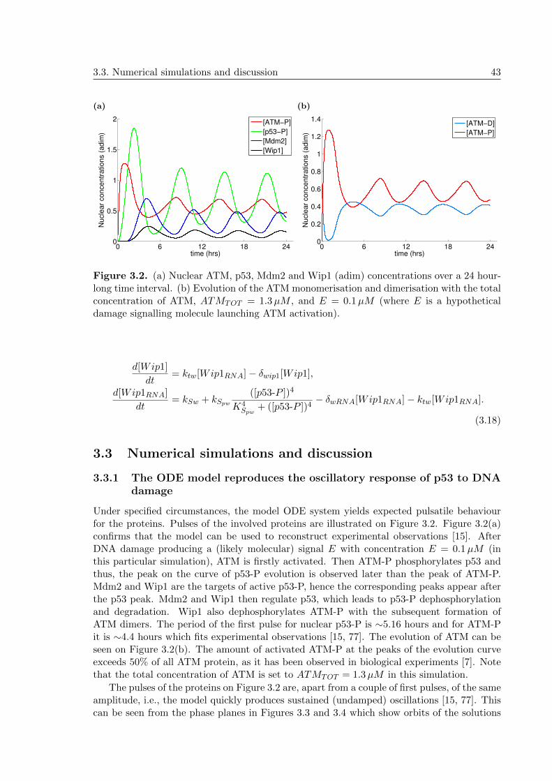
3.3. Numerical simulations and discussion 43
(a)
0 6 12 18 240
0.5
1
1.5
2
time (hrs)
Nucle
ar
concentr
ations (
adim
)
[ATM−P]
[p53−P]
[Mdm2]
[Wip1]
(b)
0 6 12 18 240
0.2
0.4
0.6
0.8
1
1.2
1.4
time (hrs)
Nucle
ar
concentr
ations (
adim
)
[ATM−D]
[ATM−P]
Figure 3.2. (a) Nuclear ATM, p53, Mdm2 and Wip1 (adim) concentrations over a 24 hour-long time interval. (b) Evolution of the ATM monomerisation and dimerisation with the totalconcentration of ATM, ATMTOT = 1.3µM , and E = 0.1µM (where E is a hypotheticaldamage signalling molecule launching ATM activation).
d[Wip1]
dt= ktw[Wip1RNA]− δwip1[Wip1],
d[Wip1RNA]
dt= kSw + kSpw
([p53-P ])4
K4Spw
+ ([p53-P ])4− δwRNA[Wip1RNA]− ktw[Wip1RNA].
(3.18)
3.3 Numerical simulations and discussion
3.3.1 The ODE model reproduces the oscillatory response of p53 to DNAdamage
Under specified circumstances, the model ODE system yields expected pulsatile behaviourfor the proteins. Pulses of the involved proteins are illustrated on Figure 3.2. Figure 3.2(a)confirms that the model can be used to reconstruct experimental observations [15]. AfterDNA damage producing a (likely molecular) signal E with concentration E = 0.1µM (inthis particular simulation), ATM is firstly activated. Then ATM-P phosphorylates p53 andthus, the peak on the curve of p53-P evolution is observed later than the peak of ATM-P.Mdm2 and Wip1 are the targets of active p53-P, hence the corresponding peaks appear afterthe p53 peak. Mdm2 and Wip1 then regulate p53, which leads to p53-P dephosphorylationand degradation. Wip1 also dephosphorylates ATM-P with the subsequent formation ofATM dimers. The period of the first pulse for nuclear p53-P is ∼5.16 hours and for ATM-Pit is ∼4.4 hours which fits experimental observations [15, 77]. The evolution of ATM can beseen on Figure 3.2(b). The amount of activated ATM-P at the peaks of the evolution curveexceeds 50% of all ATM protein, as it has been observed in biological experiments [7]. Notethat the total concentration of ATM is set to ATMTOT = 1.3µM in this simulation.
The pulses of the proteins on Figure 3.2 are, apart from a couple of first pulses, of the sameamplitude, i.e., the model quickly produces sustained (undamped) oscillations [15, 77]. Thiscan be seen from the phase planes in Figures 3.3 and 3.4 which show orbits of the solutions
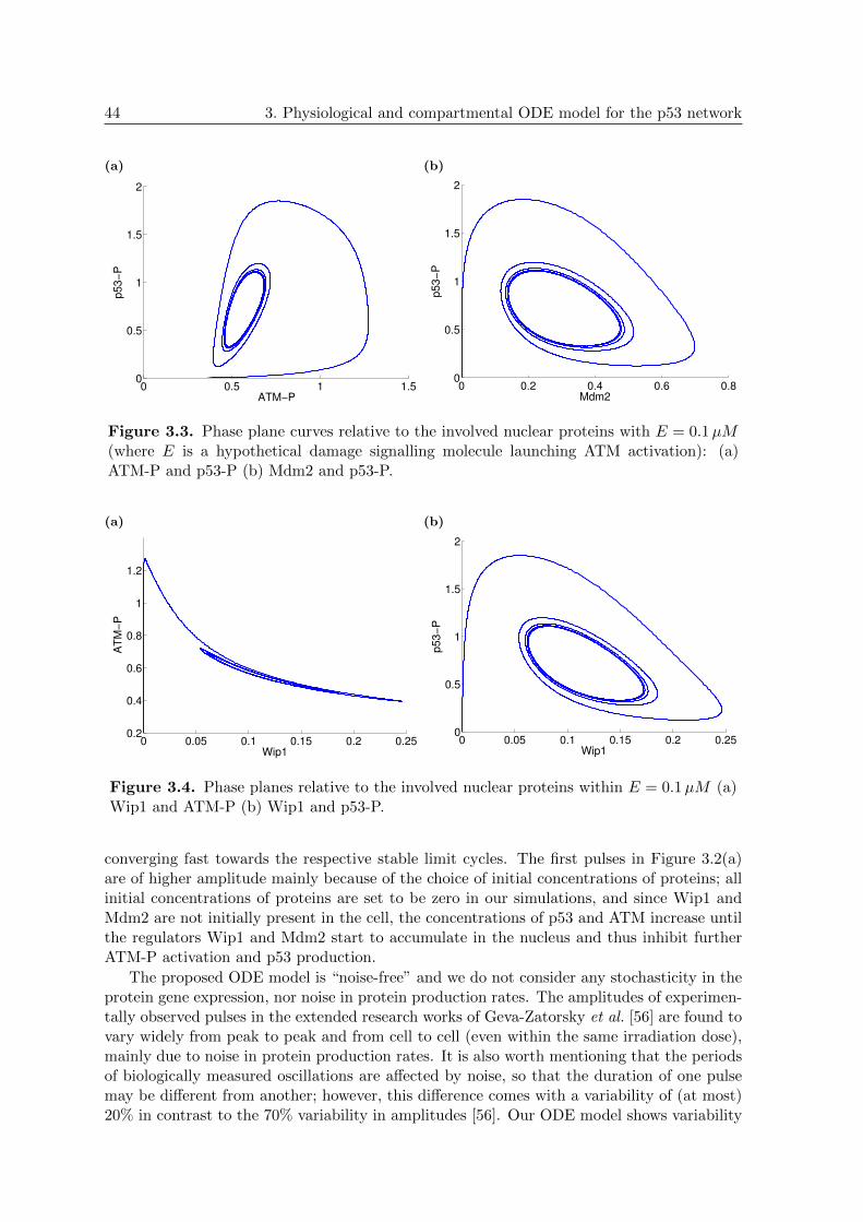
44 3. Physiological and compartmental ODE model for the p53 network
(a)
0 0.5 1 1.50
0.5
1
1.5
2
ATM−P
p53−
P
(b)
0 0.2 0.4 0.6 0.80
0.5
1
1.5
2
Mdm2
p53−
PFigure 3.3. Phase plane curves relative to the involved nuclear proteins with E = 0.1µM(where E is a hypothetical damage signalling molecule launching ATM activation): (a)ATM-P and p53-P (b) Mdm2 and p53-P.
(a)
0 0.05 0.1 0.15 0.2 0.250.2
0.4
0.6
0.8
1
1.2
Wip1
AT
M−
P
(b)
0 0.05 0.1 0.15 0.2 0.250
0.5
1
1.5
2
Wip1
p53−
P
Figure 3.4. Phase planes relative to the involved nuclear proteins within E = 0.1µM (a)Wip1 and ATM-P (b) Wip1 and p53-P.
converging fast towards the respective stable limit cycles. The first pulses in Figure 3.2(a)are of higher amplitude mainly because of the choice of initial concentrations of proteins; allinitial concentrations of proteins are set to be zero in our simulations, and since Wip1 andMdm2 are not initially present in the cell, the concentrations of p53 and ATM increase untilthe regulators Wip1 and Mdm2 start to accumulate in the nucleus and thus inhibit furtherATM-P activation and p53 production.
The proposed ODE model is “noise-free” and we do not consider any stochasticity in theprotein gene expression, nor noise in protein production rates. The amplitudes of experimen-tally observed pulses in the extended research works of Geva-Zatorsky et al. [56] are found tovary widely from peak to peak and from cell to cell (even within the same irradiation dose),mainly due to noise in protein production rates. It is also worth mentioning that the periodsof biologically measured oscillations are affected by noise, so that the duration of one pulsemay be different from another; however, this difference comes with a variability of (at most)20% in contrast to the 70% variability in amplitudes [56]. Our ODE model shows variability
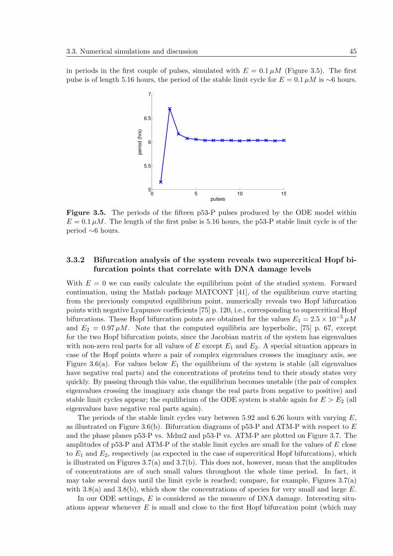
3.3. Numerical simulations and discussion 45
in periods in the first couple of pulses, simulated with E = 0.1µM (Figure 3.5). The firstpulse is of length 5.16 hours, the period of the stable limit cycle for E = 0.1µM is ∼6 hours.
0 5 10 155
5.5
6
6.5
7
pulses
period (
hrs
)
Figure 3.5. The periods of the fifteen p53-P pulses produced by the ODE model withinE = 0.1µM . The length of the first pulse is 5.16 hours, the p53-P stable limit cycle is of theperiod ∼6 hours.
3.3.2 Bifurcation analysis of the system reveals two supercritical Hopf bi-furcation points that correlate with DNA damage levels
With E = 0 we can easily calculate the equilibrium point of the studied system. Forwardcontinuation, using the Matlab package MATCONT [41], of the equilibrium curve startingfrom the previously computed equilibrium point, numerically reveals two Hopf bifurcationpoints with negative Lyapunov coefficients [75] p. 120, i.e., corresponding to supercritical Hopfbifurcations. These Hopf bifurcation points are obtained for the values E1 = 2.5× 10⁻⁵ µMand E2 = 0.97µM . Note that the computed equilibria are hyperbolic, [75] p. 67, exceptfor the two Hopf bifurcation points, since the Jacobian matrix of the system has eigenvalueswith non-zero real parts for all values of E except E1 and E2. A special situation appears incase of the Hopf points where a pair of complex eigenvalues crosses the imaginary axis, seeFigure 3.6(a). For values below E1 the equilibrium of the system is stable (all eigenvalueshave negative real parts) and the concentrations of proteins tend to their steady states veryquickly. By passing through this value, the equilibrium becomes unstable (the pair of complexeigenvalues crossing the imaginary axis change the real parts from negative to positive) andstable limit cycles appear; the equilibrium of the ODE system is stable again for E > E2 (alleigenvalues have negative real parts again).
The periods of the stable limit cycles vary between 5.92 and 6.26 hours with varying E,as illustrated on Figure 3.6(b). Bifurcation diagrams of p53-P and ATM-P with respect to Eand the phase planes p53-P vs. Mdm2 and p53-P vs. ATM-P are plotted on Figure 3.7. Theamplitudes of p53-P and ATM-P of the stable limit cycles are small for the values of E closeto E1 and E2, respectively (as expected in the case of supercritical Hopf bifurcations), whichis illustrated on Figures 3.7(a) and 3.7(b). This does not, however, mean that the amplitudesof concentrations are of such small values throughout the whole time period. In fact, itmay take several days until the limit cycle is reached; compare, for example, Figures 3.7(a)with 3.8(a) and 3.8(b), which show the concentrations of species for very small and large E.
In our ODE settings, E is considered as the measure of DNA damage. Interesting situ-ations appear whenever E is small and close to the first Hopf bifurcation point (which may

46 3. Physiological and compartmental ODE model for the p53 network
(a)
0.01
0.014
0.016
0.018
0.02
H
H
−2 −1 0 1 2 3
x 10 −3
−0.022
−0.02
−0.018
−0.016
−0.014
H
H
Re
Im
(b)
−5 −4 −3 −2 −1 05.9
5.95
6
6.05
6.1
6.15
6.2
6.25
6.3
6.35
log10
E
pe
rio
ds o
f sta
ble
lim
it c
ycle
s (
hrs
)
H
H
Figure 3.6. (a) A pair of eigenvalues crossing the imaginary axis for E = 2.5 × 10⁻⁵ andE = 0.97, revealing thus the existence of two Hopf bifurcation points. (b) Evolution of theperiod of stable limit cycles maintaining between the two Hopf bifurcation points; E is in thelogarithmic scale.
correspond to a few DSB only) and when E is very big (which may correspond to seriousDNA damage and many DSB). In the first case, the concentration of ATM-P does not evenoscillate for the values of E close to E1, see Figure 3.8(a). The ATM trajectory on Fig. 3.8(a)tends to a steady state of low level; however, this small concentration of ATM-P can still elicitp53-P pulses (rather moderate compared to Fig. 3.2(a)). This may contradict experimentalobservations that show oscillating ATM in the DDR [15]; note, however, that those experi-ments were performed with the exposure of cells to 10 Gy of γ-irradiation and not to dosescausing only a few DSB (which may correspond to E as small as E1). On the other hand,other works show evidence that only very small amounts of ATM (even not detectable) canstill elicit relevant p53 signalling [13, 159]. Indeed, DNA damage at E ≈ E1 may correspondto occasional DNA DSB which do not need ATM for DNA repair and only moderate ATMis produced which is still efficient in p53 activation.
ATM oscillations are damped and disappear for E greater than E2. Once the oscillationshave vanished, they do not appear again with further increasing values of E. Figure 3.8(b),for example, shows the protein dynamics for E = 10µM . In this case ATM is almost fullyactivated and only small deviations in ATM concentration can be seen. Hence, we canspeculate that if E is high and it is impossible to repair DNA DSB, then Wip1 phosphataseactivities towards ATM are inhibited, the active ATM achieves its maxima and apoptosisis initiated. However, the latter suggestion is not supported by experimental observations;in fact, there is no paper in the literature, to our best knowledge, clarifying ATM activityand location in single cells committing apoptosis. Thus, ATM may oscillate whenever it isnecessary for a proper cell response to DNA damage of an alive cell, and once E becomestoo high, oscillations disappear and the cell dies. Such interpretation, however, may requireE to be dependent not only on DNA damage levels but also on other factors amplifying theabundance of E, possibly with the contribution of proapoptotic proteins.
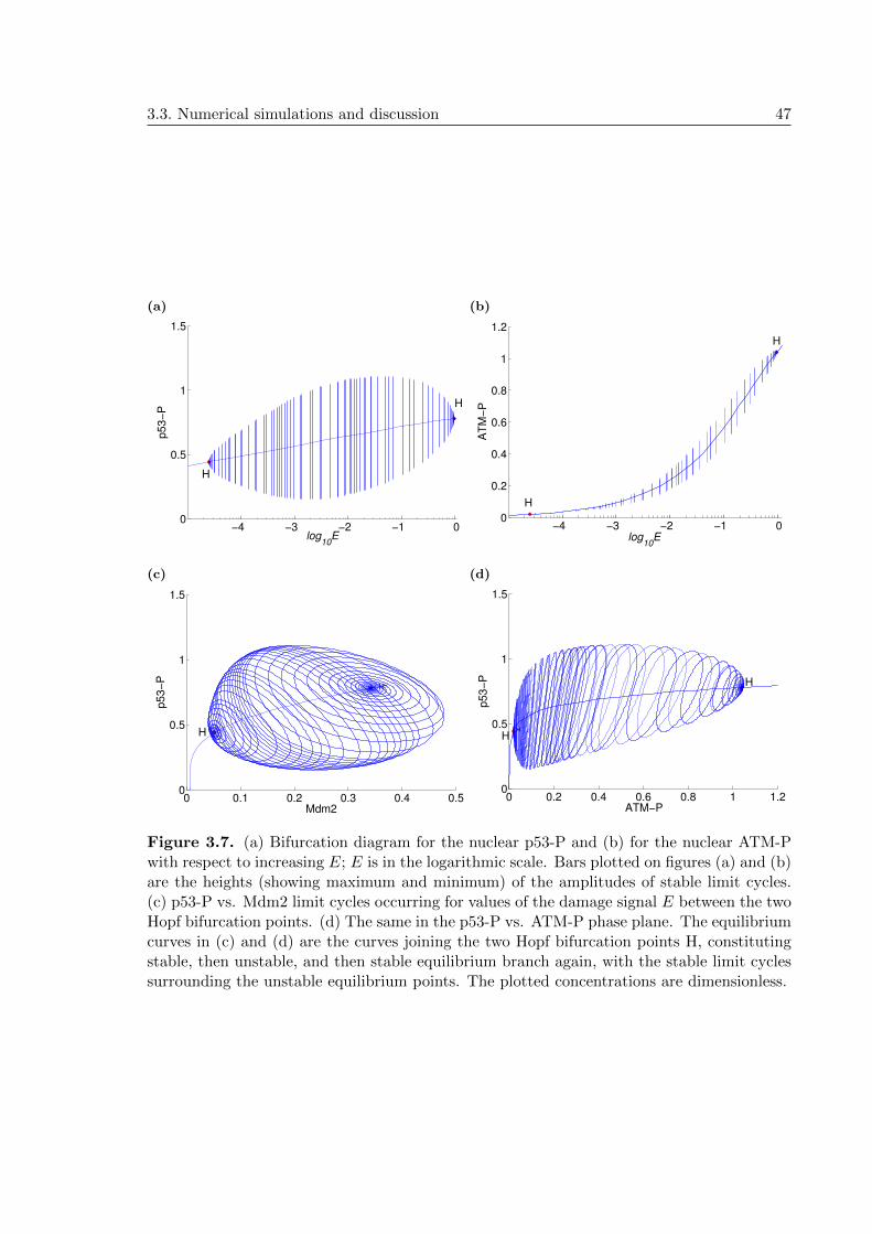
3.3. Numerical simulations and discussion 47
(a)
−4 −3 −2 −1 00
0.5
1
1.5
log10
E
p53−
P
H
H
(b)
−4 −3 −2 −1 00
0.2
0.4
0.6
0.8
1
1.2
log10
E
AT
M−
P
H
H
(c)
0 0.1 0.2 0.3 0.4 0.50
0.5
1
1.5
Mdm2
p53−
P
H
H
(d)
0 0.2 0.4 0.6 0.8 1 1.20
0.5
1
1.5
ATM−P
p53−
P
H
H H
H
Figure 3.7. (a) Bifurcation diagram for the nuclear p53-P and (b) for the nuclear ATM-Pwith respect to increasing E; E is in the logarithmic scale. Bars plotted on figures (a) and (b)are the heights (showing maximum and minimum) of the amplitudes of stable limit cycles.(c) p53-P vs. Mdm2 limit cycles occurring for values of the damage signal E between the twoHopf bifurcation points. (d) The same in the p53-P vs. ATM-P phase plane. The equilibriumcurves in (c) and (d) are the curves joining the two Hopf bifurcation points H, constitutingstable, then unstable, and then stable equilibrium branch again, with the stable limit cyclessurrounding the unstable equilibrium points. The plotted concentrations are dimensionless.

48 3. Physiological and compartmental ODE model for the p53 network
(a)
0 6 12 18 24 30 36 42 480
0.1
0.2
0.3
0.4
0.5
time (hrs)
Nu
cle
ar
co
nce
ntr
atio
ns (
ad
im)
[ATM−P]
[p53−P]
(b)
0 6 12 18 240
0.5
1
1.5
2
time (hrs)
Nucle
ar
concentr
ations (
adim
)
[ATM−P]
[p53−P]
[Mdm2]
[Wip1]
Figure 3.8. (a) Nuclear p53-P and ATM-P (adim) concentrations from the ODE systemfor E = E1 = 2.5 × 10⁻⁵ µM . The concentration of ATM-P converges to the equilibriumpoint ( which is equal to 0.02) and the concentration of p53-P tends to a stable limit cycle.(b) Nuclear ATM-P, p53-P, Mdm2 and Wip1 (adim) concentrations for E = 10µM . Theoscillations of ATM-P are of small amplitude, getting even smaller with further increasing E;ATMTOT = 1.3µM .
3.3.3 Two negative feedback loops and a compartmental distribution ofcellular processes produce sustained oscillations
In order to show that the oscillating ATM protein plays an active role in achieving p53 pulseswe made several simulations to test different possibilities and thus we explored the systemin more details. For example, the model can be used to mimic the observed inhibition ofp53 (an Mdm2) pulses following one full ATM pulse [15]; this is illustrated on Figures 3.9,where ATM is inhibited after one pulse. We can see one complete pulse of ATM followed bythe pulses in p53, Mdm2 and Wip1 concentration. Wip1 then blocks further ATM activation(in the corresponding equation (3.4) of ATM dephosphorylation by Wip1, the Michaelis rateKdph2 is set to be very small, Kdph2 = 0.0001). Although the first pulses of the p53 and Mdm2proteins are induced they are not sufficient to produce subsequent pulses if ATM signallingis impeded.
Other tests when we inhibit, respectively,
• the negative feedback Wip1 a ATM (kdph2 = 0 in (3.4), Figure 3.12(a)),
• the positive feedback ATM → p53 (kph1 = 0 in (3.14), Figure 3.12(b)),
• the negative feedback Wip1 a p53-P (kdph1 = 0 in (3.14), Figure 3.12(c)),
• the positive feedback p53-P →Wip1 (kSpw = 0, Figures 3.12(d) and (e)),
produce either damped oscillations or do not produce oscillations at all. The ATM and Wip1proteins must thus be involved in the p53-Mdm2 dynamics in order to produce sustained p53oscillations.
The p53-Mdm2 negative feedback cannot be omitted either, since the inhibition of Mdm2activity on p53 (kub = 0 in (3.14), see Figure 3.10(a)) or the inhibition of the transcriptionalactivity of p53-P on Mdm2 (kSpm = 0 in (3.15), Figures 3.12(f)) does not produce oscillations.

3.3. Numerical simulations and discussion 49
(a)
0 6 12 18 240
0.2
0.4
0.6
0.8
1
1.2
1.4
time (hrs)
Nucle
ar
concentr
ations (
adim
)
[ATM−P]
[p53−P]
[Mdm2]
[Wip1]
(b)
0 6 12 18 240
0.2
0.4
0.6
0.8
1
1.2
1.4
time (hrs)
Nucle
ar
concentr
ations (
adim
)
[ATM−D]
[ATM−P]
Figure 3.9. (a) Nuclear ATM, p53, Mdm2 and Wip1 (adim) concentrations over a 24 hour-long time interval following ATM inhibition after one full pulse. (b) Evolution of the ATMmonomerisation and dimerisation with the total concentration of ATM, ATMTOT = 1.3µM ,and E = 0.1µM , following ATM inhibition after one full pulse.
We can further ask whether the two feedback loops without strict location of proteinsin the compartments can lead to p53 oscillations. Merging protein dynamics into one com-partment (the whole cell), i.e. omitting exchange of the species between the nucleus and thecytoplasm but rather considering both compartments as the one where proteins and theirmRNA can freely migrate, is not, however, sufficient in producing sustained oscillations. Fig-ure 3.10(b) shows the concentrations of proteins in the case of E = 0.1µM . Similarly, otherchoices of E exhibit concentrations of proteins converging to their steady states (bifurcationanalysis does not reveal any significant point).
Hence, the feedbacks p53 → Mdm2 a p53 and ATM → p53 → Wip1 a ATM togetherwith compartmental distribution of proteins result in sustained oscillations, and neglectingany part of these three components fails to produce sustained oscillations.
3.3.4 ATM threshold required for initiation of p53 pulses
Note again that there are two significant points in the range of the signal E. In particular,these are the two Hopf bifurcation points, E1 = 2.5× 10⁻⁵ µM and E2 = 0.97µM : values ofE starting from E1 are sufficient to elicit sustained oscillations in the concentration of p53,and the second Hopf bifurcation point E2 is the critical point at which stable limit cycles(otherwise said, sustained oscillations of the proteins) disappear. This point thus may marka decision for the cell not to go on in DNA DSB repairing processes, and rather to startapoptosis. A relation to a supposed apoptotic threshold which is proposed in [73] remains tobe further established.
The hypothetical substrate E is supposed to be produced by DNA DSB sensors (e.g.,the MRN complex bound to the DNA break sites) and/or by some changes in the chromatinstructure; E may be also affected by other prosurvival and proapoptotic factors. Then E isdelivered to the ATM dimers and promotes ATM activation. Interestingly, an amount of Eas small as E1 can (for the value of total ATM protein ATMTOT = 1.3µM) activate ATM atthe concentration ∼0.02 µM , Figure 3.8(b), that is sufficient to produce oscillations in p53.
Note, however, that the Hopf bifurcation points are dependent on the total nuclear con-

50 3. Physiological and compartmental ODE model for the p53 network
(a)
0 6 12 18 240
0.5
1
1.5
2
2.5
3
time (hrs)
Nucle
ar
concentr
ations (
adim
)
[ATM−P]
[p53−P]
[Mdm2]
[Wip1]
(b)
0 6 12 18 240
0.5
1
1.5
2
time (hrs)
Nucle
ar
concentr
ations (
adim
)
[ATM−P]
[p53−P]
[Mdm2]
[Wip1]
Figure 3.10. (a) Nuclear ATM, p53, Mdm2 and Wip1 (adim) concentrations over a 24hour-long time interval, E = 0.1µM , in the case when Mdm2-mediated ubiquitination ofp53 is inhibited, kub = 0. (b) Nuclear ATM, p53, Mdm2 and Wip1 (adim) concentrationsover a 24 hour-long time interval and E = 0.1µM in the case when only one compartmentis considered.
centration of ATM, which is denoted by ATMTOT . Indeed, Figure 3.11(a) shows the evolutionof the Hopf bifurcation points with respect to ATMTOT (on the y-axis). We can see thatthe values of the first Hopf point E1 do not change dramatically and they range between1, 17 × 10−5 (which corresponds to ATMTOT = 10µM) and 3.5 × 10⁻⁵ (which correspondsto ATMTOT = 0.78µM). The dependence of E2 on ATMTOT seems to be more intrigu-ing. Similarly to E1, the Hopf bifurcation point E2 increases with decreasing ATMTOT ,and asymptotically reaches values corresponding to ATMTOT ≈ 0.77µM , Figure 3.11(a).In other words, the system has two Hopf bifurcation points for ATMTOT > 0.77µM (withsimilar bifurcation diagrams between these points Figure 3.11(b)). The system possessesonly one Hopf bifurcation point between ATMTOT = 0.082 and 0.77µM which determinesstable solution and unstable solution (stable limit cycle). The system does not have any Hopfbifurcation point for ATMTOT < 0.082µM .
This suggests that there is a threshold in the concentration of ATM that is necessary forthe proper oscillatory response of p53. Indeed, p53 can exhibit oscillations in the cells withthe total amount of ATM exceeding 0.082µM (in our modelling setting). Notably, whenthese cell are exposed to agents causing DNA damage which corresponds to E = E1, that isthe smallest value of E for which p53 shows oscillations, the activated ATM-P converges to asteady state which is independent of the total ATM molecules in the system. This equilibriumvalue of ATM-P is ∼0.02 µM . See, for example, Figure 3.8(a) where the dynamics of p53 isshown for E = E1 = 2.5×10⁻⁵ µM and ATMTOT = 1.3µM . Note that it has been observedthat only a fraction of ATM molecules can be sufficient to activate p53 and thus to initiateDDR [159]. However, a certain threshold for initial ATM concentration is supposed to existto initiate the ATM signalling pathway [15]. Our model confirms this hypothesis and, inaddition, we propose that the value of activated ATM-P is independent of the total ATMmolecules in the cell.

3.4. Conclusion from the ODE modelling 51
(a)
−6 −4 −2 00
2
4
6
8
10
log10
E
AT
M T
OT
E2
E1 E2
E1
(b)
−5
0
0
5
100
0.5
1
1.5
2
H
log10
E
H
H
H
ATM TOT
p53−
P
Figure 3.11. (a) The evolution curves of both Hopf bifurcation points (curves in brown andblack colours). The plotted Hopf points E1 and E2 are computed for ATMTOT = 10µM ,the Hopf points E1 and E2 are computed for ATMTOT = 0.78µM . E is in the logarithmicscale. (b) Bifurcation diagram of p53-P with respect to changing ATMTOT and E.
3.4 Conclusion from the ODE modelling
Explaining experimentally observed p53 oscillations in human cancer cells after exposure ofthe cells to γ-irradiation [15, 77, 56] is a mathematical modelling challenge, especially in theperspective of proposing p53-mediated anticancer drug-induced cell cycle arrest/apoptoticpredictions. The ODE model presented here is the extension of a previous work by Dimitrioet al. [42, 43]. It presents the dynamics of the “guardian of the genome” p53, that plays es-sential parts in cell responses to DNA damage and checkpoint signalling. The compartmentaldistribution of proteins in a cell is taken into account and it is shown that such compart-mental recognition of cellular events allows to reconstruct the pulsatile behaviour of proteinswithout the need to introduce any time delay in their dynamics.
The oscillatory dynamics of the involved proteins can be speculatively explained as peri-odical testing of the presence of DNA damage: if unrepaired DNA DSB still exist, additionalpulses of both phosphorylated ATM and p53 are triggered. More precisely, the level of phos-phorylated ATM-P increases in response to DSB and ATM-dependent phosphorylation ofp53 leads to its nuclear stabilisation and activation. p53 acts as a transcription factor of abench of proteins employed in the cell cycle arrest and DNA damage repair, but also proteinsinitiating an irreversible decision (such as senescence or apoptosis) and prosurvival proteinswhich are trying to terminate the DDR and release the cell from the cell cycle arrest. Wip1and Mdm2 proteins are such homeostatic agents since they act, respectively, through dephos-phorylation and ubiquitination of ATM and p53, thus rendering them inactive. When p53levels are reduced, ATM is released to re-examine the DNA. If the number of DSB remainsabove a certain threshold, the pathway becomes reactivated, leading to a second pulse ofATM and p53, and this continues until the DNA is repaired or until the cell decides to startapoptosis [15].
The original models of Dimitrio et al. [42, 43] involve ATM as a direct measure of DNAdamage, in the form of a parameter that remains constant in the studied time interval.It has been experimentally shown, however, that a pulsatile behaviour of p53 cannot bereached without the active and oscillating ATM [15]. In addition, there exist biological

52 3. Physiological and compartmental ODE model for the p53 network
studies that confirm a role of ATM in cancer cell apoptosis induced, for example, by ionisingradiations [83]. Hence, in this extended modelling work we consider ATM as an essentialpart of the DNA damage signalling pathway, varying with the time, that after ATM dimerdissociation and activation phosphorylates p53 and thus initiates p53 transcriptional activitytowards proarrest and proapoptotic genes (for example, p21 and 14-3-3σ on the proarrest side,and Pig3, Apaf1 and PUMA on the proapoptotic side). It was shown here that a certainthreshold of ATM-P is required for the p53 oscillations (as proposed by experimentalists) andthat this threshold does not depend on the total abundance of ATM in the cell.
The p53 protein responds to a variety of cellular stresses (such as those causing DNAstrand breaks, e.g., cytotoxic drug insults) through the transcription mode of protein pro-duction. Despite the complexity of all signalling pathways occurring in the stressed cells andthe production of proteins involved therein, we can conclude that the pathway including p53activation can be successfully reconstructed by our compartmental model that, in particu-lar, takes into account the ATM-p53-Mdm2-Wip1 dynamics as it has been observed in thescientific literature on the subject [15, 136, 7, 13], and as it is summarised in details in thebiological background.
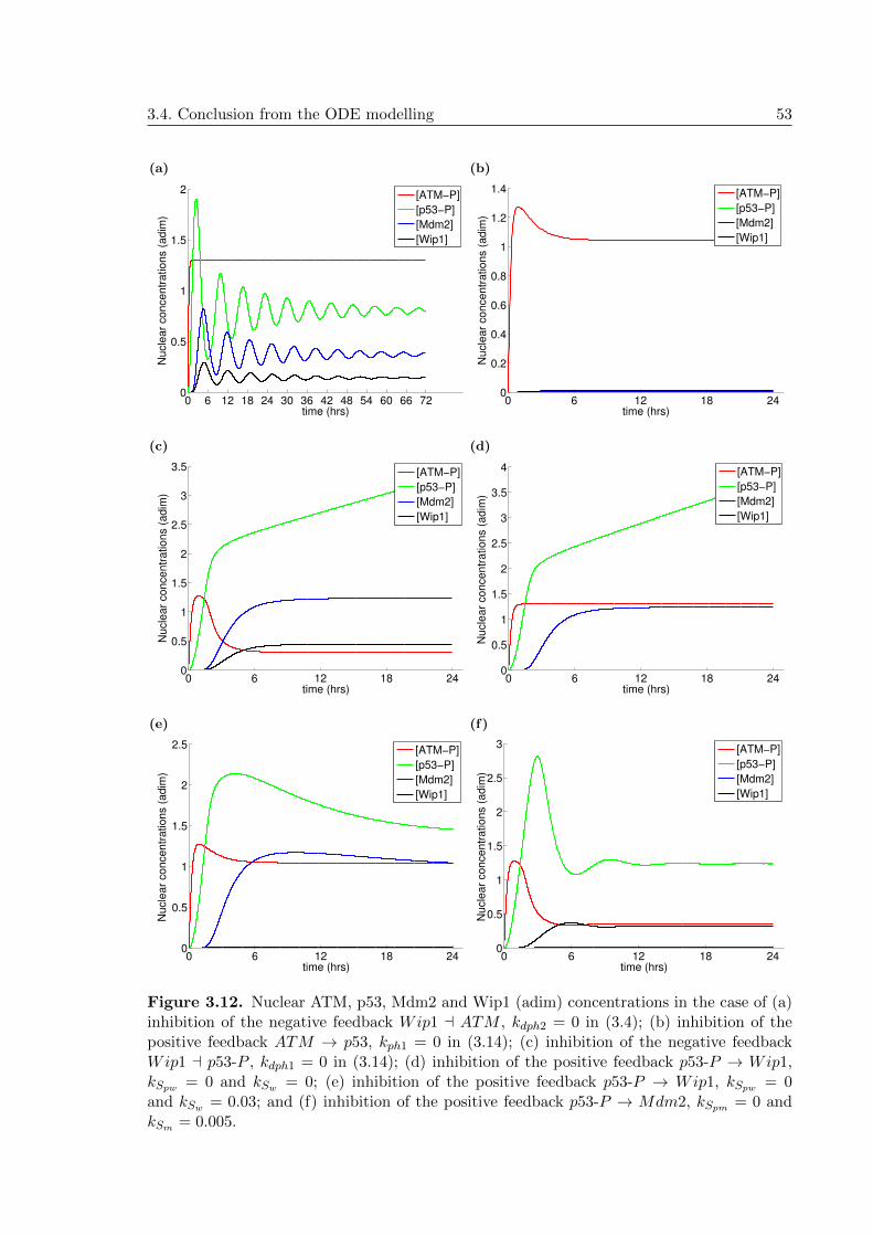
3.4. Conclusion from the ODE modelling 53
(a)
0 6 12 18 24 30 36 42 48 54 60 66 720
0.5
1
1.5
2
time (hrs)
Nu
cle
ar
co
nce
ntr
atio
ns (
ad
im)
[ATM−P]
[p53−P]
[Mdm2]
[Wip1]
(b)
0 6 12 18 240
0.2
0.4
0.6
0.8
1
1.2
1.4
time (hrs)
Nu
cle
ar
co
nce
ntr
atio
ns (
ad
im)
[ATM−P]
[p53−P]
[Mdm2]
[Wip1]
(c)
0 6 12 18 240
0.5
1
1.5
2
2.5
3
3.5
time (hrs)
Nu
cle
ar
co
nce
ntr
atio
ns (
ad
im)
[ATM−P]
[p53−P]
[Mdm2]
[Wip1]
(d)
0 6 12 18 240
0.5
1
1.5
2
2.5
3
3.5
4
time (hrs)
Nu
cle
ar
co
nce
ntr
atio
ns (
ad
im)
[ATM−P]
[p53−P]
[Mdm2]
[Wip1]
(e)
0 6 12 18 240
0.5
1
1.5
2
2.5
time (hrs)
Nu
cle
ar
co
nce
ntr
atio
ns (
ad
im)
[ATM−P]
[p53−P]
[Mdm2]
[Wip1]
(f)
0 6 12 18 240
0.5
1
1.5
2
2.5
3
time (hrs)
Nu
cle
ar
co
nce
ntr
atio
ns (
ad
im)
[ATM−P]
[p53−P]
[Mdm2]
[Wip1]
Figure 3.12. Nuclear ATM, p53, Mdm2 and Wip1 (adim) concentrations in the case of (a)inhibition of the negative feedback Wip1 a ATM , kdph2 = 0 in (3.4); (b) inhibition of thepositive feedback ATM → p53, kph1 = 0 in (3.14); (c) inhibition of the negative feedbackWip1 a p53-P , kdph1 = 0 in (3.14); (d) inhibition of the positive feedback p53-P → Wip1,kSpw = 0 and kSw = 0; (e) inhibition of the positive feedback p53-P → Wip1, kSpw = 0and kSw = 0.03; and (f) inhibition of the positive feedback p53-P → Mdm2, kSpm = 0 andkSm = 0.005.

54 3. Physiological and compartmental ODE model for the p53 network
Parameter Value Units Description
kph1 3 min−1 velocity of ATM-P-dep. ph. of p53
Kph1 0.1 µM Michaelis rate of ATM-P-dep. ph. of p53
kdph1 78 min−1 velocity of Wip1-dep. deph. of p53-P
Kdph1 25 µM Michaelis rate of Wip1-dep. deph. of p53-P
kub 10 min−1 velocity of Mdm2-dep. ubiq. of p53
Kub 1.01 µM Michaelis rate of Mdm2-dep. ubiq. of p53
kS 0.015 µM/min basal synthesis rate of p53
kSm 0.005 µM/min basal synthesis rate of Mdm2 mRNA
kSpm 1 µM/min velocity of Mdm2 mRNA transcription
KSpm 0.1 µM Michaelis rate of Mdm2 mRNA transcription
ktm 1 min−1 translation rate for Mdm2
kSw 0.03 µM/min basal synthesis rate of Wip1 mRNA
kSpw 1 µM/min velocity of Wip1 mRNA transcription
KSpw 0.1 µM Michaelis rate of Wip1 mRNA transcription
ktw 1 min−1 translation rate for Wip1
kph2 15 min−1 velocity of ATM activation by E
Kph2 1 µM Michaelis rate of ATM activation by E.
kdph2 96 min−1 velocity of Wip1-dep. deph. of ATM-P
Kdph2 26 µM Michaelis rate of Wip1-dep. deph. of ATM-P
δp53 0.2 min−1 p53 degradation rate
δmdm2 0.16 min−1 Mdm2 degradation rate
δmRNA 0.0001 min−1 Mdm2 mRNA degradation rate
δwip1 0.2 min−1 Wip1 degradation rate
δwRNA 0.001 min−1 Wip1 mRNA degradation rate
Vr 10 adim nucleus:cytoplasm volume ratio
pp53 0.083 min−1 permeability rate for p53
pmdm2 0.04 min−1 permeability rate for Mdm2
pmRNA 0.083 min−1 permeability rate for Mdm2 mRNA
pwip1 0.083 min−1 permeability rate for Wip1
pwRNA 0.083 min−1 permeability rate for Wip1 mRNA
E 0.1 µM concentration of “the damage signal”
ATMTOT 1.3 µM total ATM concentration
Table 3.1. Set of parameter values for the compartmental ODE model (3.16) and (3.17)published in [47]. Most of the parameters for the ODE model are taken from [42, 43], someother are taken from [136, 137]. In the table, “dep.” stands for dependent, “ubiq.” forubiquitination, “ph.” for phosphorylation and “deph.” for dephosphorylation.

4
Reaction-diffusion systems forprotein networks
Spatio-temporal dynamics of a variety of proteins is, among other things, regulatedby post-translational modifications of these proteins. Such modifications can thusinfluence stability and biochemical activities of the proteins, activity and stability oftheir upstream targets within specific signalling pathways. Commonly used mathe-matical tools for such protein-protein (and/or protein-mRNA) interactions in singlecells such as Michaelis-Menten and Hill kinetics, yielding a system of ordinary dif-ferential equations (as we have seen in the previous chapter), can be extended intopartial differential equations by taking into account a more realistic spatial repre-sentation of the environment where these reactions occur. This chapter aims toconnect physiological ODE models with their PDE counterparts in the simplest pos-sible case—by involving a space variable and allowing species to diffuse across adomain under consideration.
Organisation of the chapter is as follows: The first of two sections in this chapter,Section 4.2, gives a rather general introduction to reaction-diffusion equations fora protein pathway occurring in a cell composed of two compartments: nucleus andcytoplasm. Section 4.3 presents the Leloup–Goldbeter model for the FRQ protein.Reaction-diffusion models for the p53 protein are left to other chapters. Note that toour best knowledge, the reaction-diffusion Leloup–Goldbeter model is newly presentedhere.
Partial results presented in this chapter were published in [45],
[45] J. Elias and J. Clairambault. Reaction-diffusion systems for spatio-temporalintracellular protein networks: A beginners guide with two examples. Computa-tional and Structural Biotechnology Journal, 10(16):12–22, 2014.
4.1 Introduction to spatio-temporal modelling
In the modelling framework under consideration, all interactions occur in a cell divided intotwo compartments, the nucleus and the cytoplasm, connected by the semipermeable nuclearmembrane and bounded by the impermeable cell membrane, Figure 4.1. Passive transportmechanism discussed in Section 2.4 is modelled by the Kedem–Katchalsky boundary condi-
55

56 4. Reaction-diffusion systems for protein networks
tions (which can be derived from the Fick’s first law). Thus, in addition to the diffusion ofspecies across a compartment, species can migrate from one compartment to another throughthe nuclear membrane. As an example, the circadian rhythm for concentration of the FRQprotein in Neurospora crassa is presented.
One of the simplest ‘protein-mRNA’ models is a nonlinear biochemical oscillator proposedby Goodwin in 1965 [57] that simulates expression of a single gene controlled by its proteinproduct P , thus, closing the negative feedback loop. In particular, the equations appearingin the original Goodwin model are, respectively,
d[mRNA]
dt=
a1
A1 + k1[P ]− δ1,
d[P ]
dt= a2[mRNA]− δ2,
reporting here only production (transcription in the first equation and translation in thesecond) and degradation terms (δ1 and δ2).
Based on this model, a compartmental ODE model for the circadian clock rhythm ofthe FRQ protein expressed during a day in Neurospora crassa was proposed by Leloup andGoldbeter [85]. The model includes expression of the frq gene in the nucleus, a process thatis influenced by available light, and translation of FRQ mRNA into FRQ in the cytoplasmthat, afterwards, enters the nucleus and negatively regulates the transcription of its gene, asit is observed in vivo in [4].
The spatial organisation of the cell, however, suggests to consider migration of the in-volved species in the cytosol and between the compartments, and thus to model a proteinsignalling more realistically by including diffusivities of the species and by setting particulartranslocation conditions to model exchanges of the species between the compartments. Thus,one has to deal with coupled systems of nonlinear evolution partial differential equations(PDEs) for the concentrations of the species in the nucleus and in the cytoplasm with trans-mission boundary conditions (BC) imposed on the inner nuclear envelope and on the outercellular membrane (Robin-like and zero-flux BC in our modelling setting).
The aim of this chapter is to attract attention to reaction-diffusion equations for proteinspatio-temporal signalling rising from protein-protein (and/or protein-mRNA) interactionsin the two compartments of a cell, nucleus and cytoplasm, and from migration of the speciesin and between these compartments. Since it is impossible in general to derive analyticalsolutions for such coupled systems, numerically, passing to a weaker notion of solution, itcan be proved to exist (e.g., in Lipschitz domains as the cellular domains are assumed to bein our approach), for instance by the Rothe method. This method is applied to a reversibleenzyme reaction in Appendix B and can be easily adapted to more sophisticated problems,as the Leloup–Goldbeter FRQ model in this chapter and ATM-p53-Wip1-Mdm2 models inthe chapters that follow.
4.2 Reaction-diffusion models for protein intracellular net-works
Having in mind to represent the signalling of any protein in individual cells whose activity isdetermined by its post-translational modifications, one can write as many reactions as neces-sary to sufficiently describe a desired protein dynamics. The Law of Mass Action, Michaelis-Menten and Hill kinetics turn protein-protein interactions and transcription of genes intoproteins into a system of ODEs. Since the spatial representation of signalling pathways canreveal diffusion patterns that are hidden in ODEs, one might consider a system of PDEs

4.2. Reaction-diffusion models for protein intracellular networks 57
Ω2Ω1
Γ2
Γ1
n1
n2
Figure 4.1. Cell scheme: the nucleus Ω1, the cytoplasm Ω2, the nuclear membrane Γ1 andthe cell membrane Γ2; n1 and n2 are the unit normal vectors oriented outward from Ω1 andΩ2, respectively.
instead of ODEs. In PDEs, the protein dynamics in cells is particularly endowed with diffu-sivity rates and with some transmission conditions on the nuclear and cell (possibly other)membranes to represent, respectively, migration of species in and their exchange betweenthe cellular compartments and between cells themselves. In the sections that follow we showtwo examples of oscillators given by reaction-diffusion PDEs [22, 110]. The first one is basedon the commonly known and used Leloup–Goldbeter ODE model for circadian rhythms ofthe protein FRQ in Neurospora [85] (Section 4.3)1. The second one is a PDE model for thep53 intracellular dynamics following DNA damage in mammalian cells (Chapters 5 and 6).Another example of a signal transduction modelled by reaction-diffusion equations, moreprecisely, a model of Ran-driven transport process was studied in [134].
In cellular settings, a general coupled reaction diffusion system can be written as follows,
du
dt− div(D∇u) = f(u) in [0, T ]× Ω1,
dv
dt− div(D∇v) = g(v) in [0, T ]× Ω2,
+ boundary conditions on Γ1 and Γ2
(4.1)
where u = (u1, . . . , uN )T , ui = ui(t, x) : [0, T ]×Ω1 → R and v = (v1, . . . , vN )T , vi = vi(t, x) :[0, T ] × Ω2 → R for i = 0, 1, . . . , N − 1 are the nuclear and cytoplasmic concentrationsof N chemicals, N > 0, T > 0, f : RN → RN and g : RN → RN collect reaction andproduction/degradation terms for all N species (some of them can be equal to zero); avoidingany cross-diffusion, D is a diagonal N -by-N matrix with the diffusivities on the diagonal,and div is the divergence operator. The domains Ω1 and Ω2 represent the nucleus and thecytoplasm, respectively, assumed to be Lipschitz domains [130], Γ1 is the nuclear membraneand Γ2 is the cell membrane. The geometry of a cell under consideration is sketched inFigure 4.1, that in our very simplified framework represents a cell as big as 10−100µm or so,which is able to proliferate and which can have heterogeneous shape. However, we excludecells of complicated structures and morphologies such as neurons or muscle cells.
As previously outlined, we will consider zero-flux boundary conditions on the outer cell
membrane Γ2, i.e.∂vi∂n2
= 0 for i = 0, 1 . . . , N − 1 where n2 is the unit normal vector oriented
outward from the cell, Figure 4.1. Although species with molecular weight over 40kDa usuallyuse active transport mechanisms to be translocated from one compartment to another, for thesake of simplicity, only passive transport process driven by the difference in concentrations
1The Leloup–Goldbeter model for FRQ in Neurospora has been later slightly modified by the authors,adding two phosphorylation equations, to represent circadian rhythms of the protein PER in Drosophila[84, 31].

58 4. Reaction-diffusion systems for protein networks
at both sides of the nuclear membrane, modelled by the Kedem–Katchalsky BC, is used here[23, 43, 46, 112], for additional details see Section 2.4. In particular, export/import of thenuclear species is modelled by
−Di∂ui∂n1
= −pi(vi − ui) (4.2)
and export/import of the cytoplasmic species by
Di∂vi∂n1
= −pi(ui − vi), (4.3)
where n1 is the unit normal vector oriented outward from the nucleus (therefore, the BCin (4.3) come with a different sign), and pi are the permeabilities of the membrane for eachspecies i = 0, 1, . . . , N − 1. Recall that if a chemical is assumed to migrate between thecompartments in one direction only, e.g. mRNA is supposed to move from the transcriptionsites in the nucleus to the cytoplasm and not the other way round, then this can easily bemodelled by omitting either vi or ui in (4.2) and (4.3), cf. (4.6)-(4.8) below.
In addition to the boundary conditions, we will assume initial conditions for each speciesi = 0, 1, . . . , N − 1 to be non-negative functions ui(t = 0, x) = u0
i (x) ≥ 0 and vi(t = 0, x) =v0i (x) ≥ 0 belonging to L2(Ω1) and L2(Ω2), respectively.
4.3 The Leloup–Goldbeter model for the Neurospora crassacircadian clock
4.3.1 The frequency protein and circadian clock
Circadian clock in Neurospora controls the pattern of asexual development [44] and a centralcomponent of sustained rhythms is the FRQ protein (a long form of 989 amino acids and ashort form of 890 amino acids) encoded by the frq clock gene [4]. The oscillator consists ofa self-control of frq transcription, i.e. a negative feedback loop in which frq is synthesisedinto the FRQ protein (both short and long forms are required for robust rhythmic responses)which, in turn, acts to reduce intensity of frq transcription into mRNA [44].
Making the Neurospora clock start at midnight when FRQ mRNA and the FRQ proteinattain low levels in concentration, we see that transcription of the gene increases and mRNAreaches its peak in the midmorning about 4 hours before the peak of the total FRQ. FRQenters the nucleus where it contributes to inhibit gene transcription through the interactionwith other factors (WC-1 and WC-2) required in the frq gene transcription [55, 44]. Partialphosphorylation of FRQ leads to its initial degradation as soon as it enters the nucleus.Degradation then increases with more extensive FRQ phosphorylation through the earlynight [157, 44].
4.3.2 Spatio-temporal Leloup–Goldbeter PDE model for FRQ
Circadian clock represented by sustainedly oscillating concentration of the FRQ protein ismodelled by Leloup and Goldbeter [85] via the following ODE equations,
d[FRQmRNA]
dt= Vs
Kr
Kr + ([FRQ](n))r− Vm
[FRQmRNA]
Km + [FRQmRNA],
d[FRQ](c)
dt= ks[FRQmRNA]− Vd
[FRQ](c)
Kd + [FRQ](c)− k1[FRQ](c) + k2[FRQ](n),
d[FRQ](n)
dt= k1[FRQ](c) − k2[FRQ](n).
(4.4)
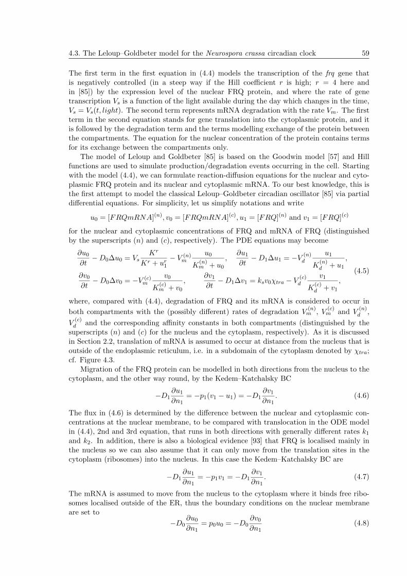
4.3. The Leloup–Goldbeter model for the Neurospora crassa circadian clock 59
The first term in the first equation in (4.4) models the transcription of the frq gene thatis negatively controlled (in a steep way if the Hill coefficient r is high; r = 4 here andin [85]) by the expression level of the nuclear FRQ protein, and where the rate of genetranscription Vs is a function of the light available during the day which changes in the time,Vs = Vs(t, light). The second term represents mRNA degradation with the rate Vm. The firstterm in the second equation stands for gene translation into the cytoplasmic protein, and itis followed by the degradation term and the terms modelling exchange of the protein betweenthe compartments. The equation for the nuclear concentration of the protein contains termsfor its exchange between the compartments only.
The model of Leloup and Goldbeter [85] is based on the Goodwin model [57] and Hillfunctions are used to simulate production/degradation events occurring in the cell. Startingwith the model (4.4), we can formulate reaction-diffusion equations for the nuclear and cyto-plasmic FRQ protein and its nuclear and cytoplasmic mRNA. To our best knowledge, this isthe first attempt to model the classical Leloup–Goldbeter circadian oscillator [85] via partialdifferential equations. For simplicity, let us simplify notations and write
u0 = [FRQmRNA](n), v0 = [FRQmRNA](c), u1 = [FRQ](n) and v1 = [FRQ](c)
for the nuclear and cytoplasmic concentrations of FRQ and mRNA of FRQ (distinguishedby the superscripts (n) and (c), respectively). The PDE equations may become
∂u0
∂t−D0∆u0 = Vs
Kr
Kr + ur1− V (n)
m
u0
K(n)m + u0
,∂u1
∂t−D1∆u1 = −V (n)
d
u1
K(n)d + u1
,
∂v0
∂t−D0∆v0 = −V (c)
m
v0
K(c)m + v0
,∂v1
∂t−D1∆v1 = ksv0χtra − V (c)
d
v1
K(c)d + v1
,
(4.5)
where, compared with (4.4), degradation of FRQ and its mRNA is considered to occur in
both compartments with the (possibly different) rates of degradation V(n)m , V
(c)m and V
(n)d ,
V(c)d and the corresponding affinity constants in both compartments (distinguished by the
superscripts (n) and (c) for the nucleus and the cytoplasm, respectively). As it is discussedin Section 2.2, translation of mRNA is assumed to occur at distance from the nucleus that isoutside of the endoplasmic reticulum, i.e. in a subdomain of the cytoplasm denoted by χtra;cf. Figure 4.3.
Migration of the FRQ protein can be modelled in both directions from the nucleus to thecytoplasm, and the other way round, by the Kedem–Katchalsky BC
−D1∂u1
∂n1= −p1(v1 − u1) = −D1
∂v1
∂n1. (4.6)
The flux in (4.6) is determined by the difference between the nuclear and cytoplasmic con-centrations at the nuclear membrane, to be compared with translocation in the ODE modelin (4.4), 2nd and 3rd equation, that runs in both directions with generally different rates k1
and k2. In addition, there is also a biological evidence [93] that FRQ is localised mainly inthe nucleus so we can also assume that it can only move from the translation sites in thecytoplasm (ribosomes) into the nucleus. In this case the Kedem–Katchalsky BC are
−D1∂u1
∂n1= −p1v1 = −D1
∂v1
∂n1. (4.7)
The mRNA is assumed to move from the nucleus to the cytoplasm where it binds free ribo-somes localised outside of the ER, thus the boundary conditions on the nuclear membraneare set to
−D0∂u0
∂n1= p0u0 = −D0
∂v0
∂n1(4.8)
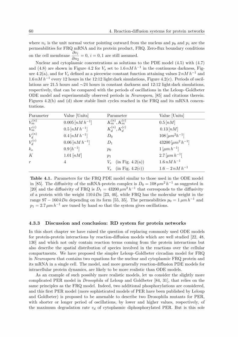
60 4. Reaction-diffusion systems for protein networks
where n1 is the unit normal vector pointing outward from the nucleus and p0 and p1 are thepermeabilities for FRQ mRNA and its protein product, FRQ. Zero-flux boundary conditions
on the cell membrane∂vi∂n2
= 0, i = 0, 1 are still assumed.
Nuclear and cytoplasmic concentrations as solutions to the PDE model (4.5) with (4.7)and (4.8) are shown in Figure 4.2 for Vs set to 1.6nM h−1 in the continuous darkness, Fig-ure 4.2(a), and for Vs defined as a piecewise constant function attaining values 2nM h−1 and1.6nM h−1 every 12 hours in the 12:12 light:dark simulations, Figure 4.2(c). Periods of oscil-lations are 21.5 hours and ∼24 hours in constant darkness and 12:12 light:dark simulations,respectively, that can be compared with the periods of oscillations in the Leloup–GoldbeterODE model and experimentally observed periods in Neurospora, [85] and citations therein.Figures 4.2(b) and (d) show stable limit cycles reached in the FRQ and its mRNA concen-trations.
Parameter Value [Units] Parameter Value [Units]
V(n)m 0.005 [nM h−1] K
(n)m ,K
(c)m 0.5 [nM ]
V(c)m 0.5 [nM h−1] K
(n)d ,K
(c)d 0.13 [nM ]
V(n)d 0.4 [nM h−1] D0 108 [µm2h−1]
V(c)d 0.06 [nM h−1] D1 43200 [µm2 h−1]
ks 0.9 [h−1] p0 1 [µmh−1]
K 1.01 [nM ] p1 2.7 [µmh−1]
r 4 Vs (in Fig. 4.2(a)) 1.6nM h−1
Vs (in Fig. 4.2(c)) 1.6− 2nM h−1
Table 4.1. Parameters for the FRQ PDE model similar to those used in the ODE modelin [85]. The diffusivity of the mRNA-protein complex is D0 = 108µm2 h−1 as suggested in[20] and the diffusivity of FRQ is D1 = 43200µm2 h−1 that corresponds to the diffusivityof a protein with the weight 110 kDa [23, 46], while FRQ has the molecular weight in therange 97 − 160 kDa depending on its form [55, 35]. The permeabilities p0 = 1µmh−1 andp1 = 2.7µmh−1 are tuned by hand so that the system gives oscillations.
4.3.3 Discussion and conclusion: RD system for protein networks
In this short chapter we have raised the question of replacing commonly used ODE modelsfor protein-protein interactions by reaction-diffusion models which are well studied [22, 48,130] and which not only contain reaction terms coming from the protein interactions butalso describe the spatial distribution of species involved in the reactions over the cellularcompartments. We have proposed the simpler Leloup–Goldbeter circadian model for FRQin Neurospora that contains two equations for the nuclear and cytoplasmic FRQ protein andits mRNA in a single cell. The model, and more generally reaction-diffusion PDE models forintracellular protein dynamics, are likely to be more realistic than ODE models.
As an example of such possibly more realistic models, let us consider the slightly morecomplicated PER model in Drosophila of Leloup and Goldbeter [84, 31], that relies on thesame principles as the FRQ model. Indeed, two additional phosphorylations are considered,and this first PER model (more sophisticated models of PER have been published by Leloupand Goldbeter) is proposed to be amenable to describe two Drosophila mutants for PER,with shorter or longer period of oscillations, by lower and higher values, respectively, ofthe maximum degradation rate vd of cytoplasmic diphosphorylated PER. But is this sole

4.3. The Leloup–Goldbeter model for the Neurospora crassa circadian clock 61
(a)
0 12 24 36 48 60 720
0.5
1
1.5
2
2.5
3
time [h]
co
nce
ntr
atio
n [
nM
]
[FRQ](n)
[FRQ](n)
+[FRQ](c)
[FRQ mRNA](n)
Vs(t)
(b)
0 0.5 1 1.5 2 2.5 30
0.5
1
1.5
2
2.5
[FRQ](n)
[FR
Q m
RN
A](n
)
(c)
0 12 24 36 48 60 720
1
2
3
4
time [h]
co
nce
ntr
atio
n [
nM
]
[FRQ](n)
[FRQ](n)
+[FRQ](c)
[FRQ mRNA](n)
Vs(t)
(d)
0 1 2 3 40
0.5
1
1.5
2
2.5
3
[FRQ](n)
[FR
Q m
RN
A](n
)
Figure 4.2. The concentrations of the nuclear FRQ, its mRNA, and the sum of the nuclearand cytoplasmic FRQ in (a) continuous darkness, Vs = 1.6nM h−1, and in (c) 12:12 light:darkcycle, Vs = 2nM h−1 and 1.6nM h−1 every 12 hours. Concentrations are solutions to thePDE model (4.5) with the Kedem–Katchalsky BC (4.7) and (4.8). Received period in (a)is 21.5 hours, in (c) 23.5 hours. Subplots in (b) and (d) show stable limit cycles of theconcentrations. The parameters used in the PDE model (4.5) are in Table 4.1. The plottedconcentrations are scaled over the total volume of the computational domain (nucleus orcytoplasm).

62 4. Reaction-diffusion systems for protein networks
Figure 4.3. 2D cell used in simulations of the Leloup–Goldbeter PDE model. The cell isrepresented by the nucleus (central zone, blue) and the cytoplasm constituted of the endoplas-mic reticulum (perinucleic annulus, red) where no translation is allowed and the translationzones (peripheral, green) denoted by χtra in (4.5). The nucleus, thus shown as an inner disc,has radius
√10µm in this case. The endoplasmic reticulum is an annulus with radii
√10µm
and 5µm. The rest of the cytoplasm is an annulus with radii 5µm and 10µm.
change of constants the best reason, in a more physiological model, for the change in periods?Could it be related to transcription of genes, to species diffusion, to translation into proteinproducts, to cytosolic/nucleic degradation, to nucleocytoplasmic transport, to the extensionof the “dead zone” around the nucleus where translation occurs (Fig. 4.3)? The samequestions can be posed when one considers p53 and drugs amenable to electively modifyspecific parts of its intracellular dynamics. This can be rendered optimally in PDE models,that are much more physiological than (rougher) ODE models since they are naturally ableto take intracellular spatial features into account including possible space heterogeneities inthe intracellular medium (not considered in the examples, apart from the above mentioneddead zone of non-translation in the cytoplasm).
We have shown how easy it is in principle to start from an ODE compartmental model,add diffusion terms - which in their simplest version are mere laplacians - and slightly modifythe representation of exchanges between the compartments to adapt them to the new set-ting, to obtain a ready-made reaction-diffusion PDE model. However, dependence on spatialpatterns, such as oscillations in concentration, on the diffusivities and the (nuclear mem-brane) permeabilities has to be better studied, with precise identification of the underlyingbiological parameters, to understand their roles properly. To obtain more realistic PDEs onecan consider effects of different viscosities of buffers on different diffusivities of molecules oradjunction of advection terms when knowledge of aided transport makes it relevant (e.g.,transport through microtubules). To support these ideas, different mobility of molecules inthe nucleus and the cytoplasm caused by limited diffusions has led to biphasic caspase acti-vation kinetics, see [153] and citations therein. In some circumstances it might be convenientto include specific spatial structures, such as position and density of ribosomes and thus tomodel gene expression more specifically [148, 6].
Note also that the oscillatory patterns are self-organised not only due to reaction events

4.3. The Leloup–Goldbeter model for the Neurospora crassa circadian clock 63
occurring in the nucleus or in the cytoplasm but that they are also tightly connected toboundary conditions on the membranes. Thus physiological delays maintained due to thesemipermeability of the nuclear membrane are more typical for PDEs than for ODEs (if onedoes not want to deal with artificial delays represented by DDEs). We examined the Kedem–Katchalsky as representing passive transport mechanisms with the difference of concentrationsat both sides of the membrane as the driving force for exchanges; however, bigger species arerather transported actively, which should be taken into account in more sophisticated modelsof nucleocytoplasmic transport [23].
The simple RD systems could be certainly considered as an alternate solution to classicalODEs which may put some light on protein signalling and will be of some help to biologists andmodellers who want to describe intracellular spatio-temporal dynamics of proteins in a faithfulyet more demanding (in terms of parameter estimation) way. Such reaction-diffusion PDEmodels are also amenable to describe spatio-temporal dynamics at the level of cell populationsand that, by introducing intercellular signalling, it is in principle possible to connect the twoobservation levels. This perspective still remains a challenge to mathematicians and modellersin biology.

64 4. Reaction-diffusion systems for protein networks

5
Reaction-diffusion model for thep53 network
Recently observed oscillatory behaviour of p53 in single cells under stress conditionsinspires several research groups in simulating and studying the dynamics of the pro-tein with the perspective of a proper understanding of physiological meanings of theoscillations. In this chapter, we propose a reaction-diffusion PDE model of p53 ac-tivation and regulation in single cells following DNA damage and we show that thep53 oscillations can be retrieved by plainly involving p53-Mdm2 and ATM-p53-Wip1negative feedbacks, which are sufficient for oscillations experimentally, with no fur-ther need to introduce any delays into the protein responses and without consideringadditional positive feedback.
Organisation of the chapter is as follows: Spatio-temporal model for p53 is introducedin Sections 5.1 and 5.2. Numerical simulations are presented in Section 5.3 and adiscussion with conclusions in Section 5.4.
Partial results presented in this chapter were published in [46],
[46] J. Elias, L. Dimitrio, J. Clairambault, and R. Natalini. The dynamics of p53in single cells: physiologically based ODE and reaction–diffusion PDE models.Physical Biology, 11(4):045001, 2014.
5.1 Rationale for a p53 PDE modelling
Let us briefly recall basic features of the dynamics of p53 which are described more ex-tensively in Chapter 1. Following DNA damage, an information signalising the presence ofDSB is transmitted to the inactive ATM dimers through an upstream signal E (begin eitherthe MRN complex or any other signal produced by the chromatin). Activated ATM thenphosphorylates p53 (on Ser15) which disrupts binding to its main regulator, the E3 ligaseMdm2, a transcription target for p53. The regulation of p53 by Mdm2 is predominantlyachieved through (multiple-)ubiquitination, followed by nuclear export of p53 and its subse-quent degradation. Such regulation by Mdm2 is possible due to previous p53 deactivation,i.e., Ser15 dephosphorylation by the phosphatase Wip1, which also dephosphorylates ATM,rendering the proteins inactive, see Figure 5.1.
The most pioneering works revealing experimentally spatio-temporal dynamics of p53 in
65

66 5. Reaction-diffusion model for the p53 network
Figure 5.1. p53 dynamics in response to DNA damage: activated ATM targets p53 forphosphorylation, which results in inhibition of the p53-Mdm2 compound formation; p53accumulates in the nucleus and acts as a transcription factor for Mdm2 and Wip1; Wip1dephosphorylates ATM and p53 keeping them inactive and enabling Mdm2 to bind p53 again,Mdm2 initiates ubiquitination of p53, its nuclear export and degradation. This dynamicsfollows two negative feedback loops: the first one between p53 and Mdm2 and the secondone between ATM and Wip1 through the intermediate p53.
single cells have been performed by the research group of Galit Lahav, see for example [15,56, 77, 91, 123, 124]. In particular, it has been shown that the negative feedbacks p53-Mdm2and ATM-p53-Wip1 are essential to maintain sustained oscillations in the p53 concentration[15], observed in the majority of cells following exposure of γ-radiation doses and other stressagents (e.g. neocarzinostatin) [77]. The p53-Mdm2 negative feedback, however, primarilyfunctions to gain homeostasis in the DDR (keeping the concentration of p53 at low levels)rather than oscillations [147], Figure 5.2. The second negative feedback, i.e. ATM-p53-Wip1,is between ATM and Wip1 with an intermediate substrate p53 (Figure 5.1). Wip1 regulatesboth ATM and p53 levels through dephosphorylation. However, since ATM is the activatorof p53 response and the ATM-dependent phosphorylation of p53 is critical for its escape fromMdm2, the inactivation of both protein by Wip1 and structural representation of cellularprocesses (e.g., gene transcription and translation) may impose time delays which could besufficient to reproduce sustained oscillations. Other mathematical models simulating p53through the p53-Mdm2 negative feedback either directly impose delays onto the equationsand thus use Delayed Differential Equations (DDEs) or involve inter-compartmental transportof species, often coupled by a positive feedback (primarily via ODEs), see the overview of theexisting models in Section 2.5.
We have shown in Chapter 3 that whenever classical Michaelis–Menten kinetics is used tomathematically describe protein reactions in a modelling setting where compartmental local-isation of cellular events nor any positive feedback is considered, the two negative feedbacksdid not produce oscillations (and eventually led to p53 homeostasis). Instead of involvingany of the observed positive feedback loops, we show that it is sufficient to distinguish be-tween cellular events occurring either in the nucleus or in the cytoplasm to obtain sustainedlyoscillating p53 concentration (due to its nuclear accumulation and nuclear clearance) that iscompatible with experimental observations. Note that different positive feedbacks may playprime roles in different phases of the p53 signalling and may depend on highly specific con-

5.2. Modelling p53 dynamics: physiological ODE and reaction-diffusion PDE models 67
ditions [60, 111], thus they should not be ruled out completely; however, none of them hasbeen reported as necessary for oscillations in [15].
Compartmental distribution of the cellular events between the nucleus (e.g., gene tran-scription, p53 activation by ATM and its deactivation by Wip1) and the cytoplasm (e.g.,mRNA translation into proteins, p53 degradation) suggests to involve spatial variables [43].Thus, based on our compartmental ODE model introduced in Chapter 3, we propose to modelthe ATM-p53-Mdm2-Wip1 protein dynamics following DNA damage (depicted in Fig. 5.3) asa 2D and 3D reaction–diffusion problem with the transmission of species between the nucleusand the cytoplasm, as we have seen in the example of the FRQ model in Chapter 4. Toour best knowledge, the only spatio-temporal p53-Mdm2 models formulated by PDEs areproposed in [43, 142]; however, they contain neither ATM nor Wip1 signalling.
cytoplasm nucleus
p53 p53
Mdm2
ub
p53ub p53ubMdm2
ub
ATMATM
1.
2. 2.
Figure 5.2. p53 dynamics in a normal unstressed cell: 1. The protein ATM in its inactiveform is dimerised, unable to phosphorylate p53, which subsequently cannot act as a transcrip-tion factor. p53 is assumed to freely migrate between the compartments, Mdm2 moves fromthe translation sites to the nucleus. Mdm2-ubiquitin dependent degradation in the nucleus,2., and in the cytoplasm, 3., retains the concentration of p53 at low levels in the compart-ments (mainly in the nucleus). Dashed arrows indicate directions of molecule migrations,uni- or bidirectional, T-shaped lines meaning impossible nucleocytoplasmic transport in theT-end direction; solid arrows show schematically reactions in the signalling pathways. Reddashed T-shaped line shows inhibition of ATM-dependent phosphorylation of p53.
5.2 Modelling p53 dynamics: physiological ODE andreaction-diffusion PDE models
5.2.1 Mathematical formalism and notation
A simplified cell model consists of two compartments, the nucleus Ω1 and the cytoplasm Ω2
with the nuclear membrane Γ1 and the cellular membrane Γ2, as it is schematically shownon Figure 4.1.
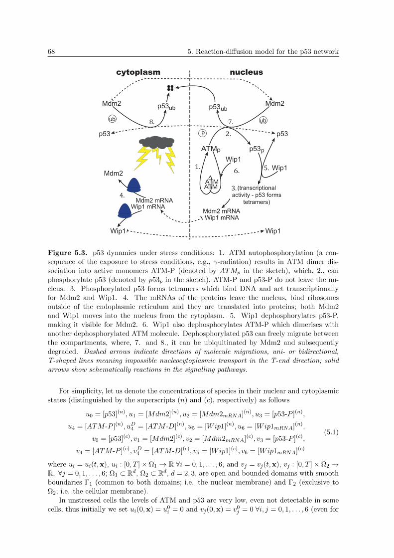
68 5. Reaction-diffusion model for the p53 network
cytoplasm nucleus
p53 p53
Mdm2 p53ub p53ubMdm2
ub
p
p53p
(transcriptionalactivity - p53 forms
tetramers)
pATM
Wip1
Wip1 mRNAMdm2 mRNA
Wip1 mRNAMdm2 mRNA
Mdm2
Wip1 Wip1
Wip1
ATMATM
1.
2.
3.4.
5.6.
8. 7.ub
Figure 5.3. p53 dynamics under stress conditions: 1. ATM autophosphorylation (a con-sequence of the exposure to stress conditions, e.g., γ-radiation) results in ATM dimer dis-sociation into active monomers ATM-P (denoted by ATMp in the sketch), which, 2., canphosphorylate p53 (denoted by p53p in the sketch), ATM-P and p53-P do not leave the nu-cleus. 3. Phosphorylated p53 forms tetramers which bind DNA and act transcriptionallyfor Mdm2 and Wip1. 4. The mRNAs of the proteins leave the nucleus, bind ribosomesoutside of the endoplasmic reticulum and they are translated into proteins; both Mdm2and Wip1 moves into the nucleus from the cytoplasm. 5. Wip1 dephosphorylates p53-P,making it visible for Mdm2. 6. Wip1 also dephosphorylates ATM-P which dimerises withanother dephosphorylated ATM molecule. Dephosphorylated p53 can freely migrate betweenthe compartments, where, 7. and 8., it can be ubiquitinated by Mdm2 and subsequentlydegraded. Dashed arrows indicate directions of molecule migrations, uni- or bidirectional,T-shaped lines meaning impossible nucleocytoplasmic transport in the T-end direction; solidarrows show schematically reactions in the signalling pathways.
For simplicity, let us denote the concentrations of species in their nuclear and cytoplasmicstates (distinguished by the superscripts (n) and (c), respectively) as follows
u0 = [p53](n), u1 = [Mdm2](n), u2 = [Mdm2mRNA](n), u3 = [p53-P ](n),
u4 = [ATM -P ](n), uD4 = [ATM -D](n), u5 = [Wip1](n), u6 = [Wip1mRNA](n),
v0 = [p53](c), v1 = [Mdm2](c), v2 = [Mdm2mRNA](c), v3 = [p53-P ](c),
v4 = [ATM -P ](c), vD4 = [ATM -D](c), v5 = [Wip1](c), v6 = [Wip1mRNA](c)
(5.1)
where ui = ui(t,x), ui : [0, T ]× Ω1 → R ∀i = 0, 1, . . . , 6, and vj = vj(t,x), vj : [0, T ]× Ω2 →R, ∀j = 0, 1, . . . , 6; Ω1 ⊂ Rd, Ω2 ⊂ Rd, d = 2, 3, are open and bounded domains with smoothboundaries Γ1 (common to both domains; i.e. the nuclear membrane) and Γ2 (exclusive toΩ2; i.e. the cellular membrane).
In unstressed cells the levels of ATM and p53 are very low, even not detectable in somecells, thus initially we set ui(0,x) = u0
i = 0 and vj(0,x) = v0j = 0 ∀i, j = 0, 1, . . . , 6 (even for

5.2. Modelling p53 dynamics: physiological ODE and reaction-diffusion PDE models 69
Mdm2 which can be presented in cells keeping p53 at low concentrations). Reaction termsof the considered reactions, transmission conditions through Γ1 and boundary conditions onΓ2 are specified in the following sections. Note that, although based on our assumptions wehave v3 = 0, v4 = 0 and vD4 = 0, we will involve these species in the equations to make overallnotation easier to follow.
5.2.2 Compartmental ODE model
The physiological ODE model for the dynamics of p53 network is developed and examinedin Chapter 3. This compartmental ODE model consists of equations (3.16) and (3.17).The transmission conditions through Γ1 are expressed as differences of the concentrationsof species in both compartments controlled by the permeability coefficients and a specialvolume ratio Vr due to different velocities of reactions occurring either in the nucleus or inthe cytoplasm [28].
Let us write u = (u0, u1, . . . , u6)T and v = (v0, v1, . . . , v6)T for the concentrations ofspecies and f = (f0, f1, . . . , f6])T , fi = fi(u,v), and g = (g0, g1, . . . , g6)T , gi = gi(u,v),i = 0, . . . , 6, for the reaction terms rising from the LMA, Michaelis-Menten and Hill kineticsand the transmission-like terms, i.e. the terms standing on the right-hand side of the ODEequations in (3.16) and (3.17). Thus, we can write equations for the compartmental ODEsetting as a coupled system
du
dt= f(u,v) and
dv
dt= g(u,v) (5.2)
with the initial conditions u(0) = u0 = 0 and v(0) = v0 = 0.
5.2.3 Reaction-diffusion PDE model
Based on the ODE model (5.2), by adding a diffusion term in each equation we can formulate areaction–diffusion model describing the evolution of the concentrations of proteins as functionsof time and space in a cell composed of the two compartments, Figure 4.1. The dynamics ofthe proteins including directions of their migration through the nuclear membrane is discussedin the biological overview and it is schematically shown on Figure 5.3.
The reaction–diffusion model for the nuclear and cytoplasmic concentrations u(t,x) =(u0, . . . , u6)T (t,x) and v(t,x) = (v0, . . . , v6)T (t,x), respectively, can be written (in the vectorform) by
∂u
∂t− div(D∇u) = rΩ1(u) on (0, T )× Ω1, (5.3)
and∂v
∂t− div(D∇v) = rΩ2(v) on (0, T )× Ω2, (5.4)
with the initial conditions u(0,x) = u0 = 0 and v(0,x) = v0 = 0 and boundary conditionson Γ1 and Γ2 specified in the next section. In (5.3) and (5.4), D is a diagonal matrix withthe diffusion coefficients on the diagonal (Table 5.2), which are equal for both compartments;and rΩi
, i = 1, 2, store the (nonlinear) reaction and production/degradation terms. The p53basal production rate and the terms related to the translation of the mRNAs into the proteinsare multiplied by the characteristic functions χC and χCD defining areas of the cytoplasmwhere the protein production events occur. These functions are defined and illustrated onFigure 5.4 in Section 5.2.7, see also Figure 2.2.

70 5. Reaction-diffusion model for the p53 network
The corresponding equations of the RD system (5.3) and (5.4), are as follows:
(N)
∂u0
∂t= Dp53∆u0 + kdph1u5
u3
Kdph1 + u3− kubu1
u0
Kub + u0− kph1u4
u0
Kph1 + u0
∂u1
∂t= Dmdm2∆u1 − δmdm2u1
∂u2
∂t= DmRNA∆u2 + kSm + kSpm
(u0 + u3)4
K4Spm
+ (u0 + u3)4− δmRNAu2
∂u3
∂t= Dp53∆u3 + kph1u4
u0
Kph1 + u0− kdph1u5
u3
Kdph1 + u3
∂u4
∂t= DATM∆u4 + 2kph2u
D4
E2
K2ph2 + E2
− kdph2u5u4
Kdph2 + u4
∂uD4∂t
= DATM∆uD4 − kph2uD4
E2
K2ph2 + E2
+1
2kdph2u5
u4
Kdph2 + u4
∂u5
∂t= Dwip1∆u5 − δwip1u5
∂u6
∂t= DwRNA∆u6 + kSw + kSpw
(u0 + u3)4
K4Spw
+ (u0 + u3)4− δwRNAu6
(5.5)
(C)
∂v0
∂t= Dp53∆v0 + kSχC − kubv1
v0
Kub + v0− δp53v0
∂v1
∂t= Dmdm2∆v1 + ktmv2χCD − δmdm2v1
∂v2
∂t= DmRNA∆v2 − δmRNAv2
∂v3
∂t= Dp53∆v3
∂v4
∂t= DATM∆v4
∂vD4∂t
= DATM∆vD4
∂v5
∂t= Dwip1∆v5 + ktwv6χCD − δwip1v5
∂v6
∂t= DwRNA∆v6 − δwRNAv6
(5.6)
Note that there are some differences between the ODE and PDE models. In particular,we consider both equations for the monomeric u4, v4 and dimeric uD4 , vD4 forms of ATM bothdiffusing with the same diffusion rate DATM (but still satisfying the conservation law:
´u4 +
2uD4 dx = const = ATMTOT ), see discussion in Section 2.2.1. In addition, the Hill functionwith the coefficient 2 is used for ATM activation by E and ATM-P dephosphorylation by
Wip1 is modelled as a simple enzyme reaction ATM -P+Wip1 Ckdph2−→ “1
2ATM -D”+Wip1when compared to (3.3). Then the equations for the mRNAs v2 and v6 represent the evolutionof the total amount of the mRNA and not the free mRNA molecules considered in the ODEmodel. Mdm2 is assumed to move from the cytoplasm to nucleus only, as its main functionis to remove p53 from the DNA sites. Finally, we assume that both p53 and p53-P appearin the transcription process for its substrate genes1.
1In the ODE model we assumed that only p53-P, which is hidden from Mdm2, is able to form tetramers

5.2. Modelling p53 dynamics: physiological ODE and reaction-diffusion PDE models 71
All the kinetic parameters used in simulations are shown in Table 5.5, permeabilities(translocation) and diffusion coefficients in Table 5.2.
5.2.4 Nucleocytoplasmic transmission BC: Kedem–Katchalsky boundaryconditions
Boundary conditions applied for a passive transmission of the species through the nuclearmembrane are discussed in Section 2.4. Let us recall that a driving force for the diffusivetransport in the Kedem–Katchalsky BC is the difference in concentrations at both sides of themembrane, which is the simplification of a more realistic driving force standing behind most ofthe passive transport processes — a chemical potential gradient — which depends not only onconcentrations but also on pressure, temperature, electric field and other quantities. The sameBC can be derived easily from Fick’s first law for stationary fluids (i.e. with no net movement,no bulk motion and no coupling effect of more cargoes transported simultaneously); see alsoFigure 2.3.
In particular, a contribution to the overall concentration (increase or decrease) of a chem-ical with the nuclear concentration ui, for some i, throughout Γ1 is defined by
−Di∂ui∂n1
= −pi(vi − ui). (5.7)
where vi is the cytoplasmic concentration of the same chemical, pi is the permeability. Equa-tion (5.7) says that the flux (LHS of (5.7)) is equal to the difference of the concentrationsacross the nuclear membrane for the direction of flow from ui to vi if ui > vi, and the otherway round if ui < vi, which is in agreement with the assumption for the particle flow (Fick’sfirst law) to be directed from a compartment with higher concentration of the chemical to acompartment with its smaller concentration.
Similar condition, particularly,
Di∂vi∂n1
= −pi(ui − vi), (5.8)
is written for the cytoplasmic concentration of the chemical, however, with the minus signbecause of the orientation of the normal vector n1 which points outward from the nucleus Ω1
to the cytoplasm Ω2, see Figure 4.1.The Kedem–Katchalsky BC (5.7) and (5.8) satisfy the continuity of the flux condition on
the boundary (what goes out from one compartment must come in to the second compart-ment),
Di∂ui∂n1
= Di∂vi∂n1
, (5.9)
however, usually, ui 6= vi on both sides of the nuclear membrane because of the permeabil-ity of the nuclear membrane (non-zero membrane “conductance”). In contrast, continuoustranslocation of species throughout the nuclear membrane modelled by the transmission con-ditions ui = vi together with (5.9) are considered in [142] (i.e. no limits on perviousness ofthe membrane are taken into account in [142]).
Equations (5.7) and (5.8) are applied to the chemicals which migrate between Ω1 andΩ2 (i.e., the protein p53). Other particular cases when a chemical translocates from onecompartment to another in one direction only, e.g. Mdm2 and Wip1 mRNAs which movefrom the nucleus to the cytoplasm and not back, and the proteins Mdm2 and Wip1, that
and bind the DNA. However, the phosphorylation status of p53 does not likely determine tetramerisation ofp53. In fact, tetramerisation represents another mechanism how p53 can escape from Mdm2.

72 5. Reaction-diffusion model for the p53 network
Chemical nuclear changes cytoplasmic changes
p53 −Dp53∂u0
∂n1= −pp53(v0 − u0) Dp53
∂v0
∂n1= −pp53(u0 − v0)
Mdm2 −Dmdm2∂u1
∂n1= −pmdm2(v1 − u1) Dmdm2
∂v1
∂n1= −pmdm2(u1 − v1)
Mdm2 mRNA −DmRNA∂u2
∂n1= pmRNAu2 DmRNA
∂v2
∂n1= −pmRNAu2
p53-P −Dp53∂u3
∂n1= 0 Dp53
∂v3
∂n1= 0
ATM-P −DATM∂u4
∂n1= 0 DATM
∂v4
∂n1= 0
ATM-D −DATM∂uD4∂n1
= 0 DATM∂vD4∂n1
= 0
Wip1 −Dwip1∂u5
∂n1= −pwip1v5 Dwip1
∂v5
∂n1= pwip1v5
Wip1 mRNA −DwRNA∂u6
∂n1= pwRNAu6 DwRNA
∂v6
∂n1= −pwRNAu6
Table 5.1. The Kedem–Katchalsky transmission boundary conditions on Γ1 with thediffusion coefficients Di and the translocation (permeability) rates pi for each specie i ∈p35,mdm2,mRNA,ATM,wip1, wRNA.
move from the cytoplasm to the nucleus, and, finally, the cases of ATM and phosphorylatedp53-P, which do not leave the nucleus, are simple modifications of (5.7) and (5.8) and arelisted in Table 5.1.
In the vector form, the Kedem–Katchalsky BC can be uniquely written by
−D ∂u
∂n1= PgΩ1(u,v) and D
∂v
∂n1= PgΩ2(u,v), (5.10)
where D and P are diagonal matrices with the diffusion and permeability coefficients on thediagonals, and gΩ1 = gΩ1(u,v) and gΩ2 = gΩ2(u,v) collect the terms on the right hand sidesof the boundary conditions as they are stated in Table 5.1; note that gΩ1 = −gΩ2 .
Finally, we do not assume exchange of the species between cells. Thus, we set
D∂v
∂n2= 0 (5.11)
on the cell membrane, where n2 is the normal vector pointed outward from the cell membrane.
5.2.5 Diffusion and permeability coefficients for the RD model
Transport of the species through the nuclear membrane Γ1 is determined by the diffusionand the permeability coefficients in (5.10). All the permeability and diffusion coefficientsconsidered in our simulations are listed in Table 5.2. Note that due to the similar nuclearand cytoplasmic cytosol viscosity we will consider the same diffusion values for both compart-ments. Note also that there are other possibilities how to approximate diffusion coefficients ofproteins, for example, by using Einstein’s formula [23] which, however, requires Stokes radiiof the proteins, which are often not known.

5.2. Modelling p53 dynamics: physiological ODE and reaction-diffusion PDE models 73
Chemical Diffusion [µm2/min] Permeability [µm/min] Weight [kDa]
GFP — 2500 [64, 65] — — 26.9 [64]
p53-GFP — 900 [64, 65] — — ∼80 [64]
p53 (dimer) Dp53 1000 [64, 65] pp53 1 [est.] 53 [158]
Mdm2 Dmdm2 1000 [est.] pmdm2 1 [est.] 90 [109, 154]
Mdm2 mRNP DmRNA 1.8 [20] pmRNA 0.1 [est.] ≤1600 [34]
p53-P (dimer) Dp53 1000 [64, 65] pp53-P 0 53 [158]
ATM (monomer) DATM 300 [est.] pATM 0 370 [7]
Wip1 Dwip1 1000 [est.] pwip1 1 [est.] 61 [52]
Wip1 mRNP DwRNA 1.8 [20, 146] pwRNA 0.1 [est.] ≤1600 [34]
Table 5.2. (Estimated) diffusion and translocation (permeability) coefficients used in thePDE model. We assume that p53-P and ATM-P do not leave nor enter the nucleus. Althoughwe consider ATM in its monomer and dimer we assume that both conformations diffuse withthe same diffusion rate. Similarly, we assume that the diffusivity for p53 and p53-P is thesame. The diffusion rates could be roughly estimated by comparison of the known diffusionsand the molecular weights of the species. Due to the lack of data on permeabilities, we haverun several simulations and tested various permeability rates for which oscillations appear.In this table are those rates we have chosen as the reference ones. Note that in the ODEmodel proposed in Chapter 3 we considered different permeabilities than in the PDE model.
5.2.6 Nondimensionalisation
The PDE system (5.3) and (5.4), more precisely equations (5.5) and (5.6)) with the Kedem–Katchalsky BC (5.10) explicitly listed in Tables 5.1 and with the parameters in Tables 5.5 and5.2, are nondimensionalised before they are solved. See [132] for more details on advantagesand the necessity of nondimensionalisation.
For the reference concentration αi, i = 0, . . . , 7, the scaled nuclear and cytoplasmic con-centrations of the species are defined by, respectively,
ui =uiαi
and vi =viαi. (5.12)
By setting
t =t
τ, xj =
xjL, j = 1, . . . , d (5.13)
and
kdph1 = τkdph1(α5/α0), Kdph1 = Kdph1/α3, kph1 = τkph1(α4/α0),
Kph1 = Kph1/α0, kub = τkub(α1/α0), Kub = Kub/α0,
δp53 = τδp53, δmdm2 = τδmdm2, δmRNA = τδmRNA, δwip1 = τδwip1, δwRNA = τδwRNA,
kSm = τkSm/α2, kSpm = τkSpm/α2, KSpm = KSpm/α3,
kSw = τkSw/α6, kSpw = τkSpw/α6, KSpw = KSpw/α3,
kdph2 = τkdph2(α5/α4), Kdph2 = Kdph2/α24, kph2 = τkph2, Kph2 = Kph2/α4
kS = τkS/α0, ktm = τktm, ktw = τktw, E = E/α4,
pi = τpi/L, Di = τDi/L2 ∀i,
(5.14)
we finally arrive at the systems used in our simulations. The nondimensionalised equations

74 5. Reaction-diffusion model for the p53 network
of the PDE model are not shown here, since they are very similar to the nonscaled equationsexcept for the entries replaced by their nondimensionalised substitutions.
We have chosen τ = 1min, αi = 1µM for each i and L = 10µm in the followingsimulations2.
5.2.7 Numerical simulations of PDEs in 2 and 3 dimensions
The nondimensionalised reaction–diffusion problem derived from (5.3) and (5.4) with thezero initial conditions and the Kedem–Katchalsky BC (5.10) is solved numerically in 2 and3 dimensions on the triangulations shown on Figure 5.4 by the semi-implicit Rothe method,see Appendix B and, e.g., [130], implemented in the FreeFem++ solver [62]. The cell underconsideration on Figure 5.4 has radius equal to 1 length unit, thus, by considering the scalinglength L = 10µm, the cell model represents a real cell with size 20µm in diameter3.
Figure 5.4. The 2D and 3D cell is represented by a disc and by a 3D ball, respectively, withradius 10µm. The nucleus, A, is shown as an inner disc and an inner ball, respectively, withradius 3µm. The endoplasmic reticulum B, where no production of the proteins occurs, isan annulus with radii 3µm and 5µm; the ring-shaped area C, where the basal production ofp53 is assumed to occur, is an annulus with radii 5 and 6µm, respectively, and the rest of thecytoplasm, D, is an annulus with radii 6 and 10µm. Translation of the mRNAs is supposedto occur in C+D. The 2D and 3D cell triangulations are generated by FreeFem++, [62].
As already mentioned in Section 2.2, the total net production of p53 determined by thebasal production rate kS is restricted to a narrow ring-shaped area within the cytoplasm(denoted by C on Figure 5.4) separated from the nucleus by the endoplasmic reticulum (ER,denoted by B on Figure 5.4). Numerically, we multiply kS by the characteristic function
2Other choices for the reference concentrations can be obviously chosen, for instance, such that someunknown parameters are eliminated, in our particular case we nevertheless use all the reference concentrationsto be equal to each other; we used different reference concentrations αi for different species i in [46].
3Note that a diameter of an average eukaryotic cell is between 10 − 20µm and a diameter of the nucleusranges from 3−10µm [105]. The cell under our consideration is of a diameter 20µm with the nucleus of 6µmin diameter.
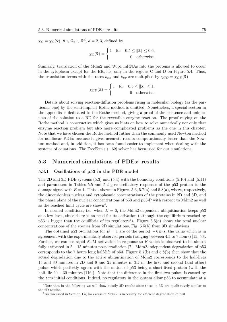
5.3. Numerical simulations of PDEs: results 75
χC = χC(x), x ∈ Ω2 ⊂ Rd, d = 2, 3, defined by
χC(x) =
1 for 0.5 ≤ ‖x‖ ≤ 0.6,
0 otherwise.
Similarly, translation of the Mdm2 and Wip1 mRNAs into the proteins is allowed to occurin the cytoplasm except for the ER, i.e. only in the regions C and D on Figure 5.4. Thus,the translation terms with the rates ktm and ktw are multiplied by χCD = χCD(x)
χCD(x) =
1 for 0.5 ≤ ‖x‖ ≤ 1,
0 otherwise.
Details about solving reaction-diffusion problems rising in molecular biology (as the par-ticular one) by the semi-implicit Rothe method is omitted. Nonetheless, a special section inthe appendix is dedicated to the Rothe method, giving a proof of the existence and unique-ness of the solution to a RD for the reversible enzyme reaction. The proof relying on theRothe method is constructive which gives us hints on how to solve numerically not only thatenzyme reaction problem but also more complicated problems as the one in this chapter.Note that we have chosen the Rothe method rather than the commonly used Newton methodfor nonlinear PDEs because it gives accurate results computationally faster than the New-ton method and, in addition, it has been found easier to implement when dealing with thesystems of equations. The FreeFem++ [62] solver has been used for our simulations.
5.3 Numerical simulations of PDEs: results
5.3.1 Oscillations of p53 in the PDE model
The 2D and 3D PDE systems (5.3) and (5.4) with the boundary conditions (5.10) and (5.11)and parameters in Tables 5.5 and 5.2 give oscillatory responses of the p53 protein to thedamage signal with E = 1. This is shown in Figures 5.6, 5.7(a) and 5.8(a), where, respectively,the dimensionless nuclear and cytoplasmic concentrations of the proteins in 2D and 3D, andthe phase plane of the nuclear concentrations of p53 and p53-P with respect to Mdm2 as wellas the reached limit cycle are shown4.
In normal conditions, i.e. when E = 0, the Mdm2-dependent ubiquitination keeps p53at a low level, since there is no need for its activation (although the equilibrium reached byp53 is bigger than the equilibria of its regulators5). Figure 5.5(a) shows the total nuclearconcentrations of the species from 2D simulations, Fig. 5.5(b) from 3D simulations.
The obtained p53 oscillations for E = 1 are of the period ∼ 6hrs, the value which is inagreement with the experimentally observed periods (ranging between 4.5 to 7 hours) [15, 56].Further, we can see rapid ATM activation in response to E which is observed to be almostfully activated in 5− 15 minutes post-irradiation [7]. Mdm2-independent degradation of p53corresponds to the 7 hours long half-life of p53. Figure 5.7(b) and 5.8(b) then show that theactual degradation due to the active ubiquitination of Mdm2 corresponds to the half-lives15 and 30 minutes in 2D and 8 and 25 minutes in 3D in the first and second (and other)pulses which perfectly agrees with the notion of p53 being a short-lived protein (with thehalf-life 20 − 30 minutes [116]). Note that the difference in the first two pulses is caused bythe zero initial conditions. Indeed, no regulators in the system allow p53 to accumulate at a
4Note that in the following we will show mostly 2D results since those in 3D are qualitatively similar tothe 2D results.
5As discussed in Section 1.5, no excess of Mdm2 is necessary for efficient degradation of p53.
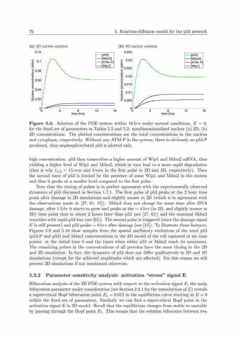
76 5. Reaction-diffusion model for the p53 network
(a) 2D nuclear solution
0 4 8 12 160
0.02
0.04
0.06
0.08
0.1
0.12
time (hrs)
Nucle
ar
concentr
ations (
adim
)
[p53]
[Mdm2]
[ATM−P]
[Wip1]
(b) 3D nuclear solution
0 4 8 12 160
0.005
0.01
0.015
0.02
0.025
0.03
0.035
time (hrs)
Nucle
ar
concentr
ations (
adim
)
[p53]
[Mdm2]
[ATM−P]
[Wip1]
Figure 5.5. Solution of the PDE system within 16hrs under normal conditions, E = 0,for the fixed set of parameters in Tables 5.5 and 5.2: nondimensionalised nuclear (a) 2D, (b)3D concentrations. The plotted concentrations are the total concentrations in the nucleusand cytoplasm, respectively. Without any ATM-P in the system, there is obviously no p53-Pproduced, thus unphosphorylated p53 is plotted only.
high concentration. p53 then transcribes a higher amount of Wip1 and Mdm2 mRNA, thusyielding a higher level of Wip1 and Mdm2, which in turn lead to a more rapid degradation(that is why t1/2 = 15min and 8min in the first pulse in 2D and 3D, respectively). Thenthe second wave of p53 is limited by the presence of some Wip1 and Mdm2 in the systemand thus it peaks at a smaller level compared to the first pulse.
Note that the timing of pulses is in perfect agreement with the experimentally observeddynamics of p53 discussed in Section 1.7.1. The first pulse of p53 peaks at the 2 hour timepoint after damage in 2D simulations and slightly sooner in 3D (which is in agreement withthe observations made in [27, 61, 15]). Mdm2 does not change for some time after DNAdamage, after 1.5hr it starts to grow and peaks at the ∼ 4hrs (in 2D, and slightly sooner in3D) time point thus in about 2 hours later than p53 (see [27, 61]) and the maximal Mdm2coincides with rapid p53 loss (see [61]). The second pulse is triggered (since the damage signalE is still present) and p53 peaks ∼ 8hrs after damage (see [15]). To illustrate these features,Figures 5.9 and 5.10 show samples from the spatial oscillatory evolutions of the total p53(p53-P and p53) and Mdm2 concentrations in the 3D model of the cell captured at six timepoints: at the initial time 0 and the times when either p53 or Mdm2 reach its maximum.The remaining pulses in the concentrations of all proteins have the same timing in the 2Dand 3D simulation. In fact, the dynamics of p53 does not differ qualitatively in 2D and 3Dsimulations (except for the achieved amplitudes which are affected). For this reason we willpresent 2D simulations if not mentioned otherwise.
5.3.2 Parameter sensitivity analysis: activation “stress” signal E
Bifurcation analysis of the 2D PDE system with respect to the activation signal E, the mainbifurcation parameter under consideration (see Section 2.2.1 for the introduction of E) revealsa supercritical Hopf bifurcation point E1 = 0.015 in the equilibrium curve starting at E = 0within the fixed set of parameters. Similarly we can find a supercritical Hopf point in theactivation signal E in 3D model. Recall that the equilibrium changes from stable to unstableby passing through the Hopf point E1. This means that the solution bifurcates between two
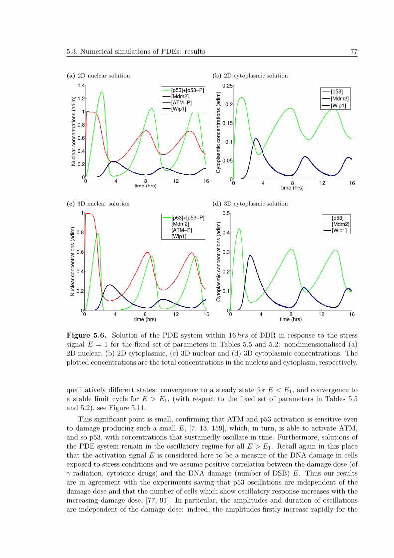
5.3. Numerical simulations of PDEs: results 77
(a) 2D nuclear solution
0 4 8 12 160
0.2
0.4
0.6
0.8
1
1.2
1.4
time (hrs)
Nucle
ar
concentr
ations (
adim
)
[p53]+[p53−P]
[Mdm2]
[ATM−P]
[Wip1]
(b) 2D cytoplasmic solution
0 4 8 12 160
0.05
0.1
0.15
0.2
0.25
time (hrs)
Cyto
pla
sm
ic c
on
ce
ntr
atio
ns (
ad
im)
[p53]
[Mdm2]
[Wip1]
(c) 3D nuclear solution
0 4 8 12 160
0.2
0.4
0.6
0.8
1
time (hrs)
Nucle
ar
concentr
ations (
adim
)
[p53]+[p53−P]
[Mdm2]
[ATM−P]
[Wip1]
(d) 3D cytoplasmic solution
0 4 8 12 160
0.1
0.2
0.3
0.4
0.5
time (hrs)
Cyto
pla
sm
ic c
oncentr
ations (
adim
)
[p53][Mdm2][Wip1]
Figure 5.6. Solution of the PDE system within 16hrs of DDR in response to the stresssignal E = 1 for the fixed set of parameters in Tables 5.5 and 5.2: nondimensionalised (a)2D nuclear, (b) 2D cytoplasmic, (c) 3D nuclear and (d) 3D cytoplasmic concentrations. Theplotted concentrations are the total concentrations in the nucleus and cytoplasm, respectively.
qualitatively different states: convergence to a steady state for E < E1, and convergence toa stable limit cycle for E > E1, (with respect to the fixed set of parameters in Tables 5.5and 5.2), see Figure 5.11.
This significant point is small, confirming that ATM and p53 activation is sensitive evento damage producing such a small E, [7, 13, 159], which, in turn, is able to activate ATM,and so p53, with concentrations that sustainedly oscillate in time. Furthermore, solutions ofthe PDE system remain in the oscillatory regime for all E > E1. Recall again in this placethat the activation signal E is considered here to be a measure of the DNA damage in cellsexposed to stress conditions and we assume positive correlation between the damage dose (ofγ-radiation, cytotoxic drugs) and the DNA damage (number of DSB) E. Thus our resultsare in agreement with the experiments saying that p53 oscillations are independent of thedamage dose and that the number of cells which show oscillatory response increases with theincreasing damage dose, [77, 91]. In particular, the amplitudes and duration of oscillationsare independent of the damage dose: indeed, the amplitudes firstly increase rapidly for the

78 5. Reaction-diffusion model for the p53 network
(a)
0 0.5 1 1.50
0.05
0.1
0.15
0.2
0.25
Nuclear [p53]+[p53−P]
Nucle
ar
[Mdm
2]
(b)
0 5 10 150
0.5
1
1.5
time (hrs)
co
nce
ntr
atio
n (
ad
im)
Total [p53]t1/2
= 15 min
t1/2
= 30 min
Figure 5.7. Solution of the 2D PDE system for the fixed set of parameters in Tables 5.5and 5.2: (a) phase portrait of dimensionless nuclear concentrations of p53 (p53 and p53-P)with respect to Mdm2; (b) decay of the total (nuclear and cytoplasmic) p53 concentration inthe cell with wt Mdm2 corresponds to the half-life of 15 and 30 minutes, respectively, in thefirst and the second pulse.
(a)
0 0.2 0.4 0.6 0.80
0.05
0.1
0.15
0.2
0.25
Nuclear [p53]+[p53−P]
Nucle
ar
[Mdm
2]
(b)
0 5 10 150
0.2
0.4
0.6
0.8
1
1.2
1.4
time (hrs)
concentr
ation (
adim
)
Total [p53]t1/2
= 8 min
t1/2
= 25 min
Figure 5.8. Solution of the 3D PDE system for the fixed set of parameters in Tables 5.5and 5.2: (a) phase portrait of dimensionless nuclear concentrations of p53 (p53 and p53-P)with respect to Mdm2; (b) decay of the total (nuclear and cytoplasmic) p53 concentration inthe cell with wt Mdm2 corresponds to the half-life of 8 and 25 minutes, respectively, in thefirst and the second pulse.

5.3. Numerical simulations of PDEs: results 79
(a) 0 h (b) 1.8 h (c) 3.5 h
(d) 8.5 h (e) 10.4 h (f) 14.2 h
Figure 5.9. 3D visualisation of the solution of the PDE system for the fixed set of parametersin Tables 5.5 and 5.2: nondimensionalised concentration of p53 (p53-P and p53). The chosensamples are captured at the times when p53 and Mdm2 reach peaks in their concentrations.
(a) 0 h (b) 1.8 h (c) 3.5 h
(d) 8.5 h (e) 10.4 h (f) 14.2 h
Figure 5.10. 3D visualisation of the solution of the PDE system for the fixed set of param-eters in Tables 5.5 and 5.2: nondimensionalised concentration of Mdm2. The chosen samplesare captured at the times when p53 and Mdm2 reach peaks in their in concentrations.
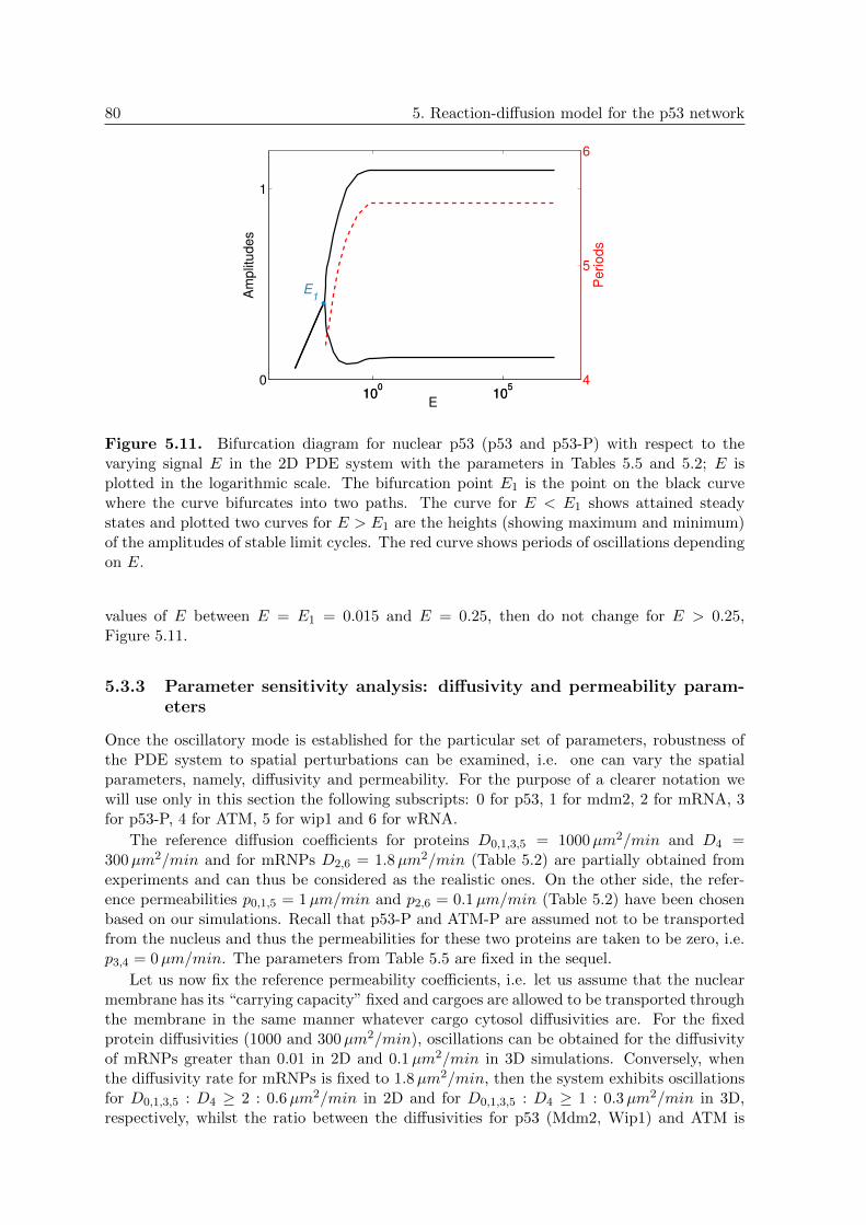
80 5. Reaction-diffusion model for the p53 network
100
105
0
1
E
Am
plit
udes
100
105
4
5
6
Periods
E1
Figure 5.11. Bifurcation diagram for nuclear p53 (p53 and p53-P) with respect to thevarying signal E in the 2D PDE system with the parameters in Tables 5.5 and 5.2; E isplotted in the logarithmic scale. The bifurcation point E1 is the point on the black curvewhere the curve bifurcates into two paths. The curve for E < E1 shows attained steadystates and plotted two curves for E > E1 are the heights (showing maximum and minimum)of the amplitudes of stable limit cycles. The red curve shows periods of oscillations dependingon E.
values of E between E = E1 = 0.015 and E = 0.25, then do not change for E > 0.25,Figure 5.11.
5.3.3 Parameter sensitivity analysis: diffusivity and permeability param-eters
Once the oscillatory mode is established for the particular set of parameters, robustness ofthe PDE system to spatial perturbations can be examined, i.e. one can vary the spatialparameters, namely, diffusivity and permeability. For the purpose of a clearer notation wewill use only in this section the following subscripts: 0 for p53, 1 for mdm2, 2 for mRNA, 3for p53-P, 4 for ATM, 5 for wip1 and 6 for wRNA.
The reference diffusion coefficients for proteins D0,1,3,5 = 1000µm2/min and D4 =300µm2/min and for mRNPs D2,6 = 1.8µm2/min (Table 5.2) are partially obtained fromexperiments and can thus be considered as the realistic ones. On the other side, the refer-ence permeabilities p0,1,5 = 1µm/min and p2,6 = 0.1µm/min (Table 5.2) have been chosenbased on our simulations. Recall that p53-P and ATM-P are assumed not to be transportedfrom the nucleus and thus the permeabilities for these two proteins are taken to be zero, i.e.p3,4 = 0µm/min. The parameters from Table 5.5 are fixed in the sequel.
Let us now fix the reference permeability coefficients, i.e. let us assume that the nuclearmembrane has its “carrying capacity” fixed and cargoes are allowed to be transported throughthe membrane in the same manner whatever cargo cytosol diffusivities are. For the fixedprotein diffusivities (1000 and 300µm2/min), oscillations can be obtained for the diffusivityof mRNPs greater than 0.01 in 2D and 0.1µm2/min in 3D simulations. Conversely, whenthe diffusivity rate for mRNPs is fixed to 1.8µm2/min, then the system exhibits oscillationsfor D0,1,3,5 : D4 ≥ 2 : 0.6µm2/min in 2D and for D0,1,3,5 : D4 ≥ 1 : 0.3µm2/min in 3D,respectively, whilst the ratio between the diffusivities for p53 (Mdm2, Wip1) and ATM is

5.3. Numerical simulations of PDEs: results 81
Diffusion values for oscillations Description Dim.
0.01 ≤ D2,6 D0,1,3,5 = 1000, D4 = 300 fixed 2D
2 : 0.6 ≤ D0,1,3,5 : D4 ratio D0,1,3,5 : D4 and D2,6 = 1.8 fixed 2D
1 : 0.3 : 0.0018 ≤ D0,1,3,5 : D4 : D2,6 ratio D0,1,3,5 : D4 : D2,6 fixed 2D
0.1 ≤ D2,6 D0,1,3,5 = 1000, D4 = 300 fixed 3D
1 : 0.3 ≤ D0,1,3,5 : D4 ratio D0,1,3,5 : D4 and D2,6 = 1.8 fixed 3D
5 : 1.5 : 0.009 ≤ D0,1,3,5 : D4 : D2,6 ratio D0,1,3,5 : D4 : D2,6 fixed 3D
Table 5.3. Ranges for the diffusion parameters (in µm2/min) for which the 2D and 3D PDEsystems give oscillations, assuming that the considered ratios and the unmentioned parame-ters from Tables 5.5 and 5.2 are fixed. As for the reference values, D0,1,3,5 = 1000, D4 = 300and D2,6 = 1.8µm2/min for the p53 (Mdm2, Wip1), ATM and mRNPs, respectively, havebeen taken. Subscripts: 0 for p53, 1 for mdm2, 2 for mRNA, 3 for p53-P, 4 for ATM, 5 forwip1 and 6 for wRNA; Dim. stands for dimension.
kept constant. Whenever the ratio between the proteins and mRNPs is kept fixed (equalto the ratio between the reference diffusivities), then oscillations appear for D0,1,3,5 : D4 :D2,6 ≥ 1 : 0.3 : 0.0018µm2/min in 2D and for D0,1,3,5 : D4 : D2,6 ≥ 5 : 1.5 : 0.009µm2/minin 3D simulations. Computed lower bounds for the diffusion rates are listed in Table 5.3.Interestingly, no upper bounds on the diffusivities are found where our simulations wereexecuted for the diffusivities up to order 107. Higher diffusivities (∼104 µm2/min and higherfor the p53 protein) in any of the tested cases lead to oscillations with rather uniform shape,i.e., oscillations with constant amplitudes and periods.
Let us now fix the reference diffusion parameters and examine the PDE model with respectto the varying permeability rates. Firstly, let us fix the permeability for the proteins p0,1,5 =1µm/min; then the oscillations appear for the mRNAs permeabilities p2,6 ≥ 0.05µm/minin 2D and p2,6 ≥ 0.02µm/min in 3D, respectively. When p2,6 = 0.1µm/min is fixed, thenthe system yields oscillations for p0,1,5 ≥ 0.2µm/min in 2D and for p0,1,5 ≥ 0.15µm/min in3D simulations. Finally, if the ratio between the permeabilities for the proteins and mRNAsis constant (equal to the ratio between the reference permeabilities), then the oscillations canbe attained for p0,1,5 : p2,6 ≥ 0.15 : 0.054µm/min in 2D and 3D. Again, no upper boundshave been detected. Computed ranges for the permeabilities which give a rise to oscillationsare listed in Table 5.4.
Simulations thus show that the oscillations can be obtained for a broad range of spatialparameters. In particular, there are lower bounds for the diffusion coefficients, below whichwe do not receive any oscillations. The oscillatory response can be then maintained for alldiffusions larger than these bounds. This is expected, since fast diffusion makes the solutionsof the reaction-diffusion system homogenous in space and thus, roughly speaking, the PDEsystem resembles the compartmental ODE model which is able to produce oscillations in thep53 concentration.
5.3.4 Sole p53-Mdm2 negative feedback does not trigger oscillations
As expected from the ODE model, the sole p53-Mdm2 negative feedback is not sufficient toproduce any oscillations.
Clearly, without the active role of Wip1 in dephosphorylation of p53-P, Mdm2 itself isnot able to sufficiently label p53 for degradation. This is depicted on Figure 5.12(a) whereWip1 dephosphorylation of p53-P is inhibited by setting the dephosphorylation rate to zero

82 5. Reaction-diffusion model for the p53 network
Permeability values for oscillations Description Dim.
0.05 ≤ p2,6 p0,1,5 = 1 fixed 2D
0.2 ≤ p0,1,5 p2,6 = 0.1 fixed 2D
0.15 : 0.054 ≤ p0,1,5 : p2,6 ratio p0,1,5 : p2,6 fixed 2D
0.02 ≤ p2,6 p0,1,5 = 1 fixed 3D
0.15 ≤ p0,1,5 p2,6 = 0.1 fixed 3D
0.15 : 0.054 ≤ p0,1,5 : p2,6 ratio p0,1,5 : p2,6 fixed 3D
Table 5.4. Ranges for the permeability parameters (in µm/min) for which the 2D and3D PDE systems give oscillations, assuming that the considered ratios and the unmentionedparameters from Tables 5.5 and 5.2 are fixed. As for the reference values, p0,1,5 = 1 andp2,6 = 0.1µm/min for the p53 (Mdm2, Wip1) and mRNPs, respectively, have been taken.Subscripts: 0 for p53, 1 for mdm2, 2 for mRNA, 5 for wip1 and 6 for wRNA; Dim. standsfor dimension.
(i.e., kdph1 = 0). As a result, the dynamics of p53 resemble the UV response to DNAdamage, i.e., following DNA damage caused by UV radiation, p53 exhibits one prolongedpulse in its concentration [14], c.f. Fig. 6.9. Oscillatory behaviour could be partially restoredif we allow Mdm2 to ubiquitinate p53-P. Recall that phosphorylation of p53 by ATM (andother kinases) reduce ability of Mdm2 to bind p53 which, in turn, leads to its stabilisationand nuclear accumulation (Figure 5.6(a)); however, in our model we assume that a singlephosphorylation event inhibits interactions between p53 and Mdm2 completely.
On the other side our model shows that inhibition of Wip1-dependent dephosphorylationof ATM-P (by setting kdph2 = 0; which results to the full activation of ATM-P) does notchange significantly the dynamics of p53. Indeed we can observe damped oscillations in Fig-ure 5.12(b). However, as it is claimed in [14], the feedback from Wip1 to ATM should benecessary for the repeated fixed oscillations since otherwise the sustained p53 signalling ismaintained. Our results suggest that sustained signalling is a consequence of the strong inhi-bition of the p53-Mdm2 negative loop rather than inactivation of the Wip1-dependent dephos-phorylation of ATM, since the fully activated ATM can still compete with Wip1 for p53 whichleads consequently to damped oscillations. Inhibition of both negative loops (from Mdm2 top53 and from Wip1 to ATM) establishes sustained p53 signalling as well (Fig. 5.12(c)).
Figure 5.12(d) (and partially (a)) shows that even when one full pulse of ATM-P isproduced in response to DNA damage and Mdm2 and Wip1 can negatively regulate p53, thenthis is not sufficient for sustained p53 oscillations. This is in agreement with experimentalobservations in [15].
5.3.5 One compartmental model does not trigger oscillations
We can further merge both compartments into one and see if the PDE model can produceoscillations as we did in the ODE model. This merging consists in removal of the nuclearmembrane and thus allowing species freely migrate over one domain, the transcription andtranslation of proteins is allowed in the whole domain, otherwise the model assumptionsremain unchanged compared with the 2-compartmental model.
Figure 5.13 confirms that under the new physiological setting the model is not able totrigger any oscillations6. This suggests that spatial representation of the cell which allows
6Even if we modified parameters, still no oscillatory response could be found.
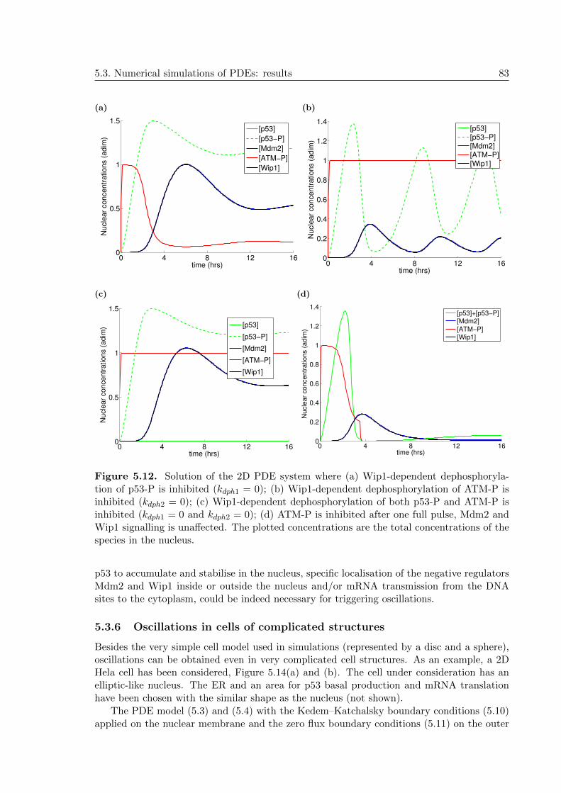
5.3. Numerical simulations of PDEs: results 83
(a)
0 4 8 12 160
0.5
1
1.5
time (hrs)
Nucle
ar
concentr
ations (
adim
)
[p53]
[p53−P]
[Mdm2]
[ATM−P]
[Wip1]
(b)
0 4 8 12 160
0.2
0.4
0.6
0.8
1
1.2
1.4
time (hrs)
Nucle
ar
concentr
ations (
adim
)
[p53]
[p53−P]
[Mdm2]
[ATM−P]
[Wip1]
(c)
0 4 8 12 160
0.5
1
1.5
time (hrs)
Nucle
ar
concentr
ations (
adim
)
[p53]
[p53−P]
[Mdm2]
[ATM−P]
[Wip1]
(d)
0 4 8 12 160
0.2
0.4
0.6
0.8
1
1.2
1.4
time (hrs)
Nucle
ar
concentr
ations (
adim
)
[p53]+[p53−P]
[Mdm2]
[ATM−P]
[Wip1]
Figure 5.12. Solution of the 2D PDE system where (a) Wip1-dependent dephosphoryla-tion of p53-P is inhibited (kdph1 = 0); (b) Wip1-dependent dephosphorylation of ATM-P isinhibited (kdph2 = 0); (c) Wip1-dependent dephosphorylation of both p53-P and ATM-P isinhibited (kdph1 = 0 and kdph2 = 0); (d) ATM-P is inhibited after one full pulse, Mdm2 andWip1 signalling is unaffected. The plotted concentrations are the total concentrations of thespecies in the nucleus.
p53 to accumulate and stabilise in the nucleus, specific localisation of the negative regulatorsMdm2 and Wip1 inside or outside the nucleus and/or mRNA transmission from the DNAsites to the cytoplasm, could be indeed necessary for triggering oscillations.
5.3.6 Oscillations in cells of complicated structures
Besides the very simple cell model used in simulations (represented by a disc and a sphere),oscillations can be obtained even in very complicated cell structures. As an example, a 2DHela cell has been considered, Figure 5.14(a) and (b). The cell under consideration has anelliptic-like nucleus. The ER and an area for p53 basal production and mRNA translationhave been chosen with the similar shape as the nucleus (not shown).
The PDE model (5.3) and (5.4) with the Kedem–Katchalsky boundary conditions (5.10)applied on the nuclear membrane and the zero flux boundary conditions (5.11) on the outer

84 5. Reaction-diffusion model for the p53 network
0 4 8 12 160
1
2
3
4
5
6
time (hrs)
Co
nce
ntr
atio
ns (
ad
im)
[p53]+[p53−P]
[Mdm2]
[ATM−P]
[Wip1]
Figure 5.13. Solution of the 2D PDE system following DNA damage producing the tran-siting signal E = 1 in the case when both compartments are merged together. The plottedconcentrations are the total concentrations in the nucleus.
cellular membrane is then solved on the triangulation generated by FreeFem++. The kineticrates, diffusion and translocation parameters remain the same as in Tables 5.5 and 5.2 (exceptfor the p53 basal production rate which is set to 0.03µM/min). The semi-implicit Rothemethod then gives oscillations in the p53 dynamics following exposition to a stress signal ofthe amount of E = 1, see Figures 5.15(a) and (b) where the nuclear and cytoplasmic (dimen-sionless) concentrations of the proteins are plotted, Fig. 5.15(c) for a particular phase planethat confirm existence of (stable) limit cycles in the protein evolutions, and also Figures 5.16and 5.17 where six different samples from the concentrations of p53 and Mdm2 are captured:at the initial time 0 and the times when either p53 or Mdm2 reach its maximum. In thesimulation the obtained solutions show oscillations of the period ∼6.3 hours.
5.4 Discussion and conclusions from the PDE model #1
Based on the recently observed oscillations of the p53 protein in single cells [15, 56, 77],we have proposed a spatio-temporal RD model counting the negative feedback p53-Mdm2together with ATM-p53-Wip1 and compartmental distinction of cellular events between thenucleus and the cytoplasm.
We have shown that spatial variables and the PDE model can be used to simulate thebehaviour of the p53 intracellular network in the stressed cells as well as by ODE models.The oscillations obtained from PDEs are driven by a spatial representation, diffusivities andpermeabilities of the species, since in the PDE model they have to overcome distances diffu-sively to reach targets and particular areas in the cell, e.g. to reach the translations sites formRNAs to be translated into proteins, which is not the case of ODEs. Translocation throughthe nuclear membrane, which is modelled by the Kedem–Katchalsky BC, is also affectedby diffusivity of the species. For example, Mdm2, which acts only in the nucleus, diffusivelyspreads over the entire cytoplasm after leaving the translation sites, which decreases its abun-dance at the nuclear membrane and so the level of the protein at the membrane that can bepotentially translocated into the nucleus. Notably, a single mRNA export from the nucleus tothe cytoplasm may take 10–30 minutes [16]. Thus, diffusive motion and membrane translo-cation impose a delay in the protein/mRNA translocation between the compartments which,afterwards, affects the dynamics (amplitudes and periods) of their concentration. Transloca-

5.4. Discussion and conclusions from the PDE model #1 85
(a) (b)
Figure 5.14. (a) Healthy HeLa cells surrounding apoptotic HeLa cell (center). Visible partsare the nucleus (blue), fibres (red) and Golgi’s apparatus (yellow). (b) One particular cellchosen for simulations (nucleus is in green, cytoplasm in blue). Image courtesy of ThomasDeerinck and Mark Ellisman (NCMIR and UCSD) [33].
tion in ODEs is simplified in the way that the actual concentrations at the nuclear membraneare the concentrations in the whole compartments thus independent of the effect of diffusivemovement. Hence, diffusivity, the time the species need to reach membranes, compartmentsand the translation zones within the cytoplasm, translocation through the nuclear membrane(controlled by the permeability of the membrane), etc., regulate p53 dynamics by imposingsufficient physiological delays, resulting in sustained oscillations.
The diffusion rates chosen here (∼1000µm2/min for p53, Mdm2 and Wip1) lie at theupper bound of the estimated range of acceptable diffusion coefficients for p53 and Mdm2 forwhich simulations in [43] yield oscillations. The estimated range of the diffusion parameters,for which our PDE system gives oscillations, is rather wide (even with no upper bounds in 2Dand 3D simulations, Table 5.3) compared with the range 10− 1000µm2/min for the proteindiffusivity obtained in [43] and the range 4.44 − 150µm2/min given by the PDE model in[142] for the diffusivities of both proteins and mRNAs.
Sustained oscillations can be reproduced in cells with complicated morphologies as inthose in Figure 5.14, however, with some restrictions on the permeability of the nuclearmembrane. These restrictions can be partially abolished by the inclusion of the well definedER, although the ER does not necessarily have to present smooth boundaries. Hence, theER around the nucleus may set limits on the range of acceptable permeabilities needed foroscillations; the narrower the ER is, the smaller range of permeabilities for oscillations couldbe used.
Unlike with the chosen set of parameters in the ODE model shown in Table 3.1, in thePDE model presented here we have slightly changed some rates, in particular, unknownparameters in the expression of Wip1 by p53 so that Wip1 and Mdm2 transcription by p53runs with no affinity of p53 for these target genes. The are also some other differences betweenthe ODE and PDE models. In particular, unlike the ODE model, the PDE model containsalso two variables for the ATM monomer and ATM dimer (with different reaction terms),equations of which were not merged to one using the conservation of the total amount ofATM. In addition, we do not consider equations for the“free” but rather for the total Wip1and Mdm2 mRNA, Mdm2 is assumed to be strictly nuclear and transcription of Mdm2 andWip1 genes is mediated by phosphorylated and unphosphorylated p53.
Bearing in mind the expected behaviour of p53, i.e. turning off its oscillations at some

86 5. Reaction-diffusion model for the p53 network
(a)
0 6 12 18 240
0.5
1
1.5
2
2.5
3
3.5
time (hrs)
Nucle
ar
concentr
ations (
adim
)
[p53]+[p53−P]
[Mdm2]
[ATM−P]
[Wip1]
(b)
0 6 12 18 240
0.05
0.1
0.15
0.2
0.25
0.3
0.35
0.4
time (hrs)
Cyto
pla
sm
ic c
oncentr
ations (
adim
)
[p53][Mdm2][Wip1]
(c)
0 1 2 3 40
0.1
0.2
0.3
0.4
0.5
Nuclear [p53]+[p53−P]
Nucle
ar
[Mdm
2]
Figure 5.15. Solution of the 2D system on the HeLa cell: nondimensionalised (a) nuclearand (b) cytoplasmic concentrations of p53 (p53 and p53-P), Mdm2, ATM-P and Wip1 pro-teins. The plotted concentrations are the total concentrations in the nucleus and cytoplasm,respectively; (c) phase portrait of the nuclear concentration of p53 (p53 and p53-P) withrespect to the nuclear concentration of Mdm2.
point and establishing a steady state of high levels signalising started apoptosis, the parameterset, just mentioned differences between the models, and the chosen reference concentrationsfor the proteins used in nondimensionalisation in the ODE system turned the system to exhibittwo Hopf bifurcation points signalising two qualitatively different states for the damage signalE, the main bifurcation parameter under consideration (see Section 2.2.1 for the introductionof E). Indeed, a bifurcation analysis of the ODE system in Chapter 3 with respect to E revealstwo supercritical Hopf bifurcation points in the equilibrium curve starting at E = 0. Theequilibrium changed from stable to unstable by passing through the first Hopf point E1 andthen back from being unstable to stable when E crosses the second Hopf point E2. Thismeans that the solution bifurcates between two qualitatively different states: convergenceto a steady state for E < E1 and E > E2, and convergence to a stable limit cycle forE1 < E < E2.
We speculate that these Hopf points E1 and E2 may represent in a very summarised formkey points in the p53-mediated cell fate decisions. In particular, whenever p53 oscillatorysignalling is necessary for DNA repair, the damaged DNA signal E is produced so that

5.4. Discussion and conclusions from the PDE model #1 87
(a) 0 h (b) 2.8 h (c) 4.4 h
(d) 9.6 h (e) 11.4 h (f) 16 h
Figure 5.16. 2D visualisation of the solution of the PDE system for the HeLa cell: nondi-mensionalised concentration of p53-P and p53. The chosen samples are captured at 6 timepoints when p53 and Mdm2 reach peaks in the concentration.
E1 < E < E2. For these values of E, p53 sustainedly oscillates with a possible physiologicalinterpretation of the oscillations as a periodical examination of persistence of DNA DSB asproposed in [15, 77]. If the number of DSB decreases in repair processes and p53 oscillationsare not needed anymore, then also E might decrease, and become potentially smaller thanE1 or completely extinct if the DNA damage is successfully fixed. Therefore, E might turnoff the oscillations of the proteins. This speculation can be partially supported by someexperiments, for example, it has been reported in [13] that transient and temporal DNADSB (as the occasional ones occurring in DNA synthesis) do not result in ATM and p53oscillations, and these occasional DSB may be related to E < E1. However, if DSB persist,even more when their number increases, and/or it is impossible to repair them, then the cellmight decide to launch apoptosis with amplified E so that E trespasses the threshold E2.In apoptotic cells then the concentration of p53 leaves oscillations and approaches its steadystate of high values, for example, due to the compartmental regulation of the proteins in the

88 5. Reaction-diffusion model for the p53 network
(a) 0 h (b) 2.8 h (c) 4.4 h
(d) 9.6 h (e) 11.4 h (f) 16 h
Figure 5.17. 2D visualisation of the solution of the PDE system for the HeLa cell: nondi-mensionalised concentration of Mdm2. The chosen samples are captured at 6 time pointswhen p53 and Mdm2 reach peaks in the concentration.
p53 pathway, as an Akt-dependent inhibition of Mdm2 translocation into the nucleus in suchcells [24, 58].
The activation signal E is understood as the measure of the DNA damage, and we assumethat it is positively correlated with the damage doses (the higher doses a cell is exposed to, thebigger number of DSB is caused, the stronger activation signal E is produced; although closeridentification of E with the number of DSB is not resolved in our works). Experiments on thep53 signalling network in single cells show that the oscillations can be observed independentlyof the damage dose and that the probability for starting pulsatile response becomes greaterwith the increasing number of DSB [56, 91]. Thus, based on such strong evidence, theoscillations of the system should not become extinct with increasing E as it was modelledby the ODE model provided that E corresponds to the damage dose. The signal E in theODE model apparently plays a stronger role in the p53 signalling since “it can turn off theoscillations by itself”. However, further studies need to be done to somehow give a biological

5.4. Discussion and conclusions from the PDE model #1 89
basis to our abstract parameter E and either accept or reject our speculations.The PDE system presented in this chapter and the ODE model in the previous exhibit
a supercritical Hopf point starting from which, when E increases, the solution maintainssustained oscillations instead of converging to a steady state. This bifurcation point can havea biological explanation as above. However, the second point for which sustained oscillationsare switched back into the convergence to a steady state by crossing this point does notappear anymore in the present study as illustrated in Figures 5.11. Thus, as it has beenreported in [56, 77], p53 oscillations can be modelled as a response of the cell to stress agentsindependently of the abundance of such agents, i.e. the oscillations are not turned off just byconsidering increased DNA damage.
Apoptosis of the cell can still be accompanied by the concentration of p53 switched fromthe oscillatory response to the DNA damage to a stable steady state of high levels. Notethat the p53 sustained oscillations observed in [15, 56, 77], which can persist as long as 3days (and possibly longer), have been demonstrated in breast cancer cells MCF-7 lackingfunctional PTEN protein, thus, indeed, the p53-PTEN-PIP3-Akt positive feedback may playan essential role in cell fate decisions [24, 58]. The compartmental ODE models [126, 161]consider effects of this particular positive feedback. It is, for example, proposed in [126] thatthe p53-PTEN-PIP3-Akt positive feedback works as a clock behind the p53-Mdm2 negativefeedback, which gives some time (∼15 hours) to repairing processes to fix the DNA damage,otherwise, irreversible apoptosis is launched. In addition, the p53-Mdm2 negative feedbackalone is used to gain sustained oscillations in [126], however, it has been shown inefficientto produce oscillations in vivo [15]. The ODE model in [161] consists of the two negativefeedbacks as they are considered in our models. A cell fate decision is determined by one of thetwo different p53 states, p53-arrester and p53-killer, the latter overcoming the former. Thep53-arrester firstly transcribes proarrest genes (Wip1 and p21) and subsequently blocks thecell cycle, while p53-killer transcribes proapoptotic genes (PTEN , p53DINP1 and p53AIP1)later on, thus directing the cell to death. Note that this concept is based on the affinity ofp53 for the target genes that contradicts recently published observations in [73, 102].
At this step of modelling we have represented and simulated p53 immediate responsesto various stress conditions disrupting the integrity of the genome, such as γ-radiation ordrugs in chemotherapies causing DNA DSB. In such cases, the DNA damage sensor ATMactivates p53, thus endowing it with the ability to subsequently act as a transcription factor.Such responses to stress agents can be very sensitive in mammalian cells and our models alsoshow sensitivity in producing oscillatory responses for very low values of the damage signal,E. On the other side, the duration of the oscillatory response is not terminated purely byincreasing E.
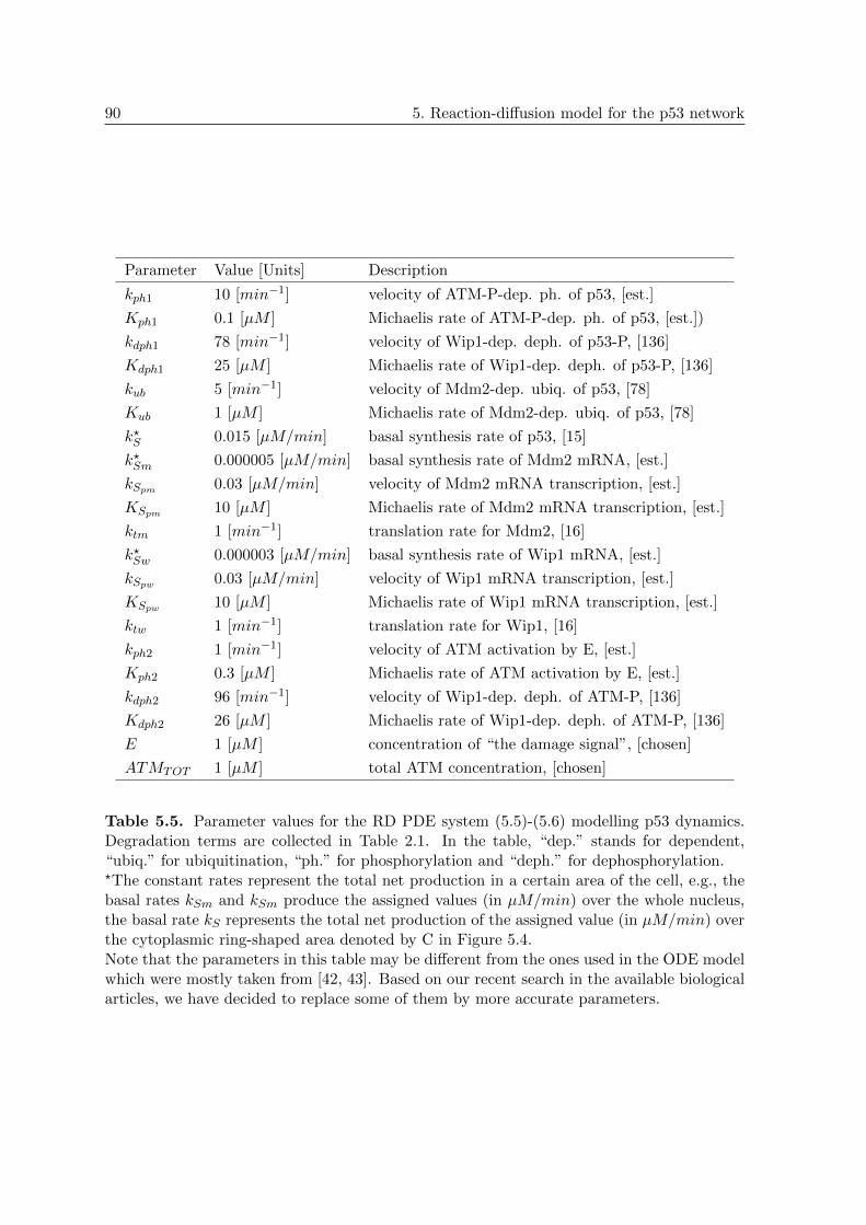
90 5. Reaction-diffusion model for the p53 network
Parameter Value [Units] Description
kph1 10 [min−1] velocity of ATM-P-dep. ph. of p53, [est.]
Kph1 0.1 [µM ] Michaelis rate of ATM-P-dep. ph. of p53, [est.])
kdph1 78 [min−1] velocity of Wip1-dep. deph. of p53-P, [136]
Kdph1 25 [µM ] Michaelis rate of Wip1-dep. deph. of p53-P, [136]
kub 5 [min−1] velocity of Mdm2-dep. ubiq. of p53, [78]
Kub 1 [µM ] Michaelis rate of Mdm2-dep. ubiq. of p53, [78]
k?S 0.015 [µM/min] basal synthesis rate of p53, [15]
k?Sm 0.000005 [µM/min] basal synthesis rate of Mdm2 mRNA, [est.]
kSpm 0.03 [µM/min] velocity of Mdm2 mRNA transcription, [est.]
KSpm 10 [µM ] Michaelis rate of Mdm2 mRNA transcription, [est.]
ktm 1 [min−1] translation rate for Mdm2, [16]
k?Sw 0.000003 [µM/min] basal synthesis rate of Wip1 mRNA, [est.]
kSpw 0.03 [µM/min] velocity of Wip1 mRNA transcription, [est.]
KSpw 10 [µM ] Michaelis rate of Wip1 mRNA transcription, [est.]
ktw 1 [min−1] translation rate for Wip1, [16]
kph2 1 [min−1] velocity of ATM activation by E, [est.]
Kph2 0.3 [µM ] Michaelis rate of ATM activation by E, [est.]
kdph2 96 [min−1] velocity of Wip1-dep. deph. of ATM-P, [136]
Kdph2 26 [µM ] Michaelis rate of Wip1-dep. deph. of ATM-P, [136]
E 1 [µM ] concentration of “the damage signal”, [chosen]
ATMTOT 1 [µM ] total ATM concentration, [chosen]
Table 5.5. Parameter values for the RD PDE system (5.5)-(5.6) modelling p53 dynamics.Degradation terms are collected in Table 2.1. In the table, “dep.” stands for dependent,“ubiq.” for ubiquitination, “ph.” for phosphorylation and “deph.” for dephosphorylation.?The constant rates represent the total net production in a certain area of the cell, e.g., thebasal rates kSm and kSm produce the assigned values (in µM/min) over the whole nucleus,the basal rate kS represents the total net production of the assigned value (in µM/min) overthe cytoplasmic ring-shaped area denoted by C in Figure 5.4.Note that the parameters in this table may be different from the ones used in the ODE modelwhich were mostly taken from [42, 43]. Based on our recent search in the available biologicalarticles, we have decided to replace some of them by more accurate parameters.

6
Novel mechanism for p53oscillations: positive role of thenegative regulator Mdm2
It is generally accepted that Mdm2 is a dominant negative regulator of p53 estab-lishing its homeostasis in DNA damage response [147]. As it is mentioned in theprevious sections, there exist several negative feedback loops regulating p53, most ofthem between p53 and Mdm2 [60]. However and somehow surprisingly, in additionto targeting p53 for degradation, Mdm2 in tight cooperation with MdmX can controlexpression levels of p53 through the enhanced induction of p53 synthesis in responseto DNA damage [54, 96]. Whilst ATM-dependent phosphorylation of p53 is not ob-served to be important in this enhanced synthesis, ATM-dependent phosphorylationof Mdm2 (as well as MdmX) is essential for its dual role which is accompanied withwidely oscillating p53. In the light of these new observations we formulate a novelmechanism for p53-Mdm2 dynamics and show that this mechanism is sufficient totrigger p53 oscillations. Notably, p53 excitable response to a transient input [15]can be explained by this dual function of Mdm2.
Organisation of the chapter is as follows: Section 6.1 introduces new biological ob-servations and a dual function of Mmd2 to p53. A model of p53 dynamics takinginto account positive and negative role of Mdm2 towards p53 is developed and exam-ined in Section 6.2. Section 6.3 is then devoted to a phenomena of p53 excitabilitywhich is shown to occur in response to DSB caused by γ-irradiation or drugs.
6.1 Mdm2’s dual function toward p53 in DDR
Recent observations suggest that Mdm2 can regulate p53 synthesis. In particular, Mdm2 caninduce translation of p53 mRNA from two alternative initiation sites, giving a full-length p53and an isoform of p53 with a relative molecular mass of approximately 47 kDa. This isoformdoes not contain the Mdm2-binding site and it lacks the amino-terminal transcriptional-activation domain of p53, however, its abundance positively regulates stabilisation of thefull-length p53 in the presence of Mdm2. In addition, the p53 translation induction can beaffected by Mdm2 and this regulation of p53 synthesis requires Mdm2 to interact directlywith the nascent p53 mRNA [158].
In the more recent studies [54, 96], R. Fahraeus and his colleagues discovered and de-scribed the precise molecular mechanism of a positive role of Mdm2 and its homolog MdmX
91
92 6. Novel mechanism for p53 oscillations: positive role of the negative regulator Mdm2
in the regulation of p53. In particular, they observed that Mdm2 as well as MdmX1 canbind and form complexes with p53 mRNA following phosphorylation of Mdm2 at Ser395 [54]and MdmX at Ser403 [96] both by ATM. ATM-dependent phosphorylation of Mdm2 was notfollowed by Mdm2-P rapid degradation in [54] as it was observed in [139], but this phospho-rylation event led to its nucleoli accumulation where Mdm2 changed its function from beinga negative to a positive regulator of p53 [54]. In the first instance, the phosphorylated MdmXbinds the nascent p53 mRNA and promotes its conformational changes in a way that favoursattraction of the phosphorylated Mdm2 to the complex [96].
Action of MdmX-P on p53 mRNA following DNA damage relies on specific folding ofthe mRNA and MdmX-P can bind to a newly born mRNA at the DNA site only. In thep53 mRNA-MdmX-Mdm2 complexes MdmX acts as the “RNA chaperone” during its trans-portation from the nucleus to the cytoplasm [96]. Further, Mdm2 bound to the complexis much less capable to ubiquitinate p53 for degradation and, on the other hand, it stimu-lates p53 mRNA translation after genotoxic stress [54, 96]. In fact Mdm2-P induces morethan three-fold increase in the rate of p53 synthesis after cells were exposed to doxorubicin[54, 96]. In addition, the wild-type p53 protein expressed from a non-Mdm2 binding mRNAis hyperunstable in the presence of Mdm2 in DDR. Thus the significance of the p53 mRNA-MdmX-Mdm2 complexes is not only in increasing p53 levels (through the enhanced p53synthesis) but also in preventing p53 degradation following genotoxic stress (through thesuppressed p53 ubiquitination) [54].
ATM-dependent phosphorylation of Mdm2 and MdmX is required for p53 mRNA-MdmX-Mdm2 interactions. Indeed, while phosphorylation of Mdm2 by ATM promoted its interactionwith p53 mRNA, nonphosphorylated Mdm2 had weak affinity for p53 mRNA [54]. Phospho-rylation of either of the two proteins supports formation of Mdm2-MdmX oligomers; non-phosphorylated Mdm2 interacts with MdmX and prevents its RNA chaperone activity [96].In addition, Mdm2’s Ser3952 phosphorylation site is sufficient and necessary for the stabilityof p53 mRNA-Mdm2 complexes with a 3-5 fold increased abundance of p53 mRNA [54].ATM-mediated phosphorylation of MdmX at Ser403 induces a highly specific binding to thep53 which is similar to that of Mdm2, however, MdmX does not stimulate its translation [96].
As described in Section 1.2.2, the generally accepted model for stabilisation of p53 re-quires phosphorylation of p53 by ATM, which enables p53 to escape from Mdm2-mediateddegradation. Nevertheless, ATM-mediated phosphorylation of p53 was not observed to benecessary in the stabilisation of p53 and in order for Mdm2 to enhance p53 activity in re-sponse to DNA damage in [54]. In the line with this observation, close examination of allpossible phosphorylation sites of p53 revealed that the site Ser15 may not have any directeffects on binding p53 to Mdm2 (although it is still necessary for the transcriptional activa-tion of p53). Phosphorylation of p53’s Thr18 is the only event found to significantly inhibitthe ability of Mdm2 to bind p53 [131].
Thus, all these results demonstrate how ATM activity can switch between the two oppositeroles of Mdm2 in the regulation of p53: depending on its phosphorylations status Mdm2targets either p53 mRNA or p53, see Figure 6.1. This also suggests a novel mechanism whichcould possibly explain p53 oscillations after genotoxic stress. In the following section we
1It is known from previous studies that MdmX can form a complex with p53, bind to the same domainas Mdm2 (thus it competes with Mdm2 binding), yet it possesses no E3 activity and does not target p53for degradation. However, p53 which accumulates in the presence of MdmX is biochemically and biologicallyinactive [106].
2Importance of this site for the increased activity of p53 is also evident from a significant reduction inapoptosis in several cell lines following the treatment with doxorubicin, including AT5-BIVA, H1299, andDKO cells which express ATM and wt p53 (of a smaller amount compared to wt Mdm2) but with Mdm2mutated at Ser395 [54].

6.2. A novel mechanism for p53 oscillations 93
Figure 6.1. Positive effect of Mdm2 and MdmX towards p53: In the presence of DNAdamage, ATM dimers dissociate into active monomers which phosphorylate Mdm2 at Ser395and MdmX at Ser403 in the nuclear compartment. Phosphorylated Mdm2 and MdmX thenform a complex with a nascent p53 mRNA, fold it and move from the nucleus to the cytoplasm,passing likely through the nucleolus where Mdm2 switches into a positive regulator of p53 byincreasing p53 synthesis and, at the same time, suppressing Mdm2-dependent degradationof p53. This all enables p53 to accumulate in the nucleus where it acts as a transcriptionfactor for the Mdm2 and Wip1 (and other) genes. The phosphatase Wip1 targets ATM-Pfor inactivation. Wip1 reverses also Mdm2 and MdmX phosphorylation status so that Mdm2promotes ubiquitination and degradation of p53. The persistent DNA damage signal cantrigger another pulse of p53 by ATM dimer monomerisation again.
propose a model for this mechanism. It is based on a simple conclusion from the observationsabove: as long as the ATM signalling is active, Mdm2 serves as a positive regulator of p53,whilst p53 is rapidly degraded by Mdm2 when the DDR is terminated (via the action of Wip1[52, 92]).
6.2 A novel mechanism for p53 oscillations
A model for the molecular network composed of the negative feedback loops p53→Mdm2 ap53 and ATM -P → Mdm2 → p53 → Wip1 a ATM -P situated in the spatial PDE frame-work is presented in this section. The model is simplified in the sense that MdmX, whichacts in the tight cooperation with Mdm2, is omitted from further considerations3.
3Partly because MdmX and possibly its mRNA would represent another variables in the model.

94 6. Novel mechanism for p53 oscillations: positive role of the negative regulator Mdm2
Figure 6.2. A simplified positive effect of Mdm2 towards p53: ATM dimers dissociateinto active monomers ATM-P after DNA damage which then phosphorylate Mdm2 in thenuclear compartment. Phosphorylated Mdm2 switches into a positive regulator of p53, bindsto a nascent p53 mRNA at the DNA site and moves with mRNA from the nucleus to thecytoplasm. In the cytoplasm, p53 mRNA from the complex is translated with a highertranslation rate than p53 from “non-complex mRNA”. At the same time, Mdm2-dependentdegradation of p53 is decreased. p53 then translocates to the nucleus where it acts as atranscription factor for the Mdm2 and Wip1 (and other) genes. The phosphatase Wip1targets ATM-P for inactivation. Wip1 also dephosphorylates Mdm2 so that Mdm2 promotesubiquitination and degradation of p53. The persistent DNA damage signal can trigger anotherpulse by ATM dimer monomerisation again.
A novel model for p53 oscillations which we propose runs as follows, see also Figure 6.2:Following DNA damage, Mdm2 is phosphorylated by ATM and the phosphorylated Mdm2-Ptargets p53 mRNA instead of the protein p53. Mdm2-P acts as a chaperone for the mRNA,moves with it to the cytoplasm and together with p53 mRNA binds to free ribosomes. ThemRNA is then translated with an increased synthesis rate giving the p53 protein. Meanwhile,p53 accumulates in the nucleus where it acts as a TF for the Mdm2 and Wip1 genes. In turn,Wip1 dephosphorylates Mdm2-P and the dephosphorylated Mdm2 targets p53 for degrada-tion. Wip1 also dephosphorylates ATM-P trying to establish homeostasis in the DDR. Thiscloses the first cycle between the antagonists. We do not consider any DNA repair mechanismhere, thus persistent DNA damage signal E4 triggers another wave of ATM-P and consequentpulses in all the other proteins under consideration.
4See Section 2.2.1 for the introduction of the substrate E.

6.2. A novel mechanism for p53 oscillations 95
χL
χCD
ER
Figure 6.3. A scheme of the cell used in the model: the cell is represented by a disc withradius 10µm. It consists of the nucleus represented by an inner disc of radius 3µm andthe cytoplasm containing the rest of the cell. Within the cytoplasm there is an endoplasmicreticulum (ER) where no translation of the mRNAs occurs. The ER is represented by anannulus with radii 3µm and 5µm. Translation of the mRNAs is supposed to occur outsideof the ER, thus in an annulus χCD with radii 5 and 10µm. Inside the nucleus there is asmall disc χL of radius 1µm which represents the DNA locus where production of all mRNAcontent occurs.
6.2.1 Modelling Mdm2’s dual function: assumptions
In contrast to the previous p53 PDE model (equations (5.5) and (5.6), hereafter denotedby Model 1) where we did not consider p53 mRNA, the new model relies on the synthesisof the mRNA either bound or unbound to the phosphorylated Mdm2 protein. FollowingATM-dependent phosphorylation of Mdm2, Mdm2-P binds nascent p53 mRNA at the DNAsites in the nucleus thus, for simplicity, we specify a small area inside the nucleus as a “DNAlocus” (denoted by χL on Fig. 6.3) where p53 mRNA is produced with a constant rate, andwe assume that the reaction
p35 mRNA+Mdm2-Pka−→ C
with an association rate ka occurs in this area χL only5. Here C denotes the p53 mRNA-Mdm2-P complex which moves to the cytoplasm where it binds free ribosomes, and similarlyto the previous model, ribosomes are assumed to be located outside of the endoplasmicreticulum. The complex C can dissociate back into p53 mRNA and Mdm2-P in the cytoplasm,thus following the reaction
Ckd−→ p35 mRNA+Mdm2-P
with a dissociation rate kd. When it is released from C, p53 mRNA can be again used inthe translation process; however, Mdm2-P cannot bind such mRNA again nor any other p53
5The Law of Mass action is then used to rewrite this reaction into mathematical terms.

96 6. Novel mechanism for p53 oscillations: positive role of the negative regulator Mdm2
mRNA outside the DNA locus χL in the nucleus.
The half-life of the complex C is set to 1 hour in this model which is the same as thehalf-lives of Mdm2 and Wip1 mRNA and 3-fold longer than the half-life of “free” p53 mRNAnot bound to C (i.e., 20 minutes in accord with [1] who claim that the half-lives of mRNA ofshort-lived proteins such as transcription factors is often shorter than 30 minutes).
Since p53 produced from the mRNA bound to Mdm2-P is more stable (hereafter denotedby p53-2) when compared with the stability of p53 produced from the “free” mRNA (whichwas not bound to Mdm2-P; hereafter denoted by p53-1), the turnover constant for ubiqui-tination of p53-2 by both Mdm2 and Mdm2-P, i.e., kub-2 = 1min−1, is chosen to be 5-foldsmaller than the ubiquitination rate (kub-1 = 5min−1) reported in [78]. The “unstable” p53-1is targeted for ubiquitination by Mdm2 with the rate kub-1 and by Mdm2-P with the ratekub-2
6. The Michaelis constant of the ubiquitination process is the same (Kub = 1µM) forboth p53-1 and p53-2 ubiquitination. Natural and Mdm2-independent degradation rates forboth p53-1 and p53-2 correspond to the half-life of 7 hours. Natural degradation rates forMdm2 and Mdm2-P are the same (Table 2.1).
Both proteins p53-1 and p53-2 are translated with different rates, since the synthesis ofp53-2, when produced from p53 mRNA bound to the complex C, is enhanced 3–4-fold dueto the active role of Mdm2-P. Thus we will consider two translation rates: ktp-1 for p53-1which is equal to the translation rates for Mdm2 and Wip1 (as they are used in the previousModel 1) and ktp-2 for p53-2 which is 3-times larger than ktp-1. In the transcription processof the Mdm2 and Wip1 genes, both proteins p53-1 and p53-2 act in a synergistic way, i.e.,we do not distinguish between them whenever they are supposed to do the transcription job.Rates for p53-dependent synthesis of Mdm2 and Wip1 are the same as in the previous model.Transcription of the genes is supposed to occur in the DNA locus χL.
We will also assume that all proteins under consideration are nuclear proteins in the sensethat they move from the translation sites in the cytoplasm (outside the ER) to the nucleus.On the other side, mRNAs and the complex C move from the nucleus to the cytoplasm. Allthese translocations are unidirectional.
We do not consider p53 phosphorylation by ATM in this model, and as in the previousmodel we include both equations for the nuclear monomeric and dimeric ATM protein. Whilethe parameters (kph3 and Kph3) for ATM-dependent phosphorylation of Mdm2 are not known(and thus were tuned by hand), the rates kdph3 and Kdph3 for newly added Wip1-dependentdephosphorylation of Mdm2-P are taken from [155]. Other relevant parameters are the sameas in the previous PDE model and all kinetic rates are listed in Table 6.2, natural degradationrates in Table 2.1. As far as we are concerned with the diffusion and permeability rates forthe complex C and p53 mRNA unbound to C, we assume that they are equal to the diffusionand permeability rate of an average mRNP compound (i.e., DC = DpRNA = 1.8µm2/minand pC = ppRNA = 0.1µm/min, pRNA stands for p53 RNA); diffusions and permeabilitiesare also the same for the pairs p53-1 and p53-2, and Mdm2 and Mdm2-P, respectively. Allthe relevant diffusion and permeability rates are listed in Table 5.2.
Protein-protein interactions are modelled as the enzyme reactions and thus, using theLMA and QSSA, the specific terms in the equations are composed from Michaelis functions.Transcription of the Mdm2 and Wip1 genes is modelled by Hill functions with the coefficient4. Thus new equations, as shown in the following section, resemble equations (5.5) and (5.6)from the previous PDE model.
6Thus, we assume a certain level of a lowered affinity of Mdm2-P for p53 (both p53-1 and p53-2). In otherwords, ATM-dependent phosphorylation of Mdm2 reduces the ability of Mdm2-P to ubiquitinate both p53-2(more stable) and p53-1 (less stable). Increased stability of p53-2 is achieved through a decreased ability ofnon-phosphorylated Mdm2 to ubiquitinate p53-2.
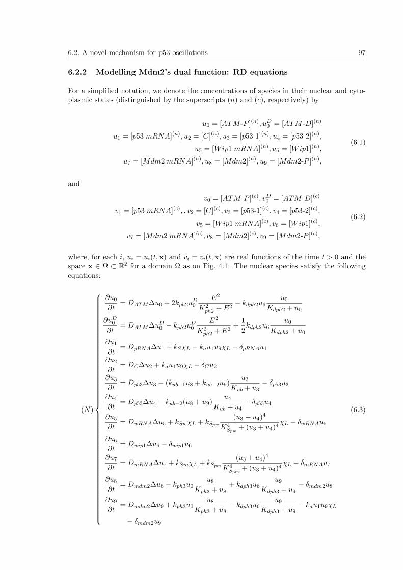
6.2. A novel mechanism for p53 oscillations 97
6.2.2 Modelling Mdm2’s dual function: RD equations
For a simplified notation, we denote the concentrations of species in their nuclear and cyto-plasmic states (distinguished by the superscripts (n) and (c), respectively) by
u0 = [ATM -P ](n), uD0 = [ATM -D](n)
u1 = [p53 mRNA](n), u2 = [C](n), u3 = [p53-1](n), u4 = [p53-2](n),
u5 = [Wip1 mRNA](n), u6 = [Wip1](n),
u7 = [Mdm2 mRNA](n), u8 = [Mdm2](n), u9 = [Mdm2-P ](n),
(6.1)
and
v0 = [ATM -P ](c), vD0 = [ATM -D](c)
v1 = [p53 mRNA](c), , v2 = [C](c), v3 = [p53-1](c), v4 = [p53-2](c),
v5 = [Wip1 mRNA](c), v6 = [Wip1](c),
v7 = [Mdm2 mRNA](c), v8 = [Mdm2](c), v9 = [Mdm2-P ](c),
(6.2)
where, for each i, ui = ui(t,x) and vi = vi(t,x) are real functions of the time t > 0 and thespace x ∈ Ω ⊂ R2 for a domain Ω as on Fig. 4.1. The nuclear species satisfy the followingequations:
(N)
∂u0
∂t= DATM∆u0 + 2kph2u
D0
E2
K2ph2 + E2
− kdph2u6u0
Kdph2 + u0
∂uD0∂t
= DATM∆uD0 − kph2uD0
E2
K2ph2 + E2
+1
2kdph2u6
u0
Kdph2 + u0
∂u1
∂t= DpRNA∆u1 + kSχL − kau1u9χL − δpRNAu1
∂u2
∂t= DC∆u2 + kau1u9χL − δCu2
∂u3
∂t= Dp53∆u3 − (kub−1u8 + kub−2u9)
u3
Kub + u3− δp53u3
∂u4
∂t= Dp53∆u4 − kub−2(u8 + u9)
u4
Kub + u4− δp53u4
∂u5
∂t= DwRNA∆u5 + kSwχL + kSpw
(u3 + u4)4
K4Spw
+ (u3 + u4)4χL − δwRNAu5
∂u6
∂t= Dwip1∆u6 − δwip1u6
∂u7
∂t= DmRNA∆u7 + kSmχL + kSpm
(u3 + u4)4
K4Spm
+ (u3 + u4)4χL − δmRNAu7
∂u8
∂t= Dmdm2∆u8 − kph3u0
u8
Kph3 + u8+ kdph3u6
u9
Kdph3 + u9− δmdm2u8
∂u9
∂t= Dmdm2∆u9 + kph3u0
u8
Kph3 + u8− kdph3u6
u9
Kdph3 + u9− kau1u9χL
− δmdm2u9
(6.3)
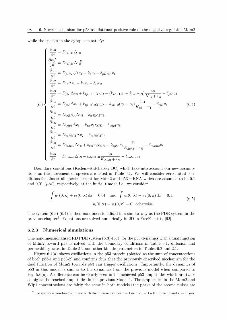
98 6. Novel mechanism for p53 oscillations: positive role of the negative regulator Mdm2
while the species in the cytoplasm satisfy:
(C)
∂v0
∂t= DATM∆v0
∂vD0∂t
= DATM∆vD0
∂v1
∂t= DpRNA∆v1 + kdv2 − δpRNAv1
∂v2
∂t= DC∆v2 − kdv2 − δCv2
∂v3
∂t= Dp53∆v3 + ktp−1v1χCD − (kub−1v8 + kub−2v9)
v3
Kub + v3− δp53v3
∂v4
∂t= Dp53∆v4 + ktp−2v2χCD − kub−2(v8 + v9)
v4
Kub + v4− δp53v4
∂v5
∂t= DwRNA∆v5 − δwRNAv5
∂v6
∂t= Dwip1∆v6 + ktwv5χCD − δwip1v6
∂v7
∂t= DmRNA∆v7 − δmRNAv7
∂v8
∂t= Dmdm2∆v8 + ktmv7χCD + kdph3v6
v9
Kdph3 + v9− δmdm2v8
∂v9
∂t= Dmdm2∆v9 − kdph3v6
v9
Kdph3 + v9− δmdm2v9
(6.4)
Boundary conditions (Kedem–Katchalsky BC) which take into account our new assump-tions on the movement of species are listed in Table 6.1. We will consider zero initial con-ditions for almost all species except for Mdm2 and p53 mRNA which are assumed to be 0.1and 0.01 (µM), respectively, at the initial time 0, i.e., we consider
ˆu1(0,x) + v1(0,x) dx = 0.01 and
ˆu8(0,x) + v8(0,x) dx = 0.1.
ui(0,x) = vi(0,x) = 0, otherwise.
(6.5)
The system (6.3)-(6.4) is then nondimensionalised in a similar way as the PDE system in theprevious chapter7. Equations are solved numerically in 2D in FreeFem++, [62].
6.2.3 Numerical simulations
The nondimensionalised RD PDE system (6.3)-(6.4) for the p53 dynamics with a dual functionof Mdm2 toward p53 is solved with the boundary conditions in Table 6.1, diffusion andpermeability rates in Table 5.2 and other kinetic parameters in Tables 6.2 and 2.1.
Figure 6.4(a) shows oscillations in the p53 protein (plotted as the sum of concentrationsof both p53-1 and p53-2) and confirms thus that the previously described mechanism for thedual function of Mdm2 towards p53 can trigger oscillations. Importantly, the dynamics ofp53 in this model is similar to the dynamics from the previous model when compared toFig. 5.6(a). A difference can be clearly seen in the achieved p53 amplitudes which are twiceas big as the reached amplitudes in the previous Model 1. The amplitudes in the Mdm2 andWip1 concentrations are fairly the same in both models (the peaks of the second pulses are
7The system is nondimensionlised with the reference values τ = 1min, αi = 1µM for each i and L = 10µm.

6.2. A novel mechanism for p53 oscillations 99
Chemical nuclear changes cytoplasmic changes
ATM-P −DATM∂u0
∂n1= 0 DATM
∂v0
∂n1= 0
ATM-D −DATM∂uD0∂n1
= 0 DATM∂vD0∂n1
= 0
p53 mRNA −DpRNA∂u1
∂n1= ppRNAu1 DpRNA
∂v1
∂n1= −ppRNAu1
C −DC∂u2
∂n1= pCu2 DC
∂v2
∂n1= −pCu2
p53-1 −Dp53∂u3
∂n1= −pp53v3 Dp53
∂v3
∂n1= pp53v3
p53-2 −Dp53∂u4
∂n1= −pp53v4 Dp53
∂v4
∂n1= pp53v4
Wip1 mRNA −DwRNA∂u5
∂n1= pwRNAu5 DwRNA
∂v5
∂n1= −pwRNAu5
Wip1 −Dwip1∂u6
∂n1= −pwip1v6 Dwip1
∂v6
∂n1= pwip1v6
Mdm2 mRNA −DmRNA∂u7
∂n1= pmRNAu7 DmRNA
∂v7
∂n1= −pmRNAu7
Mdm2 −Dmdm2∂u8
∂n1= −pmdm2v8 Dmdm2
∂v8
∂n1= pmdm2v8
Mdm2-P −Dmdm2∂u9
∂n1= −pmdm2v9 Dmdm2
∂v9
∂n1= pmdm2v9
Table 6.1. The Kedem–Katchalsky transmission boundary conditions on Γ1 with the diffu-sion coefficients Di and the translocation rates pi for the RD PDE system (6.3)-(6.4) mod-elling p53 dynamics with a dual function of Mdm2 towards p53. Whilst neither ATM dimers(ATM-D) nor ATM-P are allowed to leave nucleus, the complex C, p53, Wip1 and Mdm2mRNAs move from the nucleus to the cytoplasm and the proteins p53-1, p53-2, Mdm2 andWip1 from the cytoplasm to the nucleus as well as Mdm2-P unless it is bound to C.
equal to 0.14 in both models). One may think that the p53-dependent transcription is thendifferent in both models, and it really is in the sense that the transcription sites are reducedto the DNA locus in this model whereas the transcription was allowed in the whole nucleusin Model 1. Otherwise the parameters for the transcription of genes used in this model arethe same as in Model 1. The level of p53 (p53-1 and p53-2) appearing in the DNA locus isshown by the green dashed line in Fig. 6.4(a).
Timing of the pulses is also similar to each other in both models. The first two peaksin the p53 concentration are reached at 2.4 and 8.6hrs after damage and the period of p53oscillations in this specific example is 5.7 hours. Figure 6.5(b) further shows that the half-lifeof p53 in the cell in the presence of wt Mdm2 is 15 and 20 minutes when estimated fromthe first and second pulse, respectively. Obtained oscillations are confirmed by a limit cycleplotted on Fig. 6.5(a).
We started this simulation with a non-zero initial condition for Mdm2 and as it can beseen from Fig. 6.4(a), the Mdm2 level decreases in the first two hours. This was not causedby its degradation due to autoubiquitination (after the previous phosphorylation by ATM-P) clearly because our equations do not contain terms reflecting this phenomena. Instead,

100 6. Novel mechanism for p53 oscillations: positive role of the negative regulator Mdm2
(a)
0 5 10 15 200
0.5
1
1.5
2
2.5
time (hrs)
Nu
cle
ar
co
nce
ntr
atio
ns (
ad
im)
[p53−1]+[p53−2][p53−1]+[p53−2] in χ
L
[Mdm2]+[Mdm2−P]+[C]
[ATM−P]
[Wip1]
(b)
0 5 10 15 200
0.005
0.01
0.015
0.02
0.025
0.03
time (hrs)
Nucle
ar
concentr
ations (
adim
)
[p53 mRNA][C]
Figure 6.4. Solution of the RD PDE system (6.3)-(6.4) modelling p53 dynamics with adual function of Mdm2 toward p53. Plotted curves are the concentrations in 20hrs of DDRin response to the stress signal E = 1 for the fixed set of parameters in Tables 6.2 and 5.2:nondimensionalised (a) nuclear concentrations of total p53 (p53-1 and p53-2), total Mdm2(Mdm2, free Mdm2-P and Mdm2-P bound to C), ATM-P and Wip1; green dashed lineshows the concentration of p53 in the DNA locus χL (that is the transcriptionally activep53); (b) total cellular “free” p53 mRNA and p53 mRNA bound to the complex C. Theplotted concentrations are the total concentrations in the nucleus and cell, respectively.
Mdm2 is degraded simply because of its short half-life and new Mdm2 molecules dependtranscriptionally on p53 (its nuclear accumulation and activity). More than 2 hours afterdamage, the level of Mdm2 starts to increase and peaks at the 4hrs time point after damage,at the point when p53 is found at its minimum.
Figure 6.4(b) shows the total intracellular concentration of p53 mRNA either bound tothe complex C or “free” mRNA (unbound to C). In this case, the mRNA level in the complexC is 2.5-fold of the level of free mRNA.
In this specific case the enhanced translation from p53 mRNA bound to the complexC is necessary for oscillations. If we either do not allow the p53 mRNA-Mdm2-P complexformation (the association constant ka is set to zero) or ka > 0 remains as reported in Table 6.2but the translation rates for both p53-1 and p53-2 are the same (i.e., ktp-2 = ktp-1 = 1min−1),then we loose sustained oscillations. Instead, in the first case we observe convergence to asteady-state Figure 6.6, the p53 pattern which resembles p53 response to UV irradiation asdepicted on Fig. 6.9. In the second case (when ktp-2 = ktp-1), we obtain damped oscillationsin the p53 concentration, Figure 6.7. Sustained oscillations can be retrieved for the valueof ktp-2 ≥ 1.4min−1 and they are observed for the values of ktp-2 as big as 500min−1 (inthe latter case, the difference between the maxima in the p53 and Mdm2 nuclear levels is ofseveral orders of magnitude, which confirms that a low concentration of Mdm2 can sufficientlyremove over-expressed p53 from the nucleus).
Decreased ability of Mdm2 to target p53-2 for degradation, that is the p53 protein syn-thesised from the mRNA bound to the complex C, is essential for oscillations. The admissiblerates kub-2 of the Mdm2-dependent ubiquitination of p53-2 yielding sustained oscillations arein the range 0.02 − 3.5 min−1 which is less that the reported turnover rate kub-1 = 5min−1
in [78]. The rate kub-1 is used in the ubiquitination of p53-1.
Finally, Figure 6.8 shows dependence of the p53 concentration on varying stress signal E
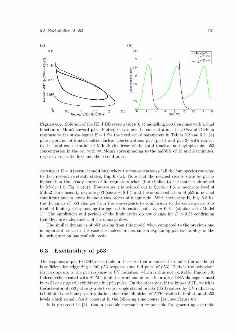
6.3. Excitability of p53 101
(a)
0 0.5 1 1.5 2 2.50
0.05
0.1
0.15
0.2
Nuclear [p53−1]+[p53−2]
Nucle
ar
[Mdm
2]+
[Mdm
2−
P]+
[C]
(b)
0 2 4 6 8 10 12 14 160
0.5
1
1.5
2
2.5
3
3.5
time (hrs)
Co
nce
ntr
atio
ns (
ad
im)
Total [p53]t1/2
= 15 min
t1/2
= 20 min
Figure 6.5. Solution of the RD PDE system (6.3)-(6.4) modelling p53 dynamics with a dualfunction of Mdm2 toward p53. Plotted curves are the concentrations in 20hrs of DDR inresponse to the stress signal E = 1 for the fixed set of parameters in Tables 6.2 and 5.2: (a)phase portrait of dimensionless nuclear concentrations p53 (p53-1 and p53-2) with respectto the total concentration of Mdm2; (b) decay of the total (nuclear and cytoplasmic) p53concentration in the cell with wt Mdm2 corresponding to the half-life of 15 and 20 minutes,respectively, in the first and the second pulse.
starting at E = 0 (normal conditions) where the concentrations of all the four species convergeto their respective steady states, Fig. 6.8(a). Note that the reached steady state by p53 ishigher than the steady states of its regulators when (but similar to the states maintainedby Model 1 in Fig. 5.5(a)). However as it is pointed out in Section 1.5, a moderate level ofMdm2 can efficiently degrade p53 (see also [61]), and the actual reduction of p53 in normalconditions and in stress is about two orders of magnitude. With increasing E, Fig. 6.8(b),the dynamics of p53 changes from the convergence to equilibrium to the convergence to a(stable) limit cycle by passing through a bifurcation point E1 = 0.011 (similar as in Model1). The amplitudes and periods of the limit cycles do not change for E > 0.25 confirmingthat they are independent of the damage dose.
The similar dynamics of p53 arising from this model when compared to the previous oneis important, since in this case the molecular mechanism explaining p53 excitability in thefollowing section has realistic basis.
6.3 Excitability of p53
The response of p53 to DSB is excitable in the sense that a transient stimulus (for one hour)is sufficient for triggering a full p53 response (one full pulse of p53). This is the behaviourjust in opposite to the p53 response to UV radiation, which is thus not excitable, Figure 6.9.Indeed, cells treated with ATM’s inhibitor wortmannin one hour after DNA damage causedby γ-IR or drugs still exhibit one full p53 pulse. On the other side, if the kinase ATR, which isthe activator of p53 pathway able to sense single strand breaks (SSB) caused by UV radiation,is inhibited one hour post-irradiation, then the inhibition of ATR results in inhibition of p53levels which remain fairly constant in the following time course [14], see Figure 6.9.
It is proposed in [14] that a possible mechanism responsible for generating excitable

102 6. Novel mechanism for p53 oscillations: positive role of the negative regulator Mdm2
(a)
0 5 10 15 200
0.2
0.4
0.6
0.8
1
time (hrs)
Nu
cle
ar
co
nce
ntr
atio
ns (
ad
im)
[p53−1]+[p53−2][p53−1]+[p53−2] in χ
L
[Mdm2]+[Mdm2−P]+[C]
[ATM−P]
[Wip1]
(b)
0 5 10 15 200
0.005
0.01
0.015
0.02
0.025
time (hrs)
Nucle
ar
concentr
ations (
adim
)
[p53 mRNA]
[C]
Figure 6.6. Solution of the RD PDE system (6.3)-(6.4) modelling p53 dynamics with adual function of Mdm2 toward p53. Plotted curves are the concentrations in 20hrs of DDRin response to the stress signal E = 1 in the case when no complex C formation is allowed(i.e., ka = 0) for the parameters in Tables 6.2 and 5.2: nondimensionalised (a) nuclearconcentrations of total p53-1 (no p53-2 is produced), total Mdm2 (Mdm2 and Mdm2-P),ATM-P and Wip1; green dashed line shows the concentration of p53 in the DNA locus χL(that is the transcriptionally active p53); (b) total cellular “free” p53 mRNA and p53 mRNAbound to the complex C. The plotted concentrations are the total concentrations in thenucleus and cytoplasm, respectively.
(a)
0 5 10 15 200
0.2
0.4
0.6
0.8
1
1.2
1.4
1.6
time (hrs)
Nu
cle
ar
co
nce
ntr
atio
ns (
ad
im)
[p53−1]+[p53−2][p53−1]+[p53−2] in χ
L
[Mdm2]+[Mdm2−P]+[C]
[ATM−P]
[Wip1]
(b)
0 5 10 15 200
0.005
0.01
0.015
0.02
0.025
time (hrs)
Nucle
ar
concentr
ations (
adim
)
[p53 mRNA]
[C]
Figure 6.7. Solution of the RD PDE system (6.3)-(6.4) modelling p53 dynamics with adual function of Mdm2 toward p53. Plotted curves are the concentrations in 20hrs of DDRin response to the stress signal E = 1 for the decreased translation rate for p53-2 so thatktp-1 = ktp-2 = 1, other fixed parameters in Tables 6.2 and 5.2: nondimensionalised (a)nuclear concentrations of total p53 (p53-1 and p53-2), total Mdm2 (Mdm2, free Mdm2-Pand Mdm2-P bound to C), ATM-P and Wip1; green dashed line shows the concentration ofp53 in the DNA locus χL (that is the transcriptionally active p53); (b) total cellular “free”p53 mRNA and p53 mRNA bound to the complex C. The plotted concentrations are thetotal concentrations in the nucleus and cytoplasm, respectively.

6.3. Excitability of p53 103
(a)
0 4.5 9 13.5 180
0.01
0.02
0.03
0.04
0.05
0.06
0.07
0.08
time (hrs)
Nu
cle
ar
co
nce
ntr
atio
ns (
ad
im)
[p53−1]+[p53−2]
[Mdm2]+[Mdm2−P]+[C]
[ATM−P]
[Wip1]
(b)
100
105
0
0.2
0.4
0.6
0.8
1
1.2
1.4
1.6
1.8
2
E
Am
plit
ud
es
100
105
5.6
5.8
6
6.2
6.4
6.6
6.8
7
7.2
7.4
7.6
Pe
rio
ds
E1
Figure 6.8. (a) Solution of the RD PDE system (6.3)-(6.4) modelling p53 dynamics with adual function of Mdm2 toward p53 in normal conditions (E = 0); (b) Bifurcation diagram forthe nuclear p53 concentration (p53-1 and p53-2) with respect to the varying signal E (plottedin the logarithmic scale). The bifurcation point E1 is the point on the black curve wherethe curve bifurcates into two paths. The curve for E < E1 shows attained steady statesand plotted two curves for E > E1 are the heights (showing maximum and minimum) of theamplitudes of stable limit cycles. The red curve shows periods of oscillations depending on E.The plotted nondimensionalised concentrations are the total concentrations in the nucleus.The used parameters are in Tables 6.2 and 5.2.
Figure 6.9. The dynamics of p53 is excitable, i.e., in response to γ-IR a transient input forone hour is sufficient to trigger one full pulse of p53 [14]. Following UV IR, a transient inputresults to a sustained p53 response.
behaviour of p53 relies likely on the fast removal of p53 inhibitors, such as Mdm2. Followingphosphorylation by ATM [98], Mdm2 is observed to be rapidly degraded in response to NCS[139, 14] and this transient removal of Mdm2 may be sufficient for full p53 pulse. Theexcitability could be possibly caused by a fast positive feedback which, for instance, inhibitsinteraction of p53 with its negative regulators (Mdm2 and Wip1) or sequesters the regulatorsfrom the nucleus. To disfavour this hypothesis, it is pointed out in [14] that all known positivefeedbacks in the p53 response to DSB depend on a transcriptional activity of p53 (see also[60]). Thus none of them could be fast enough to explain excitability.

104 6. Novel mechanism for p53 oscillations: positive role of the negative regulator Mdm2
(a)
0 2 4 6 80
0.5
1
1.5
2
time (hrs)
Nu
cle
ar
co
nce
ntr
atio
ns (
ad
im)
[p53−1]+[p53−2]
[Mdm2]+[Mdm2−P]
[ATMp]
[Wip1]
(b)
0 2 4 6 80
0.5
1
1.5
2
2.5
time (hrs)
Nu
cle
ar
co
nce
ntr
atio
ns (
ad
im)
[p53−1]+[p53−2]
[Mdm2]+[Mdm2−P]
[ATM−P]
[Wip1]
Figure 6.10. Solution of the RD PDE system (6.3)-(6.4) modelling p53 dynamics withthe dual function of Mdm2 toward p53 when (a) ATM-P signalling is inhibited 1 hour afterdamage and (b) the damage-transmitting signal E is inhibited after one hour. The plottednondimensionalised concentrations are the total concentrations in the nucleus.
The molecular pathways in [54, 96], as they were shown to be sufficient to trigger oscil-lations in the p53 concentration, however, suggest a different mechanism for the excitability.Notably the experimental results in [54, 96] do not confirm any degradation of Mdm2 af-ter phosphorylation by ATM following DNA damage as it is observed in [139, 14]. On theother side, such phosphorylation events resulted in a positive effect of Mdm2 towards p53,[54, 96], see Section 6.1. Although both events, i.e., degradation of Mdm2-P and positiverole of Mdm2-P after phosphorylation by ATM, seem to be exclusive to each other, we can-not exclude a possibility that they occur simultaneously. It could be also MdmX which isresponsible for the different fate of Mdm2-P, once it is phosphorylated by ATM, since it isequally required for Mdm2-P to bind p53 mRNA. Thus we can speculate that if MdmX-P isnot successful in the attraction of Mdm2-P to the complexes with mRNA, Mdm2-P initiatesits own ubiquitination and degradation.
Nonetheless, the positive role of Mdm2-P can efficiently explain excitability of p53. Inparticular, Fig. 6.10(a) shows one full p53 pulse in the case when ATM-P signalling is inhibited1 hour after damage (1 hour after damage, the equation for ATM-P was “removed” from thesystem; this can simulate ATM-P inhibition by wortmannin). Fig. 6.10(b) then shows afull p53 pulse when ATM-P signalling was gradually silenced by Wip1 (the damage signalE was set to 0 one hour after damage). The mechanism for the excitability we proposehere relies on the prolongation of the half-life of p53 mRNA bound to the complex withMdm2-P (we assume that the half-life of the complex is 1 hour whilst the half-life of the“free” p53 mRNA 20 minutes) which together with the enhanced p53 synthesis (the synthesisrate for the translation of p53 mRNA bound to Mdm2-P is 3-fold the translation rate forp53 from the “free” p53 mRNA in the model) can serve as a source of p53 for a longerperiod of time. The excitability can be thus achieved through a specificity of the ATM-dependent phosphorylation of Mdm2, thus through the positive role of Mdm2-P towardsenhanced p53 synthesis. In fact, it is not caused by any positive feedback but the negativefeedback between ATM and Wip1 with the intermediate substrates Mdm2 and p53 (i.e.,ATM -P →Mdm2→ p53→Wip1 a ATM -P ).
Note that the excitability cannot be reproduced by Model 1 (Eqs. (5.5) and (5.6)), see

6.4. Discussion and conclusions from the PDE model #2 105
(a)
0 2 4 6 80
0.2
0.4
0.6
0.8
1
time (hrs)
Nu
cle
ar
co
nce
ntr
atio
ns (
ad
im)
[p53]+[p53−P]
[Mdm2]
[ATMp]
[Wip1]
(b)
0 2 4 6 80
0.2
0.4
0.6
0.8
1
time (hrs)
Nu
cle
ar
co
nce
ntr
atio
ns (
ad
im)
[p53−1]+[p53−2]
[Mdm2]+[Mdm2−P]
[ATMp]
[Wip1]
Figure 6.11. (a) Solution of the RD PDE system (5.5)-(5.6) modelling p53 dynamicswithout the dual function of Mdm2 towards p53 when ATM-P signalling is inhibited 1 hourafter damage. (b) Solution of the RD PDE system (6.3)-(6.4) modelling p53 dynamics withthe dual function of Mdm2 towards p53 when ka = 0, i.e., no complexes between p53 mRNAand Mdm2-P are allowed and ATM-P signalling is inhibited 1 hour after damage. The plottednondimensionalised concentrations are the total concentrations in the nucleus.
Figure 6.11(a). When we compare Figure 6.10(a) with 6.11(a) we see that p53 increaseswith the same slope in both figures but at 1 hour when ATM-P is completely inhibited,p53 continues to grow in the new model, Fig. 6.10(a), while p53 levels immediately start todecrease in the old model, Fig. 6.11(a). The excitability is not observed even in the new modelwhen the association constant for the complex induction ka = 0, i.e. p53 mRNA-Mdm2-Pcomplexes are not produced in the DDR. This is shown on Figure 6.11(b).
6.4 Discussion and conclusions from the PDE model #2
We have shown that depending on the phosphorylation status of Mdm2, its dual role for p53can lead to oscillations in the p53 concentration whenever ATM signalling towards Mdm2is active. In fact, the new model for p53 oscillations (hereafter referred to as Model 2) usesalmost the same two negative feedbacks (as we used in the previous model) as well as spatialrepresentation of the cell which, when put together, represent a new oscillator.
The negative feedback loops used in the old models are between p53 and Mdm2 (p53→Mdm2 a p53) and ATM and Wip1 through the intermediate p53 (ATM -P → p53→Wip1 aATM -P ). Notably, the ATM-dependent phosphorylation of p53 was necessary for breakingbounds between p53 and Mdm2 and enabling thus p53 to accumulate in the nucleus. Inthe new model, we have imposed another intermediate substrate into the latter feedbackthat is Mdm2 (ATM -P → Mdm2 → p53 → Wip1 a ATM -P ), as shown on Figure 6.12,and we have excluded phosphorylation of p53 by ATM. Mdm2 involved in the second loopchanges significantly effects of both negative feedbacks. Depending on the phosphorylationstatus of Mdm2, when Mdm2 is phosphorylated by ATM the first negative loop is weakenedsince Mdm2-P does not target sufficiently p53 for degradation and the second strengthenedsince Mdm2-P positive stimulates p53 synthesis induction with more stable p53 and higherlevel of p53 mRNA. If Mdm2 is not phosphorylated by ATM, then the first negative loop is
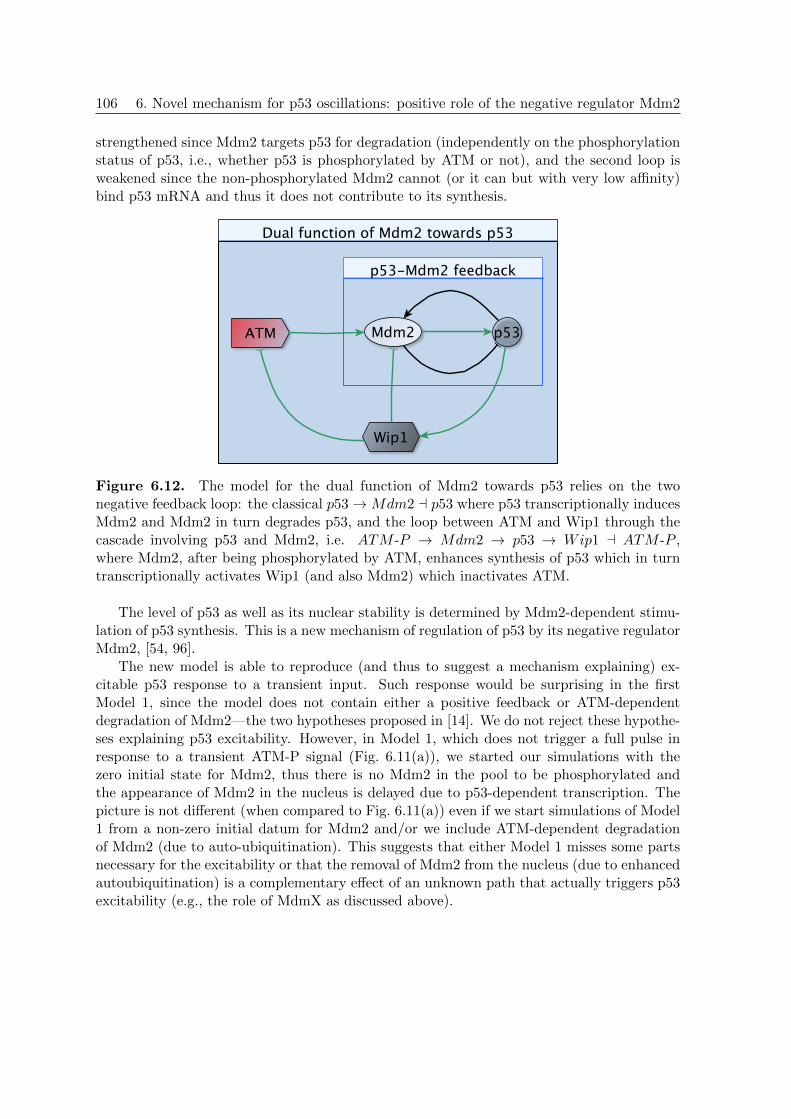
106 6. Novel mechanism for p53 oscillations: positive role of the negative regulator Mdm2
strengthened since Mdm2 targets p53 for degradation (independently on the phosphorylationstatus of p53, i.e., whether p53 is phosphorylated by ATM or not), and the second loop isweakened since the non-phosphorylated Mdm2 cannot (or it can but with very low affinity)bind p53 mRNA and thus it does not contribute to its synthesis.
Figure 6.12. The model for the dual function of Mdm2 towards p53 relies on the twonegative feedback loop: the classical p53→Mdm2 a p53 where p53 transcriptionally inducesMdm2 and Mdm2 in turn degrades p53, and the loop between ATM and Wip1 through thecascade involving p53 and Mdm2, i.e. ATM -P → Mdm2 → p53 → Wip1 a ATM -P ,where Mdm2, after being phosphorylated by ATM, enhances synthesis of p53 which in turntranscriptionally activates Wip1 (and also Mdm2) which inactivates ATM.
The level of p53 as well as its nuclear stability is determined by Mdm2-dependent stimu-lation of p53 synthesis. This is a new mechanism of regulation of p53 by its negative regulatorMdm2, [54, 96].
The new model is able to reproduce (and thus to suggest a mechanism explaining) ex-citable p53 response to a transient input. Such response would be surprising in the firstModel 1, since the model does not contain either a positive feedback or ATM-dependentdegradation of Mdm2—the two hypotheses proposed in [14]. We do not reject these hypothe-ses explaining p53 excitability. However, in Model 1, which does not trigger a full pulse inresponse to a transient ATM-P signal (Fig. 6.11(a)), we started our simulations with thezero initial state for Mdm2, thus there is no Mdm2 in the pool to be phosphorylated andthe appearance of Mdm2 in the nucleus is delayed due to p53-dependent transcription. Thepicture is not different (when compared to Fig. 6.11(a)) even if we start simulations of Model1 from a non-zero initial datum for Mdm2 and/or we include ATM-dependent degradationof Mdm2 (due to auto-ubiquitination). This suggests that either Model 1 misses some partsnecessary for the excitability or that the removal of Mdm2 from the nucleus (due to enhancedautoubiquitination) is a complementary effect of an unknown path that actually triggers p53excitability (e.g., the role of MdmX as discussed above).

6.4. Discussion and conclusions from the PDE model #2 107
Parameter Value [Units] Description
kub-1 5 [min−1] velocity of Mdm2-dep. ubiq. of p53-1, [78]
kub-2 1 [min−1] velocity of Mdm2-dep. ubiq. of p53-2, [est.]
Kub 1 [µM ] Michaelis rate of Mdm2-dep. ubiq. of p53, [78]
k?S 0.0005 [µM/min] basal synthesis rate of p53 mRNA, [est.]
ktp-1 1 [min−1] translation rate for p53-1, [16]
ktp-2 3 [min−1] translation rate for p53-2, [54, 96]
k?Sm 0.000005 [µM/min] basal synthesis rate of Mdm2 mRNA, [est.]
kSpm 0.03 [µM/min] velocity of Mdm2 mRNA transcription, [est.]
KSpm 10 [µM ] Michaelis rate of Mdm2 mRNA transcription, [est.]
ktm 1 [min−1] translation rate for Mdm2, [16]
k?Sw 0.000003 [µM/min] basal synthesis rate of Wip1 mRNA, [est.]
kSpw 0.03 [µM/min] velocity of Wip1 mRNA transcription, [est.]
KSpw 10 [µM ] Michaelis rate of Wip1 mRNA transcription, [est.]
ktw 1 [min−1] translation rate for Wip1, [16]
kph2 1 [min−1] velocity of ATM activation by E, [est.]
Kph2 0.3 [µM ] Michaelis rate of ATM activation by E, [est.]
kdph2 96 [min−1] velocity of Wip1-dep. deph. of ATM-P, [136]
Kdph2 26 [µM ] Michaelis rate of Wip1-dep. deph. of ATM-P, [136]
kph3 1 [min−1] velocity of ATM-dep. ph. of Mdm2, [est.]
Kph3 1 [µM ] Michaelis rate of ATM-dep. ph. of Mdm2, [est.]
kdph3 84 [min−1] velocity of Wip1-dep. deph. of Mdm2-P, [155]
Kdph3 23 [µM ] Michaelis rate of Wip1-dep. deph. of Mdm2-P, [155]
ka 20 [min−1] association rate for the complex C, [est.]
kd 0.01 [µM−1min−1] dissociation rate from the complex C, [est.]
E 1 [µM ] concentration of “the damage signal”, [chosen]
ATMTOT 1 [µM ] total ATM concentration, [chosen]
Table 6.2. Parameter values for the RD PDE system (6.3)-(6.4) modelling p53 dynamicswith a dual function of Mdm2 toward p53. Degradation terms are collected in Table 2.1. Inthe table, “dep.” stands for dependent, “ubiq.” for ubiquitination, “ph.” for phosphorylationand “deph.” for dephosphorylation.?The constant rates represent the total net production in a certain area of the cell: the basalrates kS , kSm and kSm produce substrates of the assigned values over the whole DNA locus.

108 6. Novel mechanism for p53 oscillations: positive role of the negative regulator Mdm2

7
Summary of the p53 modelling andfollow-up work
7.1 Physiological ODE and PDE models for p53
The aim of our modelling, rather simple compared with the overall complexity of p53 sig-nalling network in cell fate decisions between survival and death, is to simulate activationof p53 in single cells, the concentration of which shows sustained oscillations under stressconditions, the duration of oscillations being independent of the damage signal. Thus, wesimplified the p53 network by neglecting (hundreds of) possible target proteins and kept onlythose proteins that are actually experimentally justified to be necessary and sufficient foroscillations [15]. Therefore, four proteins, particularly, p53, Mdm2, Wip1 and ATM werechosen. Plausible effects of any positive feedback are not disputed in our work. We havedeveloped the compartmental ODE model which became basis for the two spatial RD PDEmodels simulating the p53 protein in a single cell in response to DNA DSB (caused by γ-radiation, cytotoxic drugs used in chemotherapy or by other means).
Basic features of the models are: compartmental distribution of the cellular processesbetween those occurring in the nucleus and those in the cytoplasm, the negative feedbackloop p53 → Mdm2 a 53 and then either the negative loop ATM → p53 → Wip1 a ATM(in the ODE model and the PDE Model 1) or ATM → Mdm2 → p53 → Wip1 a ATM(in the PDE Model 2 with the dual function of Mdm2). It was confirmed that the solep53-Mdm2 negative feedback is not sufficient for triggering oscillations. Instead, activationand regulation of p53 must involve the ATM and Wip1 proteins considered as continuoustime- and space-dependent (in the PDE models) functions, the dynamics of which is fullydescribed by mathematical equations rather than being represented by constant parameters.In our context, a special signal denoted by E acts as a transmitter of information aboutthe presence of the DNA DSBs; E is assumed to be a constant positively correlated withthe DNA damage dose. We assume that the higher doses a cell is exposed to, the biggernumber of DSB is caused, the stronger activation signal E is produced, and we have shownby the PDE models that the amplitudes and periods of p53 oscillations are, as expected fromexperiments, independent of the damage dose (that is independent of E).
In principle, one can similarly model intracellular pathways of any other proteins, i.e.,write as many reactions as necessary just by employing simple tools such as The Law of MassAction, Michaelis-Menten and Hill kinetics. Since the spatial representation of the signallingpathways can reveal diffusion-driven patterns that are hidden in ODE, we aimed to attractattention to reaction-diffusion equations. Our models are still simple since, in contrast to theODE setting, the spatial models are placed into a structural framework of the cell composed
109

110 7. Summary of the p53 modelling and follow-up work
of the two compartments only, nucleus and cytoplasm, and the diffusive motion of the speciesin and between these compartments is further considered. However, we believe that the PDEmodels are much more physiological than (rougher) ODE models since they are naturally ableto take intracellular spatial features into account including possible space heterogeneities inthe intracellular medium. For instance, the oscillatory patterns in the p53 concentrationare self-organised not only due to the reactions in the nucleus or in the cytoplasm but thatthey are also tightly connected to the boundary conditions on the membranes and to thediffusions of the species. The physiological delays maintained due to the semipermeabilityof the nuclear membrane are more typical for PDEs than for ODEs (if one does not want todeal with artificial delays represented by DDEs). The second specific property of the PDEmodels, which affects amplitudes, periods and the timing of pulses, is diffusive motion ofthe species. Although, we were able to find some lower bounds for the diffusion coefficients,below which we do not receive any oscillations, oscillations can be maintained for any otherdiffusions larger than these bounds. One may expect such results since fast diffusions makesolutions of the RD system homogenous in space and thus, roughly speaking, the PDE systemresembles the compartmental ODE model which describes the dynamics of proteins with thesame reaction terms and thus it is able to produce oscillations in the p53 concentration.
Further, intracellular signalling in our modelling setting is restricted to the cells of physiol-ogy and morphology where a molecular network in question is, at least, partially understood.What does the p53 signal transduction in response to DNA damage in a nerve cell or in apolynucleic muscle cell look like? What is the role of diffusion in a cell where a signal isspread over long distances and in very small cells? These and other questions should befurther addressed and spatial PDE models might fruitfully be used for this purpose.
Reaction-diffusion systems could be thus considered as an alternative approach to classicalODEs which may put some light on protein signalling and will be of some help to biologists andmodellers who want to describe intracellular spatio-temporal dynamics of proteins in a faithfulyet more demanding (in terms of parameter estimation) way. Such reaction-diffusion PDEmodels are also amenable to describe spatio-temporal dynamics at the level of cell populationsand that, by introducing intercellular signalling, it is in principle possible to connect the twoobservation levels. This perspective still remains a challenge to mathematicians and modellersin biology.
7.2 p53 as a chemotherapeutic target
The protein p53 is a well studied protein due to its role in the protection of the genome.Furthermore, because p53 can elicit life or death decisions in cells, it has recently become atherapeutic target in cancer treatment. Therapeutic effort in p53-aimed treatments focusesmainly on either substitution of the p53 lost functionality and destabilisation of oncogenic p53mutants or restoration of p53 function by targeting upstream proteins in the p53 signallingpathway, in particular the negative regulators Mdm2 and Wip1 which, in some cancer cells,are over-expressed and thus suppress the p53 functionality, see [66, 79] and citations therein.
There have been developed and already used in clinical testing several protocols and p53-based anti-cancer therapies including retrovirus- or adenovirus-mediated gene therapy (torestore p53 function), targeting p53-deficient cells with modified adenoviruses, pharmacolog-ical modulation of p53 (and also p63 and p73) protein functions, identification and designof small-molecule inhibitors of the Mdm2-p53 (and Wip1-p53) interactions (potential thera-peutic agents: nutlins, RITA, spiro-oxindoles, quinolinols). However, there are not yet clearclinical studies confirming successful applications of the therapies in the treatment of cancers.In addition, the described therapeutic efforts were accompanied with unwanted side effects
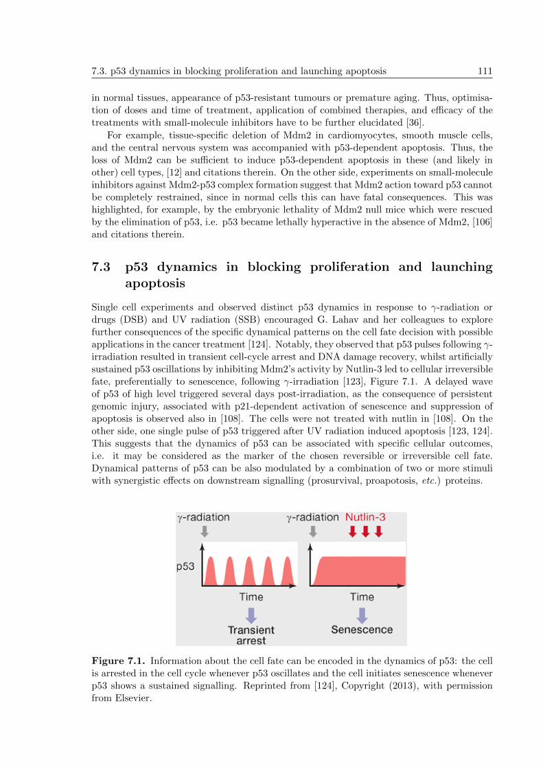
7.3. p53 dynamics in blocking proliferation and launching apoptosis 111
in normal tissues, appearance of p53-resistant tumours or premature aging. Thus, optimisa-tion of doses and time of treatment, application of combined therapies, and efficacy of thetreatments with small-molecule inhibitors have to be further elucidated [36].
For example, tissue-specific deletion of Mdm2 in cardiomyocytes, smooth muscle cells,and the central nervous system was accompanied with p53-dependent apoptosis. Thus, theloss of Mdm2 can be sufficient to induce p53-dependent apoptosis in these (and likely inother) cell types, [12] and citations therein. On the other side, experiments on small-moleculeinhibitors against Mdm2-p53 complex formation suggest that Mdm2 action toward p53 cannotbe completely restrained, since in normal cells this can have fatal consequences. This washighlighted, for example, by the embryonic lethality of Mdm2 null mice which were rescuedby the elimination of p53, i.e. p53 became lethally hyperactive in the absence of Mdm2, [106]and citations therein.
7.3 p53 dynamics in blocking proliferation and launchingapoptosis
Single cell experiments and observed distinct p53 dynamics in response to γ-radiation ordrugs (DSB) and UV radiation (SSB) encouraged G. Lahav and her colleagues to explorefurther consequences of the specific dynamical patterns on the cell fate decision with possibleapplications in the cancer treatment [124]. Notably, they observed that p53 pulses following γ-irradiation resulted in transient cell-cycle arrest and DNA damage recovery, whilst artificiallysustained p53 oscillations by inhibiting Mdm2’s activity by Nutlin-3 led to cellular irreversiblefate, preferentially to senescence, following γ-irradiation [123], Figure 7.1. A delayed waveof p53 of high level triggered several days post-irradiation, as the consequence of persistentgenomic injury, associated with p21-dependent activation of senescence and suppression ofapoptosis is observed also in [108]. The cells were not treated with nutlin in [108]. On theother side, one single pulse of p53 triggered after UV radiation induced apoptosis [123, 124].This suggests that the dynamics of p53 can be associated with specific cellular outcomes,i.e. it may be considered as the marker of the chosen reversible or irreversible cell fate.Dynamical patterns of p53 can be also modulated by a combination of two or more stimuliwith synergistic effects on downstream signalling (prosurvival, proapotosis, etc.) proteins.
Figure 7.1. Information about the cell fate can be encoded in the dynamics of p53: the cellis arrested in the cell cycle whenever p53 oscillates and the cell initiates senescence wheneverp53 shows a sustained signalling. Reprinted from [124], Copyright (2013), with permissionfrom Elsevier.

112 7. Summary of the p53 modelling and follow-up work
A stressed cell likely evaluates the presence of both proarrest and proapoptotic proteinsproduced in a p53-dependent manner at any time during its response to DNA damage.The cell determines the so-called “apoptotic ratio”1 with respect to protein concentrations,duration of their expression and other factors. Irreversible apoptosis is initiated wheneverthis ratio crosses a given threshold [73]. Expression of those apoptosis-launching proteins iscomplex process that depends on many factors (post-translational modifications, interactionswith other cellular substrates, location). On the other side, it is observed that p53, itsregulators and most of the apoptotic proteins are all short-lived proteins [106, 26]. Thismay suggest that these proteins exhibit a similar oscillatory behaviour in the (transient) cellcycle arrest and DNA damage repair, which does not allow them to accumulate sufficientlyto cross the apoptotic ratio. In contrast, p53 switched to the sustained signalling may lead tosufficient accumulation and stabilisation of apoptotic agents which are then able to initiateapoptotic program. Although further studies have to be done in this line, it seems, however,that the dynamics of p53 could control the apoptotic threshold of individual cells in responseto DNA damage. In this context, the oscillatory dynamics of the involved proteins can bepossibly explained as a periodical testing of the presence of DNA damage: if unrepaired DNADSB still exist, additional pulses of both phosphorylated ATM and p53 are triggered [15].
In an even more realistic vision of the processes leading a single cell to decision betweensurvival and death, more than deterministic events, random molecule encounters and stochas-tic gene expression should be taken into consideration, and should be modelled by stochasticprocesses (as sketched in [141] for Hes1), from which deterministic equations (partial dif-ferential equations physiologically structured in variables, identified as biological “readouts”in a single cell model, representing relevant biological variability inside the cell population)should be further designed at the level of cell populations.
In the same way, in the perspective of connecting the proposed p53 modelling with ex-isting PK–PD models, drug effects, measured only at the cell population level, can be rep-resented as environmental factors exerting their influence on molecular targets, included asfunctions in stochastic processes, at the level of a single cell. Establishing such connectionsbetween stochastic events at the individual cell level and resulting deterministic effects at thecell population level is a challenge for mathematical modelling that we intend to tackle infuture works. Readers interested in such interconnections between stochastic and determin-istic mathematics in the Hes1 regulatory network are recommended to read the papers byM. Sturrock et al. [141, 140] to get acquainted with this challenge.
7.4 Cancer therapies and PK–PD models
Most cytotoxic and cytostatic drugs used in cancer treatments act in a selective manner,taking advantage of differences in tumour cell characteristics, compared to healthy cells,such as high proliferation rates, genome instability and tolerance to hypoxia. This resultsin proper targeting of chemotherapeutic agents on tumour cells. However, cancer therapiesalso have toxic side effects on healthy cells and can lead to the disruption of physiologicalfunctionality of tissues and organs. In the particular case of chronotherapeutic settings (i.e.,hypothesising best treatment periods in the 24 hour span), physiologically based molecularpharmacokinetic-pharmacodynamic (PK–PD) models using ODEs have been proposed forthe cytotoxic drugs Oxaliplatin [30], 5-Fluorouracil [30, 87] and Irinotecan [9, 8], all threedrugs that are commonly used in the treatment of metastatic colorectal cancer. Moreover, tominimise such unwanted effects in more general (non chronotherapeutic) settings, most anti-
1The ratio which does not have to be necessarily associated with apoptosis but rather with any irreversiblecell fate.

7.5. Other concluding notes 113
cancer drugs are delivered in the clinic in time interval-depending regimens to allow cells torecover their normal functions after pharmacological insult. However, time intervals betweenchemotherapy courses also allow tumour cells to recover, activating their survival mecha-nisms, and further resist subsequent therapeutic insults. Optimal scheduling strategies arecurrently being theoretically investigated [29, 30, 19] to obtain satisfying trade-offs betweenthe objective of reducing the tumour burden without inducing neither intolerable side effectson healthy cells nor emergence of resistant clones in the tumour cell population.
Besides toxic side effects on healthy cells, tumour cells can indeed often develop multipleresistance to drugs. Moreover, in vivo observations in the tumour stromal tissue surroundingtumours of prostate, breast and ovary reveal the drug-induced production of a spectrumof secreted cytokines and growth factors, e.g., WNT16B, that promote tumour growth andsurvival of cancer cells after cytotoxic therapy, and further reduce chemotherapy sensitivityin tumour cells, resulting in tumour progression; otherwise said, among other constraints, onemust take into account the fact that chemotherapy itself can positively influence the growthof tumours [144].
In order to take into account these different therapy-limiting constraints, optimal admin-istration of anticancer agents should involve accurately representing the action of drugs at themolecular, i.e., intracellular, level, which means molecular PK–PD modelling for each drugused in a given treatment firstly at the level of a single cell and secondly at the level of cellpopulations, i.e., tissues and organs. The review of p53 molecular mechanisms of action, andtheir modelling, is positioned in continuity with, but downstream of, the action of cytotoxicanticancer drugs, when DNA damage is constituted, so that DNA damage is the interfacebetween molecular PK–PD models and the models we proposed in the thesis.
7.5 Other concluding notes
The oscillatory dynamics of p53, “the guardian of the genome”, has long been evidenced bybiological recordings in experimental conditions representing cell stress due to, e.g. radiotoxicinsult [77, 56]. In this sense, the biological question of identifying intracellular spatio-temporaldynamics is certainly crucial. Furthermore, since p53 disruptions are found in more than 50%of solid tumours, with various modifications of its stress-induced dynamics [149, 150, 111], itis also a crucial point in cancer therapy modelling to understand how p53 dynamics may beaffected in disease, and to this aim, to have an accurate representation of how p53 is activatedand regulated in physiological conditions, which was undertaken by our models.

114 7. Summary of the p53 modelling and follow-up work

Part II
Modelling enzyme reaction
115

8
Beyond the enzyme reaction model
As we have seen in the previous chapters, post-translational modifications (protein-protein interactions) can be modelled as the enzyme reactions, even though none ofthe proteins in question is a real enzyme. The Law of Mass Action (LMA) andparticularly the quasi-steady state approximation (QSSA) can be used to reduce fourequations for the species up to one composed of Michaelis function with two unknownparameters. These parameters can be sometimes found in the literature. In general,responses to a variety of stimuli consist of chains of successive protein interactionswhere enzymes play significant roles, mostly by speeding up reactions. Enzymes arecatalysts that convert other molecules (proteins) called substrates into products, butthe enzymes are not changed by the reaction [68]. In this chapter we deal with fewmathematical problems related to the enzyme reaction.
Organisation of the chapter is as follows: A brief introduction to the enzyme reactionis given first in Section 8.1. It is followed by Section 8.2 where we review the QSSAand give a proof of its validity in the ODE case. Finally, Section 8.3 deals withthe large-time behaviour of a reaction-diffusion system for the reversible enzymereaction.
8.1 Introduction to enzyme reactions
In the reaction scheme proposed by Michaelis and Menten in 1913 [107], the enzyme Econverts the substrate S into the product P through a two step process, schematically writtenas
S + Ek+
k−C
kp+−→ E + P, (8.1)
where C is the intermediate complex. Briggs and Haldane proposed in 1925 an ODE analysisof (8.1) which is now basis for the most current descriptions of enzyme reaction [21]. In theirquasi-steady state approximation (QSSA), the complex is assumed to reach its steady statequickly. Thus by setting dnC/dt ≈ 0 in the equation for the complex concentration nC = [C],the analysis ends up with an algebraic expression (i.e., Michaelis function) for nC and asimple (although nonlinear) equation for the substrate nS = [S] (called as Michaelis-Mentenequation). The kinetics of enzyme reaction described by Briggs and Haldane is sometimescalled Michaelis-Menten kinetics. A detailed analysis based on perturbation technique isfurther provided by Segel and Slemrod [133].
Importantly, P can also combine with E to form the complex C in (8.1), in fact, nearlyall enzymes increase the speed of the reaction in both directions [68], which is schematically
117

118 8. Beyond the enzyme reaction model
written as
S + Ek+
k−C
kp+kp−
E + P. (8.2)
The following two sections present two mathematical results related an ODE system for (8.1)in Section 8.2 and a reaction-diffusion PDE system for (8.2) in Section 8.3.
8.2 Michaelis-Menten Law and ODE system
In the framework of the irreversible enzyme reaction (8.1), the Law of Mass Action gives fourequations for the concentrations of species nS = [S], nE = [E], nC = [C] and nP = [P ], i.e.
dnSdt
= k−nC − k+nSnE ,dnEdt
= (k− + kp+)nC − k+nSnE ,
dnCdt
= k+nSnE − (k− + kp+)nC ,dnPdt
= kp+nC ,
(8.3)
where, for simplicity, the initial conditions (nS(0), nE(0), nC(0), nP (0)) = (n0S , n
0E , 0, 0) are
assumed.The last equation for the product P is uncoupled from the others and it can be thus
omitted from further considerations. In addition, two conservation laws hold, particularly,nE + nC = n0
E and nS + nC + nP = n0S . Using the former one, we can reduce the above
equations intodnSdt
= k−nC − k+nS(n0E − nC), (8.4)
dnCdt
= k+[nS(n0E − nC)−KmnC ], (8.5)
where Km =k− + kp+
k+is the Michaelis constant.
After a transient pre-steady-state phase (where the depletion of nS is assumed to be neg-
ligible), one can observe thatdnCdt
= 0 that is indeed true whenever the concentration of
enzyme is small enough compared to the concentration of the substrate (where free enzymemolecule is immediately bound to another substrate molecule). Thus, in the standard QSSA(sometimes referred to as Michaelis-Menten law), we can replace the equation of the fast vari-able (complex), which reaches its equilibrium quickly, by an algebraic formula. In particular,we can write1
dnSdt
= k−nC − k+nS(n0E − nC), (8.6)
0 = k+[nS(n0E − nC)−KmnC ], (8.7)
and in a more condensed way,dnSdt
= −kp+nC (8.8)
where
nC = n0E
nSKm + nS
. (8.9)
Note that the assumption on negligible depletion of the initial concentration of nS in thepre-steady state phase becomes important when we set nS(0) = nS(0) = n0
S .
1The different notation for the concentrations used in the following equations (8.6), (8.7) and so on, e.g.,nS and nC , is a matter of convenience only. In the proof of validity of the QSSA, we will need to distinguishbetween the “pre-QSSA” solution to (8.3) and “post-QSSA” solution to (8.6) and (8.7).
8.2. Michaelis-Menten Law and ODE system 119
We prove the following
Proposition 8.1 (Validity of the QSSA). For n0E small there is a constant C = C(n0
S)independent of n0
E such that
supt≥0|nS(t)− nS(t)| ≤ Cn0
E . (8.10)
Remark 8.2. To prove this result, one can introduce a scaling as in [119], i.e.
ε = n0E , s = εt, uS(s) = nS(t) and uC(s) =
nC(t)
ε.
However, different scalings can be also found in the literature when the system (8.4)-(8.5) isstudied, e.g., the scaling of Heineken et al. [63] (which is also used in the book of Keener &Sneyd [68]) and Segel & Slemrod’s scaling [133], which is based on a detailed analysis of theduration of pre- and steady-state phases. For the convenience, they are summarised in thefollowing table,
ε = n0E s = εt uS(s) = nS(t) uC(s) =
nC(t)
εin [119],
ε =n0E
n0S
s = k+n0Sεt uS(s) =
nS(t)
n0S
uC(s) =nC(t)
εn0S
in [63],
ε =n0E
Km + n0S
s = kp+εt uS(s) =nS(t)
n0S
uC(s) =nC(t)
εn0S
in [133].
By applying any of these scalings, one can reduce the system (8.4)-(8.5) to a slow-fastdynamics. Note, however, that the small parameter ε of Segel & Slemrod [133] allows alsosituation where n0
E does not have to be necessarily smaller than n0S. In such case, the complex
concentration nC must be smaller than nS (i.e., Km must be large enough). Although, Segel& Slemrod’s condition n0
E Km + n0S validates the enzyme dynamics for more initial states
than the experimental condition n0E n0
S, it still does not cover all possible initial states.
Proof. To cover all the three scalings, we can define
ε =n0E
α, s = βεt, uS(s) =
nS(t)
γand uC(s) =
nC(t)
δε(8.11)
for α, β, γ, δ > 0 constants2 Using (8.11), the equations can be rescaled to
duSds
=k−δ
βγuC −
k+
βuS(α− δuC), (8.12)
εduCds
=k+
βδ[γuS(α− δuC)−KmδuC ], (8.13)
with the initial conditions (uS(0), uC(0)) = (n0S/γ, 0), and
duSds
=k−δ
βγuC −
k+
βuS(α− δuC), (8.14)
2Thus, α = β = γ = δ = 1 in [119]; α = n0S , β = k+n
0S , γ = δ = n0
S in [63]; and α = n0S + Km, β = kp+,
γ = δ = n0S in [133]).

120 8. Beyond the enzyme reaction model
0 =k+
βδ[γuS(α− δuC)−KmδuC ], (8.15)
with the initial condition uS(0) = n0S/γ. From (8.13), we can write
uC =α
δ
γuSγuS +Km
andduSds
= −kpα
β
uSγuS +Km
. (8.16)
Thus, instead of (8.10) we prove
sups≥0|uS(s)− uS(s)| ≤ Cε. (8.17)
Note, that when we compare equations in (8.16) we can obtain
duSds
= −kpδ
βγuC , (8.18)
the relation, that can be also immediately obtained by combining (8.14)+δ/γ(8.15). We canalso notice that
d
ds(uS + ε
δ
γuC) = −kp
δ
βγuC . (8.19)
Further, it is not difficult to see that both pairs uS , uS and uC , uC are non-negative andbounded from above. Precisely, 0 ≤ uS(s) ≤ n0
S/γ, 0 ≤ uS(s) ≤ n0S/γ 0 ≤ uC(s) ≤ α/δ and
0 ≤ uC(s) ≤ α/δ. In fact,
uC(s), uC(s) ≤ uM , where uM =α
δ
n0S
n0S +Km
.
For z(s) =duCds
(s) we can write equation εdz
ds+λ(s)z(s) = µ(s)z(s) where µ is bounded and
λ(s) =k+
β(γuS +Km) ≥ k+
βKm, which implies boundedness of z, i.e. we can find a constant
K such that
∣∣∣∣duCds
∣∣∣∣ ≤ K.
Finally, using the properties above, we can show that R(s) = uS(s) + εδ
γuC(s)− uS(s) is
bounded, i.e. |R(s)| ≤ Cε for some constant C, from where (8.17) follows.
To prove boundedness of R, let us define r(s) = −βδ
duCds
+ k+u2C bounded. Multiplying
R by k+uC and r by εδ
γyields, after some necessary calculations,
uC =εδr − k+γuCR+ k+αγ/δuS
k+(γuS +Km),
and (using (8.16) and uS − uS from the definition of R)
uC − uC =εδr − k+γ(
α
δ− uC)R− εk+αuC
k+(γuS +Km).
Thus, using (8.18) and (8.19), we obtain
dR
ds=
d
ds(uS + ε
δ
γuC)− d
dsuS = −kp
δ
βγ(uC − uC),

8.3. Reaction-diffusion system for the reversible enzyme reaction 121
and, after rearranging the terms, we have
dR
ds+ kp
δ
β
α/δ − uCγuS +Km
R = εkpδ
βγ
(−δ/k+r + αuCγuS +Km
).
and thus R bounded.
Note that this proof written for a specific choice of α = β = γ = δ = 1 can be found inthe lecture notes of B. Perthame [119].
8.3 Reaction-diffusion system for the reversible enzyme reac-tion
The entire mathematical treatment of the enzyme reactions (8.1) and (8.2) is usually done byusing ODEs. However, protein pathways occur in living cells, heterogenous spatial structureof which has an impact on the reaction efficiency, speed of the enzyme reaction and conver-gence to the respective equilibria. In the sequel, a reaction-diffusion system for the reversibleenzyme reaction (8.2) is studied.
More precisely, by employing the LMA we obtain four equations which, equipped with theLaplacians for the diffusive motion of the species, describe the concentrations of the speciesin (8.2) in time and space. These equations are, respectively,
∂nS∂t−DS∆nS = k−nC − k+nSnE ,
∂nE∂t−DE∆nE = (k− + kp+)nC − k+nSnE − kp−nEnP ,
∂nC∂t−DC∆nC = k+nSnE − (k− + kp+)nC + kp−nEnP ,
∂nP∂t−DP∆nP = kp+nC − kp−nEnP ,
(8.20)
where ni, i ∈ S,E,C, P, are the concentrations of the substrate S, enzyme E, intermediatecomplex C and product P . It is assumed that ni = ni(t, x) are defined on an open boundeddomain Ω with sufficiently smooth boundary and a time interval I = [0, T ] for 0 < T < ∞,QT = I ×Ω. Without loss of generality we will assume |Ω| = 1. Diffusion coefficients Di areassumed to be positive and different from each other. Further we assume that there existnon-negative functions n0
i such that
ni(0, x) = n0i (x),
ˆΩn0i (x) dx > 0, ∀ i ∈ S,E,C, P. (8.21)
Finally, the system is coupled with the zero-flux boundary conditions
ν · ∇ni = 0, ∀t ∈ I, x ∈ ∂Ω, i ∈ S,E,C, P, (8.22)
where ν is a unit normal vector pointed outward from the boundary ∂Ω.The species in the reaction (8.2) are conserved in the following way:
0 < M1 =
ˆΩ
(nE + nC)(t, x) dx =
ˆΩ
(n0E + n0
C)(x) dx ∀t ≥ 0, (8.23)
0 < M2 =
ˆΩ
(nS + nC + nP )(t, x) dx =
ˆΩ
(n0S + n0
C + n0P )(x) dx ∀t ≥ 0, (8.24)

122 8. Beyond the enzyme reaction model
with the total mass M = M1 +M2.
The conservations of masses (8.23) and (8.24) give L1-bounds on the solutions of thereversible enzyme reaction system (8.20)-(8.22) uniformly in time. This is unfortunatelyinsufficient to show the existence of solutions on I = [0, T ] for any T <∞. Global existenceof a weak solution of system (8.20)-(8.22) is a consequence of a combination of the dualityargument (Appendix A), which provides L2-estimates on the nonlinearities of the system(which are at most quadratic), and an “approximation method” of M. Pierre [120, 122, 40],which justifies rigorously the existence of the solutions of (8.20)-(8.22) (which are build upfrom the solutions of the approximated system). The existence of a global weak solutionwith the total mass conserved in the way as in (8.23) and (8.24) can also be showed by theRothe method, which provides a constructive proof and thus it can be also used in numericalsimulations, see Appendix B.
Here we prove the following
Proposition 8.3. Let n0i ∈ L2(logL)2(Ω), then any weak solution ni, i ∈ S,E,C, P
to (8.20)-(8.22) with the conserved mass according to (8.23) and (8.24) belongs to L2(QT )for each T <∞. In particular, by a duality argument we obtain
‖ni(log(σini)− 1)‖L2(QT ) ≤ C(1 + T )∥∥∥ ∑i∈S,E,C,P
n0i (log(σin
0i )− 1)
∥∥∥L2(Ω)
,
cf. (8.33) below, where σi are constants dependent on the kinetic rates kj given by (8.27).
If in addition to the L2-estimates arising from Proposition 8.3 the solution ni of (8.20)-(8.22) satisfies uniform L∞-bounds, we can deduce global existence in time of “classical”(strong) solutions3, by the standard results for reaction-diffusion systems4, i.e. we can showthe smoothness of ni (e.g., ni ∈ C2([0, T ] × Ω) or ni ∈ C∞([0, T ] × Ω), for any T < ∞) forall smooth non-negative initial data, depending on the regularity of the boundary ∂Ω (being,respectively, C2+α or C∞). By using the properties of the heat kernel (c.f., Lemma 8.8)combined with a bootstrapping argument we can indeed prove
Proposition 8.4. Let n0i ∈ L∞(Ω), then ni ∈ L∞loc([0,∞) × Ω) (locally in time), i ∈
S,E,C, P.
The large time behaviour of the solution ni, i ∈ S,E,C, P, of the system (8.20)-(8.22)is studied by means of the relative entropy convergence. As the main result we prove
Theorem 8.5. Let ni be a solution to the system (8.20)-(8.22) satisfying the conservationlaws (8.23) and (8.24). Then there exist two constants C1 and C2 such that∑
i∈S,E,C,P
‖ni − ni,∞‖2L1(Ω) ≤ C2e−C1t
cf. (8.51) below, where ni,∞ are unique positive steady-states to (8.20)-(8.22) definedin (8.35).
3By classical solution we mean bounded solution, so that, by a regularity theory, a classical solution hasclassical derivatives at least a.e. and the equations (8.20) are understood pointwise.
4Smoothness is an easy consequence of general properties of the heat operator and the regularity withrespect to a parameter of solutions of ODEs [38], p.11-12.
8.3. Reaction-diffusion system for the reversible enzyme reaction 123
8.3.1 Entropy, entropy dissipation and first estimates
Let us first mention a simple result on the non-negativity of solutions to (8.20)-(8.22). Itfollows from the so-called quasi-positivity property of the right hand sides of (8.20). Inparticular, it can be proved
Lemma 8.6. For n0i (x) ≥ 0 in Ω, a solution ni of the system (8.20)-(8.22) is non-negative
for t ∈ I and x ∈ Ω, i = S,E,C, P, i.e.
ni(t, x) ≥ 0 everywhere in QT .
Proof. The r.h.s. of (8.20), denoted here by fi = fi(nS , nE , nC , nP ), i ∈ S,E,C, P, satisfiesthe quasi-positivity property, i.e. fi(ni = 0) ≥ 0 for each i ∈ S,E,C, P, which implies thenon-negativity of the solution, see, e.g., [121].
For the species ni, i ∈ S,E,C, P, we will sometimes write shortly n = (nS , nE , nC , nP ).The entropy functional E(n) : [0,∞)4 → [0,∞) and entropy dissipation D(n) : [0,∞)4 →[0,∞) are defined, respectively, by
E(n(t, x)) =
ˆΩ
∑i=S,E,C,P
ni(log(σini)− 1) + 1/σi dx (8.25)
where σS , σE , σC and σP are constants dependent on the kinetic rates kj to be determined,and
D =
ˆΩ
∑i=S,E,C,P
Di|∇ni|2
nidx
+
ˆΩ
[(k+nSnE − k−nC) (log(σSσEnSnE)− log(σCnC))
+ (kp−nEnP − kp+nC) (log(σEσPnEnP )− log(σCnC))] dx.
(8.26)
Note that the function x log(x) − x + 1 is non-negative and strictly convex on [0,∞).Thus, E is non-negative as well for any t ≥ 0. The dissipation D is also non-negative for allt ≥ 0 and for any α, β > 0 such that
σC = αk−, σSσE = αk+,
σC = βkp+, σEσP = βkp−.(8.27)
The non-negativity of D follows from the trivial inequality (x − y)(log x − log y) ≥ 0 valid
for all x, y ∈ R. For example, we can choose α = 1, β =k−kp+
, σC = σE = k−, σS =k+
k−and
σP =kp−kp+
in (8.27).
It is straightforward to verify that D = −dE
dt, which implies that E is decreasing as a
function of the time t and that the limit limt→∞
E(n(t, x)) exists. By integrating this simple
relation over [t1, t2] (t2 > t1 > 0) we obtain,
E(n(t1, x))− E(n(t2, x)) =
ˆ t2
t1
D(n(s, x))ds
which implies
limT→∞
ˆ ∞T
D(n(s, x))ds = 0.

124 8. Beyond the enzyme reaction model
From above, we can also write
E(n(t, x)) +
ˆ t
0D(n(s, x))ds = E(n(0, x)). (8.28)
From the definitions of entropy and entropy dissipation, by using their non-negativitiesand (8.28), we can deduce the following a-priori estimates for each species ni, i ∈ S,E,C, P:
supt∈[0,∞)
‖ni log(ni)‖L1(Ω) ≤ C, (8.29)
i.e., ni ∈ L∞([0,∞);L(logL)(Ω)); and using|∇ni|2
ni= 4|∇√ni|2 we deduce
‖∇√ni‖2L2([0,∞);L2(Ω;Rd)) ≤ C, (8.30)
i.e.,√ni ∈ L2([0,∞);W 1,2(Ω)). In all these estimates C = E(n(0, x) independent of the
time.The conservation laws (8.23) and (8.24) imply L1(Ω)-bounds for ni for all t ≥ 0, that is
ni ∈ L∞([0,∞);L1(Ω)) (and also trivially√ni ∈ L∞([0,∞);L2(Ω))), i ∈ S,E,C, P.
8.3.2 L2(logL)2 estimates
Proposition 8.3 states the L2(logL)2 estimate for ni. This proposition can be proved by aduality argument of M. Pierre [122, 121] , see Appendix A, applied to the system (8.20)-(8.22).We obtain the following
Proof. (of Proposition 8.3) The system (8.20)-(8.22) can be rewritten in the terms of thenon-negative entropy density variables zi = ni(log(σini)− 1) + 1/σi to the form
∂z
∂t−∆(Az) ≤ 0, ν · ∇(Az) = 0 (8.31)
where z =∑zi, zd =
∑Dizi (sums go for i ∈ S,E,C, P) and A = zd/z ∈
[D,D
]for
D = mini∈S,E,C,PDi and D = maxi∈S,E,C,PDi. Indeed, after some calculation, wearrive to
∂z
∂t−∆(Az) =−
∑Di|∇ni|2
ni− (k+nSnE − k−nC) (log(σSσEnSnE)− log(σCnC))
− (kp−nEnP − kp+nC) (log(σEσPnEnP )− log(σCnC)) .
(8.32)
The right hand side of (8.32) is non-positive for σi as in (8.27), i.e. for σi which satisfy
σC = αk−, σSσE = αk+,
σC = βkp+, σEσP = βkp−,
for some α, β > 0. The boundary condition in (8.31) is easy to be verified.A duality argument, Lemma 8.18 from Appendix A, applied to (8.31) implies the estimate
‖ni(log(σini)− 1)‖L2(QT ) ≤ C(1 + T )∥∥∥ ∑i∈S,E,C,P
n0i (log(σin
0i )− 1) +
1
σi
∥∥∥L2(Ω)
, (8.33)
which we wanted to prove.
Remark 8.7. Thus, ni ∈ L2(logL)2(QT ) whenever n0i ∈ L2(logL)2(Ω). Finally, since
L2(logL)2(QT ) ⊂ L2(QT ) for Ω bounded and T < ∞ (because of the trivial inequalityx log x ≥ x− 1), there is a constant C dependent on the time T such that ‖ni‖L2(QT ) ≤ C(T )for each i ∈ S,E,C, P.
8.3. Reaction-diffusion system for the reversible enzyme reaction 125
8.3.3 L∞ estimates in 1-3D: bootstrapping argument
A bootstrapping argument5 combined with the smoothing properties of the heat kernel (cf.Lemma 8.8) are used to show L∞ bounds for the weak solution ni ∈ L2(QT ) of the sys-tem (8.20)-(8.22) in the space dimensions d = 1, 2 and 3. The smoothing property of theheat kernel in question can be stated as follows (see also [38]):
Lemma 8.8. Consider f = f(t, x) ∈ Lp(QT ) and u = u(t, x) a solution of
∂tu−∆u = f, ∀t ∈ I, x ∈ Ω,
ν · ∇u = 0, ∀t ∈ I, x ∈ ∂Ω,
u(0, x) = u0(x) ∈ L∞(Ω).
Then it holds that u ∈ Lq(QT ) for all q ∈ [1,∞] satisfying
1
q>
1
p− 2
d+ 2. (8.34)
With this lemma in hand, we can proceed with the proof of Proposition 8.4.
Proof. (of Proposition 8.4) Since the system (8.20) satisfies
∂nS∂t−DS∆nS ≤ k−nC ,
∂nE∂t−DE∆nE ≤ (k− + kp+)nC ,
∂nC∂t−DC∆nC ≤ (k+nS + kp−nP )nE ,
∂nP∂t−DP∆nP ≤ kp+nC ,
then, for uC ∈ L2loc([0,∞) × Ω) (locally in time), the property of the heat kernel (8.34)
implies nS , nP ∈ Lq0loc([0,∞)× Ω) for all q0 such that1
q0>
1
2− 2
d+ 2=
d− 2
2(d+ 2). Applying
Holder inequality with nE ∈ L2loc([0,∞)×Ω) and nS , nP ∈ Lq0loc([0,∞)×Ω), we have (k+nS +
kp−nP )nE ∈ Lr0loc([0,∞) × Ω) for1
r0>
d
d+ 2. As a consequence, the property of the heat
kernel (8.34) gives nC ∈ Ls0loc([0,∞) × Ω) for1
s0>
1
r0− 2
d+ 2>
d− 2
d+ 2. Finally, nE ∈
Ls0loc([0,∞)× Ω) for the same s0.
Thus, by the property of the heat kernel only (no bootstrapping is needed here), we obtainnS , nP ∈ Lq0loc([0,∞)×Ω) for q0 ∈ [1,∞) and nC , nE ∈ Ls0loc([0,∞)×Ω) for s0 ∈ [1,∞) in thesimpler cases of d = 1, 2.
For d = 3, we apply a bootstrapping argument combined further with the property of theheat kernel (8.34). We can deduce from above that nS , nP ∈ Lq0loc([0,∞)×Ω) for q0 ∈ [1, 10),(k+nS + kp−nP )nE ∈ Lr0loc([0,∞) × Ω) for r0 ∈ [1, 5/3), and nC , nE ∈ Ls0loc([0,∞) × Ω) fors0 ∈ [1, 5). Since ∂tnS − DS∆nS ≤ k−nC ∈ Ls0 and ∂tnP − DP∆nP ≤ kp+nC ∈ Ls0 , we
have nS , nP ∈ Lq1loc([0,∞)×Ω) for q1 such that1
q1>
1
s0− 2
5> −1
5, i.e. for q1 ∈ [1,∞]. As a
consequence, (k+nS + kp−nP )nE ∈ Lr1loc([0,∞)×Ω) for1
r1>
1
5, and so nC ∈ Ls1loc([0,∞)×Ω)
5A bootstrapping argument, as it is used here, has been adapted from [38].

126 8. Beyond the enzyme reaction model
for1
s1>
1
r1− 2
5> −1
5, i.e., for all s1 ∈ [0,∞]. Finally, since ∂tnE−DE∆nE ≤ (k−+kp+)nC ∈
Ls1 , then also nE ∈ Ls1loc([0,∞)× Ω) for s1 ∈ [0,∞].
Thus, in the dimensions d = 1, 2 and 3, we have ni ∈ L∞(QT ) for any T <∞6.
Note that we can proceed in a similar way to show L∞ bounds for higher space dimensions.For more details, see [38].
By using simple arguments it can be easily shown that ‖∇ni‖L2(QT ) ≤ C and thus wealso have ni ∈W 1,2(Ω) for each t ∈ I.
8.3.4 Other properties of the EnR system
Let us also observe that for the positive diffusivities Di, the system (8.20)-(8.22) possesses aunique constant steady state n∞ = (nS,∞, nE,∞, nC,∞, nP,∞).
Lemma 8.9. For M = M1 +M2 and K =k−k+
+kp+kp−
, the system (8.20)-(8.22) has a unique
constant strictly positive steady state n∞,
nC,∞ =1
2
(M +K −
√(M +K)2 − 4M1M2
),
nE,∞ = M1−nC,∞, nS,∞ =k−nC,∞k+nE,∞
, nP,∞ =kp+nC,∞kp−nE,∞
(8.35)
Proof. The steady states for the system are uniquely determined by
nE,∞ + nC,∞ = M1, nS,∞ + nC,∞ + nP,∞ = M2, (8.36)
and
k−nC,∞ = k+nS,∞nE,∞, kp+nC,∞ = kp−nE,∞nP,∞. (8.37)
Easy computations, i.e. employing (8.36) in (8.37), lead to a quadratic equation for nC,∞,i.e.
(nC,∞)2 − (M +K)nC,∞ +M1M2 = 0 (8.38)
which has two positive real solutions
(nC,∞)± =1
2
(M +K ±
√(M +K)2 − 4M1M2
). (8.39)
Note, however, that (nC,∞)+ does not satisfy the conservation laws (8.36) since (nC,∞)+ >maxM1,M2. In addition, (nC,∞)+ tends to infinity whilst (nC,∞)− converges to zero in thelimit for kp− → 0, i.e. K →∞).
The steady state ni,∞, i ∈ S,E,C, P, is spatially homogenous which follows from thefact that the entropy dissipation vanishes at it. More precisely, it holds that
D(n(t, x)) = 0⇐⇒ n(t, x) = n∞. (8.40)
Thus, using (8.36) and (8.36), we arrive to the steady state (8.35) which is unique andpositive equilibrium state for the system (8.20)-(8.22) with the conserved mass accordingto (8.23) and (8.24).
6We can indeed obtain ni ∈ Lp(QT ) for all p ∈ [1,∞] in the case of d = 1, 2 just by using the bootstrappingargument as we have used in the case of d = 3. It is sufficient to take any large number, for example, s0 = 100,etc., in the first step of the bootstrapping method.

8.3. Reaction-diffusion system for the reversible enzyme reaction 127
As far as we are concerned with the uniqueness of the weak solutions, we can prove thefollowing
Lemma 8.10. Consider an open bounded domain Ω with sufficiently smooth boundary anda bounded weak solution ni ∈ L∞(Ω), i ∈ S,E,C, P, to the problem (8.20)-(8.22). Thenni is unique.
Proof. Let us consider, as usual, two sets of bounded solutions ni,1 and ni,2, i ∈ S,E,C, P,to (8.20), both satisfying the initial conditions (8.21) and zero-flux boundary condi-tions (8.22). Then, by subtracting the corresponding equations, multiplying them byni,12 = ni,1 − ni,2 for each i ∈ S,E,C, P and integrating over Ω, we arrive to
1
2
∂
∂t
∑i∈S,E,C,P
‖ni,12‖2L2(Ω)
+∑
i∈S,E,C,P
‖∇ni,12‖2L2(Ω;Rd) + (k− + kp+)‖nC,12‖2L2(Ω)
=
ˆΩk−nC,12nS,12 dx+
ˆΩ
(k− + kp+)nC,12nE,12 dx+
ˆΩkp+nC,12nP,12 dx
−ˆ
Ωk+(nS,1nE,12nS,12 + nE,2n
2S,12) dx−
ˆΩk+(nS,1n
2E,12 + nE,2nS,12nE,12) dx
−ˆ
Ωkp−(nP,2n
2E,12 + nE,1nP,12nE,12) dx+
ˆΩk+(nS,1nE,12nC,12 + nE,2nS,12nC,12) dx
+
ˆΩkp−(nE,1nP,12nC,12 + nP,2nE,12nC,12) dx−
ˆΩkp−(nE,1n
2P,12 + nP,2nE,12nP,12) dx
≤ k−‖nC,12‖L2‖nS,12‖L2 + (k− + kp+)‖nC,12‖L2‖nE,12‖L2 + kp+‖nC,12‖L2‖nP,12‖L2
+ k+‖nS,1‖L∞‖nE,12‖L2‖nS,12‖L2 + k+‖nE,2‖L∞‖nS,12‖2L2
+ k+‖nS,1‖L∞‖nE,12‖2L2 + k+‖nE,2‖L∞‖nS,12‖L2‖nE,12‖L2
+ kp−‖nP,2‖L∞‖nE,12‖2L2 + kp−‖nE,1‖L∞‖nP,12‖L2‖nE,12‖L2
+ k+‖nS,1‖L∞‖nE,12‖L2‖nC,12‖L2 + k+‖nE,2‖L∞‖nS,12‖L2‖nC,12‖L2 ,
+ kp−‖nE,1‖L∞‖nP,12‖2L2‖nC,12‖2L2 + kp−‖nP,2‖L∞‖nE,12‖L2‖nC,12‖L2
+ kp−‖nE,1‖L∞‖nP,12‖2L2 + kp−‖nP,2‖L∞‖nE,12‖L2‖nP,12‖L2
≤C(k·, ‖n·,·‖L∞)∑
i∈S,E,C,P
‖ni,12‖2L2(Ω),
where we have used the non-negativity of ni, the boundedness of nS,1, nE,1, nE,2 and nP,2and Holder’s inequality. The constant C = C(k·, ‖n·,·‖L∞) above is dependent on the ratesk+, k−, kp+, kp− and the L∞-norms of nS,1, nE,1, nE,2 and nP,2. Gronwall’s inequality thenyields for all t ∈ I∑
i∈S,E,C,P
‖ni,12(t, ·)‖2L2(Ω) ≤ C(T )∑
i∈S,E,C,P
‖ni,12(t = 0, ·)‖2L2(Ω) = 0,
i.e. ni,12 = 0 for each i ∈ S,E,C, P in QT .
Remark 8.11. In the previous lemma we have assumed ni bounded. In Lemma (8.8), byusing the properties of the heat kernel combined with a bootstrap argument, we have shownthat ni ∈ L∞(QT ) for i ∈ S,E,C, P.

128 8. Beyond the enzyme reaction model
8.3.5 Large-time behaviour: convergence in relative entropy
Before giving a proof of Theorem 8.5, let us mention some simplifications in the notation andsome easily derived preliminary results. We will also state basic lemmas which will be usedin the proof.
In the sequel, we will shortly write n = (nS , nE , nC , nP ), n∞ = (nS,∞, nE,∞, nC,∞, nP,∞)
and we will assume without loss of generality that |Ω| = 1. By setting ni =
ˆΩni dx for all i,
we can rewrite the conservation laws as
M1 = nE,∞ + nC,∞ = nE + nC ,
M2 = nS,∞ + nC,∞ + nP,∞ = nS + nC + nP .(8.41)
We will also write shortly E(f |g) = E(f) − E(g) for the relative entropy. Using theconservation laws (8.41) we can obtain∑
i=S,E,C,P
ˆΩ
(ni − ni,∞) log(σini,∞) dx = 0. (8.42)
and also
E(n(t, x)|n∞) =∑
i=S,E,C,P
ˆΩni log
nini,∞
− (ni − ni,∞) dx ≥ 0. (8.43)
The following lemma contains a rather general Cziszar-Kullback-Pinsker’s inequality,known from information theory, and a proof of which can be found in [51].
Lemma 8.12 (Cziszar-Kullback-Pinsker’s). Let Ω be a measurable domain in Rd and f, g :Ω→ R+ measurable functions. Then
ˆΩf log
f
g− (f − g) dx ≥ 3
2‖f‖L1(Ω) + 4‖g‖L1(Ω)‖f − g‖2L1(Ω). (8.44)
A proof of the following logarithmic Sobolev inequality can be found in [39].
Lemma 8.13 (logarithmic Sobolev inequality). Let Ω be a bounded domain in Rd, |Ω| ≥ 1.Then the logarithmic Sobolev inequality
ˆΩφ2 log
(φ2
‖φ‖2L2(Ω)
)dx ≤ L‖∇φ‖2L2(Ω,Rd) (8.45)
holds for some L = L(Ω, d) > 0.
In addition, a continuous function Φ : (0,∞)2 → R defined by
Φ(x, y) =x(log x− log y)− (x− y)
(√x−√y)2
(8.46)
will be useful when the estimate (8.48) on the entropy dissipation is derived. The functionΦ, see Fig. 8.1, obeys properties summarised in the following lemma (a proof of which canbe found in [37]).
Lemma 8.14. For all y > 0, Φ(·, y) is strictly increasing on (0,∞), and for all x > 0, Φ(x, ·)is strictly decreasing; limx→0 Φ(x, y) = 1, Φ(y, y) = 2 and Φ(x, y) ∼ log x for x→∞.
Finally, we are ready state the proof of Theorem 8.5.

8.3. Reaction-diffusion system for the reversible enzyme reaction 129
01
23
0
1
2
31
1.5
2
2.5
3
3.5
4
a
φ(a, b) = (a(loga − logb) − (a − b))/(√
a−√
b)2
b
Figure 8.1. Graph of the function Φ(a, b) for a, b ∈ [0, 3].
Proof. (of Theorem 8.5)The property (8.40) of the entropy dissipation, namely
D(n(t, x)) = 0⇐⇒ n(t, x) = n∞
immediately implies that
D(n(t, x)) = − d
dtE(n(t, x)) = − d
dtE(n(t, x)|n∞). (8.47)
We would like to show that the entropy dissipation controls relative entropy. In the simplestcase7 it means that we would like to find a constant C1 such that
D(n(t, x)) ≥ C1E(n(t, x)|n∞), (8.48)
which can be rewritten as
d
dt(E(n(t, x)|n∞)) ≤ −C1E(n(t, x)|n∞).
By using Gronwall’s inequality, this leads to an estimate
E(n(t, x)|n∞) ≤ (E(n(0, x)|n∞)) e−C1t, (8.49)
i.e. the relative entropy E(n(t, x)|n∞) exponentially decays as t tends to infinity (that is weobtain exponential “convergence in relative entropy”). Then we can apply Cziszar-Kullback-Pinsker’s inequality (8.44) to estimate the l.h.s. of (8.49), which can be written as (8.43),from below and obtain
E(n(t, x)|n∞) ≥ 1
2M2‖nS − nS,∞‖2L1(Ω) +
1
M1 +M2‖nC − nC,∞‖2L1(Ω)
+1
2M1‖nE − nE,∞‖2L1(Ω) +
1
2M2‖nP − nP,∞‖2L1(Ω)
(8.50)
7See [3] for a general discussion about entropy methods.
130 8. Beyond the enzyme reaction model
Thus, with C2 = min
1
2M1,
1
2M2,
1
M1 +M2
we finally get the estimate
C2
∑i∈S,E,C,P
‖ni − ni,∞‖2L1(Ω) ≤ (E(n(0, x)|n∞)) e−C1t (8.51)
for the species appearing in the reversible enzyme reaction system (8.20)-(8.22). In otherwords we can show L1-convergence of the solution of (8.20)-(8.22) to their respective steadystate ni,∞ given by (8.35) at the suboptimal rate C1/2.
Thus, it remains to show the entropy-entropy dissipation inequality (8.48). Firstly, we es-timate the dissipation D given by (8.26) from below by using Poincare-Wirtinger’s inequalityand the elementary estimate (x − y)(log x − log y) ≥ 4(
√x − √y)2 valid for x, y ∈ R+. We
obtain
D =∑
i=S,E,C,P
4Di
ˆΩ|∇√ni|2 dx
+
ˆΩ
(k+nSnE − k−nC) (log(k+nSnE)− log(k−nC)) dx
+
ˆΩ
(kp−nEnP − kp+nC) (log(kp−nEnP )− log(kp+nC)) dx
≥∑
i=S,E,C,P
4Di
P (Ω)‖√ni −
√ni‖2L2(Ω)
+ 4‖√k+nSnE −
√k−nC‖2L2(Ω) + 4‖
√kp−nEnP −
√kp+nC‖2L2(Ω).
(8.52)
On the other side, we can split the relative entropy as follows,
E(n(t, x)|n∞) = E(n(t, x)|n(t))︸ ︷︷ ︸(?)
+E(n(t)|n∞)︸ ︷︷ ︸(??)
(8.53)
where we denote n(t) = (nS , nE , nC , nP ). Following [39], we estimate (?) and (??) separately.Firstly, we can write for each t ∈ I
E(n(t, x)|n(t)) =∑
i=S,E,C,P
ˆΩni log
nini
dx
=∑
i=S,E,C,P
ˆΩ
(√ni)
2 log(√ni)
2
‖√ni‖2L2(Ω)
dx
≤ L∑
i=S,E,C,P
‖∇√ni‖2L2(Ω;Rd),
(?)
by recalling the logarithmic Sobolev inequality (8.45), which is clearly bounded by the entropydissipation D.
We need to show that the second term (??) can be also bounded from above by D. Theconservation laws (8.41) imply that Φ(ni, ni,∞) ≤ C(M) for all i ∈ S,E,C, P, where Φ isdefined in (8.46) and satisfies the properties of Lemma 8.14. Thus, using (8.42), we can write
E(n(t)|n∞) =∑
i=S,E,C,P
ni lognini,∞
− (ni − ni,∞)
=∑
i=S,E,C,P
Φ(ni, ni,∞)∣∣√ni −√ni,∞∣∣2
≤ C(M)∑
i=S,E,C,P
∣∣√ni −√ni,∞∣∣2 ,(??)
8.3. Reaction-diffusion system for the reversible enzyme reaction 131
i.e. ∑i=S,E,C,P
∣∣√ni −√ni,∞∣∣2 ≥ 1
C(M)E(n(t)|n∞). (8.54)
Whence, we can conclude the proof once we are able to show the existence of constantsC3 and C4 such that (by combining (8.52) and (8.54))
C3
∑i=S,E,C,P
‖√ni −
√ni‖2L2(Ω) + C4
(‖√k+nSnE −
√k−nC‖2L2(Ω)
+ ‖√kp−nEnP −
√kp+nC‖2L2(Ω)
)≥
∑i=S,E,C,P
∣∣√ni −√ni,∞∣∣2 . (8.55)
With C3 and C4 at hand as well as with D = mini∈S,E,C,PDi, P = P (Ω) from Poincare-Wirtinger’s inequality used in (8.52), L = L(Ω, d) from the Log-Sobolev inequality appliedin (?) and C = C(M) from (??), the desired constants C1 and C2 appearing in (8.51) havethe form, respectively,
C1 = 4 min
D
L,
D
C3C P,
1
C4C
,
C2 = min
1
2M1,
1
2M2,
1
M1 +M2
.
(8.56)
The proof of (8.55) is a result of the following Lemma 8.16.
Remark 8.15. To avoid using function Φ(·, ·) in the estimate (??), i.e., in
E(n|n∞) ≤∑i
Φ(ni, ni,∞)(√ni −
√ni,∞
)2 ≤ C∑i
(√ni −
√ni,∞
)2,
we can use the fact that f(r) = r log(σr)− r + 1/σ is convex (and f ′(r) = log(σr)).
In particular, we can write (with σ = σi)
E(n|n∞) = E(n)− E(n∞) =∑i
f(ni)− f(ni,∞).
Since f is convex, f(x) ≥ f(y) + f ′(y)(x − y) for x, y ∈ R+, and the substitution x = ni,∞and y = ni gives
f(ni,∞)− f(ni) ≥ log(σini)(ni,∞ − ni),
i.e.
f(ni)− f(ni,∞) ≤ log(σini)(ni − ni,∞).
Summing this up over i yields∑i
f(ni)− f(ni,∞) ≤∑i
log(σini)(ni − ni,∞),
i.e.
E(n|n∞) ≤∑i
log(σini)(ni − ni,∞). (8.57)
The term (8.42) arising from the conservation laws, i.e.,∑i
(ni − ni,∞) log(σini,∞) = 0

132 8. Beyond the enzyme reaction model
can be subtracted from (8.57) to obtain
E(n|n∞) ≤∑i
(ni − ni,∞)(log(ni)− log(ni,∞)). (8.58)
A trivial inequality (x − y)(log x − log y) ≤ 5(√x − √y)2 for all x, y ∈ R+, see Figure 8.2,
finally leads to
E(n|n∞) ≤ 5∑i
(√ni −
√ni,∞
)2. (8.59)
This suggests that the constant C(M) in (8.54) and (8.56) can be replaced by 5.In turn, the substitution x = ni and y = ni,∞ can be used to show that the relative entropy
is non-negative, i.e., E(n|n∞) ≥ 0.
0
1
2
3
0
1
2
30
2
4
6
8
10
ab
3(√
a−√
b)2
7(√
a−
√
b)2
(a − b)(loga − logb)
Figure 8.2. Plots of the three function appearing in the inequality L1(√a −√b)2 ≤ (a −
b)(log a − log b) ≤ L2(√a −√b)2 for L1 = 3 and L2 = 7 for the clarity of the picture. The
inequality is actually true for better rates, e.g., for L1 = 4 and L2 = 5 (the picture would notbe very clear for these constants).
To proceed with Lemma 8.16, let us simplify notation by setting Ni =√ni, (and so
N2i = ni) and Ni,∞ =
√ni,∞. Thus we can rewrite (8.55) into the form
C3
∑i=S,E,C,P
‖Ni −Ni‖2L2(Ω) + C4
(‖√k+NSNE −
√k−NC‖2L2(Ω)
+ ‖√kp−NENP −
√kp+NC‖2L2(Ω)
)≥
∑i=S,E,C,P
(√N2i −Ni,∞
)2
.
(8.60)
Lemma 8.16. Let Ni, i ∈ S,E,C, P, be measurable functions from Ω to R+ satisfying theconservation laws (8.23) and (8.24), i.e.
N2C +N2
E = M1 and N2S +N2
C +N2P = M2, (8.61)
and ni,∞ = N2i,∞ defined in (8.35). Then there exist constants C3 and C4 such that the
inequality (8.60) is satisfied.

8.3. Reaction-diffusion system for the reversible enzyme reaction 133
Proof. Let us use the expansion
Ni = Ni + δi(x), δi = 0, i ∈ S,E,C, P, (8.62)
which also implies N2i = Ni
2+ δ2
i . By Jensen’s inequality Ni ≤√N2i , the r.h.s. of (8.60)
can be estimated from above as follows:∑i=S,E,C,P
(√N2i −Ni,∞
)2
=∑
i=S,E,C,P
N2i − 2
√N2i Ni,∞ +N2
i,∞
≤∑
i=S,E,C,P
Ni2 − 2NiNi,∞ +N2
i,∞ + δ2i
=∑
i=S,E,C,P
(Ni −Ni,∞
)2+
∑i=S,E,C,P
δ2i .
(8.63)
As far as we are concerned with the l.h.s. of (8.60), we immediately have∑i=S,E,C,P
‖Ni −Ni‖2L2(Ω) =∑
i=S,E,C,P
δ2i . (8.64)
With the expansion (8.62), we can also expand the other two terms on the l.h.s. of (8.60).In particular, we can write
‖√k+NSNE −
√k−NC‖2L2(Ω) =
(√k+NSNE −
√k−NC
)2
+ 2√k+
(√k+NSNE −
√k−NC
)δSδE
+ ‖√k+
(NSδE +NEδS + δSδE
)−√k−δC‖2L2(Ω).
(8.65)
The conservation laws give us the following bounds NS , NP ≤√M2, NE ≤
√M1 and NC ≤
1√2
√M1 +M2. These bounds together with the trivial inequality 2ab ≤ a2 + b2 imply an
estimate for the second term in (8.65), i.e.
2√k+
(√k+NSNE −
√k−NC
)δSδE ≥ −2
√k+
∣∣∣√k+NSNE −√k−NC
∣∣∣ ˆΩδSδE dx
≥ −√k+K1(δ2
S + δ2E) ≥ −
√k+K1
∑i
δ2i ,
(8.66)
where K1 =√k+M1M2 +
√k−(M1 +M2)/2. From (8.65) and (8.66) we conclude
‖√k+NSNE −
√k−NC‖2L2(Ω) ≥
(√k+NSNE −
√k−NC
)2−√k+K1
∑i
δ2i . (8.67)
We can similarly handle the remaining term in (8.60) and write
‖√kp−NPNE −
√kp+NC‖2L2(Ω) ≥
(√kp−NPNE −
√kp+NC
)2−√kp−K2
∑i
δ2i (8.68)
for K2 =√kp−M1M2 +
√kp+(M1 +M2)/2.
We see from (8.63), (8.67) and (8.68) that we have to explore “how far” the spatialaverages Ni could be from the equilibrium states Ni,∞ for i ∈ S,E,C, P.
134 8. Beyond the enzyme reaction model
Let us define the following substitution for each i ∈ S,E,C, P
Ni = Ni,∞(1 + µi), (8.69)
for −1 < µi ≤ µi,m where
µE,m =N2C,∞
2N2E,∞
, µC,m =1
2N2C,∞
maxN2E,∞, N
2C,∞ +N2
P,∞,
µS,m =N2C,∞ +N2
P,∞2N2
S,∞, µS,m =
N2C,∞ +N2
S,∞2N2
P,∞.
The upper bounds are directly derived from the conservation laws which with (8.62) and (8.69)can be written as
N2E,∞ +N2
C,∞ = N2E,∞(1 + µE)2 +N2
C,∞(1 + µC)2 + δ2E + δ2
C (8.70)
and
N2S,∞+N2
C,∞+N2P,∞ = N2
S,∞(1+µS)2+N2C,∞(1+µC)2+N2
P,∞(1+µP )2+δ2S+δ2
C+δ2P . (8.71)
Note that if µi = 0 for each i ∈ S,E,C, P, i.e. Ni = Ni,∞, then (8.60) is valid forC3 = 1 and C4 ≥ 0 (just by looking at the terms (8.63) and (8.64)). Thus assume that µi 6= 0for at least one i ∈ S,E,C, P. Then using (8.69) we obtain∑
i=S,E,C,P
(Ni −Ni,∞
)2=
∑i=S,E,C,P
N2i,∞µ
2i (8.72)
from (8.63), and(√k+NSNE −
√k−NC
)2= k−N
2C,∞((1 + µS)(1 + µE)− (1 + µC))2(√
kp−NPNE −√kp+NC
)2= kp+N
2C,∞((1 + µP )(1 + µE)− (1 + µC))2
(8.73)
from (8.67) and (8.68).Putting together all the estimates above, we see that we need to find constants C3 and
C4 such that (C3 − C4(
√k+K1 +
√kp−K2)
)∑δ2i ≥
∑δ2i
andC4K3
(((1 + µS)(1 + µE)− (1 + µC))2 + ((1 + µP )(1 + µE)− (1 + µC))2
)≥ max
i∈S,E,C,PN2i,∞∑
µ2i ,
where K3 = min k−, kp+N2C,∞. To this end, it is enough to show that there is a constant
K4 such that
K4(((1 + µS)(1 + µE)− (1 + µC))2︸ ︷︷ ︸= I1
+ ((1 + µP )(1 + µE)− (1 + µC))2︸ ︷︷ ︸= I2
) ≥∑
µ2i , (8.74)
since in this case we can take
C4 ≥maxi∈S,E,C,PN
2i,∞
K4K3N2C,∞
and C3 ≥ 1 + C4(√k+K1 +
√kp−K2) (8.75)

8.3. Reaction-diffusion system for the reversible enzyme reaction 135
in the inequality (8.60).Let us realise that the conservation laws possess some restrictions on“the deviations µi
of spatial averages from their respective equilibria”. In particular, it cannot happen thatµE < 0 and µC < 0 at the same time since, otherwise, NE > NE,∞ and NC > NC,∞ implythat
M1 = N2E +N2
C ≥ NE2
+NC2> N2
E,∞ +N2C,∞ = M1
by (8.61) and Jensen’s inequality. It cannot even happen that µE > 0 and µC > 0 at thesame time since it can be easily deduced from (8.70) that
0 < N2E,∞µ
2E ≤ −2µEN
2E,∞ − 2µCN
2C,∞ < 0,
and similarly0 < N2
C,∞µ2C ≤ −2µEN
2E,∞ − 2µCN
2C,∞ < 0.
Thus the only admissible cases are µE < 0, µC > 0 and µE > 0, µC < 0.Similarly, the second conservation low, that is (8.71), yields that the only admissible cases
for µS , µC and µP that may occur are, respectively,
µS < 0, µC < 0 and µP > 0, (I)
µS < 0, µP < 0 and µC > 0, (II)
µP < 0, µC < 0 and µS > 0, (III)
µS < 0, µC > 0, and µP > 0, (IV)
µC < 0, µS > 0, and µP > 0, (V)
µP < 0, µC > 0, and µS > 0, (VI)
where the specific cases (I)-(VI) have to be separately treated (for clarity they are summarisedin Table 8.1).
µE + −
µC − +
µS − + + − − +
µP + − + − + −
(I) (III) (V) (II) (IV) (VI)
Table 8.1. Six quadruples of possible relations between µi, i ∈ S,E,C, P, given bythe conservation laws (8.70) and (8.71). In the table + and − means the positiveness ornegativeness of a quantity.
Since we assume now that at least one µi is non-zero8, the r.h.s. of (8.74) is non-zero.The l.h.s. of (8.74) is non-zero as well. Indeed, it could be zero if and only if
µS = µP =µC − µE1 + µE
.
The signs of µi, particularly the cases (II) and (V) in Table 8.1, however, exclude this possibil-ity, unless µC = 0. If µC = 0, i.e. NC = NC,∞, then the only two options µS = µP > 0 > µEand µE > 0 > µS = µP could eventually occur. The conservation laws (8.61) (and (8.41))with Jensen’s inequality exclude these two options as well.
8Nevertheless, inequality (8.74) holds trivially for µi = 0 for all i ∈ S,E,C, P.
136 8. Beyond the enzyme reaction model
Let us finish the proof by showing (8.74) for each of the six cases (I)–(VI):
Ad (I). Assume that µE > 0, µC < 0, µS < 0 and µP > 0. Then using trivial inequality
a2 + b2 ≥ 1
2(a+ b)2 we easily obtain
I1 + I2 ≥1
2(µS − µP )2(1 + µE)2 >
1
2(µS − µP )2 >
1
2(µ2S + µ2
P ).
Further, it holds that (1 + µP )(1 + µE) > (1 + µE) which implies
(1 + µP )(1 + µE)− (1 + µC) > µE − µC > 0
and thus
I1 + I2 > I2 > (µE − µC)2 > µ2E + µ2
C .
Altogether, I1 + I2 >1
4
∑µ2i and thus it is sufficient to take K4 = 4 in (8.74).
Ad (III). Assume that µE > 0, µC < 0, µS > 0 and µP < 0. Similarly to the case (I), wecan write
I1 + I2 ≥1
2(µ2S + µ2
P ).
Since (1+µS)(1+µE)−(1+µC) > µE−µC > 0, then also I1+I2 > I1 > (µE−µC)2 > µ2E+µ2
C .
Putting the two estimates together gives I1 + I2 >1
4
∑µ2i and K4 = 4.
Ad (V). Assume that µE > 0, µC < 0, µS > 0 and µP > 0. Using the facts that(1 + µS)(1 + µE) > (1 + µS), (1 + µS)(1 + µE) > (1 + µE), (1 + µP )(1 + µE) > (1 + µP ) and(1 + µP )(1 + µE) > (1 + µE) and since µi − µC > 0 for each i ∈ S,E, P, we can write
I1 + I2 = ((1 + µS)(1 + µE)− (1 + µC))2 + ((1 + µP )(1 + µE)− (1 + µC))2
≥ 1
2(µS − µC)2 + (µE − µC)2 +
1
2(µP − µC)2 ≥ 1
2
∑µ2i .
Thus K4 = 2 in (8.74).
Ad (II). Assume that µE < 0, µC > 0, µS < 0 and µP < 0. As in the case (V) we canuse (1 + µS)(1 + µE) < (1 + µS), (1 + µS)(1 + µE) < (1 + µE), (1 + µP )(1 + µE) < (1 + µP )and (1 + µP )(1 + µE) < (1 + µE) and µC − µi > 0 for each i ∈ S,E, P to conclude
I1 + I2 >1
2
∑µ2i and K4 = 2.
Ad (IV). Assume that µE < 0, µC > 0, µS < 0 and µP > 0. Then, by the same argumentas above, we can write
I1 + I2 > I1 >1
2(µC − µS)2 +
1
2(µC − µE)2 > µ2
C +1
2µ2S +
1
2µ2E . (8.76)
The difficulty comes from µC and µP both having the same sign and µE < 0. Thus, forexample, we cannot use neither the estimate
I1 + I2 >1
2(µS − µP )2(1 + µE)2,

8.3. Reaction-diffusion system for the reversible enzyme reaction 137
unless we know that there exists a constant C? such that −1 < C? ≤ µE < 0, nor anyestimates from the term I2, e.g., the inequality
(1 + µC)− (1 + µP )(1 + µE) > (1 + µC)− (1 + µP ) = µC − µP
since µC − µP can be negative and positive, to obtain a bound for µ2P . Nevertheless, if we
assume that µC ≥ µP , then it follows trivially from (8.76) that I1 + I2 > µ2C +
1
2µ2S +
1
2µ2E ≥
1
2
∑µ2i . Otherwise if 0 < µC < µP then there can be found a constant K, 0 < K < 1, such
that µC ≥ KµP . Further we can notice that (1 + µS)(1 + µE) < 1 < 1 +K
2µP , for example.
Thus,
(1 + µC)− (1 + µS)(1 + µE) > (1 + µC)−(
1 +K
2µP
)= µC −
K
2µP ≥
K
2µP > 0,
which implies
I1 = ((1 + µC)− (1 + µS)(1 + µE))2 >K
2
4µ2P .
Altogether we obtain
I1 + I2 > I1 >1
3(µC − µS)2 +
1
3(µC − µE)2 +
K2
12µ2P
>2
3µ2C +
1
3µ2S +
1
3µ2E +
K2
12µ2P >
K2
12
∑µ2i .
Irrespectively of the signs of µC and µP , we need to take K4 = max
2,
12
K2
=
12
K2 in (8.74).
Note that we have not used any information from I2 in this specific estimates.
Ad (VI). Finally, assume that µE < 0, µC > 0, µS > 0 and µP < 0. This case issymmetric to the previous case (IV) and the desired estimate can be obtain purely from I2.
Thus, similarly to the previous case, it can be verified that I1 + I2 >1
2
∑µ2i for µC ≥ µS > 0
and I1 + I2 >2
3µ2C +
1
3µ2S +
1
3µ2E +
K2
12µ2P >
K2
12
∑µ2i for 0 < K < 1 whenever µC < µS .
The constant K4 = max
2,
12
K2
=
12
K2works in (8.74) in both specific sub-cases.
From all the six admissible quadruples we can take K4 = max
2, 4,
12
K2 ,
12
K2
to find
inequality (8.74) valid. Note that K4 can be very large which, however, allows to choose C4
small and thus to possibly obtain C1 large (C1 is the rate of exponential decay; C1 howeverdepends on other parameters and thus it can be still small).
Remark 8.17. Let us mention that the entropy method cannot be applied to the RD systemfor the irreversible enzyme reaction (8.1) as it has been applied in the case of the reversibleenzyme reaction. For instance, the steady states for the irreversible system are not strictlypositive (nS,∞ = nC,∞ = 0) and the entropy functional (8.25) is not even defined.

138 8. Beyond the enzyme reaction model
Appendix
Appendix A: Duality principle
Let us recall the result of M. Pierre [122, 121] used to show L2 bounds for the solutionto (8.20)-(8.22).
Lemma 8.18 (Duality principle9). Let 0 < T < ∞ and Ω be a bounded, open and regular(e.g., C2) subset of Rd. Consider a non-negative weak solution u of the problem
∂tu−∆(au) ≤ 0,
ν · ∇(au) = 0, ∀t ∈ I, x ∈ ∂Ω,
u(0, x) = u0(x),
(8.77)
where we assume that 0 < a1 ≤ a = a(t, x) ≤ a2 < ∞ is smooth, a1 and a2 are strictlypositive constants, u0 ∈ L2(Ω) and
´u0 ≥ 0. Then we have the following a-priori estimate
‖u‖L2(QT ) ≤ C(1 + T )‖u0‖L2(Ω) (8.78)
where C = C(Ω, a, a) is independent of T .
Proof. Let us consider an adjoint problem: find v ∈ C(I;L2(Ω)) such that v ≥ 0, it is regularin the sense that ∂tv,∆v ∈ L2(QT ) and satisfies
− ∂tv − a∆v = F,
ν · ∇v = 0, ∀t ∈ I, x ∈ ∂Ω,
v(T, x) = 0,
(8.79)
for F = F (t, x) ∈ L2(QT ) non-negative. The existence of such v follows from classical resultson parabolic equations [76].
By combining equations for u and v, we can readily check that
− d
dt
ˆΩuv ≥
ˆΩuF
which, by using v(T ) = 0, yields ˆQT
uF ≤ˆ
Ωu0v0. (8.80)
By multiplying equation for v in (8.79) by −∆v, integrating per partes and using Younginequality, we obtain
−1
2
d
dt
ˆΩ|∇v|2 +
ˆΩa(∆v)2 = −
ˆΩF∆v ≤
ˆΩ
F 2
2a+a
2(∆v)2,
9Formulation of the duality estimate, as it is stated here, is adapted from [17]. A more general result canbe found in [40], Theorem 3.1.
139

140 8. Beyond the enzyme reaction model
i.e.
− d
dt
ˆΩ|∇v|2 +
ˆΩa(∆v)2 ≤
ˆΩ
F 2
a.
Integrating this over [0, T ] and using v(T ) = 0 gives
ˆΩ|∇v0|2 +
ˆQT
a(∆v)2 ≤ˆQT
F 2
a.
Thus we obtain the a-priori bounds
‖∇v0‖L2(Ω;Rd) ≤∥∥∥∥ F√a
∥∥∥∥L2(QT )
and ‖√a∆v‖L2(Ω) ≤
∥∥∥∥ F√a∥∥∥∥L2(QT )
. (8.81)
From the equation for v we can also write (again, by integrating this equation over Ω and[0, T ] and using v(T ) = 0) ˆ
Ωv0 =
ˆQT
a∆v + F,
which by using Holder’s inequality leads to the estimate
ˆΩv0 =
ˆQT
√a
(√a∆v +
F√a
)≤ ‖√a‖L2(QT )
∥∥∥∥√a∆v +F√a
∥∥∥∥L2(QT )
≤ 2‖√a‖L2(QT )
∥∥∥∥ F√a∥∥∥∥L2(QT )
,
(8.82)
just by applying the latter estimate from (8.81).To conclude the proof, let us return to (8.80) and write
0 ≤ˆQT
uF ≤ˆ
Ωu0v0 =
ˆΩu0(v0 − v0) + u0v0
≤ ‖u0‖L2(Ω)‖v0 − v0‖L2(Ω) +
ˆΩu0v0
≤ C(Ω)‖u0‖L2(Ω)‖∇v0‖L2(Ω;Rd) + u0
ˆΩv0,
where we have used Holder’s and Poincare-Wirtinger’s10 inequality, respectively. Recall that
v =1
|Ω|
ˆΩv dx. The norm of the gradient v0 can be estimated by (8.81) and the last remaining
integral by (8.82) so that we obtain
ˆQT
uF ≤(C(Ω)‖u0‖L2(Ω) + 2u0‖
√a‖L2(QT )
) ∥∥∥∥ F√a∥∥∥∥L2(QT )
, (8.83)
which is valid for any F ∈ L2(QT ). Thus, for F = au we can finally write
‖√au‖L2(QT ) ≤ C(Ω)‖u0‖L2(Ω) + 2u0‖
√a‖L2(QT ) (8.84)
and deduce (8.78) by using the boundedness of a, i.e. a1 ≤ a(t, x) ≤ a2.
10For 1 ≤ p ≤ ∞ and any bounded, open and connected Ω ⊂ Rd with a Lipschitz boundary, there exists aconstant C = C(Ω, p) such that
‖v − v‖Lp(Ω) ≤ C‖∇v‖Lp(Ω,Rd)
holds for all v ∈W 1,p(Ω).

8.3. Reaction-diffusion system for the reversible enzyme reaction 141
Appendix B: Existence of a solution to the EnR RD by theRothe method
To show the existence of global weak solutions to the reaction-diffusion system (8.20)-(8.22),we can also apply the semi-implicit Rothe method [129, 130]. Roughly speaking, we willconsider an approximating system of (8.20)-(8.22) yielding solutions ni,τ ∈ L2(I;W 1,2(Ω)) ∩L∞(I;L2(Ω)), where τ > 0 is a time step used in discretisation of the time derivative. In thelimit passage for τ → 0, which finally shows convergence of the approximations ni,τ to theweak solutions ni ∈ L2(QT ) in QT for all T <∞, the Aubin-Lions lemma and the continuityof the respective Nemytskiı mapping are used. First we state some general results about theRothe method applied to an abstract parabolic problem from [130]. Then we apply the Rothemethod to our specific example of the reaction-diffusion system for the (ir)reversible system.For more complete results on the Rothe method for evolution problems we refer to the bookof T. Roubıcek [130].
Let us note again that the aforementioned Rothe method provides a constructive proofwhich can be also used to easily solve the system (8.20)-(8.22) numerically since it decouplesthe system into separate equations for each species.
Rothe method for an abstract parabolic problem
We say that u ∈ W = W 1,2,2(I;V, V ∗) =
u ∈ L2(I;V ),
du
dt∈ L2(I;V ∗)
is a weak solution
of an abstract initial-value problem
du
dt+A(u(t)) = f(t) for a.a. t ∈ I, u(0) = u0, (8.85)
if the first equation in (8.85) holds in V ∗ and u(0) = u0 in H, where A : I × V → V ∗, Iis a fixed bounded time interval, V = W 1,2(Ω) and H = L2(Ω). Note that there is no needto restrict ourself to V and H as above, in fact the theory remains valid for any V and Hsuch that they form Gelfand’s triple and V is a separable reflexive Banach space embeddedcontinuously and densely into a Hilbert space H ∼= H∗.
Let τ > 0 be a time step such that T/τ is an integer for simplicity. In some cases it mightbe necessary to apply a mollifier to f so that we obtain fε(τ) ∈ C(I;V ∗) which is used to
approximate values of f at the points t = kτ , 0 ≤ k ≤ T/τ , i.e. fkτ = fε(τ)(kτ). Then, we
can define ukτ ∈ V for k = 1, . . . , T/τ by the following implicit scheme
ukτ − uk−1τ
τ+A(ukτ ) = fkτ , u0
τ = u0,τ (8.86)
where u0,τ ∈ V are approximations of u0 such that u0,τ →τ→0 u0 in H and ‖n0,τ‖V =O(1/
√τ). Note however, that, whenever convenient, the Rothe recursion (8.86) can be
started simply from the initial conditions u0.A weak solution of (8.85) is then attained in W by the piecewise affine interpolants
uτ ∈ C(I;V )—the so-called Rothe functions—defined by
uτ (t) =
(t
T− (k − 1)
)ukτ +
(k − t
T
)uk−1τ , for (k − 1)τ < t < kτ, (8.87)
with the piecewise constant derivatives duτ/dt ∈ L∞(I;V ), and the piecewise constant inter-polants uτ ∈ L∞(I;V ) defined by
uτ (t) = ukτ , for (k − 1)τ < t < kτ, k = 0, . . . T/τ, (8.88)

142 8. Beyond the enzyme reaction model
Figure 8.3. Illustration of Rothe’s interpolants uτ and uτ constructed from a sequence
ukτT/τk=0, and the time derivative
duτdt
. The figure is taken from [130], reprinted with kind
permission from Springer Science and Business Media.
which have distributional derivatives composed from Dirac masses, Figure 8.3.Without stating any proofs, let us summarise basic results for the implicit Rothe
scheme (8.86), rather less general than in [130].
Lemma 8.19. i) Let A : V → V ∗ be coercive in the sense that 〈Au, u〉 ≥ c0‖u‖2V for allu ∈ V , f ∈ L1(I;V ∗) and u0,τ ∈ V ∗. Then, for τ > 0, the Rothe solution uτ ∈ C(I;V ∗)defined in (8.87) exists.
ii) Let A : V → V ∗ be coercive, f ∈ L2(I;V ∗), let the mollified approximation fε and thecorresponding interpolant f τ (defined as uτ in (8.88)) satisfy
‖fε‖C(I;V ∗) ≤K√τ, ‖f τ‖L2(I;V ∗) ≤ K
for some constant K > 0 and let u0,ττ>0 be bounded in H. Then for any 0 < τ ≤ τ0 withτ0 such that
√τ0K < 1, the following a-priori estimates
‖uτ‖C(I;H) ≤ C1, ‖uτ‖L∞(I;H)∩L2(I;V ) ≤ C1,
‖uτ |[τ0,T ]‖L2([τ0,T ];V ) ≤ C1,
∥∥∥∥duτdt
∥∥∥∥L2(I;H)
≤ C2√τ,
hold for some constants C1 and C2 depending on the given data f and u0,τ . If u0,τ ∈ V , then
‖uτ‖L2(I;V ) ≤(τ‖u0,τ‖2V + ‖uτ‖2L2(I;V )
)1/2. (8.89)
If, a superposition mapping A defined by [A (u)](t) := A(u(t)) satisfies A : L2(I;V ) ∩
L∞(I;H)→ L2(I;V ∗), then
∥∥∥∥duτdt
∥∥∥∥L2(I;V ∗)
≤ C3.
iii) If, in addition to the above assumptions, A satisfies the following growth condition:
∃C : R→ R increasing ∀v ∈ V : ‖Av‖V ∗ ≤ C (‖v‖H)(1 + ‖v‖V ),
then
‖uτ − uτ‖L2(I;V ∗) =τ√3
∥∥∥∥duτdt
∥∥∥∥L2(I;V ∗)
, (8.90)
by which and by interpolation and (8.89) for ‖u0,τ‖V = O(τ−1/2), it follows that
‖uτ − uτ‖L2(QT ) ≤ C‖uτ − uτ‖1/2L2(I;V )
‖uτ − uτ‖1/2L2(I;V ∗)
≤ C√τ‖uτ‖1/2L2(I;V )
∥∥∥∥duτdt
∥∥∥∥L2(I;V ∗)
.(8.91)

8.3. Reaction-diffusion system for the reversible enzyme reaction 143
iv) Let A : V → V ∗ be coercive, f ∈ L2(I;V ∗) and u0 ∈ H, then the Cauchy prob-lem (8.85) possesses a weak solution u ∈ W , which can be attained in W by a subsequence ofRothe functions uττ>0 with u0,ττ>0 ⊂ V such that ‖u0,τ‖V = O(τ−1/2) and u0,τ → u0 inH.
Remark 8.20. Notice that based on the definition of uτ ∈ C(I;V ) in (8.87) and uτ ∈L∞(I;V ) in (8.88), we have, for example,
‖uτ‖pLp(I;H) = τ
T/τ∑k=1
‖ukτ‖pH , ‖uτ‖L∞(I;H) = sup
k=1,...,T/τ‖ukτ‖H ,
∥∥∥∥duτdt
∥∥∥∥pLp(I;V ∗)
= τ
T/τ∑k=1
∥∥∥∥ukτ − uk−1τ
τ
∥∥∥∥pV ∗.
Remark 8.21. In some practical applications of the Rothe method, as the one which willbe presented below, it is convenient to linearise the nonlinear operator A, e.g., approximateA(ukτ ) in (8.86) by B(uk−1
τ , ukτ ), B(v, ·) : V → V ∗, thus to define a semi-implicit Rothescheme. In the case of a system of equation, such linearisation can decouple effectively theequations, so that the semi-implicit scheme can be advantageously implemented to solve thesedecoupled problems. The a-priori estimates and convergence analysis, however, have to bemade case by case.
Existence of the global weak solution to (8.20)-(8.22) by the Rothe method
Let τ > 0 as above. Consider the following discretised scheme for the system (8.20)-(8.22)for k = 1, . . . , T/τ :
nkS,τ − nk−1S,τ
τ−DS∆nkS,τ = k−n
k−1C,τ − k+n
kS,τn
k−1E,τ ,
nkE,τ − nk−1E,τ
τ−DE∆nkE,τ = (k− + kp+)nk−1
C,τ − k+nkS,τn
kE,τ − kp−nkE,τnk−1
P,τ ,
nkC,τ − nk−1C,τ
τ−DC∆nkC,τ = −(k− + kp+)nkC,τ + k+n
kS,τn
kE,τ + kp−n
kE,τn
k−1P,τ ,
nkP,τ − nk−1P,τ
τ−DP∆nkP,τ = kp+n
kC,τ − kp−nkE,τnkP,τ .
(8.92)
For k = 0 we consider approximations n0i,τ ∈ V of n0
i in (8.21) such that n0i,τ →τ→0 n
0i in H
and ‖n0i,τ‖V = O(1/
√τ), where H = L2(Ω) and V = W 1,2(Ω). In addition, let us assume
that n0i,τ satisfy the conservation laws (8.23) and (8.24), i.e.
´Ω n
0E,τ + n0
C,τ dx = M1 and´Ω n
0S,τ + n0
C,τ + n0P,τ dx = M2. Such n0
i,ττ>0 always exists because V is dense in H. The
boundary conditions become ν · ∇nki,τ = 0 and are valid for all x ∈ ∂Ω, for all k = 1, . . . , T/τand for all i ∈ S,E,C, P.
Remark 8.22. The system (8.92) is decoupled, so that as soon as we have nkS,τ ∈ V , we can
proceed with the computation of nkE,τ ∈ V , afterwords nkC,τ ∈ V by using the already computed
nkS,τ and nkE,τ , and, finally, once we obtain nkC,τ , we can compute nkP,τ ∈ V . Note that theapproximation (8.92) is not the only possible discretisation of (8.20), since one can choose adifferent order of the equations in (8.20) to be discretised.

144 8. Beyond the enzyme reaction model
For i ∈ S,E,C, P, let us define the piecewise affine interpolants ni,τ ∈ C(I;V ) by
ni,τ (t) =
(t
T− (k − 1)
)nki,τ +
(k − t
T
)nk−1i,τ , for (k − 1)τ < t < kτ, (8.93)
and the piecewise constant interpolants ni,τ ∈ L∞(I;V ) defined by
ni,τ (t) = nki,τ , for (k − 1)τ < t < kτ, k = 0, . . . T/τ, (8.94)
which are used to build up the solutions to the original system (8.20)-(8.22). For illustrationsee Figure 8.3.
Remark 8.23. In contrast to the scheme (8.92), let us define a more compact form of (8.92)as
∂nS,τ∂t−DS∆nS,τ = k−n
RC,τ − k+nS,τn
RE,τ ,
∂nE,τ∂t
−DE∆nE,τ = (k− + kp+)nRC,τ − k+nS,τnE,τ − kp−nE,τnRP,τ ,
∂nC,τ∂t
−DC∆nC,τ = −(k− + kp+)nC,τ + k+nS,τnE,τ + kp−nE,τnRP,τ ,
∂nP,τ∂t
−DP∆nP,τ = kp+nC,τ − kp−nE,τnP,τ ,
(8.95)
where nRi,τ are the “retarded” functions defined by
nRi,τ (t) =
ni,τ (t− τ), for t ∈ [τ, T ],
n0i,τ , for t ∈ [0, τ),
(8.96)
which satisfy all a-priori estimates (e.g. (8.100) below) as the piecewise constant interpolantsni,τ defined in (8.94). It also holds that nRi,τ → ni whenever ni,τ → ni for τ → 0 (i.e. both
nRi,τ and ni,τ converge to the same limit). For more details on the retarded functions see(8.202) on p. 279 and Exercise 8.92 on p. 288 in [130].
Lemma 8.24. The elliptic problems (8.92) with the zero-flux boundary conditions possesunique solutions nki,τ ∈ V which are non-negative (nki,τ ≥ 0) provided n0
i,τ ≥ 0 for i ∈S,E,C, P and k = 1, . . . , T/τ .
Proof. (by induction argument) Assume that there exist nk−1i,τ ∈ V such that nk−1
i,τ ≥ 0,i ∈ S,E,C, P. Then, we see that the linear elliptic problems in (8.92) are, one by one,coercive on V . Indeed, for example, for i = S there is
〈AnkS,τ , nkS,τ 〉 =
ˆΩ
1
τ(nkS,τ )2 +DS |∇nkS,τ |2 + k+n
k−1E,τ (nkS,τ )2 dx ≥ c0‖nkS,τ‖2V
for c0 = min
1
τ,DS
. Thus, by the Lax-Milgram theorem11, they possess unique weak
solutions nki,τ ∈ V for each i ∈ S,E,C, P.Testing the weak formulation for nkS,τ , i.e.
ˆΩ
1
τnkS,τφ+DS∇nkS,τ · ∇φ+ k+n
k−1E,τ n
kS,τφ dx =
ˆΩ
1
τnk−1S,τ φ+ k−n
k−1C,τ φ dx, (8.97)
11(Lax-Milgram) Let V be a Hilbert space, f ∈ V ∗, A : V → V ∗ be a linear continuous operator whichis coercive, i.e. there exists c0 > 0 such that 〈Av, v〉 ≥ c0‖v‖2V holds for all v ∈ V . Then A has a boundedinverse, i.e. there exists a unique u ∈ V such that 〈Au, v〉 = 〈f, v〉 for all v ∈ V .

8.3. Reaction-diffusion system for the reversible enzyme reaction 145
by φ = (nkS,τ )− (that is by the negative part of nkS,τ ), we obtain
1
τ‖(nkS,τ )−‖2L2(Ω) +DS‖∇(nkS,τ )−‖2L2(Ω;Rd) ≤ 0,
i.e. ‖(nkS,τ )−‖V ≤ 0, which implies that (nkS,τ )− = 0 and so nkS,τ ≥ 0 in V . Analogously wewould proceed with the other cases. Thus, we have the existence of unique and non-negativesolutions nki,τ ∈ V to (8.92) for i ∈ S,E,C, P and k = 1, . . . , T/τ .
Lemma 8.25 (A-priori bounds). For each i ∈ S,E,C, P and τ < min1/(k+ +kp−), 1/(k− + kp+) the following a-priori bounds hold:∥∥ni,τ∥∥L2(I;V )
≤ C, (8.98)∥∥∥∥∂ni,τ∂t
∥∥∥∥L2(I;V ∗)
≤ C, (8.99)
for the Rothe functions ni,τ defined in (8.93) and some constant C > 0.
Proof. Let us show the estimate (8.98) for i = S. Testing the weak formulation (8.97) byφ = nkS,τ gives, by employing Young’s inequality and nk−1
E,τ ≥ 0,
1
τ‖nkS,τ‖2L2(Ω) +DS‖∇nkS,τ‖2L2(Ω;Rd) ≤
1
2τ‖nkS,τ‖2L2(Ω) +
1
2τ‖nk−1
S,τ ‖2L2(Ω)
+k−2‖nkS,τ‖2L2(Ω) +
k−2‖nk−1
C,τ ‖2L2(Ω),
i.e.
1
2τ‖nkS,τ‖2L2(Ω) +DS‖∇nkS,τ‖2L2(Ω;Rd) ≤
1
2τ‖nk−1
S,τ ‖2L2(Ω) +
k−2‖nkS,τ‖2L2(Ω) +
k−2‖nk−1
C,τ ‖2L2(Ω).
This multiplied by 2τ and summed up for k = 1, . . . , l yields
‖nlS,τ‖2L2(Ω) +2τDS
l∑k=1
‖∇nkS,τ‖2L2(Ω;Rd) ≤ ‖n0S,τ‖2L2(Ω) +τ
l∑k=1
k−‖nkS,τ‖2L2(Ω) +k−‖nk−1C,τ ‖
2L2(Ω),
which is valid for an arbitrary 0 ≤ l ≤ T/τ . Provided that τ < 1/k−, discrete Gronwall’sinequality12 gives boundedness of ‖nlS,τ‖2L2(Ω) +
∑lk=1 ‖∇nkS,τ‖2L2(Ω;Rd)
for all l = 0, . . . , T/τ .
As a consequence,
‖nS,τ‖2L2(I;V ) = τ
T/τ∑k=1
‖nkS,τ‖2V ≤ C (8.100)
i.e. nS,τ ∈ L2(I;V ) ∩ L∞(I;H). By recalling the general estimate (8.89) together withthe assumption ‖n0
S,τ‖V = O(1/√τ), we obtain ‖nS,τ‖L2(I;V ) ≤ C, i.e., nS,τ ∈ L2(I;V ) ∩
L∞(I;H). In both estimates C depends on T linearly.Analogously we can show (8.98) for the other species i = E,C and P . Note, that
Gronwall’s inequity for the particular cases requires, respectively, τ < 1/(k− + kp+),τ < 1/(k+ + kp−) and τ < 1/kp+.
12(discrete Gronwall’s inequality) If yl ≤ C + τ∑lk=1(ayk + bk) for any l ≥ 0, then
yl ≤eτla/(1−aτ)
1− aτ
(C + τ
l∑k=1
bk
), for τ <
1
a.
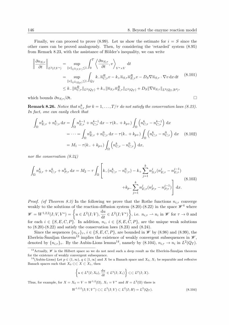
146 8. Beyond the enzyme reaction model
Finally, we can proceed to prove (8.99). Let us show the estimate for i = S since theother cases can be proved analogously. Then, by considering the ‘retarded’ system (8.95)from Remark 8.23, with the assistance of Holder’s inequality, we can write∥∥∥∥∂nS,τ∂t
∥∥∥∥L2(I;V ∗)
= sup‖v‖L2(I;V )≤1
ˆ T
0
⟨∂nS,τ∂t
, v
⟩V ∗×V
dt
= sup‖v‖L2(QT )≤1
ˆQT
k−nRC,τv − k+nS,τn
RE,τv −DS∇nS,τ · ∇v dx dt
≤ k−‖nRC,τ‖L2(QT ) + k+‖nS,τnRE,τ‖L2(QT ) +DS‖∇nS,τ‖L2(QT ,Rd),
(8.101)
which bounds ∂nS,τ/∂t.
Remark 8.26. Notice that nki,τ for k = 1, . . . , T/τ do not satisfy the conservation laws (8.23).In fact, one can easily check that
ˆΩnkE,τ + nkC,τ dx =
ˆΩnk−1E,τ + nk−1
C,τ dx− τ(k− + kp+)
ˆΩ
(nkC,τ − nk−1
C,τ
)dx
= · · · =ˆ
Ωn0E,τ + n0
C,τ dx− τ(k− + kp+)
ˆΩ
(nkC,τ − n0
C,τ
)dx
= M1 − τ(k− + kp+)
ˆΩ
(nkC,τ − n0
C,τ
)dx,
(8.102)
nor the conservation (8.24)
ˆΩnkS,τ + nkC,τ + nkP,τ dx = M2 − τ
ˆΩ
k−(nkC,τ − n0C,τ )− k+
k∑j=1
njS,τ (njE,τ − nj−1E,τ )
+kp−
k∑j=1
njE,τ (njP,τ − nj−1P,τ )
dx.
(8.103)
Proof. (of Theorem 8.3) In the following we prove that the Rothe functions ni,τ convergeweakly to the solutions of the reaction-diffusion system (8.20)-(8.22) in the space W 4 where
W = W 1,2,2(I;V, V ∗) =
u ∈ L2(I;V ),
du
dt∈ L2(I;V ∗)
, i.e. ni,τ ni in W for τ → 0 and
for each i ∈ S,E,C, P. In addition, ni, i ∈ S,E,C, P, are the unique weak solutionsto (8.20)-(8.22) and satisfy the conservation laws (8.23) and (8.24).
Since the sequences ni,ττ , i ∈ S,E,C, P, are bounded in W by (8.98) and (8.99), theEberlein-Smuljan theorem13 implies the existence of weakly convergent subsequences in W ,denoted by ni,ττ . By the Aubin-Lions lemma14, namely by (8.104), ni,τ → ni in L2(QT ).
13Actually, W is the Hilbert space so we do not need such a deep result as the Eberlein-Smuljan theoremfor the existence of weakly convergent subsequence.
14(Aubin-Lions) Let p ∈ (1,∞), q ∈ [1,∞] and X be a Banach space and X0, X1 be separable and reflexiveBanach spaces such that X0 ⊂⊂ X ⊂ X1, then
u ∈ Lp(I;X0),du
dt∈ Lq(I;X1)
⊂⊂ Lp(I;X).
Thus, for example, for X = X0 = V = W 1,2(Ω), X1 = V ∗ and H = L2(Ω) there is
W 1,2,2(I;V, V ∗) ⊂⊂ L2(I;V ) ⊂ L2(I;H) = L2(QT ). (8.104)
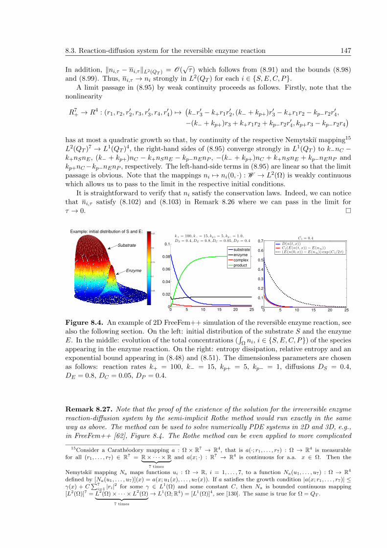
8.3. Reaction-diffusion system for the reversible enzyme reaction 147
In addition, ‖ni,τ − ni,τ‖L2(QT ) = O(√τ) which follows from (8.91) and the bounds (8.98)
and (8.99). Thus, ni,τ → ni strongly in L2(QT ) for each i ∈ S,E,C, P.A limit passage in (8.95) by weak continuity proceeds as follows. Firstly, note that the
nonlinearity
R7+ → R4 : (r1, r2, r
′2, r3, r
′3, r4, r
′4) 7→
(k−r
′3 − k+r1r
′2, (k− + kp+)r′3 − k+r1r2 − kp−r2r
′4,
−(k− + kp+)r3 + k+r1r2 + kp−r2r′4, kp+r3 − kp−r2r4
)has at most a quadratic growth so that, by continuity of the respective Nemytskiı mapping15
L2(QT )7 → L1(QT )4, the right-hand sides of (8.95) converge strongly in L1(QT ) to k−nC −k+nSnE , (k− + kp+)nC − k+nSnE − kp−nEnP , −(k− + kp+)nC + k+nSnE + kp−nEnP andkp+nC−kp−nEnP , respectively. The left-hand-side terms in (8.95) are linear so that the limitpassage is obvious. Note that the mappings ni 7→ ni(0, ·) : W → L2(Ω) is weakly continuouswhich allows us to pass to the limit in the respective initial conditions.
It is straightforward to verify that ni satisfy the conservation laws. Indeed, we can noticethat ni,τ satisfy (8.102) and (8.103) in Remark 8.26 where we can pass in the limit forτ → 0.
Example: initial distribution of S and E:
0.05
0.1
0.15
0.2
0.25
Substrate
Enzyme
0 5 10 15 20 250
0.02
0.04
0.06
0.08
0.1
k+ = 100, k−= 15, kp+ = 5, kp− = 1.0,
DS = 0.4, DE = 0.8, DC = 0.05, DP = 0.4
substrate
enzyme
complex
product
0 5 10 15 20 250
0.1
0.2
0.3
0.4
0.5
0.6
0.7C1 = 0.4
D(n(t, x))C1(E(n(t, x)) − E(n∞))(E(n(0, x)) − E(n∞)) exp (C1/2 t)
Figure 8.4. An example of 2D FreeFem++ simulation of the reversible enzyme reaction, seealso the following section. On the left: initial distribution of the substrate S and the enzymeE. In the middle: evolution of the total concentrations (
´Ω ni, i ∈ S,E,C, P) of the species
appearing in the enzyme reaction. On the right: entropy dissipation, relative entropy and anexponential bound appearing in (8.48) and (8.51). The dimensionless parameters are chosenas follows: reaction rates k+ = 100, k− = 15, kp+ = 5, kp− = 1, diffusions DS = 0.4,DE = 0.8, DC = 0.05, DP = 0.4.
Remark 8.27. Note that the proof of the existence of the solution for the irreversible enzymereaction-diffusion system by the semi-implicit Rothe method would run exactly in the sameway as above. The method can be used to solve numerically PDE systems in 2D and 3D, e.g.,in FreeFem++ [62], Figure 8.4. The Rothe method can be even applied to more complicated
15Consider a Caratheodory mapping a : Ω × R7 → R4, that is a(·; r1, . . . , r7) : Ω → R4 is measurablefor all (r1, . . . , r7) ∈ R7 = R× · · · × R︸ ︷︷ ︸
7 times
and a(x; ·) : R7 → R4 is continuous for a.a. x ∈ Ω. Then the
Nemytskiı mapping Na maps functions ui : Ω → R, i = 1, . . . , 7, to a function Na(u1, . . . , u7) : Ω → R4
defined by [Na(u1, . . . , u7)](x) = a(x;u1(x), . . . , u7(x)). If a satisfies the growth condition |a(x; r1, . . . , r7)| ≤γ(x) + C
∑7i=1 |ri|
2 for some γ ∈ L1(Ω) and some constant C, then Na is bounded continuous mapping[L2(Ω)]7 = L2(Ω)× · · · × L2(Ω)︸ ︷︷ ︸
7 times
→ L1(Ω;R4) = [L1(Ω)]4, see [130]. The same is true for Ω = QT .

148 8. Beyond the enzyme reaction model
systems such as the 2-compartmental reaction-diffusion systems for the p53 network studiedin Chapters 5 and 6.
FreeFem++ code for the reversible EnR system
Let us also print out the full FreeFem++ code for the reversible enzyme reaction, in particular,the implementation of the scheme (8.92). We hope that the code can be easily adapted to thep53 PDE models (the codes for the p53 models are lengthy, thus not shown here; however,they are available upon request). All the computed data are saved to text files which can bethen open by other software (e.g., by Matlab). In particular, the concentrations from eachtime step are saved to “info concentrations.txt”, the entropy, entropy dissipation and relativeentropy to “info entropy.txt” and information about the preserved conservation of masses in“info mass.txt”. The output from the code (with the given parameters and initial data) isshown on Fig. 8.4.
// —————————————————————————————————-//// Reversible Enzyme Reaction 2D RD model// by Jan Elias//// —————————————————————————————————-
load ”medit”load ”lapack”
// ——————————– constants & parameters ————————————
// technical constants ...string numb, numb2; int pos; // for a proper data savingreal[int] CameraPositionValue1 = [1.0851,2.77975,1.15398]; // for plotsreal[int] CameraFocalPointValue1 = [0,0,0.319209];real[int] CameraViewUpValue1 = [-0.0979641,-0.25096,0.963028];real[int] CameraClippingRangeValue1 = [1.4961,5.12329];real[int] CameraPositionValue = [1.95179,3.32595,2.50164];real[int] CameraFocalPointValue = [-0.0103131,-0.0187419,0.126953];real[int] CameraViewUpValue = [-0.254544,-0.456112,0.852742];real[int] CameraClippingRangeValue = [2.16186,7.62003];
// kinetic ratesreal kp1=100.0; // k +real km1=15.0; // k -real kp2=5.0; // k p+real km2=1.0; // k p-
// diffusionsreal Ds=0.4, De=0.8, Dc=0.005, Dp=0.4;
// time lag dt, final time T, frequency of saving datareal dt=0.02; real frq = 0.04; real T = 25.01;

8.3. Reaction-diffusion system for the reversible enzyme reaction 149
// constants appearing in the iteration process; num. precision is *tol*real tol=1e-6; int iter; int itermax=10;
real ctotal, etotal, stotal, ptotal; // total concentrationsreal cinit, einit, sinit, pinit; // initial concentrationsreal sigmas, sigmae, sigmac,sigmap; // σi dependent on the kinetic ratesreal ceq, eeq, seq, peq; // equilibriareal M1, M2, M1init, M2init; // masses from concervation lawsreal err, errM1, errM2; real [int] errM(2);real entrfun, entrdis, relentr; // entropy functional, entropy dissipation, relative entropy
// Macro for gradientmacro Grad(u) [dx(u),dy(u)] //
// 2D domain Ω, the disc of volume 1int In=1; // label of the border ∂Ωreal r = 1.0/sqrt(pi); // radiusborder C(t=0,2*pi) x=r*cos(t); y=r*sin(t); label=In;mesh Th=buildmesh(C(100));
// save and plot meshsavemesh (Th,”mesh.msh”);plot(Th,wait=1);
// space of functions on Thfespace Vh(Th,P1);
// indices: 0-S, 1-E, 2-C, 3-P// in the numerical scheme: ”uiold” are solutions from the old time step;// ”ui” are newly computed solutions at the current time step;// ”vi” are test functions;// ”uki” are refinements of ”ui” at each time step (so that the masses are conserved)Vh uk0,uk1,uk2,uk3, u0,u1,u2,u3, v0,v1,v2,v3;Vh u0old,u1old,u2old,u3old;
// initial conditionsfunc fs=0.4*( (x+0.3)ˆ2+(y+0.3)ˆ2<=0.25ˆ2 );func fe=2.5*( (x-0.4)ˆ2+yˆ2<0.05ˆ2 );func fc=0.0;func fp=0.0;
uk0=1e-15+fs; uk1=1e-15+fe; uk2=1e-10+fc; uk3=1e-10+fp;u0old=uk0; u1old=uk1; u2old=uk2; u3old=uk3;
// plot initial dataplot(uk0,value=1,fill=1,wait=1,dim=3,ColorScheme=1,ShowAxes=0);plot(uk1,value=1,fill=1,wait=1,dim=3,ColorScheme=1,ShowAxes=0);plot(uk2,value=1,fill=1,wait=1,dim=3,ColorScheme=1,ShowAxes=0);plot(uk3,value=1,fill=1,wait=1,dim=3,ColorScheme=1,ShowAxes=0);

150 8. Beyond the enzyme reaction model
// total mass, conservation lawssinit=int2d(Th)(uk0); einit=int2d(Th)(uk1); //Lˆ1 normcinit=int2d(Th)(uk2); pinit=int2d(Th)(uk3); //Lˆ1 norm
M1init=cinit+einit; M2init=sinit+cinit+pinit;
// save information about the conservation of masses into the text file ”info mass.txt”ofstream ff(”info mass.txt”);ff << ”time = 0.0, M1 (M1init) = ” << M1init << ” (” << M1init << ”),
M2 (M2init) = ” << M2init << ” (” << M2init << ”)” <<endl;
// equilibria (computed analytically): ceq, eeq, seq, peqreal alpha=1.0, beta=km1/kp2;sigmas=kp1/km1; sigmae=alpha*km1; sigmac=alpha*km1; sigmap=km2/kp2;real capitalK = ((sigmas+sigmap)*sigmac)/(sigmas*sigmae*sigmap);
ceq = (M1init+M2init+capitalK - sqrt( (M1init+M2init+capitalK)ˆ2 -4*M1init*M2init) )/2;eeq = M1init - ceq;seq = (km1*ceq)/(kp1*eeq);peq = (kp2*ceq)/(km2*eeq);
// entropyentrfun=int2d(Th)( uk0*log(sigmas*uk0)-uk0+1.0/sigmas + uk1*log(sigmae*uk1)-uk1+1.0/sigmae
+ uk2*log(sigmac*uk2)-uk2+1.0/sigmac + uk3*log(sigmap*uk3)-uk3+1.0/sigmap );
// entropy dissipationentrdis=int2d(Th)( Ds*(Grad(uk0)’*Grad(uk0))/uk0
+ De*(Grad(uk1)’*Grad(uk1))/uk1+ Dc*(Grad(uk2)’*Grad(uk2))/uk2+ Dp*(Grad(uk3)’*Grad(uk3))/uk3 )
+ int2d(Th)( (kp1*uk0*uk1-km1*uk2)*(log(sigmas*sigmae*uk0*uk1)-log(sigmac*uk2)) )+ int2d(Th)( (km2*uk1*uk3-kp2*uk2)*(log(sigmae*sigmap*uk1*uk3)-log(sigmac*uk2)) );
// relative entropyrelentr=int2d(Th)( uk0*log(uk0/seq)-(uk0-seq) + uk1*log(uk1/eeq)-(uk1-eeq)
+ uk2*log(uk2/ceq)-(uk2-ceq) + uk3*log(uk3/peq)-(uk3-peq) );
// save concentrations into the text file ”info concentrations.txt”ofstream hh(”info concentrations.txt”);hh << ”0,” << sinit << ”,” << seq << ”,” << einit << ”,” << eeq << ”,”
<< cinit << ”,” << ceq << ”,” << pinit << ”,” << peq << endl;
// save concentrations into the text file ”info entropy.txt”ofstream en(”info entropy.txt”);en << ”0” << ”,” << entrfun << ”,” << entrdis << ”,” << relentr << endl;
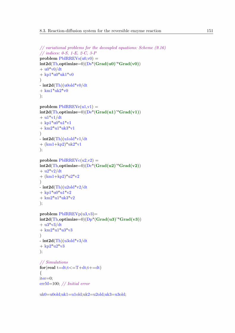
8.3. Reaction-diffusion system for the reversible enzyme reaction 151
// variational problems for the decoupled equations: Scheme (9.16)// indices: 0-S, 1-E, 2-C, 3-Pproblem PbIRREVs(u0,v0) =int2d(Th,optimize=0)(Ds*(Grad(u0)’*Grad(v0))+ u0*v0/dt+ kp1*u0*uk1*v0)- int2d(Th)(u0old*v0/dt+ km1*uk2*v0);
problem PbIRREVe(u1,v1) =int2d(Th,optimize=0)(De*(Grad(u1)’*Grad(v1))+ u1*v1/dt+ kp1*u0*u1*v1+ km2*u1*uk3*v1)- int2d(Th)(u1old*v1/dt+ (km1+kp2)*uk2*v1);
problem PbIRREVc(u2,v2) =int2d(Th,optimize=0)(Dc*(Grad(u2)’*Grad(v2))+ u2*v2/dt+ (km1+kp2)*u2*v2)- int2d(Th)(u2old*v2/dt+ kp1*u0*u1*v2+ km2*u1*uk3*v2);
problem PbIRREVp(u3,v3)=int2d(Th,optimize=0)(Dp*(Grad(u3)’*Grad(v3))+ u3*v3/dt+ km2*u1*u3*v3)- int2d(Th)(u3old*v3/dt+ kp2*u2*v3);
// Simulationsfor(real t=dt;t<=T+dt;t+=dt)iter=0;errM=100; // Initial error
uk0=u0old;uk1=u1old;uk2=u2old;uk3=u3old;

152 8. Beyond the enzyme reaction model
while(errM.max¿tol && iter<itermax) // refinement to reach conservation of masses M1 and M2
// Solving variational problemsPbIRREVs;PbIRREVe;PbIRREVc;PbIRREVp;
iter++;
stotal=int2d(Th)(u0); etotal=int2d(Th)(u1); //Lˆ1 normctotal=int2d(Th)(u2); ptotal=int2d(Th)(u3);M1=ctotal+etotal; M2=stotal+ctotal+ptotal;
errM1=abs(M1init-M1); errM2=abs(M2init-M2);errM[0]=errM1; errM[1]=errM2;
uk0=u0; uk1=u1; uk2=u2; uk3=u3; // new refinements
// eof while
if ((iter==itermax) && (errM.min¿tol*10))
cout << ”Max. number of allowed iterations reached!” << endl;break;
// save, print desired data (results) after each ”frq” iterationnumb = string(t/frq); pos = numb.find(”.”); numb2 = numb(pos+1:numb.length);if ( pos == -1 ? 1 : (numb2==”0” ? 1 : 0)) // save/plot data
numb = string(t);pos = numb.find(”.”);numb2 = numb(0:pos+2);
plot(Th,u0,u3,wait=0,value=1,fill=1,dim=3,aspectratio=1,ZScale=0.5,ColorScheme=1,ShowAxes=0,nbiso=160,NbColorTicks=6,LabelColors=2,CameraPosition = CameraPositionValue1,CameraFocalPoint = CameraFocalPoint-Value1,CameraViewUp = CameraViewUpValue1,CameraViewAngle = 30, CameraClippingRange = CameraClippingRangeValue1,cmm=t);
stotal=int2d(Th)(u0); etotal=int2d(Th)(u1); //Lˆ1 normctotal=int2d(Th)(u2); ptotal=int2d(Th)(u3);M1=ctotal+etotal; M2=stotal+ctotal+ptotal;

8.3. Reaction-diffusion system for the reversible enzyme reaction 153
hh << t << ”,” << stotal << ”,” << seq << ”,” << etotal << ”,” << eeq << ”,” << cto-tal << ”,” << ceq
<< ”,” << ptotal << ”,” << peq << endl;ff << ”time = ” << t << ”; M1 (M1init) = ” << M1 << ” (” << M1init <<
”), M2 (M2init) = ” << M2<< ” (” << M2init << ”)” <<endl;
entrfun=int2d(Th)( u0*log(sigmas*u0)-u0+1.0/sigmas + u1*log(sigmae*u1)-u1+1.0/sigmae
+ u2*log(sigmac*u2)-u2+1.0/sigmac + u3*log(sigmap*u3)-u3+1.0/sigmap );entrdis=int2d(Th)( Ds*(Grad(u0)’*Grad(u0))/u0 + De*(Grad(u1)’*Grad(u1))/u1
+ Dc*(Grad(u2)’*Grad(u2))/u2 + Dp*(Grad(u3)’*Grad(u3))/u3)+ int2d(Th)( (kp1*u0*u1-km1*u2)*(log(sigmas*sigmae*u0*u1)-log(sigmac*u2)) )+ int2d(Th)( (km2*u1*u3-kp2*u2)*(log(sigmae*sigmap*u1*u3)-log(sigmac*u2)) );
relentr=int2d(Th)( u0*log(u0/seq)-(u0-seq) + u1*log(u1/eeq)-(u1-eeq)+ u2*log(u2/ceq)-(u2-ceq) + u3*log(u3/peq)-(u3-peq) );
en << t << ”,” << entrfun << ”,” << entrdis << ”,” << relentr << endl;
// save current solution for the next time stepu0old=u0;u1old=u1;u2old=u2;u3old=u3;// ————————————————–

154 8. Beyond the enzyme reaction model

Bibliography
[1] B. Alberts, A. Johnson, J. Lewis, M. Raff, K. Roberts, and P. Walter. Molecular Biologyof the Cell. Garland Science. Taylor and Francis Group, fifth edition, 2008.
[2] U. Alon. http://wws.weizmann.ac.il/mcb/UriAlon/.
[3] A. Arnold, J. A. Carrillo, L. Desvillettes, J. Dolbeault, A. Jungel, C. Lederman, P. A.Markowich, G. Toscani, and C. Villani. Entropies and equilibria of many-particle sys-tems: An essay on recent research. Monatshefte fur Mathematik, 142(1-2):35–43, 2004.
[4] B. D. Aronson, K. A. Johnson, and J. C. Dunlap. Circadian clock locus frequency:protein encoded by a single open reading frame defines period length and temperaturecompensation. Proc. Nat. Acad. Sci. USA, 91(16):7683–7687, 1994.
[5] M. Ashcroft, R. L. Ludwig, D. B. Woods, T. D. Copeland, H. O. Weber, E. J. MacRae,and K. H. Vousden. Phosphorylation of HDM2 by Akt. Oncogene, 21(13):1955–1962,2002.
[6] T. J. Atkinson and M. S. Halfon. Regulation of gene expression in the genomic context.Computational and structural biotechnology journal, 9(13):e201401001, 2014.
[7] C. J. Bakkenist and M. B. Kastan. DNA damage activates ATM through intermolecularautophosphorylation and dimer dissociation through intermolecular autophosphoryla-tion and dimer dissociation. Nature, 421(6922):499–506, 01 2003.
[8] A. Ballesta, J. Clairambault, S. Dulong, and F. Levi. A systems biomedicine ap-proach for chronotherapeutics optimization: Focus on the anticancer drug irinotecan.In A. d’Onofrio, P. Cerrai, and A. Gandolfi, editors, New Challenges for Cancer SystemsBiomedicine, SIMAI Springer Series, pages 301–327. Springer Milan, 2012.
[9] A. Ballesta, S. Dulong, C. Abbara, B. Cohen, A. Okyar, J. Clairambault, and F. Levi.A combined experimental and mathematical approach for molecular-based optimizationof irinotecan circadian delivery. PLoS Comput Biol, 7(9):e1002143, 09 2011.
[10] Y. Barak, E. Gottlieb, T. Juven-Gershon, and M. Oren. Regulation of mdm2 expres-sion by p53: alternative promoters produce transcripts with nonidentical translationpotential. Genes & Development, 8(15):1739–1749, 1994.
[11] Y. Barak, T. Juven, R. Haffner, and M. Oren. mdm2 expression is induced by wildtype p53 activity. The EMBO Journal, 12(2):461–468, 02 1993.
[12] J. A. Barboza, T. Iwakuma, T. Terzian, A. K. El-Naggar, and G. Lozano. Mdm2 andmdm4 loss regulates distinct p53 activities. Molecular Cancer Research, 6(6):947–954,2008.
155

156 BIBLIOGRAPHY
[13] J. Bartkova, C. J. Bakkenist, E. R.-D. Meyts, N. E. Skakkebæk, M. Sehested, J. Lukas,M. B. Kastan, and J. Bartek. ATM activation in normal human tissues and testicularcancer. Cell Cycle, 4(6):838–845, 2005.
[14] E. Batchelor, A. Loewer, C. Mock, and G. Lahav. Stimulus-dependent dynamics of p53in single cells. Molecular Systems Biology, 7(1):8 pp, 2011.
[15] E. Batchelor, C. S. Mock, I. Bhan, A. Loewer, and G. Lahav. Recurrent initiation:A mechanism for triggering p53 pulses in response to DNA damage. Molecular Cell,30(3):277–289, 2015/02/16 2008.
[16] S. Ben-Tabou de Leon and E. H. Davidson. Modeling the dynamics of transcriptionalgene regulatory networks for animal development. Developmental biology, 325(2):317–328, 2009.
[17] M. Bendahmane, T. Lepoutre, A. Marrocco, and B. Perthame. Conservative crossdiffusions and pattern formation through relaxation. Journal de Mathematiques Pureset Appliquees, 92(6):651–667, 2009.
[18] E. Berkovich, R. J. Monnat, and M. B. Kastan. Roles of ATM and NBS1 in chro-matin structure modulation and DNA double-strand break repair. Nature Cell Biology,9(6):683–690, 06 2007.
[19] F. Billy and J. Clairambault. Designing proliferating cell population models with func-tional targets for control by anti-cancer drugs. Discrete and Continuous DynamicalSystems - Series B, 18(4):865–889, 2013.
[20] J. Braga, J. G. McNally, and M. Carmo-Fonseca. A reaction-diffusion model to studyRNA motion by quantitative fluorescence recovery after photobleaching. BiophysicalJournal, 92(8):2694–2703, 2007.
[21] G. E. Briggs and J. B. S. Haldane. A note on the kinetics of enzyme action. BiochemicalJournal, 19:338–339, 1925.
[22] N. F. Britton. Reaction-diffusion equations and their applications to biology. AcademicPress, London, 1986.
[23] A. Cangiani and R. Natalini. A spatial model of cellular molecular trafficking includingactive transport along microtubules. Journal of theoretical biology, 267(4):614–625,2010.
[24] L. C. Cantley and B. G. Neel. New insights into tumor suppression: PTEN suppressestumor formation by restraining the phosphoinositide 3-kinase/AKT pathway. Proc.Natl. Acad. Sci. USA, 96(8):4240–4245, 1999.
[25] C.-J. Chang, D. J. Freeman, and H. Wu. PTEN regulates Mdm2 expression throughthe P1 promoter. Journal of Biological Chemistry, 279(28):29841–29848, 2004.
[26] Y. Chang, Y. Lee, T. Tejima, K. Tanaka, S. Omura, N. Heintz, Y. Mitsui, and J. Ma-gae. mdm2 and bax, downstream mediators of the p53 response, are degraded by theubiquitin-proteasome pathway. Cell Growth Differ, 9(1):79–84, 1998.
[27] C. Y. Chen, J. D. Oliner, Q. Zhan, A. J. Fornace, B. Vogelstein, and M. B. Kas-tan. Interactions between p53 and MDM2 in a mammalian cell cycle checkpoint path-way. Proceedings of the National Academy of Sciences of the United States of America,91(7):2684–2688, 03 1994.

BIBLIOGRAPHY 157
[28] A. Ciliberto, B. Novak, and J. J. Tyson. Steady states and oscillations in the p53/Mdm2network. Cell cycle, 4(3):488–493, 2005.
[29] J. Clairambault. Modelling physiological and pharmacological control on cell prolifer-ation to optimise cancer treatments. Mathematical Modelling of Natural Phenomena,4:12–67, 1 2009.
[30] J. Clairambault and O. Fercoq. Physiologically structured cell population dynamicmodels with applications to combined drug delivery optimisation in oncology. InM. Bachar, J. Batzel, and M. Chaplain, editors, Mathematical modelling of cancergrowth and treatment. Springer, 2013.
[31] D. Claude and J. Clairambault. Period shift induction by intermittent stimulation in aDrosophila model of per protein oscillations. Chronobiology international, 17(1):1–14,2000.
[32] C. N. Cole and J. J. Scarcelli. Transport of messenger RNA from the nucleus to thecytoplasm. Current opinion in cell biology, 18(3):299–306, 2006.
[33] T. Deerinck and M. Ellisman. Photograph : Death most beautiful (2008) taken fromhttp://www.cell.com/cell picture show-celldeath.
[34] C. DeFranco, M. E. Chicurel, and H. Potter. A general RNA-binding protein complexthat includes the cytoskeleton-associated protein MAP 1A. Molecular biology of thecell, 9(7):1695–1708, 1998.
[35] D. L. Denault, J. J. Loros, and J. C. Dunlap. WC-2 mediates WC-1–FRQ interactionwithin the PAS protein-linked circadian feedback loop of Neurospora. The EMBOjournal, 20(1-2):109–117, 2001.
[36] N. Desilet, T. N. Campbell, and F. Y. Choy. p53-based anti-cancer therapies: an emptypromise? Current issues in molecular biology, 12(3):143, 2010.
[37] L. Desvillettes and K. Fellner. Exponential decay toward equilibrium via entropy meth-ods for reaction–diffusion equations. Journal of Mathematical Analysis and Applica-tions, 319(1):157–176, 2006.
[38] L. Desvillettes and K. Fellner. Duality- and entropy methods for reversible reaction-diffusion equations with degenerate diffusion. Preprint, 2014.
[39] L. Desvillettes and K. Fellner. Exponential convergence to equilibrium for a nonlinearreaction-diffusion systems arising in reversible chemistry. In C. Potzsche, C. Heuberger,B. Kaltenbacher, and F. Rendl, editors, System Modeling and Optimization, volume443 of IFIP Advances in Information and Communication Technology, pages 96–104.Springer Berlin Heidelberg, 2014.
[40] L. Desvillettes, K. Fellner, M. Pierre, and J. Vovelle. About global existence forquadratic systems of reaction-diffusion. Journal Advanced Nonlinear Studies, 7:491–511, 2007.
[41] A. Dhooge, W. Govaerts, and Y. A. Kuznetsov. MATCONT: a MATLAB package fornumerical bifurcation analysis of ODEs. ACM Transactions on Mathematical Software(TOMS), 29(2):141–164, 2003.

158 BIBLIOGRAPHY
[42] L. Dimitrio. Modelling nucleocytoplasmic transport with application to the intracellulardynamics of the tumor suppressor protein p53. PhD thesis, Universite Pierre et MarieCurie, Paris, September 2012.
[43] L. Dimitrio, J. Clairambault, and R. Natalini. A spatial physiological model for p53intracellular dynamics. Journal of Theoretical Biology, 316(0):9–24, 2013.
[44] J. C. Dunlap. Molecular bases for circadian clocks. Cell, 96(2):271–290, 1999.
[45] J. Elias and J. Clairambault. Reaction–diffusion systems for spatio-temporal intra-cellular protein networks: A beginner’s guide with two examples. Computational andStructural Biotechnology Journal, 10(16):12–22, 2014.
[46] J. Elias, L. Dimitrio, J. Clairambault, and R. Natalini. The dynamics of p53 in singlecells: physiologically based ODE and reaction–diffusion PDE models. Physical Biology,11(4):045001, 2014.
[47] J. Elias, L. Dimitrio, J. Clairambault, and R. Natalini. The p53 protein and its molec-ular network: Modelling a missing link between DNA damage and cell fate. Biochimicaet Biophysica Acta (BBA) - Proteins and Proteomics, 1844(1, Part B):232–247, 2014.
[48] L. C. Evans. Partial Differential Equations. Graduate Studies in Mathematics, V. 19.AMS, Providence, second edition, 2010.
[49] S. S. Fakharzadeh, S. P. Trusko, and D. L. George. Tumorigenic potential associatedwith enhanced expression of a gene that is amplified in a mouse tumor cell line. TheEMBO Journal, 10(6):1565–1569, 06 1991.
[50] J. Falck, J. Coates, and S. P. Jackson. Conserved modes of recruitment of ATM, ATRand DNA-PKcs to sites of DNA damage. Nature, 434(7033):605–611, 03 2005.
[51] K. Fellner. Reaction-diffusion equations. Lecture notes, 2010.
[52] M. Fiscella, H. Zhang, S. Fan, K. Sakaguchi, S. Shen, W. E. Mercer, G. F. Vande Woude,P. M. O’Connor, and E. Appella. Wip1, a novel human protein phosphatase that isinduced in response to ionizing radiation in a p53-dependentmanner. Proceedings of theNational Academy of Sciences, 94(12):6048–6053, 1997.
[53] P. N. Friedman, X. Chen, J. Bargonetti, and C. Prives. The p53 protein is an unusuallyshaped tetramer that binds directly to DNA. Proc. Natl. Acad. Sci. USA, 90(8):3319–3323, 1993.
[54] M. Gajjar, M. M. Candeias, L. Malbert-Colas, A. Mazars, J. Fujita, V. Olivares-Illana,and R. Fahraeus. The p53 mRNA-Mdm2 interaction controls Mdm2 nuclear traffickingand is required for p53 activation following DNA damage. Cancer Cell, 21(1):25–35,2012.
[55] N. Y. Garceau, Y. Liu, J. J. Loros, and J. C. Dunlap. Alternative initiation of transla-tion and time-specific phosphorylation yield multiple forms of the essential clock proteinFREQUENCY. Cell, 89(3):469–476, 1997.
[56] N. Geva-Zatorsky, N. Rosenfeld, S. Itzkovitz, R. Milo, A. Sigal, E. Dekel, T. Yarnitzky,Y. Liron, P. Polak, G. Lahav, and U. Alon. Oscillations and variability in the p53system. Molecular Systems Biology, 2(1):1–13, 2006.
BIBLIOGRAPHY 159
[57] B. C. Goodwin. Oscillatory behavior in enzymatic control processes. Advances inenzyme regulation, 3:425–438, 1965.
[58] T. M. Gottlieb, J. Leal, R. Seger, Y. Taya, and M. Oren. Cross-talk between Akt, p53and Mdm2: possible implications for the regulation of apoptosis. Oncogene, 21(8):1299–1303, 2002.
[59] D. R. Green and G. Kroemer. Cytoplasmic functions of the tumour suppressor p53.Nature, 458(7242):1127–1130, 04 2009.
[60] S. L. Harris and A. J. Levine. The p53 pathway: positive and negative feedback loops.Oncogene, 24(17):2899–2908, 2005.
[61] Y. Haupt, R. Maya, A. Kazaz, and M. Oren. Mdm2 promotes the rapid degradationof p53. Nature, 387(6630):296–299, 05 1997.
[62] F. Hecht. New development in FreeFem++. Journal of Numerical Mathematics, 20(3-4):251–265, 2012.
[63] F. G. Heineken, H. M. Tsuchiya, and R. Aris. On the mathematical status of the pseudo-steady state hypothesis of biochemical kinetics. Mathematical Biosciences, 1(1):95–113,1967.
[64] P. Hinow, C. E. Rogers, C. E. Barbieri, J. A. Pietenpol, A. K. Kenworthy, andE. DiBenedetto. The DNA binding activity of p53 displays reaction-diffusion kinet-ics. Biophysical journal, 91(1):330–342, 2006.
[65] S. Hong, Y.-N. Wang, H. Yamaguchi, H. Sreenivasappa, C.-K. Chou, P.-H. Tsou, M.-C. Hung, and J. Kameoka. Measurement of protein 53 diffusion coefficient in live helacells using raster image correlation spectroscopy (rics). Journal of biomaterials andnanobiotechnology, 1(1):31–36, 2010.
[66] A. C. Joerger and A. R. Fersht. The tumor suppressor p53: from structures to drugdiscovery. Cold Spring Harbor Perspectives in Biology, 2(6):a000919, 2010.
[67] M. B. Kastan and J. Bartek. Cell-cycle checkpoints and cancer. Nature, 432(7015):316–323, 11 2004.
[68] J. Keener and J. Sneyd. Mathematical Physiology I: Cellular Physiology. Interdisci-plinary Applied Mathematics. Springer, second edition, 2009.
[69] J. K. Kim and T. L. Jackson. Mechanisms that enhance sustainability of p53 pulses.PloS, 8(6):e65242, 2013.
[70] R. Kitagawa, C. J. Bakkenist, P. J. McKinnon, and M. B. Kastan. Phosphorylation ofSMC1 is a critical downstream event in the ATM–NBS1–BRCA1 pathway. Genes &Development, 18(12):1423–1438, 2004.
[71] S. V. Kozlov, M. E. Graham, B. Jakob, F. Tobias, A. W. Kijas, M. Tanuji, P. Chen,P. J. Robinson, G. Taucher-Scholz, K. Suzuki, S. So, D. Chen, and M. F. Lavin. Au-tophosphorylation and ATM activation: additional sites add to the complexity. Journalof Biological Chemistry, 286(11):9107–9119, 2011.
[72] S. V. Kozlov, M. E. Graham, C. Peng, P. Chen, P. J. Robinson, and M. F. a. Lavin.Involvement of novel autophosphorylation sites in ATM activation. The EMBO Journal,25(15):3504–3514, 07 2006.

160 BIBLIOGRAPHY
[73] M. Kracikova, G. Akiri, A. George, R. Sachidanandam, and S. A. Aaronson. A thresholdmechanism mediates p53 cell fate decision between growth arrest and apoptosis. CellDeath Differ, 20(4):576–588, 04 2013.
[74] M. H. G. Kubbutat, S. N. Jones, and K. H. Vousden. Regulation of p53 stability byMdm2. Nature, 387(6630):299–303, 05 1997.
[75] Y. A. Kuznetsov. Elements of applied bifurcation theory. Springer-Verlag, New York,third edition, 2004.
[76] O. A. Ladyzhenskaya, V. A. Solonnikov, and N. N. Uraltseva. Linear and quasi-linearequations of parabolic type, volume 23. American Mathematical Soc., 1968.
[77] G. Lahav, N. Rosenfeld, A. Sigal, N. Geva-Zatorsky, A. J. Levine, M. B. Elowitz, andU. Alon. Dynamics of the p53-Mdm2 feedback loop in individual cells. Nat Genet,36(2):147–150, 02 2004.
[78] Z. Lai, K. V. Ferry, M. A. Diamond, K. E. Wee, Y. B. Kim, J. Ma, T. Yang, P. A.Benfield, R. A. Copeland, and K. R. Auger. Human mdm2 mediates multiple mono-ubiquitination of p53 by a mechanism requiring enzyme isomerization. Journal ofBiological Chemistry, 276(33):31357–31367, 2001.
[79] S. Lain and D. Lane. Improving cancer therapy by non-genotoxic activation of p53.European Journal of Cancer, 39(8):1053–1060, 2003.
[80] J. E. Landers, S. L. Cassel, and D. L. George. Translational enhancement of mdm2oncogene expression in human tumor cells containing a stabilized wild-type p53 protein.Cancer Research, 57(16):3562–3568, 1997.
[81] M. F. Lavin. Ataxia-telangiectasia: from a rare disorder to a paradigm for cell signallingand cancer. Nat Rev Mol Cell Biol, 9(12):759–769, 12 2008.
[82] J.-H. Lee and T. T. Paull. ATM activation by DNA double-strand breaks through theMre11-Rad50-Nbs1 complex. Science, 308(5721):551–554, 2005.
[83] Y. Lee, M. J. Chong, and P. J. McKinnon. Ataxia telangiectasia mutated-dependentapoptosis after genotoxic stress in the developing nervous system is determined bycellular differentiation status. The Journal of Neuroscience, 21(17):6687–6693, 2001.
[84] J.-C. Leloup and A. Goldbeter. A model for circadian rhythms in Drosophila incor-porating the formation of a complex between the PER and TIM proteins. Journal ofbiological rhythms, 13(1):70–87, 1998.
[85] J.-C. Leloup, D. Gonze, and A. Goldbeter. Limit cycle models for circadian rhythmsbased on transcriptional regulation in Drosophila and Neurospora. Journal of BiologicalRhythms, 14(6):433–448, 1999.
[86] R. Lev Bar-Or, R. Maya, L. A. Segel, U. Alon, A. J. Levine, and M. Oren. Generationof oscillations by the p53-Mdm2 feedback loop: A theoretical and experimental study.Proceedings of the National Academy of Sciences, 97(21):11250–11255, 10 2000.
[87] F. Levi, A. Okyar, S. Dulong, P. F. Innominato, and J. Clairambault. Circadian timingin cancer treatments. Annual Review of Pharmacology and Toxicology, 50(1):377–421,2010. PMID: 20055686.

BIBLIOGRAPHY 161
[88] A. J. Levine. The paths to death and differentiation. Cell Death & Differentiation,18(9):1391–1392, 2011.
[89] M. Li, C. L. Brooks, F. Wu-Baer, D. Chen, R. Baer, and W. Gu. Mono-versus polyu-biquitination: differential control of p53 fate by Mdm2. Science, 302(5652):1972–1975,2003.
[90] D. C. Link, L. G. Schuettpelz, D. Shen, J. Wang, M. J. Walter, S. Kulkarni, J. E.Payton, J. Ivanovich, P. J. Goodfellow, M. Le Beau, et al. Identification of a novelTP53 cancer susceptibility mutation through whole-genome sequencing of a patientwith therapy-related AML. Jama, 305(15):1568–1576, 2011.
[91] A. Loewer, K. Karanam, C. Mock, and G. Lahav. The p53 response in single cells islinearly correlated to the number of DNA breaks without a distinct threshold. BMCbiology, 11(114):13, 2013.
[92] X. Lu, T.-A. Nguyen, S.-H. Moon, Y. Darlington, M. Sommer, and L. A. Donehower.The type 2C phosphatase Wip1: An oncogenic regulator of tumor suppressor and DNAdamage response pathways. Cancer Metastasis Reviews, 27(2):123–135, 2008.
[93] C. Luo, J. J. Loros, and J. C. Dunlap. Nuclear localization is required for function ofthe essential clock protein FRQ. The EMBO Journal, 17(5):1228–1235, 1998.
[94] L. Ma, J. Wagner, J. J. Rice, W. Hu, A. J. Levine, and G. A. Stolovitzky. A plausiblemodel for the digital response of p53 to DNA damage. Proc. Natl. Acad. Sci. USA,102(40):14266–14271, 2005.
[95] L. Macurek, A. Lindqvist, O. Voets, J. Kool, H. R. Vos, and R. H. Medema. Wip1phosphatase is associated with chromatin and dephosphorylates γH2AX to promotecheckpoint inhibition. Oncogene, 29(15):2281–2291, 2010.
[96] L. Malbert-Colas, A. Ponnuswamy, V. Olivares-Illana, A.-S. Tournillon, N. Naski, andR. Fahraeus. HDMX folds the nascent p53 mRNA following activation by the ATMkinase. Molecular Cell, 54(3):500–511, 2014.
[97] N. Marchenko, W. Hanel, D. Li, K. Becker, N. Reich, and U. Moll. Stress-mediatednuclear stabilization of p53 is regulated by ubiquitination and importin-α3 binding.Cell Death & Differentiation, 17(2):255–267, 2010.
[98] R. Maya, M. Balass, S.-T. Kim, D. Shkedy, J.-F. M. Leal, O. Shifman, M. Moas,T. Buschmann, Z. Ronai, Y. Shiloh, M. B. Kastan, E. Katzir, and M. Oren. ATM-dependent phosphorylation of Mdm2 on serine 395: role in p53 activation by DNAdamage. Genes & Development, 15(9):1067–1077, 2001.
[99] L. D. Mayo, J. E. Dixon, D. L. Durden, N. K. Tonks, and D. B. Donner. PTEN protectsp53 from Mdm2 and sensitizes cancer cells to chemotherapy. Journal of BiologicalChemistry, 277(7):5484–5489, 2002.
[100] L. D. Mayo and D. B. Donner. A phosphatidylinositol 3-kinase/Akt pathway promotestranslocation of Mdm2 from the cytoplasm to the nucleus. Proceedings of the NationalAcademy of Sciences, 98(20):11598–11603, 2001.
[101] L. D. Mayo and D. B. Donner. The PTEN, Mdm2, p53 tumor suppressor–oncoproteinnetwork. Trends in Biochemical Sciences, 27(9):462–467, 2001.

162 BIBLIOGRAPHY
[102] D. W. Meek. The p53 response to DNA damage. DNA Repair, 3(8–9):1049–1056, 2004.
[103] D. W. Meek and U. Knippschild. Posttranslational modification of MDM2. MolecularCancer Research, 1(14):1017–1026, 12 2003.
[104] B. D. Melanson, R. Bose, J. D. Hamill, K. A. Marcellus, E. F. Pan, and B. C. McKay.The role of mRNA decay in p53-induced gene expression. RNA, 17(12):2222–2234,2011.
[105] D. Metzler. Biochemistry: the chemical reactions of living cells, volume 2. Elsevier,2003.
[106] D. Michael and M. Oren. The p53–Mdm2 module and the ubiquitin system. Seminarsin Cancer Biology, 13(1):49–58, 2003.
[107] L. Michaelis and M. Menten. Die kinetik der invertinwirkung. Biochem. Z., 49:333–369,1913.
[108] R. Mirzayans, B. Andrais, A. Scott, and D. Murray. New insights into p53 signaling andcancer cell response to dna damage: implications for cancer therapy. BioMed ResearchInternational, 2012:16 pp, 2012.
[109] J. Momand, G. P. Zambetti, D. C. Olson, D. George, and A. J. Levine. The mdm-2oncogene product forms a complex with the p53 protein and inhibits p53-mediatedtransactivation. Cell, 69(7):1237–1245, 1992.
[110] J. D. Murray. Mathematical Biology II: Spatial Models and Biomedical Applications,volume 17 of Interdisciplinary Applied Mathematics. Springer, New York, third edition,2003.
[111] F. Murray-Zmijewski, E. A. Slee, and X. Lu. A complex barcode underlies the hetero-geneous response of p53 to stress. Nat Rev Mol Cell Biol, 9(9):702–712, 09 2008.
[112] E. Nagy. Basic equations of the mass transport through a membrane layer. Elsevier,first edition, 2012.
[113] Y. Ogawara, S. Kishishita, T. Obata, Y. Isazawa, T. Suzuki, K. Tanaka, N. Masuyama,and Y. Gotoh. Akt enhances Mdm2-mediated ubiquitination and degradation of p53.Journal of Biological Chemistry, 277(24):21843–21850, 2002.
[114] J. D. Oliner, K. W. Kinzler, P. S. Meltzer, D. L. George, and B. Vogelstein. Am-plification of a gene encoding a p53-associated protein in human sarcomas. Nature,358(6381):80–83, 07 1992.
[115] J. D. Oliner, J. A. Pietenpol, S. Thiagalingam, J. Gyuris, K. W. Kinzler, and B. Vogel-stein. Oncoprotein MDM2 conceals the activation domain of tumour suppressor p53.Nature, 362(6423):857–860, 04 1993.
[116] D. C. Olson, V. Marechal, J. Momand, J. Chen, C. Romocki, and A. Levine. Identifi-cation and characterization of multiple mdm-2 proteins and mdm-2-p53 protein com-plexes. Oncogene, 8(9):2353–2360, 1993.
[117] T. T. Paull and J.-H. Lee. The Mre11/Rad50/Nbs1 complex and its role as a DNAdouble-strand break sensor for ATM. Cell Cycle, 4(6):737–740, 2005.

BIBLIOGRAPHY 163
[118] Y. Peng, L. Chen, C. Li, W. Lu, S. Agrawal, and J. Chen. Stabilization of the MDM2oncoprotein by mutant p53. Journal of Biological Chemistry, 276(9):6874–6878, 2001.
[119] B. Perthame. Growth, reaction, movement and diffusion from biology. Lecture notes,2012.
[120] M. Pierre. Weak solutions and supersolutions in L1 for reaction-diffusion systems.In W. Arendt, H. Brezis, and M. Pierre, editors, Nonlinear Evolution Equations andRelated Topics, pages 153–168. Birkhauser Basel, 2004.
[121] M. Pierre. Global existence in reaction-diffusion systems with control of mass: a survey.Milan Journal of Mathematics, 78(2):417–455, 2010.
[122] M. Pierre and D. Schmitt. Blow-up in reaction diffusion systems with dissipation ofmass. Journal on Mathematical Analysis, 28(2):259–269, 1997.
[123] J. E. Purvis, K. W. Karhohs, C. Mock, E. Batchelor, A. Loewer, and G. Lahav. p53dynamics control cell fate. Science, 336(6087):1440–1444, 2012.
[124] J. E. Purvis and G. Lahav. Encoding and decoding cellular information through sig-naling dynamics. Cell, 152(5):945–956, 2013.
[125] K. Puszynski, A. Gandolfi, and A. d’Onofrio. The pharmacodynamics of the p53-Mdm2 targeting drug Nutlin: The role of gene-switching noise. PLoS Comput Biol,10(12):e1003991 EP, 2014.
[126] K. Puszynski, B. Hat, and T. Lipniacki. Oscillations and bistability in the stochasticmodel of p53 regulation. Journal of Theoretical Biology, 254(2):452–465, 2008.
[127] K. Ribbeck and D. Gorlich. Kinetic analysis of translocation through nuclear porecomplexes. The EMBO journal, 20(6):1320–1330, 2001.
[128] S. Ries, C. Biederer, D. Woods, O. Shifman, S. Shirasawa, T. Sasazuki, M. McMahon,M. Oren, and F. McCormick. Opposing effects of Ras on p53: Transcriptional activationof mdm2 and induction of p19ARF. Cell, 103(2):321–330, 2000.
[129] E. Rothe. Zweidimensionale parabolische randwertaufgaben als grenzfall eindimension-aler randwertaufgaben. Mathematische Annalen, 102(1):650–670, 1930.
[130] T. Roubıcek. Nonlinear Partial Differential Equations with Application, volume 153 ofIntl. Ser. Numer. Math. Birkhauser Basel, second edition, 2013.
[131] O. Schon, A. Friedler, M. Bycroft, S. M. Freund, and A. R. Fersht. Molecular mechanismof the interaction between MDM2 and p53. Journal of Molecular Biology, 323(3):491–501, 2002.
[132] L. A. Segel. Simplification and scaling. SIAM review, 14(4):547–571, 1972.
[133] L. A. Segel and M. Slemrod. The quasi-steady-state assumption: a case study inperturbation. SIAM Review, 31(3):446–477, 1989.
[134] A. Serafini. Mathematical models for intracellular transport phenomena. PhD thesis,Universita degli Studi di Roma “La Sapienza”, Rome, Italy, 2007.
[135] Y. Shiloh. ATM and related protein kinases: safeguarding genome integrity. Nat RevCancer, 3(3):155–168, 2003.
164 BIBLIOGRAPHY
[136] S. Shreeram, O. N. Demidov, W. K. Hee, H. Yamaguchi, N. Onishi, C. Kek, O. N. Tim-ofeev, C. Dudgeon, A. J. Fornace, C. W. Anderson, Y. Minami, E. Appella, and D. V.Bulavin. Wip1 phosphatase modulates ATM-dependent signaling pathways. MolecularCell, 23(5):757–764, 2015/02/16 2006.
[137] S. Shreeram, W. K. Hee, O. N. Demidov, C. Kek, H. Yamaguchi, A. J. Fornace, C. W.Anderson, E. Appella, and D. V. Bulavin. Regulation of ATM/p53-dependent suppres-sion of myc-induced lymphomas by Wip1 phosphatase. The Journal of ExperimentalMedicine, 203(13):2793–2799, 2006.
[138] J. M. Stommel, N. D. Marchenko, G. S. Jimenez, U. M. Moll, T. J. Hope, and G. M.Wahl. A leucine-rich nuclear export signal in the p53 tetramerization domain: regula-tion of subcellular localization and p53 activity by NES masking. The EMBO journal,18(6):1660–1672, 1999.
[139] J. M. Stommel and G. M. Wahl. Accelerated MDM2 autodegradation induced byDNAdamage kinases is required for p53 activation. The EMBO Journal, 23(7):1547–1556, 03 2004.
[140] M. Sturrock, A. Hellander, S. Aldakheel, L. Petzold, and M. A. J. Chaplain. The roleof dimerisation and nuclear transport in the Hes1 gene regulatory network. Bulletin ofmathematical biology, 76(4):766–798, 2014.
[141] M. Sturrock, A. Hellander, A. Matzavinos, and M. A. J. Chaplain. Spatial stochasticmodelling of the Hes1 gene regulatory network: intrinsic noise can explain hetero-geneity in embryonic stem cell differentiation. Journal of The Royal Society Interface,10(80):20120988, 2013.
[142] M. Sturrock, A. J. Terry, D. P. Xirodimas, A. M. Thompson, and M. A. J. Chaplain.Spatio-temporal modelling of the Hes1 and p53-Mdm2 intracellular signalling pathways.Journal of Theoretical Biology, 273(1):15–31, 2011.
[143] M. Sturrock, A. J. Terry, D. P. Xirodimas, A. M. Thompson, and M. A. J. Chaplain.Influence of the nuclear membrane, active transport, and cell shape on the hes1 and p53–Mdm2 pathways: insights from spatio-temporal modelling. Bulletin of mathematicalbiology, 74(7):1531–1579, 2012.
[144] Y. Sun, J. Campisi, C. Higano, T. M. Beer, P. Porter, I. Coleman, L. True, and P. S.Nelson. Treatment-induced damage to the tumor microenvironment promotes prostatecancer therapy resistance through WNT16B. Nat Med, 18(9):1359–1368, 09 2012.
[145] Y. Sun, Y. Xu, K. Roy, and B. D. Price. DNA damage-induced acetylation of lysine 3016of ATM activates ATM kinase activity. Molecular and Cellular Biology, 27(24):8502–8509, 2007.
[146] D. Y. Vargas, A. Raj, S. A. Marras, F. R. Kramer, and S. Tyagi. Mechanism of mRNAtransport in the nucleus. Proc. Natl. Acad. Sci. USA, 102(47):17008–17013, 2005.
[147] B. Vogelstein, D. Lane, and A. J. Levine. Surfing the p53 network. Nature,408(6810):307–310, 11 2000.
[148] T. von der Haar. Mathematical and computational modelling of ribosomal movementand protein synthesis: an overview. Computational and structural biotechnology journal,1(1):e201204002, 2012.
BIBLIOGRAPHY 165
[149] K. H. Vousden and D. P. Lane. p53 in health and disease. Nature reviews Molecularcell biology, 8(4):275–283, 2007.
[150] K. H. Vousden and C. Prives. Blinded by the light: the growing complexity of p53.Cell, 137(3):413–431, 2009.
[151] J. Wagner, L. Ma, J. Rice, W. Hu, A. Levine, and G. Stolovitzky. p53–Mdm2 loopcontrolled by a balance of its feedback strength and effective dampening using ATMand delayed feedback. IEE Proceedings-Systems Biology, 152(3):109–118, 2005.
[152] R. L. Weinberg, D. B. Veprintsev, and A. R. Fersht. Cooperative binding of tetramericp53 to DNA. Journal of Molecular Biology, 341(5):1145–1159, 2004.
[153] J. Wenus, H. Dussmann, P. Paul, D. Kalamatianos, M. Rehm, P. E. Wellstead, J. H.Prehn, and H. J. Huber. ALISSA: an automated live-cell imaging system for signaltransduction analyses. Biotechniques, 47(6):1033–1040, 2009.
[154] X. Wu, J. H. Bayle, D. Olson, and A. J. Levine. The p53-mdm-2 autoregulatoryfeedback loop. Genes & Development, 7(7a):1126–1132, 1993.
[155] H. Yamaguchi, S. R. Durell, D. K. Chatterjee, C. W. Anderson, and E. Appella. TheWip1 phosphatase PPM1D dephosphorylates SQ/TQ motifs in checkpoint substratesphosphorylated by PI3K-like kinases. Biochemistry, 46(44):12594–12603, 2007.
[156] H.-Y. Yang, Y.-Y. Wen, Y.-l. Lin, L. Pham, C.-H. Su, H. Yang, J. Chen, and M.-H.Lee. Roles for negative cell regulator 14-3-3σ in control of MDM2 activities. Oncogene,26(52):7355–7362, 06 2007.
[157] Y. Yang, P. Cheng, and Y. Liu. Regulation of the Neurospora circadian clock by caseinkinase ii. Genes & Development, 16(8):994–1006, 2002.
[158] Y. Yin, C. W. Stephen, M. G. Luciani, and R. Fahraeus. p53 stability and activity isregulated by Mdm2-mediated induction of alternative p53 translation products. NatCell Biol, 4(6):462–467, 06 2002.
[159] D. B. Young, J. Jonnalagadda, M. Gatei, D. A. Jans, S. Meyn, and K. K. Khanna.Identification of domains of ataxia-telangiectasia mutated required for nuclear localiza-tion and chromatin association. Journal of Biological Chemistry, 280(30):27587–27594,2005.
[160] T. Zhang, P. Brazhnik, and J. J. Tyson. Exploring mechanisms of the DNA-damageresponse: p53 pulses and their possible relevance to apoptosis. Cell cycle, 6(1):85–94,2007.
[161] X.-P. Zhang, F. Liu, and W. Wang. Two-phase dynamics of p53 in the DNA damageresponse. Proc. Natl. Acad. Sci. USA, 108(22):8990–8995, 2011.
[162] Z. Zhao, J. Zuber, E. Diaz-Flores, L. Lintault, S. C. Kogan, K. Shannon, and S. W.Lowe. p53 loss promotes acute myeloid leukemia by enabling aberrant self-renewal.Genes & Development, 24(13):1389–1402, 2010.
[163] B. P. Zhou, Y. Liao, W. Xia, Y. Zou, B. Spohn, and M.-C. Hung. HER-2/neu in-duces p53 ubiquitination via Akt-mediated MDM2 phosphorylation. Nature cell biology,3(11):973–982, 2001.
