Ecosystem Modeling I

Kate Hedstrom, ARSCNovember 2008

Annual Phytoplankton Cycle• Strong vertical mixing in winter, low

sun angle keep phytoplankton numbers low

• Spring sun and reduced winds contribute to stratitification, lead to spring bloom

• Stratification prevents mixing from bringing up fresh nutrients, plants become nutrient limited, also zooplankton eat down the plants

Annual Cycle Continued

• In the fall, the grazing animals have declined or gone into winter dormancy, early storms bring in nutrients, get a smaller fall bloom

• Winter storms and reduced sun lead to reduced numbers of plants in spite of ample nutrients

• We want to model these processes to better understand them and their interannual variability

One Species

• The equation for one species, growing without bounds:

• The known solution to this ordinary differential equation:

Difference Equation

• Replacing the time derivative with a finite change:

• Solving for the new time as a function of the old time:

Sticking in Some Numbers

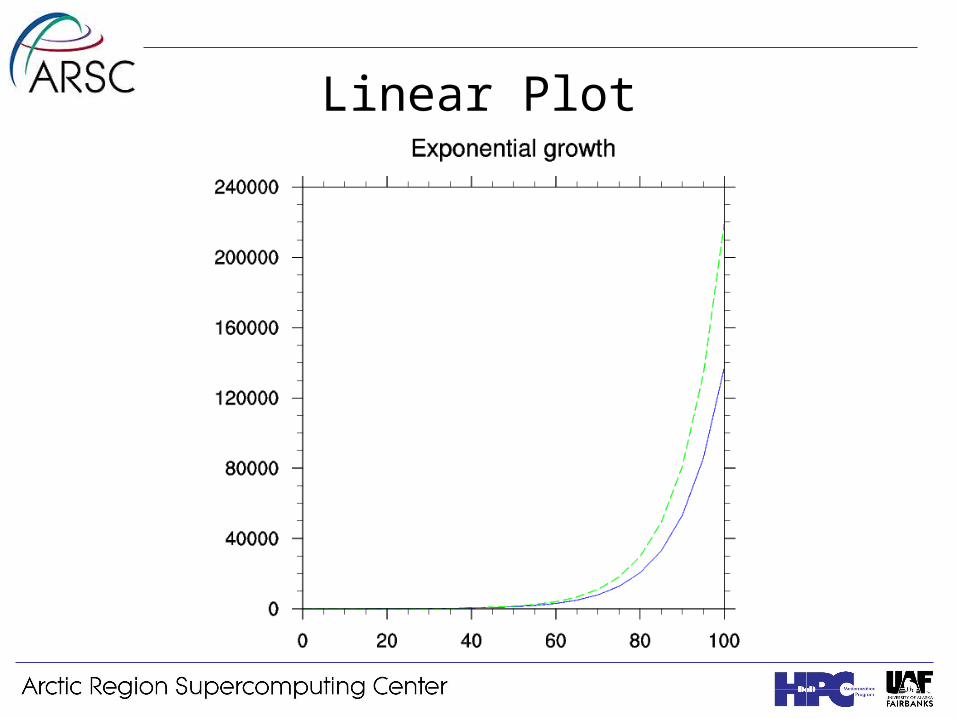
• Try b = 0.1, delta t = 1, initial N = 10• If the units are days, we have e times

more critters after 10 days• In the plot, green is the exact solution

while blue is the approximate solution using a one-day timestep

Linear Plot

Log Plot

Sources of Errors• Size of timestep relative to

timescales in the problem• Numerical scheme• Roundoff errors• How do you tell which is the trouble

here?• Since the numerical growth is also

exponential, we can adjust (tune) the time constant to obtain the correct solution

Two Species

• First rate equations for two species (one prey, one predator) were written by Lotka and Volterra during the 1920’s and 1930’s:

• Coupled, nonlinear, differential equations

• N1 is prey, N2 is predator, b, d, K1, K2 are constants, t is time

Assumptions

• Prey will grow exponentially without limit if no predators

• Rate of prey being eaten is proportional to the number of prey and the number of predators

• New predators happen immediately after eating prey

• No other prey options

Steady Solution

• No change in time:

• Trivial solution is N1 = N2 = 0

• Any solution satisfying the following is also steady:

Difference Equations• We can make an approximation to

the differential equations by assuming finite timesteps:

• These equations can be solved on a computer

• Need initial values for N1, N2, plus values for the constants

Numerical Solution

• One steady solution is given by N1=1000, N2=10, d=0.1, b=0.1, K1=0.01, K2=0.0001

• Using delta t =1, we get the steady solution numerically

• Any perturbation from the initial values for N1 and N2 will lead to expanding oscillations.

Initial N1=999

Initial N1=980

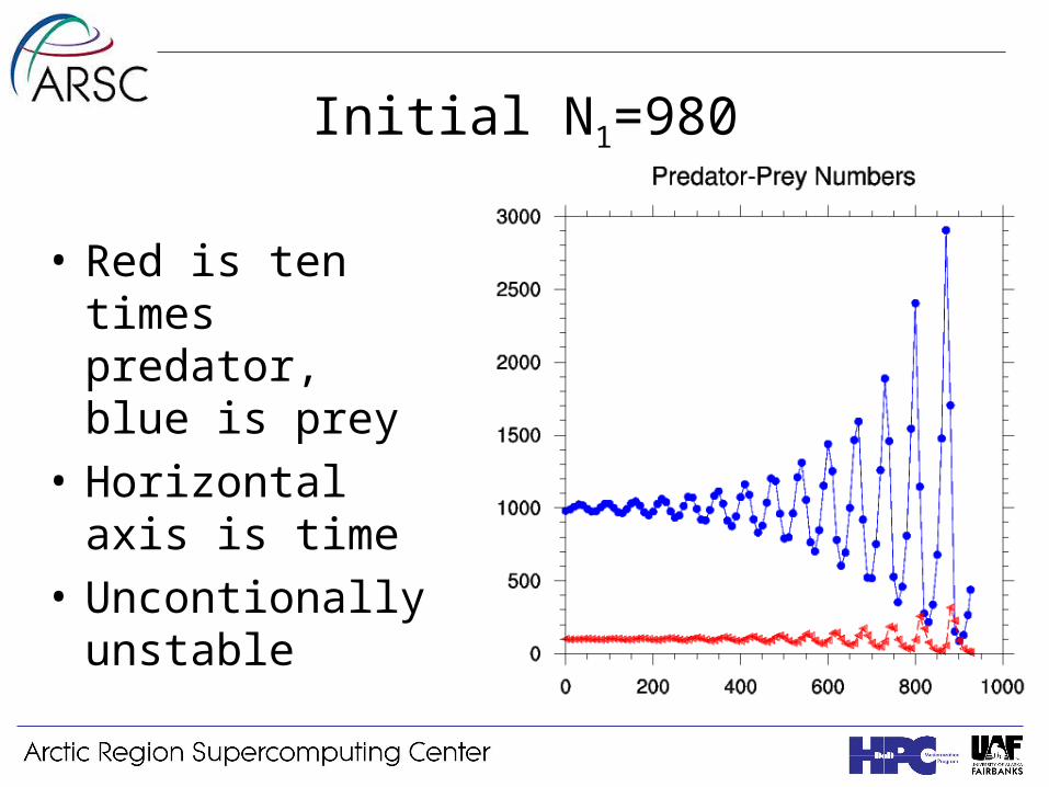
Initial N1=980

• Red is ten times predator, blue is prey

• Horizontal axis is time

• Uncontionally unstable

Why the instability?

• Invalid assumption in the equations– No limit to the number of prey supported– No alternate prey

• Unstable numerical scheme• Did you code it right?

Limit on the Prey

• Modifying the growth term for an environment that supports up to M prey:

• This equation is nonlinear, harder to solve exactly

• Growth rate becomes negative if N1 > M

One Species

Limiter in Lotka-Volterra Model

Lotka-Volterra PZ Model

• Same model as the original two component model:

• Different constants: P=N1=75, Z=N2=10, b=a=1, etc.

• Need a smaller timestep than one day for such large growth rates

dt=0.1 dt=0.001

Hmmm

• The author is obviously using dt=0.1• He then adds a Z cannibalism term to

damp the oscillations:

• This acts very much like the damper on the prey species

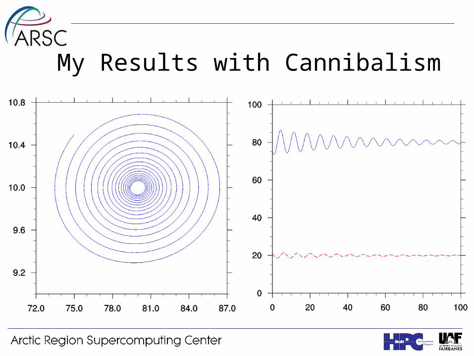
My Results with Cannibalism

Planetary Orbits

Euler Timestep and Orbits

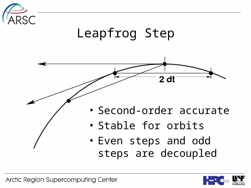
Leapfrog Step

• Second-order accurate• Stable for orbits• Even steps and odd steps

are decoupled

Timestepping Schemes

• Euler– Unconditionally unstable for some classes

of problems– Errors are linear in delta t (low order)

• Others– There are many, many other options– Some are higher order– Each has its own stability properties

Back to Lotka-Volterra

• Euler step, dt=0.01

Leapfrog-Trapezoidal Step

• Second-order accurate, more stable

Large Amplitude Cycles

Conclusions

• Lotka-Volterra is cyclic, not unstable• Simple-minded numerical schemes

can get us in trouble• Putting in more terms can lead to

realistic-looking results, such as the limits on exponential growth

• More complex ecosystem models still use Euler stepping with the damping terms

Questions

• Timestep vs. timestepping scheme• Data - growth rate data, say, to

improve or disprove a model• Error bars