economics partners, llc white paper · pdf fileeconomics partners, llc white paper series tim...

Capital Intensity and Margins

A Method for Analyzing Financial Comparability with Application to Distributors

Economics Partners, LLC

White Paper Series

Tim Reichert, Erin Hutchinson, and David Suhler

White Paper #2013-02


www.econpartners.com

Table of Contents

I. Introduction ................................................................................................................................... 1

II. The Fundamental Importance of Capital................................................................................... 3

A. Profit is the Return to Capital at Risk, Not Functions ....................................................... 3

B. Margins and Rates of Return ................................................................................................ 3

III. Application to the Berry Ratio .................................................................................................... 8

A. Definition and Characteristics of the Berry Ratio .............................................................. 8

B. Does the Relationship in Exhibit 3 Hold Empirically? .................................................... 10

1. Industry Scatterplot ....................................................................................................... 10

2. Econometric Tests .......................................................................................................... 11

C. Implications for the Comparable Profits Method ............................................................ 19

IV. Adjusting the Berry Ratio .......................................................................................................... 21

A. Comparison of Capital Intensity Ratios ............................................................................ 21

B. Arm’s Length Berry Ratio Estimate and Confidence Interval Ranges .......................... 23

V. Conclusion ................................................................................................................................... 25

Appendix A: Searches for Routine Distributors

Page | 1



ABSTRACT: This paper accomplishes three things. First, it examines the

economic meaning of the term “profit,” and its relationship to capital at

risk. A clear definition of profit is important in transfer pricing analysis,

because much confusion still exists regarding the precise relationship

between “functions,” “risks,” “assets,” and profit. We point out that

profit is always the return to at risk capital. In contrast to a common

misconception in the transfer pricing field, profit is never the return to

“functions.” Rather, profit is the return to the capital inputs (including

intangible capital inputs) employed in the performance of functions.

Second, we draw out the theoretical implications of this economic fact for

the use of margin measures (profit level indicators based upon sales or

costs). We show that under competitive conditions there is a linear

relationship between margins and capital intensity (capital / sales).

Finally, we test our theory using distributors, showing that the Berry ratio

and operating margin are in fact clearly and precisely related to the

capital employed to sales ratio. This allows us to: 1) much more

precisely measure the appropriate return to distribution activities, and 2)

make reliable adjustments to Berry ratios, cost plus markups, and

operating margins when benchmarking competitive activities such as

distribution and contract manufacturing.

I. Introduction

Taxpayers and tax authorities often employ the Comparable Profits Method (“CPM”) to test the

arm’s length nature of intercompany transactions. The CPM uses the profitability of

uncontrolled companies as an estimator of the profitability that would have inhered in one of

the controlled parties to an intercompany transaction (i.e., the “tested party”), had the tested

party transacted with its controlled affiliates at arm’s length. For example, in the case of a

controlled routine distributor, the comparison might be developed by identifying comparable

uncontrolled distributors, measuring their profitability using operating margins or Berry ratios,

and then applying this range of results to the tested party.

This sort of analysis obviously depends critically on what we mean by “comparability.” For the

most part, taxpayers and tax authorities emphasize “functional” comparability. That is,

comparability is defined along functional dimensions.

On the other hand, financial comparability tends to be ignored. While there seems to broad

agreement that financial comparability is theoretically important, no agreed upon definition of

financial comparability seems to exist.

The purpose of this paper is to offer a framework for thinking about financial comparability

across firms with similar functions. We show that taxpayers and tax authorities often apply the

Page | 2



CPM without recognizing the economic implications of the substantial difference between the

capital employed of the tested party and that of the comparable companies that are used in the

analysis. This creates a comparability problem, and can lead to unreliable results.

Specifically, we analyze and illustrate the fundamentally important financial implications of

differences in the intensity of operating capital employed and, in light of this, propose an

appropriate method for estimating arm’s length profitability that adjusts for such differences.

We use distributor returns to test our analysis and approach, in large part because distributor

returns are not strongly influenced by returns to intangible capital that can be difficult to

measure. However, our analysis and methodology is general, and can be applied to other types

of firms and activities.

This paper proceeds as follows. Section II outlines the core model that underlies this paper.

Section III then applies the theory from Section II to empirically estimate a model of the Berry

ratio. Section III specifies the model using both a broad sample of distributors, and an industry-

specific set of distributors, with very similar results in both cases. Section IV then applies the

model to a hypothetical distributor in order to estimate an arm’s length Berry ratio.

Page | 3



II. The Fundamental Importance of Capital

A. Profit is the Return to Capital at Risk, Not Functions

The most fundamental point in this paper is this – profit is always the return to capital. That

capital may be intangible capital or physical capital.

Profit is never, strictly speaking, a “markup on costs,” or a “margin on sales.” Profit may be

measured as a percentage of sales, total costs, or for that matter value added costs, but it is defined

as the return to investments in the capital employed by the firm.

Nor is profit, strictly speaking, a return to “functions.” Functions performed are the result of

both capital and labor inputs. Indeed, economic theory treats the firm as a “production

function,” involving labor inputs and capital inputs that are combined to produce an output of

some kind. Revenue earned by the firm, less its purchases from other firms, is distributed by

labor and capital markets to labor and capital inputs. Labor inputs are paid in the labor market,

at an arm’s length wage rate. Correspondingly, capital is “paid” in the capital markets, earning

profits (equity capital) or interest (debt capital). Thus, the statement commonly made by

transfer pricing professionals that profit is the return to functions performed is not strictly

speaking correct – profit is associated with functions performed, but it is in fact the payment to

the capital input used in support of the functions.

Operating profit, which is the subject of most transfer pricing analyses, is the return to the

firm’s operating assets, or equivalently to both equity and debt capital. This evident when one

examines the accounting equation (Assets = Debt + Equity). The accounting equation goes

somewhat further than economic theory (which, as noted, treats the firm as a specific

combination of capital and labor inputs). That is, the accounting equation states that the firm is

composed of assets – i.e., it is a portfolio of assets. These assets are financed by debt and equity.

Debt and equity are paid out of operating profit (if there is no operating profit, debt and equity

claimants do not earn a return) after labor inputs have been paid. Thus, even from the

perspective of accounting theory, we see that profit is the return to capital.1

B. Margins and Rates of Return

The fact that profit is the return to capital has important implications for how we think about

profit level indicators. Profit level indicators measure the ratio between profit and another

financial variable.

PLIs are divided into two categories: 1) margin measures, and 2) rates of return. Margin

measures examine the relationship between profit and an income statement variable such as

sales or costs. The most commonly used margin measures in the transfer pricing area include

1 It bears noting that operating profit also contains the return to “social capital,” paid in the form of taxes.

Page | 4



operating profit / sales (the operating margin, or “OM”), operating profit / total costs (the total

cost plus markup, or “CP”), and operating profit / operating expense (the Berry ratio).

Rates of return examine the relationship between profit and a measure of capital. The most

commonly used rates of return in the transfer pricing area are operating profit / operating assets

(the operating rate of return, or “ORR”), and operating profit / capital employed (the return on

capital employed, or “ROCE”).

An important requirement for a PLI to be a meaningful and reliable way to measure and

compare the profits of firms is that the numerator (the profit measure) logically correspond to, or

relate to, the denominator. That is, there must be some kind of expected economic relationship,

or regularity, between the numerator and denominator. If there is no such regularity, then by

definition the profit measure is not measuring a relationship. Rather, what is being measured is

just a random ratio, which implies that comparisons across firms will not be meaningful.

An example of a PLI for which there is no economic relationship (or virtually none) between the

numerator and denominator is Gross Profit / Depreciation. Presumably, this ratio strikes the

reader as odd – precisely because it is odd. Gross Profit simply bears very little relationship to

Depreciation. Therefore, this PLI is seldom (if ever) used.

In general, the more direct, or causal, is the relationship between the profit measure in the

numerator and the variable in the denominator, the more reliable and meaningful is the PLI.

The ideal PLI contains a numerator that is economically caused by the variable in the

denominator.

Returning to the idea that profit is the return to capital, it should be apparent that rates of return

have a certain logical correspondence between numerator and denominator that margin

measures do not. Because profit is the return to capital, profit level indicators in which the

denominator is a capital measure (i.e., rates of return) directly capture the causal link between

profit and capital in a way that margin measures cannot. All else equal, rates of return are to be

preferred to margin measures.2

The advantages that stem from this causal correspondence between numerator and

denominator are reflected in the US transfer pricing regulations. In discussing the Comparable

Profits Method, which compares the profit of one party to a transaction (i.e., the tested party) to

the profits of a sample of comparable companies, the regulations state that, all else equal, the

use of asset-based PLIs (rates of return) should reduce (though not eliminate) the need for

comparability across the firms in a sample, and between the sample and the tested party.3 This

makes sense. If profit is the return to capital (i.e., assets), then comparing the returns to assets is

2 The caveat “all else equal” is critical here. In practice it may frequently be the case that margin measures are inherently more reliable, or preferable, to rates of return. For example, in cases where capital investments are extremely lumpy through time, a measure for a given period may understate or overstate capital in a steady state sense. By contrast, margin measures in such a case represent flows of income and revenue or costs. Such flows may be much less lumpy, and may therefore produce a more reliable PLI than a rate of return. 3 See Section 482-5(b)(4)(ii).

Page | 5



a more direct way to understand the profitability of firms than, say, comparing margins on

sales.

Thus, relative to rates of return, the causal link between numerator and denominator is not as

direct or clear for margin measures as it is for rates of return. More precisely, without

appropriate adjustment, margin measures blur the causality between numerator and

denominator because, as we will see directly below, every margin measure mathematically

reduces to a rate of return measure times an “asset intensity ratio.” That is, margin measures

are simply rates of return times an asset intensity measure. This means that a direct comparison

(i.e., a comparison without appropriate adjustment) using margin measures, of firms with

different asset intensities may not be reliable.

The asset intensity ratio is simply the ratio of assets or capital to sales or costs. It is therefore a

measure of how many dollars of assets are required to yield a dollar of sales, or how many

dollars of assets are associated with a dollar of costs. It is thus an efficiency measure. Firms

with fewer dollars of assets per dollar of sales or costs are more efficient at converting their

capital into revenue. Correspondingly, firms with more capital per dollar of revenue are

obviously less efficient.

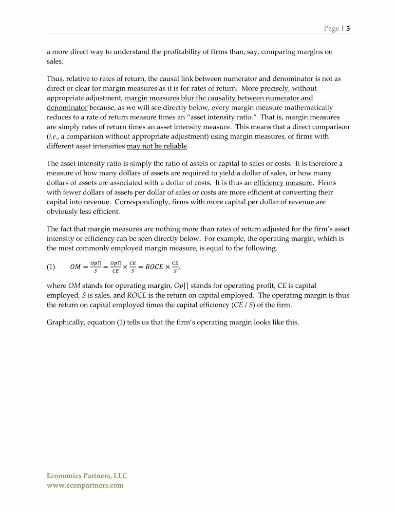
The fact that margin measures are nothing more than rates of return adjusted for the firm’s asset

intensity or efficiency can be seen directly below. For example, the operating margin, which is

the most commonly employed margin measure, is equal to the following.

(1)

,

where OM stands for operating margin, Op∏ stands for operating profit, CE is capital

employed, S is sales, and ROCE is the return on capital employed. The operating margin is thus

the return on capital employed times the capital efficiency (CE / S) of the firm.

Graphically, equation (1) tells us that the firm’s operating margin looks like this.

Page | 6



Exhibit 1

OM is ROCE × Capital Intensity

Exhibit 1 tells us two important things. First, because the operating margin is simply the firm’s

ROCE times its asset intensity, the OM is linearly increasing as asset intensity increases.

Moreover, interestingly, the rate of increase in OM as capital intensity increases is the firm’s

ROCE. In other words, all firms on the OM line shown in Exhibit 1 will have the same ROCE,

but have very different operating margins. This is a very useful relationship, and as we will see

one that allows us to make adjustments to OMs (or margin measures generally) to enhance their

reliability.

Second, and more importantly, Exhibit 1 tells us that two firms that are otherwise functionally

comparable, but that have different asset intensities, will have very different operating margins.

Returning for a moment to the economic view of the firm as a production function, firms that

substitute capital for labor in order to produce output should, all else equal, have higher

operating margins than firms that substitute labor for capital.

This means that if we have two firms with very different asset intensities, and if one of these

firms is a tested party and the other is a “comparable,” and we apply the comparable firm’s OM

to the tested party, we will inadvertently shift shareholder value (economic profit) to or from

the tested party. This would be an uncompensated value leakage, and inconsistent with the

arm’s length principle.

The preceding sentence may not be immediately obvious. The reader may ask, “why would

this be a violation of the arm’s length principle?” The answer is simple, and rests on one of the

most fundamental concepts in economics – the concept of “value.” Value is merely something

that someone would pay for.

Bringing this back to Exhibit 1, we see that firms that have high OMs are likely to have high

OMs because they are capital intensive. They need more operating profit per dollar of sales

because they have more capital per dollar of sales, and this capital (like labor) must be paid. If

we were to apply the high OM from a capital intensive firm to a tested party with very little in

OM = ROCE x (CE/S)

-- Slope of Line = ROCE

OM

CE/S

Page | 7



the way of capital, we would by definition overcompensate that tested party’s capital base. In

other words, the low capital tested party would earn more profit than its capital inputs actually

require. This excess profit is an overcompensation of the tested party’s capital base, and since

profit is the return to capital, this is by definition excess profit to the tested party. This excess

profit is by definition something that has value, as it represents excess cash flow that is available

to the tested party but that was unavailable to the comparable. That is, the comparable needed

all of the operating margin (all of the operating profit per dollar of sales) to cover its capital

costs, because it had more capital per dollar of sales. By contrast, the tested party, with less

capital, needs less operating profit per dollar of sale, implying that the excess compensation is a

“free lunch” in the form of “free” cash flow.

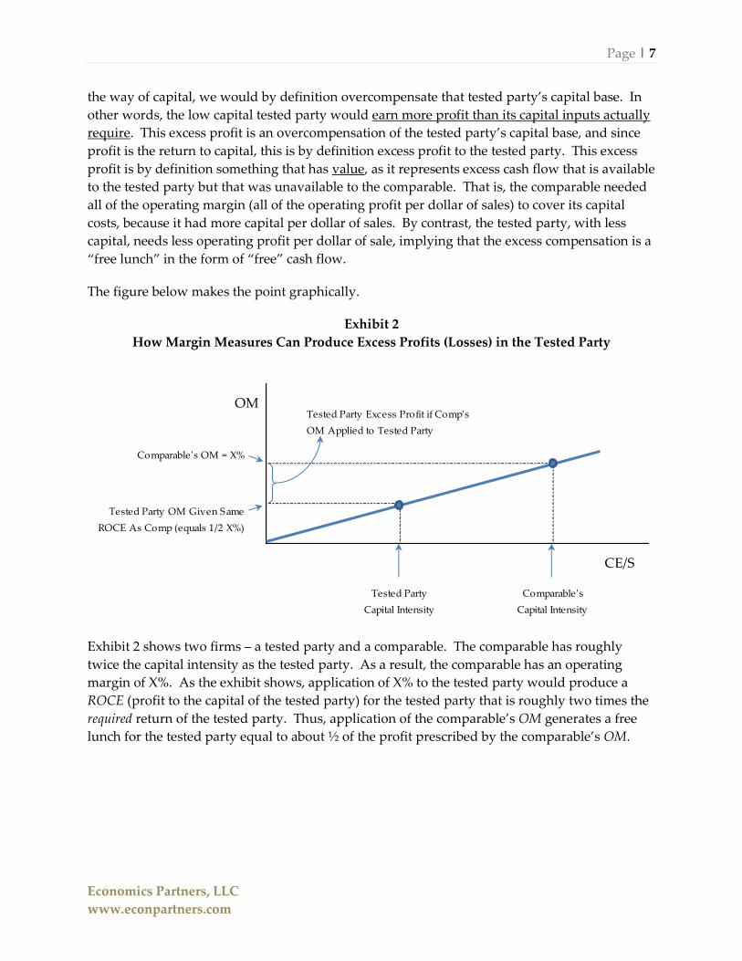
The figure below makes the point graphically.

Exhibit 2

How Margin Measures Can Produce Excess Profits (Losses) in the Tested Party

Exhibit 2 shows two firms – a tested party and a comparable. The comparable has roughly

twice the capital intensity as the tested party. As a result, the comparable has an operating

margin of X%. As the exhibit shows, application of X% to the tested party would produce a

ROCE (profit to the capital of the tested party) for the tested party that is roughly two times the

required return of the tested party. Thus, application of the comparable’s OM generates a free

lunch for the tested party equal to about ½ of the profit prescribed by the comparable’s OM.

Comparable's OM = X%

Tested Party Excess Profit if Comp's

OM Applied to Tested Party

OM

CE/S

Comparable's

Capital Intensity

Tested Party

Capital Intensity

Tested Party OM Given Same

ROCE As Comp (equals 1/2 X%)

Page | 8



III. Application to the Berry Ratio

A. Definition and Characteristics of the Berry Ratio

The Berry ratio (“Berry”) was first introduced by Dr. Charles Berry in the transfer pricing court

case E.I. DuPont de Nemours v. United States. Dr. Berry ratio introduced the ratio (defined

directly below) as a profit level indicator for use by transfer pricing analysts in measuring and

comparing the returns earned by distributors.

The Berry is defined as gross profit / operating expenses. Mathematically, the Berry ratio

reduces to 1 + M, where M is operating profit / operating expenses, or the “markup” on

operating expenses. Equation (2) summarizes the Berry ratio.

(2)

In equation (2) B is the Berry ratio, G∏ is gross profit, Op∏ is operating profit, OpX is operating

expense, and M is the markup on operating expense (Op∏ / OpX).

The reasoning behind the Berry ratio is straightforward. For some firms, particularly

distributors, most or all of their cost of goods sold (“COGS”) is a “pass through,” meaning that

the COGS represents the arm’s length value of the labor and capital inputs used by third party

suppliers to produce the goods that the distributor has purchased. By contrast, operating

expense (OpX) represents the “value added cost,” or the cost associated with the value that the

distributor adds to the economy. Since the market prices paid to a firm for its goods and

services are the reward to the firms for its own capital and labor inputs, rather than its suppliers

capital and labor inputs, focusing attention on value added cost provides a correspondence of

sorts between the numerator and denominator of the ratio. That is, the numerator of the Berry

(G∏) is the portion of the distributor’s revenue that rewards the distributor for its “value add,”

and the denominator (OpX) is that value add. By maintaining this correspondence between the

numerator and denominator, the Berry ratio is superior to its primary margin measure

alternatives, the operating margin and the total cost plus markup (“CP”).

Nonetheless, as a margin measure, the Berry ratio has the same deficiencies related to capital

intensity as other margin measures. This can be seen directly below in equation (3).

(3)

where all variables are defined as before. Equation (3) is essentially the same as equation (1),

with some modifications that are pertinent to distributors. Specifically, because the Berry ratio

is defined to equal 1 + M, the intercept of the line given in equation (3) is equal to 1. In addition,

capital intensity is defined relative to operating expenses, rather than sales. Exhibit 3 shows this

relationship graphically.

Page | 9



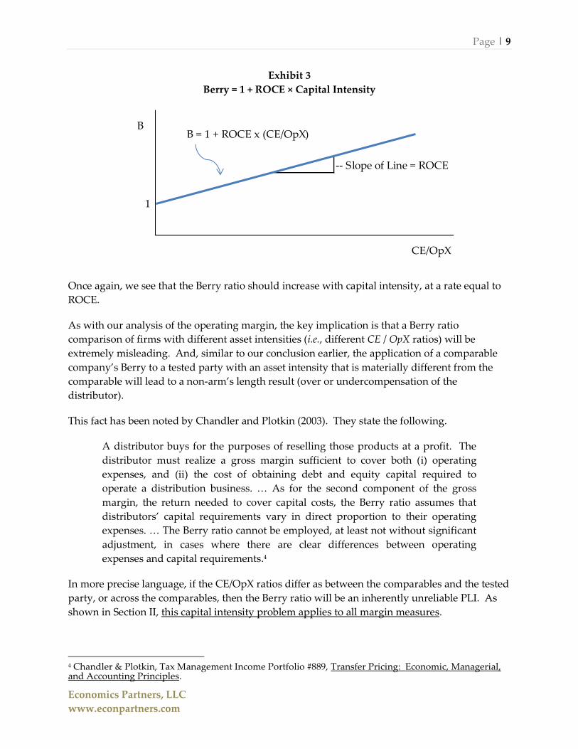
Exhibit 3

Berry = 1 + ROCE × Capital Intensity

Once again, we see that the Berry ratio should increase with capital intensity, at a rate equal to

ROCE.

As with our analysis of the operating margin, the key implication is that a Berry ratio

comparison of firms with different asset intensities (i.e., different CE / OpX ratios) will be

extremely misleading. And, similar to our conclusion earlier, the application of a comparable

company’s Berry to a tested party with an asset intensity that is materially different from the

comparable will lead to a non-arm’s length result (over or undercompensation of the

distributor).

This fact has been noted by Chandler and Plotkin (2003). They state the following.

A distributor buys for the purposes of reselling those products at a profit. The

distributor must realize a gross margin sufficient to cover both (i) operating

expenses, and (ii) the cost of obtaining debt and equity capital required to

operate a distribution business. … As for the second component of the gross

margin, the return needed to cover capital costs, the Berry ratio assumes that

distributors’ capital requirements vary in direct proportion to their operating

expenses. … The Berry ratio cannot be employed, at least not without significant

adjustment, in cases where there are clear differences between operating

expenses and capital requirements.4

In more precise language, if the CE/OpX ratios differ as between the comparables and the tested

party, or across the comparables, then the Berry ratio will be an inherently unreliable PLI. As

shown in Section II, this capital intensity problem applies to all margin measures.

4 Chandler & Plotkin, Tax Management Income Portfolio #889, Transfer Pricing: Economic, Managerial, and Accounting Principles.

B = 1 + ROCE x (CE/OpX)

-- Slope of Line = ROCE

B

CE/OpX

1

Page | 10



B. Does the Relationship in Exhibit 3 Hold Empirically?

1. Industry Scatterplot

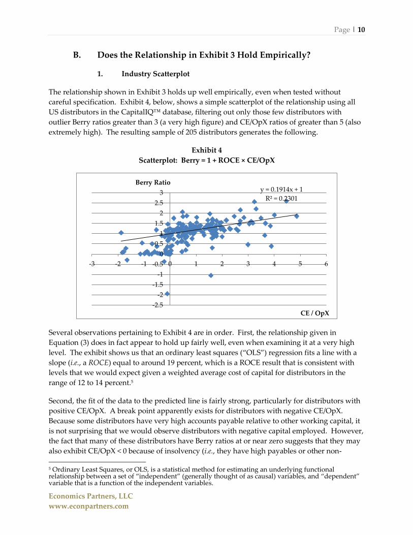
The relationship shown in Exhibit 3 holds up well empirically, even when tested without

careful specification. Exhibit 4, below, shows a simple scatterplot of the relationship using all

US distributors in the CapitalIQ™ database, filtering out only those few distributors with

outlier Berry ratios greater than 3 (a very high figure) and CE/OpX ratios of greater than 5 (also

extremely high). The resulting sample of 205 distributors generates the following.

Exhibit 4

Scatterplot: Berry = 1 + ROCE × CE/OpX

Several observations pertaining to Exhibit 4 are in order. First, the relationship given in

Equation (3) does in fact appear to hold up fairly well, even when examining it at a very high

level. The exhibit shows us that an ordinary least squares (“OLS”) regression fits a line with a

slope (i.e., a ROCE) equal to around 19 percent, which is a ROCE result that is consistent with

levels that we would expect given a weighted average cost of capital for distributors in the

range of 12 to 14 percent.5

Second, the fit of the data to the predicted line is fairly strong, particularly for distributors with

positive CE/OpX. A break point apparently exists for distributors with negative CE/OpX.

Because some distributors have very high accounts payable relative to other working capital, it

is not surprising that we would observe distributors with negative capital employed. However,

the fact that many of these distributors have Berry ratios at or near zero suggests that they may

also exhibit CE/OpX < 0 because of insolvency (i.e., they have high payables or other non-

5 Ordinary Least Squares, or OLS, is a statistical method for estimating an underlying functional relationship between a set of “independent” (generally thought of as causal) variables, and “dependent” variable that is a function of the independent variables.

y = 0.1914x + 1

R² = 0.2301

-2.5

-2

-1.5

-1

-0.5

0

0.5

1

1.5

2

2.5

3

-3 -2 -1 0 1 2 3 4 5 6

Berry Ratio

CE / OpX

Page | 11



interest bearing liabilities that offset their operating assets, and these high payables balances

occur as a result of not being able to pay suppliers). Therefore, for purposes of our more formal

econometric specifications discussed later, there should be some accounting for this problem.

Finally, it appears that the variance in the Berry ratios rises sharply at CE/OpX levels of around

3. This may be because very high levels of capital employed relative to OpX can signal both

inefficiency (i.e., too many assets chasing not enough revenue) and efficiency (in the form of

capital for labor substitution).

2. Econometric Tests

We also tested this relationship more formally (i.e., econometrically), using a broad sample of

US distributors in the CapitalIQ™ database and an industry-specific set of distributors. The

industry that we elected to use as an example is the computers and electronics distribution

industry. The broad distributor set contains 159 companies, and the industry-specific set

contains 12 companies. For a description of the search processes that were used to identify the

two sets of companies, please see Appendix A.

The purpose of our analysis was to quantitatively examine the arm’s length, or market-implied,

relationship between CE/OpX and profitability. To do so, we employed an ordinary least

squares regression method to estimate the relationship between the Berry ratio and CE/OpX

described in Equation 3 and illustrated in Exhibit 3. OLS is an econometric technique used to

estimate the relationship between two (or more) variables by computing the intercept and slope

of a line that best fits the data. This line of best fit is the line that minimizes the sum of squared

distances between the line and the individual data points. The sections that follow present our

econometric analysis.

(1) Data

As mentioned above, our search process for the full sample resulted in 159 companies. These

companies operate across eight distribution industry classifications. Industry classifications

were assigned by CapitalIQ™ using the Standard Industrial Classification (“SIC”) system. A

description of these industry classifications is given in Exhibit 5 below.

Page | 12



Exhibit 5 – Industry Classification

Given financial data for 159 companies, one could construct a “cross-sectional” data set using

the Berry ratios and CE/OpX of these 159 companies at a given point in time. However, cross-

sectional data sets do not control for year over year differences in a firm’s financial performance

that result from factors specific to a certain time period. That is, a firm’s single-year observation

may reflect a poor business year, yielding a much different result than if we chose a year where

the firm was highly profitable. In order to mitigate the influence of a single year’s results, we

can instead construct a time series for each company by observing its Berry ratio and CE/OpX

over time. By observing each company over time, we can control for year-by-year differences in

the company while also increasing our sample size. Thus, we constructed a “panel” data set,

wherein each annual observation for each company represents a separate “firm-year”

observation. Each firm-year observation represents a given company’s Berry ratio, CE/OpX

ratio, and industry classification for a given year6. We used annual observations over 8 years, so

our full sample consisted of 1,272 firm-year observations (i.e., 159 companies * 8 years = 1,272

firm-year observations).

We then removed all firm-year observations with non-positive Berry ratios and CE/OpX7 ratios.

The resulting panel data set included 965 firm-year observations.

6 A firm’s Berry ratio and CE/OpX ratio vary over time, but their industry classification is constant over time. That is, while a company’s profitability and capital intensity will be different in each year, the company does not change industries. 7 We made an adjustment to net PP&E for companies that employ operating leases. Since operating leases are a form of off-balance sheet financing, companies who use operating leases will understate the amount of capital employed by the value of the assets being leased. We use a standard adjustment that calculates the value of the asset leased as the net rental expense multiplied by eight. We then add this estimated asset value to the balance sheet of the company by increasing the PP&E by that amount. Additionally, the net rental expense incurred by the company has two components: a depreciation component and an implied interest component. If a company owned the asset outright, it would only recognize the depreciation component within OpX, with the interest component being recognized after operating profit

Industry SIC Codes

Electronics, Software and

General Technology5045, 506*

Capital Goods and Raw

Materials

5046, 5051, 5093, 5110,

503*, 507*, 508*, 516*

Food, Beverage and other non-

durables5153, 514*, 518*, 519*

Consumer Durables5000, 5014, 502*, 509*,

513*

Healthcare 5040, 5047, 5122

Energy 5171, 5172

Automobile 5010, 5012, 5013

Agriculture 5150, 5191

Page | 13



Equation (4) represents the line we estimated for the full sample.

(4)

Where is the Berry ratio for a given firm, c, in year t. In the full sample, there were

159 firms, so c ranges from 1 to 159. Similarly, there were 8 years of data observed, so t ranges

from 1 to 8. is an industry-specific “fixed effect” (binary, or zero-one, variable) that captures

variation across industry that is not explained by another variable in the model (essentially,

fixed effects estimation creates a dummy variable for each industry).

To follow the theoretical foundation presented in equation (3), we forced the general intercept

of the Berry ratio line, or function, to equal one. Forcing the intercept to one allows the industry

dummy variable, or industry fixed effect, to represent an industry-specific upward shift to the

Berry ratio equation given in equation (3). This upward shift will vary by industry, which

implies that one plus the industry dummy creates a specific intercept estimate for each industry

(i.e., is the intercept for industry i). Allowing the intercept to vary by industry produces

a single estimate for ROCE that is the same for all distribution sectors (industries). In a fixed

effects OLS regression, the reported coefficient on ROCE represents the average effect of that

variable on profitability across all industries. Since there were 8 industries included in this

sample, i ranges from 1 to 8. is our parameter of interest, and it represents the ROCE. Finally,

is the random error term. The following table provides descriptive statistics for the full

sample.

is calculated. Therefore, we remove the interest component of the net rental expense in the calculation of OpX.

Page | 14



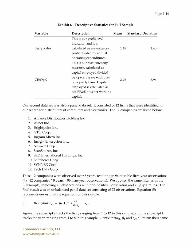
Exhibit 6 – Descriptive Statistics for Full Sample

Our second data set was also a panel data set. It consisted of 12 firms that were identified in

our search for distributors of computers and electronics. The 12 companies are listed below.

1. Alliance Distributors Holding Inc.

2. Avnet Inc.

3. Brightpoint Inc.

4. GTSI Corp.

5. Ingram Micro Inc.

6. Insight Enterprises Inc.

7. Navarre Corp.

8. ScanSource, Inc.

9. SED International Holdings, Inc.

10. Softchoice Corp.

11. SYNNEX Corp.

12. Tech Data Corp.

These 12 companies were observed over 8 years, resulting in 96 possible firm-year observations

(i.e., 12 companies * 8 years = 96 firm-year observations). We applied the same filter as in the

full sample, removing all observations with non-positive Berry ratios and CE/OpX ratios. The

final result was an unbalanced panel data set consisting of 72 observations. Equation (5)

represents our estimating equation for this sample.

(5)

Again, the subscript c tracks the firm, ranging from 1 to 12 in this sample, and the subscript t

tracks the year, ranging from 1 to 8 in this sample. , and all retain their same

Variable Description Mean Standard Deviation

Berry Ratio

This is our profit level

indicator, and it is

calculated as annual gross

profit divided by annual

operating expenditures.

1.48 1.43

CE/OpX

This is our asset intensity

measure, calculated as

capital employed divided

by operating expenditures

on a yearly basis. Capital

employed is calculated as

net PP&E plus net working

capital.

2.96 6.96

Page | 15



definitions as before. We did not fix the intercept to one, so is the estimated general intercept

for all firms. All firms in the industry sample fall into the same industry classification

(Electronics, Software and General Technology). Since all firms in this set are in the same

industry, there is no need to estimate industry-specific fixed effects in this model. The general

intercept term in this model is the industry specific intercept.

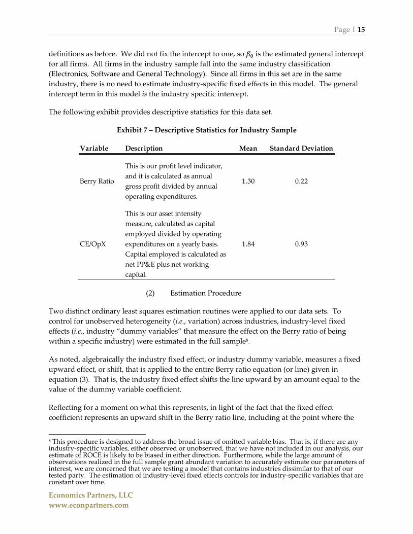
The following exhibit provides descriptive statistics for this data set.

Exhibit 7 – Descriptive Statistics for Industry Sample

(2) Estimation Procedure

Two distinct ordinary least squares estimation routines were applied to our data sets. To

control for unobserved heterogeneity (i.e., variation) across industries, industry-level fixed

effects (i.e., industry “dummy variables” that measure the effect on the Berry ratio of being

within a specific industry) were estimated in the full sample8.

As noted, algebraically the industry fixed effect, or industry dummy variable, measures a fixed

upward effect, or shift, that is applied to the entire Berry ratio equation (or line) given in

equation (3). That is, the industry fixed effect shifts the line upward by an amount equal to the

value of the dummy variable coefficient.

Reflecting for a moment on what this represents, in light of the fact that the fixed effect

coefficient represents an upward shift in the Berry ratio line, including at the point where the

8 This procedure is designed to address the broad issue of omitted variable bias. That is, if there are any industry-specific variables, either observed or unobserved, that we have not included in our analysis, our estimate of ROCE is likely to be biased in either direction. Furthermore, while the large amount of observations realized in the full sample grant abundant variation to accurately estimate our parameters of interest, we are concerned that we are testing a model that contains industries dissimilar to that of our tested party. The estimation of industry-level fixed effects controls for industry-specific variables that are constant over time.

Variable Description Mean Standard Deviation

Berry Ratio

This is our profit level indicator,

and it is calculated as annual

gross profit divided by annual

operating expenditures.

1.30 0.22

CE/OpX

This is our asset intensity

measure, calculated as capital

employed divided by operating

expenditures on a yearly basis.

Capital employed is calculated as

net PP&E plus net working

capital.

1.84 0.93

Page | 16



intercept at which the CE of the firm is zero, this fixed effect must represent the profitability

attributable to non-financial and non-physical capital. That is, the industry dummy variable

must be measuring the returns to intangible capital. This fact is most obvious at the intercept,

where CE/OpX is zero. At a zero CE, firms should earn a Berry ratio of 1 – meaning operating

profit of zero – absent a return to other forms of capital such as intangible capital. However,

our quantitative model shows that firms do not earn a Berry of 1 at zero CE. The reason for this

is that distributors often do in fact own intangible assets such as customer relationships and

customer lists. In short, then, the fixed effect is the return attributable to customer-based

intangibles (and possibly other intangibles owned by distributors) within a given industry

classification.

Again, it bears noting that in the industry sample, every company in these sets is also within the

same industry. Thus, fixed effects estimation did not apply to these data sets. Estimation of the

ROCE in these samples was accomplished via ordinary least squares.

(3) Regression Results

The regression results for our two data sets are presented in the exhibits below.

Page | 17



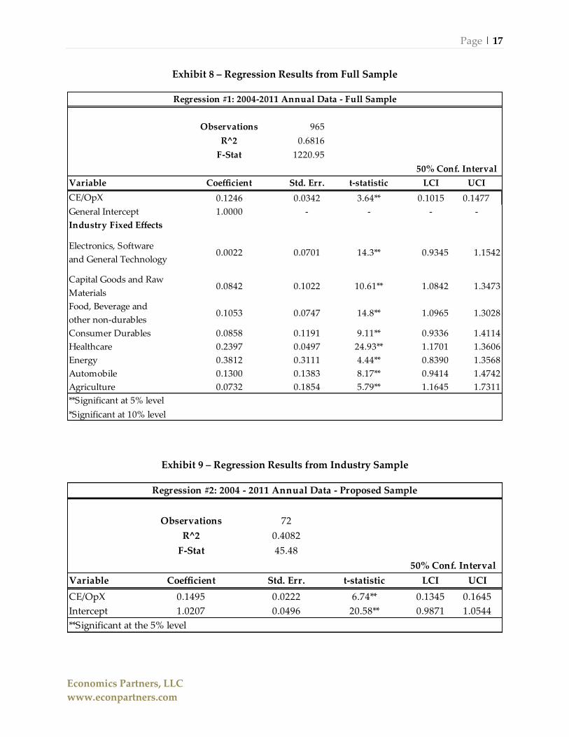
Exhibit 8 – Regression Results from Full Sample

Exhibit 9 – Regression Results from Industry Sample

Regression #1: 2004-2011 Annual Data - Full Sample

Observations 965

R^2 0.6816

F-Stat 1220.95

50% Conf. Interval

Variable Coefficient Std. Err. t-statistic LCI UCI

CE/OpX 0.1246 0.0342 3.64** 0.1015 0.1477

General Intercept 1.0000 - - - -

Industry Fixed Effects

Electronics, Software

and General Technology0.0022 0.0701 14.3** 0.9345 1.1542

Capital Goods and Raw

Materials0.0842 0.1022 10.61** 1.0842 1.3473

Food, Beverage and

other non-durables0.1053 0.0747 14.8** 1.0965 1.3028

Consumer Durables 0.0858 0.1191 9.11** 0.9336 1.4114

Healthcare 0.2397 0.0497 24.93** 1.1701 1.3606

Energy 0.3812 0.3111 4.44** 0.8390 1.3568

Automobile 0.1300 0.1383 8.17** 0.9414 1.4742

Agriculture 0.0732 0.1854 5.79** 1.1645 1.7311

**Significant at 5% level

*Significant at 10% level

Regression #2: 2004 - 2011 Annual Data - Proposed Sample

Observations 72

R^2 0.4082

F-Stat 45.48

50% Conf. Interval

Variable Coefficient Std. Err. t-statistic LCI UCI

CE/OpX 0.1495 0.0222 6.74** 0.1345 0.1645

Intercept 1.0207 0.0496 20.58** 0.9871 1.0544

**Significant at the 5% level

Page | 18



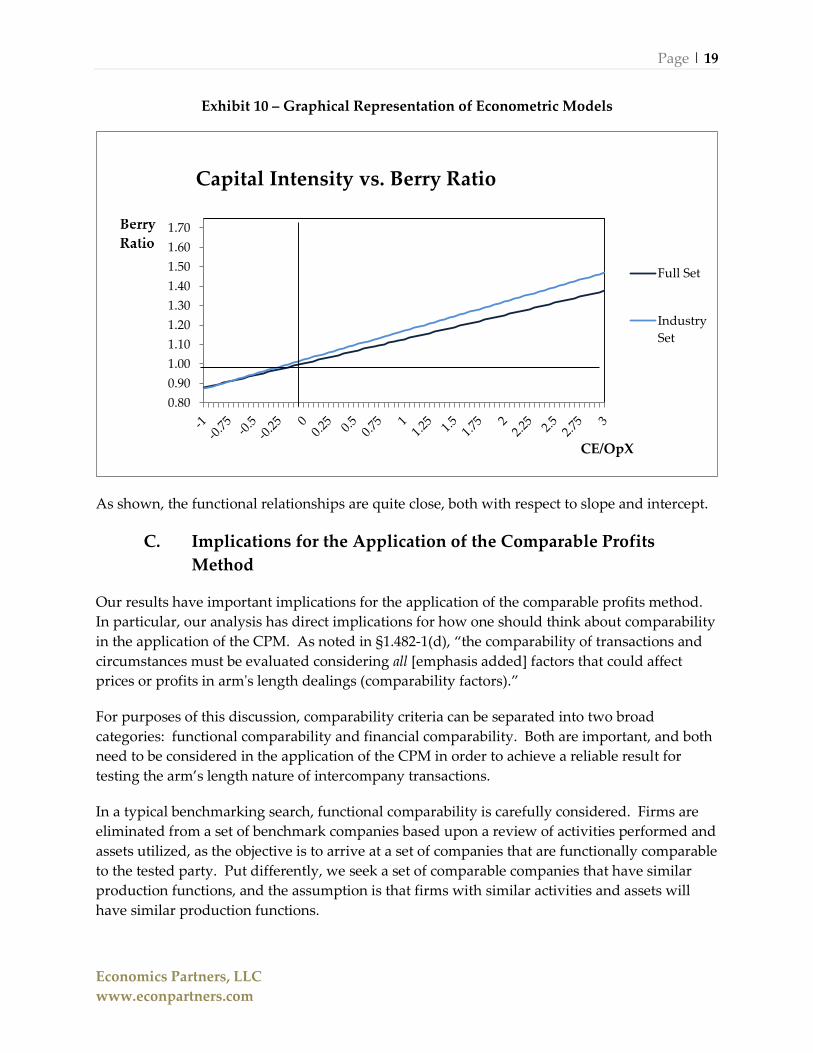
Several observations regarding our econometric results are in order. First, of the statistics

shown in the preceding exhibits, the R2 is perhaps the most important. The R2 represents the

percentage of the variation in the Berry ratio data that is explained by our econometric model –

i.e., the percentage of the variation that is explained by Capital Employed. Our models clearly

have a significant amount of explanatory power, with measures of 68 percent in the case of

the full sample, and 41 percent in the case of the industry sample. The R2 is higher in the full

model, and this can most likely be attributed to the larger sample size and the explanatory

power of the industry-level fixed effects. However, even the much smaller industry set

performs well – exhibiting a very respectable R2 of approximately 41 percent.

It is also worth examining the ROCE estimate for the two models. The full sample tells us that

the ROCE for distributors is approximately 12.46 percent, while the industry sample produces

an estimate of ROCE at 14.95 percent. These figures are quite similar, and are both consistent

with our expectation that distributors should earn returns on capital employed that are

consistent with their cost of capital.

Finally, the F-statistic represents a hypothesis test of overall significance of each econometric

model. Essentially, the F-statistic is a test to verify that the entire set of estimated coefficients in

each model – or said differently, the model as a whole – is statistically significant. If an

econometric model “fails the F-test,” the model is indistinguishable from randomness, and is

therefore a meaningless model. In each of our models, the F-statistics were extremely high, and

we can say that with 99 percent confidence that our models estimated statistically significant

coefficients.

To illustrate the functional relationships predicted by our econometric models, we generated

the following simple graph.

Page | 19



Exhibit 10 – Graphical Representation of Econometric Models

As shown, the functional relationships are quite close, both with respect to slope and intercept.

C. Implications for the Application of the Comparable Profits

Method

Our results have important implications for the application of the comparable profits method.

In particular, our analysis has direct implications for how one should think about comparability

in the application of the CPM. As noted in §1.482-1(d), “the comparability of transactions and

circumstances must be evaluated considering all [emphasis added] factors that could affect

prices or profits in arm's length dealings (comparability factors).”

For purposes of this discussion, comparability criteria can be separated into two broad

categories: functional comparability and financial comparability. Both are important, and both

need to be considered in the application of the CPM in order to achieve a reliable result for

testing the arm’s length nature of intercompany transactions.

In a typical benchmarking search, functional comparability is carefully considered. Firms are

eliminated from a set of benchmark companies based upon a review of activities performed and

assets utilized, as the objective is to arrive at a set of companies that are functionally comparable

to the tested party. Put differently, we seek a set of comparable companies that have similar

production functions, and the assumption is that firms with similar activities and assets will

have similar production functions.

0.80

0.90

1.00

1.10

1.20

1.30

1.40

1.50

1.60

1.70

Capital Intensity vs. Berry Ratio

Full Set

Industry

Set

CE/OpX

Page | 20



However, this type of functional review ignores the fact that the capital intensity ratios for the

potentially comparable companies might vary considerably. Even given identical production

functions, two firms facing different external constraints (e.g., labor and capital costs) may

substitute capital for labor, or vice-versa. The results of our theoretical and empirical analyses

demonstrate that differences in capital intensity fundamentally impact a firm’s profits, and

therefore such differences must be accounted for in the application of any transfer pricing

method, particularly a profit-based method such as the CPM.

As discussed earlier, ignoring capital intensity can lead to overcompensating (or

undercompensating) a tested party depending upon its capital intensity ratio relative to

benchmark companies. Since profit is a return to capital, a margin measure such as the Berry

ratio must be appropriately adjusted for differences in capital intensity if it is to be used as a

reliable measure for an arm’s length return. In what follows, we use the results of the

regression analysis to properly adjust the Berry ratio results of the comparable companies to

account for differences between their capital intensity and a hypothetical tested party’s capital

intensity.

Page | 21



IV. Adjusting the Berry Ratio

A. Comparison of Capital Intensity Ratios

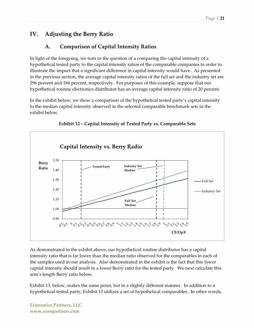
In light of the foregoing, we turn to the question of a comparing the capital intensity of a

hypothetical tested party to the capital intensity ratios of the comparable companies in order to

illustrate the impact that a significant difference in capital intensity would have. As presented

in the previous section, the average capital intensity ratios of the full set and the industry set are

296 percent and 184 percent, respectively. For purposes of this example, suppose that our

hypothetical routine electronics distributor has an average capital intensity ratio of 20 percent.

In the exhibit below, we show a comparison of the hypothetical tested party’s capital intensity

to the median capital intensity observed in the selected comparable benchmark sets in the

exhibit below.

Exhibit 12 – Capital Intensity of Tested Party vs. Comparable Sets

As demonstrated in the exhibit above, our hypothetical routine distributor has a capital

intensity ratio that is far lower than the median ratio observed for the comparables in each of

the samples used in our analysis. Also demonstrated in the exhibit is the fact that this lower

capital intensity should result in a lower Berry ratio for the tested party. We next calculate this

arm’s length Berry ratio below.

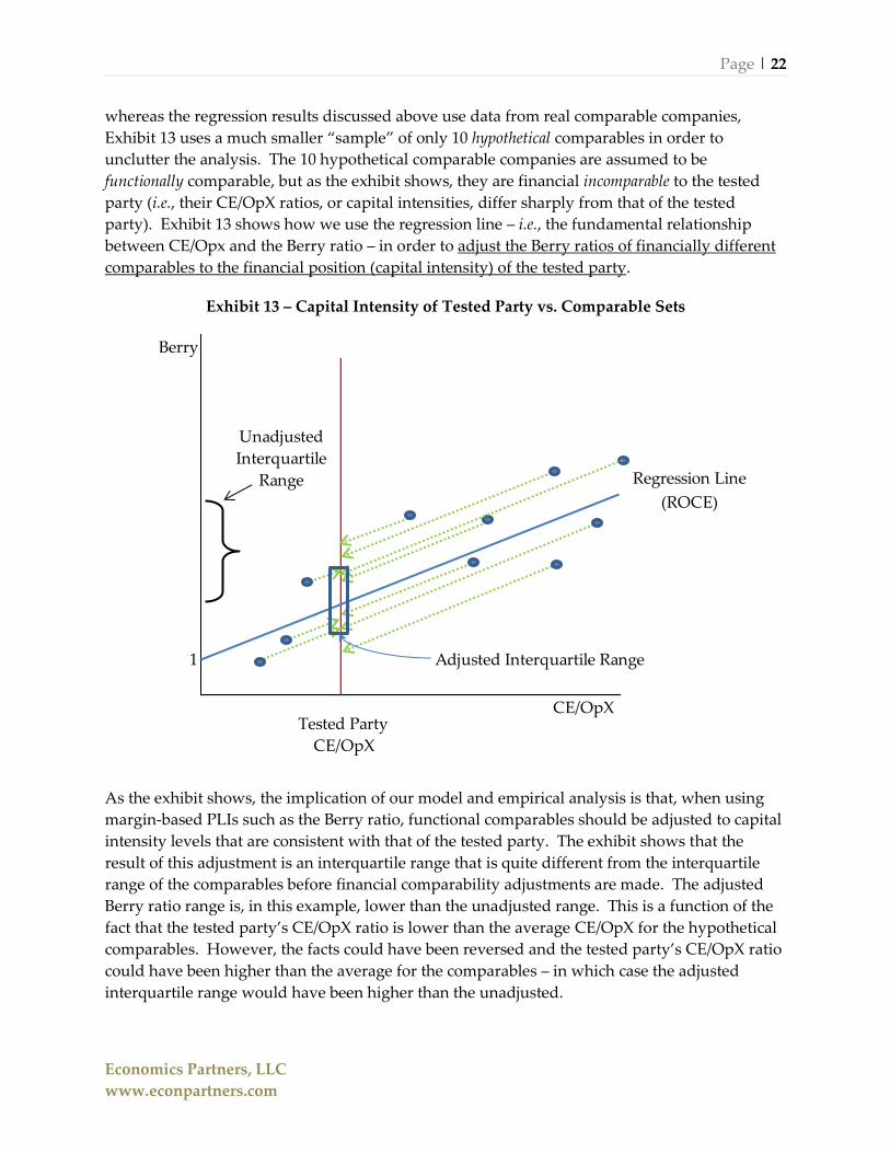
Exhibit 13, below, makes the same point, but in a slightly different manner. In addition to a

hypothetical tested party, Exhibit 13 utilizes a set of hypothetical comparables. In other words,

0.90

1.00

1.10

1.20

1.30

1.40

1.50

Capital Intensity vs. Berry Radio

Full Set

Industry Set

CE/OpX

Tested Party

Full Set

Median

Industry Set

Median

Berry

Ratio

Page | 22



whereas the regression results discussed above use data from real comparable companies,

Exhibit 13 uses a much smaller “sample” of only 10 hypothetical comparables in order to

unclutter the analysis. The 10 hypothetical comparable companies are assumed to be

functionally comparable, but as the exhibit shows, they are financial incomparable to the tested

party (i.e., their CE/OpX ratios, or capital intensities, differ sharply from that of the tested

party). Exhibit 13 shows how we use the regression line – i.e., the fundamental relationship

between CE/Opx and the Berry ratio – in order to adjust the Berry ratios of financially different

comparables to the financial position (capital intensity) of the tested party.

Exhibit 13 – Capital Intensity of Tested Party vs. Comparable Sets

As the exhibit shows, the implication of our model and empirical analysis is that, when using

margin-based PLIs such as the Berry ratio, functional comparables should be adjusted to capital

intensity levels that are consistent with that of the tested party. The exhibit shows that the

result of this adjustment is an interquartile range that is quite different from the interquartile

range of the comparables before financial comparability adjustments are made. The adjusted

Berry ratio range is, in this example, lower than the unadjusted range. This is a function of the

fact that the tested party’s CE/OpX ratio is lower than the average CE/OpX for the hypothetical

comparables. However, the facts could have been reversed and the tested party’s CE/OpX ratio

could have been higher than the average for the comparables – in which case the adjusted

interquartile range would have been higher than the unadjusted.

Berry

1 Adjusted Interquartile Range

CE/OpX

Regression Line

(ROCE)

Tested Party

CE/OpX

Unadjusted

Interquartile

Range

Page | 23



Importantly, Exhibit 13 also shows that the adjusted range is tighter than the unadjusted range.

This will always be the case. The fact that the adjustment to the comparables’ Berry ratios

involves moving them along the ROCE line toward the tested party’s CE/OpX ratio will always

increase the Berry ratios of comparables with low capital intensity, and decrease the Berry ratios

of comparables with high capital intensity. The result is a tightening of the range. This, in our

view, implies that consideration of financial comparability increases the reliability of the CPM.

B. Arm’s Length Berry Ratio Estimate Using Confidence Interval

Ranges

As noted directly above, in order to arrive at the arm’s length Berry ratio result for our routine

distributor, we simply apply the results of the regression analyses that were discussed in

Section III to the tested party. Specifically, the analysis from Section III tells us that our tested

party’s Berry ratio should be characterized by the following equation.

(6)

Therefore, we can substitute the tested party’s capital intensity ratio into the equation with the

estimates for and from the regression results to arrive at a point estimate for our routine

distributor’s Berry ratio.9

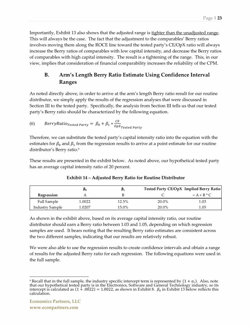
These results are presented in the exhibit below. As noted above, our hypothetical tested party

has an average capital intensity ratio of 20 percent.

Exhibit 14 – Adjusted Berry Ratio for Routine Distributor

As shown in the exhibit above, based on its average capital intensity ratio, our routine

distributor should earn a Berry ratio between 1.03 and 1.05, depending on which regression

samples are used. It bears noting that the resulting Berry ratio estimates are consistent across

the two different samples, indicating that our results are relatively robust.

We were also able to use the regression results to create confidence intervals and obtain a range

of results for the adjusted Berry ratio for each regression. The following equations were used in

the full sample.

9 Recall that in the full sample, the industry specific intercept term is represented by . Also, note that our hypothetical tested party is in the Electronics, Software and General Technology industry, so its intercept is calculated as , as shown in Exhibit 8. in Exhibit 13 below reflects this calculation.

β0 β1 Tested Party CE/OpX Implied Berry Ratio

Regression A B C = A + B * C

Full Sample 1.0022 12.5% 20.0% 1.03

Industry Sample 1.0207 15.0% 20.0% 1.05

Page | 24



(7) [ ( )]

[ ( )

]

(8) [ ( )]

[ ( )

]

Where is the industry specific fixed effect for the tested party’s industry and is

the ROCE estimate. The equation we employed to calculate this interval for the industry

comparables was similar, but it included a minor adjustment since we did not fix the general

intercept term to one. These equations are presented below.

(9) [ ( )]

[ ( )

]

(10) [ ( )]

[ ( )

]

Where is the ROCE estimate from the industry sample, and is the general intercept term

from either the industry sample. Our estimates for the upper and lower bounds of the 50

percent confidence intervals are presented below.

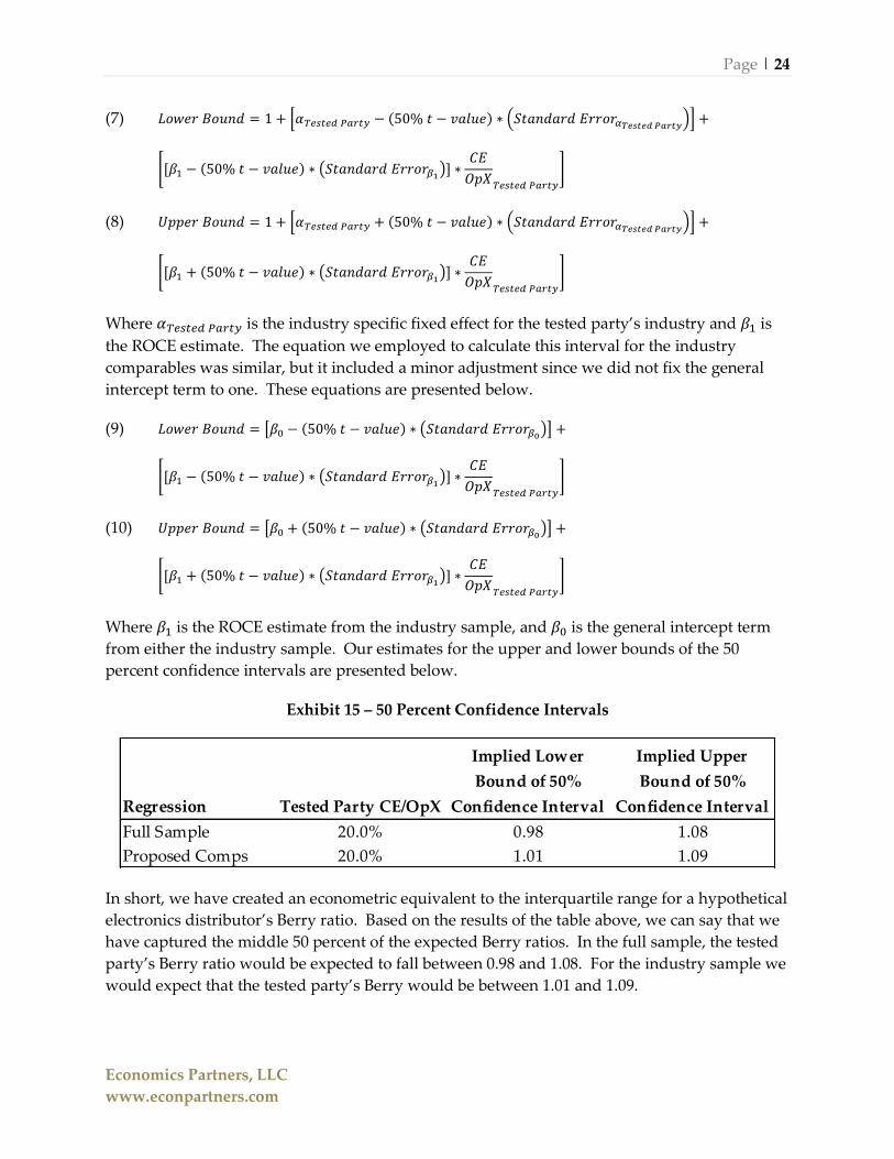
Exhibit 15 – 50 Percent Confidence Intervals

In short, we have created an econometric equivalent to the interquartile range for a hypothetical

electronics distributor’s Berry ratio. Based on the results of the table above, we can say that we

have captured the middle 50 percent of the expected Berry ratios. In the full sample, the tested

party’s Berry ratio would be expected to fall between 0.98 and 1.08. For the industry sample we

would expect that the tested party’s Berry would be between 1.01 and 1.09.

Regression Tested Party CE/OpX

Implied Lower

Bound of 50%

Confidence Interval

Implied Upper

Bound of 50%

Confidence Interval

Full Sample 20.0% 0.98 1.08

Proposed Comps 20.0% 1.01 1.09

Page | 25



V. Conclusion

We have demonstrated in this paper that the Berry ratio, along with other margin measures, can

produce unreliable results when important financial differences between the tested party and

the proposed comparable companies are ignored. Specifically, the Berry ratio that a company

earns is heavily influenced by its capital intensity ratio. More generally, margins are heavily

influenced by capital intensity, or asset turnover. Therefore, adjustments must be made in

order to account for differences in capital intensity. Such adjustments are required to ensure

financial comparability.

To illustrate this point we examined the results of a hypothetical tested party that has capital,

measured relative to value added costs, that is far lower than the capital at risk for a set of

functionally comparable distributors. While our tested party was hypothetical, the hypothetical

facts are quite consistent with facts that we see frequently in practice. We found that our

hypothetical distributor should, given the comparables’ relationship between capital employed

intensity and Berry ratio, earn a Berry ratio that is lower than the average and median Berry

ratios observed for comparable companies with higher capital intensity ratios.

Page | A-1



Appendix A: Searches for Routine Distributors

CapitalIQ™ was used to conduct these searches. CapitalIQ™ is a web and Excel-based research

platform with data on over 60,000 public companies, worldwide, obtained directly from public

filings. Screens can be conducted using over 400 qualitative items and 900 quantitative items,

and direct links to the public filings are provided through the CapitalIQ™ software.

1. Search Process – Full Sample

a) Industry Classification

CapitalIQ™ employs the Standard Industrial Classification (“SIC”) system. A review and

comparison of functions performed by the tested party to functions and activities listed in the

SIC system allowed us to narrow the search to the following industry classifications:

1) 5000: Durable good - wholesale

2) 5010: Nondurable goods - wholesale

Companies classified under these SIC codes are most likely to be similar to a routine distributor

in terms of functions performed, assets employed, risks assumed, and business conditions

faced. After applying this filter, 291,745 companies remained.

b) Ownership and Operating Status

In order to further narrow our sample, additional filters were added to include only publicly

traded companies, private companies with public issued debt, and currently operating

companies or subsidiaries.

After applying this filter, 1761 companies remained.

c) Geographic Filter

We narrowed the results to include US companies. This search filter resulted in 361 companies.

d) Insufficient Financial Data

We then examined the financial data of the remaining set of 361 potentially comparable

companies. We eliminated any firms with either missing or incomplete financial data. After

this filter was applied, 159 firms remained in our sample.

2. Search Process – Industry Sample

a) Industry Classification

For our computer and electronics industry set, we narrowed the search to the following

industry classifications:

Page | A-2



1) 5045: Computers, Peripherals, and Software

2) 5060: Electrical Goods – Wholesale10

This initial search filter resulted in 29,683 potential comparables.

b) Ownership and Operating Status

In order to further narrow the initial results, additional filters were added to include only

publicly traded companies and currently operating companies or subsidiaries.

After applying this filter, 931 potential comparables remained.

c) Geographic Filter

We further narrowed the results to include those companies operating in the U.S. or Canada.

This search filter resulted in 90 potentially comparable companies.

d) Quantitative Screening Filters

We reviewed the financial data for the potential comparables, and performed a series of

quantitative screening procedures. Quantitative screening eliminates potential comparables

based on balance sheet or income statement figures or ratios that are known to be indicative of

significant differences in functions, assets, or risks. In this stage of the screening process, we also

eliminated potential comparables for which we have an insufficient number of years of publicly

available financial data to allow for a reliable comparison with the tested party.

(1) Negative Operating Earnings

Companies with negative operating income are generally not considered comparable because

their financial results may reflect idiosyncratic market impacts or actions taken by management

in direct response to their financial instability. In order to eliminate these companies we added

an additional screen to ensure that the companies had at least one year of positive operating

earnings over the previous three years. We also excluded any company with no reported

financials over the most recent five year period. This screen resulted in the elimination of ten

companies.

(2) Net Revenue

We eliminated companies whose five-year average net sales were less than $50 million.

Significant differences in size between comparables and the tested party may indicate the

presence or absence of economies of scale or scope, which in turn suggest significant differences

in functions and risks. This screen resulted in the elimination of thirty-six companies.

10 SIC Code 5060 includes 5063 (Electrical apparatus and equipment), 5064 (Electrical appliances, televisions and radios), and 5065 (Electronic parts and equipment not elsewhere classified).

Page | A-3



(3) Property, Plant & Equipment (“PP&E”) to Sales

Next, we screened for companies whose five-year weighted average ratio of net property, plant,

and equipment ("PP&E") to net sales was greater than 15 percent. The existence of significant

amounts of PP&E can be indicative of either manufacturing activities or, in the case of a

distributor, of investment in warehouses, material handling equipment, and other assets

necessary to handle a large inventory. In either case, there are likely to be significant differences

in functions and risks between companies that have substantial investment in PP&E and those

that do not. This screen resulted in the elimination of three companies.

(4) Research & Development Expense to Sales

We screened for companies whose five-year average ratio of research and development expense

to net sales was greater than three percent. Companies who engage in significant research and

development activities often own significant technology-related intangibles. The development

and ownership of intangibles leads to significant differences in functions and risks between

companies that engage in these research and development activities and those that do not. A

routine distributor typically does not engage in research and development activities nor does it

own any significantly valuable intangibles. This screen resulted in the elimination of two

companies.

(5) Sales and Marketing Expense to Sales

We next screened for companies whose five-year weighted average ratio of sales and marketing

expense to net sales was greater than three percent. Companies that engage in substantial sales

and marketing activities may own significant marketing-related intangibles such as trademarks

or brand equity. As a result, there are likely to be significant differences in functions and risks

between companies that incur significant advertising expenses and those that do not. This

screen resulted in the elimination of one companies.

The results of these quantitative screening filters resulted in the elimination of 52 companies,

leaving 38 potentially comparable companies.

e) Qualitative Review

In our qualitative assessment, we reviewed the business descriptions, as provided by the

database, investor relations material, and websites, when available.

Through this process, it was determined that 26 of the 38 companies reviewed were engaged in

activities that are insufficiently comparable to those of routine computer and electronics

distributor. We eliminated companies with obviously unrelated operations, companies

distributing insufficiently comparable products, and companies with insufficient information to

determine comparability.

Page | A-4



Our search process resulted in the 12 comparable companies listed below that we considered

sufficiently similar in terms of business operations, assets employed and risks assumed.

1. Alliance Distributors Holding Inc.

2. Avnet Inc.

3. Brightpoint Inc.

4. GTSI Corp.

5. Ingram Micro Inc.

6. Insight Enterprises Inc.

7. Navarre Corp.

8. ScanSource, Inc.

9. SED International Holdings, Inc.

10. Softchoice Corp.

11. SYNNEX Corp.

12. Tech Data Corp.

economics partners, llc white paper · pdf fileeconomics partners, llc white paper series tim...

Documents