economics of forest landscape restoration
TRANSCRIPT

Economics of Forest Landscape RestorationEstimating impacts, costs and benefits from ecosystem services

Economics of Forest Landscape RestorationEstimating impacts, costs and benefits from ecosystem services
Client acknowledgementThis study is supported by the GIZ International Forest Program (IWP) with funds from the Ger-man Federal Ministry for Economic Cooperation and Development (BMZ). Its main purpose iscontributing to the successful achievement of global and national FLR targets, in particular theAFR100 initiative, which promotes FLR in Sub-Saharan Africa.
AuthorsDuncan Gromko, Till Pistorius, Matthias Seebauer, Andrea Braun, Eva Meier
Date: 15 October 2019

UNIQUE | Economics of FLR iii
TABLE OF CONTENTS
List of tables ..................................................................................................................................ivList of figures .................................................................................................................................ivList of abbreviations .......................................................................................................................v
Preface .......................................................................................................................................... 7Executive Summary....................................................................................................................... 81 Introduction ........................................................................................................................... 102 Overview of methodology ..................................................................................................... 123 Process for the analysis.......................................................................................................... 15
3.1 Step 1: Set the scene ...................................................................................................... 15
3.2 Step 2: Model costs and benefits ................................................................................... 23
3.3 Step 3: Data collection ................................................................................................... 39
3.4 Step 4: Analysis of costs and benefits ............................................................................ 41
4 Conclusions ............................................................................................................................ 455 Literature and Sources ........................................................................................................... 47
Annex 1: Glossary of terms ......................................................................................................... 50Annex 2: Ecosystem service modeling tools ............................................................................... 53Annex 3: Approach for Estimating biodiversity values ............................................................... 56

UNIQUE | Economics of FLR iv
LIST OF TABLESTable 1: Examples of FLR options................................................................................................ 17Table 2: Stakeholder types.......................................................................................................... 18Table 3: Differences between financial and economic analyses ................................................ 19Table 4: Overview of different ecosystem services categories................................................... 20Table 5: Example summary of costs and benefits by beneficiary type (US$, per ha) ................. 24Table 6: Valuation methodologies adapted from (Verdone, 2015) ............................................ 27Table 7: GHG effects of common types of FLR activities ............................................................ 28Table 8: Runoff curve number method....................................................................................... 34Table 9: Runoff Coefficient.......................................................................................................... 34Table 10: Example of qualitative employment impacts.............................................................. 36Table 11: Generalized costs and benefits for FLR activity types per hectare (US$).................... 40Table 12: Simplified net values model (US$)............................................................................... 41Table 13: Example sensitivity table (IRR) .................................................................................... 44Table 14: Ecosystem service modeling tools; table is largely taken from (WRI; IUCN, 2014), with
some additions and alterations .............................................................................. 53
LIST OF FIGURESFigure 1: ROAM methodology (WRI; IUCN, 2014) ...................................................................... 12Figure 2: Overview of methodology............................................................................................ 13Figure 3: Example key questions................................................................................................. 15Figure 4: Three tiers of analysis, based upon quality of input data............................................ 16Figure 5: Scenario example ......................................................................................................... 22Figure 6: Moving between modeling and data collection .......................................................... 23Figure 7: Step by step approach for quantifying GHG emission reductions ............................... 29Figure 8: Context modules to calibrate the tool to location conditions of the FLR activity ....... 30Figure 9: Selection chart of EX-ACT land use modules based on the specific FLR activity types 30Figure 10: Overview of calculation to measure soil loss change ................................................ 32Figure 11: Step-wise approach for biodiversity assessment....................................................... 38Figure 12: Example Monte Carlo analysis ................................................................................... 44Figure 13: Matrix for biodiversity risk assessment when implementing business models......... 57Figure 14: Tourism case study..................................................................................................... 58

UNIQUE | Economics of FLR v
LIST OF ABBREVIATIONSA/R Afforestation / Reforestation
AFOLU
AFR100
Agriculture, Forestry and other Land Uses
African Forest Landscape Restoration Initiative
ANR Assisted Natural Regeneration
CO2e Carbon dioxide equivalent
ELD Economics of Land Degradation
FAO Food and Agriculture Organization of the United Nations
FCPF Forest Carbon Partnership Facility
FLR Forest Landscape Restoration
FRA Forest Resource Assessment (FAO)
FSC Forest Stewardship Council
FTE Full time equivalent
GCF Green Climate Fund
GDP Gross Domestic Product
GHG Greenhouse Gas Emissions
GIS Geographic Information Systems
GIZ Deutsche Gesellschaft für Internationale Zusammenarbeit
GPFLR Global Partnership on Forest Landscape Restoration
Ha hectareIFC International Finance Corporation
IPBESIntergovernmental Science-Policy Platform on Biodiversity and EcosystemServices
IRR Internal Rate of Return
IUCN International Union for Conservation of Nature
IUFRO International Union of Forest Research Organizations
LDD Land degradation and desertification
LDN Land Degradation Neutrality
M&E Monitoring and Evaluation
MDG Millennium Development Goals
NDC Nationally Determined Contribution
NGO Non-Governmental Organization

UNIQUE | Economics of FLR vi
NPV Net Present Value
NTFP Non-Timber Forest Product
NYDF New York Declaration on Forests
ODA Official Development Assistance
ROAM Restoration Opportunities Assessment Methodology
ROE Return on Equity
ROI Return on Investment
RUSLE Revised Universal Soil Loss Equation
SALM Sustainable Agriculture Land Management
SDG Sustainable Development Goals
SER Society for Ecological Restoration
SFM Sustainable Forest Management
SLM Sustainable Land Management
TAV Total Available Water
TEV Total Economic Value
UNCCD United Nations Convention to Combat Desertification
UNFCCC United Nations Framework Convention on Climate Change
USLE Universal Soil Loss Equation
WACC Weighted Average Cost of Capital
WRI World Resources Institute

PREFACEImagine you are a cocoa farmer in Ghana, a cattle rancher in Paraguay, or a dairy farmer in theNetherlands. Your family’s livelihood – the school fees of your children, your mother’s hospitalcosts, and your food and shelter – all depend on the income that you make from your land. Thefarm succeeds when the soil has sufficient nutrients, the spring is flowing, the climate is favora-ble, and you can afford the time and money to manage every aspect of the farm just right. If thisbalance is off, the farm and your family will be worse off.Even more than the food and income that the farm provides you, living on the farm is central toyour quality of life. You have never been attracted by the hectic life of large cities and the airpollution – you appreciate the clean air and water you have access to in the countryside. Yourpartner wakes up early every morning to watch the birds and your children play in the farm afterschool. What’s more, you take pride in growing food and preserving the traditional farmer life.Farm life is not romantic: it is arduous and full of risks. About third of your farm is underper-forming. Your parents faced tough times when you were young and cleared a large area of trees,initially to sell the wood and subsequently to plant with a new crop, which did not do well andsucked the nutrients from the soil. The spring gives less water than before and there seem to befewer birds and insects.You have heard that neighbors are facing similar difficulties and realize you have to change yourpractices. After saving for a few years, you and your family now have enough money to invest inthe land. What should you do? You could buy a tractor, seeds, and fertilizer, allowing you tointensify and expand your farming operations on the land. Your partner prefers to replant nativetrees there, so that more birds will come to your land. You are also tempted to try a new agro-forestry system similar to what your neighbor has started. How do you choose between thesedifferent options and the benefits to your family?These are the choices that farmers, land managers, and policy makers around the world arefacing. An estimated 2 billion hectares of the world’s forests and natural ecosystems are de-graded, hurting agricultural productivity and diminishing the clean air, water, and other vitalservices these ecosystems provide. If we invest into restoring degraded lands, what ecosystemservices do we prioritize? How can we compare the value of producing more agricultural goods,regulating our global climate, creating jobs, or protecting biodiversity? There are some restora-tion options that provide “win-wins”. However, in many cases there are short and long-termtradeoffs between different land management options and decisions.The aim of the toolbox described in this report is to aid in this decision-making, for the farmerin Ghana, Paraguay, or the Netherlands, as well as large agribusinesses or local and regionalgovernments that envision largescale restoration programs at a landscape scale. It recommendsa straightforward, four-step process and provides guidelines and tools for each step. Assessingthe costs and benefits of land use investments will allow decision-makers to prioritize restora-tion investments based on criteria that matter to them: which ecosystem services are prioritized,who should benefit, and when are benefits realized. By projecting the quantities of ecosystemservices produced under different investment scenarios – and putting a monetary value on thoseservices when helpful – we can understand the tradeoffs between scenarios and make decisionsto optimize land use.
UNIQUE | Economics of FLR 8
EXECUTIVE SUMMARYThe Bonn Challenge, the New York Declaration on Forests (NYDF, 2014), and regional initiativeshave created unprecedented momentum for reversing land and forest degradation. The globalarea that could be restored is estimated up to 2 billion hectares, and with the unabated pressureon forests, this figure continues to grow. Restoration at scale is thus an imperative to achievingthe sustainable development goals (SDGs) and other internationally agreed policy objectives.These initiatives have successfully promoted and triggered massive political commitment for theconcept of Forest Landscape Restoration (FLR). Many countries have made ambitious restora-tion pledges. They often consider restoration as a key strategy under their Nationally Deter-mined Contributions to the UNFCCC Paris Agreement.Today, FLR is a globally known approach for aligning national “green economy” developmentagendas and sustainable management of natural resources. Despite the benefits, one barrier toimplementing FLR at scale is the significant costs associated with many FLR activities. Conse-quently, attracting sufficient funding continues to be one of the key challenges: it is estimatedthat US$36 to 49 billion are needed annually in order to reach Bonn Challenge and NYDF resto-ration goals, respectively (FAO & UNCCD, 2015). While funds that target FLR investments havebeen developed, the scale of investment being deployed is nowhere near what is required.The diverse set of benefits generated by FLR investments – from increased agricultural yields, toglobal climate change mitigation, to improved soil and water regulation – is an important reasonfor the interest in FLR. Convincing and comprehensive cost-benefit analyses can be a powerfultool for FLR advocates – policy makers and potential investors – to raise interest and createdemand for FLR. The challenge lies in estimating a value of the benefits that is relevant to thestakeholders that are involved in decision-making.Against these considerations, this report “Economics of Forest and Landscape Restoration” hasdeveloped an easily applicable economic framework, helping stakeholders to develop a custom-ized decision-making tool. Consisting of standalone modules and methods, it offers both privateand public actors differentiated means of estimating values. Tailored cost-benefit analyses canhelp a variety of different target groups in their decision-making: from farmers and agribusi-nesses to local and national level governments.Assessing the costs and benefits of land use investments will allow decision-makers to demon-strate that investments in FLR are worth the short-term cost for public entities and result inbetter economic and environmental outcomes. The modeling and its results furthermore allowfor prioritizing restoration investments based on different criteria: which ecosystem services areprioritized, who should benefit, and when will benefits be realized? Does the farmer choose toimprove agricultural productivity, to protect water resources, to avoid erosion, or some combi-nation? Policy makers need to understand the costs of FLR as well as the multiple benefits: em-ployment effects, tax and Gross Domestic Product (GDP) contribution, and indirect economicvalues – for example, the value of carbon sequestration and non-marketable ecosystem servicesas avoided erosion and hydrological services.The framework at hand consists of a straightforward, four-step process. It provides guidelinesand tools for each step: setting the scene, data collection, modeling costs and benefits, andanalysis of results. The methodology is applicable for users with different needs and access to

UNIQUE | Economics of FLR 9
resources. Both low- and high-cost assessments are possible, depending on the purpose of theanalysis and the level of complexity needed.The methodology complements ROAM and other restoration opportunity tools, e.g. by provid-ing a cost-benefit analysis of the opportunities identified during a preliminary assessment. It canbe applied as part of a restoration opportunity process, once FLR activities have been identifiedand mapped, but also as a stand-alone decision making tool. The results will allow decision-makers to compare the trade-offs between alternative FLR investment scenarios, and to informdecision processes and land use planning.

UNIQUE | Economics of FLR 10
1 INTRODUCTIONUnabated deforestation and forest degradation have led to vast areas of degraded lands andforests around the world. Land degradation is the consequence of different land use interven-tions that are often aggravated by natural responses, e.g. erosion, desertification, or invasivespecies (Gibbs & Salmon, 2015). Despite many initiatives at different levels, ongoing land andforest degradation remain drivers of food insecurity, climate change, and biodiversity loss (IPCC,2007b, 2007a; Pan et al., 2011; Pereira et al., 2010; Wreford, Moran, & Adger, 2010). Land deg-radation occurs when the different ecological processes of ecosystems are disrupted by changesinduced directly or indirectly by humans. With the decline in their ecological functions, degra-dation means that land is not as productive as in its pre-disturbance state: it provides less prod-ucts and ecosystem services. Globally up to 2 billion hectares (ha) are degraded and could berestored (Bonn Challenge, 2018; WRI, 2011).Reducing and reversing degradation will help achieve international environmental and devel-opment objectives. Restoring degraded lands could be a win for global livelihoods, particularlyfor people living in rural areas, as it would improve agricultural incomes and other ecosystemservices. Since 2010, a number of international policy agreements have established a frameworkto achieve the promise of land restoration. The most important are the 2010 Aichi Targets ofthe Convention on Biological Diversity (CBD), the Land Degradation Neutrality Target under theUnited Nations Framework Convention on Combating Desertification (UNCCD), and the 2015Paris Agreement under the United Nations Framework Convention on Combating ClimateChange (UNFCCC). Besides these processes, the United Nations Declaration on Forests of 2014,high-level policy dialogues as the Bonn Challenge and its related initiatives and the SustainableDevelopment Goals (SDGs) of 2015 have formulated objectives related to restoring forest land-scapes. Moreover, many national-level climate change, forestry, and land use policies and strat-egies include land restoration targets and objectives.The Bonn Challenge, the follow-up process on the New York Declaration on Forests (NYDF),AFR100, and the 20*20 initiative – are fostering implementation on the ground. Their explicitrationale is to promote the concept, encourage countries to make voluntary FLR pledges, and tofoster and upscale FLR measures. As of August 2019, 59 governments have pledged to restoremore than 170 million ha; often the pledges are linked to formal national and international pol-icy targets, such as the Nationally Determined Contributions (NDCs) under the Paris Agreement.The concept of FLR aligns with national “green economy” agendas and sustainably managingnatural resources. FLR has a strong focus on the benefits that restored ecosystems can provideto humans. Following the currently produced Intergovernmental Science-Policy Platform on Bi-odiversity and Ecosystem Services (IPBES) thematic assessment on land degradation,1 this doc-ument uses the following definition of restoration: “any intentional activity that initiates or ac-celerates the recovery of an ecosystem from a degraded state.” This understanding embraces
1 Report available at: https://www.ipbes.net/system/tdf/ipbes_6_inf_1_rev.1_2.pdf?file=1&type=node&id=16514

UNIQUE | Economics of FLR 11
the economic monetary and non-monetary values that ecosystems provide for the well-beingand livelihoods of mankind.2
Attracting sufficient funding for FLR investments is a key challenge for successful implemen-tation. While countries have set restoration goals, achieving these targets will require unprece-dented financial and political commitment to FLR; US$36 – 49 billion are needed annually inorder to reach Bonn Challenge and NYDF restoration goals, respectively (FAO & UNCCD, 2015).FLR advocates need to make the economic case that investments in FLR are worth the short-term cost for public entities and result in better outcomes. Policy support is needed enable FLR– improving governance, legal frameworks, providing financial incentives, and enhance land useplanning. For coping with these challenges policy makers need to understand the costs of FLR aswell as the multiple benefits. They include employment effects, tax and Gross Domestic Product(GDP) contribution, and indirect economic values – for example, the value of carbon sequestra-tion or avoided erosion.The success of the approach will rely on attracting significant private sector engagement andinvestment. Some financial institutions have made commitments to invest in restoration; forexample, investors have earmarked US$ 2 billion for restoration investments in Latin America.3
However, these funds are insufficient to meet the challenge at hand. Moreover, these fundshave not been fully deployed. FLR has not captured the attention of private sector and otherlarge-scale institutional investors in any significant way. One important step to convincing pri-vate sector actors to invest in FLR is to demonstrate that FLR business models can generatereturns and be financially viable.Policy makers and private sector actors have different information needs about values gener-ated by single FLR investments, multi-activity programs, and implementation at landscapelevel. Private sector actors are primarily interested in understanding the financial implicationsof specific investments: investment needs, expected cash flows, profitability expectations, andrisks. In many sectors, particularly agriculture, forestry, and hydropower, the return expecta-tions are directly related to ecosystem function and the flow of ecosystem services. Policy mak-ers may be more interested in the macro-economic impacts of FLR, such as primary and second-ary employment, tax generation, GDP contribution, and revenue creation for specific sectors.Credibly estimating, quantifying, and, in some cases, monetizing the multiple impacts of FLR canbe an important tool for communicating its value to public and private sector actors.The main purpose of this study is to develop a practical methodology that enables a rapid,realistic, and robust estimation of the economic impacts of FLR. It will inform investors andpolicy makers based on their actual information needs, as well as development professionalsworking in the fields of forestry, agriculture, and climate resilience. Cost-benefit analysis as adecision-making tool is well understood, but the report should help fully account for the benefitsof FLR and communicate them to a broader audience.
2 In a rigorous academic interpretation the correct term would be ‚rehabilitation‘. However, the authors of this reportshare the broad view that the synonymous use in policy discourses reflects the reality that restoration is a long processwith uncertain outcomes.3 For more information on investor commitments, see: https://www.wri.org/our-work/project/initiative-20x20/im-pact-investors#project-tabs
UNIQUE | Economics of FLR 12
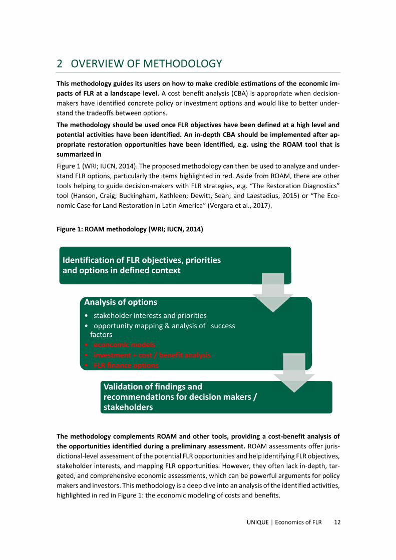
2 OVERVIEW OF METHODOLOGYThis methodology guides its users on how to make credible estimations of the economic im-pacts of FLR at a landscape level. A cost benefit analysis (CBA) is appropriate when decision-makers have identified concrete policy or investment options and would like to better under-stand the tradeoffs between options.The methodology should be used once FLR objectives have been defined at a high level andpotential activities have been identified. An in-depth CBA should be implemented after ap-propriate restoration opportunities have been identified, e.g. using the ROAM tool that issummarized inFigure 1 (WRI; IUCN, 2014). The proposed methodology can then be used to analyze and under-stand FLR options, particularly the items highlighted in red. Aside from ROAM, there are othertools helping to guide decision-makers with FLR strategies, e.g. “The Restoration Diagnostics”tool (Hanson, Craig; Buckingham, Kathleen; Dewitt, Sean; and Laestadius, 2015) or “The Eco-nomic Case for Land Restoration in Latin America” (Vergara et al., 2017).
Figure 1: ROAM methodology (WRI; IUCN, 2014)
The methodology complements ROAM and other tools, providing a cost-benefit analysis ofthe opportunities identified during a preliminary assessment. ROAM assessments offer juris-dictional-level assessment of the potential FLR opportunities and help identifying FLR objectives,stakeholder interests, and mapping FLR opportunities. However, they often lack in-depth, tar-geted, and comprehensive economic assessments, which can be powerful arguments for policymakers and investors. This methodology is a deep dive into an analysis of the identified activities,highlighted in red in Figure 1: the economic modeling of costs and benefits.
Identification of FLR objectives, prioritiesand options in defined context
Analysis of options• stakeholder interests and priorities• opportunity mapping & analysis of success
factors• econcomic models• investment + cost / benefit analysis• FLR finance options
Validation of findings andrecommendations for decision makers /stakeholders

UNIQUE | Economics of FLR 13
The methodology is applicable for users with different needs and access to resources. Bothlow and high-cost assessments are possible, depending on the purpose of the analysis and thelevel of complexity needed. The authors distinguish between three tiers: A Tier 1 analysis is based on simple methods, proxies, default values and benchmarks. It
results in estimations that should be conservative and robust. The assessment requiresrelatively little time for data collection, but does not deliver results that the user shouldhave high confidence in; Tier 1 analysis is most appropriate at an early scoping stage.
Tier 2 analysis refines the estimation and uses empirically backed national or even localdata and benchmarks. It may incorporate some primary data collection and can be usedas a basis for investment decisions.
Tier 3 analysis incorporates spatially explicit high-resolution activity data and analysis.This level of detail becomes appropriate the impacts of potential activities dependgreatly on the spatial distribution in a given landscape. This level of analysis requiressignificantly greater time and resource input.
Having decided upon the appropriate tier, the user should then follow the step-wise approachsummarized in Figure 2.
Figure 2: Overview of methodology
Step 1 helps to set the parameters of the analysis. The user should start by listing the primaryquestions that should be answered by measuring costs and benefits. FLR activities should be
Set the Scene
•Define key questions•Finalize FLR activities•Map beneficiaries•Which benefits are measured and from whose perspective•Define scenarios
Model Costsand Benefits
•Costs•Provisioning services•Regulating and cultural services•Other benefits•Spatial analysis (optional)
DataCollection
•Identify data needs•Collect field data•Gather benchmark data•Refine methodologies
AnalyzeResults
•Analyze results using different indicators•Account for uncertainty

UNIQUE | Economics of FLR 14
defined, end beneficiaries need to be mapped, and the user should decide which ecosystemservices will be included. Based upon all of this, scenarios are developed.Step 2 (Model Costs and Benefits) and Step 3 (Data Collection) are separate, but will likelyrequire an iterative process of moving back and forth to refine and improve results. The pro-cess of monetizing ecosystem services is broken down into a simple equation: Value = Price *Quantity. Values of ecosystem services are modeled over time, estimated at regular time inter-vals. Both primary data and benchmark data can be collected. It is likely that data gaps may stillremain after a first round of data collection, necessitating the user to possibly refine his or hermethodologies or seek new sources. The results help stakeholders, policy makers, and investorsto understand what investments are required and their expected impacts.Step 4 finalizes the analysis by interpreting the results. Different financial and economic indi-cators can help to communicate the impact of results to different stakeholders. Additionally,uncertainty can be high in cost benefit analysis and tools like a sensitivity analysis can help toaccount for this.

UNIQUE | Economics of FLR 15
3 PROCESS FOR THE ANALYSIS
3.1 Step 1: Set the sceneUnder Step 1 users establish the parameters of their analysis. They have to be clear about thepurpose of the analysis, what activities are relevant, who is involved, and what is being meas-ured. Key questions for the analysis should be established at this time in order to ensure thatthe outputs of the analysis are helpful. Relevant stakeholders should be identified and FLR ac-tivities to be evaluated should be finalized. Development of scenarios will allow the user to com-pare the baseline scenario to alternative investment or policy scenarios. Determining what ben-efits are measured and which actors are included will have a large impact on the scope andextent of the analysis.
Determine key questionsThe first step in setting the scene is to clearly lay out the parameters of the analysis and iden-tify the key questions. See Figure 3 for typical questions that a cost-benefit analysis can help toaddress.Figure 3: Example key questions
What are the costs of inaction? What will happen if we continue under business as usual? What investments or policies produce the greatest benefits? What are the costs? Which considerations cannot be quantified or monetized, and thus are not included in a cost-ben-
efit analysis? What resources are available to conduct an analysis and what level of confidence is needed at this
point? What are the total environmental / social / financial benefits of different investment scenarios? Which investment scenarios are most profitable? Which are most cost-effective? By how much do different groups / individuals benefit under different scenarios? How much do
different groups / individuals lose under different scenarios? Which scenarios are most effective in leveraging public investment? What are key risks / threats to a potential FLR investment? What are the total costs of different scenarios?
One key question to highlight is the need to determine the appropriate level of complexity.On the one hand, a complex analysis that collects significant primary data will give the user ahigher degree of confidence in the results. On the other hand, increasing complexity raises thecosts of the analysis itself, and may not be necessary at an early stage of decision-making. Thelevel of complexity of analyses can be broadly categorized into three tiers (Figure 4). It is up tothe user to determine the tradeoffs between the desire for accuracy and costs.In Tier 1 and 2 analyses, the user will generate a one-hectare model for each activity includedin the cost-benefit analysis. These one-hectare models are then scaled-up across the entire areaof the proposed project. It is important to note the limitations of using one-hectare models. Theecological functions, the ecosystem services it provides and the overall productivity of one hec-tare of land is greatly affected by surrounding areas. A one hectare FLR investment will likely nothave the same per hectare productivity as a thousand-hectare investment. Tier 3 analyses may

UNIQUE | Economics of FLR 16
develop spatially explicit models, meaning that costs and benefits may vary by geography, andhomogenous one-hectare models will not be used.One option for managing these tradeoffs is to do two stages of analyses. A first stage analysiswould rely primarily on readily-available benchmark data and would be less costly. If the resultsare promising, the user may decide to continue with a second stage analysis, investing more indata collection and following a tier two or three approach.
Figure 4: Three tiers of analysis, based upon quality of input data
Identify FLR activitiesThis methodology can be applied on its own, or as a partof a broader decision-making process. ROAM assess-ments, for instance, have identified potential FLR activitiesand their suitability within the target country or landscape.Key opportunities identified by a ROAM should be chosenfor a full cost and benefit analysis. For example, theRwanda ROAM identified five potential FLR interventions(Rwanda, 2016): agroforestry on steep sloping land combined with
soil conservation measures, agroforestry on gently sloping land, improved management of woodlots and planta-
tions, protection and restoration of existing natural forests, establishment or improvement of protective areas on important and sensitive sites.
Generally, FLR activities can be categorized as described in Table 1, based on the current useof land; specific FLR actions that may fall in more than one category.
Tier 1
• Low cost• Reliant primarily onreadily-available,benchmark data; primarysources used
• Appropriate at a pre-feasibility stage
• Likely not rigourousenough to makeinvestment planningdecisions
Tier 2
• Low cost if country-specific data is available
• A mix of benchmarkdata and primarysources; little or no useof spatially-explicit data
• Can support investmentplanning decisions
• Appropriate whenpriority ecosystemservicesare not spatially-dependent
Tier 3
• High cost• Highly reliant onprimary data; significantincorporation ofspatially-explicit data
• Can support investmentplanning decisions
• Appropriate whenpriority ecosystemservices are spatially-dependent

UNIQUE | Economics of FLR 17
Table 1: Examples of FLR options
Land use Land sub-type FLR option Description
Forest land
Land where forestis, or planned tobecome the domi-nant land use
Suitable forwide-scalerestoration
Forest land iswithout trees
(temporarilyunstocked)
Planted for-ests & wood-lots
Planting of trees on formerly forested land. Na-tive species or exotics and for various purposes,fuelwood, timber, poles, fruit production, etc.
Natural
regeneration
Natural regeneration of formerly forested land. Ifthe site is heavily degraded and no longer hasseed sources, planting will be required
Degradedforests
Silviculture /sustainableforest man-agement
Enhancement of existing forests and woodlandsof diminished quality and stocking, e.g. by manag-ing pressures (fire, grazing) & silvicultural inter-ventions
Agricultural land
Land which is be-ing managed toproduce food
Suitable formosaic resto-ration
Land is underpermanentmanage-ment:
Agroforestry
Establishment & management of trees on agricul-tural or pasture land (planting or regeneration),to improve crop productivity, provide dry seasonfodder, increase soil fertility, enhance water re-tention, etc.; includes silvopastoral systems
Integratedsoil fertilitymanagement
Soil regenerative practices, such as no-till farming,planting of cover crops during fallow periods,planting nitrogen-fixing species, use of fertilizer,etc.
Land is underintermittentmanage-ment:
Improvedfallow
Establishment and management of trees on fal-low agricultural land to improve productivity, e.g.by fire control, extending the fallow period etc.,
Protective landand buffers
Land vulnerableor critical in safe-guarding
Suitable formangroverestoration,watershedprotectionand erosioncontrol
If degradedmangrove:
Mangrove
restorationEstablishment or enhancement of mangrovesalong coastal areas and in estuaries
If other pro-tective landor buffer:
Watershedprotectionand erosioncontrol
Establishment and enhancement of forests onvery steep sloping land, along water courses, inareas that naturally flood and around critical wa-ter bodies
Source: Adapted from IUCN & WRI (2014), page 39
Appropriate FLR activities are always context-specific; an activity that is considered to be re-storative in one geography may not be FLR in different contexts. The level of degradation, cur-rent economic activities, biophysical factors, and other factors will determine which FLR activi-ties are appropriate. If a ROAM assessment has been completed, it will have analyzed the suita-bility of different FLR activities in the target geography. If a ROAM assessment has not beencompleted, the user should ensure that activities are technically feasible in the proposed areas.

UNIQUE | Economics of FLR 18
Map beneficiaries and other stakeholdersAs a next step, beneficiaries and other stakeholdersshould be mapped. Stakeholder mapping is an im-portant part of any decision-making process, but ithas a specific purpose in determining the costs andbenefits of an FLR investment: it is critical to definestakeholders by the costs that they assume and thebenefits that accrue to them.Table 2 describes potential stakeholders, and the rele-vant costs and benefits.
Table 2: Stakeholder typesStakeholder type Potential costs Potential benefitsPublic sector Directly purchase, lease, or sub-
sidize land, materials, equip-ment, and labor Fiscal incentives for improved
land use or commodity pro-duced
Increased tax collection Political support
Land owners or pri-vate sector compa-nies
Purchase or lease land, materi-als, equipment, and labor Opportunity cost of current
land use
Increased production and/or prices Improved local ecosystem services un-
related to production Reputational benefits
Community membersnot owning land
Opportunity cost of currentland use Labor
Employment opportunities Higher supply of forest or agricultural
products Improved local ecosystem services un-
related to production
Commodity offtakers Price premium or other subsidyfor commodities produced un-der FLR system
Improved access to supply Price premium from own customers Reputational benefits
Global / regionalcommunity
Taxes contributing to FLR in-vestment
Climate change mitigation Improved water management, re-
duced soil erosion, or ES that benefitpeople outside of the project area Biodiversity benefits

UNIQUE | Economics of FLR 19
Which benefits are measured and from whose perspectiveNext, the user should decide on the perspec-tive of the analysis and the costs and benefitsto be measured, and the benefits that shouldbe included. A cost-benefit analysis can bedone from the perspective of any number of ac-tors: a private investor, a community, a politicaljurisdiction, a country, or even the global com-munity.A financial analysis takes a narrow perspectivethan an economic analysis, i.e. typically a private sector entity implementing the investment.Table 3 summarizes the differences between financial and economic analysis. Costs and benefitsare restricted to the financial flows that actually materialize, such as upfront and managementcosts, increased revenues from products sold, and any fiscal incentives from the public sector.Benefits from ecosystem services can be included in a financial analysis, but only those thatwill affect the cash flows of the business, e.g. reduction in soil erosion that lead to improvedagricultural productivity and higher revenues from agriculture. Many ecosystem services ben-efits will be excluded. Carbon benefits, for example, should only be included insofar as carboncredits could be sold to a buyer.Economic analysis, on the other hand, is much broader. Such an analysis is more appropriatewhen a public sector entity is making an investment, as they have an interest in understandingthe diverse costs and benefits of a particular FLR activity. The scope of stakeholders can be ad-justed depending on the purpose of the analysis, often set at a communal, jurisdictional, orglobal level. Ecosystem services need not be commercialized in order to be included; benefitsfrom climate change mitigation relate to the social good of mitigating climate change ratherthan the private benefit of selling carbon credits.Another important distinction is that an economic analysis should carefully account for trans-fers between stakeholders. For instance, a fiscal incentive provided to a private company by agovernment entity is included in a financial analysis, but is a “net zero” in an economic analysissince the company benefits as much as the government entity has increased costs.
Table 3: Differences between financial and economic analysesFinancial analysis Economic analysis Perspective of single actor Costs and benefits with commercial value to
that actor Cash flows in and out of an entity A tool for private investment decision-making
Perspective of multiple actors Costs and benefits with benefits to any actor
included in analysis, measuring total eco-nomic value
Economic (i.e. not only cash flows) benefits A tool for public investment decision-making;
can aid private decision-making as well

UNIQUE | Economics of FLR 20
Having decided on the perspective of the analysis, the user must next determine the types ofbenefits that will be measured. The Millennium Ecosystem Assessment (MEA, 2005) places eco-system services into four broad categories: supporting, provisioning, regulating, and cultural (Ta-ble 4). This framework is critical for integrating ecosystem services into cost-benefit analyses asit takes an anthropocentric perspective on the goods and services provided by ecosystems. Mon-etizing benefits from an FLR investment is inherently an anthropocentric activity. There are val-ues and benefits, especially from biodiversity and but also some ecosystem services, beyondwhat benefits humans and cannot be monetized.
Table 4: Overview of different ecosystem services categoriesSupporting services, e.g.: Nutrient cycling Soil formation Primary production
Regulating services, e.g.: Climate regulation Flood regulation Disease regulation Water purification
Provisioning services, e.g.: Food Fresh water Wood and fiber Fuel
Cultural services, e.g.: Aesthetic Spiritual Educational Recreational
Any analysis that measures the total economic value (TEV) of an investment attempts to esti-mate and monetize all economic impacts of an investment. TEV recognizes that benefits andcosts radiate far beyond the landowner or investor – from neighboring properties all the way toglobal impacts.The private level measures financial benefits to the investor or landowner where the invest-ment is being made. Estimating financial benefits should consider the effect of ecosystem ser-vices on cash flows. For instance, expected changes in water flows will have a large impact on abusiness that is highly dependent on water. There may be other private benefits, such as statusor prestige, which are difficult to monetize.The community or national levels imply a wider range of costs and benefits. Most easy to mon-etize are direct financial benefits, such as changes in tax collection by local or national govern-ments and changes in local incomes. Reduction in soil erosion, increase in pollination services,increase in tourism revenues, and others are the result of biophysical changes on the affectedland that spill over onto neighboring land. These benefits are more difficult to estimate becauseof challenges in modelling biophysical changes, but are still important to attempt to monetize inmany projects.At the global level, the primary benefits are from climate change mitigation and from promot-ing biodiversity, which underpins all other ecosystem services. Climate benefits are relativelyeasy to monetize; the end beneficiary is all humans that are impacted by climate change.Another consideration in determining relevant indicators is that the methodologies for mon-etizing ecosystem services can be time-consuming and expensive to implement. Certain eco-system services are difficult to monetize. Supporting services typically have no direct monetary

UNIQUE | Economics of FLR 21
benefit; rather they contribute to a healthy ecosystem that enables the supply of other ecosys-tem services. Provisioning services tend to be the simplest to monetize because they are asso-ciated with commodities that often have a market value. Regulating services are more difficultto monetize, but depending on the FLR investment, can also have an important contribution tothe project. Finally, cultural services are typically the most difficult to monetize as their valuewould need to be derived from a number of indirect methods, and the results may not ade-quately reflect their importance.The cost of measuring a particular ecosystem service should be weighed against the im-portance of that service to the FLR investment. Water purification services, for example, canbe quite difficult to model and monetize. However, if water purification is a primary objective ofthe FLR investment, then this ecosystem service should likely be included, despite the cost.Not all benefits can be monetized; however, they can still be tracked and included in the cost-benefit analysis. For instance, benefits such as increased political support, employment gener-ation, or improved biodiversity are difficult or impossible to monetize, but should be factoredinto decision-making.
Define scenariosFinally, based upon the above steps, sce-narios should be defined. Scenarios mayalready have been developed under aROAM assessment. These scenariosshould be revisited to ensure that they arerealistic as cost-benefit analyses are time-consuming and expensive. A scenarioshould define the following: activities,stakeholders, time horizon, area of inter-vention, type of analysis (whether finan-cial and/or economic), and whether theanalysis should be spatially-explicit or not.
Figure 5 describes an example of simple scenarios for a hypothetical FLR investment.
This methodology constructs scenarios based on one-hectare models. If, for example, estab-lishment of coffee agroforestry systems is identified as an activity, the user should build a one-hectare model for coffee agroforestry systems that defines benefits and costs. A scenario willdefine the area on which each activity will be implemented, with costs and benefits then scaledup to the entire project area based on the one-hectare model. If a spatially-explicit analysis isrequired, spatial differences will then be accounted for.

UNIQUE | Economics of FLR 22
Figure 5: Scenario exampleExample project: private investment of combined timber and coffee agroforestry systems on 1,000 haof degraded cattle pastures in Guatemala: Financial analysis from perspective of company purchasing land and implementing activities Economic analysis including local community, government, downstream water users, and global
community as stakeholders 25-year time horizon chosen to reflect life of coffee plantation Spatially explicit in order to account for water and soil erosion reduction benefits
Baseline scenario: 500 ha of currently degraded land used for extensive cattle grazing 250 ha of secondary forests converted to pasture for extensive cattle grazing 250 ha secondary forests further degraded from fuelwood collection activities
Coffee producing maximizing scenario: 500 ha of currently degraded land converted from cattle grazing to combined timber and coffee
agroforestry systems 250 ha of highly degraded secondary forests planted with low density coffee plants 250 ha of less degraded secondary forests protected and regeneration facilitated
Soil erosion reduction maximizing scenario: 250 ha of currently degraded land converted from cattle grazing to combined timber and coffee
agroforestry systems 250 ha of currently degraded land with high potential for reducing soil erosion converted from
cattle grazing to protection and planting with native species 500 ha of degraded secondary forests protected and regeneration facilitated
An important scenario to include is the baseline scenario, or the expected land use given nointervention. Establishing a baseline creates a reference point to which to compare the alterna-tive investment scenarios; the difference between the baseline scenario and alternative sce-nario can be seen as the costs and benefits of inaction. The baseline scenario should be as dy-namic as possible and project how land use would change without the FLR activity.Finally, scenarios should elaborate the amount of time that the costs and benefits are modeled– the time horizon. On the one hand, FLR investments generate benefits over a long period andextending the time horizon of the analysis will enable the user to capture all benefits of theinvestment. Long time horizons are especially appropriate for economic analysis that considerthe public benefits of global public goods that take a long time to materialize, e.g. carbon se-questration. On the other hand, a long time horizon increases the uncertainty of the analysis, asthe user will have less confidence about the flows of costs and benefits far in the future (WRI;IUCN, 2014). These two factors should be balanced.

UNIQUE | Economics of FLR 23
Foto: Multiple use landscape.
3.2 Step 2: Model costs and benefitsSteps 2 and 3 are laid out as distinctive steps, but, in practice, moving between Steps 2 and 3is likely to be an iterative process (Figure 6). The user must first determine appropriate methodsfor estimating costs and benefits. Data needs can then be determined and collected. It is likelythat not all data are available from primary sources. In this case, the user will need to determinewhether benchmark data can be used to fill in these gaps. If not, monetization methodologiesmay have to be refined and data recollected.Figure 6: Moving between modeling and data collection
Identify dataneeds
Collect dataIdentify datagaps
Determinationand refinement of
methodologies

UNIQUE | Economics of FLR 24
This methodology proposes to use 1-hectare models that can be scaled up according to theidentified scenarios. In the case of the hypothetical FLR case in Guatemala (Table 5), for exam-ple, 1-hectare models need to be developed for the following land use types: extensive cattle grazing on degraded land, extensive cattle grazing on converted secondary forests, fuelwood collection from secondary forests, establishment of timber and coffee agro-
forestry systems on degraded land, establishment of low density coffee in secondary forests, protection and ANR of secondary forests, and active restoration of degraded cattle land.
A critical aspect of modeling costs and benefits is to carefully track from which actors costs arebeing invested and to which actors benefits are flowing. The cost benefit model should deline-ate costs and benefits individually for each group of stakeholders involved in the analysis. A TEVto estimate costs and benefits for all groups may also be calculated, and distinguishing betweenstakeholders will also be critical for an analysis of distribution of benefits.
Table 5: Example summary of costs and benefits by beneficiary type (US$, per ha)Investmentcosts
Revenuesfrom coffee,cattle, timber,and fuelwood(minus taxes)
Tax revenues Climate changemitigation
Soil erosionreductionbenefits
Land owners inproject area
(1,000) 4,000 0 0 200
Downstream landowners (e.g. hy-droelectric pro-vider)
(200) 0 0 0 500
Guatemalan gov-ernment (1,000) 0 500 0 0
Global community 0 0 0 500 0
Total (2,200) 4,000 500 500 700
At its core, determining economic value for any particular time period is a function of “price *quantity.” Each cost will be calculated by estimating the amount of an input that is needed andthe price of one input. Conversely, benefits will be estimated by determining the quantity ofoutputs that is produced and the value of one output. The following sub-sections give guidanceon how price and quantity can be determined for different ecosystem service types.The user should take care not to double count costs or benefits from ecosystem services, inparticular when adding costs and benefits across different actors to calculate TEV. In the ex-ample above, there is risk of double counting benefits from revenues from coffee, cattle, timber,and fuelwood production and tax revenues going to the Guatemalan government. The user can

UNIQUE | Economics of FLR 25
track costs and benefits for multiple users, but they should not be added together if there isdouble counting. Double counting is a risk when monetizing ecosystem services because onecan count both ecosystem service processes and end benefits, which are connected to one an-other (Balmford et al., 2008). Under the MEA framework, for instance, one can count benefitsfrom both pollination itself and the resulting increase in food production.A final issue to take into account is the high level of uncertainty that is often associated withestimating costs and benefits in an FLR investment. There are methods of analyzing the impactsof uncertainty, described during Step 4, but uncertainty also needs to be considered during datacollection through two means. First, when collecting data, the user should estimate the level ofconfidence in a particular data point and, if confidence is low, describe a possible range that thedata could fall under. Second, the authors recommend to use a principle of conservativeness inselecting data: cost estimates should err toward the high side, while yield and price estimatesshould err toward the low end.
Calculation of costsBroadly speaking, costs can be split into capital expenditures (CAPEX), operational expendi-tures (OPEX), and working capital. CAPEX items are typically durable goods that a company willuse for more than one year. CAPEX includes, for example, the purchase of land, perennial seed-lings, equipment, or infrastructure. OPEX, on the other hand, is expenses for goods or servicesthat are used during one year and are often related to the management and maintenance of theinvestment. This could include, for example, hiring labor to prune a restored area. Working cap-ital is directly related to short-term expenses for the purchase and sale of goods and is mostrelevant for companies that buy an unfinished product, add value, and then sell the product.Regardless of CAPEX, OPEX, or working capital, expenses should be delineated according to thetime in which they are purchased, with initial investments starting in year 0.Costs need not only include financial contributions. In kind contributions, particularly labor andland, should be incorporated into the cost benefit analysis even if they do not result in directexpenses.
Provisioning servicesProvisioning services are goods from agricultural, forestry, and other sectors that can be pro-duced for subsistence or for commercial sale. The value of goods can be incorporated into cost-benefit analysis even if they are used for subsistence and not sold at markets. Value is deter-mined by estimating the quantity of a product produced and multiplying by the expected price.
Quantity
Quantity is determined by modeling the productivity of an FLR activity. In many conventionalagricultural and forestry production systems, only one product needs to be modeled (e.g. tonsof wheat). However, in particular in landscapes with multiple production models, all relevantproducts should be modeled (e.g. timber and coffee in agroforestry systems).

UNIQUE | Economics of FLR 26
Productivity per hectare can be based on experience with production systems in similar agro-ecological zones and other conditions, ideally from nearby the proposed site. The productionmodels should be tightly linked to the cost model. The density of planting is closely tied to bothproductivity and costs. For instance, 100 coffee plants per hectare is likely to be cheaper, butless productive than planting 1,000 coffee plants per hectare. As much as possible, productivityassumptions should take into account changes that are expected to occur through other activi-ties supported in the FLR investment. If, for example, one FLR activity will increase pollinationservices the productivity of other FLR activities may increase.
Price
Provisioning services are typically the easiest services to value. There are two different pricesthat can be used for a given commodity, depending on whether the user is conducting a financialanalysis or an economic analysis. In the case of a financial analysis, the user is interested in therevenues that will accrue to a specific actor, and therefore market prices should be used forgoods sold to customers. If goods are commodities that are sold on international markets, thesemarket prices should be used. If goods are expected to be sold in local markets or via negotiatedpurchase prices, more research will be needed to properly estimate selling prices by, for exam-ple, speaking with potential customers. Prices for some commodities fluctuate predictably dur-ing the course of a year due to regular changes in supply and demand. In this case, the usershould select prices that best reflect the expected time of sale; i.e. if the product is likely to besold during a time of oversupply, when prices are low, the historical prices from times of over-supply should be used. Uncertainty about selling price should be accounted for in sensitivitymodeling, as discussed in Section 3.4.2. Incorporating an inflation factor for prices (and for costs)is appropriate when historical market trends make estimating an increase in prices reasonable.Under an economic analysis, using market prices may or may not be appropriate. Governmentinterventions – e.g. taxes, subsidies, tariffs – may distort market prices so that their economicvalue (the contribution of the good to society’s welfare) is different from their financial value(the contribution of the good to one actor’s welfare). If markets are significantly distorted, theuser should develop “shadow prices” that distinguish between the two. Shadow prices removegovernment distortion of prices so they reflect a commodity’s economic value (Beeli, Anderson,Barnum, Dixon, & Tan, 2001).Two other methods are primarily used for determining the value of goods that are producedfor subsistence or otherwise not sold to customers. First are replacement cost methods, whichestimate the price of a produced good based upon the cost of purchasing it in markets. This ismost appropriate if the produced good is similar to a good available in markets. Other appropri-ate methods are based upon stated preferences, which are determined by surveys of consumerson how much they value the good.
Valuation of selected ecosystem servicesWhile the value of other ecosystem services is also calculated through the “price * quantity”equation as provisioning services, the methodologies used to determine price for regulatingand cultural ecosystem services can be more complicated. There is often not a market price

UNIQUE | Economics of FLR 27
being paid for the service, so the user needs another way to estimate the price. Valuation meth-ods for climate change mitigation and water services are provided below; Table 6 offers an over-view of valuation methodologies. For a more detailed discussion on valuation methodologies,see (Defra, 2007; Pascal & Muradian, 2010; TEEB, 2010; Verdone, 2015).
Table 6: Valuation methodologies adapted from (Verdone, 2015)Revealed preferences methodsrely on determining prices fromavailable data that demonstratethe economic value of a service.Market prices are an example ofhow prices can be revealed – theprice paid for a consumerdemonstrates the value of agood or service. Revealed pricescan also be determined via indi-rect means. Travel costs in-curred for a visit to a nationalpark, for instance, show howmuch tourists value the cul-tural/recreational services pro-vided by the park.
Stated preferences methods askconsumers of services, directlyor indirectly, how much theyvalue the service. This can bedone through surveys, other-wise known as a contingent val-uation technique.
Benefit transfer methods as-sume that a value estimated inone location is transferrable toanother location. The usersimply applies the valuation tothe ecosystem service at ques-tion in their geography. Benefittransfer is much less costly, butcan also be less accurate de-pending on how transferrablethe value is.
Climate mitigation
Quantity
This methodology follows the approach of the 2006 IPCC Guidelines for National GreenhouseGas Inventories (Rypdal et al., 2006) and quantifies mitigation benefits from FLR activities inline with IPCC guidance, as follows:
EFLR,i = EFFLR,i * ADFLR,i
Where EFLR represents net emissions4 from an FLR activity type i, EFFLR, i is an emission or carbonstock change5 factor expressed in metric tons of carbon dioxide equivalent per unit of FLR activ-ity i, and ADFLR,i is the quantity of the relevant activity performed, i.e. ha planted.This equation should be separately estimated for the baseline scenario and a FLR project sce-nario. The baseline scenario represents the land use activities and net GHG emissions that wouldmost likely have occurred in the absence of any intervention under FLR. The difference betweenGHG emissions in the two scenarios is the GHG mitigation benefit due to FLR implementation.
4 Gross emissions (including all industrial activities, mostly fossil fuel combustion) minus carbon sinks from forestryactivities and agricultural soils.5 Emissions or sinks of CO2.

UNIQUE | Economics of FLR 28
Table 7 summarizes the main direct GHG effects of common FLR options. The global benchmarkcolumn provides the reference level emissions per hectare per year for the activity. The areasignificance threshold describes the number of hectares needed to achieve 25,000 tCO2.
Table 7: GHG effects of common types of FLR activities
Types of carbon miti-gation activity pro-moted by FLR option
Main carbon poolsand GHG sources
Global bench-mark of
tCO2 ha-1 year-1
(EFFLR, i)
Area signifi-cance threshold(25,000 tCO2) in
ha6
Planted forests& woodlots
Reduction in rate of de-forestation
Above & belowgroundwoody biomass (CO2)
2.6 9,615
Afforestation/ Refor-estation
Above and belowgroundwoody biomass (CO2)
10.0 2,500
Natural regen-eration
Reduction in rate of de-forestation
Above and belowgroundwoody biomass (CO2)
2.6 9,615
Assisted natural regen-eration
Above and belowgroundwoody biomass (CO2)
9.0 2,778
Silviculture /SFM
Reduction in forest deg-radation
Above and belowgroundwoody biomass (CO2)
1.5 16,667
Improved forest man-agement
Above and belowgroundwoody biomass (CO2)
3.0 8,333
Agroforestrysystems
Agroforestry with in-creased tree biomass
Above and belowgroundwoody biomass (CO2)
3.0 (complex sys-tem) – 7.0 (simple)
8,333 – 3,571
Improved fal-low
Restoration of de-graded land
Soil carbon (CO2) 2.0 12,500
Soil restorationand manage-ment
Adoption of improvedcropland management
Soil carbon (CO2) 1.2 20,833
Conservation farmingpractices
Soil carbon (CO2) 1.2 20,833
Improved nutrient man-agement
Nitrogen in fertilizer(N2O) & soil carbon (CO2)
1.2 20,833
Improved grasslandmanagement
Soil carbon (CO2) 2.0 12,500
Mangrove res-toration
Reduction in forest deg-radation
Above and belowgroundwoody biomass (CO2)
1.5 16,667
Afforestation/ Refor-estation
Above and belowgroundwoody biomass (CO2)
10.0 2,500
Watershed pro-tection and ero-sion control
Agroforestry with in-creased tree biomass
Above and belowgroundwoody biomass (CO2)
3.0 (complex sys-tem) – 7.0 (simple)
8,333 - 3,571
Reduction in forest deg-radation
Above and belowgroundwoody biomass (CO2)
1.5 16,667
Adoption of improvedcropland management
Soil carbon (CO2) 1.2 20,833
Assisted natural regen-eration
Above and belowgroundwoody biomass (CO2)
9 2,778
6 Area below which the activity will result in less than 25,000 tCO2e sequestered / avoided.

UNIQUE | Economics of FLR 29
The authors propose a step by step approach for quantifying GHG emission reductions. The2006 IPCC Guidelines provide estimated emission factors at global or regional level, known asTier 1 emission factors. Because these are general estimates, the values are associated with largeuncertainty. If more precise estimates are needed, Tier 2 values can be used (Figure 7).Figure 7: Step by step approach for quantifying GHG emission reductions
The first step is to get a sense of the potential scale for reducing emissions using global bench-marks. Multiply the hectare-specific emission factors from Table 7 above by the expected areawith an FLR activity. Below an annual threshold of 25,000 tCO2 per year, a simplified methodol-ogy is sufficient (Step 2a). Above 25,000 tCO2 per year, there may be a need to follow a highertier approach (Step 2b). For simplification, the minimum total ha of each FLR activity is also givenin the last column of the same table, if the areas under any specific activity are expected to behigher than 25,000 tCO2.The FAO Ex-Ante Carbon-balance Tool (EX-ACT) is proposed to estimate FLR mitigation bene-fits. EX-ACT is a land-based accounting system in Excel, estimating CO2 stock changes as well asGHG emissions per unit of land, expressed in equivalent tons of CO2 per hectare and year. Thestrength of this tool is that it provides estimates for almost all possible FLR activities in one sys-tem, allowing the user to assess the impacts of all the different FLR activities. Further, this toolallows for ex-ante estimation (before FLR activity implementation) as well as for ex-post estima-tion (during or after FLR activity implementation). The Ex-Act Tool is built in different moduleswith the first modules (context modules) required for calibrating the tool to the specific loca-tions and environmental conditions of the FLR activity subject to assessment (Figure 8).
1. Test FLR activtiy significance using globalbenchmarks (Table 6)
< 25,000 tCO2 expected per year - onlyTier 1 quantification
2a. Application of the FAO-EX-ACT Tool with Tier 1 values
> 25,000 tCO2 expected per year- Tier 2 quantification
2b. Application of the FAO-EX-ACT Tool with Tier 2 values

UNIQUE | Economics of FLR 30
Figure 8: Context modules to calibrate the tool to location conditions of the FLR activity
Then, the tool is divided into different land use modules, from which those that represent thedifferent FLR activities need to be selected and operated. Figure 9 summarizes the differentland use modules.Figure 9: Selection chart of EX-ACT land use modules based on the specific FLR activity types
Source: (Bockel, Louis; Grewer, Uwe; Fernandez, 2013)

UNIQUE | Economics of FLR 31
To use and run the EX-ACT tool, the following references should be downloaded and used: Guidance for standardized GHG Assessment of Agriculture, Forestry and Oher Land Use
(AFOLU) Projects.7 This guidance document provides a comprehensive overview of GHGaccounting best practices (ex-ante as well as ex-post) in the land use sector on a level ofdetail which represents a Tier 2 approach. Therefore, this document should be seen asan overall methodological guidance framework for assessing mitigation impacts in par-ticular for FLR activities under the Tier 2 approach.
Excel FAO EX-ACT Tool.8
Quick user guidance (multi-lingual).9 The Quick Guidance provides a well-founded andconcise overview of methodology, data needs, application and final use of EX-ACT.
Price
Having determined the number of tons of GHGs that will be removed or added to the atmos-phere, the user must decide on how to value climate change mitigation. There are three sepa-rate ways to incorporate the benefits of climate change mitigation in a cost-benefit analysis. Consider the number of tons to be reduced and not place a monetary value on the cli-
mate change mitigation contribution. This approach is more relevant for a country thatis trying to meet its Nationally Determined Contribution (NDC) commitments, or a firmthat would like to understand its CO2 impact for corporate social responsibility purposes.
If an FLR activity is going to generate significant amounts of verifiable carbon credits forsale, a market assessment should be used to estimate a reasonable sale price. It is im-portant to note that many carbon developers are not able to find buyers for their cred-its. In 2016, credits equivalent to 63 Mt of CO2 were traded in carbon markets; a full 56Mt of credits were not sold (Hamrick & Gallant, 2017). Carbon prices are historicallydifficult to predict. Thus, any valuation should take a conservative approach and opti-mally – until carbon markets have stabilized – investments should be viable without de-pending on income from carbon credits.
Another approach is to value mitigation benefits based on the social good provided bythe avoidance or sequestration of GHG emissions. Climate change is causing economicdamage and is expected to continue doing so. The UNDP estimates, for example, that2.5 degree Celsius warming will result in global losses of US$ 21 trillion by 2050 (UNDP,2016). Based on this estimated damage, a social cost of carbon – or the economic lossescaused by each ton of CO2e – can be calculated. Estimates of the social cost of carbonvary significantly depending on the severity of damage predicted. The World Bank Groupuses a range between US$ 40-80 in 2020 and a range of US$ 50-100 by 2030 (WorldBank, 2017). Valuing the social cost of carbon is necessary if a user would like to calcu-late the TEV of a project, but this is not necessary for many decision-making cases.
7 http://www.fao.org/fileadmin/templates/ex_act/doc/EX-ACT_MRV_Guidelines-lb-20_1_2016.pdf8 http://www.fao.org/tc/exact/carbon-balance-tool-ex-act/en/9 http://www.fao.org/tc/exact/user-guidelines/en/

UNIQUE | Economics of FLR 32
Water and avoided erosion
Quantity
To estimate the reduction of top soil erosion, increased water availability, and the reductionof water runoff from FLR interventions, a proxy based method is proposed. This method wasdeveloped to assess water impacts based on land use level activities, with soil loss used as aproxy to estimate changes in water storage and average available soil water. The methodologycan be applied on a per hectare level; the assessment can be spatially up-scaled by consideringthe aggregated areas within the total landscape. The assessment is comparing the baseline sce-nario with the project scenario when FLR land use activities and practices are adopted.
Top soil erosion
The project minus the baseline are the erosion impacts, as shown in Figure 10.
Figure 10: Overview of calculation to measure soil loss changeBaseline FLR project Benefits (FLR impacts)Soil Loss (t·ha−1·y−1) − Soil Loss (t·ha−1·y−1) = Δ Soil Loss Reduction (t·ha−1·y−1)
Δ Increased water holding capac-
ity (m3 ha-1·y−1)
Δ Reduced runoff (mm)
In the methodology, soil loss is calculated using the Universal Soil Loss Equation (USLE) andthe Revised Universal Soil Loss Equation (RUSLE). The USLE model incorporates the main com-ponents of soil loss from erosion, which can predict the changes in water storage i.e. the percubic meter water content within a given area soil. The USLE model has become the most widelyused empirical soil erosion model globally. The RUSLE 2015 model introduces some improve-ments to each of the soil loss factors. The equation is represented as
A = R x K x LS x C x P:
Where A is represented as the long term average annual soil loss in tons per hectare per year(t·ha−1·y−1), R is the rainfall and runoff factor, K is the soil erodibility factor, LS is the slope lengthfactor, C is the crop management and vegetation factor, and P is support practice factor.

UNIQUE | Economics of FLR 33
Soil water availabilityAside from erosion, one can also measure the change in water availability. The increase inwater storage capacity in the soil is linked to increase or stabilization of topsoil (i.e. reductionsin soil loss as a result of SALM implementation), which affects the soil water10 availability. Soilclassification is used to estimate the percentage of water holding capacity.In order to estimate the total available water (TAW), one converts the metric for soil loss intowater availability (i.e. t·ha−1·y−1 to m3·ha−1 soil water). The change in soil water storage is notdirectly measurable because it can change quickly depending on the climatic conditions. There-fore, the authors use a conservative approach that gives us an estimation of the TAW within agiven soil classification.In order to convert t·ha−1·y−1 soil to m3·ha−1 water availability, simple factors can be used:
-1 m3 of top soil = 1.5 tons of top soil (taken as average from major soil textures)-1 ton of top soil = 0.7 m3
Given this conversion, as well as knowing the total available water percentage based on the soilclassification,11 (i.e. 20% volumetric soil moisture content for clay soils), the user can calculatethe average amount of available top soil (saturated zone) water in m3.
Runoff
The runoff coefficient provides an estimation of watershed level runoff and runoff reductionsas a percentage based on land use changes. The runoff coefficient is best suited to larger re-gional areas based on average annual precipitation and runoff data. The user can predict overallreductions in sedimentation and siltation as a percentage within a project boundary. To applythe runoff coefficient expressed as a change in land use, the user calculates runoff as a separatefactor with the formula. In table 8 below, a stepwise procedure is shown, explaining how tocalculate runoff (K) using the Curve Number Method.12 In the formula, runoff is arbitrarily ex-pressed as Q, however once the value is determined using the curve number method, we con-sider Q = K for consistency within the use of this manual and succeeding formulas. Once thevalue for runoff has been determined, the user can determine the runoff coefficient as a per-centage, based on shifts in land-use and cultivation.
10 Soil water refers to the water found in soil, i.e. the level of soil moisture.11 https://nrcca.cals.cornell.edu/soil/CA2/CA0212.1-3.php12 http://www.esf.edu/ere/endreny/GICalculator/TR55.pdf

UNIQUE | Economics of FLR 34
Table 8: Runoff curve number methodFactor Q as an expression of runoff
Data Unit Inches (in)
Description The runoff curve number method is used to calculate runoff at the watershedlevel based primarily on factors related to soil and cover. The curve numbermethod is expressed in the formula below:
Where:Q = Runoff in (in)P = Rainfall in (in)S = Potential maximum retention after rainfall begins (in)Through many studies on agricultural watersheds, initial abstraction (Ia) givesapproximate values for the empirical equation above (i.e. 0.2S and 0.8S)S is related to soil and cover conditions within the watershed through a curvemodel CN; CN is a value ranging between 0-100. S is expressed in the formulabelow in inches:
Once a value is determined for S, it can be used to determine the total amountof runoff at the watershed level. The values for CN are empirically derivedbased on soil and cover and have been listed within a table format for long listof CN values and how to calculate them based on area of watershed).
Source of Data Soil Conservation Service Curve Number (SCS-CN) Methodology Handbook
Comments Once a value has been determined in inches, simply convert to metric; inches tomm (1 inch = 25.4 mm)
Table 9: Runoff CoefficientFactor K as an expression of total runoff
Data Unit Millimeters and total percentage (%)
Description To assess either the annual (for perennial crops) or the seasonal runoff coeffi-cient. This is defined as the total runoff observed in a year (or season) dividedby the total rainfall in the same year (or season). The runoff coefficient is ex-pressed in the formula below:
Where:K = Total annual runoff expressed as the ratio (percentage) of catchment to cul-tivated area.
Source of Data Local meteorological databases
UNIQUE | Economics of FLR 35
Price
The costs and benefits of reduced soil erosion, increased soil water availability, and reductionin runoff can be measured through their impact on economic activities. Soil quality is relatedto agricultural productivity, for example; soil water availability and runoff impact agriculturalproductivity and sectors that use large quantities of water, such as hydroelectric power genera-tion, municipal and private water providers, and others. Valuing soil erosion and increased wateravailability is typically centered on the change in economic output in those activities.The “replacement cost” method estimates the cost of obtaining the same result through an-other means. For instance, hydroelectric dams often have reservoirs, which are impacted by soilerosion through the collection of sedimentation in the reservoir. If sedimentation is too high, itaffects water flow and the hydroelectric operator is forced to pay for dredging services to re-move the excess soil. A replacement cost method would value the reduction in soil erosion fromFLR activities at the cost of dredging the same quantity of sedimentation from the reservoir.An alternative is to estimate the increased value that the service brings to an economic activ-ity. For instance, it is reasonable to expect that reduction in erosion will boost agricultural out-put. The value of reduced soil erosion is tied to the increase of agricultural provisioning services.
EmploymentAssessing employment impacts in the cost-benefit analysis adds a special focus on people’slives. From a societal point of view, earnings from employment are often the most importantdriver of poverty reduction, addressing the SDGs. For groups of individuals affected by the in-vestment, positive or negative employment impacts can be significant. The heterogeneity ofemployment types (e.g. direct/indirect, self/dependent, formal/informal, permanent/tempo-rary, etc.) and job attributes (e.g. hours, skill-level, payment, provision of benefits, target popu-lation, etc.) lead to complex and data intensive assessment methods. In order to be time andcost-effective, the proposed methodology is a stepwise approach that incorporates quantitativedata drawn from other measures of the CBA and adds an additional qualitative assessment.
Step 1: Quantify employment effectsThe total costs of labor should be known from an economic feasibility study and included as aline item in an investment proposal’s use of funds. The total amount of paid for labor duringthe project period can be divided by the average wage for the project to derive an estimate ofemployment impact.13 For more thorough investigation of employment impacts the actual work-ing hours for restoration, maintenance and harvesting have to be derived from empirical studiessuitable for area and type of FLR investment (Kluve & Stoterau, 2014).To estimate indirect employment effects that are related to the value addition of raw materi-als produced, the basic product value chains have to be described. The value chains can eitherbe product specific (e.g. milk for local dairy industry, round wood for electricity poles) or sectorspecific (e.g. sawn wood, fuelwood, pulpwood/industrial wood for boards and panels).
13 For more information see: https://data.oecd.org/earnwage/average-wages.htm
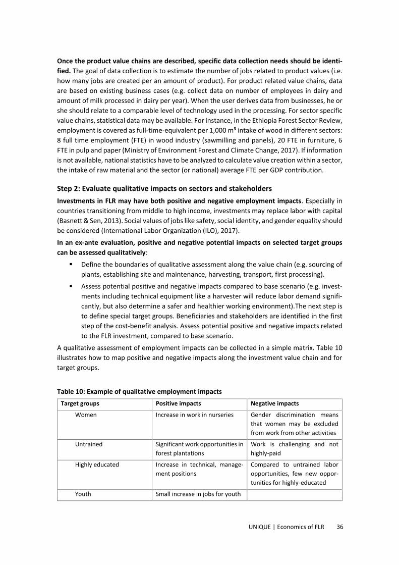
UNIQUE | Economics of FLR 36
Once the product value chains are described, specific data collection needs should be identi-fied. The goal of data collection is to estimate the number of jobs related to product values (i.e.how many jobs are created per an amount of product). For product related value chains, dataare based on existing business cases (e.g. collect data on number of employees in dairy andamount of milk processed in dairy per year). When the user derives data from businesses, he orshe should relate to a comparable level of technology used in the processing. For sector specificvalue chains, statistical data may be available. For instance, in the Ethiopia Forest Sector Review,employment is covered as full-time-equivalent per 1,000 m³ intake of wood in different sectors:8 full time employment (FTE) in wood industry (sawmilling and panels), 20 FTE in furniture, 6FTE in pulp and paper (Ministry of Environment Forest and Climate Change, 2017). If informationis not available, national statistics have to be analyzed to calculate value creation within a sector,the intake of raw material and the sector (or national) average FTE per GDP contribution.
Step 2: Evaluate qualitative impacts on sectors and stakeholdersInvestments in FLR may have both positive and negative employment impacts. Especially incountries transitioning from middle to high income, investments may replace labor with capital(Basnett & Sen, 2013). Social values of jobs like safety, social identity, and gender equality shouldbe considered (International Labor Organization (ILO), 2017).In an ex-ante evaluation, positive and negative potential impacts on selected target groupscan be assessed qualitatively: Define the boundaries of qualitative assessment along the value chain (e.g. sourcing of
plants, establishing site and maintenance, harvesting, transport, first processing). Assess potential positive and negative impacts compared to base scenario (e.g. invest-
ments including technical equipment like a harvester will reduce labor demand signifi-cantly, but also determine a safer and healthier working environment).The next step isto define special target groups. Beneficiaries and stakeholders are identified in the firststep of the cost-benefit analysis. Assess potential positive and negative impacts relatedto the FLR investment, compared to base scenario.
A qualitative assessment of employment impacts can be collected in a simple matrix. Table 10illustrates how to map positive and negative impacts along the investment value chain and fortarget groups.
Table 10: Example of qualitative employment impactsTarget groups Positive impacts Negative impacts
Women Increase in work in nurseries Gender discrimination meansthat women may be excludedfrom work from other activities
Untrained Significant work opportunities inforest plantations
Work is challenging and nothighly-paid
Highly educated Increase in technical, manage-ment positions
Compared to untrained laboropportunities, few new oppor-tunities for highly-educated
Youth Small increase in jobs for youth

UNIQUE | Economics of FLR 37
GDP and tax contributionsThe macroeconomic implications of an FLR investment can also be included, particularly theirimpact on GDP and tax revenues. It is important to note that neither GDP nor tax revenuesshould be included in the net value calculation of a project that are used to estimate the pro-ject’s total economic value. Taxes represent flow of resources from one party to another andare thus a net zero in terms of total economic value created.GDP is the total economic output of a given jurisdiction, most often calculated at the countrylevel. The contribution of a specific investment to a country’s GDP can be estimated; this is onlya helpful calculation to make in the case of large investments. In addition to the GDP contribu-tion of the investment itself, an investment is likely to have significant indirect contributions toGDP, for instance through increasing consumer spending or encouraging growth in downstreamsectors. In order to estimate indirect impact on GDP, a multiplier can be used; e.g. for every US$1 of investment, GDP increases by US$ 5. The multiplier is equal to: 1 / (1 – the marginal pro-pensity to consume). The marginal propensity to consume should be drawn from country eco-nomic data. If more accuracy is needed, a marginal propensity to consume can be estimated ona regional or other jurisdictional basis.Most investments will also increase a jurisdiction’s tax revenues. To estimate change in reve-nues, a thorough analysis of the relevant tax policies (at national, state, and local levels) mustbe completed in order to understand all relevant taxes. All tax policies, including capital gainstax, income tax, foreign investment tax, payroll tax, and sales tax, should be accounted for.
Opportunity costsOpportunity costs represent the costs and benefits of activities that would have taken place ifthe FLR investment did not take place. For example, if a degraded pasture land was not refor-ested, it would have continued to provide grazing area to cattle and therefore income to thecattle owner. Opportunity costs are important to include as it allows the user to compare differ-ent investments and understand the full costs and benefits of an investment.Under this framework, opportunity cost is accounted for by developing a business as usualscenario. The business as usual scenario should estimate all of the costs and benefits that wouldaccrue without the proposed investment, as well as can be predicted. If an FLR investment re-stricts economic activities in a particular area, then the business as usual scenario should includethe forgone revenues or other benefits that actors would have received.
BiodiversityBiodiversity is defined by the Convention on Biological Diversity as “the variability among liv-ing organisms from all sources including, terrestrial, marine and other aquatic ecosystems andthe ecological complexes of which they are part; this includes diversity within species, be-tween species and of ecosystems” (CBD 1992). Biodiversity is the underpinning for ecosystemservices. Attempts have been made to translate global biodiversity and associated ecosystemservices into economic values, e.g. (Costanza et al., 1998). Attempts at monetization typicallyresult in values that underestimate the importance of biodiversity or result in values that are

UNIQUE | Economics of FLR 38
not convincing to decision-makers. However, that does not mean that the importance of biodi-versity should be removed from decision-making processes. Instead of valuing biodiversity ineconomic terms, the authors propose that impacts on biodiversity be considered through a riskand opportunity approach. In specific cases where certain biodiversity values are easily linkedto specific ecosystem services (e.g. tourism values) there may be scope for some valuation.
Figure 11 provides an overview of the approach proposed to assess biodiversity values in thelandscape, identify opportunities, and mitigate threats to biodiversity. A full methodology forassessing biodiversity values can be found in Annex 3.
Figure 11: Step-wise approach for biodiversity assessment
Tier 3 analysis: Incorporating spatially-explicit dataTier 1 and Tier 2 analysis rely on one-hectare models that do not vary according to specificconditions within that hectare. For many purposes, this level of detail is sufficient to providethe user with an adequate level of confidence about the results. However, in other cases, it maybe necessary to increase the accuracy of the results by adjusting the one-hectare models de-pending on local conditions. Within a large project area, conditions can vary substantially, withsignificant effect on the ecosystem function.In order to incorporate precise local conditions and modify the outputs of the one-hectaremodel, users should divide or stratify the project areas into smaller units with shared charac-teristics. Stratification is a tool for minimizing sampling errors and increasing precision. The prin-ciple behind stratification is to group project implementation areas into relatively homogenousunits. This reduces the sample size required to meet defined precision levels. There is no rulefor ideal number of strata to have in project, but it is recommended to have minimum possible(4 to 6) with more effective criteria. Strata should be developed based on criteria that will havethe greatest impact on the costs or benefits in the project area.The most important physical attributes in FLR projects typically are: land cover type, elevationzone, slope, agro ecological zone, annual average precipitation, temperature, and soil type.Additionally, variables like current land use, presence of particular groups of people, and dis-tance from human settlements or roads can be also used as criteria for stratification.
1. Identify prioritybiodiversity values
and threats onlandscape level
2. Assess impactson biodiversityacross different
scenarios
3. Decide whetherto monetize
certain values

UNIQUE | Economics of FLR 39
Drawing the boundaries of every strata is most effective using a GIS program. In case projectspecific data are not available, the following variables can be downloaded freely and used forthe stratification:14
Aspect and position of hill slopes - Sites differing in aspect and position on a hill slopeare also stratified as tree growth varies in relation to these factors. For example, a standon the south side may have greater productivity than one on the north aspect.
Altitude - Forest blocks are selected within altitudinal ranges above mean sea level asvegetation types differ according to altitudinal variation. It is sensible to design elevationstrata that represent forests within certain range in altitude.
Physical and administrative boundaries – it is useful to consider if policy are different inthis admin units that affect the survival or growth of trees.
Soil texture / composition – Soil plays important role in agriculture, forest or any landbased project. Thus, it is important to categorize it on their effect on growth.
Precipitation – Average annual Precipitation classes categories that are relevant togrowth of trees or crop productivity.
The user should then determine how characteristics of the separate strata affect outputs ofthe economic models, and incorporate these effects.
3.3 Step 3: Data collectionIf input data come from reliable, local, and up-to-date sources, the level of confidence in thecost-benefit analysis will increase. On the otherhand, data collection can be expensive and time-consuming. The costs of data collection should beweighed against the need for accuracy, depend-ing on the purpose of the analysis.
Identify data needs and sourcesThe user must first identify all data needs basedupon calculations to be made under Step 2.Methodologies for estimating prices and quanti-ties should be elaborated at this stage in order to ensure that all needed data are collected.Necessary inputs for each calculation are determined. Potential sources and means of collectionfor every data input should be identified. This step should distinguish between primary data thatwill be collected “from the field” and areas where benchmark data will be used.
14 Physical and administrative boundaries can be found at: https://gadm.org/data.html; soil texture and compositioncan be found at : http://www.fao.org/soils-portal/soil-survey/soil-maps-and-databases/harmonized-world-soil-data-base-v12/en/; precipitation can be found at : http://www.worldclim.org/; and altitude and aspect can be found athttp://www.diva-gis.org/Data or https://asterweb.jpl.nasa.gov/gdem.asp

UNIQUE | Economics of FLR 40
Collect field dataHaving determined data needs and sources, the user should collect primary data. Differencesbetween predicted and actual data sources should be carefully documented. The data collectorshould also document any potential sources of uncertainty and estimate an “error range,” orthe percentage by which the collected data could be incorrect. Upon finishing data collection,remaining data gaps must be carefully noted.
Benchmark dataIn terms of costs and expected revenues, it is difficult to generalize across countries and FLRactivity types, as there is wide variance.
Table 11 provides an overview of expected financial costs and revenues for FLR activity types ona per hectare basis. Project-specific circumstances (e.g. country, exact project activities) varyfrom case to case, meaning that some FLR projects may fall outside of the ranges provided. Theestimates offer users a sense of the scale of potential costs and revenues and the timing andfrequency of revenues. Aside from provisioning services, this table does not include ecosystemservice values.
Table 11: Generalized costs and benefits for FLR activity types per hectare (US$)
Initial invest-ment
Annualmainte-nance
Harvestcost
Totalrevenues
Timing of reve-nues
IRR
Planted for-ests and
woodlands
1,000 –2,000 200 – 500
2,000–
4,000
8,000–
15,000
Thinnings fromyear 3; final
harvest yr 7-20
5-15%
Natural re-generation /ANR / activeregeneration
0 – 2,000 0 – 100 N/A N/A N/A N/A
Sustainableforest man-
agement50 – 200 50 – 100 200 –
1,000500 –3,000 Annual 15-
50+%
Agroforestry 1,000 –5,000
200 –1,500
500 –1,500
5,000–
20,000
Variable; manytree-based
crops from yr 3
10-25%
Soil restora-tion* 10 – 100 5 – 100 0 200 –
3,000Annual or
more frequent10-
50+%Source: Authors‘ calculations; soil restoration amounts are additional to existing agricultural activities
Planting forests and establishing woodlands requires significant upfront investments, primar-ily for seedlings, labor, infrastructure, and planting equipment. Annual maintenance – pruning,weeding, pest management, fire prevention – is crucial to ensure future returns. Depending onthe tree species rotation length of the plantation, thinnings may happen one to three times,usually starting during year three or four; this generates some revenues in early years. However,

UNIQUE | Economics of FLR 41
the majority of the revenues occur at final harvest, anywhere between years seven and twenty(or even longer, depending on the tree species). The combination of upfront investment andback loaded revenues creates liquidity gaps and financing challenges for such investments.Natural regeneration, assisted natural regeneration, and active regeneration vary in the in-tensity of planting and management of the planted species. The primary financial cost of nat-ural regeneration is simply in fencing off the protected area. However, there may be a significantopportunity cost from natural regeneration from foregone economic activities. ANR and activeregeneration imply a higher number of planted individuals per hectare, and thus higher costs.SFM can be a highly profitable activity, with relatively low upfront investment costs – typicallyfor equipment and labor. Depending on the forest management regime, revenues can beginimmediately.Agroforestry has the highest variability as the chosen crop combinations imply significantlydifferent investment volumes. Expenses include seedlings, labor, equipment, and infrastruc-ture. A silvopastoral system, for example, has relatively low upfront investment. Establishmentof a cocoa system, on the other hand has much higher costs. Maintenance costs are also high,typically for fertilizer (if relevant) and labor. With annual crops, revenues may start from yearone, in systems involving tree crops (e.g. coffee or cocoa) harvest may begin later. The highinvestment associated with agroforestry can result in high returns.Soil restoration activities also vary significantly (e.g. use of organic fertilizer, no-till farming),but tend to have relatively low costs: labor, inputs, and equipment. Most activities result inrevenues during the first year at the time of harvest; depending on the country and commodity,harvest may occur more than one time per year.
Refine methodologies, recollect dataIt may be the case that a user is unable to collect all necessary data from either primary orbenchmark data sources. In this case, the user should return to Step 2 in order to refine meth-odologies. Data need identification and collection should then be restarted.
3.4 Step 4: Analysis of costs and benefitsHaving determined costs and benefits over time, the user should construct a model, estimat-ing the flow of economic and/or financial value over time. In simple terms, this will look similarto Table 12. Models can be constructed for the project as a whole – the total economic value ofthe project – and for individuals or groups of stakeholders. It may be desirable to understandthe costs and benefits for a specific stakeholder, for example, a private investor.
Table 12: Simplified net values model (US$)Year 0 1 2 3 4 5 6 7
Costs (1,000) (300) (300) (300) (300) (300) (300) (300)
Benefits 100 300 300 600 600 600 600 600
Total (900) 0 0 300 300 300 300 300

UNIQUE | Economics of FLR 42
Determining the timing of costs and benefits is central to the analysis in order to account forthe time value of money. The idea that costs and benefits have different values depending ontime is a central concept in economics. With a few rare exceptions, benefits received today havemore value than benefits received in the future. Future values are discounted using a discountrate so that values at different times can be easily compared. This is done by assigning a weightto future events based on society’s preference for events that occur at different points in time.This allows a decision-maker to determine tradeoffs between different investments under con-sideration. Determining the discount rate is a difficult and potentially controversial element ofa cost-benefit analysis because it has a large impact on the perceived value of a project.A discount rate can be calculated through a few different methodologies, depending on theuser. A private company or investor typically uses its weighted average cost of capital (WACC)as its discount rate. WACC represents the cost that a company pays to finance an investment,including both equity and debt contributions to the investment.Public actors will use a different means of determining the appropriate discount rate. The moststraightforward way to choose the discount rate is to set it to the nominal rate of governmentreturn on bonds minus expectations of inflation.However, in many cases, a public sector entity will calculate a discount rate through othermeans in order to incorporate the preferences of its members. National governments usevastly different discount rates, ranging from 3 to 15%, while other bodies use even lower rates,or apply a lower rate for values far in the future (Harrison, 2010). Choosing a discount rate thatincludes subjective preferences is as much of an art as a science, and there is significant debateabout the methodology to choose an appropriate rate. The rate depends on the preferences ofrelevant stakeholders. A young community may, for example, prefer future benefits over currentbenefits. An older community may prefer the opposite. Smallholders, especially if they are notwealthy, will likely have immediate cash needs and therefore a high discount rate. If the userwants to take inter-generational preferences into account – the relative value of the preferencesof people who have not been born yet – then a discount rate of close to zero or one that declineswith time is necessary (Cropper, 2013).In the context of FLR investments, it is important to note that environmental benefits typicallyaccrue relatively far in the future. Using a high discount rate will decrease the relative monetaryvalue of environmental benefits in FLR investments. However, the desire to include the mone-tary of value environmental benefits should be weighed against the immediate needs of a coun-try or community. It may be appropriate to test how different discount rates affect the project’svalue via a sensitivity analysis (cf. Section 3.4.2).
Relevance of different indicatorsOnce a model is constructed, the user can conduct a variety of calculations for different typesof analysis. Definitions and equations for these indicators can be found in Annex 1. The rele-vance of different indicators is described below.Net present value (NPV) describes the value of an investment discounted to present terms.Any positive NPV value means that the discounted benefits from the project are greater than

UNIQUE | Economics of FLR 43
the discounted costs – i.e. it is a worthwhile investment. NPVs of similar investments can becompared to determine which is more profitable. The downside of using NPV is that it is difficultto compare the profitability of investments of different sizes. For instance, the NPV of a US$ 1million investment may be greater than the NPV of a US$ 1 investment, but the effectiveness ofeach dollar invested is not apparent from NPV.The internal rate of return (IRR), on the other hand, describes the effectiveness of each dollarspent and allows the user to compare profitability of investments of different sizes. Any IRRwith a positive value means that the discounted benefits of the project are greater than thediscounted costs. What a public or private investor determines to be an acceptable IRR dependson their other investment options and their perception of risk.Benefit/cost ratio is another effective indicator for analyzing the effectiveness of invested re-sources. A benefit/cost ratio that is greater than one implies that total benefits are greater thantotal costs.Return on investment (ROI) and return on equity (ROE) are indicators that also measure theefficiency of resources invested. ROI tells the user the profitability return for every dollar in-vested. ROE is similar to ROI, with one important difference, except that it measures only thereturn on equity invested.The initial investment amount is the amount of financial resources that are needed in the firststage of the investment. For smallholders and other actors in the forestry and agricultural sec-tors, borrowing money or otherwise attracting investors can be a key challenge. Therefore, thisis often a key indicator.Breakeven point is the time at which the cumulative cash flows of the project shift from neg-ative to positive. In addition to indicating the payback period, this is a helpful indicator as it islinked to the amount of time needed to repay an external investment.
Dealing with uncertaintyCost benefit analyses inevitably involve a degreeof uncertainty as they are an attempt to estimateor model the future. There are a few strategies toaccount for uncertainty. Any cost-benefit analysisshould be clear about key assumptions that itmakes in order to make its calculations. An exter-nal party reading the analysis should be able toeasily identify input variables and on what basisthe author of the report chose the value.A cost-benefit analysis should account for uncer-tainty by conducting a sensitivity analysis. Sensitivity analyses test how the calculations of themodel change if key input data changes. This allows the user to understand under which condi-tions their investment is feasible or not and the variables that have the greatest impact on aproject’s success. A handful of input variables that have a large impact on the costs and benefitsof the investment should be chosen. For each selected variable, reasonable alternatives should
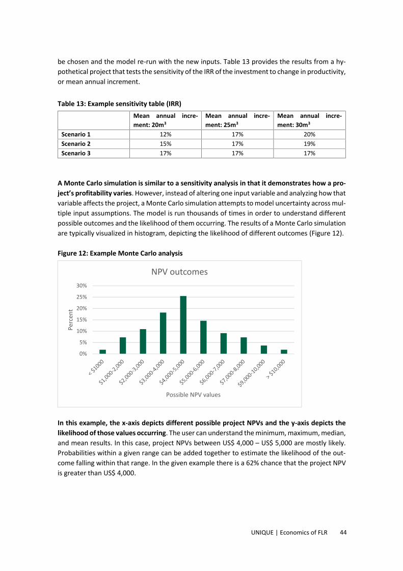
UNIQUE | Economics of FLR 44
be chosen and the model re-run with the new inputs. Table 13 provides the results from a hy-pothetical project that tests the sensitivity of the IRR of the investment to change in productivity,or mean annual increment.
Table 13: Example sensitivity table (IRR)Mean annual incre-ment: 20m3
Mean annual incre-ment: 25m3
Mean annual incre-ment: 30m3
Scenario 1 12% 17% 20%Scenario 2 15% 17% 19%Scenario 3 17% 17% 17%
A Monte Carlo simulation is similar to a sensitivity analysis in that it demonstrates how a pro-ject’s profitability varies. However, instead of altering one input variable and analyzing how thatvariable affects the project, a Monte Carlo simulation attempts to model uncertainty across mul-tiple input assumptions. The model is run thousands of times in order to understand differentpossible outcomes and the likelihood of them occurring. The results of a Monte Carlo simulationare typically visualized in histogram, depicting the likelihood of different outcomes (Figure 12).
Figure 12: Example Monte Carlo analysis
In this example, the x-axis depicts different possible project NPVs and the y-axis depicts thelikelihood of those values occurring. The user can understand the minimum, maximum, median,and mean results. In this case, project NPVs between US$ 4,000 – US$ 5,000 are mostly likely.Probabilities within a given range can be added together to estimate the likelihood of the out-come falling within that range. In the given example there is a 62% chance that the project NPVis greater than US$ 4,000.
0%
5%
10%
15%
20%
25%
30%
Perc
ent
Possible NPV values
NPV outcomes

UNIQUE | Economics of FLR 45
4 CONCLUSIONS
Economically sound business models for sustainable land use activities can provide strong ar-guments for both, investors and policy makers. These arguments will help advancing from dis-cussions to implementation. The outputs of a cost-benefit analysis seem clear: one scenario willbe more profitable than others. However, taking a decision is not as simple as selecting the sce-nario with the greatest total net benefits. Cost-benefit analyses are only one tool amongst manyin decision-making.A cost benefit analysis can help designing specific investments, programs and supporting pol-icies. For example, financial incentives for different stakeholder groups can be based on a costbenefit analysis: it will elucidate how different stakeholders bear the costs and benefits of aninvestment. It may also reveal, for instance, that landowners implementing a watershed protec-tion scheme have higher costs than benefits to the landowners. In this case, the analysis canhelp identifying potential financial incentives for these landowners. If quality input data wereavailable, the analysis should provide a comprehensive understanding of the tradeoffs underdifferent scenarios. To inform decision-making key inputs and outputs should be presented inan easy to understand manner.The user should be prepared that the results of a cost benefit analysis can be controversialand may be met with disbelief and questioning the validity of the results. For this reason, onehast to be aware of the limitations. Once the analysis has been completed, it should be validatedthrough consultations with different stakeholders. In addition to confirming the accuracy or im-proving accuracy, validation is an important step to encourage stakeholder buy-in. The analysiswill also make clear the scale of investment needed, so considering possible sources of invest-ment is another important next step.
Limitations of cost-benefit analyses as a decision-making toolFirst, the analysis is based on a number of assumptions that have a varying degree of confi-dence. Ideally, key stakeholders are consulted during the data collection process to improve theaccuracy and increase their buy-in. Climate change and other unforeseen events may affectproductivity in difficult to predict ways, which should be noted. Stated assumptions should gobeyond cost, price, and productivity assumptions to include social and/or political assumptions.Second, monetizing environmental and social benefits is a difficult and, at times, controversialtopic. Stakeholders may value environmental benefits differently and therefore dispute the find-ings of the analysis. For example, some prioritize global ecosystem services like GHG mitigationwhile another prioritizes local benefits as reducing soil erosion. Selecting a discount rate – andthus prioritizing near-term versus long-term benefits – is an inherently subjective decision.Lastly, the value of some environmental benefits, such as supporting biodiversity, are often in-tentionally excluded because they cannot be monetized. However, although biodiversity maynot be valued in a cost benefit analysis, it can still be included in decision-making.Third, there may be political or social considerations that are difficult to monetize and includein the analysis. As much as stakeholders would expect that policy makers select the option thatproduces the greatest benefits for all, this does not occur in the real world. Benefits to one groupmay be valued more than benefits to another group because of political reasons, although thisis not included in the cost benefit analysis.

UNIQUE | Economics of FLR 46
Last, a common misperception of cost benefit analysis is that it is the important decision-mak-ing tool for private investors. While the expected profitability of an investment is of course im-portant for investors, it is one of many criteria. Investors are not just investing into an Excelmodel; they are investing in people and companies, who are operating in complex and some-times risky environments. The creditworthiness of an investee – their credit history, the collat-eral they can provide, the size of their business, their experience – is typically more importantthan the expected IRR of a business model. Macroeconomic conditions, especially political riskand foreign currency volatility, will also be investigated by investors.The level of detail of analysis should inform immediate next steps. If a Tier 1 analysis was com-pleted, relying primarily on benchmark data, the user may not be very confident of the finalresults. If such a high level analysis suggests that investment scenarios could be profitable, thena Tier 2 or Tier 3 analysis should be completed in order to ensure confidence in the results.
OutlookSuccessful implementation of FLR activities at a landscape level has significant potential fordifferent kinds of economic benefits, which accrue to different stakeholders. A full economicanalysis tries to capture not only monetary, but also non-monetary values from different eco-system services. Simply adding up these figures would result mislead, but ignoring such impactsand values would create an incomplete picture of the benefits. The compromise should be adifferentiated assessment, based on the purpose of the assessment and the needs of those re-questing it. Independent of beneficiary, purpose and level of detail, any assessment of costs andbenefits should be robust and guided by the principles of conservativeness and credibility.
Robust and credible estimations of the economic impacts and the costs of inaction can bepowerful instruments to stimulate the implementation of FLR on the ground. In many cases,policy makers still need to be convinced of the various benefits of such investments and theirdimension. It can help translate country pledges into action on the ground and weigh alternativescenarios, e.g. in the context of bi- and multilateral development cooperation programs. It canalso refine the results of FLR opportunity assessments, structure and inform discussions amongstakeholders and help identifying trade-offs between different options (including inaction).Public and private investors considering FLR need quick, but reliable information on the finan-cial dimension and other impacts. Financial analyses are straightforward and provide basic in-formation such as investment needs, returns on investment, internal rates of return, and cashflow profiles. However, particularly impact investors are increasingly interested in also havingestimations of the expected environmental and social impacts of their activities.
Economic analyses can help identifying trade-offs between different FLR options for identifiedlandscapes. At landscape level there will be different options for starting restoration processes,with significant impacts on investment needs and impacts. In light of uncertainties, assumptionsand different benefits accruing at different points of time, its results are not sufficient to deter-mine the most appropriate FLR strategy for a given landscape. Ideally, the proposed methodol-ogy builds on and complements an opportunity assessment with a stakeholder process.

UNIQUE | Economics of FLR 47
5 LITERATURE AND SOURCESAronson, J., Clewell, A. F., Blignaut, J. N., & Milton, S. J. (2006). Ecological restoration: A new
frontier for nature conservation and economics. Journal for Nature Conservation, 14(3–4), 135–139. https://doi.org/10.1016/j.jnc.2006.05.005
Balmford, A., Rodrigues, A. S. L., Walpole, M., ten Brink, P., Kettunen, M., Braat, L., & de Groot,R. (2008). The Economics of Ecosystems and Biodiversity: Scoping the Science. Cambridge,UK: European Commission, 39(1), 186–188. https://doi.org/10.1093/erae/jbr052.
Basnett, Y., & Sen, R. (2013). What do empirical studies say about economic growth and jobcreation in developing countries? (September), 38. https://assets.publishing.ser-vice.gov.uk/media/57a08a2340f0b652dd0005a6/Growth_and_labour_absorption.pdf
Beeli, P., Anderson, J., Barnum, H., Dixon, J., & Tan, J.-P. (2001). Economic Analysis of InvestmentOperations: Analytical Tools and Practical Applications. World Bank. http://docu-ments.worldbank.org/curated/en/792771468323717830/pdf/298210REPLACEMENT.pdf
Bockel, Louis; Grewer, Uwe; Fernandez, C. (2013). EX-ACT User Manual: Estimating and Target-ing Greenhouse Gas Mitigation in Agriculture. Retrieved from http://www.fao.org/filead-min/templates/ex_act/pdf/Technical_guidelines/EX-ACTUserManuaFi-nal_WB_FAO_IRD.pdf
Bonn Challenge. (2018). Getting Started with the Bonn Challenge, 1(866), 3–4.https://www.unece.org/fileadmin/DAM/timber/meetings/2018/20180621/Get-ting_Started_with_the_Bonn_Challenge_2018.pdf
Ciccarese, L., Mattsson, A., & Pettenella, D. (2012). Ecosystem services from forest restoration:Thinking ahead. New Forests, 43(5–6), 543–560. https://doi.org/10.1007/s11056-012-9350-8
Costanza, R., d’Arge, R., de Groot, R., Farber, S., Grasso, M., Hannon, B., […] van den Belt, M.(1998). The value of the world’s ecosystem services and natural capital. Ecological Eco-nomics, 25(1), 3–15. https://doi.org/10.1016/S0921-8009(98)00020-2
Cropper, M. L. (2013). How Should Benefits and Costs Be Discounted in an Intergenerational Con-text? SSRN. https://doi.org/10.2139/ssrn.2199511
Defra. (2007). An introductory guide to valuing ecosystem services. Forestry, 68.https://doi.org/10.1111/j.1468-0327.2007.00195.x
Desmet, P. & Govers, G. (1996). A GIs procedure for automatically calculating the USLE LS factoron topographically complex landscape units. Journal of Soil and Water Conservation,51(5), 427–433. https://www.researchgate.net/publication/233425999_A_GIS_proce-dure_for_automatically_calculating_the_USLE_LS_factor_on_topographically_com-plex_landscape_units
FAO, & UNCCD. (2015). Sustainable financing for forest and landscape restoration. Retrievedfrom papers3://publication/uuid/712EA118-2FC1-4F3D-8D17-A97F84E21500
Gibbs, H. K., & Salmon, J. M. (2015). Mapping the world’s degraded lands. Applied Geography,57, 12–21. https://doi.org/10.1016/j.apgeog.2014.11.024

UNIQUE | Economics of FLR 48
Hamrick, K., & Gallant, M. (2017). Unlocking Potential State of the Voluntary Carbon Markets2017 Supporter Sponsors Initiative for Sustainable Forest Landscapes, 52. Retrieved fromhttp://www.forest-trends.org/dir/em_newsletter
Hanson, Craig; Buckingham, Kathleen; Dewitt, Sean; and Laestadius, L. (2015). The RestorationDiagnostic. World Resources Institute, 1–10. https://doi.org/978-1-56973-875-7
Harrison, M. (2010). Valuing the Future: The social discount rate in cost-benefit analysis. Austral-ian Government: Productivity Commission. https://www.pc.gov.au/research/support-ing/cost-benefit-discount
International Labor Organization (ILO). (2017). World Employment Social Outlook.https://www.ilo.org/wcmsp5/groups/public/---dgreports/---dcomm/---publ/docu-ments/publication/wcms_541211.pdf
IPCC. (2007a). Climate Change 2007: Impacts, Adaptation and Vulnerability.https://www.ipcc.ch/pdf/assessment-report/ar4/wg2/ar4-wg2-intro.pdf
IPCC. (2007b). Climate Change 2007. Change, 20 November, 12-17.https://doi.org/http://dx.doi.org/10.1017/CBO9780511546013
IUCN. (n.d.). What is FLR. Retrieved September 12, 2018, from https://infoflr.org/what-flrKluve, J., & Stoterau, J. (2014). A Systematic Framework for Measuring Employment Impacts.
GIZ. https://energypedia.info/images/5/54/A_Systematic_Framework_for_Measu-ring_Employment_Impacts_of_Development_Cooperation_Interventions.pdf
MEA, M. E. A. (2005). Ecosystems and Human Well-Being Ecosystems and Human Well-Being.https://doi.org/10.1196/annals.1439.003
Ministry of Environment Forest and Climate Change. (2017). Ethiopia Forest Sector Review: Fo-cus on commercial forestry and industrialization.https://www.google.com/url?sa=t&rct=j&q=&esrc=s&source=web&cd=2&ved=2ahUKEwjg8Zu_gc_eAh-VMKcAKHfL2ACIQFjABegQIBxAC&url=https%3A%2F%2Fmefcc.gov.et%2Fwp-con-tent%2Fplugins%2Fdownload-attachments%2Fincludes%2Fdown-load.php%3Fid%3D2090&usg=AOvVaw0OpglThEm8HJI7Y3URLvfy
Pan, Y., Birdsey, R. A., Fang, J., Houghton, R., Kauppi, P. E., Kurz, W. A., … Hayes, D. (2011). Alarge and persistent carbon sink in the world’s forests. Science, 333(6045), 988–993.https://doi.org/10.1126/science.1201609
Pascal, U., & Muradian, R. (2010). TEEB Chapter 5 The Economics of Valuing Ecosystem Servicesand Biodiversity. …of Ecosystems and …, (March). Retrieved from http://ca-dair.aber.ac.uk/dspace/handle/2160/12537
Pereira, H. M., Leadley, P. W., Proença, V., Alkemade, R., Scharlemann, J. P. W., Fernandez-Man-jarrés, J. F., … Hutyra, L. R. (2010). Scenarios for global biodiversity in the 21st century.Science, 330(6010), 1496–1501. https://doi.org/10.1126/science.1196624
Pistorius, T., & Kiff, L. (2017). From a biodiversity perspective: risks, trade- offs, and internationalguidance for Forest Landscape Restoration From a biodiversity perspective : risks, trade-offs, and international guidance for Forest Landscape Restoration, (January).https://www.unique-landuse.de/images/publications/vereinheit-licht/UNIQUE_FLR_from_a_biodiversity_perspective_2017.pdf

UNIQUE | Economics of FLR 49
Rodrigues, R. R., Lima, R. A. F., Gandolfi, S., & Nave, A. G. (2009). On the restoration of highdiversity forests: 30 years of experience in the Brazilian Atlantic Forest. Biological Conser-vation, 142(6), 1242–1251. https://doi.org/10.1016/j.biocon.2008.12.008
Rwanda, M. of N. R.-. (2016). Forest Landscape Restoration Opportunity Assessment for Rwanda.(W. MINIRENA (Rwanda), IUCN, Ed.).http://cmsdata.iucn.org/downloads/roar_web_version.pdf
Rypdal, K., Paciornik, N., Eggleston, S., Goodwin, J., Irving, W., Penman, J., & Woodfield, M.(2006). Chapter 1: Introduction to the 2006 Guidelines. 2006 IPCC Guidelines for NationalGreenhouse Gas Inventories, 12. Retrieved from http://www.ipcc-nggip.iges.or.jp/pub-lic/2006gl/pdf/1_Volume1/V1_1_Ch1_Introduction.pdf
Stocking, M. A. (2001). Land Degradation. International Encyclopedia of the Social & BehavioralSciences, 8242–8247. https://doi.org/10.1016/B0-08-043076-7/04184-X
TEEB. (2010). Mainstreaming the economics of nature. Environment. Retrieved fromhttp://www.iges.or.jp/jp/news/topic/pdf/1103teeb/teeb_synthesis_j.pdf
UNDP. (2016). Pursuing the 1.5 °C Limit Benefits & Opportunities. http://www.undp.org/con-tent/dam/undp/library/Climate%20and%20Disaster%20Resilience/Cli-mate%20Change/Pursuing_1-5C-Limit.pdf
Verdone, M. (2015). A Cost-Benefit Framework for Analyzing FLR Decisions. Retrieved fromhttps://portals.iucn.org/library/sites/library/files/documents/2015-018.pdf
Vergara, W., Lomeli, L. G., Rios, A. R., Isbell, P., Prager, S., & De Camino, R. (2017). The EconomicCase for Landscape Restoration in Latin America. https://www.wri.org/publication/eco-nomic-case-for-restoration-20x20
Watson, R., Noble, I., Bolin, B., Ravindranath, N. H., Verardo, D., & Dokken, D. (2000). Land Use,Land-Use Change and Forestry. Cambridge: IPCC. http://www.ipcc.ch/ipccre-ports/sres/land_use/index.php?idp=0
Wischmeier, W. H., Smith, D. D. (1981). Predicting rainfall erosion losses. Supersedes AgricultureHandbook 282, 282(537), 1–69. https://doi.org/10.1029/TR039i002p00285
World Bank. (2017). Shadow price of carbon in economic analysis Guidance note, 1–9.World Bank. (2017). Shadow price of carbon in economic analysis Guidance note, 1–9.World Bank. (2017). Shadow price of carbon in economic analysis Guidance note, 1–9.World Bank. (2017). Shadow price of carbon in economic analysis. Guidance note, 1–9.
http://pubdocs.worldbank.org/en/911381516303509498/2017-Shadow-Price-of-Car-bon-Guidance-Note-FINAL-CLEARED.pdf
Wreford, A., Moran, D., & Adger, N. (2010). Climate change and agriculture: impacts, adaptationand mitigation. Source OECD Agriculture & Food, Volume 9. http://www.oecd.org/green-growth/climate-change-and-agriculture-9789264086876-en.htm
WRI (2011). A World of Opportunity A World of Opportunity for Forest and Landscape Restora-tion Forest and Landscape Restoration Opportunities. http://pdf.wri.org/world_of_op-portunity_brochure_2011-09.pdf
WRI; IUCN. (2014). A guide to the Restoration Opportunities Assessment Methodology (ROAM):Assessing forest landscape restoration opportunities at the national or sub-national level.Building, 1–43. https://cmsdata.iucn.org/downloads/roam_handbook_lowres_web.pdf

UNIQUE | Economics of FLR 50
ANNEX 1: GLOSSARY OF TERMSBenefit/cost ratioThis is an effective indicator for analyzing the effectiveness of invested resources. It is calculatedby dividing total discounted benefits by total discounted costs. A benefit/cost ratio that isgreater than one implies that total benefits are greater than total costs.
Bonn ChallengeA voluntary high-level policy approach which encourages countries to pledge degraded lands forthe global FLR movement. The Bonn Challenge was initiated by the German government as animplementation-focused approach complementary to the various formal negotiation processesunder the UN – in particular the UNFCCC, the UNDCCD and the CBD. It aimed at having by 2020more than 150 million hectares of the world's degraded and deforested lands in processes ofrestoration. Two associated regional initiatives have evolved out of the Bonn Challenge: theAFR100 initiative for Africa and the 20*20 initiative for Latin America.
Breakeven pointThe break-even point is the time at which the cumulative cash flows of the project shift fromnegative to positive.
Capital Expenditure (CAPEX)CAPEX items are durable goods that a company will use for more than one year. CAPEX includes,for example, the purchase of land, perennial seedlings, equipment, or infrastructure.
Carbon stock changeCarbon stock is the quantity of carbon contained in a “pool”, meaning a reservoir or systemwhich has the capacity to accumulate (“sink”) or release carbon (“source”). For forests, it refersto changes in its different pools, mainly in living biomass and soil, but also in dead wood andlitter (Watson et al., 2000).
Cost-benefit analysis (CBA)CBA is a decision-making tool that provides a systematic approach for quantifying and monetiz-ing the strengths (benefits) and weaknesses (costs) that helps decision makers decide betweenalternative investment options.
Discount rateThe interest rate used in discounted net value analysis to determine the present value of futurevalues. The higher the discount rate, the lower the present value of the future values.
Financial analysisA financial analysis takes the perspective of a single actor, often a private sector entity aimingat engaging into a FLR investment. It takes into account costs and benefits that are restricted tocash flows that can be directly monetized, such as upfront and management costs, increasedrevenues from products sold, and any fiscal incentives from the public sector. It helps in the

UNIQUE | Economics of FLR 51
process of deciding on investments and comparing the potential returns from the proposed FLRinvestment with alternative investment options.
Economic analysisEconomic analyses are carried out when a public sector entity is making an investment. They areused for calculating the diverse costs and benefits of a particular FLR activity. While financialanalyses compare benefits and costs to an enterprise, economic analyses compare the benefitsand costs to the whole economy, or to various actors.
Forest Landscape Restoration (FLR)FLR is defined as a long-term process of regaining ecological functionality and enhancing humanwell-being across deforested or degraded forest landscapes. It aims to restore a whole landscape‘forward’ to meet the present and future needs and to offer multiple benefits and land uses overtime (IUCN, n.d.). The Intergovernmental Science-Policy Platform on Biodiversity and EcosystemServices (IPBES) defined restoration as “any intentional activity that initiates or accelerates therecovery of an ecosystem from a degraded state.”
Forest / land degradationThe FAO defines degradation as “changes within the forest which negatively affect the structureor function of the stand onsite, and thereby lower the capacity to supply products and/or ser-vices.” (FAO 2006). Degradation can simply be described as any process which lowers the qualityof land, and as a consequence, impairs ecological functions and provision of ecosystem services.
Initial investment amountThe initial investment is the amount of financial resources that are needed in the first stage ofthe investment. Given that many large projects are financed in part from external sources, itdemonstrates the scale of resources that need to be raised from outside investors.
Internal rate of return (IRR)IRR is calculated using the NPV formula (see NPV definition below) and setting the NPV equal tozero, then solving for the discount rate. IRR describes the effectiveness of each dollar spent andallows the user to compare profitability of investments of different sizes. A positive value for IRRmeans that the discounted benefits of the project are greater than the discounted costs
Net present value (NPV)NPV describes the total value of the investment, discounted to present day terms. It is calculatedby modeling the net values into the future, discounted by the chosen discount rate:NPV = (Net values) / (1 + r)n
Where R is equal to the discount rate and N is equal to the period in years.
Operational expenditure (OPEX)OPEX refers to expenses for goods or services that are used during one year and are often re-lated to the management and maintenance of the investment. This could include, for example,hiring labor to prune a restored area or fire prevention activities.

UNIQUE | Economics of FLR 52
Return on investment (RoI)ROI tells the user the profitability return for every dollar invested. It is calculated using the fol-lowing formula:ROI = (benefits – costs) / total investment
Return on equity (RoE)ROE is another indicator that measures the efficiency of resources invested. ROE is similar toROI, with one important difference, as seen in the following formula:ROE = (benefits – costs) / total equity investedTherefore, ROE demonstrates the profitability return on equity invested into the project. Thistakes the perspective of a shareholder in the company and their expected return. The differencebetween ROI and ROE is determined by the amount of debt that is used to finance a project.
Total economic value (TEV)A measure to estimate and monetize all economic impacts of an investment. TEV recognizes thatbenefits and costs radiate far beyond the landowner or investor – from neighboring propertiesall the way to global impacts.
Weighted average cost of capital (WACC)WACC is one of the ways to calculate a discount rate, and is typically used by a private companyor investor. WACC represents the cost that a company pays to finance an investment, includingboth equity and debt contributions to the investment. WACC is calculated as follows:WACC = (E/V * Ke) + (D/V) * Kd * (1 – T)Where E = the market value of the firm’s equity; V= the market value of the firm’s equity anddebt; Ke = the cost of equity; D = the market value of the firm’s debt; Kd = the cost of debt; andT = the tax rate.
Working capitalWorking capital is related to short-term expenses for the purchase and sale of goods and is mostrelevant for companies that buy an unfinished product, add value, and then sell the product.
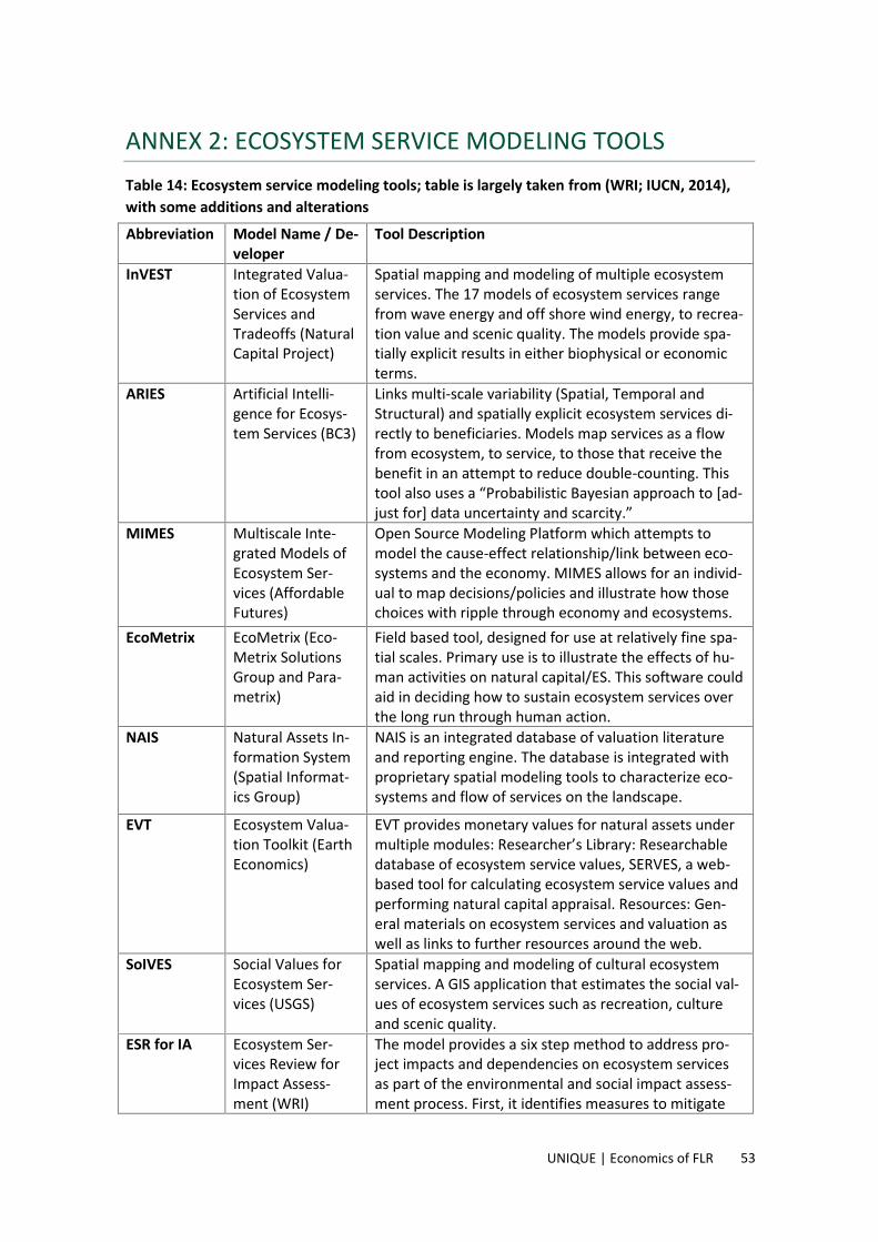
UNIQUE | Economics of FLR 53
ANNEX 2: ECOSYSTEM SERVICE MODELING TOOLSTable 14: Ecosystem service modeling tools; table is largely taken from (WRI; IUCN, 2014),with some additions and alterationsAbbreviation Model Name / De-
veloperTool Description
InVEST Integrated Valua-tion of EcosystemServices andTradeoffs (NaturalCapital Project)
Spatial mapping and modeling of multiple ecosystemservices. The 17 models of ecosystem services rangefrom wave energy and off shore wind energy, to recrea-tion value and scenic quality. The models provide spa-tially explicit results in either biophysical or economicterms.
ARIES Artificial Intelli-gence for Ecosys-tem Services (BC3)
Links multi-scale variability (Spatial, Temporal andStructural) and spatially explicit ecosystem services di-rectly to beneficiaries. Models map services as a flowfrom ecosystem, to service, to those that receive thebenefit in an attempt to reduce double-counting. Thistool also uses a “Probabilistic Bayesian approach to [ad-just for] data uncertainty and scarcity.”
MIMES Multiscale Inte-grated Models ofEcosystem Ser-vices (AffordableFutures)
Open Source Modeling Platform which attempts tomodel the cause-effect relationship/link between eco-systems and the economy. MIMES allows for an individ-ual to map decisions/policies and illustrate how thosechoices with ripple through economy and ecosystems.
EcoMetrix EcoMetrix (Eco-Metrix SolutionsGroup and Para-metrix)
Field based tool, designed for use at relatively fine spa-tial scales. Primary use is to illustrate the effects of hu-man activities on natural capital/ES. This software couldaid in deciding how to sustain ecosystem services overthe long run through human action.
NAIS Natural Assets In-formation System(Spatial Informat-ics Group)
NAIS is an integrated database of valuation literatureand reporting engine. The database is integrated withproprietary spatial modeling tools to characterize eco-systems and flow of services on the landscape.
EVT Ecosystem Valua-tion Toolkit (EarthEconomics)
EVT provides monetary values for natural assets undermultiple modules: Researcher’s Library: Researchabledatabase of ecosystem service values, SERVES, a web-based tool for calculating ecosystem service values andperforming natural capital appraisal. Resources: Gen-eral materials on ecosystem services and valuation aswell as links to further resources around the web.
SoIVES Social Values forEcosystem Ser-vices (USGS)
Spatial mapping and modeling of cultural ecosystemservices. A GIS application that estimates the social val-ues of ecosystem services such as recreation, cultureand scenic quality.
ESR for IA Ecosystem Ser-vices Review forImpact Assess-ment (WRI)
The model provides a six step method to address pro-ject impacts and dependencies on ecosystem servicesas part of the environmental and social impact assess-ment process. First, it identifies measures to mitigate

UNIQUE | Economics of FLR 54
Abbreviation Model Name / De-veloper
Tool Description
project impacts on the benefits provided by ecosys-tems. Second, it identifies measures to manage opera-tional dependencies on ecosystems.
MESP Marine EcosystemServices Partner-ship (Duke)
Database of publications that report economic outputsof ecosystem services. Provides an interactive map(through filters) to show publications by region. Thetool specifically targets oceanic and coastal (marine)ecosystem services and provides databases specified byregion/ecosystem.
Tessa Tessa (Bird Life In-ternational)
A site-specific look at ecosystem services. The tool al-lows for an “alternate state” which can be directly com-pared to with the current state of an ecosystem. Usesflow charts to map where the ecosystem services arebenefiting society.
Co$ting Na-ture
Co$ting Nature(King’s CollegeLondon and Ambi-oTEK)
Spatial mapping and modeling of multiple ecosystemservices using global coarse-resolution datasets. Under-stands ecosystem services as opportunity cost. This toolemphasizes the importance of conservation measures.
EnSym EnvironmentalSystems ModellingPlatform (State ofVictoria, Australia)
EnSym is an environmental systems modeling platformand framework for scientists and researchers to testand apply empirical and process-based scientific mod-els. EnSym provides users with an evidence-basedframework to support decision-makers on how andwhere to invest to maximize environmental outcomes.
LUCI Land Utilizationand Capability In-dicator (VictoriaUniversity of Wel-lington)
Formerly known as PolyScape. ”LUCI explores the capa-bility of a landscape to provide a variety of ecosystemservices. It compares the services provided by the cur-rent utilization of the landscape to estimates of its po-tential capability, and uses this information to identifyareas where change might be beneficial, and wheremaintenance of the status quo might be desirable”(quoted from website)
Wildlife Hab-itat BenefitsEstimationToolkit
WHBET (SpecificPaper) (Defendersof Wildlife & Colo-rado State Univer-sity)
Spreadsheet for monetary valuation (function transfer).Models include: residential property values and openspace, wildlife recreation, and total value of habi-tat/wetland services.
Envision Envision (OregonState University)
Open Source GIS-based tool for scenario based planningand environmental assessment. Able to complete “mul-tiagent modeling” to represent human decisions onlandscape simulations.
iTree ITree (US$A) Provides urban forest analysis and benefit assessmenttools. This tool specifically identifies ecosystem servicesfrom tree (be it a single tree or forested park, neighbor-hood, city or state). The tool aids in urban forest man-agement activities.
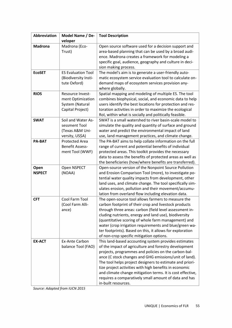
UNIQUE | Economics of FLR 55
Abbreviation Model Name / De-veloper
Tool Description
Madrona Madrona (Eco-Trust)
Open source software used for a decision support andarea-based planning that can be used by a broad audi-ence. Madrona creates a framework for modeling aspecific goal, audience, geography and culture in deci-sion making process.
EcoSET ES Evaluation Tool(Biodiversity Insti-tute Oxford)
The model's aim is to generate a user-friendly auto-matic ecosystem service evaluation tool to calculate on-demand maps of ecosystem services provision any-where globally.
RIOS Resource Invest-ment OptimizationSystem (NaturalCapital Project)
Spatial mapping and modeling of multiple ES. The toolcombines biophysical, social, and economic data to helpusers identify the best locations for protection and res-toration activities in order to maximize the ecologicalRoI, within what is socially and politically feasible.
SWAT Soil and Water As-sessment Tool(Texas A&M Uni-versity, US$A)
SWAT is a small watershed to river basin-scale model tosimulate the quality and quantity of surface and groundwater and predict the environmental impact of landuse, land management practices, and climate change.
PA-BAT Protected AreaBenefit Assess-ment Tool (WWF)
The PA-BAT aims to help collate information on the fullrange of current and potential benefits of individualprotected areas. This toolkit provides the necessarydata to assess the benefits of protected areas as well asthe beneficiaries (how/where benefits are transferred).
OpenNSPECT
Open NSPECT(NOAA)
Open-source version of the Nonpoint Source Pollutionand Erosion Comparison Tool (more), to investigate po-tential water quality impacts from development, otherland uses, and climate change. The tool specifically sim-ulates erosion, pollution and their movement/accumu-lation from overland flow including elevation data.
CFT Cool Farm Tool(Cool Farm Alli-ance)
The open-source tool allows farmers to measure thecarbon footprint of their crop and livestock productsthrough three areas: carbon (field level assessment in-cluding nutrients, energy and land use), biodiversity(quantitative scoring of whole farm management) andwater (crop irrigation requirements and blue/green wa-ter footprints). Based on this, it allows for explorationof non-crop specific mitigation options.
EX-ACT Ex-Ante Carbonbalance Tool (FAO)
This land-based accounting system provides estimatesof the impact of agriculture and forestry developmentprojects, programmes and policies on the carbon-bal-ance (C stock changes and GHG emissions/unit of land).The tool helps project designers to estimate and priori-tize project activities with high benefits in economicand climate change mitigation terms. It is cost effective,requires a comparatively small amount of data and hasin-built resources.
Source: Adapted from IUCN 2015
UNIQUE | Economics of FLR 56
ANNEX 3: APPROACH FOR ESTIMATING BIODIVERSITYVALUES
Identifying priority biodiversity value and threats on landscape levelTo assess biodiversity values, the target landscape should be screened in order to understandits biodiversity value. First and foremost, this would include the existence of protected areas(including biosphere reserves and Ramsar15 sites), as these often include sites protected specif-ically to protect biodiversity values. If protected areas exist within the target landscape, generalinformation should be reviewed, as follows: Conservation category (National park, landscape reserve, etc.) Existence of buffer zones Land uses allowed within these areas and/or buffer zones and whether they are considered
to be aligned with conservation goals Current threats to conservation goalsIn addition, the target landscape should be screened against previous assessments or studiesthat provide information on particular biodiversity values, such as: HCV Resource Network: https://www.hcvnetwork.org/resources/global-hcv-toolkits Intact Forest Landscapes: https://glad.umd.edu/dataset Key Biodiversity Areas (KBAs) and Important Bird Areas (IBAs): https://www.bird-
life.org/worldwide/programmes/sites-habitats-ibas-and-kbasProtected areas and sites classified as important for biodiversity should be clearly mapped. Ad-ditionally, the threats to these areas should be identified for each site.
Assess impacts on biodiversity across different scenariosThe different scenarios proposed should be applied to the biodiversity values identified in thelandscape. After this, possible impacts on biodiversity should be assessed. When applying thescenarios planned to biodiversity values, the following first considerations should be made: Protected areas and forests: Are business models compatible with the legal regime and pro-
tection category? Compatibility of business model with biodiversity protection in high value sites: Are pro-
posed business models compatible with the conservation of these sites? Do they require anintensive change in the landscape that would affect the habitat value and species survival?
Threats: Do proposed business models deepen current threats to biodiversity in any way?Or on the contrary, can they provide incentives to halt or reverse such trends? For example,sustainable forest management could offer economic incentives to protect the forest in-stead of deforesting for conversion into agriculture.
15 A Ramsar Site is a wetland site designated of international importance under the Ramsar Convention. Please referto https://www.ramsar.org/sites-countries/the-ramsar-sites for more information.

UNIQUE | Economics of FLR 57
As a general guide, the matrix presented below can be used to understand the logic of such anassessment (Figure 13). Risks and opportunities for biodiversity will mainly depend upon thebaseline condition of the site and the level of intervention on the landscape required for theimplementation of a business model.
Figure 13: Matrix for biodiversity risk assessment when implementing business models
Leve
l of i
nter
vent
ion
in la
ndsc
ape Risk for biodiversity: Medium
Opportunities for biodiversity: Medium
E.g.: Mechanized agriculture on areas previously dedicatedto extensive livestock production.
Risk for biodiversity: High
Opportunities for biodiversity: Low
E.g.: Interventions requiring drainage of wetlands, conver-sion of natural forests to agriculture.
Risk for biodiversity: Low
Opportunities for biodiversity: Medium
E.g.: Agroforestry schemes in areas previously dedicated toagriculture or livestock production.
Risk for biodiversity: High
Opportunities for biodiversity: High
E.g.: Sustainable natural forest management in forests withhigh biodiversity value, game parks in savannahs.
Anthropogeniclandscape
Natural areas Pristine orsemi-pristine areasincl. HCV, KBA, etc.
Level of “naturalness”
As can be seen in the matrix, a high level of naturalness of an environment when matched witha low-intervention activity may entail opportunities for biodiversity. This means the businessmodel is adapted to the site, and relies upon the natural processes of a functioning ecosystem.They entail, for example, sustainable natural forest management models which incentivize con-servation through business. In such a context, forestry and agroforestry models that are com-patible with the conservation of natural ecosystems may provide the necessary incentives forconservation. While these are interesting business models from an impact-point of view, oneshould be aware of the risks they entail.To ensure the minimization of risks, the following aspects should be considered: Proof of concept/Environmental Impact Assessment: If the proposed land use is already ap-
plied in the region or similar regions, with proven benefits for biodiversity, the risk is lowerwhen compared to a new model. In the case of a new model, a comprehensive baselineanalysis and environmental impact assessment should be completed.
Assessment of capacities: Particularly when implementing models that are not well knownby the local population, and when they require technical skill, capacities for sound imple-mentation should be carefully assessed. Technical assistance may be crucial for the imple-mentation of sustainable practices.
Continuous monitoring: A monitoring and verification system should be in place that en-sures risks are recognized early and mitigated.
Governance: In the context of weak environmental and/or forest governance structures,parallel structures to ensure sustainable project implementation are even more crucial. Toreduce risks of unsustainable management, a good reference for sustainable project imple-mentation are the Performance Standards on Environmental and Social Sustainability of theInternational Finance Corporation (IFC, 2012). In addition, the FSC principles and criteriaprovide widely legitimated standards for sustainable forest management.

UNIQUE | Economics of FLR 58
The value of biodiversity to specific ecosystem servicesIn some cases, when biodiversity is clearly linked to a particular ecosystem service, monetizingthe value of that service may be a helpful way to support biodiversity. Examples for this maybe game reserves and protected areas in which the main attraction is wildlife. Hunting licensesin game reserves and tourism in safaris are obviously related to the presence of wildlife, espe-cially large, iconic mammals, such as elephants and tigers. Establishing the link between habi-tat protection, the provision of this service and the associated revenue flows may provide thenecessary incentives for biodiversity conservation. Monetization methodologies will vary caseto case; a simple way to make this valuation is to estimate the revenues generated from theservice. For an example, seeFigure 14 below.
Figure 14: Tourism case study
Case Study for Monetizing Biodiversity-related Tourism
Region
Amani Nature Reserve (ANR),Tanzania
Ecosystem
Eastern Arc forests, biodiversityhotspot
Reference
Rehema Abeli Shoo and Alexan-der N. Songorwa, 2013
ContextThe ANR was established in May 1997. It covers an area of about 8,380 hectares of pristine forest in-cluding some 1,065 hectares of forest from Usambara tea company, managed as part of the reserve. Itis considered one of the 25– biodiversity hotspots in the world.The reserve supports large numbers of poor local communities who depend upon natural resources.The income for these communities has increased through employment offered by Amani Nature Re-serve, guiding fees, selling of handcrafts and contribution of 20 % revenue accruing from the uses ofnatural resources and services offered by Amani Nature Reserve.
Socio-economic importance Over 12 million Tanzanian Shillings (TAS) (≈ US$10,000; US$ 1 = TAS 1300 in November 2007) are gen-
erated by ANR annually as revenue from eco-tourism. About 20 % of this is distributed equally to the18 villages that surround the reserve. On average, eco-tourism contributes 9.6 % of total annual household income but only 22.7 % of the
households earn income from eco-tourism.

UNIQUE forestry and land use GmbHSchnewlinstraße 1079098 Freiburg
Tel.: +49 (0) 761 - 20 85 34 - [email protected]